Open Archive Toulouse Archive Ouverte (OATAO) OATAO is an open access repository that collects the work of Toulouse researchers and makes it freely available over the web where possible.

This is an author deposited version published in: http://oatao.univ-toulouse.fr/ Eprints ID: 3244

To link to this article: DOI:10.1016/j.ymssp.2009.10.022 URL: http://dx.doi.org/ 10.1016/j.ymssp.2009.10.022

To cite this document: NIEMANN, Hanno, MORLIER, Joseph, SHAHDIN, Amir, GOURINAT, Yves. Damage localization using experimental modal parameters and topology optimization. In : Mechanical systems and signal processing, 2010, vol. 24, n°3, pp. 636-652. ISSN 0888-3270

Any correspondence concerning this service should be sent to the repository administrator:

staff-oatao@inp-toulouse.fr

Damage Localization using Experimental Modal Parameters andTopology Optimization

Hanno Niemanna, Joseph Morlier∗,a, Amir Shahdina, Yves Gourinata

aUniversité de Toulouse, Institut Supérieur de l’Aéronatique et de l’Espace, Departement Mécanique des Structures etMatériauxBP 54032

10, Ave. Edouard Belin, 31055 Toulouse Cedex 4

Abstract

This work focuses on the developement of a damage detection and localization tool using theTopology Optimization feature of MSC.Nastran. This approach is based on the correlation ofa local stiffness loss and the change in modal parameters due to damages in structures. Theloss in stiffness is accounted by the Topology Optimization approach for updating undamagednumerical models towards similar models with embedded damages. Hereby, only a mass penal-ization and the changes in experimentally obtained modal parameters are used as objectives. Thetheoretical background for the implementation of this method is derived and programmed in aNastran input file and the general feasibility of the approach is validated numerically, as well asexperimentally by updating a model of an experimentally tested composite laminate specimen.The damages have been introduced to the specimen by controlled low energy impacts and highquality vibration tests have been conducted on the specimen for different levels of damage. Thesesupervised experiments allow to test the numerical diagnosis tool by comparing the result withboth NDT technics and results of previous works (concerning shifts in modal parameters due todamage). Good results have finally been archieved for the localization of the damages by theTopology Optimization.

1. Introduction

In recent years the use of fibre composite materials in aeronautical structures has vastly in-creased. Due to their superior characteristics, concidering e.g. the specific tensile strength,composites are used for a variety of lightweight structures, recently even for pressurized airplanefuselages [1]. Unfortunately, composite structures show a very complex mechanical behaviorconcerning dynamic loads and a variety of damage mechanisms, that are hard to classify andto predict. Some of these damages are fibre or matrix cracking, fibre matrix debonding and plydelaminations [2].

Composite laminates are susceptible to damages from a wide variety of sources which in-clude fabrication stress, environmental cyclic loading and foreign object impact damage [3]-[5],

∗Corresponding author. tel: 0033-561-338131Email addresses: hanno.niemann@tu-bs.de (Hanno Niemann), joseph.morlier@isae.fr (Joseph Morlier),

amir.shahdin@isae.fr (Amir Shahdin), yves.gourinat@isae.fr (Yves Gourinat)Preprint submitted to Elsevier October 27, 2009

and which may lead to severe degradation of the mechanical behavior due to the loss of structuralintegrity. Therefore, it is even more important to understand the creation and evolution of dam-ages in composites (damage detection), to identify affected regions (damage localization) and toevaluate their influence on the structure as a whole (damage classification and quantification).These steps are the cornerstones of structural health monitoring (SHM) [6]-[8].

In recent years, structural health monitoring using vibration based methods has been rapidlyexpanding and has shown to be a feasible approach for detecting and locating damage. A detailedand comprehensive overview on the vibration based techniques has been presented in references[7]-[11].

The basic principle of vibration based damage detection can be explained as follows. Anystructure can be considered as a dynamic system with stiffness, mass and damping. Once somedamages emerge in the structures, the structural parameters will change, and the frequency re-sponse functions and modal parameters of the structural system will also change. This changeof modal parameters can be taken as the signal of early damage occurrence in the structural sys-tem. Vibration-based structural damage detection refers in this context to detection methods forstructural damage using only the structural characteristics, such as natural frequencies, modaldamping, mode shapes, etc. Structures can be excited by ambient energy, an external shaker orembedded actuators. Accelerometers and laser vibrometers can be used to monitor the structuraldynamic responses. A variety of broadband excitation signals have been developed for perform-ing shaker measurements with FFT analyzers, e.g. burst random, burst chirp, etc.. Since theFFT provides a spectrum over a band of frequencies, using a such an excitation signal makes thesprectral measurements much faster than using sine dwell or swept sine excitations [12].

Change in natural frequencies is the most common parameter used in the identification ofdamaged regions [5],[13]-[17]. Various such methods that use natural frequency information arereported by Salawu [18]. The advantage of using the change of structural natural frequenciesto detect damage is its convenient measurement and high accuracy. However the measurementof natural frequencies may not provide enough information for structural damage detection torelate the changes to a correct damage location. Furthermore, natural frequencies are often notsensitive enough to initial damage in structures. Therefore, other damage indicators should alsobe considered in the damage localization process, like damping or anti-resonances [19].

As listed in [7], several authors have already worked on the idea to correlate damages witha degradation of structural stiffness and/or mass in numerical simulations, which consequentlychanges the dynamic properties of the numerical model. Adapting this idea, a new approach,using Topology Optimization design variables for localizing damages, has been published [20].The key of this approach is that, due to the character of Topology Optimization, a search fordefects is performed globally over the entire structure, which distinguishes this method fromearlier proposed methods and offers interesting prospects.

The original goal of Topology Optimization was to find, within a defined discretized solu-tion domain, a structure of minimal compliance (highest rigidity) by connecting and seperatingtrusses or insertion and removal of holes in the structure, meaningly by changing the topology.This approach had first been proposed in [21] based on a homogenization of microstructural el-ements with rectangular holes whose size are defined by the design variable. The dimensions ofthe holes could vary from 1 (void) to 0 (solid), normalized to the element’s size, and also fromelement to element. By homogenization of the discrete elements, the composite microstructurecould be transformed in an equivalent homogeneous material. Since this method had shown tobe rather cumbersome and to deliver hazy results for the optimized structure, a slightly differentapproach has been presented in [22], which is often referred to as the Power Law approach. Here,

2

the design variables are assumed to be an additional element property that can be understood as arelative density of the element. By reducing the stiffness and mass of certain elements with theirnewly assigned density fraction property, a local change of structural stiffness and mass can beobtained.

Concerning the damage localization approach, this Topology Optimization variable is nowapplied to the design domain of a Finite Element model that is based on the undamaged structure.By optimizing the system’s stiffness and mass matrix towards those of the damaged structureby matching modal parameters, the correct location and geometry should then theoretically befound in terms of elements with a lower density. In this case, the localization of damage isdone by estimating the most probable equivalent damage (local loss of rigidity) which leadsto a minimization of the norm between the baseline (undamaged) FRF and experimental FRFsof different damage states. This is the principle idea behind the set up topology optimizationformulation for damage localization described in the mentioned article in ref. [20].

In the here presented work, this previous method is implemented in a widely-used commer-cial code (MSC.Nastran), adding important preliminary tests by computing different Objectivefunctions for fractional mass penalization and validating the results with experimental tests oncomposites. Thus, from the numerical methodology in [20], we propose a direct applicationto replace NDE with damage localization by topology optimization with codes, validations andresults.

More precisely, in the cited work, the design responses have obviously been calculated usinga commercial finite element solver, whereas the topology optimization is performed indepen-dently for each iteration loop. The here presented damage localization approach is translatedinto a Nastran input file, since MSC.Nastran is already equipped with a topology optimizationroutine as well, which is a supposingly more advanced and more reliant considering the opti-mization results.

Finally, an experimental validation of the damage localization approach is also tried out ona CFRP specimen by localizing barely visible damage due to low-energy impacts which is animportant topic in SHM. At the moment, the diagnostic approach is however still limited onhomogeneous isotropic materials due to restrictions in Nastran. Therefore it has been tested onhomogenized quasi-isotropic composite beam models. For acquiring the necessary modal datafor the damage localisation, vibration tests have been performed on such composite beams. Theresults offer interesting perspectives considering the damage detection in composite materialsand the ultimate goal would be the development of an automatic diagnosis tool as a mean ofSHM using only experimental modal data.

2. Numerical Estimation of Modal Parameters

2.1. Mechanical Background

In this section, the theoretical background for the numerical approach used in this work isbriefly presented. Basic equations for modal analysis and the calculation of frequency responsefunctions for a discretized system are given. Also, the optimization problems statement for thepresented damage localization method is developed.

Eq. 1 shows the set of equations of motion in matrix notation for a random discretizedstructure. Hereby, the system is considered to be discretized by Finite Elements and M, C and

3

K are the system’s mass, damping and stiffness matrices, respectively. The vector ( f ) is a time-dependent load vector.

Mu + Cu + Ku = f(t) (1)

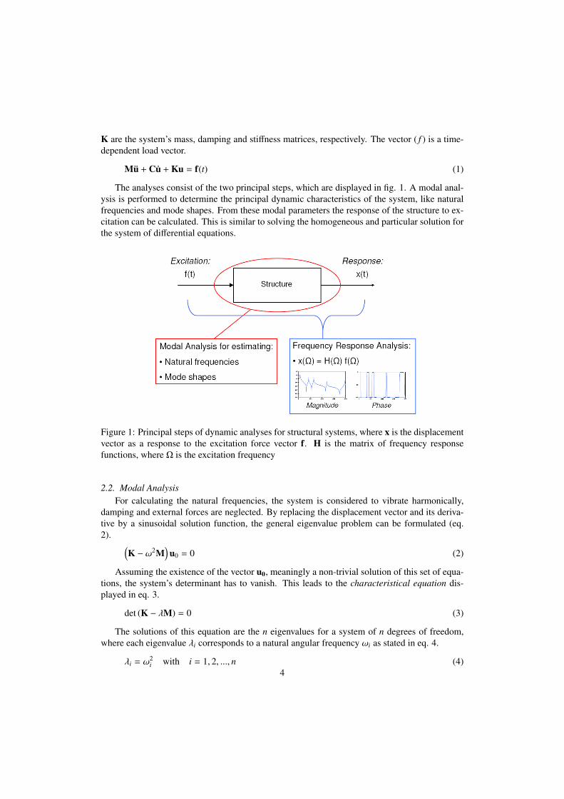
The analyses consist of the two principal steps, which are displayed in fig. 1. A modal anal-ysis is performed to determine the principal dynamic characteristics of the system, like naturalfrequencies and mode shapes. From these modal parameters the response of the structure to ex-citation can be calculated. This is similar to solving the homogeneous and particular solution forthe system of differential equations.

Figure 1: Principal steps of dynamic analyses for structural systems, where x is the displacementvector as a response to the excitation force vector f. H is the matrix of frequency responsefunctions, where Ω is the excitation frequency

2.2. Modal AnalysisFor calculating the natural frequencies, the system is considered to vibrate harmonically,

damping and external forces are neglected. By replacing the displacement vector and its deriva-tive by a sinusoidal solution function, the general eigenvalue problem can be formulated (eq.2). (

K − ω2M)

u0 = 0 (2)

Assuming the existence of the vector u0, meaningly a non-trivial solution of this set of equa-tions, the system’s determinant has to vanish. This leads to the characteristical equation dis-played in eq. 3.

det (K − λM) = 0 (3)

The solutions of this equation are the n eigenvalues for a system of n degrees of freedom,where each eigenvalue λi corresponds to a natural angular frequency ωi as stated in eq. 4.

λi = ω2i with i = 1, 2, ..., n (4)

4

The amplitude vector corresponding to an eigenvalue is the eigenvector or mode shape vectorψi. The combinations of natural frequencies and mode shape vectors describe preferred statesof vibration of the structure [23]. For the numerical estimation of the eigenvalues, several algo-rithms are available, e.g. the Lanczos method [24], which is also available in MSC.Nastran.

2.3. Modal Frequency Response Analysis (Harmonic Analysis)The cornerstone of modal frequency response analyses is the diagonalization of the system’s

matrices by a modal transformation. In a seperation approach the primary variables are replacedby a linear combination of the so-called modal coordinates and the mode shape vectors, as shownin eq. 5, where Ψ is the modal matrix and q is the vector of modal coordinates.

u(t) = ψ1q1(t) + ψ2q2(t) + ... + ψnqn(t) = Ψq(t) (5)

Due to the orthogonality properties of the mode shape vectors, inserting the approach intoeq. 1 and premultiplying the equation by ΨT leads to eq. 6, which are the decoupled equationsof motion for the analyzed system. For diagonalizing the damping matrix by the mode shapesvectors from the modal analysis, a proportional damping approach [23] has to be assumed.

ΨT MΨq(t) +ΨT CΨq(t) +ΨT KΨq(t) = ΨT f(t) (6)

The system now consists of n equations of motion for single degree of freedom oscillators inform of eq. 7, where mi is the modal mass, ci a modal damping coefficient, ki the modal stiffnessand pi a modal force.

miqi(t) + ciqi(t) + kiqi(t) = pi(t) with pi(t) = ψTi f (7)

The equation can be normalized by the modal mass, so that the coefficients are expressed interms of natural angular frequencies ωi and modal damping ratios ζi, as they are defined in eq. 8.This leads to eq. 9.

ω2i = ki/mi and ζi =

12

ci√

kimi(8)

qi(t) + 2ζiωiqi(t) + ω2i qi(t) =

pi(t)mi

(9)

Eq. 9 is an ordinary differential equation of second order that has the solution stated in eq.10 which can be derived by a complex approach where Ω is the excitation frequency. Here,the variable q has already been transformed in the frequency domain which is noted by thecircumflex.

qi(Ω) =1

ω2i −Ω2 + 2 jζiωiΩ

·pi

mi(10)

From here the matrix of frequency response functions (FRFs) can easily be derived, since thefrequency response functions are defined as the displacement response functions multiplied bythe inverse of the excitation force vector (eq. 11).

H(Ω) = u(Ω)f−1(Ω) =

n∑i=1

ψiqi(Ω)f−1(Ω) =

n∑i=1

ψi1

ω2i −Ω2 + 2 jζiωiΩ

·ψT

i

mi(11)

5

For a certain degree of freedom k, the frequency response function due to an excitation forceat the l-th degree of freedom can than be calculated by eq. 12.

Hkl(Ω) =

n∑i=1

ψikψil

mi

(ω2

i −Ω2 + 2 jζiωiΩ) (12)

If the natural frequencies and damping ratios are known, this equation can be evaluated fordiscrete excitation frequencies.

3. Experimental Procedures

3.1. Material and Specimens

The goal is to provide the data which is necessary for performing and validating the damagelocalization approach presented later. Several specimens have been fabricated and have under-gone vibration testing in the undamaged and damaged state [13],[14].

Resin-containing carbon-fiber/epoxy prepregs of T300/914 are used to fabricate the test spec-imens. The material is supplied by Hexcel composites, the physical properties are set out in tab.1. The specimens are processed in a press. The curing cycle of the laminates is 2h at 180C witha warming-up cycle of 0.5h at 135C. The laminates are cut into beams using a diamond wheelcutter, following the ASTM D3039/D3470 standards. The specimens have a thickness of 3mmand consist of 24 plies. The lay-up is chosen as such as the delamination is said to have moreprofound effects on the dynamic characteristics [25].

Table 1: Properties of pre-impregnated carbon/epoxy T300/914 plies

Property Symbol ValueYoung’s modulus in fibre direction E1 122000MPaYoung’s modulus in transverse direction E2 8500MPaShear modulus G12 3570MPaPoisson ratios ν12; ν23; ν31 0.25; 0.3; 0.017Fibre volume ratio 60%Density ρ 1550kg/m3

Number of plies 24Stacking sequence [(0/90/45/ − 45)3]s

The vibration tests are carried out with two steel masses attached at the ends. The aim ofputting these masses at the ends is to enhance the difference in the modal parameters betweenthe undamaged and the damaged test specimens [26].

3.2. Vibration Tests

The experimental equipment used for vibration testing is shown in fig. 2b. The experimentalset-up is that of a free-free beam excited at its center, based on the Oberst beam method [27].This method states that a free-free beam excited at its center shows the same dynamical behavioras that of a half length cantilever beam. The test specimen is placed centered on a B&K forcesensor (type 8200), which is then assembled on a shaker supplied by Prodera, having a maximum

6

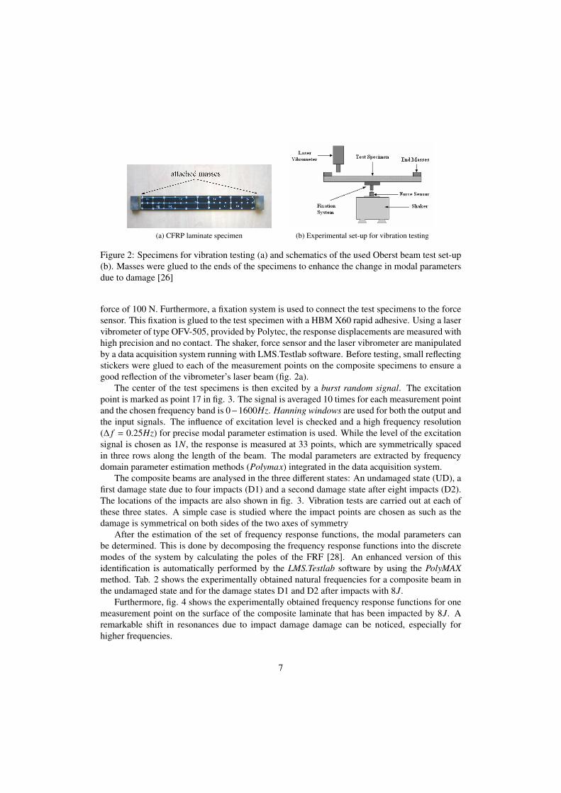
(a) CFRP laminate specimen (b) Experimental set-up for vibration testing

Figure 2: Specimens for vibration testing (a) and schematics of the used Oberst beam test set-up(b). Masses were glued to the ends of the specimens to enhance the change in modal parametersdue to damage [26]

force of 100 N. Furthermore, a fixation system is used to connect the test specimens to the forcesensor. This fixation is glued to the test specimen with a HBM X60 rapid adhesive. Using a laservibrometer of type OFV-505, provided by Polytec, the response displacements are measured withhigh precision and no contact. The shaker, force sensor and the laser vibrometer are manipulatedby a data acquisition system running with LMS.Testlab software. Before testing, small reflectingstickers were glued to each of the measurement points on the composite specimens to ensure agood reflection of the vibrometer’s laser beam (fig. 2a).

The center of the test specimens is then excited by a burst random signal. The excitationpoint is marked as point 17 in fig. 3. The signal is averaged 10 times for each measurement pointand the chosen frequency band is 0−1600Hz. Hanning windows are used for both the output andthe input signals. The influence of excitation level is checked and a high frequency resolution(∆ f = 0.25Hz) for precise modal parameter estimation is used. While the level of the excitationsignal is chosen as 1N, the response is measured at 33 points, which are symmetrically spacedin three rows along the length of the beam. The modal parameters are extracted by frequencydomain parameter estimation methods (Polymax) integrated in the data acquisition system.

The composite beams are analysed in the three different states: An undamaged state (UD), afirst damage state due to four impacts (D1) and a second damage state after eight impacts (D2).The locations of the impacts are also shown in fig. 3. Vibration tests are carried out at each ofthese three states. A simple case is studied where the impact points are chosen as such as thedamage is symmetrical on both sides of the two axes of symmetry

After the estimation of the set of frequency response functions, the modal parameters canbe determined. This is done by decomposing the frequency response functions into the discretemodes of the system by calculating the poles of the FRF [28]. An enhanced version of thisidentification is automatically performed by the LMS.Testlab software by using the PolyMAXmethod. Tab. 2 shows the experimentally obtained natural frequencies for a composite beam inthe undamaged state and for the damage states D1 and D2 after impacts with 8J.

Furthermore, fig. 4 shows the experimentally obtained frequency response functions for onemeasurement point on the surface of the composite laminate that has been impacted by 8J. Aremarkable shift in resonances due to impact damage damage can be noticed, especially forhigher frequencies.

7

Figure 3: Location of impacts and measurement points on composite beams [13]

Table 2: Estimated resonance frequencies for a composite beam before and after impacting (Im-pact energy: 8J / PolyMAX method)[13]

Frequencies [Hz]State 1st bending mode 2nd bending mode 3rd bending mode 4th bending mode

undamaged 35.9 284.2 717.0 1416.84 Impacts 36.4 279.2 687.9 1363.38 Impacts 36.1 270.8 678.7 1236.5

Figure 4: Frequency response functions for point 2 (cp. fig. 3) for a beam impacted with 8J ob-tained by vibration testing. This figure qualitatively highlights the shifts in resonance frequenciesfrom tab. 2

8

4. Optimization Problem Formulation for Damage Localization

For formulating general optimization statements suitable for computation, some general def-initions have to be established. In the beginning, an objective of the optimization has to beidentified as a function of the design variables that are changed in the course of the optimiza-tion. Since the principle objective of the performed optimizations is the matching of a set ofmodal parameters, any kind of matching function (e.g. least square formulations) can be consid-ered. In the present case, due to the nature of the BigDOT optimization algorithm [29], which isbased on exterior point penalty functions, a pseudo objective function formulation is constructedwhere the parameters, which are to be matched, are included as constraints. By the automaticperformance of convergence checks for each of the frequency constraints, the number of consid-ered design responses is practically dynamically adapted in every optimization cycle, dependingon the fulfillment or non-fulfillment of the constraints. In preliminary tests, this formulationalso generally gave more precise results compared to alternative formulations based on finding asearch direction from minimizing the least square of all responses together, for example.

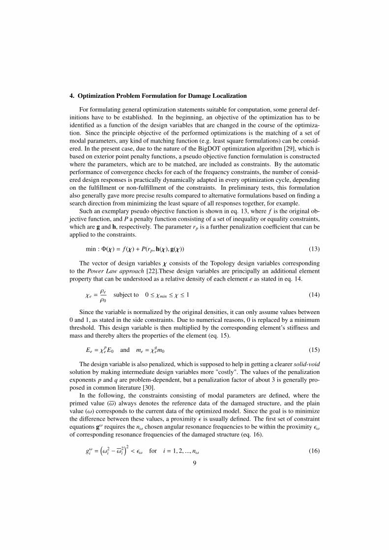
Such an exemplary pseudo objective function is shown in eq. 13, where f is the original ob-jective function, and P a penalty function consisting of a set of inequality or equality constraints,which are g and h, respectively. The parameter rp is a further penalization coefficient that can beapplied to the constraints.

min : Φ(χ) = f (χ) + P(rp,h(χ), g(χ)) (13)

The vector of design variables χ consists of the Topology design variables correspondingto the Power Law approach [22].These design variables are principally an additional elementproperty that can be understood as a relative density of each element e as stated in eq. 14.

χe =ρe

ρ0subject to 0 ≤ χmin ≤ χ ≤ 1 (14)

Since the variable is normalized by the original densities, it can only assume values between0 and 1, as stated in the side constraints. Due to numerical reasons, 0 is replaced by a minimumthreshold. This design variable is then multiplied by the corresponding element’s stiffness andmass and thereby alters the properties of the element (eq. 15).

Ee = χpe E0 and me = χ

qem0 (15)

The design variable is also penalized, which is supposed to help in getting a clearer solid-voidsolution by making intermediate design variables more "costly". The values of the penalizationexponents p and q are problem-dependent, but a penalization factor of about 3 is generally pro-posed in common literature [30].

In the following, the constraints consisting of modal parameters are defined, where theprimed value (ω) always denotes the reference data of the damaged structure, and the plainvalue (ω) corresponds to the current data of the optimized model. Since the goal is to minimizethe difference between these values, a proximity ε is usually defined. The first set of constraintequations gω requires the nω chosen angular resonance frequencies to be within the proximity εωof corresponding resonance frequencies of the damaged structure (eq. 16).

gωi =(ω2

i − ω2i

)2< εω for i = 1, 2, ..., nω (16)

9

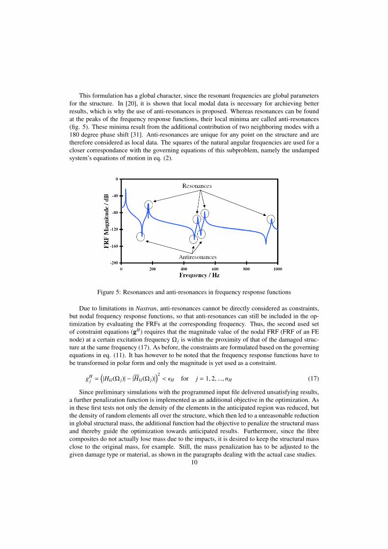
This formulation has a global character, since the resonant frequencies are global parametersfor the structure. In [20], it is shown that local modal data is necessary for archieving betterresults, which is why the use of anti-resonances is proposed. Whereas resonances can be foundat the peaks of the frequency response functions, their local minima are called anti-resonances(fig. 5). These minima result from the additional contribution of two neighboring modes with a180 degree phase shift [31]. Anti-resonances are unique for any point on the structure and aretherefore considered as local data. The squares of the natural angular frequencies are used for acloser correspondance with the governing equations of this subproblem, namely the undampedsystem’s equations of motion in eq. (2).

Figure 5: Resonances and anti-resonances in frequency response functions

Due to limitations in Nastran, anti-resonances cannot be directly considered as constraints,but nodal frequency response functions, so that anti-resonances can still be included in the op-timization by evaluating the FRFs at the corresponding frequency. Thus, the second used setof constraint equations (gH) requires that the magnitude value of the nodal FRF (FRF of an FEnode) at a certain excitation frequency Ω j is within the proximity of that of the damaged struc-ture at the same frequency (17). As before, the constraints are formulated based on the governingequations in eq. (11). It has however to be noted that the frequency response functions have tobe transformed in polar form and only the magnitude is yet used as a constraint.

gHj =

(|Hkl(Ω j)| − |Hkl(Ω j)|

)2< εH for j = 1, 2, ..., nH (17)

Since preliminary simulations with the programmed input file delivered unsatisfying results,a further penalization function is implemented as an additional objective in the optimization. Asin these first tests not only the density of the elements in the anticipated region was reduced, butthe density of random elements all over the structure, which then led to a unreasonable reductionin global structural mass, the additional function had the objective to penalize the structural massand thereby guide the optimization towards anticipated results. Furthermore, since the fibrecomposites do not actually lose mass due to the impacts, it is desired to keep the structural massclose to the original mass, for example. Still, the mass penalization has to be adjusted to thegiven damage type or material, as shown in the paragraphs dealing with the actual case studies.

10

Since the design variables are the elements’ fractional densities, it is more practical to usealso fractional masses for the objective functions, as defined in eq. 18, where m0 is the masswhen the design variables is 1 (solid).

m f ractional =

ne∑ me

m0(18)

Here, ne is the number of elements in the design domain. Due to the constant design volume,this fractional mass is equal to the sum of all fractional densities as shown in eq. 19. Severalobjective functions have been tested, which are laid out in tab. 3.

m f ractional =

ne∑ V0ρe

V0ρ0=

ne∑χe (19)

Table 3: Objective functions for fractional mass penalization

Number Function Derivative(1) L = m f rac(1 − m f rac) L′ = 1 − 2m f rac

(2) L = |1 − m f rac| L′ = −1 for m f rac < 1(3) L = (1 − m f rac)2 L′ = −1 + 2m f rac

In fig. 6 it can then be seen that all functions show a relative minimum at the right end ofthe domain where all fractional densities are 1, but they possess different derivatives, which areimportant for the sensitivity analysis and basically characterize the penalization. The derivativeof function (2) is constant over the whole domain ([0;1]), the derivatives of the other functionsare variable with the fractional mass. Whereas the derivative value of function (1) approachesthe value of the derivative of function (2) close to the right boarder, the derivative of function(3) approaches zero. Therefore, similar results have been obtained using functions (1) and (2)during the simulations. Also, they generally gave better results than function (3).

4.1. Sensitivity Analysis

Since mathematical programming methods usually involve the calculation of gradients of theobjectives for the sensitivity analysis, the derivatives of the constraints with respect to the designvariables are presented in this section. Eq. 20 gives the gradients of the resonance frequenciesthat can be derived from eq. 2 in the frequency domain form as shown in reference [30], whereψie and ψ je are the components of the eigenvectors with respect to the nodal degrees of freedomof the element e.

∂ω2i

∂χe= ψT

ie

(∂Ee

∂χe− ω2

i∂Me

∂χe

)ψ je (20)

The partial derivatives of the frequency response functions have been derived in [32]. Basedon eq. 11, the frequency response function can be written as eq. 21.

H(Ω) = Ψq(Ω)f−1(Ω) (21)

11

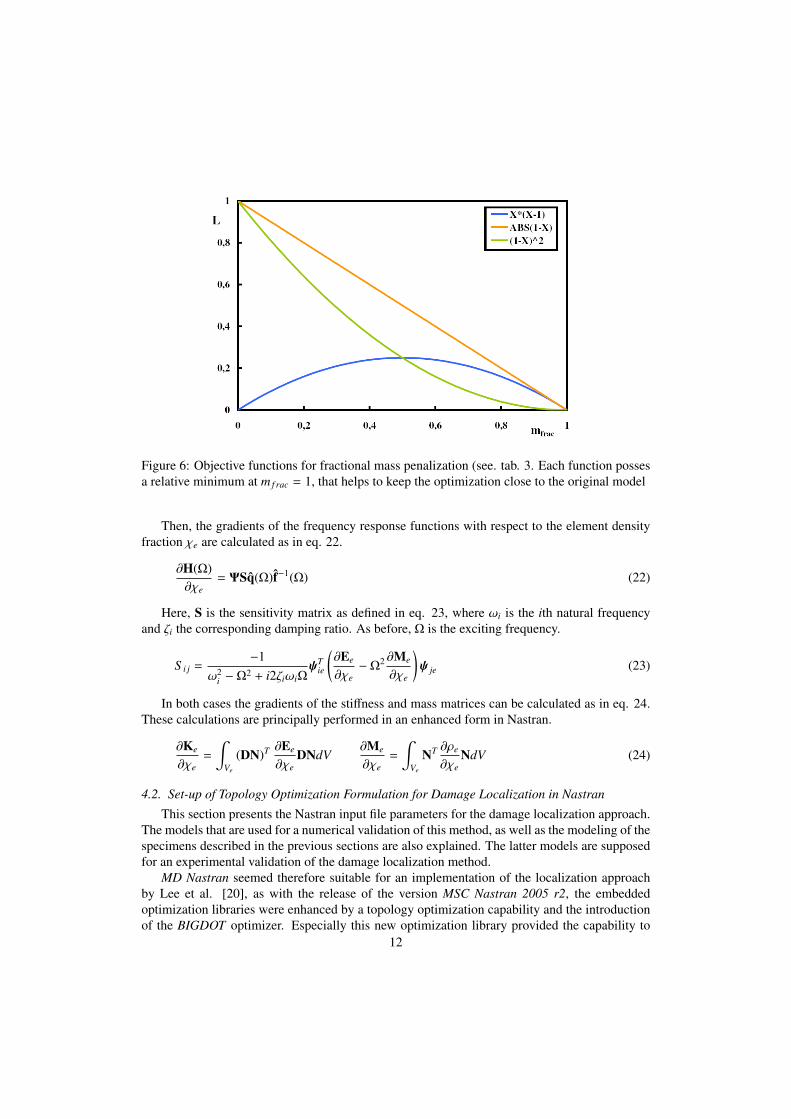
Figure 6: Objective functions for fractional mass penalization (see. tab. 3. Each function possesa relative minimum at m f rac = 1, that helps to keep the optimization close to the original model

Then, the gradients of the frequency response functions with respect to the element densityfraction χe are calculated as in eq. 22.

∂H(Ω)∂χe

= ΨSq(Ω)f−1(Ω) (22)

Here, S is the sensitivity matrix as defined in eq. 23, where ωi is the ith natural frequencyand ζi the corresponding damping ratio. As before, Ω is the exciting frequency.

S i j =−1

ω2i −Ω2 + i2ζiωiΩ

ψTie

(∂Ee

∂χe−Ω2 ∂Me

∂χe

)ψ je (23)

In both cases the gradients of the stiffness and mass matrices can be calculated as in eq. 24.These calculations are principally performed in an enhanced form in Nastran.

∂Ke

∂χe=

∫Ve

(DN)T ∂Ee

∂χeDNdV

∂Me

∂χe=

∫Ve

NT ∂ρe

∂χeNdV (24)

4.2. Set-up of Topology Optimization Formulation for Damage Localization in Nastran

This section presents the Nastran input file parameters for the damage localization approach.The models that are used for a numerical validation of this method, as well as the modeling of thespecimens described in the previous sections are also explained. The latter models are supposedfor an experimental validation of the damage localization method.

MD Nastran seemed therefore suitable for an implementation of the localization approachby Lee et al. [20], as with the release of the version MSC Nastran 2005 r2, the embeddedoptimization libraries were enhanced by a topology optimization capability and the introductionof the BIGDOT optimizer. Especially this new optimization library provided the capability to

12

deliver practical results dealing with the large amount of design variables that are common intopology optimization. Thus, only Nastran was available for an "all at once" implementation ofthe described method combined with low calculation time.

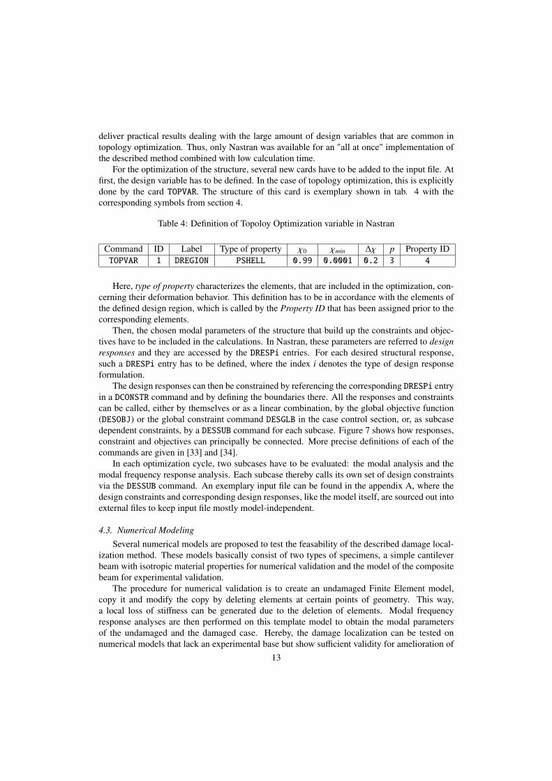
For the optimization of the structure, several new cards have to be added to the input file. Atfirst, the design variable has to be defined. In the case of topology optimization, this is explicitlydone by the card TOPVAR. The structure of this card is exemplary shown in tab. 4 with thecorresponding symbols from section 4.

Table 4: Definition of Topoloy Optimization variable in Nastran

Command ID Label Type of property χ0 χmin ∆χ p Property IDTOPVAR 1 DREGION PSHELL 0.99 0.0001 0.2 3 4

Here, type of property characterizes the elements, that are included in the optimization, con-cerning their deformation behavior. This definition has to be in accordance with the elements ofthe defined design region, which is called by the Property ID that has been assigned prior to thecorresponding elements.

Then, the chosen modal parameters of the structure that build up the constraints and objec-tives have to be included in the calculations. In Nastran, these parameters are referred to designresponses and they are accessed by the DRESPi entries. For each desired structural response,such a DRESPi entry has to be defined, where the index i denotes the type of design responseformulation.

The design responses can then be constrained by referencing the corresponding DRESPi entryin a DCONSTR command and by defining the boundaries there. All the responses and constraintscan be called, either by themselves or as a linear combination, by the global objective function(DESOBJ) or the global constraint command DESGLB in the case control section, or, as subcasedependent constraints, by a DESSUB command for each subcase. Figure 7 shows how responses,constraint and objectives can principally be connected. More precise definitions of each of thecommands are given in [33] and [34].

In each optimization cycle, two subcases have to be evaluated: the modal analysis and themodal frequency response analysis. Each subcase thereby calls its own set of design constraintsvia the DESSUB command. An exemplary input file can be found in the appendix A, where thedesign constraints and corresponding design responses, like the model itself, are sourced out intoexternal files to keep input file mostly model-independent.

4.3. Numerical Modeling

Several numerical models are proposed to test the feasability of the described damage local-ization method. These models basically consist of two types of specimens, a simple cantileverbeam with isotropic material properties for numerical validation and the model of the compositebeam for experimental validation.

The procedure for numerical validation is to create an undamaged Finite Element model,copy it and modify the copy by deleting elements at certain points of geometry. This way,a local loss of stiffness can be generated due to the deletion of elements. Modal frequencyresponse analyses are then performed on this template model to obtain the modal parametersof the undamaged and the damaged case. Hereby, the damage localization can be tested onnumerical models that lack an experimental base but show sufficient validity for amelioration of

13

Figure 7: Construction of objective functions and global or subcase design constraints in Nastraninput files.

the method prior to the performance of experiments. This process has also been performed in thearticle by Lee et al. [20].

A cantilever beam test model with homogeneous isotropic material properties is shown in fig.8a, which was meshed with iso-parametric membrane-bending shell elements. This figure alsoshows the applied constraints and load. On the free end of the beam a nodal frequency-dependentexcitation force with constant amplitude was applied.

(a) Finite element model of a cantilever beamwith applied forces and constraints that has beenused as the initial design for preliminary tests ofthe damage localization method.

(b) Finite element model for analysed compos-ite beams. The point used for comparison of fre-quency response functions is marked.

Figure 8

The experimentally tested beams have also been modeled by shell elements. Due to thesymmetry of the beams and the vibration test setup, it was sufficient to model only a half beamwith the corresponding boundary constraints at the intersection of the the two halves [27]. Forthe nodes at this intersection the displacements in direction of the excitation force were allowed,

14

whereas all other degrees of freedom had to be constrained. Furthermore, the connecting pieceand the end masses that were glued to the specimens for the vibrations tests had to be explicitelymodelled by three-dimensional solid elements. A distributed load with a combined amplitude of1N has been applied to the bottom of the connecting piece to simulate the excitation force of theshaker pot.

Since, at the moment, the topology optimization feature in Nastran is still limited to isotropicmaterials only, the application of the code is also limited to thin quasi-isotropic laminates, forwhich a plane stress state assumption can be made. Mean stiffnesses can then be calculatedbased on the laminate theory [1], reducing whole laminate to a two-dimensional shell. Usingmaterial properties calculated from such a homogenization of the laminate, the composite beamscan be modeled by membrane-bending shell elements as shown in fig. 8b. As mentioned before,damping is not considered in the updating process, since there is no response for damping valuesimplemented in the optmizition module of Nastran. Therefore, a low constant modal dampingvalue of 0,3% has been chosen.

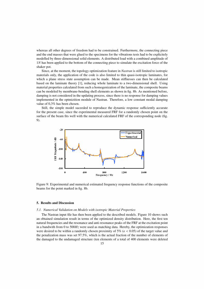
Still, the simple model suceeded to reproduce the dynamic response sufficiently accuratefor the present case, since the experimental measured FRF for a randomly chosen point on thesurface of the beam fits well with the numerical calculated FRF of the corresponding node (fig.9).

Figure 9: Experimental and numerical estimated frequency response functions of the compositebeams for the point marked in fig. 8b.

5. Results and Discussion

5.1. Numerical Validation on Models with isotropic Material PropertiesThe Nastran input file has then been applied to the described models. Figure 10 shows such

an obtained simulation result in terms of the optimized density distribution. Here, the first tennatural frequencies and the resonance and anti-resonance peaks of the FRF at the excitation pointin a bandwith from 0 to 500Hz were used as matching data. Hereby, the optimization responseswere desired to be within a randomly chosen proximity of 5% (ε < 0.05) of the target value andthe penalization mass was set 97.5%, which is the actual fraction of the number of elements ofthe damaged to the undamaged structure (ten elements of a total of 400 elements were deleted

15

for creating the cut out in the damaged template model 10). Although, this test case is based onlyon numerical models, where the location of damage and the loss in mass was known in advance,the approach can be considered as reproducible with physical specimen. Since, in the actual caseof a loss of mass due to impacts in physical specimen, the mass target fraction can be determinedby weighing the undamaged and damaged structure. If no difference in mass can be measured,the mass target has simply to be set almost equal to 100%, as it is done with the later presentedcomposite beam.

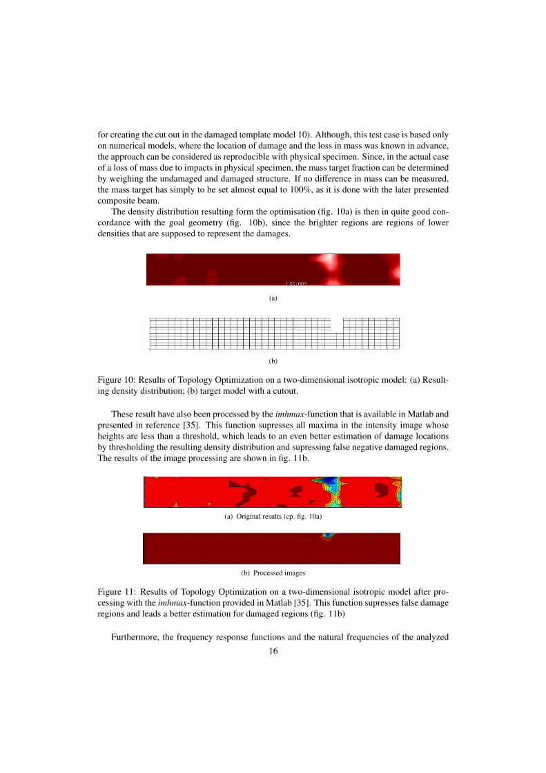
The density distribution resulting form the optimisation (fig. 10a) is then in quite good con-cordance with the goal geometry (fig. 10b), since the brighter regions are regions of lowerdensities that are supposed to represent the damages.

(a)

(b)

Figure 10: Results of Topology Optimization on a two-dimensional isotropic model: (a) Result-ing density distribution; (b) target model with a cutout.

These result have also been processed by the imhmax-function that is available in Matlab andpresented in reference [35]. This function supresses all maxima in the intensity image whoseheights are less than a threshold, which leads to an even better estimation of damage locationsby thresholding the resulting density distribution and supressing false negative damaged regions.The results of the image processing are shown in fig. 11b.

(a) Original results (cp. fig. 10a)

(b) Processed images

Figure 11: Results of Topology Optimization on a two-dimensional isotropic model after pro-cessing with the imhmax-function provided in Matlab [35]. This function supresses false damageregions and leads a better estimation for damaged regions (fig. 11b)

Furthermore, the frequency response functions and the natural frequencies of the analyzed

16

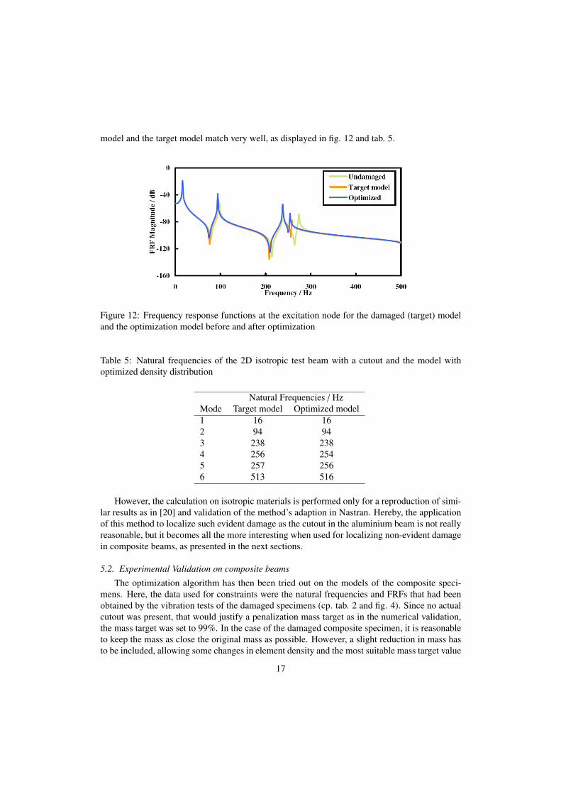
model and the target model match very well, as displayed in fig. 12 and tab. 5.

Figure 12: Frequency response functions at the excitation node for the damaged (target) modeland the optimization model before and after optimization

Table 5: Natural frequencies of the 2D isotropic test beam with a cutout and the model withoptimized density distribution

Natural Frequencies / HzMode Target model Optimized model1 16 162 94 943 238 2384 256 2545 257 2566 513 516

However, the calculation on isotropic materials is performed only for a reproduction of simi-lar results as in [20] and validation of the method’s adaption in Nastran. Hereby, the applicationof this method to localize such evident damage as the cutout in the aluminium beam is not reallyreasonable, but it becomes all the more interesting when used for localizing non-evident damagein composite beams, as presented in the next sections.

5.2. Experimental Validation on composite beams

The optimization algorithm has then been tried out on the models of the composite speci-mens. Here, the data used for constraints were the natural frequencies and FRFs that had beenobtained by the vibration tests of the damaged specimens (cp. tab. 2 and fig. 4). Since no actualcutout was present, that would justify a penalization mass target as in the numerical validation,the mass target was set to 99%. In the case of the damaged composite specimen, it is reasonableto keep the mass as close the original mass as possible. However, a slight reduction in mass hasto be included, allowing some changes in element density and the most suitable mass target value

17

has yet to be determined depending on the problem, which is a limitation of the method at themoment.

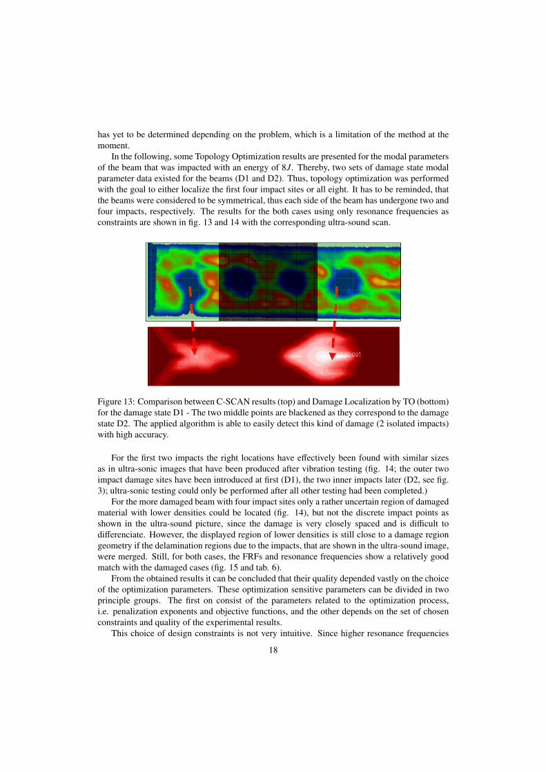
In the following, some Topology Optimization results are presented for the modal parametersof the beam that was impacted with an energy of 8J. Thereby, two sets of damage state modalparameter data existed for the beams (D1 and D2). Thus, topology optimization was performedwith the goal to either localize the first four impact sites or all eight. It has to be reminded, thatthe beams were considered to be symmetrical, thus each side of the beam has undergone two andfour impacts, respectively. The results for the both cases using only resonance frequencies asconstraints are shown in fig. 13 and 14 with the corresponding ultra-sound scan.

Figure 13: Comparison between C-SCAN results (top) and Damage Localization by TO (bottom)for the damage state D1 - The two middle points are blackened as they correspond to the damagestate D2. The applied algorithm is able to easily detect this kind of damage (2 isolated impacts)with high accuracy.

For the first two impacts the right locations have effectively been found with similar sizesas in ultra-sonic images that have been produced after vibration testing (fig. 14; the outer twoimpact damage sites have been introduced at first (D1), the two inner impacts later (D2, see fig.3); ultra-sonic testing could only be performed after all other testing had been completed.)

For the more damaged beam with four impact sites only a rather uncertain region of damagedmaterial with lower densities could be located (fig. 14), but not the discrete impact points asshown in the ultra-sound picture, since the damage is very closely spaced and is difficult todifferenciate. However, the displayed region of lower densities is still close to a damage regiongeometry if the delamination regions due to the impacts, that are shown in the ultra-sound image,were merged. Still, for both cases, the FRFs and resonance frequencies show a relatively goodmatch with the damaged cases (fig. 15 and tab. 6).

From the obtained results it can be concluded that their quality depended vastly on the choiceof the optimization parameters. These optimization sensitive parameters can be divided in twoprinciple groups. The first on consist of the parameters related to the optimization process,i.e. penalization exponents and objective functions, and the other depends on the set of chosenconstraints and quality of the experimental results.

This choice of design constraints is not very intuitive. Since higher resonance frequencies

18

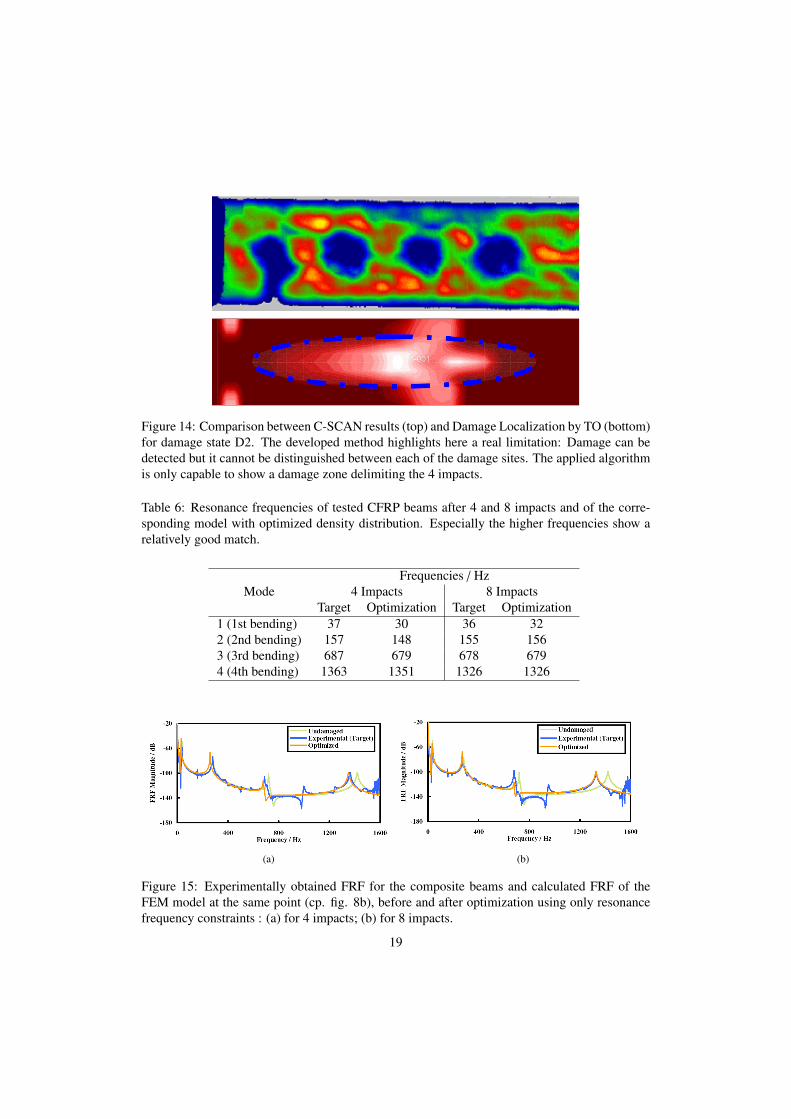
Figure 14: Comparison between C-SCAN results (top) and Damage Localization by TO (bottom)for damage state D2. The developed method highlights here a real limitation: Damage can bedetected but it cannot be distinguished between each of the damage sites. The applied algorithmis only capable to show a damage zone delimiting the 4 impacts.

Table 6: Resonance frequencies of tested CFRP beams after 4 and 8 impacts and of the corre-sponding model with optimized density distribution. Especially the higher frequencies show arelatively good match.

Frequencies / HzMode 4 Impacts 8 Impacts

Target Optimization Target Optimization1 (1st bending) 37 30 36 322 (2nd bending) 157 148 155 1563 (3rd bending) 687 679 678 6794 (4th bending) 1363 1351 1326 1326

(a) (b)

Figure 15: Experimentally obtained FRF for the composite beams and calculated FRF of theFEM model at the same point (cp. fig. 8b), before and after optimization using only resonancefrequency constraints : (a) for 4 impacts; (b) for 8 impacts.

19

show usually a higher shift due to introduced damages, it seems obvious to use modal parametersof a large spectrum. But with higher frequencies the necessary modal identification becomesmore difficult as higher modes are more susceptible to noise and participate less and less in theactual dynamic response.

The presented Topology Optimization approach is also limited to modal parameter shiftsdue to loss in stiffness and mass, but does not take into account damping, which has proven inexperimental results to be more sensitive to damage than stiffness changes ([13],[14],[36]). Inthe current formulation it is not possible to consider changes in damping as constraints in theoptimization, since no direct response for damping is available in Nastran so far.

Considering the used optimization algorithm, the implemented BigDOT optimizer in Nastranis an up-to-date algorithm with high efficiency and reliability. Since it is based on mathemati-cal programming, it shows however common problems like possible wrong local optima and iscertainly subjected to further developments in numerical optimization. Therefore, for a moredetailed validation of the here presented tool, more studies on the optimization parameters andother damage cases are necessary. Still, BigDOT is one of the most capable optimization solu-tions readily available at the moment and it is especially capable of solving topology optimizationproblems [29]. Further studies using different optimisation algorithms (stochastic or evolution-ary methods, etc.) are encouraged, the principal problem in this damage localisation approach ishowever still the inclusion of further design responses that are sensitive to damages in the fibrecomposites.

6. Conclusions

In this paper an enhanced Topology Optimization technique for damage localization is devel-oped based on the works of Lee et al. [20]. In the first part of this paper, the theoretical aspectsof this technique are explained, and in the second part, validations of this technique are carriedout on numerical models and also composite beams.

The presented damage localization approach can also be divided into two sub-problems, theoptimization routine using Topology Optimization and the experimental estimation of modalparameters with the correct numerical modeling.

Concerning the results of the numerical validation, it can be concluded that the feasibility ofapplying the Topology Optimization approach for damage localization is proven also for an im-plementation in Nastran. This provides the opportunity for a broader application of the method,especially to more complex structures, that can be more efficiently analyzed in standard industrialfinite element codes than in self written codes.

In the process of experimental validation, we succeed in localizing seperate damage zones,but the results become less clear and the optimization might get stuck in wrong local optimaregarding the results of C-Scans of the specimens. But it can be assumed, that the poor resultsfor the D2 damage case follow from the simplistic modeling, the lack of constraint data and nottaking into account damping changes, rather than due to a conceptional error in the approach.Still, with a suitable choice of parameters, some good results with correct localization of theimpacts on the composite beams can be archieved.

However, the approach has yet only been validated for one composite laminate beam. In thenear future, this study shall be extended to all the other composite beams tested in reference [14].The approach shall also be applied to localizing damage in standard sandwich specimens withhoneycomb and foam cores, as C-Scan testing is not very capable of detecting damage in com-posite sandwiches. Further prospects of this work could be an optimization using more design

20

responses, like directly addressing the mentioned anti-resonances or mode shapes by referencingthe imaginary part of the FRFs, and to increase the analysed frequency bandwidth to take intoaccount higher modes.

Acknowledgements

The authors gladly thank PhD student Thibault Gouache for his contributions to this articleand to the structural dynamics work group of the ISAE Toulouse.

Appendix

A. Nastran Input File for Damage Localization by Topology Optimization

This Nastran input file can generally be applied to finite element models when the correctmodel geometry and optimization constraints are included and the commented parameters areadjusted.

$--------File Managementsection-----------------------$--------Executive Control Section--------------------SOL 200TIME 20CEND$--------Global Case Control Section------------------TITLE = Damage localizationECHO = NONE$--SOL 200 specific Parameters:MAXLINES = 999999SET 1 = 101 $ Excitation LoadsetSET 2 = 459,254 $ Nodes to be included in CalculationDESOBJ = 201 $ Design Object referencing a Design Response$---------------Subcases------------------------------SUBCASE 1$--Name of Subcase:SUBTITLE = Modal AnalysisANALYSIS = MODESMETHOD = 1 $ Lanczos methodSPC = 2DESSUB = 300 $ Set of design constraints associated with natural frequenciesDRSPAN = 1 $ FRMASS response calculation

SUBCASE 2$--Name of Subcase:SUBTITLE = Frequency ResponseANALYSIS = MFREQ $ Modal frequency response analysisMETHOD = 1FREQUENCY = 1 $ Frequency table for FRF calculationSPC = 2DLOAD = 2LOADSET = 4SDAMPING = 1 $ Damping includedDISP(PHASE) = 2DESSUB = 320 $ Set of Design Constraints FRF Data

$---------------Bulk Data Section---------------------BEGIN BULK$---------------Parameters----------------------------PARAM POST 0PARAM PRTMAXIM YES$--FE Analysis related parameters:PARAM RESVEC YES$--Optmization related parameters:PARAM DESPCH 10$--Frequency table for FRF calculationsFREQ1 1 0. 1. 1600

21

$--Table for modal damping ratiosTABDMP1 1 CRIT

0. 0.003 1600. 0.003 ENDT$--Eigenvalue extraction tableEIGRL 1 20 0$---------------Geometry------------------------------$--Include Model file here (*.bdf)INCLUDE ’modelgeometry.bdf’$---------------BCs-----------------------------------$--referencing BCs in geometry fileSPCADD 2 1$---------------LOADs---------------------------------$--referencing Loads in geometry fileRLOAD1 3 5 1LSEQ 4 5 1DLOAD 2 1. 1. 3$--Frequency dependent load amplitudeTABLED1 1

0. 1. 1600. 1. ENDT$---------------Further Parameters--------------------$--Topoly Optimisation Variable$--(Choice of correct design domain!)TOPVAR 1 PSHELL PSHELL 0.99 .0001 .3 2. 4$--Include optimization constraints file hereINCLUDE ’optimizationconstraints.bdf’$--Objective FunctionDRESP1 101 OBJ FRMASSDRESP2 201 EQART 401

DRESP1 101$--Objective Functions$ 1$DEQATN 401 F1(X)=0.99*X-X**2$ 2DEQATN 401 F1(X)=ABS(0.99-X)$ 3$DEQATN 401 F1(X)=(0.99-X)**2$--Optimisation ParametersDOPTPRM CONV1 .001 DESMAX 50 CONVDV 1e-6 CONVPR 1e-6$--------------End------------------------------------ENDDATA

References

[1] S. W. Tsai, H. T. Hahn, Introduction to Composite Materials, Technomic, Lancaster, Pennsylvania, 1980.[2] M. Y. Kashtalyan, C. Soutis, Mechanisms of internal damage and their effect on the behavior and properties of

cross-ply composite laminates, International Applied Mechanics 38 (6) (2002) 3–22.[3] M. Gude, W. Hufenbach, I. Koch, R. Protz, Fatigue failure criteria and degradation ruls for composites under

multiaxial loadings, Mechanics of Composite Materials 42 (5) (2006) 631–641.[4] V. Li, T. Kanda, Z. Lin, Influence of fibre/matrix interface properties on complementary energy and composite

damage tolerance, Key Engineering Materials 145 (1998) 465.[5] R. M. Gadelrab, The effect of delamination on the natural frequencies of a laminated composite beam, Journal of

Sound and Vibration 197 (3) (1996) 172–181.[6] Y. Yan, L. Cheng, Z. Wu, L. Yam, Development in vibration-based structural damage detection technique, Mechan-

ical Systems and Signal Processing 21 (2007) 2198–2211.[7] S. W. Doebling, C. R. Farrar, M. B. Prime, D. W. Shevitz, Damage identification and health monitoring of structural

and mechanical systems from changes in their vibration characteristics: A literature review, Tech. rep., ResearchReport LA-13070-MS Los Alamos National Laboratory (1996).

[8] Y. Zou, L. Tong, G. P. Steven, Vibration-based model-dependent damage (delamination) identification and healthmonitoring for composite structures - a review, Journal of Sound and Vibration 230 (2) (2000) 357–378.

[9] S. W. Doebling, C. R. Farrar, M. B. Prime, A summary review of vibration-based damage identification methods,Tech. rep., Los Alamos National Laboratory (1998).

[10] H. Sohn, C. Farrar, F. Hemez, D. Shunk, D. Stinemates, B. Nadler, A review of structural health monitoringliterature, Tech. rep., Los Alamos National Laboratory Report LA-13976-MS. (2001).

22

[11] E. Carden, P. Fanning, Vibration based condition monitoring: A review, Structural Health Monitoring 3 (4) (2004)355–377.

[12] B. Schwarz, M. M.H Richardson, Experimental modal analysis, in: CSI Reliability week, Orlando FL, 1999.[13] A. Shahdin, J. Morlier, Y. Gourinat, Correlating low energy impact damage with changes in modal parameters: A

preliminary study on composite beams., Accepted January 09 in Structural Health Monitoring.[14] A. Shahdin, J. Morlier, Y. Gourinat, Significance of low energy impact damage on modal parameters of composite

beams by design of experiments, Accepted in 7th International Conference on Modern Practice in Stress andVibration Analysis, MPSVA 2009.

[15] J. Tracy, G. Pardoen, Effect of delamination on the natural frequencies of composite laminates, Journal of Com-posite Materials 23 (12) (1989) 1200–1215.

[16] R. D. Adams, R. Cawley, The localization of defects in structures from measurements of natural frequencies,Journal of Strain Analysis 14 (1979) 49–57.

[17] M. H. Richardson, M. A. Mannan, Correlating minute structural faults with changes in modal parameters, Proceed-ings of Spie, International Societe of Optical Engineering 1923 (2) (1993) 893–898.

[18] O. Salawu, Detection of structural damage through changes in frequency: a review, Engineering Structures 19 (9)(1996) 718–723.

[19] Z. Zhang, G. Hartwig, Relation of damping and fatigue damage of unidirectional fibre composites, InternationalJournal of Fatigue 24 (2004) 713–738.

[20] J. S. Lee, J. E. Kim, Y. Y. Kim, Damage detection by the topology design formulation using modal parameters,International Journal for Numerical Methods in Engineering 69 (2007) 1480–1498.

[21] M. P. Bendsoe, N. Kikuchi, Generating optimal topologies in structural design using a homogenization method,Computer Methods in Applied Mechanics in Engineering 35 (1992) 1487–1502.

[22] M. Bendsoe, Optimal shape design as a material distribution problem, Structural Optimization 1 (1989) 193–202.[23] D. J. Ewins, Modal Testing: Theory, Practice and Applications, 1984.[24] M. Hörnlund, A. Papazoglu, Analysis and measurments of vehicle door stru dynamic response, Master’s thesis,

Division of Structural Mechanics, LTH, Lund University, Sweden (2005).[25] D. Saravanos, D.A.Hopkins, Effects of delaminations on the damped dynamic characteristics of composites, Journal

of Sound and Vibration 192 (1995) 977–993.[26] K. Vanhoenacker, J. Schoukens, P. Guillaume, S. Vanlanduit, The use of multisine excitations to characterise dam-

age in structures, Mechanical Systems and Signal Processing 18 (2004) 43–57.[27] J. L. Wojtowicki, L. Jaouen, New approach for measurements of damping properties of materials using oberst

beams, Review of Scientific Instruments 75 (8) (2004) 2569–2574.[28] D. L. . Brown, R. J. Allemang, R. Zimmermann, M. Mergeay, Parameter estimation techniques for modal analysis,

Society of Automotive Engineers Paper No. 790221.[29] G. Vanderplaats, Very large scale optimization, Tech. Rep. NASA/CR-2002-211768, Vanderplaats Research and

Development, Inc., Colorado Springs, Colorado (2002).[30] M. P. Bendsoe, O. Sigmund, Topology Optimization - Theory, Methods and Applications, Springer Verlag, 2003.[31] P. Avitabile, Experimental modal analysis - a simpel non-mathematical presentation, Sound and Vibration 35 (1)

(2001) 20–31.[32] Z.-D. Ma, N. Kikuchi, I. Hagiwara, Structural topology and shape optimization for a frequency response problem,

Computational Mechanics 13 (1993) 157–174.[33] MSC.Software Corporation, Santa Ana, CA, USA, MSC Nastran 2007 r1 - Users Guide for Topology Optimization,

r1 Edition (2007).[34] MSC.Software Corporation, Santa Ana, CA, USA, MSC Nastran 2007 Quick Reference Quide (2007).[35] P. Soille, Morphological Image Analysis: Principles and Applications, Springer Verlag, 1999.[36] D. Montalvão, N. Maia, A. Ribeiro, A review of vibration-based structural health monitoring with special emphasis

on composite materials, The Shock and Vibration Digest 38 (4).

23