On the seismic inverse problem: uniqueness, stability and...

On the seismic inverse problem: uniqueness,stability and reconstruction

Elena Beretta (Politecnico di Milano)

ICERM 6 Nov. 2017

E. Beretta (Politecnico di Milano) ICERM 6 Nov. 2017 1 / 49

Collaborators

Francini and Vessella (University of Florence, Italy),

de Hoop, Zhai and Shi (Rice University, USA) ,


Outline

1 Motivation: Reflection Seismology

2 Mathematical model:time harmonic case, linearized elasticity, isotropic medium

3 The inverse problem

4 Some history

5 Regularization: Unknown parameters are piecewise constant on afinite partition of the background domain

6 Parameter identification (given the partition)

7 Quantitative Lipschitz stability estimates

8 Reconstruction algorithm

9 Partition identification

10 Final remarks


Part I

Formulation of the problem


Motivation

Reflection Seismology

Nondestructive testing of materials


Model

Time harmonic elastic wave equation

div(C∇u) + ω2ρu = 0

where C is the elasticity isotropic tensor and ρ the density, ω frequency

Lame system of elasticity (ω = 0)

div(C∇u) = 0


Mathematical formulation

div(C∇u) + ω2ρu = 0 in Ω ⊂ R3

u = ψ on ∂Ω,

∇u := 12

(∇u + (∇u)T

)strain tensor

ψ ∈ H1/2(∂Ω) boundary displacement field,

C elasticity tensor: isotropic, bounded and strongly convex

C = λI3 ⊗ I3 + 2µIsym,

α0 ≤ µ ≤ α−10 , β0 ≤ 2µ+ 3λ ≤ β−1

0 ,

ρ densityγ0 ≤ ρ ≤ γ−1

0


Well-posedness of the direct problem

Let λ01 be the smallest Dirichlet eigenvalue of the operator − div(C0∇) in

Ω, where C0 = β0−3α02 I3 ⊗ I3 + 2α0Isym (so that C ≥ C0). Then, for any

ω2 ∈ (0,γ0λ

01

2]

there exists a unique weak solution u ∈ H1(Ω) ofdiv(C∇u) + ω2ρu = 0 in Ω ⊂ R3

u = ψ on ∂Ω.

Define the Dirichlet to Neumann map ΛC,ρ : H1/2(∂Ω)→ H−1/2(∂Ω)

ΛC,ρψ = (C∇u)ν|∂Ω


Formulation of the inverse problem

Seismic inverse problem

Determine C = (µ, λ) and ρ from knowledge of the Dirichlet-to Neumannmap ΛC,ρ


Key issues

Uniqueness

Stability

Reconstruction


Uniqueness

Static elastic case: ω = 0

Ikehata (1990): linearized version.

Akamatsu, Nakamura and Steinberg (1991) 2D , Nakamura,Uhlmann (1995) 3Dλ, µ ∈ C∞ implies determination of λ, µ and their derivatives on theboundary of a smooth domain.

Nakamura and Uhlmann (2003), Eskin and Ralston (2002) 3DUniqueness of Lame coefficients λ, µ from the DtN map ifλ, µ ∈ C∞(Ω) and µ is close to a constant

Nakamura and Uhlmann, 1993 2D Uniqueness λ, µ ∈ C∞(Ω) andλ, µ are close to a constant

Imanuvilov, Yamamoto, (2013) 2DGlobal result for C 10 Lame coefficients.


Uniqueness

Case ω 6= 0Acoustic time harmonic waves

∇ · (γ∇u) + qω2u = 0

Nachman (1988): Uniqueness of γ ∈ C 2 and q ∈ L∞ with DtoN maps attwo different admissible frequencies.a > 0, c > 0

−∇ · (a∇u) + cu = 0,

Arridge-Lionheart (1998) nonuniquenessHarrach (2012) uniqueness piecewise constant diffusion and absorption


Conditional Stability

Concerning stability: logarithmic (or worse) one is expected, (conductivityinverse problem: Mandache 2001).

Strategy:Look for a-priori assumptions on the unknown parameters

physically relevant

give rise to a better type of stability


Regularization

Small volume conductivity inhomogeneities: Friedman-Vogelius(1989), Vogelius-Fenjia -Moskow (1998), Ammari-B.-Francini(2006).....

Small volume elastic inhomogeneities:Ammari-Kang-Nakamura-Tanuma (2002),B.-Bonnetier-Francini-Mazzucato (2012)

Finite parametrization of conductivities

γ =N∑j=1

γjχDj ,

N⋃j=1

D j = Ω

Alessandrini-Vessella (2005), B.-Francini (2011) (complexcase), Gaburro-Sincich (2015) (anisotropic case)

⇒ Lipschitz stability estimates


Part III

Main results


Main assumptions

C(x) =N∑

m=1

(λmδijδkl + µm(δkiδlj + δkjδli ))χDm(x)

ρ(x) =N∑

m=1

ρmχDm(x)

DjNj=1, disjoint Lipschitz, partition of Ω.


Main goal

1 Parameter estimation (determination of λj , µj , ρj , j = 1, · · · ,N),

2 Interface identification (determination of Dj , j = 1, · · · ,N)


Part IV

Parameter estimation


Main assumptions on the partition Dj1≤j≤N

and on Ω

(H1) Ω, Dj1≤j≤N Lipschitz domains with constants L, r0

(H2) |Ω| ≤ Ar 30

(H3) Dj1≤j≤N is a partition of Ω,

(H4) ∂D1 ∩ ∂Ω := Σ is flat and ∀j ∈ 2, . . . ,N there existsj1, . . . , jM ∈ 1, . . . ,N such that

Dj1 = D1, DjM = Dj ,

andΣk ⊂ ∂Djk−1

∩ ∂Djk ⊂ Ω ,Σk flat , ∀k = 2, . . . ,M


Polyhedral partition


Part V

The main results


Local DN map

Local Dirichlet to Neumann map

H1/2co (Σ) =

φ ∈ H1/2(∂Ω) : supp φ ⊂ Σ ⊂ ∂Ω

H−1/2co (Σ) topological dual of H

1/2co (Σ).

The local Dirichlet to Neumann is

ΛΣC,ρ : ψ ∈ H

1/2co (Σ)→ (C∇u)n|Σ ∈ H

−1/2co (Σ).


Local DN map

Identify ΛΣC,ρ with the bilinear form on H

1/2co (Σ)× H

1/2co (Σ) by

ΛΣC,ρ(ψ, φ) :=< ΛΣ

C,ρψ, φ >=

∫ΩC∇u : ∇v − ω2ρu · v

∀ψ, φ ∈ H1/2co (Σ) and where u is a solution to the BVP with datum ψ

and v is any H1(Ω) function s. t. v = φ on ∂Ω

Denote by

‖T‖? = sup< Tψ, φ > |ψ, φ ∈ H1/2co (Σ), ‖ψ‖

H1/2co (Σ)

= ‖φ‖H

1/2co (Σ)

= 1

for every T ∈ L(

H1/2co (Σ),H

−1/2co (Σ)

).


Main stability result

B., de Hoop, Francini, Vessella, Zhai (2017)

Theorem

Let ω2 ∈ (0,γ0λ

01

2 ]. Then, there exists a positive constant C depending onL,A,N, α0, β0, γ0, λ

01 such that, for any Ck , k = 1, 2 and ρk we have

dΩ((C1, ρ1), (C2, ρ2)) ≤ C‖ΛΣC1,ρ1 − ΛΣ

C2,ρ2‖?.

where

dΩ((C1, ρ1), (C2, ρ2)) = max‖λ1 − λ2‖L∞(Ω), ‖µ1 − µ2‖L∞(Ω), ‖ρ1 − ρ2‖L∞(Ω)

Static case (ω = 0)B. Francini, S. Vessella (2014)Extension to case of C 1,α interfaces B. Francini, Morassi, Rosset,Vessella (2015)


Main ingredients of the proof

Proof: constructive and based on an iterative procedure

QUANTITATIVE AND GLOBAL FORM OF THE INVERSE MAPTHEOREM

SINGULAR SOLUTIONS: Construction of Green’s function withsingularity close to Σ and study of asymptotic behaviour near Σ.

QUANTITATIVE ESTIMATES OF UNIQUE CONTINUATION FORSOLUTIONS OF ELLIPTIC SYSTEMSUnique continuation property: Let v ∈ H1(K ) be a weak solution to

div(C∇v

)+ ω2ρv = 0 in K ,

which vanishes in an open subset K0 ⊂ K with C constant isotropictensor. Then v = 0 in K .


Quantitative inverse function theorem

PROPOSITION - Bacchelli-Vessella 2006.

Let K ⊂ A ⊂ Rd , K compact, A open,

dist(

K,Rd \ A)≥ M1, and K ⊂ BM2(0).

F : A → B

B Banach space.


Quantitative inverse function theorem

1 F is Frechet differentiable;

2 F ′ uniformly continuous, σ1(·) modulus of continuity of F ′ ;

3 F |K is injective;

4 (F |K)−1 : F (K)→ K uniformly continuous , with modulus ofcontinuity σ2(·)

5

minx∈K,|h|=1

∥∥F ′(x)[h]∥∥ B ≥ q0 > 0.

Then‖x1 − x2‖Rd ≤ C‖F (x1)− F (x2)‖B ∀x1, x2 ∈ K,

where C = max 2M1

σ−12 (δ1)

, 2q0 , for δ1 = 1

2 minδ0,M2 with δ0 = σ−11 (q0

2 ).


Reformulation of the problem

L := (λ1, . . . , λN , µ1, . . . , µN , ρ1, . . . , ρN) ∈ R3N ;

CL =N∑j=1

(λj I3 ⊗ I3 + 2µjISym)χDj(x),

‖L‖∞ = maxj=1,...,N

max|λj |, |µj |, |ρj | .


Reformulation of the problem

Let ω2 ∈ (0,γ0λ

01

2 ] and let

F : K ⊂ A ⊂ R3N → B := L(

H1/2co (Σ),H

−1/2co (Σ)

)F (L) = ΛΣ

L

If F satisfies the assumptions of the proposition then

Theorem 1’

‖L1 − L2‖∞ ≤ C‖F (L1)− F (L2)‖? ∀L1, L2 ∈ K

C depends on L,A,N, α0, β0, γ0, λ01 only.


Differentiability of F and Lipschitzcontinuity of F ′

F is Frechet differentiable in A and

< F ′(L)[H]ψ, φ >=

∫ΩH∇uL : ∇vL − hω2uL · vL dx

where H = CH and h = ρH .

The proof is straightforward being a simple consequence of definition of Fand of F ′.


Injectivity of F|K and uniform continuity of(F|K)−1

A first very rough stability estimates for (F|K)−1 can be derived

σ(t) =

| log t|−η for 0 < t < 1

e ,t − 1

e + 1 for t ≥ 1e ,

where η depend on A, L, α0, β0, N only

‖L1 − L2‖∞ ≤ C∗σN(‖F (L1)− F (L2)‖?) , ∀L1, L2 ∈ K

where

σN(·) = σ · · · σ, (N times)

C∗ depends on A, L, α0, β0, γ0,λ01, N only

Proof is based on construction of singular solutions and on estimates ofunique continuation for solutions of elliptic systems


Injectivity of F ′ and lower bound of F ′

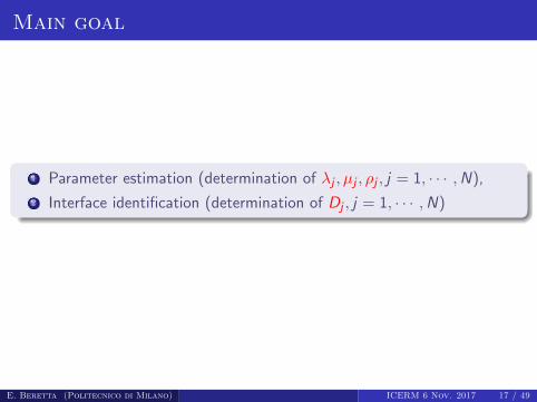
Theorem

Letq0 := min‖F ′(L)[H]‖? | L ∈ K,H ∈ R3N , ‖H‖∞ = 1;

we have(σN1 )−1(1/C?) ≤ q0, (1)

where C? > 1 depends on A, L, α0, β0, γ0, λ01 and N only.

Follows with similar arguments as those used to prove continuity of(F |K)−1


Lipschitz stability in terms of the localNeumann to Dirichlet map

Local Neumann to Dirichlet map

H1/2co (Σ) =

φ ∈ H1/2(∂Ω) : supp φ ⊂ Σ ⊂ ∂Ω

H−1/2(Σ) =

ψ ∈ H−1/2(∂Ω) :< ψ, f >= 0, ∀f ∈ H

1/2co (Σ)

NΣ

C,ρ : ψ ∈ H−1/2(Σ)→ u|Σ ∈ (H−1/2(Σ))∗ ⊂ H1/2(∂Ω)


Lipschitz stability in terms of the LocalNtoD map

Theorem

There exists a positive constant C depending on L,A,N, α0, β0, γ0, λ01

such that, for any Ck , k = 1, 2 and ρk satisfying the stated assumptions

and frequency ω2 ∈ (0,γ0λ

01

2 ]

dΩ((C1, ρ1), (C2, ρ2)) ≤ C‖NΣC1,ρ1 −NΣ

C2,ρ2‖?

where λ01 is the first positive Neumann eigenvalue of the (known) operator

C0 introduced previously.


Lipschitz stability in terms of the localNtoD map

Main Assumption

The elasticity tensor and density are known in a neighborhood of Σ(D1)

Theorem

There exists a positive constant C depending on L,A,N, α0, β0, γ0, λ01

such that, for any Ck , k = 1, 2 and ρk satisfying the stated assumptions

and frequency ω2 ∈ (0,γ0λ

01

2 ]

dΩ((C1, ρ1), (C2, ρ2)) ≤ C‖NΣC1,ρ1 −NΣ

C2,ρ2‖L(L2co(Σ),L2(Σ))

where L2co(Σ) = g ∈ L2(∂Ω) : supp g ⊂ Σ


Reconstruction algorithm

De Hoop, Qiu, Scherzer, 2012

Lipschitz stability estimates ⇒ local convergence of iterativereconstruction methods

m = (C, ρ) and m† = (C†, ρ†) where m† represents the parametercorresponding to the true model.

m = m† in D1 =⇒ NΣm −NΣ

m†Hilbert Schmidt operator

Consider for n sufficiently large the functional

J(m) =1

2

n∑j=1

‖(NΣm −NΣ

m†)gj‖2L2(Σ) ≈

1

2‖NΣ

m −NΣm†‖

2HS

where gj∞1 is an orthonormal basis in L2co(Σ).


Minimization of the Misfit Functional

Constrained Minimization

arg minm∈K

J(m) =1

2

n∑j=1

∫Σ|uj(m)− uj

meas |2 ds

uj weak solution todiv(C∇uj) + ω2ρuj = 0 in Ω ⊂ R3

(C∇uj)ν = g j on ∂Ω


Computation of the gradient

To compute the gradient of the functional J we use Lagrangian approach

L(m, u1, . . . , un, v 1, . . . vn) = J(m) +n∑

i=1

F (v i )− a(m, ui , v i )

where

F (v i ) =

∫Σ

g i · v i

and

a(m, ui , v i ) =

∫ΩC∇ui (x) : ∇v i (x)− ω2ρui (x) · v i (x)

Each v i is Lagrange multiplier associated to a particular constraint i.e. thestate problem with datum g i .


Computation of the gradient of J

From the optimality conditions for L and the chain rule it is easy to seethat

∇mJ(m) = Lm(u1(m), . . . , un(m), v 1(m), . . . vn(m),m)

where u1(m), . . . , un(m) are the state solutions of the direct problem withdatum g 1, . . . , gn and v 1(m), . . . , vn(m) are the adjoint state solutionssatisfying

div(C∇v j) + ω2ρv j = 0 in Ω ⊂ R3

(C∇v j)ν = χΣ(uj − ujmeas) on ∂Ω


Computation of the gradient of J

∇µi J(m) =n∑

j=1

∫Di

∇uj(x) : ∇v j(x)

∇λi J(m) =n∑

j=1

∫Di

∇ · uj(x)∇ · v j(x)

∇ρi J(m) =n∑

j=1

∫Di

uj(x) · v j(x)


Algorithm: Multi-level multifrequencyscheme

Fix a (small) frequency and a coarse model representation

Start from an initial guess and iterate a gradient method

Increase the frequency and fix a finer model representation and againiterate a gradient method starting from the solution of the previousstep as initial guess


Numerical results: Shallow bodies

2.4

2.8

3.2

3.6

2.100

4.000Vp (km/s)

2.4

2.8

3.2

3.6

2.100

4.000Vp (km/s)

1.4

1.6

1.8

2

2.2

1.212

2.309Vs (km/s)

1.4

1.6

1.8

2

2.2

1.228

2.310Vs (km/s)

Figure: On the left: true model of the compressional wavespeedVp and of theshear wavespeed Vs . On the right final reconstruction of Vp,Vs


Numerical results: Deep bodies

2

3

4

1.570

4.500Vp (km/s)

2

3

4

1.570

4.500Vp (km/s)

0.8

1.2

1.6

2

2.4

0.605

2.600Vs (km/s)

0.8

1.2

1.6

2

2.4

0.605

2.600Vs (km/s)

Figure: On the left: true model of Vp and Vs . On the right final reconstructionof Vp,Vs


Part VI

Interface identification


Interface identification

C(x) =N∑

m=1

(λmδijδkl + µm(δkiδlj + δkjδli ))χDm(x)

ρ(x) =N∑

m=1

ρmχDm(x)

”known” parameters λj , µj , ρjunknown domains Dj

Highly nonlinear problem : Identification of a single elastic smoothinterface (log-log stability)Alessandrini-Di Cristo-Morassi-Rosset (2014)


Acoustic time-harmonic wave equation

∆u + ω2qu = 0 in Ω for q =N∑j=1

qjχDj

Theorem

Let

q0 =N∑j=1

q0j χD0

j, q1 =

M∑j=1

q1j χD1

j,

with Dkj regular partitions of tetrahedra, qk

j in a given set of finite,“distinguished” positive values, and ω small enough, there exist ε0 and C0,such that if ‖Λq0 − Λq1‖ ≤ ε0 then

N = M, q0j = q1

j and dH(D0j ,D

1j ) ≤ C0‖Λq0 − Λq1‖

B.- Francini-De Hoop-Vessella (2015)


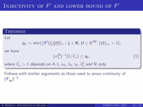
First step towards elasticity case:conductivity equation in 2D

ConsiderF : V ⊂ RdN → L(H−1/2(Σ), (H−1/2(Σ))∗)

where V is the set of vertices of the polygonal partition.Crucial step: Differentiability properties of the map F with respect tovertices and determination of Frechet derivative.Difficulty: Gradients of solutions may blow up at vertices.

γt =N∑j=1

q0j χDt

j

P0j ,i (vertex of D0

j ) ⇒ P0j ,i + tVi ,j (vertex of Dt

j )


First step towards elasticity case:conductivity equation

Let u0 and v0 be solutions todiv (γ0∇u0) = 0 in Ω,

u0 = f on ∂Ω.

div (γ0∇v0) = 0 in Ω,

v0 = g on ∂Ω.

Theorem

d

dt< Λγt f , g >t=0= (k − 1)

∫∂P0

(M0∇ue0 · ∇v e

0 )(Φ~V0 · n0) dσ.

with M0 = τ0 ⊗ τ0 + 1k n0 ⊗ n0 where τ0 and n0 are the tangent and outer

normal directions on ∂P0 and Φ~V0 is the affine function such that

Φ~V0 (P0

j ) = Vj , for j = 1, 2, 3.

B.-Francini-Vessella (2017)

Extends to Voronoi partitions. Extension to arbitrary partitions not known.E. Beretta (Politecnico di Milano) ICERM 6 Nov. 2017 48 / 49

Concluding remarks

1 Prove differentiability of the Dirichlet to Neumann map (Neuman toDirichlet map) with respect to vertices and find the derivative in theelastic case (2D and 3D)

2 Use differentiability properties to prove Lipschitz stability analogousto the acoustic time harmonic case.

3 Compute shape derivative of misfit functional to implement a shapeoptimization based algorithm to recover subsurface rough elasticinterfacesconductivity problem: B.-Micheletti-Perotto-Santacesaria(2017)


Thank you for your attention!


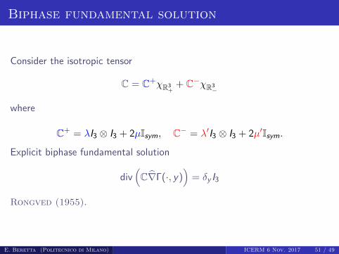
Biphase fundamental solution

Consider the isotropic tensor

C = C+χR3+

+ C−χR3−

where

C+ = λI3 ⊗ I3 + 2µIsym, C− = λ′I3 ⊗ I3 + 2µ′Isym.

Explicit biphase fundamental solution

div(C∇Γ(·, y)

)= δy I3

Rongved (1955).


Construction of the Green’s function

Extend Ω to a new domain Ω0 := Ω ∪ D0 such that ∂Ω0 is ofLipschitz class.

Extend the unknown tensor C and density ρ to Ω0 (still denote by Cthe extension) such that

C|D0A = 2A , for every matrix A

ρ|D0= 1

C = C0χD0(x) +N∑j=1

CjχDj(x)

ρ = ρ0χD0(x) +N∑j=1

ρjχDj(x)


Green’s function

Theorem

Let D = ∪Nj=0∂Dj \ ∪Nk=0Σk . ∀y ∈ Ω0\D, there exists G (·, y), continuousin Ω0 \ y s. t.∫

Ω0

C∇G (·, y) : ∇φ− ω2ρG (·, y) · φ = φ(y), for every φ ∈ C∞0 (Ω0).

G (·, y) = 0 on ∂Ω0.

G (x , y) = G (y , x)T for every x , y ∈ Ω0\D.

‖G (·, y)− Γ(·, y)‖H1(Ω0) ≤ C if dist(y ,D ∪ ∂Ω0)) ≥ r0/C

‖G (·, y)‖H1(Ω0\Br (y)) ≤ Cr−1/2, if dist(y ,D ∪ ∂Ω0)) ≥ r0/C


Estimates of unique continuation

Three Spheres Inequality: Alessandrini- Morassi, (2001)

Estimates for the Cauchy problem: Morassi-Rosset, (2004)

Regularity C∞ at flat interfaces: Chipot-Kinderlehrer-VergaraCaffarelli (1986), Li-Nirenberg, (2003)


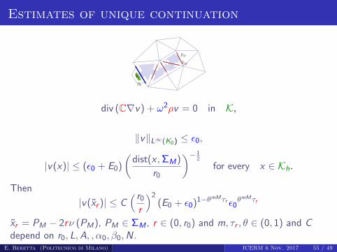
Estimates of unique continuation

div (C∇v) + ω2ρv = 0 in K,

‖v‖L∞(K0) ≤ ε0,

|v(x)| ≤ (ε0 + E0)

(dist(x ,ΣM)

r0

)− 12

for every x ∈ Kh.

Then

|v(xr )| ≤ C( r0

r

)2(E0 + ε0)1−θmMτr ε0

θmMτr

xr = PM − 2rν (PM), PM ∈ ΣM , r ∈ (0, r0) and m, τr , θ ∈ (0, 1) and Cdepend on r0, L,A, , α0, β0,N.


A sketch of the proof of uniform continuityof (F|K)−1

Set C := CL1 and C := CL2 , ρ := ρL1 and ρ := ρL2

ε := ‖ΛΣC,ρ − ΛΣ

C,ρ‖?

Consider the Green’s functions in Ω0 = Ω ∪ D0 corresponding to (C, ρ)and (C, ρ) for y , z ∈ K0 fixed. Then

∫Ω0

(C− C)∇G (·, y) : ∇G (·, z)− ω2(ρ− ρ)G (x , y) · G (x , z) =

< (ΛC,ρ − ΛC,ρ)G (·, z),G (·, y) >

Hence, since dist(K0, ∂D0) ≥ r0/C ,∣∣∣∣∫Ω0

(C− C)∇G (·, y) : ∇G (·, z)− ω2(ρ− ρ)G (x , y) · G (x , z)

∣∣∣∣ ≤ Cε


Sketch of the proof

Define, for y , z ∈ K0

S0(y , z) :=

∫Ω0\D0

(C− C)∇G (·, y) : ∇G (·, z)−ω2(ρ− ρ)G (x , y) · G (x , z),

S0(·, z),S0(y , ·) ∈ H1loc(D0) ∀y , z ∈ D0

div(C∇yS(·,q)0 (·, z)) + ω2ρS(·,q)

0 (·, z)) = 0 in D0,

div(C∇zS(p,·)0 (y , ·)) + ω2ρS(p,·)

0 (y , ·)) = 0 in D0.

|S0(y , z)| ≤ Cε ∀y , z ∈ K0 × K0,

and|S0(y , z)| ≤ C (dist(y ,Σ)dist(z ,Σ))−1/2 , y , z ∈ D0,


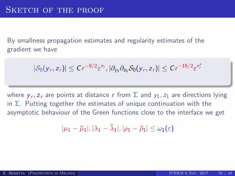
Sketch of the proof

By smallness propagation estimates and regularity estimates of thegradient we have

|S0(y r , z r )| ≤ C r−9/2ετr , |∂y1∂z1S0(y r , z r )| ≤ C r−15/2ετ′r

where y r , z r are points at distance r from Σ and y1, z1 are directions lyingin Σ. Putting together the estimates of unique continuation with theasymptotic behaviour of the Green functions close to the interface we get

|µ1 − µ1|, |λ1 − λ1|, |ρ1 − ρ1| ≤ ω1(ε)


Sketch of the proof

Consider

S1(y , z) :=

∫Ω0\D0∪D1

(C−C)∇G (·, y) : ∇G (·, z)−ω2(ρ−ρ)G (x , y)·G (x , z),

Then, for y , z ∈ K0

|S1(y , z)| ≤ C (ε+ ω1(ε)),

|S1(y , z)| ≤ C (dist(y ,Σ)dist(z ,Σ))−1/2 , y , z ∈ D0 ∪ D1,

So, similarly, using the properties of S1 we can show

|µ2 − µ2|, |λ2 − λ2|, |ρ2 − ρ2| ≤ ω2(ε)

and iterating the argument we get

|µk+1 − µk+1|, |λk+1 − λk+1|, |ρk+1 − ρk+1| ≤ ωk+1(ε)

for all k = 0, . . . ,ME. Beretta (Politecnico di Milano) ICERM 6 Nov. 2017 59 / 49

On the seismic inverse problem: uniqueness, stability and...

Documents

Transcript of On the seismic inverse problem: uniqueness, stability and...