On the Alexander polynomial of lens space knot

Motoo Tange

Institute of Mathematics, University of Tsukuba Ibaraki 305-8571, Japan

e-mail: tange@math.tsukuba.ac.jp

Abstract

Ozsvath and Szabo discovered the coefficients constraints of the Alexander poly-nomial of lens space knot. All the coefficients are either ±1 or 0 and the non-zero coef-ficients are alternating. We here show that the non-zero coefficients give a traversablecurve in a plane R2. This determines the second top coefficient ag−1 easily, and cansee more constraints of coefficients of a lens space knot. In particular, we determinesthe third and fourth non-zero coefficients for lens space knot with at least 4 non-zeroAlexander coefficients. 1 2

1 Introduction.

1.1 Alexander polynomial of lens space knot.

Let Yr(K) denote a r-surgery along K of a homology sphere Y . We call the rationalnumber r slope of the Dehn surgery. L(p, q) is defined to be −p/q-surgery of theunknot in S3. A knot K ⊂ Y is called a lens space knot if an integral Dehn surgeryof K is a lens space. Here we only consider the integer Dehn surgery. Berge in [1]defined doubly primitive knot, which is a class of lens space knots in S3. Conjecturely,doubly primitive knots are all lens space knots in S3. We will define doubly primitiveknot in a homology sphere.

The lens space knot has interesting features as follows. Suppose that K is a lensspace knot in an L-space homology sphere or a doubly primitive knot in a homologysphere. Those lens space knots are fibered knots, which this is proven by Ni [18] andOzsvath-Szabo [13]. Thus the genus g coincides with the degree of the Alexanderpolynomial of the knot K. The coefficients of Alexander polynomials of those lensspace knots are studied by Ozsvath and Szabo [13] and Ichihara-Saito-Teragaito [11].The Alexander polynomials of lens space knot has been also studied in [8], [13], and[15].

Throughout this paper, we deal with the symmetrized Alexander polynomial.

Theorem 1.1 (Ozsvath-Szabo [13], Ichihara-Saito-Teragaito [11]). Suppose that K isan L-space knot in S3, or a doubly primitive knot in a homology sphere Y . Then theAlexander polynomial of K is of form

∆K(t) = (−1)r +r∑

j=1

(−1)j−1(tnj + t−nj ), (1)

1Keyword: lens surgery, Alexander polynomial, doubly primitive knot2MSC: 57M25,57M27

1

for some decreasing sequence of positive integers d = n1 > n2 > · · · > nr > 0.

This theorem holds even if K is a lens space knot in an L-space homology sphere.Theorem 1.1 says that any Alexander polynomial of lens space knot satisfies the fol-lowing: {

The absolute values of coefficients are ≤ 1. (Flat)

The non-zero coefficients alternate in sign. (Alternating)(2)

In particular, the top coefficient of ∆K(t) is 1. The Alexander polynomial of (r, s)-

torus knot T (r, s), which is computed by ∆T (r,s) = t−(r−1)(s−1)

2(trs−1)(t−1)(tr−1)(ts−1) , is typical

example satisfying (2), because the (rs± 1)-surgery of T (r, s) is a lens space. We callthis polynomial a torus knot polynomial. In general, we call the Alexander polynomialof a lens space knot lens surgery polynomial.

We call the sequence (d = n1, · · · , nr) half non-zero sequence (or exponents) andthe decreasing sequence (d = n1, n2, · · · , n2r, n2r+1 = −d) (full) non-zero sequence(or exponents). From the symmetry of the Alexander polynomial n2r+2−i = −ni

holds. We denote the non-zero sequence (or the half non-zero sequence) of a lensspace knot or a doubly primitive knot K by NS(K) or NSh(K) respectively. Forexample, NSh(31) = (1, 0) and

NS(Pr(−2, 3, 7)) = (n1, n2, n3, n4, n5, n6, n7, n8, n9) = (5, 4, 2, 1, 0,−1,−2,−4,−5),(3)

where Pr(−2, 3, 7) is the (−2, 3, 7)-pretzel knot.In this paper we reveal a connection of the non-zero coefficients of the Alexander

polynomial of a lens space knot. This connectivity gives some constraints about thenon-zero sequence or lens surgery knot.

1.2 The genus and lens space surgery

Suppose that the p-surgery Yp(K) of an L-space homology sphere Y is an L-space.Then the following inequality holds:

2g(K) ≤ p+ 1. (4)

In the lens surgery case on Y = S3, actually the inequality can be made sharper as in[4]. Furthermore, there exist lens surgeries satisfying the equality when Y = Σ(2, 3, 5)as in [16].

Here we define Dehn surgery realization.

Definition 1.1. Let K be a lens space knot with Yp(K) = L(p, q) for a homologysphere Y . If there exists a knot K ′ in a homology sphere Y ′ such that Y ′

p(K′) = L(p, q)

and these lens surgeries give the same surgery parameter, then we say that the surgeryYp(K) = L(p, q) can be realized by a lens surgery of K ′.

The surgery parameter (p, k) will be defined in Section 2.1. The parameter k meansthe homology class of the dual knot of lens space surgery.

The nice realization of lens space surgery is the set of doubly primitive knots, whichis defined in [1]. In fact, it is proven in [5] that any lens surgery on S3 can be realizedby a doubly primitive knot in S3. In general, any lens surgery which is an integralDehn surgery of a homology sphere can be realized by a doubly primitive knot in ahomology sphere. We post the following genus bounding conjecture.

Conjecture 1.1. Let Yp(K) be a lens surgery on an L-space homology sphereY . Then,this surgery can be realized by a lens surgery of K ′ of an L-space homology sphere Y ′

with2g(K ′) ≤ p.

2

Furthermore, this realization can assume that K ′ is a doubly primitive knot.

In [17] the author showed some lens surgeries of the Poincare homology spherewith the usual orientation have 2g(K) = p.

Definition 1.2. Let K be a knot in an L-space homology sphere Y . We call lenssurgery Yp(K) = L(p, q) with 2g(K) ≤ p an admissible lens surgery. Such a knot Kis called an admissible lens space knot.

Throughout this paper, we only treat any admissible lens surgeries on an L-spacehomology sphere or doubly primitive knots in homology spheres. The Seifert genusg(K) of those knots coincides with the degree d of the Alexander polynomial. Ras-mussen proved the following:

Theorem 1.2 (Rasmussen [14]). Let K ⊂ Z be a knot in an L-space, and supposethat some integral surgery on K yields a homology sphere Y . If 2g(K) < p + 1, thenY is an L-space, while if 2g(K) > p+ 1, then Y is not an L-space.

Thus, if p is a lens surgery slope of a doubly primitive knot K in a non-L-spacehomology sphere, then 2g(K) ≥ p+ 1 holds.

1.3 Results

LetK be a lens surgery knot with a parameter (p, k). We set the Alexander coefficientsA = {a−d, a−d+1, · · · , ad} on Z2 along the line j = j0 ∈ Z. On the other vertical lineswe also set A with the shift by k or |k2|. Theorem 2.3 says the non-zero coefficients areweakly-increasingly (or decreasingly) traversable in some ways. We call the traversablecurve non-zero curve. This curve is connected and simple.

Results in this section is obtained by using a connectivity of the non-zero curve inthe plane R2 and the property (2).

We mainly deal with the following types of non-trivial lens space knots:

(A) An admissible lens space knot in an L-space homology sphere Y .

(B) A doubly primitive knot in a homology sphere Y .

For example, all the lens space knots in S3 are contained in the knots of type (A).Furthermore, if a lens space is an integral surgery of a homology 3-sphere, which isequivalent to the fact that −q is a quadratic residue in Z/pZ, then L(p, q) can berealized by a knot K of a homology sphere Y with n2(K) = d − 1, where d is theAlexander degree of K.

In the several main theorems the same assertion will be proven for both types (A)and (B) separately, however both types have a traversable property (Theorem 2.3) incommon and for the proofs we use actually the same method.

For example, we can determine the second term as an application of the non-zerocurve. This result was also proven independently in [10] and [7].

Theorem 1.3. Let K ⊂ Y be a non-trivial knot of (A) or (B), then we have

n2 = d− 1. (5)

In particular, any non-trivial lens space knot in S3 satisfies n2 = d− 1.

This property (5) gives an interesting strict constraint. For example, if ∆K(t) isof form f(tm) (e.g., (m, 1)-cable knot of any knot), then m must be 1. Hence, the(m, 1)-cable of any knot for m > 1 is not a lens space knot, which this was alreadyproven in [2].

In the following, we will prove a characterization of lens space knots with (2, n)-torus knot polynomial.

3

Theorem 1.4. Let K ⊂ Y be a non-trivial knot of (A) or (B) with surgery parameter(p, k, k2) and k ≤ |k2|. Then the following conditions are equivalent:

1. ∆K(t) = ∆T (2,2d+1)(t)

2. The lens surgery parameter of Yp(K) = L(p, q) is (p, 2, 2d+ 1).

3. The lens surgery can be realized by the surgery of (2, 2d+ 1)-torus knot

4. |k2| = 2g(K) or |k2| = 2g + 1.

This theorem says that if a doubly primitive knot K in a homology sphere Ysatisfies ∆K(t) = ∆T (2,2d+1)(t), then K is isotopic to T (2, 2d + 1). In particular Yhave to be homeomorphic to S3. Furthermore, we have the following:

Corollary 1.1. For any non-L-space homology sphere Y there exists no doubly prim-itive knot K ⊂ Y with ∆K(t) = ∆T (2,2d+1)(t).

Is this statement true, in general?

Question 1.1. Let K ⊂ Y be a doubly primitive knot in a homology sphere. If∆K(t) = ∆T (r,s)(t), then K is isotopic to T (r, s)?

We give a negative answer for this question by computing the Alexander polynomialof a doubly primitive knot.

Let K be a knot whose Alexander polynomial satisfies with (2). For the non-zerosequence {ni} of the polynomial we define the following index:

α(K) = max{n1 − n2j+1|n2i−1 − n2i = 1, 1 ≤ ∀i ≤ j ≤ r − 1},

where 2r − 1 is the number of the full non-zero sequence. The index α satisfies2 ≤ α(K) ≤ 2d. The condition of the polynomial satisfying the equality α(K) = 2d isequivalent to ∆K(t) = ∆T (2,2d+1). This index α(K) means the length of the maximalregion which contains the top term and coefficients 1,−1 are adjacent.

The non-zero sequence with α(K) = α0 satisfies with

(n1, n2, · · · , n2s−3, n2s−2, n2s−1, · · · ) = (d1, d1 − 1, · · · , ds−1, ds−1 − 1, ds, · · · ),

where d1 − ds = α0. We call the region {i ∈ Z|n2s+1 ≤ i ≤ n1} adjacent region.In this paper we use notations (d1, d2, · · · , ds) for sequence of +1 coefficients in

the adjacent region. It is called the adjacent sequence and denoted by AS(K) anddi−1 > di + 1 for any i ≤ s. Hence, s is the number of +1 in the adjacent region. Forexample, the α(Pr(−2, 3, 7)) = 7, from non-zero sequence (3) and s = 4.

We give the following lower estimate of the index α:

Theorem 1.5. Let K be a lens surgery parameter with (p, k). Then we have

α+ 1 ≥ max{|k2|, k}. (6)

Furthermore, if d1−ds1+1 = |k2| or k holds for some integer s1, then the coefficientof tds1−1 is zero.

If the Alexander polynomial ∆K can be expanded as follows

∆K(t) = td1 − td1−1 + td2 − td2−1 + · · ·+ tdγ−1 − tdγ−1−1 + tdγ − · · · ,

then d1 − dγ + 1 ≥ max{|k2|, k}.From the inequality, we classify lens space knots with α(K) = 2.

Corollary 1.2. Let K be an admissible lens space knot. If α(K) = 2, then the surgerycan be realized by the trefoil knot.

4

Proof. The inequality implies max{k, |k2|} ≤ 3. The surgery parameters with thiscondition are (5, 2), (7, 2), (8, 3) or (10, 3). The parameters (5, 2) and (7, 2) can berealized by the trefoil. The non-zero sequence of the parameters (8, 3) and (10, 3) are(4, 3, 1, 0) and (6, 5, 3, 2, 0) respectively. These sequeces do not satisfy α = 2.

Let AS = (d1, d2, · · · , ds) be an adjacent sequence. We will prove the followingrelationship between the adjacent sequence and the surgery parameter.

Proposition 1.1. Let (p, k) and (d1, · · · , ds) be a surgery parameter of (A) or (B)and the adjacent sequence respectively. Then there exist integers 1 ≤ s1, s2 ≤ s suchthat

ds1 =

{d1 − k

d1 − k + 1and ds2 =

{d1 − |k2|d1 − |k2|+ 1.

The connectivity of the non-zero curve gives a further determination of non-zerocoefficients.

Proposition 1.2. If ds1 = d1 − k + 1 or d1 − |k2| + 1, then α(K) = d1 − ds1 holds.Furthermore one of the following cases holds:

(a) The case of n2s−1 − n2s > 3. Then we have n3 = n2 − 1.

(b) The case of n2s−1 − n2s = 3. Then we have n3 < n2 − 1.

(c) The case of n2s−1 − n2s = 2.

If n2s−1 − n2s = 2 and n2 − n3 = 1, then n2s − n2s+1 = 1 holds.

We immediately get the two corollaries:

Corollary 1.3. Suppose that the surgery parameters (p, k, |k2|) of type (A) or (B)satisfies |k2| = k + 1. Then, α(K) = k holds.

The equality holds when K = T (u, u + 1) where we have u ≥ 2. In this case, wehave k = u and k2 = u+ 1. The expansion of ∆T (u,u+1)(t) is as follows:

∆T (u,u+1)(t) = td − td−1 + td−u − td−u−2 + · · · ,

where d = u(u−1)2 . The non-zero sequence is AS(T (u, u+1)) = (d, d−u) and α(T (u, u+

1)) = u.Theorem 1.3 and 1.5 were proven by the author before in [16], although, here we

reprove by using the global coefficients of Alexander polynomials.

Corollary 1.4. The number r of non-zero exponents of ∆K(t) is bounded as follows:

max{k, |k2|} ≤ 2r + 1.

By using the following results, we determine the third and fourth non-zero coeffi-cients of any lens space knot.

Theorem 1.6. Let (p, k) be a lens surgery knot of type (A) or (B) with at least 4non-zero coefficients of the Alexander polynomial. Then, the third coefficient n3 andfourth coefficient n4 are one of the following.

(n1, n2, n3, n4) = (d, d− 1, d2, d2 − 1), (d, d− 1, d2, d2 − 2), or (d, d− 1, d2, d2 − 3),

where d > d2 + 1. If (p, k) be a lens surgery knot of type (A), then (n1, n2, n3.n4) =(d, d− 1, d2, d2 − 3) does not occur.

5

In particular, the Alexander polynomial of lens space knot K in S3 can be expandedthe following:

∆K(t) = td − td−1 + td2 − td2−1 + · · ·

or∆K(t) = td − td−1 + td2 − td2−2 + · · · .

In Section 3.2, we give all lens surgery with 2g − 4 ≤ |k2| ≤ 2g − 1, in Section 3.3,we give lens surgery g ≤ 5 or with 7 non-zero coefficients

Theorem 1.7. Let (p, k, k2) be a lens space knot of type (A) with 2g(K)− 4 ≤ |k2| ≤2g(K)− 1. Then K can be realized by the following knots:

T (4, 3), or Pr(−2, 3, 7)

These lens surgeries just corresponds to the ones with the half non-zero sequence

(d, d− 1, d− 3, d− 4, · · · , 2, 1, 0).

Theorem 1.8. Let K be a lens space knot with g(K) ≤ 5 of type (A). Then K canbe realized by one of the following:

T (2, 3), T (2, 5), T (2, 7), T (3, 4), T (2, 9), T (3, 5), T (2, 11), or Pr(−2, 3, 7)

The lens surgery of type (B) has g ≥ 6.

Theorem 1.9. Let K be a lens space knot with at most 7 non-zero coefficients of type(A) or (B). Then K can be realized by one of the following:

T (2, 3), T (2, 5), T (4, 3), T (2, 7), T (3, 5), T (4, 5)

Acknowledgements

The author would like express the gratitude for Masaaki Ue, who was my supervisor,and would thank for T. Kadokami’s organizing seminars (was taken place in 2006 and2007) and useful communication there with N. Maruyama and T .Sakai as well. Theauthor was supported by the Grant-in-Aid for JSPS Fellows for Young Scientists(17-1604) and JSPS KAKENHI Grant Number 24840006, and 26800031.

2 Preliminaries

In this section we give several basics of lens space surgery. To prove the main theoremswe define the non-zero curve in the plane and prove that this curve is traversable in anon-zero region, which is called a traversable theorem.

2.1 Lens surgery parameter and Alexander polynomial

Here we review some definitions, notations and formulae used in this paper. Let Ybe a homology sphere. Suppose that the p-surgery of K ⊂ Y yields lens space L(p, q)i.e., Yp(K) = L(p, q). The dual knot K, which is the surgery core of the Dehn surgery,

gives a homology class [K] ∈ H1(L(p, q)). The orientation of K is arbitrarily put. Theclass can be represented as an integer k as follows: [K] = k[C], where C is the coreof genus one Heegaard splitting of L(p, q). The integer k is a multiplicative generatorin (Z/pZ)×. The choice of the core of genus one Heegaard splitting of L(p, q) gives

6

an ambiguity k → k−1 mod p. The change of oriention gives ambiguity k → −k. Wechange the integer k → −k, k−1,−k−1 mod p, if necessary, to get k2 = −q mod p and0 < k < p

2 .We define the integer k2 satisfying kk2 = 1 mod p and −p

2 < k2 < p2 .

Definition 2.1. We call the pair (p, k, |k2|) (lens) surgery parameter of Yp(K) =L(p, q). We omit the third parameter |k2| in some cases. In the case where (p, k, |k2|)give an admissible lens surgery, we call it an admissible parameter.

Theorem 2.1 ([15],[8]). Let Y be a homology sphere and K a lens space knot oftype (A) with surgery parameter (p, k). Then, for an integer l with kl = 1 mod p andgcd(k, l) = 1, we have

∆K(t) ≡ ∆T (k,l)(t) mod tp − 1.

Furthermore, if the surgery is an admissible lens surgery, then ∆K(t) is the smallestrepresentative of ∆T (k,l) in Z[t±1]/(tp − 1).

For a Laurent polynomial f(t) =∑

i βiti ∈ Q[t±1], the smallest representative of

f(t) in mod tp − 1 means

f(t) =

{∑|i|< p

2αit

i p ≡ 1 mod 2∑|i|< p

2αit

i +α p

2

2 (tp2 + t−

p2 ) p ≡ 0 mod 2

,

where αi =∑

j≡i mod p βj . The polynomial f(t) is equivalent to f(t) in Q[t±1]/(tp−1).

Hence, the last statement is equivalent to ∆K(t) = ∆T (k,l)(t).

2.2 The coefficient formula of Alexander polynomial for ad-missible lens surgery.

Here we give the coefficient formula of the Alexander polynomials of admissible lenssurgery knots. This formula has been proven in [15], and we will reprove it as a formulawith a bit different form.

We put e = sgn(k2), c =(k+1−p)(k−1)

2 , m = kk2−1p , and

Iα =

{{1, 2, · · · , α} α > 0

{α+ 1, α+ 2, · · · ,−1, 0} α < 0

The bracket [·]p stands for the least absolute remainder with respect to p. Nemely,the remainder satisfies −p

2 < [y]p ≤ p2 for integer y. In [15] the coefficient ai of the

symmetrized Alexander polynomial ∆K(t) is computed as follows:

Proposition 2.1 ([15]). Let K be a lens space knot of type (A). Suppose that Yp(K) =L(p, q) and 2g(K) < p. Then we have

ai(K) = −m+ e ·#{j ∈ Ik|[−p2(j + ki+ c)]p ∈ Ik2}. (7)

If 2g(K) = p, then

ai(K) =

{−m+ e ·#{j ∈ Ik|[−p2(j + ki+ c)]p ∈ Ik2} |i| < p

2

1 i = ±p2

.

From the upper bound of g(K) by Greene [4] in the case of Y = S3, for the formulaof ai we use (7). Here we prove this proposition. Essentially, this equality (7) wasproven in [15]

7

Proof. We set the right hand side of (7) as αi(K). Then

tlc+1(tk−1)(tl−1)∑

0≤i<p

αiti ≡

∑0≤i<p

(αi−k−l−lc−1−αi−k−lc−1−αi−l−lc−1+αi−lc−1)ti mod tp−1.

(8)Since we have

αi−l − αi = eEk2(−p2(ki+ c))− eEk2

(−p2(k(i+ 1) + c)),

αi−k−l−lc−1 − αi−k−lc−1 − αi−l−lc−1 + αi−lc−1

= eEk2(k2(i− 1)− 1)− eEk2

(k2(i− 1))− eEk2(k2i− 1) + eEk2

(k2i)

=

1 i = k + 2, k

−2 i = k + 1

0 otherwise.

Thus, (8) is tk(t− 1)2. Thus we have

tlc+1(tk − 1)(tl − 1)∆K(t) ≡ tk(tkl − 1)(t− 1) mod tp − 1

Thus, we have

∆K(t) ≡ t−lc−1+k (tkl − 1)(t− 1)

(tk − 1)(tl − 1)(9)

in Q[t±1]/∑p−1

i=0 ti. Here lc+ 1− k = 12 (k − 1)(l − 1) mod p holds. In fact, 2lc+ 2−

2k−(k−1)(l−1) = l(k−1)(k+1−p)+2−k+ l+kl−1 mod 2p. Further, when t = 1,

the right hand side of (9) is 1. ∆K(1) = −mp+ e∑p−1

i=0 #{j ∈ Ik|[−p2(j + ki+ c)]p ∈Ik2} = −mp+ kk2 = 1. Thus, (9) lifts as the equality in Z[t±1]/tp − 1.

For coefficients ai of the symmetrized Alexander polynomial we define the coef-ficient ai ∈ Z to be

∑j≡i mod p aj . The coefficient is cyclic namely, ai+p = ai. We

define A-function on Z2 to be

A : Z2 → Z, (i, j) 7→ A(i, j) := a−j−k2(i+c).

We denote the same function A(x) := A(i, j), where x = i + kj. Further, we denotethe difference A(x)−A(x+ 1) by dA(x). We call this dA-function.

We define A′-function to be A′(i, j) = a−j−k(i+c′), where c = (k2+1−p)(k2−1)/2and A′(x) = A′(i, j).

Definition 2.2. Let β be a non-zero integer. We define a function Eβ and A(i, j) asfollows:

Eβ(α) =

{e [α]p ∈ Iβ

0 otherwise.

Lemma 2.1. The difference dA(x) is computed by

dA(x) = Ek2(xq + k2)− Ek2(xq) =

−1 [xq]p ∈ I|k2|

1 [xq]p ∈ I−|k2|

0 otherwise

(10)

anddA(x) = −1 ⇔ dA(x+ ek) = 1.

8

Proof. dA(x) = −m+ e{j ∈ Ik|[−q(j − x)]p ∈ Ik2}

dA(x) = A(x)−A(x+ 1)

= e{j ∈ Ik|[−q(j − x)]p ∈ Ik2} − e{j ∈ Ik|[−q(j − x− 1)]p ∈ Ik2}= Ek2(xq + k2)− Ek2(xq)

If dA(x) = −1 and e = 1, then Ek2(xq) = 1 and dA(x+k) = Ek2(xq)−Ek2(xq−k2) =1. If dA(x) = −1 and e = −1, then Ek2(xq+k2) = 1 and dA(x−k) = Ek2(xq+2k2)−Ek2(xq + k2) = 1 holds. Hence, dA(x) = −1 implies dA(x+ ek) = −1. The converseis also true.

In the same way we have dA′(x) = Eek(xq′ + ek)− Eek(xq

′) and

dA′(x) = −1 ⇔ dA′(x+ k2) = 1.

2.3 Doubly primitive knots

In this and next section we deal lens space surgery of the type (B), which is a doublyprimitive knot in a homology sphere.

Definition 2.3. We call K ⊂ Y doubly primitive knot if it satisfies the followingproperties:

(i) Y has a genus 2 Heegaard splitting H0∪Σ2H1, where Hi is the genus 2 handlebodyand Σ2 is the Heegaard surface.

(ii) K ⊂ Σ2

(iii) Fo i = 1, 2, the induced element [K] ∈ π1(Hi) is a primitive one.

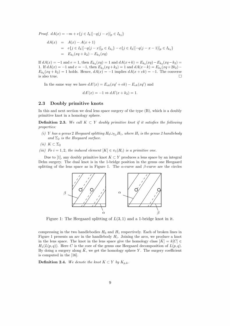
Due to [1], any doubly primitive knot K ⊂ Y produces a lens space by an integralDehn surgery. The dual knot is in the 1-bridge position in the genus one Heegaardsplitting of the lens space as in Figure 1. The α-curve and β-curve are the circles

β

α

α

β

Figure 1: The Heegaard splitting of L(3, 1) and a 1-bridge knot in it.

compressing in the two handlebodies H0 and H1 respectively. Each of broken lines inFigure 1 presents an arc in the handlebody Hi. Joining the arcs, we produce a knotin the lens space. The knot in the lens space give the homology class [K] = k[C] ∈H1(L(p, q)). Here C is the core of the genus one Heegaard decomposition of L(p, q).By doing a surgery along K, we get the homology sphere Y . The surgery coefficientis computed in the [16].

Definition 2.4. We denote the knot K ⊂ Y by Kp,k.

9

2.4 Alexander polynomial of doubly primitive knots.

Ichihara, Saito, and Teragaito gave a formula of the Alexander polynomial of anydoubly primitive knot. This formula works for any doubly primitive knot in anyhomology sphere as well as S3. Here a symbol [[·]]p presents the remainder between 1and p when divided by p.

Theorem 2.2 ([11]). Let K be a doubly primitive knot in a homology sphere Y . Wesuppose that the lens surgery is Yp(K) = L(p, q) and the surgery parameter is (p, k).Then ∆K(t) is computed by the following formula:

∆K(t).=

∑i t

Φ(i)·p−[[q′i]]p·k∑k−1i=0 tk

, (11)

where q′ is the inverse of q in (Z/pZ)× and Φ(i) = #{j ∈ Ik−1|[[q′j]]p < [[q′i]]p}.

Here notice that the right hand side of the formula (11) is not symmetrized. Thecomputation of the Alexander polynomials and the genus for doubly primitive knotsin this paper, we use this formula. We denote the coefficient of the right hand side of(11) by ci.

We define a B-function B : Z2 → Z (or Z → Z) to be B(i, j) = B(i− jk2) = bj−ik

and dB-function dB : Z2 → Z, (or Z → Z) to be

dB(i, j) = dB(i− jk) := bj−ik − bj−(i+1)k.

Lemma 2.2. Let bl be the above coefficients. Then we have

dB(i, j) := bj−ik−bj−(i+1)k =

1 Φ(l) · p− [[q′l]]p · k = j − ik for some l ∈ Ik−1

−1 Φ(l) · p− [[q′l]]p · k = j − 1− ik for some l ∈ Ik−1

0 otherwise.

Thus dB(i, j) = 1 ⇔ dB(i, j + 1) = −1.

Proof. Let F (t) denote the right hand side of (11).

(tk − 1)F (t) =∑i

(bi−k − bi)ti

= (t− 1)k−1∑i=1

tΦ(i)·p−[[q′i]]p·k =k−1∑i=1

(tΦ(i)·p−[[q′i]]p·k+1 − tΦ(i)·p−[[q′i]]p·k)

=∑l

(#{i ∈ Ik−1|Φ(i) · p− [[q′i]]p · k = l − 1} · tl

−#{i ∈ Ik−1|Φ(i) · p− [[q′i]]p · k = l} · tl)

We have, therefore,

bl − bl−k = #{m ∈ Ik−1|Φ(m) · p− [[q′m]]p · k = l} −#{m ∈ Ik−1|Φ(m) · p− [[q′m]]p · k = l − 1}

=

1 Φ(i) · p− [[q′i]]p · k = l for integer i ∈ Ik−1

−1 Φ(i) · p− [[q′i]]p · k = l − 1 for integer i ∈ Ik−1

0 otherwise.

From this formula, the last assertion follows easily.

Here we prove the following:

10

Proposition 2.2. Let K be a doubly primitive knot in a non-L-space homology sphere.Then g(K) ≥ 6 holds. If g(K) = 6, then it is a doubly primitive knot in Σ(2, 3, 7) withsurgery parameter (10, 3).

The knot K10,3 lies in Σ(2, 3, 7) and Σ(2, 3, 7)10(K10,3) = L(10, 1).

Proof. When the slope is p ≤ 9, any doubly primitive knot Kp,k lies in S3 or Σ(2, 3, 5)(see the list in [1] and [17]). Hence, any doubly primitive knot in a non-L-spacehomology sphere satisfies p ≥ 10. From Theorem 1.2, those knots satisfy g(Kp,k) ≥p+12 > 5. From the formula (11), the surgery parameter with g(Kp,k) = 6 is (p, k) =

(10, 3). This example is all the doubly primitive knots in a non-L-space homologysphere 10 ≤ p ≤ 11. Other doubly primitive knots with p ≥ 12 in a non-L-spacehomology sphere have g(Kp,k) ≥ p+1

2 > 6.

The knot K12,5 ⊂ Σ(3, 5, 7), satisfies g(K12,5) = 12 and Σ(3, 5, 7)12(K12,5) =L(12, 11). Here we put the list of doubly primitive knots in non-L-space homologyspheres with the slope p ≤ 23.

p k ZHS g(Kp,k) NSh

10 3 Σ(2, 3, 7) 6 (6, 5, 3, 2, 0)

12 5 Σ(3, 5, 7) 12 (12, 11, 7, 6, 5, 4, 2, 1, 0)

13 5 Σ(3, 5, 8) 14 (14, 13, 9, 8, 6, 5, 4, 3, 1, 0)

15 4 Σ(3, 4, 11) 15 (15, 14, 11, 10, 7, 6, 4, 2, 0)

16 7 Σ(4, 7, 9) 24 (24, 23, 17, 16, 15, 14, 10, 9, 8, 7, 6, 5, 3, 2, 1, 0)

17 3 Σ(2, 3, 11) 10 (10, 9, 7, 6, 4, 2, 1)

17 4 Σ(3, 4, 13) 18 (18, 17, 14, 13, 10, 9, 6, 4, 2, 0)

17 5 Σ(2, 5, 7) 12 (12, 11, 7, 6, 5, 4, 2, 1, 0)

19 3 Σ(2, 3, 13) 12 (12, 11, 9, 8, 6, 5, 3, 2, 0)

20 9 Σ(5, 9, 11) 40 (40, 39, 31, 30, 29, 28, 22, 21, 20, 19, 18, 17,13, 12, 11, 10, 9, 8, 7, 6, 4, 3, 2, 1, 0)

21 8 Σ(5, 8, 13) 42 (42, 41, 34, 33, 29, 28, 26, 25, 21, 20, 18, 17,16, 15, 13, 12, 10, 9, 8, 7, 5, 4, 3, 1, 0)

23 5 Σ(2, 5, 9) 16 (16, 15, 11, 10, 7, 5, 2, 0)

23 7 Σ(2, 3, 11) 13 (13, 12, 10, 9, 6, 5, 3, 2, 0)

Table 1: Doubly primitive knots in non-L-space homology spheres up to p ≤ 23.

Remark 2.1 (Counterexample of Question 1.1). From Table 1 we get the equalities:

NS(K10,3) = NS(T (3, 7)), NS(K12,5) = NS(K17,5) = NS(T (5, 7))

NS(K13,5) = NS(T (5, 8)), NS(K15,4) = NS(T (4, 11))

NS(K17,3) = NS(T (3, 11)), NS(K19,3) = NS(T (3, 13))

NS(K17,4) = NS(T (4, 13)), NS(K20,9) = NS(T (9, 11))

NS(K21,8) = NS(T (8, 13)), NS(K23,5) = NS(T (5, 9)).

Namely, there exist several doubly primitive knots in non-L-space homology sphereswith the same Alexander polynomials as the ones of torus knots. On the other hand,K23,7 is a doubly primitive knot in Σ(2, 3, 11) and the polynomial ∆K23,7 is not acyclotomic polynomial and furthermore, it is not the Alexander polynomial of anyadmissible lens space knot.

11

2.5 Non-zero curves and Alexander region.

We visualize all the non-zero coefficients in A(i, j) and B(i, j) from the values ofdA(i, j) or dB(i, j) in Lemma 2.1 and 2.2.

Lemma 2.3. Let K and X be a knot of type (A) or (B) and A or B respectively.X(i, j) be the X-function of the lens space knot K ⊂ Y with 2g(K) = p. If dX(i, j) = 0and dX(i, j + 1) = 0, then the values of X-function around (i, j) have one of thefollowing local behaviors:

1

0−1

0 −10

10

(e = −1 and X = A or X = B),

−1

j + 1

i

0

1 0

0

−10

1

(e = 1 and X = A)

0

01

1

0 −1

0−1

1

10

0

−1 0

0 −1

j

i+ 1

Definition 2.5 (Non-zero curves). Let K and X be a lens space knot of type (A) or(B) with g(K) = p/2 and X = A or B respectively. We construct curves on R2 asfollows.

(a) Put the integer X(i, j) on each point (i, j) in Z2.

(b) Draw a horizontal arrow on each of the non-zero integers. The direction is theright when A(i, j) = 1 and the left when A(i, j) = −1 as below. Draw an emptyarrow on the zero coefficients.

1 −1 0

(c) Connect the horizontally adjacent arrows with the same direction. Namely, ifthere exist two arrows on (i, j) and (i + 1, j) with the same direction, then weconnect them as below:

1 −11 −1

(d) For (i, j) satisfying dA(i, j+1) = −dA(i, j) = e or dB(i, j) = −dB(i, j+1) = 1,connect the corresponding two non-empty arrows around the point (i, j) as figurebelow. The four patterns are the four possibilities in Lemma 2.3:

1 −10 0

−1 10 0

(X = A and e = −1, or X = B)

−1 00 1

1 00 −1

(X = A and e = 1)

0 1

1 0

0 −1

−1 0

1 0

0 1

−1 0

0 −1j + 1

i

j

i+ 1

Then we can make curves with direction on R2 and call the curves non-zero curves.

12

Notice that on no two points (i, j) and (i+1, j) opposite arrows are drawn, becausethe absolute values of dA(x) are less than 0 or ±1. Furthermore, in the case of X = A,we assume that the curves are periodic.

The curves are weakly-monotonicity about j. If X = A and e = 1, then each ofnon-zero curves are weakly-decreasing about j, and conversely X = A and e = −1 orX = B, then any non-zero curves are weakly-increasing or weakly-decreasing functionabout j.

Lemma 2.4. Let γ be a non-zero curve of type (A) or (B) and p > 1. Each non-zerocurve is simple and does not have end points. In particular, a component of a non-zerocurve is the image of an embedding of R in R2.

The curve is monotone and unbounded about j.

Here an end point means a lattice point that does not connect two lattice pointswith respect to (b) and (c) in Lemma 2.5.

Proof. What the curve is simple is clear from the construction. If the curve has theend, which the point is (i, j) or (i + 1, j), then dA(i, j) implies non-zero. Thus, byusing Lemma 2.1, dA(i + 1, j) = −dA(i, j) or dA(i − 1, j) = −dA(i, j) holds. Thus(i + 1, j) or (i − 1, j) is also end point with opposite direction as (i, j) or (i + 1, j).From the definition of non-zero curve, connecting the two end points smoothly, wecan cancel the two end point. By using cancelation, we can vanish all the possible endpoints as in the figure below. The figures below are examples when e = 1.

⇒

⇒

The second assertion for lens parameter of type (B) is clear. We assume γ is oftype (A). The monotonicity about j is true due to the construction of the non-zerocurve. If the curve is bounded about j, then from the monotonicity, j-value of thecurve is convergent to the an integer. However, since the curve is periodic, the curveis constant. On the line j = j0 ∈ Z, there exists all the coefficients of the Alexanderpolynomial. This implies p = 1. We, therefore, figure out that the γ is unbounded.

The definition of non-zero curve immediately implies the following:

Proposition 2.3. A non-zero curve of type (A) or (B) has symmetry about a pointin R2.

In the end, we can get some symmetric infinte curve with arrow and no end pointson R2. Furthermore, in the case of type (A), any two non-zero curve are congruenteach other by some parallel translation. This will be proven later.

2.6 The case of 2g(K) = p case.

In the case of type (A) and 2g(K) = p we have to consider the behavior of A-functionaround non-trivial dA-function with ag = 2. Since any other coefficients are ±1 or 0,the behaviors of those non-zero coefficients are the same as the case of 2g(K) < p.

Lemma 2.5. Let (p, k) and A(i, j) be a lens space knot K of type (A) with 2g(K) = pand the A-function. If dA(i, j) = 0 and dA(i, j+1) = 0, then the values of A-functionaround (i, j) have one of the following local behaviors:

13

2 1

−1 0

(e = −1),

−1

j + 1

i

0

2 1

(e = 1)

1

−10

j

i+ 1

−1

1

0

i− 1

j + 1

j

i+ 1 i+ 2i

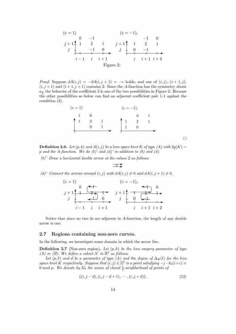
Figure 2:

Proof. Suppose dA(i, j) = −dA(i, j + 1) = −e holds, and one of (i, j), (i + 1, j),(i, j + 1) and (i+ 1, j + 1) contains 2. Since the A-function has the symmetry abouta p

2the behavior of the coefficient 2 is one of the two possibilities in Figure 2. Because

the other possibilities as below can find an adjacent coefficient pair 1, 1 against thecondition (2).

0 1

2 11

1 0 0 1

1

1 0

1 2

(e = −1),(e = 1)

Definition 2.6. Let (p, k) and A(i, j) be a lens space knot K of type (A) with 2g(K) =p and the A-function. We do (b)’ and (d)’ in addition to (b) and (d).

(b)’ Draw a horizontal double arrow at the values 2 as follows:

2

(d)’ Connect the arrows around (i, j) with dA(i, j) = 0 and dA(i, j + 1) = 0.

2 1

−1 0

(e = −1),

−1

j + 1

i

0

2 1

(e = 1)

1

−10

j

i+ 1

−1

1

0

i− 1

j + 1

j

i+ 1 i+ 2i

Notice that since no two 2s are adjacent in A-function, the length of any doublearrow is one.

2.7 Regions containing non-zero curves.

In the following, we investigate some domain in which the arrow lies.

Definition 2.7 (Non-zero region). Let (p, k) be the lens surgery parameter of type(A) or (B). We define a subset N in R2 as follows.

Let (p, k) and d be a parameter of type (A) and the degree of ∆K(t) for the lensspace knot K respectively. Suppose that (i, j) ∈ Z2 is a point satisfying −j−k2(i+c) ≡0 mod p. We denote by N0 the union of closed 1

2 -neighborhood of points of

{(i, j − d), (i, j − d+ 1), · · · , (i, j + d)}. (12)

14

Let (p, k) and d be a parameter of type (B) and the top degree of ∆Kp,krespectively.

For a fixed integer j ∈ Z there exists (i, j) ∈ Z2 such that

{(i, j − d), (i, j − d+ 1), · · · , (i, j + d)}

contains all the non-zero coefficients. We denote by N0 the union of closed 12 -neighborhood

of these points.In both cases, let Nl denote {(x+ l, y−k2l) ∈ R2|(x, y) ∈ N0}, which is the parallel

translation of N0 by (l,−k2l) on R2. We call the region

N = ∪l∈ZNl

an non-zero region.

Here we define closed ϵ-neighborhood of (i′, j′) to be {(x, y) ∈ R2| |x−i′|+|y−j′| ≤ϵ}. In the case of type (A), changing the choice of (i, j) satisfying −j − k2(i + c) ≡0 mod p, we get another non-zero region. An non-zero region N is connected due to−p/2 < k2 < p/2.

Lemma 2.6. Let K be a lens space knot of type (A) and (B). Then any connectedcomponent of non-zero curves is contained in a non-zero region,

Proof. Suppose that (p, k) be a lens space surgery of type (B). Since all the non-zerocoefficients are contained in the non-zero region, the non-zero curve is also containedin the non-zero region.

Let (p, k) be a lens space surgery of type (A) with e = −1. Suppose that a non-zerocurve γ is passing on two non-zero regions N and N ′ as in Figure 3. Let s be thevertical segment in which γ traverses ∂N ∩ ∂N ′. We assume that the curve γ meetsat the highest meeting point on s and at the meeting point the direction is from leftto right. See Figure 3. If the left 1 is not the top coefficient of ∆K(t), then from the

N ′

N

11γ

sN ′

N

11γ

−1

δ s′

−1

Figure 3: A non-zero curves passing two non-zero region.

alternating condition of ∆K , the next above non-zero coefficient is −1. Let δ be thenon-zero curve on that −1. Actually, the curve δ agrees with γ. In fact, if the curve δis not γ, then from the monotonicity and unboundedness about j (Lemma 2.4), δ andγ have to meet at least a point as in Figure 3. Hence, we have δ = γ.

Suppose that the curve γ meets on the next segment s′. The left of the meetingpoint is−1. In the shaded region of the right in Figure 3 there is no non-zero coefficient.This contradicts the fact that the top coefficient of the Alexander polynomial is 1.

Suppose that the left 1 is the top coefficient of ∆K(t). Let N ′1 be a non-zero part

{(x+1, y−k2−p) ∈ R|(x, y) ∈ N0}, which is the right below non-zero part of N1. Forthe assumption to be true, we have to have −k2 − p ≥ 0. This case does not occur.

15

Suppose that γ is passing from right to left as in Figure 4. We may assume themeeting point is the heighest one among such meeting points. Then the next abovenon-zero coefficient is 1, however, we cannot draw a curve passing the point. Becausethe curve passing the coefficient 1 have to agree with γ, which is passing from the leftto the right at a point in the segment. From what we proved above, such curve doesnot exist.

N ′

N

−1−1γ

s

N ′

N

−1−1γ

s

⇒ 1

Figure 4: A part of non-zero curves passing two non-zero region from right to left.

In the case of e = 1, since the argument is parallel by the mirror image about thej-axis, then the same assertion holds.

Hence, any non-zero curve is contained in the non-zero region.

Lemma 2.7. Let K be a lens space knot of type (A). Then, the i-coordinate of anynon-zero curve is unbounded both above and below.

Proof. Suppose that e = −1. Let γ be a non-zero curve in a non-zero region N . If γis bounded above by i = i0. Let j0 be the minimal integer in A∩{i = i0}. The latticepoints on R := A∩ {i ≤ i0 +

12} ∩ {j ≥ j0 − 1

2} is finite. Once the curve γ enter in R,the curve does not go out from R. This contradicts the fact that the lattice points inR are finite. Thus the curve γ is unbounded above about i.

In the case of e = 1, the argument of the proof is the mirror image or the case ofe = −1 about the j-axis.

The unboundedness about i of the non-zero curve of type (B) is clear from theconstruction of the non-zero region N .

Theorem 2.3 (Traversable Theorem). Let (p, k) be a lens surgery parameter of type(A) or (B). The non-zero curves which are contained in each non-zero region have asingle connected component.

Proof. Suppose that two connected components γ and δ of non-zero curves are con-tained in a non-zero region. Since γ and δ are disjoint each other, we may assumethat one of three components in R2 − γ − δ does not have any non-zero componentand γ is upper of δ. We can find a not-alternating pair 1 and 1 in ∆K(t) as seen inFigure 5 (the case of e = −1). If you cannot find not-alternating coefficients, then γand δ must be separated by a vertical line i = x0 for a real number x0. However, fromLemma 2.7 any non-zero curve is unbounded about the i-coordinate.

Thus, we can get the inequality.

Corollary 2.1. Let (p, k) be a lens space surgery of type (A). Then an inequalitymax{k, |k2|} ≤ 2g(K) + 1 holds.

16

Two non-zero coefficients which are not allowed.

γ

δ

Figure 5: The case of e = −1.

Proof. By exchanging k and |k2|, we assume that k ≤ |k2|. Let N = ∪i∈ZNi be anon-zero region. If |k2| ≥ 2g(K) + 2, then by the translation (1,−k2), Ni and Nj

(i = j) are disconnected. Thus, the non-zero region is infinite disjoint union of N0.Since Ni has at most finite lattice points, we cannot embed any non-zero curve passinginfinite non-zero coefficients. This contradicts Theorem 2.3.

Corollary 2.2. Let (p, k) be a lens surgery parameter of type (A). If k ≤ |k2| and2g(K) ≤ |k2| ≤ 2g(K)+1, then we have e = −1, ∆K(t) = ∆T (2,2d+1) and (p, k, |k2|) =(4d+ 1, 2, 2d) or (4d+ 3, 2, 2d+ 1).

There exists no lens surgery with |k2| = 2g(K)− 1.

Proof. Let (p, k) be a lens surgery parameter of type (A). If |k2| = 2d + 1, then bythe translation (1,−k2) = (1,−e(2d + 1)) two adjacent non-zero regions N0 and N1

meet one corner point. Then, we can embed a non-zero curve as in Figure 6. Hence,naturally all the lattice points in the non-zero region Ni have non-zero coefficients.Thus we have

∆K(t) = td − td−1 + td−2 − · · ·+ t−d.

Suppose that d > 1. Then if p > 2(2d+ 1) + 1, then the dA-function has adjacenttwo 0s on the line i = i0. This contradicts that there exists an adjacent pair (1,−1)and (−1, 1) of dA-function in order on the line with respect to e = 1 or e = −1respectively. This is equivalent to p < 3|k2|. Thus we have p = 2(2d + 1) + 1 or2(2d+ 1). Since gcd(p, k) = 1, p = 4d+ 3 and e = −1.

Suppose that d = 1. Then ∆K(t) = t− 1+ t−1 holds. The only lens surgery is thetrefoil knot surgery with (p, k) = (7, 2), k2 = −3 and e = −1 (see [15]).

If |k2| = 2d, then the non-zero region becomes as in Figure 7. Since the non-zerocurve is connected in the region, other lattice points in the region are all non-zero.This means that ∆K(t) = ∆T (2,2d+1)(t). Furthermore, in the same as above, we havep < 3|k2|. Thus we have p = 4d+1, 4d+2. Since gcd(p, |k2|) = 1, we have p = 4d+1.

If |k2| = 2g(K) − 1, then since the coefficients ag and ag−1 are adjacent in theplane, there exists a value ±2 in the dA-function. This is contradiction.

Corollary 2.3. Let K be a lens space knot in Y of type (A) with surgery parameter(p, k). If ∆K(t) = ∆T (2,2m+1)(t), then we have max{k, |k2|} ≤ 2g(K)− 2.

17

T0

T−1

T1

Figure 6: The case of e = −1 with |k2| = 2d+ 1.

11

11

11

11

−1

1

−1⇒ ⇒

Figure 7: The case of e = −1.

18

Proof. From Corollary 2.2, the required assertion holds.

3 The coefficients of X(i, j).

3.1 The second term n2 and adjacent region.

The aim of this section is to prove the main theorem. First we prove the following

Proposition 3.1. Let K be a nontrivial lens space knot of type (A) or (B). Supposethat (p, k) be a surgery parameter of K. Then n2 = d− 1 holds.

Proof. Let K be a lens space knot of type (A) or (B) and (p, k) the surgery parameterof K. Suppose that e = −1. Let N be the non-zero region and (i, j) ∈ N the bottompoint the fixed i = i0. The point (i0, j) has the right arrow. Since |k2| > 1 and thetraversable theorem, the lattice point next to (i0, j) must be (i0, j+1). Thus (i0, j+1)has left arrow, that is, ag−1 = −1. In the case of e = 1, the same argument followsag−1 = −1.

1N

(i0, j)

1N

(i0, j)

⇒ −1

Figure 8: The case of e = −1.

This theorem implies Theorem 1.3. Next, we prove Theorem 1.5

Proof of Theorem 1.5. Suppose that e = 1. In the case of e = −1 the proof is themirror image with orientation reversing of the non-zero curve about the j-axis. Let sbe a vertical left segment in ∂N . Let (i0, j0) be a lattice point satisfying (i0, j0− e

2 ) ∈ sand X(i0, j0) = 1. Then, the non-zero curve passing (i0, j0) connects (i0−e, j0+1) or(i0, j0+1) since it is contained in the non-zero region. If (i0− e, j0+1) ∈ N , then theformer case holds. If (i0− e, j0+1) ∈ N , then the latter case holds and (i0− e, j0+1)corresponds to the bottom term t−g. See the figure below.

Thus, on the right lattice points of the segment s are contained in the adjacentregion. Hence, we have α ≥ |k2| − 1. Exchanging the k and |k2|, we have α + 1 ≥max{k, |k2|}.

N(i0, j0)

s

N(i0, j0)

a−g

19

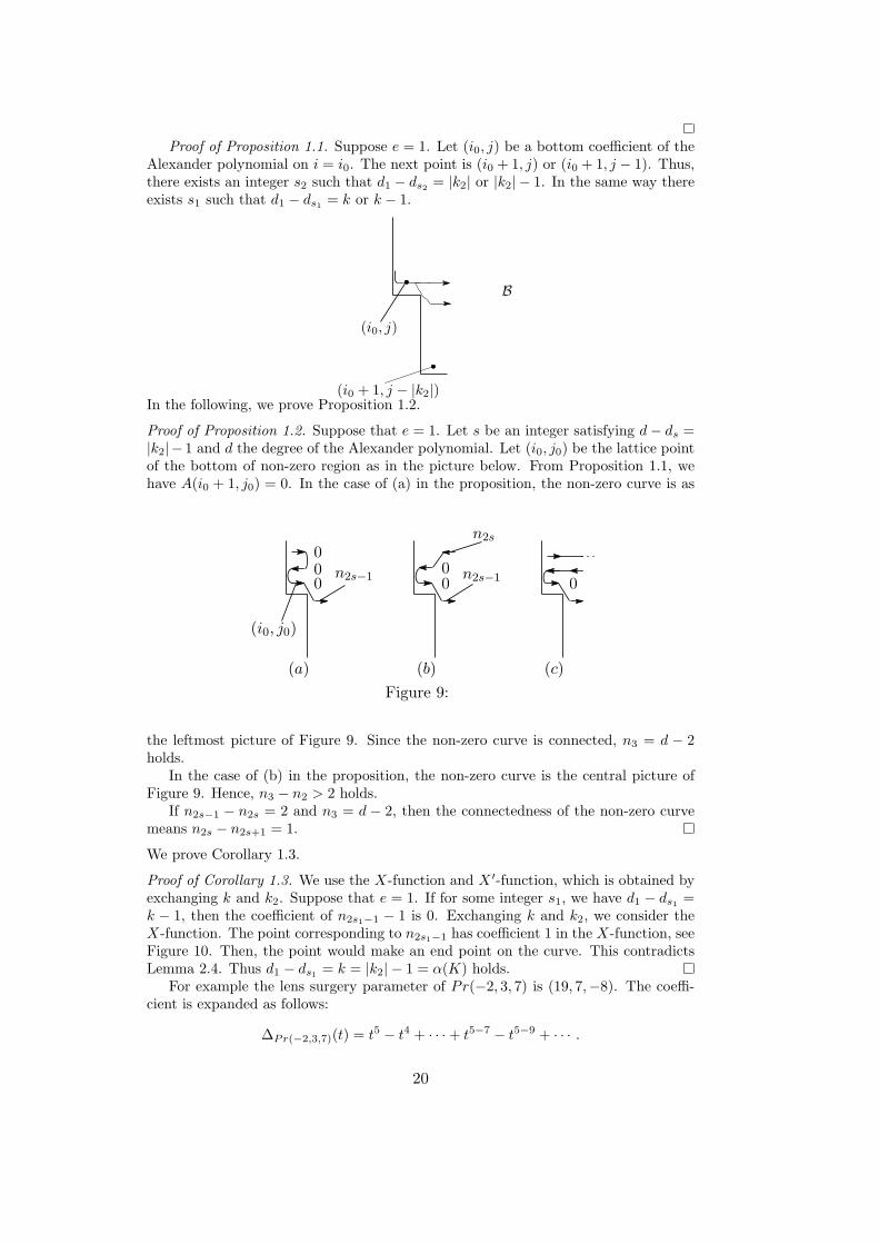
Proof of Proposition 1.1. Suppose e = 1. Let (i0, j) be a bottom coefficient of theAlexander polynomial on i = i0. The next point is (i0 + 1, j) or (i0 + 1, j − 1). Thus,there exists an integer s2 such that d1 − ds2 = |k2| or |k2| − 1. In the same way thereexists s1 such that d1 − ds1 = k or k − 1.

B

(i0, j)

(i0 + 1, j − |k2|)In the following, we prove Proposition 1.2.

Proof of Proposition 1.2. Suppose that e = 1. Let s be an integer satisfying d− ds =|k2|− 1 and d the degree of the Alexander polynomial. Let (i0, j0) be the lattice pointof the bottom of non-zero region as in the picture below. From Proposition 1.1, wehave A(i0 + 1, j0) = 0. In the case of (a) in the proposition, the non-zero curve is as

0

(i0, j0)

0 0

(a) (b) (c)

000

n2s−1

n2s

n2s−1

Figure 9:

the leftmost picture of Figure 9. Since the non-zero curve is connected, n3 = d − 2holds.

In the case of (b) in the proposition, the non-zero curve is the central picture ofFigure 9. Hence, n3 − n2 > 2 holds.

If n2s−1 − n2s = 2 and n3 = d − 2, then the connectedness of the non-zero curvemeans n2s − n2s+1 = 1.

We prove Corollary 1.3.

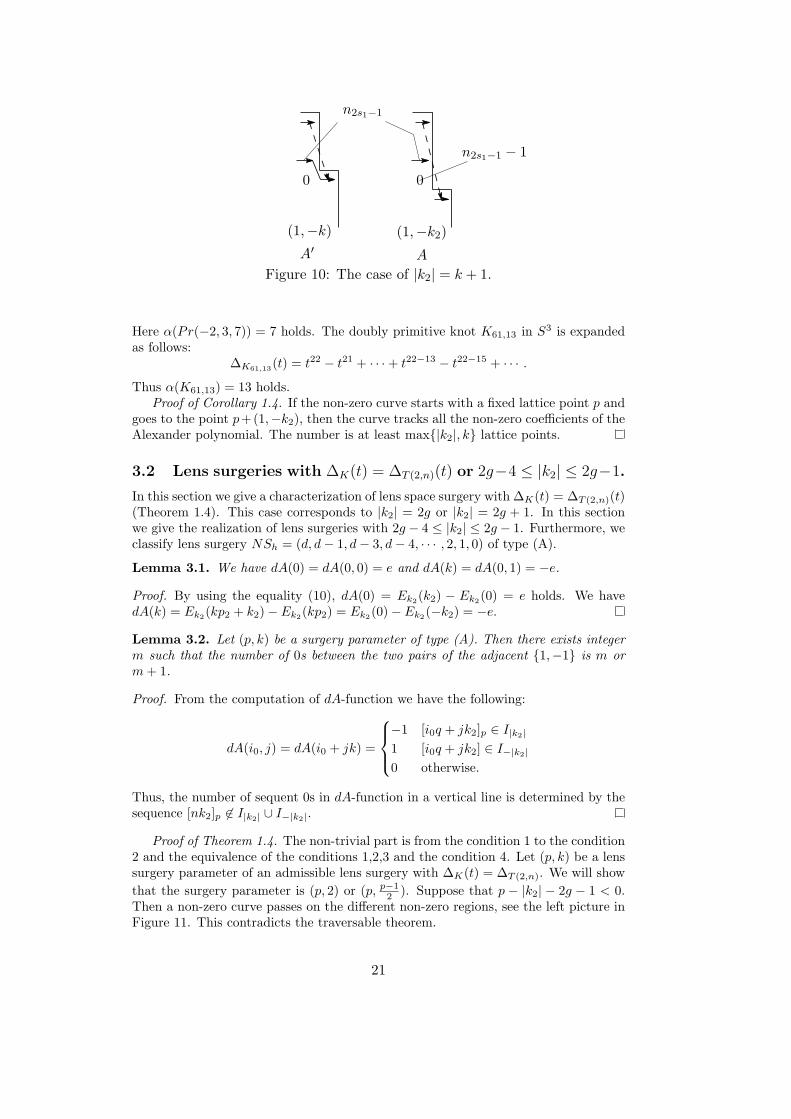
Proof of Corollary 1.3. We use the X-function and X ′-function, which is obtained byexchanging k and k2. Suppose that e = 1. If for some integer s1, we have d1 − ds1 =k − 1, then the coefficient of n2s1−1 − 1 is 0. Exchanging k and k2, we consider theX-function. The point corresponding to n2s1−1 has coefficient 1 in the X-function, seeFigure 10. Then, the point would make an end point on the curve. This contradictsLemma 2.4. Thus d1 − ds1 = k = |k2| − 1 = α(K) holds.

For example the lens surgery parameter of Pr(−2, 3, 7) is (19, 7,−8). The coeffi-cient is expanded as follows:

∆Pr(−2,3,7)(t) = t5 − t4 + · · ·+ t5−7 − t5−9 + · · · .

20

0

(1,−k2)

0

(1,−k)

A′ A

n2s1−1

n2s1−1 − 1

Figure 10: The case of |k2| = k + 1.

Here α(Pr(−2, 3, 7)) = 7 holds. The doubly primitive knot K61,13 in S3 is expandedas follows:

∆K61,13(t) = t22 − t21 + · · ·+ t22−13 − t22−15 + · · · .

Thus α(K61,13) = 13 holds.Proof of Corollary 1.4. If the non-zero curve starts with a fixed lattice point p and

goes to the point p+(1,−k2), then the curve tracks all the non-zero coefficients of theAlexander polynomial. The number is at least max{|k2|, k} lattice points.

3.2 Lens surgeries with ∆K(t) = ∆T (2,n)(t) or 2g−4 ≤ |k2| ≤ 2g−1.

In this section we give a characterization of lens space surgery with ∆K(t) = ∆T (2,n)(t)(Theorem 1.4). This case corresponds to |k2| = 2g or |k2| = 2g + 1. In this sectionwe give the realization of lens surgeries with 2g − 4 ≤ |k2| ≤ 2g − 1. Furthermore, weclassify lens surgery NSh = (d, d− 1, d− 3, d− 4, · · · , 2, 1, 0) of type (A).

Lemma 3.1. We have dA(0) = dA(0, 0) = e and dA(k) = dA(0, 1) = −e.

Proof. By using the equality (10), dA(0) = Ek2(k2) − Ek2(0) = e holds. We havedA(k) = Ek2(kp2 + k2)− Ek2(kp2) = Ek2(0)− Ek2(−k2) = −e.

Lemma 3.2. Let (p, k) be a surgery parameter of type (A). Then there exists integerm such that the number of 0s between the two pairs of the adjacent {1,−1} is m orm+ 1.

Proof. From the computation of dA-function we have the following:

dA(i0, j) = dA(i0 + jk) =

−1 [i0q + jk2]p ∈ I|k2|

1 [i0q + jk2] ∈ I−|k2|

0 otherwise.

Thus, the number of sequent 0s in dA-function in a vertical line is determined by thesequence [nk2]p ∈ I|k2| ∪ I−|k2|.

Proof of Theorem 1.4. The non-trivial part is from the condition 1 to the condition2 and the equivalence of the conditions 1,2,3 and the condition 4. Let (p, k) be a lenssurgery parameter of an admissible lens surgery with ∆K(t) = ∆T (2,n). We will show

that the surgery parameter is (p, 2) or (p, p−12 ). Suppose that p − |k2| − 2g − 1 < 0.

Then a non-zero curve passes on the different non-zero regions, see the left picture inFigure 11. This contradicts the traversable theorem.

21

−11−11

N ′N

N ′

N

Figure 11: The case of p− |k2| − 2g − 1 < 0 and p− |k2| − 2g − 1 ≥ 0.

Hence we have p−|k2|−2g−1 ≥ 0 (see the right picture in Figure 11). Then thereexists x ∈ Z such that dA(x) = e, dA(x+ k) = −e, dA(x+2k) = e, · · · , dA(x+(|k2| −1)k) = −e, in particular k2 is an even integer or |k2| = 2g+1. See Figure 12. If 4 ≤ |k2|,then the number of 0s between two vertical pairs of {1,−1} in the dA-function mustbe zero or one. Namely, we have p < 3|k2| and p = |k2|+ 2g + 1 or p = |k2|+ 2g + 2.Hence |k2| = 2g or 2g + 1 holds. This implies the proof from the condition 1 tothe condition 4. The only possibilities are (p, |k2|) = (4g + 1, 2g), (4g + 3, 2g + 1) inFigure 13. Hence, we have e = −1 and |k2| = p−1

2 .If |k2| < 4, then |k2| = 2 holds. In this case, we have 2k = |k2|k < p and

k|k2| = p− 1 holds. Thus, we have k = p−12 .

If (p, k) is a lens surgery parameter with the condition 4, then the Alexanderpolynomial is the same as the one of T (2, 2d+ 1). This proves from 4 to from 1.

Corollary 3.1. If a lens space knot K with |k2| = 2g(K), then (p, k) = (5, 2). Inparticular K is the trefoil knot.

Proof. Let (p, k) be a lens surgery parameter with |k2| = 2g(K). Since there existsno case of |k2| ≥ 4 from the proof of the previous theorem, we have |k2| = 2 = 2g(K).Thus g(K) = 1 holds. The genus one case is classified in [3]. The knot is the trefoil.

Let (p, k) be a surgery parameter and k2 = [k−1]p. We classified lens surgerieswith 2g(K) ≤ |k2|. Here we discuss further classification.

Proposition 3.2. There exists no lens space knot with 2g(K)− 1 = |k2|.If a lens space knot K satisfies 2g(K) − 2 = |k2| and g(K) < p−1

2 , then the onlysurgery parameters are (19, 7) or (11, 3). The Alexander polynomials are

∆K(t) = ∆Pr(−2,3,7)(t), or ∆K(t) = ∆T (3,4)(t).

respectively.

Proof. In the case of 2g(K) − 1 = |k2|, the coefficients ag = 1 and ag−1 = −1 isadjacent on the horizontal line j = j0.

22

0

The A-function.

0

The dA-function.

1−11−1000

−11−1

Figure 12: The case of p = |k2|+2g+2. The three 0s contradict the fact that the numberof 0s between the pairs of {1,−1} is zero or one.

The (p, |k2|) = (4g + 3, 2g + 1) case. The p = |k2|+ 2g(K) + 1 case.

0

0

Figure 13: The case of p = |k2|+ 2g + |k2|+ 1.

23

In the case of 2g(K)−2 = |k2|, the non-zero sequence isNSh = (d, d−1, d−2, · · · , 0)or (d, d− 1, d− 3, d− 4, · · · , 2, 1, 0).

The former case corresponds to the surgery parameter (p, 2) due to Theorem 1.4.We consider the latter case. Let (p, k) be a surgery parameter with |k2| = 2g − 2. Inthe case of g ≥ 5, the number of sequent 0s on a line of dA is 0 or 1 (Lemma 3.2).

By Lemma 3.2, we have p − |k2| = 2g + 1 and p − |k2| = 2g + 2. Thus, we have(p, |k2|) = (4g − 1, 2g − 2). The case (4g, 2g − 2) is ruled out since gcd(p, k) = 1. SeeFigure 14 (for e = −1) and Figure 15 (for e = 1).

The lengths between the 3 0-values in a vertical line in dA-function are 5, 2g − 3and 2g − 3 see Figure 14. Thus, k = 2g − 3 holds. Therefore, we have k|k2| =(2g − 3)(2g − 2) = 4g2 − 10g + 6 ≡ 3g + 3 ≡ ±1 mod p. This means 3g + 3 = 4g − 2,that is, (p, k) = (19, 7) and g = 5. This case is realized by the (−2, 3, 7)-pretzel knot.

In the case of g < 5, we have g = 3 and (p, k) = (11, 3) see Figure 16.

0

0

0

0

0

−1

−1

0

A-function. dA-function.

1

01

0

1

1

1−1...

10

−1

−1

1−1

1−1

−110

5

2g − 3

1−10

2g − 3

Figure 14:

Proposition 3.3. If a lens space knot K satisfies 2g(K)−3 = |k2| and type (A), thenthe only surgery parameter is (11, 4) and

∆K(t) = t3 − t2 + 1− t−1 + t−2 + t−3

This surgery can be realized by the (3, 4)-torus knot.

Proof. From the condition 2g(K)− 3 = |k2|, the Alexander polynomial is

NSh(K) = (d, d−1, d−3, d−4, · · · , 2, 1, 0) =: N1 or (d, d−1, d−4, d−5, · · · , 2, 1, 0) =: N2.

If p− |k2| < 2g + 1holds, then the case of NSh = N1 holds and the A-function is thepicture (a) in Figure 17. This picture has periodicity 2 for the i-direction. Thus p = 2holds. This case does not occur. Hence p− |k2| ≥ 2g + 1 holds.

Suppose that p− |k2| ≥ 2g + 1. If NSh = N1, then the dA-function is the picture(b). This picture is inconsistent with Lemma 3.2. If NSh = N2 and g ≥ 5, thenthe nubmer m in Lemma 3.2 is 0. Thus p − |k2| = 2g + 1 or 2g + 2, therefore,(p, k) = (4g−2, 2g−3), (4g−1, 2g−3). The number of 0-values in a vertical sequenct

24

0

0

0

0

−1

0

1

A-function. dA-function.

−1

1

1−1...

−1

10

10

...

5

2g − 3

2g − 3

10

−110

−1

Figure 15:

A-function.

0

0

0

00

0

0

0

00

dA-function.

0

−1

1−1

1

10

0

−1

1−1

1

10

0

−1

1−1

1

10

0

−1

1−1

1

10

0

−1

1−1

1

10

0

−1

1−1

1

10

−101−1

1−1

0−1

−101−1

Figure 16: The A-function or dA-function of the (3, 4)-torus knot.

25

p point in dA-function is 5 or 4 respectively. The lengths of the 5 0-values in a verticalline in dA-function are 2g − 6, 3, 3, 2g − 5, and 3. Here, the existence of the length 3implies 3|k2| − p = 2g + 8 ≤ 4. However this is contradiction of the condition g ≥ 5.In the similar way, the case of p = 4g − 1 does not occur.

If NSh = N2 and g < 5, then g = 3 and the A-function is Figure 18. Sincethe case of p − |k2| < 2g + 1 does not occur, p − 3 = 8, 9, or 10. Thus we have(p, |k2|) = (11, 3), (13, 3) due to gcd(p, |k2|) = 1. This case NSh = (3, 2, 0) is realizedby the torus knot T (3, 4).

0

00

0

The 2g(K)− 3 = |k2| case.

000

000

000

0

00

(a)

(b)

A-function

100

−1

1−1

dA-function

1−1−11

Figure 17: The A-function or dA-function.

00

0

1

The A-function. The dA-function.

−10

0

01−100 0

1−10

1−10

0−11

Figure 18: The A-function or dA-function in the case of NSh = N2 and g = 3.

Proposition 3.4. If a lens space knot K of type (A) satisfies 2g(K)− 4 = |k2|, thenthe only surgery parameter is (19, 8) and ∆K(t) = ∆Pr(−2,3,7)(t).

The proof can be done by the similar method to Proposition 3.3, hence, we omitit.

Proposition 3.5. The only lens space knot K whose half non-zero exponent is (g, g−1, g − 3, g − 4, · · · , 3, 2, 1, 0) is g = 3, 5. This case can be realized by the (3, 4)-torusknot and (−2, 3, 7)-pretzel knot respectively.

Proof. We suppose the case of 2g − 4 < |k2|. The only case is |k2| = 2g − 5, seeFigure 19.

Suppose that g ≥ 5. Since p−|k2| < 2g+1 contradicts the traversable theorem, wemay assume p− |k2| ≥ 2g + 1. However, the values are inconsistent with Lemma 3.2see the right of Figure 19.

26

00

|k2| = 2g − 5

−1

001

00

1−101−11

Figure 19:

If g ≤ 4, then |k2| < 2g − 4. This contradicts the assumption.Thus, |k2| ≤ 2g−4 holds. The case is already classified in the previous proposition.

Such lens surgeries are realized by T (3, 4) or Pr(−2, 3, 7).

Proof of Theorem 1.6. If (n1, n2, n3, n4) = (d, d − 1, d2, d2 − 1), (d, d − 1, d2, d2 −2), (d, d− 1, d2, d2 − 3), then by using Proposition 1.2, n3 = n2 + 1 holds.

We suppose the type (A). If p − |k2| ≥ 2g + 1, then the number in Lemma 3.2 is0. Thus |k2| = 3 or 4 holds. The left two pictures in Figure 20 are non-zero curves of|k2| = 3 or 4. However, each of picture does not describe the non-zero curve of lenssurgery. Because, in the case of |k2| = 3, we cannot connect the curve as a connectedcurve and in the case of |k2| = 4, the curve does not have a symmetry about a point(Proposition 2.3).

If p− |k2| < 2g+1, then the right picture is the non-zero curve. Since the numberm in Lemma 3.2 is 0, then p = 2g + 1 or 2g + 2. These cases are not type (A).

0

00

0

00

0

00

0

00

|k2| = 3 |k2| = 4

000

00

00

00

00

p− |k2| > 2g + 1.p− |k2| ≤ 2g + 1.

Figure 20: The case of (n1, n2, n3, n4) = (d, d− 1, d2, d2 − 3) and |k2| = 3 or 4.

27

3.3 Lens surgeries with g(K) ≤ 5 or with at most 7 non-zerocoefficients.

Before the classification of lens space surgery of g(K) ≤ 5 or at most 7 non-zerocoefficients, we characterize the lens surgery of torus knot surgery.

Proposition 3.6. We consider any admissible lens surgery with surgery parameter(p, k, |k2|) (k ≤ |k2|). Let γ be a non-zero curve and γ′ the non-zero curve obtained bythe (k,−1) parallel translation. Then, the parameter (p, k) can be realized by a surgeryparameter of a torus knot surgery in S3, if and only if the interior of the strip betweenγ and γ′ does not contain any other non-zero curve.

Proof. The parallel translation by a vector v1 = (1,−k2) gives a self-congruence mapon non-zero regions, due to the definition of the non-zero region. The lattice pointsmoved by this translation lie in the same non-zero region. The vector v2 = (0,−p)gives a congruence map to the just right non-zero region. Thus kv1−mv2 = (k,−kk2+mp) = (k,−1) give a congruence map to the |m|-th non-zero region on the right, wherem is an integer defined by m = kk2−1

p . If (p, k) is the lens surgery parameter of atorus knot surgery, then we have p = kek2 − e = emp and m = e. Hence the strip oftwo non-zero curves γ, γ′ does not contain the other non-zero curves.

Corollary 2.2, Corollary 2.3 and Proposition 3.6 can easily give a classification ofnon-torus polynomial with lens space surgeries with small Seifert genus.

Here we demonstrate the classification of ∆K(t) of lens space knot when small kand |k2|, or small g(K) = d. First, if k = 1, then k2 = 1 holds, hence ∆K(t) = 1. Ifk = 2, then we classified in Theorem 1.4.

In the case of g ≤ 3, all the lens surgery polynomials are torus polynomials. Thetorus knots with g(K) = 4 are T (2, 9) and T (3, 5). Other admissible lens space knotswith g = 4 are the following:

Proposition 3.7. Let (p, k, |k2|) be a lens surgery parameter of (A) with k ≤ |k2|. Ifg = 4, then any lens surgery polynomial is torus knot polynomial.

Proof. We may assume 3 ≤ k ≤ |k2|. In the case of g = 4, the possible half non-zero sequence of non-torus polynomials is (4, 3, 2, 0). The sequences (4, 3, 1, 0) and(4, 3, 2, 1, 0) present torus knot polynomials. The (4, 3, 0) case fails to Theorem 20.

From Corollary 2.3 |k2| ≤ 6 holds. If |k2| = 6, then the lens surgery polynomialis ∆T (2,7) or ∆T (3,5) only. We assume |k2| ≤ 5. Since the surgery slope p satisfiesp ≥ 2g(K) and is the divisor of k|k2| ± 1 less than k|k2| ± 1, the only possibility is(p, k) = (8, 3). The half non-zero sequence is (4, 3, 1, 0) = NSh(T5,3).

(8, 3) can be realized by a doubly primitive knot in the Poincare homology sphere[16] and has non-zero sequence NSh(K8,3) = NSh(K14,3). The sequence (4, 3, 0) doesnot present any admissible lens surgery knot polynomial.

The author proved in [15] the following:

Theorem 3.1 (Theorem 16 in [15]). If a knot K satisfying ∆K(x) = xn − 1 + x−n

admits lens surgery, then n = 1 and moreover K is the trefoil knot.

This theorem was proved by a longer argument of coefficients, however, it is acorollary of Theorem 1.3. We more argue the relation between the number of non-zero coefficients of the Alexander polynomial and lens surgery.

The polynomial tn − tn−1 + 1 − t−n+1 + t−n satisfies the condition n2 = d− 1 inTheorem 1.3, however, not all the polynomials are lens surgery polynomials.

28

Corollary 3.2. If the Alexander polynomial ∆K(t) of lens space knot of type (A) or(B) has 5 non-zero coefficients, then ∆K(t) = ∆T (5,2)(t), or ∆T (4,3)(t).

In other words, if the lens surgery polynomial is of form tn−tn−1+1−t−n+1+t−n,then n = 2, 3 holds.

This type of polynomial is not given from a doubly primitive knot in any non-L-space homology sphere.

Proof. The case of type (A) is a corollary of Theorem 1.6. In the case of type (B)and (n1, n2, n3, n4) = (d, d− 1, d2, d2 − 3), we have g(K) = 4. However the genus of adoubly primitive knot in a non-L-space homology sphere is g(K) ≥ 6. This case doesnot occur.

Corollary 3.3. Admissible lens space knots with g = 5 are T (2, 11) and Pr(−2, 3, 7).

Here Pr(p, g, r) is the (p, q, r)-pretzel knot.

Proof. From Corollary 2.3, since 3 ≤ k ≤ |k2| ≤ 8 holds, the parameters (p, k) sat-isfying mp = kk2 − 1 with |m| ≥ 2 are (11, 3), (13, 5), (17, 5), (18, 5), (19, 7). Theadmissible parameters among these are (11, 3), (18, 5), (19, 7), and (22, 3). Thus,K11,3 = T (3, 4), T18,5 = T19,7 = Pr(−2, 3, 7) and g(K22,3) = 11 holds.

The non-zero sequences of these knots T (2, 11) and Pr(−2, 3, 7) are (5, 4, 3, 2, 1, 0)and (5, 4, 2, 1, 0).

The next classification is lens space knot with the 7 non-zero coefficients.

Corollary 3.4. If the Alexander polynomial ∆K(t) of lens space knot of type (A) or(B) has 7 non-zero coefficients, then ∆K(t) = ∆T (7,2)(t), ∆T (5,3)(t), or ∆T (4,5)(t).

If K is a lens space knot of type (A) or (B) with

∆K(t) = tn − tn−1 + t− 1 + t−1 − t−n+1 + t−n (13)

∆K(t) = tn − tn−1 + t2 − 1 + t−2 − t−n+1 + t−n, (14)

then when (13), n = 4, 5 and when (14), n = 6.

Proof. If the lens surgery polynomial is (13), by describing the non-zero curve, we findg(K) ≤ 5. Thus n = 5 or 4.

If the lens surgery polynomial is (14), The possibilities of non-zero curves are thepictures in Figure 21. The next is the table of the 4 non-zero curves.

|k2| p α4 6 45 7 55 6 44 5 3

By using the inequality (6) in Theorem 1.5, considering all the cases (p, k, |k2|), weget (p, |k2|, g) = (19, 4, 6), (21, 4, 6) and ∆K(t) = ∆T4,5(t). These cases corresponds to

The next classification of admissible lens surgeries is the surgeries with 9 non-zerocoefficients. This is left for readers.

29

0

0

00

0

0

00

0

0

00

00

00

000

0

0000

0

0

0

00

000

0

0

000

00

0

0

00

00

0

0

00

00

0

0

0

0

0

0

0

0

0

0

0

0

0

0

Figure 21: The cases of (|k2|, g) = (4, 6), (5, 7), (5, 6), (4, 5) respectively.

Problem 3.1. Classify the Alexander polynomial with 9 non-zero coefficients. Thepolynomials are of the form:

tn − tn−1 + tm − tm−1 + 1 + t−m − t−m+1 − t−n + tn

ortn − tn−1 + tm − tm−2 + 1 + t−m − t−m+2 − t−n + tn.

3.4 Examples

In Table 2 and 3 we list doubly primitive knots with g(K) ≤ 30 in non-L-spacehomology spheres.

References

[1] J. Berge, Some knots with surgeries yielding lens spaces, unpublishedmanuscript.

[2] S. A. Bleiler and R. A. Litherland, Lens spaces and Dehn surgery, Proc. Amer.Math. Soc. 107 (1989), no. 4, 1127-1131.

[3] H. Goda and M. Teragaito, Dehn surgeries on knots which yield lens spaces andgenera of knots, Math. Proc. Cambridge Philos. Soc. 129 (2000), 501-515.

[4] J. Greene, L-space surgeries, genus bounds, and the cabling conjec-ture,arXiv:1009.1130v2

[5] J. Greene, The lens space realization problem, Annals of Mathematics 177 (2):449511

[6] D. Krcatovich, A restriction on the Alexander polynomials of L -space knots,arXiv:1408.3886

[7] T. Kadokami, and Y. Yamada,A deformation of the Alexander polynomials ofknots yielding lens spaces, Bull. of Austral. Math. Soc.

[8] M. Hedden, T. Watson, On the geography and botany of knot Floer homology,arXiv:1404.6913

30

g p k |k2| NSh, AS α

6 10 3 3 (6, 5, 3, 2, 0) 6(6, 3, 0)

10 17 3 6 (10, 9, 7, 6, 4, 3, 1, 0) 11(10, 7, 4, 1,−1)

12 12 5 5 (12, 11, 7, 6, 5, 4, 2, 1, 0) 14(12, 7, 5, 2, 0,−2)

12 17 5 7 (12, 11, 7, 6, 5, 4, 2, 1, 0) 14(12, 7, 5, 2, 0,−2)

12 19 3 6 (12, 11, 9, 8, 6, 5, 3, 2, 0) 12(12, 9, 6, 3, 0)

13 23 7 10 (13, 12, 10, 9, 6, 5, 3, 2, 0) 13(13, 10, 6, 5, 3, 0)

14 13 5 5 (14, 13, 9, 8, 6, 5, 4, 3, 1, 0) 15(14, 9, 6, 4, 1,−1)

15 15 4 4 (15, 14, 11, 10, 7, 6, 4, 2, 0) 11(15, 11, 7, 4)

16 23 5 9 (16, 15, 11, 10, 7, 5, 2, 0) 9(16, 11, 7)

16 26 3 9 (16, 15, 13, 12, 10, 9, 7, 6, 4, 3, 1, 0) 17(16, 13, 10, 7, 4, 1,−1)

16 26 7 11 (16, 15, 12, 11, 9, 8, 5, 4, 2, 0) 14(16, 12, 9, 5, 2)

16 29 8 11 (16, 15, 13, 12, 8, 7, 5, 4, 2, 1, 0) 18(16, 13, 8, 5, 2, 0,−2)

18 17 4 4 (18, 17, 14, 13, 10, 9, 6, 4, 2, 0) 12(18, 14, 10, 6)

18 25 9 11 (18, 17, 9, 8, 7, 6, 4, 3, 2, 1, 0) 22(18, 9, 7, 4, 2, 0,−2,−4)

18 28 3 9 (18, 17, 15, 14, 12, 11, 9, 8, 6, 5, 3, 2, 0) 18(18, 15, 12, 9, 6, 3, 0)

19 29 9 13 (19, 18, 12, 11, 10, 9, 6, 5, 3, 2, 1, 0) 22(19, 12, 10, 6, 3, 1,−1,−3)

20 27 5 11 (20, 19, 15, 14, 10, 8, 5, 3, 0) 10(20, 15, 10)

21 35 8 13 (21, 20, 16, 15, 13, 12, 8, 7, 5, 4, 3, 2, 0) 21(21, 16, 13, 8, 5, 3, 0)

21 38 9 17 (21, 20, 17, 16, 12, 11, 8, 7, 4, 2, 0) 17(21, 17, 12, 8, 4)

Table 2: The list of doubly primitive knots p ≤ 21

31

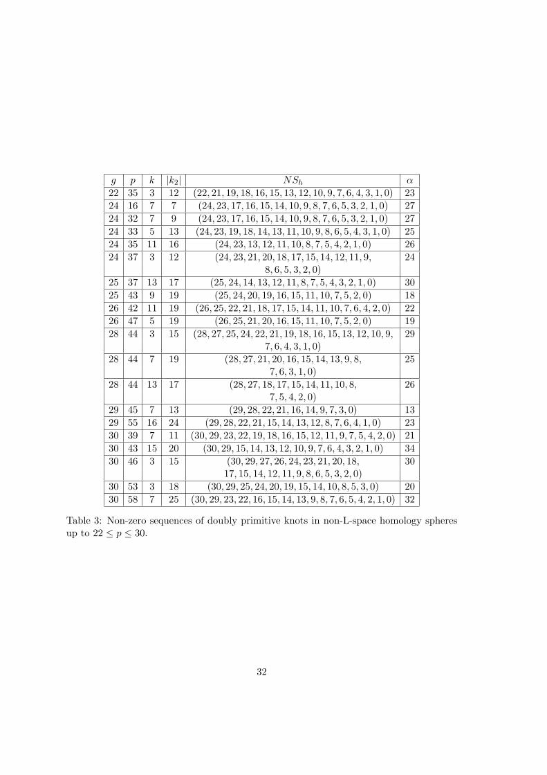
g p k |k2| NSh α

22 35 3 12 (22, 21, 19, 18, 16, 15, 13, 12, 10, 9, 7, 6, 4, 3, 1, 0) 23

24 16 7 7 (24, 23, 17, 16, 15, 14, 10, 9, 8, 7, 6, 5, 3, 2, 1, 0) 27

24 32 7 9 (24, 23, 17, 16, 15, 14, 10, 9, 8, 7, 6, 5, 3, 2, 1, 0) 27

24 33 5 13 (24, 23, 19, 18, 14, 13, 11, 10, 9, 8, 6, 5, 4, 3, 1, 0) 25

24 35 11 16 (24, 23, 13, 12, 11, 10, 8, 7, 5, 4, 2, 1, 0) 26

24 37 3 12 (24, 23, 21, 20, 18, 17, 15, 14, 12, 11, 9, 248, 6, 5, 3, 2, 0)

25 37 13 17 (25, 24, 14, 13, 12, 11, 8, 7, 5, 4, 3, 2, 1, 0) 30

25 43 9 19 (25, 24, 20, 19, 16, 15, 11, 10, 7, 5, 2, 0) 18

26 42 11 19 (26, 25, 22, 21, 18, 17, 15, 14, 11, 10, 7, 6, 4, 2, 0) 22

26 47 5 19 (26, 25, 21, 20, 16, 15, 11, 10, 7, 5, 2, 0) 19

28 44 3 15 (28, 27, 25, 24, 22, 21, 19, 18, 16, 15, 13, 12, 10, 9, 297, 6, 4, 3, 1, 0)

28 44 7 19 (28, 27, 21, 20, 16, 15, 14, 13, 9, 8, 257, 6, 3, 1, 0)

28 44 13 17 (28, 27, 18, 17, 15, 14, 11, 10, 8, 267, 5, 4, 2, 0)

29 45 7 13 (29, 28, 22, 21, 16, 14, 9, 7, 3, 0) 13

29 55 16 24 (29, 28, 22, 21, 15, 14, 13, 12, 8, 7, 6, 4, 1, 0) 23

30 39 7 11 (30, 29, 23, 22, 19, 18, 16, 15, 12, 11, 9, 7, 5, 4, 2, 0) 21

30 43 15 20 (30, 29, 15, 14, 13, 12, 10, 9, 7, 6, 4, 3, 2, 1, 0) 34

30 46 3 15 (30, 29, 27, 26, 24, 23, 21, 20, 18, 3017, 15, 14, 12, 11, 9, 8, 6, 5, 3, 2, 0)

30 53 3 18 (30, 29, 25, 24, 20, 19, 15, 14, 10, 8, 5, 3, 0) 20

30 58 7 25 (30, 29, 23, 22, 16, 15, 14, 13, 9, 8, 7, 6, 5, 4, 2, 1, 0) 32

Table 3: Non-zero sequences of doubly primitive knots in non-L-space homology spheresup to 22 ≤ p ≤ 30.

32

[9] K. Ichihara, T. Saito, and M. Teragaito, Alexander polynomials of doubly prim-itive knots, Proc. Amer. Math. Soc. 135 (2007), 605-615

[10] P. Ozsvath and Z. Szabo, On knot Floer homology and lens surgery, TopologyVolume 44, Issue 6 , November 2005, Pages 1281-1300

[11] J. Rasmussen, Lens space surgeries and L-space homology spheres ,arXiv:0710.2531

[12] M. Tange, Ozsvath-Szabo’s correction term of lens surgery, Mathematical Pro-ceedings of Cambridge Philosophical Society volume 146(2008), issue 01, pp.119-134

[13] M. Tange, On a more constraint of knots yielding lens spaces, unpublished paper(http://www.math.tsukuba.ac.jp/ tange/secondterm.pdf)

[14] M. Tange, Lens spaces given from L-space homology spheres, Experiment. Math.18 (2009), no. 3, 285-301

[15] Y. Ni, Knot Floer homology detects fibred knots, Invent. Math. 170 (2007), no.3, 577-608

Motoo TangeUniversity of Tsukuba,Ibaraki 305-8502, Japan.tange@math.tsukuba.ac.jp

33