Olsson Akesson Master 09
72
D ISTRIBUTED M OBILE C OMPUTER V ISION AND A PPLICATIONS ON THE A NDROID P LATFORM S EBASTIAN O LSSON P HILIP Å KESSON Master’s thesis 2009:E22 Faculty of Engineering Centre for Mathematical Sciences Mathematics C E T R U S C I E T I A R U A T E A T I C A R U
-
Upload
carlita-flores-araya -
Category
Documents
-
view
227 -
download
0
Transcript of Olsson Akesson Master 09

8/2/2019 Olsson Akesson Master 09
http://slidepdf.com/reader/full/olsson-akesson-master-09 1/72
DISTRIBUTEDMOBILECOMPUTER
VISION ANDAPPLICATIONS ON THEANDROIDPLATFORM
SEBASTIANOLSSONPHILIPÅKESSON
Master’s thesis2009:E22
Faculty of EngineeringCentre for Mathematical SciencesMathematics
C E NT
R UM S C I E NT I A R UMM
AT HE MAT I C A R UM

8/2/2019 Olsson Akesson Master 09
http://slidepdf.com/reader/full/olsson-akesson-master-09 2/72

8/2/2019 Olsson Akesson Master 09
http://slidepdf.com/reader/full/olsson-akesson-master-09 3/72
Abstract
This thesis describes the theory and implementation of both local and distributedsystems for object recognition on the mobile Android platform. It further describesthe possibilities and limitations of computer vision applications on modern mobiledevices. Depending on the application, some or all of the computations may be out-sourced to a server to improve performance.
The object recognition methods used are based on local features. These featuresare extracted and matched against a known set of features in the mobile device or onthe server depending on the implementation. In the thesis we describe local featuresusing the popular SIFT and SURF algorithms. The matching is done using bothsimple exhaustive search and more advanced algorithms such as kd-tree best-bin-rstsearch. To improve the quality of the matches in regards to false positives we have useddifferent RANSAC type iterative methods.
We describe two implementations of applications for single- and multi-objectrecognition, and a third, heavily optimized, SURF implementation to achieve nearreal-time tracking on the client.
The implementations are focused on the Java language and special considerationshave been taken to accommodate this. This choice of platform reects the generaldirection of the mobile industry, where an increasing amount of application develop-ment is done in high-level languages such as Java. We also investigate the use of nativeprogramming languages such as C/C++ on the same platform.
Finally, we present some possible extensions of our implementations as future work. These extensions specically take advantage of the hardware and abilities of modern mobile devices, including orientation sensors and cameras.

8/2/2019 Olsson Akesson Master 09
http://slidepdf.com/reader/full/olsson-akesson-master-09 4/72
Acknowledgments
We would like to thank our advisors Fredrik Fingal at Ep-silon IT and Carl Olsson at the Centre for MathematicalSciences at Lund University. We would further like to thank Epsilon IT for the generousaccomodations during the project.

8/2/2019 Olsson Akesson Master 09
http://slidepdf.com/reader/full/olsson-akesson-master-09 5/72
Contents
1 Introduction 3
1.1 Background . . . . . . . . . . . . . . . . . . . . . . . . . . . . . . . 31.2 Aim of the thesis . . . . . . . . . . . . . . . . . . . . . . . . . . . . 41.3 Related work . . . . . . . . . . . . . . . . . . . . . . . . . . . . . . 41.4 Overview . . . . . . . . . . . . . . . . . . . . . . . . . . . . . . . . 4
2 Theory 72.1 Object recognition . . . . . . . . . . . . . . . . . . . . . . . . . . . 72.2 Scale-Invariant Feature Transform. . . . . . . . . . . . . . . . . . . 82.3 Speeded-Up Robust Features. . . . . . . . . . . . . . . . . . . . . . 112.4 Classication . . . . . . . . . . . . . . . . . . . . . . . . . . . . . . 18
2.4.1 Overview . . . . . . . . . . . . . . . . . . . . . . . . . . . . 18
2.4.2 Nearest neighbor search . . . . . . . . . . . . . . . . . . . . 182.4.3 Optimized kd-trees . . . . . . . . . . . . . . . . . . . . . . 182.4.4 Priority queues . . . . . . . . . . . . . . . . . . . . . . . . . 192.4.5 Kd-tree nearest neighbor search. . . . . . . . . . . . . . . . 202.4.6 Best-bin-rst search . . . . . . . . . . . . . . . . . . . . . . 20
2.5 Random Sample Consensus (RANSAC). . . . . . . . . . . . . . . . 202.6 Direct linear transformation . . . . . . . . . . . . . . . . . . . . . . 22
3 Applications, implementations and case studies 273.1 Writing good mobile Android code . . . . . . . . . . . . . . . . . . 27
3.1.1 The target hardware platform . . . . . . . . . . . . . . . . . 27
3.1.2 General pointers for efcient computer vision code. . . . . . 273.1.3 Java and Android specic optimizations. . . . . . . . . . . . 29
3.2 SURF implementations. . . . . . . . . . . . . . . . . . . . . . . . . 323.2.1 JSurf . . . . . . . . . . . . . . . . . . . . . . . . . . . . . . 323.2.2 AndSurf . . . . . . . . . . . . . . . . . . . . . . . . . . . . 323.2.3 Native AndSurf (JNI, C). . . . . . . . . . . . . . . . . . . . 323.2.4 A comparison of implementations. . . . . . . . . . . . . . . 32
3.3 Applications. . . . . . . . . . . . . . . . . . . . . . . . . . . . . . . 343.3.1 Art Recognition . . . . . . . . . . . . . . . . . . . . . . . . 343.3.2 Bartendroid . . . . . . . . . . . . . . . . . . . . . . . . . . 38

8/2/2019 Olsson Akesson Master 09
http://slidepdf.com/reader/full/olsson-akesson-master-09 6/72
3.3.3 AndTracks . . . . . . . . . . . . . . . . . . . . . . . . . . . 44
4 Conclusions 514.1 Evaluation of Android as a platform for Computer Vision applications514.2 Future work . . . . . . . . . . . . . . . . . . . . . . . . . . . . . . . 51
4.2.1 Increased computational power . . . . . . . . . . . . . . . . 514.2.2 Dedicated graphical processors . . . . . . . . . . . . . . . . 524.2.3 Floating point processors . . . . . . . . . . . . . . . . . . . 524.2.4 Faster mobile access with 3G LTE. . . . . . . . . . . . . . . 52
A Android 57 A.1 Introduction . . . . . . . . . . . . . . . . . . . . . . . . . . . . . . 57
A.2 The Linux kernel . . . . . . . . . . . . . . . . . . . . . . . . . . . . 57 A.3 The system libraries. . . . . . . . . . . . . . . . . . . . . . . . . . . 59 A.4 Android runtime . . . . . . . . . . . . . . . . . . . . . . . . . . . . 59
A.4.1 Core libraries. . . . . . . . . . . . . . . . . . . . . . . . . . 59 A.4.2 Dalvik virtual machine. . . . . . . . . . . . . . . . . . . . . 59 A.4.3 The code verier. . . . . . . . . . . . . . . . . . . . . . . . 59
A.5 Application framework . . . . . . . . . . . . . . . . . . . . . . . . . 60 A.6 The structure of an application. . . . . . . . . . . . . . . . . . . . . 60
A.6.1 Activity . . . . . . . . . . . . . . . . . . . . . . . . . . . . . 60 A.6.2 Service . . . . . . . . . . . . . . . . . . . . . . . . . . . . . 60 A.6.3 Broadcast receiver. . . . . . . . . . . . . . . . . . . . . . . 61
A.6.4 Content providers . . . . . . . . . . . . . . . . . . . . . . . 61 A.7 The life cycle of an application. . . . . . . . . . . . . . . . . . . . . 61 A.7.1 Intents . . . . . . . . . . . . . . . . . . . . . . . . . . . . . 61 A.7.2 Knowing the state of an application. . . . . . . . . . . . . . 61
B Distributed computing in The Cloud 63B.1 Cloud computing services . . . . . . . . . . . . . . . . . . . . . . . 63
B.1.1 Amazon Elastic Compute Cloud (EC2). . . . . . . . . . . . 63B.1.2 Sun Grid Engine . . . . . . . . . . . . . . . . . . . . . . . . 65B.1.3 Google App Engine . . . . . . . . . . . . . . . . . . . . . . 65B.1.4 Discussion . . . . . . . . . . . . . . . . . . . . . . . . . . . 66
8/2/2019 Olsson Akesson Master 09
http://slidepdf.com/reader/full/olsson-akesson-master-09 7/72
Chapter 1
Introduction
1.1 Background
The interest in computer vision has exploded in recent years. Features such as recogni-tion and 3d construction have become available in several elds. These computationsare however advanced bothmathematically and computationally, limiting the availableend user applications.
Imaging of different sorts has become a basic feature in modern mobile phonesalong with the introduction of the camera phone, which leads to a market for com-puter vision related implementations on such platforms.
The progress in mobile application development moves more and more towardsservice development with support for multiple platforms rather than platform speciclow level development. While previous mobile development was almost exclusively done in low level languages such as assembly and C, the industry moves towards theuse of high level languages such as Java and C#. This switch is motivated by thehuge development speed up, which leads to cost decrease and feature increase and alsomotivated by the huge common code base in such languages. It is made possible by the increase in computational performance much like it was when the same type of switch was introduced on desktop computers some years ago.
Power efciency is a large issue on mobile devices, which suggests that parallel
computing with multiple cores and processor types rather than an increase in singleCPU clock speed is the way to go in mobile devices, again in the same manner as theidea of performance increase was changed in desktop computers some years ago. Theuse of dedicated processors for signaling has been utilized in mobile devices for years.Recent development has brought multiple cores and dedicated 3D graphic processorsto the mobile devices.
The move to parallel computation and the natural limits of mobile devices such asnetwork delays puts extra constraints on the high level programmer. These constraintsare normally not thought of when developing a desktop application in a high levellanguage.
3

8/2/2019 Olsson Akesson Master 09
http://slidepdf.com/reader/full/olsson-akesson-master-09 8/72
1.2 Aim of the thesis
Our goal is to study and implement computer vision applications on handheld mobiledevices, primarily based on the Android platform. We aim to do this by implementingand evaluating a number of computer vision algorithms on the Android emulator fromthe ofcial SDK, and later possibly on a real device. We also want to nd out whatkind of calculations can be practically performed on the actual mobile device and whatkind of calculations have to be performed server-side.
This master thesis will aim to use the versatility of high level development and stillperform complex computations within a time span that a user can accept.
Not all users have high speed Internet access on their mobile phones, and not allusers with high speed Internet access has unlimited data plans. Considerations have to
be taken both regarding the time it takes to send data and the actual amount of databeing transferred.
1.3 Related work
For a comprehensive look into the eld of embedded computer vision see the book Embedded computer vision[16]. This book handles specic subjects such as computa-tion with GPUs and DSPs and various real-time applications. It further discusses thechallenges of mobile computer vision.
In [13], Fritz et al SIFT descriptors are used together with an information theo-retical rejection criterion based on conditional entropy to reduce computational com-
plexity and provide robust object detection on mobile phones. We present SIFT inSection2.2 of this thesis.
An interactive museum guide is implemented by Bay et al. in [4]. This uses theSURF algorithm to recognize objects of art and is implemented on a Tablet PC. Wepresent SURF in Section2.3 of this thesis.
Ta et al. [25] implements a close to real-time version of SURF with improvedmemory usage on a Nokia N95.
Takacs et al. [26] developed a system for matching images taken with a GPS-equipped camera phone against a database of location-tagged images. They also de-vise a scheme for compressing SURF descriptors up to seven times based on entropy, without sacricing matching performance.
Wagner et al. [30] uses modied versions of SIFT and Ferns [21] for real-timepose estimation on several different mobile devices.
1.4 Overview
Chapter 2 introduces the theory behind the object recognition methods used in ourimplementations.
Chapter 3 shows some quirks with the Dalvik VM and how to circumvent themto write as efcient code as possible. We also present some of our working implemen-tations and the lessons learnt from implementing them.
4

8/2/2019 Olsson Akesson Master 09
http://slidepdf.com/reader/full/olsson-akesson-master-09 9/72
Section 3.2.1 presents our Java implementation of SURF. In Section3.2.2 we
present an Android-optimized implementation.In Section 3.3.1 we present a mobile application for recognition of paintings.
The application uses either the Scale Invariant Feature Transform (see Section2.2)or Speeded-Up Robust Features (see Section2.3) running on the handheld device todetect and extract local features. The feature descriptors are then sent to a server formatching against a database of known paintings.
In Section 3.3.2 we extend the application to recognize several objects in a singleimage. Due to the increased complexity, the feature detection and extraction is doneserver side. We also extend the matching to use best-bin-rst search (Section2.4.6)for better performance with larger databases and RANSAC (Section2.5) for increasedrobustness. We implemented a client-server application for recognizing liquor bottles
and presenting the user with drink suggestions using the available ingredients. Theserver was tested in a setup on a remote server using the Amazon Elastic ComputeCloud (EC2) to simulate a real life application setup with realistic database size.
Our third application, AndTracks, is presented in Section3.3.3. AndTracks isbased on optimized SURF and implemented in native C-code.
Finally we discuss our results and possibly future work in Chapter4. AppendixA contains a general description of the Android platform. AppendixB describes the concept of cloud computing with the biggest focus on
Amazon Elastic Cloud Compute (EC2), which is used in the Bartendroid application.
5

8/2/2019 Olsson Akesson Master 09
http://slidepdf.com/reader/full/olsson-akesson-master-09 10/72
6
8/2/2019 Olsson Akesson Master 09
http://slidepdf.com/reader/full/olsson-akesson-master-09 11/72
Chapter 2
Theory
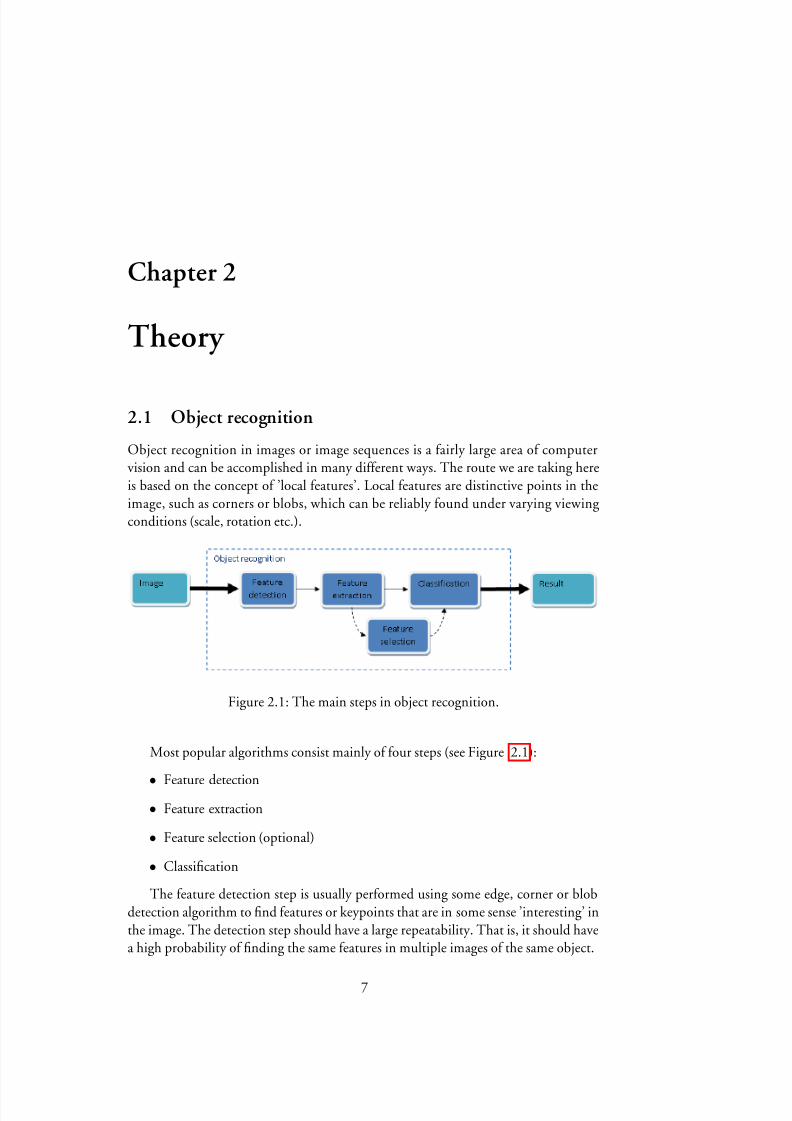
2.1 Object recognition
Object recognition in images or image sequences is a fairly large area of computervision and can be accomplished in many different ways. The route we are taking hereis based on the concept of ’local features’. Local features are distinctive points in theimage, such as corners or blobs, which can be reliably found under varying viewingconditions (scale, rotation etc.).
Figure 2.1: The main steps in object recognition.
Most popular algorithms consist mainly of four steps (see Figure2.1):
• Feature detection• Feature extraction
• Feature selection (optional)
• Classication
The feature detection step is usually performed using some edge, corner or blobdetection algorithm to nd features or keypoints that are in some sense ’interesting’ inthe image. The detection step should have a large repeatability. That is, it should havea high probability of nding the same features in multiple images of the same object.
7

8/2/2019 Olsson Akesson Master 09
http://slidepdf.com/reader/full/olsson-akesson-master-09 12/72
Feature extraction is then quantifying, or describing, the detected features so that
they can be compared and analyzed.Two of the most popular methods for feature detection and extraction are SIFT
(Section2.2) and SURF (Section2.3).The feature selection step is optional, but might include dimensionality reduction
or some information theory-based rejection criteria to make the amount of data moremanageable.
Finally, the classication step consists of comparing the extracted features to adatabase of already known features to nd the best matches. The matching can bedone for example using exhaustive nearest neighbor search (Section2.4), optimizedkd-tree search (Section2.4.5) or best-bin-rst approximate nearest neighbor search(Section2.4.6). Once the nearest neighbor search is complete, iterative methods like
RANSAC (Section2.5) can be used to discard outliers (incorrect matches) and verify the geometry to further improve the results.
2.2 Scale-Invariant Feature Transform
Overview
Scale-invariant feature transform (SIFT) is an algorithm for detection and descriptionof local image features, invariant to scale and rotation. It was introduced in 1999 by Lowe [17]. The main steps are:
1. Difference of Gaussians extrema detection
2. Keypoint localization
(a) Determine location and scale
(b) Keypoint selection based on stability measure
3. Orientation assignment
4. Keypoint descriptor
Difference of Gaussians extrema detection
The keypoints are obtained by rst creating a scale-space pyramid of differences be-tween Gaussian convolutions of the image at different scales, and then nding localextreme points.
The scale-space of an imageI ( x ; y ) is dened as the convolution function
L( x ; y ; ) a G ( x ; y ; ) £ I ( x ; y )
with the variable scale Gaussian kernel
G ( x ; y ; ) a
12
2 e ( x 2 C y 2)= 2
2:
8

8/2/2019 Olsson Akesson Master 09
http://slidepdf.com/reader/full/olsson-akesson-master-09 13/72
The result of convolving an image with the Difference of Gaussian kernel is
D( x ; y ; ) a
G ( x ; y ; k ) G ( x ; y ; )¡
£ I ( x ; y ) a L( x ; y ; k ) L( x ; y ; );
see Figure2.2.
Figure 2.2: A scale-space pyramid with increasing scale (left). Neighboring scales aresubtracted to produce the difference-of-Gaussians pyramid (right).
The difference of Gaussian is a close approximation [18] to the scale-normalizedLaplacian of Gaussian
r
2normL( x ; y ; ) a
2r
2L( x ; y ; ) a
2(L xx C L yy )
which gives strong positive response for dark blobs and strong negative response forbright blobs. This can be used to nd interest points over both space and differentscales. The relation follows from the heat diffusion equation
@ G @
a r
2G
and by nite difference approximation
r
2G ( x ; y ; ) a G xx C G yy %
G ( x ; y ; k ) G ( x ; y ; )k
so thatD( x ; y ; ) %
(k 1)
2r
2G ( x ; y ; )¡
£ I ( x ; y ):
After calculating the difference of Gaussians for each scale, each pixel is then com-pared to its 26 surrounding neighbors in the same and neighboring scales (see Fig-ure 2.3) to see if it’s a local minimum or maximum, in which case it’s considered as apossible keypoint.
9

8/2/2019 Olsson Akesson Master 09
http://slidepdf.com/reader/full/olsson-akesson-master-09 14/72
Figure 2.3: Neighboring pixels in scale-space. There are eight neighbors in the samescale and nine each in the scale above and below.
Keypoint localization step
To accurately determine a candidate keypoint’s location and scale, a 3D quadraticfunction is used to nd the interpolated maximum. The quadratic Taylor expansion with origin in the candidate point
D( x ; y ; ) a D C
@ DT
@ x x C
12 x T
@
2D@ x 2
x :
The interpolated location is found by setting the derivative of D( x ) to zero, resultingin
ˆ x a
@
2D@ x 2
1@ D
@ x :
The derivatives of D are approximated using differences between neighboring points.If the resulting locationˆ x is closer to another point, the starting position is adjustedand the interpolation repeated. The value of j D( x )j at the interpolated location is usedto reject unstable points with low contrast.
Keypoints on edges have large difference-of-Gaussian responses but poorly deter-mined location, and thus tend to be unstable. The principal curvature of an edge pointis large across the edge but small along the ridge. These curvatures can be calculatedfrom the Hessian of D evaluated at the current scale and location
H a
D xx D xy D xy D yy
!
;
The eigenvalues and of H are proportional to the principal curvatures, which arethe largest and smallest curvatures, and a large ratio between them indicates an edge.Since we only need the ratio it is sufcient to calculate
Tr( H ) a D xx C D yy a C ;
10
8/2/2019 Olsson Akesson Master 09
http://slidepdf.com/reader/full/olsson-akesson-master-09 15/72
Det( H ) a D xx D yy (D xy )2a
andTr( H )2
Det(H )a
( C )2
a
(r C )2
r 2
a
(r C 1)2
r ;
wherer is the ratio between the largest and the smallest eigenvalue ( a r ). Thresh-olding this (Lowe usedr a 10 in [18]) gives overall better stability.
Orientation assignment
When location and scale has been determined, gradient magnitude
m( x ;
y )a
q
(L( x C
1;
y ;
)
L( x
1;
y ;
))2
C
(L( x ;
y C
1;
)
L( x ;
y C
1;
))2
and orientation
( x ; y ) a tan 1
(L( x ; y C 1; ) L( x ; y C 1; ))= (L( x C 1; y ; ) L( x 1; y ; ))¡
are calculated in sample pointsaround the keypoint. The gradientsare used to build anorientation histogram with 36 bins, where each gradient is weighed by its magnitudeand a Gaussian with center in the keypoint and1: 5 times the current scale. Thehighest peaks in the histograms are used as dominant orientations and new keypointsare created for all orientations above 80% of the maximum. The orientations areaccurately determined by tting parabolas to the histogram peaks.
Keypoint descriptor
The keypoint descriptor is built by dividing the orientation-aligned region around thekeypoint into 4 ¢ 4 sub-regions with 16¢ 16 sample points and calculating 8-binhistograms of gradient orientations for each sub-region (see Figure2.4). This resultsin a 128-dimensional feature vector.
Normalization of the feature vector to unit length removes the effects of linear il-lumination changes. Some non-linear illumination invariance can also be achieved by thresholding the normalized vector to a max value of 0: 2 and then renormalizing [18].This shifts the importance from large gradient magnitudes to the general distributionof the orientations.
2.3 Speeded-Up Robust Features
Overview
Speeded-Up Robust Features (SURF) is a scale- and in-plane rotation invariant imagefeature detector and descriptor introduced in 2006 by Bay et al. SURF is comparableto SIFT in performance while being faster and more efcient to compute [3]. SURF was inspired by SIFT, and many of the steps are similar. The main steps are:
11

8/2/2019 Olsson Akesson Master 09
http://slidepdf.com/reader/full/olsson-akesson-master-09 16/72
(a)
(b)
Figure 2.4: The region around a keypoint is divided into 4¢ 4 sub-regionswith 16¢ 16sample points (a) which are then used to construct 4x4 orientation histograms with 8bins each (b).
12

8/2/2019 Olsson Akesson Master 09
http://slidepdf.com/reader/full/olsson-akesson-master-09 17/72
(a) L( x ; y ; 0) (b) L( x ; y ; )
(c) L( x ; y ; 2 )
(d) L( x ; y ; ) L( x ; y ; 0) (e) L( x ; y ; 2 ) L( x ; y ; )
Figure 2.5: Three images of Gaussians of the same source image and two imagesillustrating the difference between them
13
8/2/2019 Olsson Akesson Master 09
http://slidepdf.com/reader/full/olsson-akesson-master-09 18/72
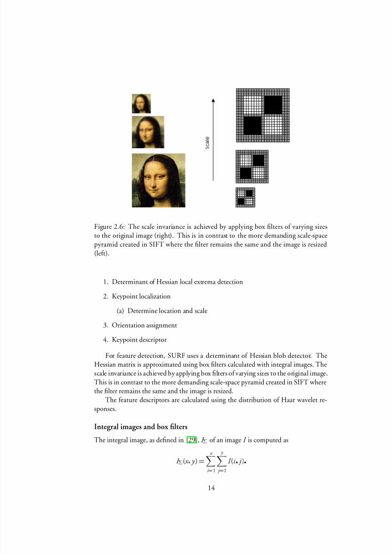
Figure 2.6: The scale invariance is achieved by applying box lters of varying sizesto the original image (right). This is in contrast to the more demanding scale-spacepyramid created in SIFT where the lter remains the same and the image is resized(left).
1. Determinant of Hessian local extrema detection
2. Keypoint localization
(a) Determine location and scale
3. Orientation assignment
4. Keypoint descriptor
For feature detection, SURF uses a determinant of Hessian blob detector. TheHessian matrix is approximated using box lters calculated with integral images. Thescale invariance is achieved by applying box lters of varying sizes to the original image.This is in contrast to the more demanding scale-space pyramid created in SIFT wherethe lter remains the same and the image is resized.
The feature descriptors are calculated using the distribution of Haar wavelet re-sponses.
Integral images and box lters
The integral image, as dened in[29], I ¦ of an imageI is computed as
I ¦ ( x ; y ) a
x
i a 1
y
j a 1
I (i ; j ):
14

8/2/2019 Olsson Akesson Master 09
http://slidepdf.com/reader/full/olsson-akesson-master-09 19/72
Σ =A-B-C+D
A B
C D
IΣ
Figure 2.7: Calculation of a rectangular area sum from an integral image.
The entry inI ¦ ( x ; y ) then contains the sum of all pixel intensities from (0; 0) to ( x ; y ),and the sum of intensities in any rectangular area inI (see Figure2.7) can be calculated with just three additions (and four memory accesses) as
x 1
x a x 0
y 1
y a y 0
I ( x ; y ) a I ¦ ( x 0 ; y 0) I ¦ ( x 1 ; y 0) I ¦ ( x 0 ; y 1) C I ¦ ( x 1 ; y 1):
This allows for fast and easy computation of convolutions with lters composed of rectangular regions, also called box lters. See for example the Haar wavelet lters inFigure2.10.
Determinant of Hessian local extrema detection
The use of the determinant of Hessian for keypoint detection can be motivated by (from Section2.2) the relation between detH and the principal curvatures, which arethe eigenvalues of H . The product a det H is called the Gaussian curvature andcan be used to nd dark/bright blobs (positive Gaussian curvature) and differentiatethem from saddle points (negative Gaussian curvature).
The scale-space Hessian matrixH ( x ; y ; ) at scale in an imageI is dened as
H ( x ; y ; ) a
L xx ( x ; y ; ) L xy ( x ; y ; )L xy ( x ; y ; ) L yy ( x ; y ; )
!
;
whereL xx , L xy and L yy are convolutions of I with the second order Gaussian deriva-tives @
2
@ x 2 g ( ), @
2
@ x @ y g ( ) and @
2
@ y 2 g ( ) respectively (see Section2.2). These second orderderivatives can be approximated efciently using integral images, with constant com-putation time as noted above. The lters and approximations used are illustrated inFigure2.8. The width of the lters used at scale is 9
1: 2 .
15

8/2/2019 Olsson Akesson Master 09
http://slidepdf.com/reader/full/olsson-akesson-master-09 20/72
(a) Discretized Gaussian second derivatives
(b) Box lter approximations
Figure 2.8: Discretized Gaussian second derivatives compared to their box lter ap-proximations. The box lters are used for calculating the determinant of Hessian inthe keypoint detection step of the SURF algorithm.
The approximate second order Gaussian derivatives are denotedL xx , L xy and L yy .From these, the determinant of the Hessian is approximated as
det (H ) % L xx L yy
w L xy
2;
where the relative weightw a 0: 9 is needed for energy conservation in the approxi-mation.
After thresholding the determinant values to only keep large enough responses,non-maximum suppression [20] is used to nd the local minima and maxima in3 ¢
3 ¢ 3 neighborhoods around each pixel in scale-space (see Figure2.3).
Keypoint localization
The candidate points are interpolated using the quadratic Taylor expansion
H ( x ; y ; ) a H ( x ) a H C
@ H T
@ x C
12 x T
@
2H @ x 2
x
16

8/2/2019 Olsson Akesson Master 09
http://slidepdf.com/reader/full/olsson-akesson-master-09 21/72
(x+6*scale,y)(x-6*scale,y)
(x,y+6*scale)
(x,y-6*scale)
(x,y)(x+6*scale,y)(x-6*scale,y)
(x,y+6*scale)
(x,y-6*scale)
(x,y)
Figure 2.9: A sliding window around the keypoint is used to nd the dominant ori-entation of Gaussian weighted Haar responses.
of the determinant of Hessian function in scale-space to determine their position withsub-pixel accuracy. The interpolation is repeated by setting the derivative
ˆ x a
@
2H @ x 2
1@ H
@ x
to zero and adjusting the position untilx is less than 0: 5 in all directions.
Orientation assignment
To nd the dominant orientation, Gaussian weighed Haar wavelet responses in the x and y directions are calculated in a circular region of radius 6 around the interestpoint. The Gaussian used for weighting is centered in the interest point and has a stan-dard deviation of 2: 5 . The Haar wavelets responses use the integral image similarly to the previously used box lters. The responses are summed in a sliding orientation window of size
3 and the longest resulting vector is the dominant orientation (seeFigure2.9).
When rotation invariance is not needed, an upright version of SURF (called U-SURF) can be computed faster since no orientation assignment is necessary. U-SURFis still robust to rotation of about¦ 15 [3].
Keypoint descriptor
The SURF descriptor is based on the distribution of rst order Haar wavelet responses(Figure 2.10), computed using integral images. When the orientation has been deter-mined, a square region of width 20 is oriented along the dominant orientation anddivided into 4 ¢ 4 sub-regions. In each sub-region Haar wavelet responses are onceagain calculated in thex and y directions at 5 ¢ 5 sample points with Haar waveletsof size 2 . The responses are then summed as
dx ,
j dx j ,
dy and
j dy j , re-sulting in four descriptor values for each sub-region and a total of 64 values for eachinterest point.
17

8/2/2019 Olsson Akesson Master 09
http://slidepdf.com/reader/full/olsson-akesson-master-09 22/72
Figure 2.10: Simple 2 rectangle Haar-like features.
2.4 Classication
2.4.1 Overview
If only a single object is to be found in an image, it is usually sufcient to match theextracted features against a database of known features, using nearest neighbor search,until a certain number of matches from the same class has been found. The classi-cation is then made by majority voting, where the image is assumed to contain theobject with most matches. If the number of objects in the image is unknown however,majority voting cannot be used and outliers need to be eliminated in another way. A common method for outlier rejection is the iterative RANSAC, which is described inSection2.5.
2.4.2 Nearest neighbor search
Given a feature descriptorq P `
d and a set of known featuresP in `
d , the nearestneighbor of q is the point p1 P P with smallest Euclidean distancej j q p1 j j (seeFigure 2.11). The featureq is assumed to belong to the same class asp1 if the ratio p1 p2
between the two closest neighbors is smaller than a threshold¢ . In [18], ¢ a 0: 8 was determined to be a good value for SIFT descriptors, eliminating 90% of the falsematches while keeping more than95% of the correct matches.
The simplest way to nd the nearest neighbors is exhaustive or naıve search, wherethe feature to be classied is directly compared to every element in the database. Thissearch is of complexity O (nd ), for n features in the database, which quickly becomesimpractical as the database grows. For large databases in high dimensions, best-bin-rst search (Section2.4.6) in optimized kd-trees (Section2.4.6) can be used instead.
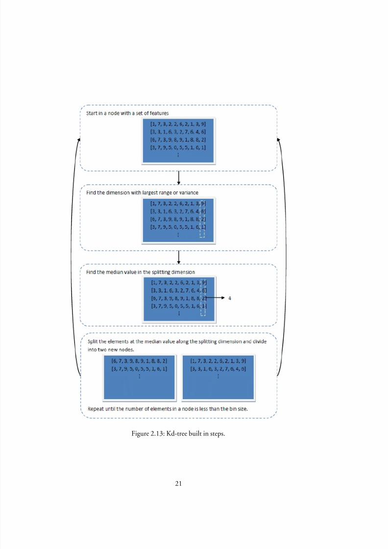
2.4.3 Optimized kd-trees
Kd-trees are k-dimensional binary trees[6], using hyperplanes to subdivide the featurespace into convex sets. See Figure2.12 for an example partition of a kd-tree in`
2.In the optimized kd-trees introduced by Friedmanet al. [12], each non-terminal
tree node contains a discriminator key (splitting dimension) and a partition value.The splitting dimension is chosen as the dimension with largest variance or range, andthe partition value as the median value in this dimension.
The tree is built recursively from a root node by deciding the splitting dimensiond , nding the median value and then placing smaller elements in the left child node
18

8/2/2019 Olsson Akesson Master 09
http://slidepdf.com/reader/full/olsson-akesson-master-09 23/72

8/2/2019 Olsson Akesson Master 09
http://slidepdf.com/reader/full/olsson-akesson-master-09 24/72
(a) (b)
Figure 2.12: A kd-tree in`
2 before (a) and after (b) partitioning.
2.4.5 Kd-tree nearest neighbor search
Exact kd-tree nearest neighbor search is only faster than naıve search up to abouttwenty dimensions[17] with practical database sizes, and as such it becomes obviousthat this does not hold for the descriptors used in SIFT or SURF. The algorithm ispresented here for reference (see Algorithm1).
A stack initially containing the root node of the kd-tree is used to keep track of which sub-trees to explore. If a child node is terminal, all elements in its bin areexamined. Examined elements are placed in a priority queue, keeping then bestmatches based on distance from the target element. If a child node is not terminal,a bounding check is performed to see if it is intersected by a hypersphere with centerin the target element and radius equal to the n:th currently best distance. If the nodepasses the bounding test, it is added to the stack and the search continues.
2.4.6 Best-bin-rst search
Best-bin-rst search was described by Beis and Lowe [5] as an approximate nearestneighbor search based on optimized kd-trees. It uses a priority queue instead of astack to search branches in order of ascending distance from the target point andreturn the m nearest neighbors with high probability, see Algorithm2. The searchis halted after a certain numbern
binsof bins have been explored, and an approximate
answer is returned. According to[18], a cut-off after 200 searched bins in a database of 100; 000 keypoints provides a speedup over the exact search by 2 orders of magnitude, while maintaining95% of the precision.
2.5 Random Sample Consensus (RANSAC)
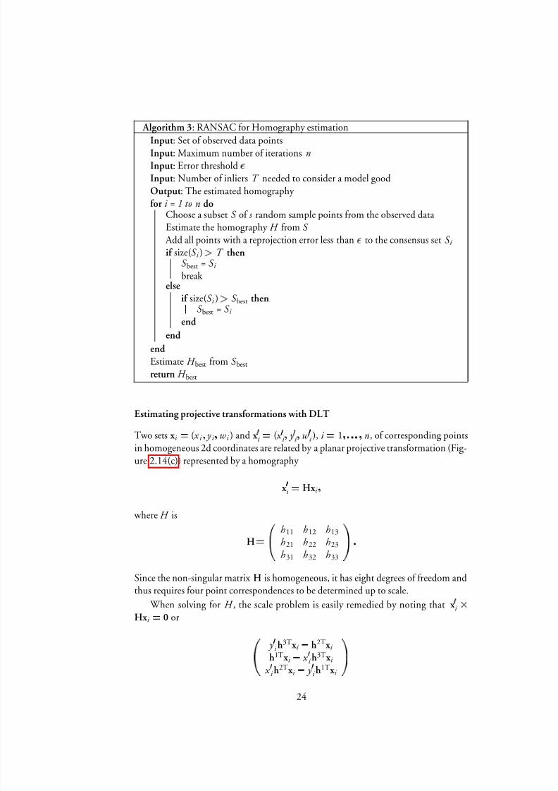
RANSAC is an iterative method (see Algorithm3) for estimating model parametersto observed data with outliers.
When using RANSAC to remove outliers from matching image points, a homog-
20
8/2/2019 Olsson Akesson Master 09
http://slidepdf.com/reader/full/olsson-akesson-master-09 25/72
Figure 2.13: Kd-tree built in steps.
21

8/2/2019 Olsson Akesson Master 09
http://slidepdf.com/reader/full/olsson-akesson-master-09 26/72
Algorithm 1: Kd-tree n-nearest neighbor algorithmInput : Query elementq Input : Root node of an optimized kd-treeOutput : Priority queueR containing the n nearest neighborsS = stack for nodes to explorePut the root node on top of S whileS is not empty do
Pop the current node fromS foreach Child node C of the current node do
if C is a leaf node thenExamine all elements in the bin and insert intoR
else
r = the n:th currently best distance in the priority queueif C is intersected by a hypersphere of radius r around q then AddC to S
endend
endendreturn R
raphy matrixH relating the matches as
x H
a Hx
is used as a model. The homography can be estimated using the Direct Linear Trans-formation (Section2.6). The error measurement used in the algorithm is the repro- jection error j j x H
Hx j j 2.RANSAC works by randomly selecting a subset of the matching image points and
estimating a homography to it. All points tting the model with an error less than acertain threshold are determined to be inliers and placed in a consensus set.
If the number of points in the consensus set is above the number of inliers neededfor the model to be considered good, the homography is re-estimated from all inliersand the algorithm terminated. If not, a new random subset is chosen and a new homography estimated.
When the maximum number of iterations has been reached, the homography isre-estimated from the largest consensus set and returned.
2.6 Direct linear transformation
The Direct Linear Transformation (DLT) can be used to nd a homography H be-tween 2D point correspondencesx i and x H
i in homogeneous coordinates [11].
22

8/2/2019 Olsson Akesson Master 09
http://slidepdf.com/reader/full/olsson-akesson-master-09 27/72
Algorithm 2: Best-bin-rstn-nearest neighbor searchInput : Query element
q Input : Root node of an optimized kd-treeOutput : Priority queueR containing the n nearest neighborsS = priority queue for nodes to explorePut the root node in S while S is not empty do
Pop the current node fromS foreach Child node C of the current node do
if C is a leaf node thenExamine all elements in the bin and insert intoR if nbins bins have been explored then
return R end
elser = the n:th currently best distance in the priority queueif C is intersected by a hypersphere of radius r around q then
AddC to S end
endend
endreturn R
23
8/2/2019 Olsson Akesson Master 09
http://slidepdf.com/reader/full/olsson-akesson-master-09 28/72
Algorithm 3: RANSAC for Homography estimationInput : Set of observed data pointsInput : Maximum number of iterationsnInput : Error threshold
Input : Number of inliersT needed to consider a model goodOutput : The estimated homography for i = 1 ton do
Choose a subsetS of s random sample points from the observed dataEstimate the homography H from S Add all points with a reprojection error less than to the consensus setS i if size(S i ) > T then
S best = S i
break elseif size(S i ) > S best then
S best = S i end
endendEstimate H best from S bestreturn H best
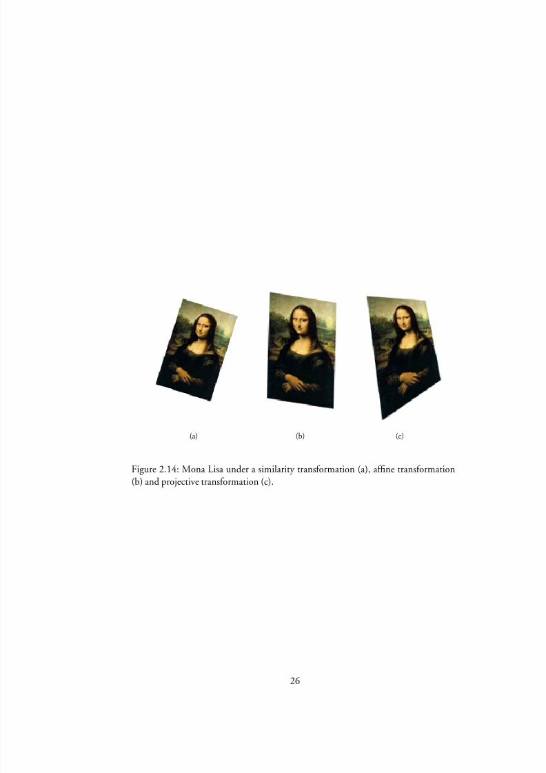
Estimating projective transformations with DLTTwo setsx i a ( x i ; y i ; w i ) and x H
i a ( x H
i ; y H
i ; w H
i ), i a 1; : : : ; n, of corresponding pointsin homogeneous 2d coordinates are related by a planar projective transformation (Fig-ure 2.14(c)) represented by a homography
x H
i a Hx i ;
whereH is
H a
H
d
h11 h12 h13h21 h22 h23
h31 h32 h33
I
e
:
Since the non-singular matrixH is homogeneous, it has eight degrees of freedom andthus requires four point correspondences to be determined up to scale.
When solving forH , the scale problem is easily remedied by noting thatx H
i ¢
Hx i a 0 or
H
d
y H
i h3T x i h2T x i
h1T x i x H
i h3T x i
x H
i h2T x i y H
i h1T x i
I
e
24

8/2/2019 Olsson Akesson Master 09
http://slidepdf.com/reader/full/olsson-akesson-master-09 29/72
whereh j Ta (h j 1 ; h j 2 ; h j 3). This can be rewritten as
P
R
0T x Ti y H
i x Ti x Ti 0T
x H
i x Ti y H
i x Ti x H
i x Ti 0T
Q
S
H
d
h1
h2
h3
I
e
a A i h a 0
which is a set of linear equations inh that can be solved using standard methods. Since we generally do not have exact point correspondences, an approximate solution canbe found using for example Singular Value Decomposition [15],
A a USV T :
The solution h is the the singular vector corresponding to the smallest singular value.If the singular values inS are sorted in descending order, this is the last column of V .The resulting homography H is then given fromh.
To get robust estimation, all points should be normalized before estimatingH[15]. The normalization is performed separately forx i and x H
i by centering the pointsaround the origin and scaling their mean distance from origin to
p
2.If ˆ x i a T x and ˆ x H
i a T H x H are the normalized points andH is the homography from ˆ x to x H , then H a T H 1HT is the homography fromx to x H .
Afne and similarity transformations
An afne transformation maps parallel lines to parallel lines, but orthogonality is not
preserved (as illustrated in Figure2.14(b)). A two-dimensional afne transformationcan be expressed as
H a
H
d
h11 h12 t x h21 h22 t y 0 0 1
I
e
;
wheret x and t y is the translation. Estimation of the afne transformation is done inthe same way as above, requiring three point correspondences since it has six degreesof freedom.
When only two matching points are available, it is still possible to estimate thetranslation t x and t y , rotation and scales with a similarity transformation (see Fig-ure 2.14(a))
H
d
s cos s sin t x
s sin s cos t y 0 0 1
I
e
:
The similarity transformation has four degrees of freedom and can thus be estimatedfrom only two point correspondences.
25
8/2/2019 Olsson Akesson Master 09
http://slidepdf.com/reader/full/olsson-akesson-master-09 30/72
(a) (b) (c)
Figure 2.14: Mona Lisa under a similarity transformation (a), afne transformation(b) and projective transformation (c).
26

8/2/2019 Olsson Akesson Master 09
http://slidepdf.com/reader/full/olsson-akesson-master-09 31/72
Chapter 3
Applications, implementations and
case studies3.1 Writing good mobile Android code
3.1.1 The target hardware platform
The implementations of this thesis have been targeted at the Android Dev Phone 1.This is essentially an HTC Dream (G1) phone without operator locks. The relevanthardware specications are:
• Qualcomm MSM7201A ARM11 processor at 528MHz
• 3.2 inch capacitive touch screen
• 192 MB DDR SDRAM and 256 MB Flash memory
• 3.2 megapixel camera with auto focus
• Quad band mobile network access and 802.11 b/g wireless LAN connectivity
3.1.2 General pointers for efcient computer vision code
Introduction
Handling images involves large matrices and complex algorithms.One must understand the nature of the target platform in order to understand
how to write efcient code. Incorrect handling of memory and oating point valuescan make a computer vision implementation run many times slower than it could do with rather simple code changes.
However, it should be noted that micro optimizations should not be used insteadof algorithmic optimizations, but rather as a complement.
A general overview of the Android platform can be found in AppendixA .
27

8/2/2019 Olsson Akesson Master 09
http://slidepdf.com/reader/full/olsson-akesson-master-09 32/72
Handling matrices
Image handling is essentially handling large matrices and the implementations in thisthesis are no exceptions. The Java collections package is very useful, but carries toomuch overhead in comparison to speed when it comes to computer vision. This isespecially evident in mobile implementations. Using basic arrays is almost alwayspreferred for the heavy algorithms. There are pitfalls even with arrays as data storage. Java can handle multi dimensional matrices with the syntaxarray[m pos][n pos] ,but accessing these matrices is much slower than accessing a one dimensional array such asarray[pos] . It is for this reason better to address two dimensional matricesthrough one single dimension of sizewidth £ height by addressing asarray[ row £
width C col ] . This abovementioned layout of the array can and should of coursebe changed to t the order in which memory is accessed. It is much faster to accesselements in orderarray[pos], array[pos+1], array[pos+2] than for exam-ple array[0], array[1000], array[2000] . This might not seem completely obvious due to the O (1) nature of array access, but the access will be optimized by the caching functions of the processor and virtual machine and the next element willtherefore often be available to the application even before a request has been sent to thememory pipeline. Accessing the array out of order will render constant cache misses which will lead to delays due to the slow nature of RAM in comparison to cache.
Floating point operations
Computer vision implementations are most often heavily based on oating point val-
ues since most operations cannot be realized by integer numbers. Handling oatingpoint values on a desktop computer is often as fast as integer numbers due to hard- ware implementations for fast oating point operators. Embedded devices such asmobile phones will however most often not include oating point compatible proces-sors. Floating point operations will be implemented in software in such applications,rendering the operations many times slower than said operations using integers.
The magnitude of this obstacle can however be lowered by good programmingpractices. As with all mobile development one has to take limitations in to consider-ations continuously, and one way is to always use integers when possible. Programscan often contain thousands of unnecessary oating point operations on integer num-bers or even countable numbers in decimal form. An obvious remedy is to realizecountables such as 0: 1; 0: 2; 0: 3 as 1; 2; 3 .
If remedies cannot be found as easily as mentioned above one should considerusing xed point arithmethic. Specifying the position of the decimal point can oftenbe done for a specic computer vision application, but limits of the input to saidfunction must be implemented due to the risk of unwanted behavior in any realm where the xed point operations give too inaccurate answers. Fixed point numberscan in many situations give more precise answers than oating point operations dueto the inexact nature of oating point numbers, but if the xed decimal point positionis not carefully chosen to match the number of signicant gures the results can leadto overows and other unwanted behavior.
28

8/2/2019 Olsson Akesson Master 09
http://slidepdf.com/reader/full/olsson-akesson-master-09 33/72
This leads to the conclusion that one should be aware and replace unnecessary
oating point values and implement xed point operations where speed is an issue.
3.1.3 Java and Android specic optimizations
Introduction
Since Android provides the possibility to implement Java code with standard industry methodologies, it is of course possible and sometimes preferable to use the same struc-ture of implementation as one would on a normal desktop application. The targetsystems will however have the same hardware limitations as any other mobile platformdoes. This means that some measures have to be taken in order to produce code thatcan run smoothly. This problem is very evident when it comes to processes with high
computational complexity such as object recognition.The Android platform is built with a high priority on the keeping of a small
memory footprint rather than keeping the processing speed up. This means that somecommon usages such as method nestling on the stack and context switching betweendifferent threads are implemented in a way that preserves memory rather than pro-cesses quickly [2].
Using static references when possible
Since the creation of objects and the keeping of said objects in memory are costly onthe Android platform, the use of static methods where possible is recommended. Thisis of course in contrary to common Java methodology which means the developer hasto compare the possible scenarios and use the most tting method.
One has to remember that Java does not have explicit freeing of the memory. Thisis handled by a garbage collector which looks for unused objects and frees the memory they used when it is sure that this object cannot be used again. Static references cansometimes be useful on the Android platform in order to make sure that unused datais not kept in memory even though other parts of the same object is to be used later.The garbage collector will not be able to run smoothly in parallel if a lot of unuseddata is kept for a long time and later freed all together at the same time.
Referencing objects wisely
This section is connected to the previous section since it also concerns the garbagecollector. The garbage collector will not be able to free large objects that are still usedin parts. Keeping unnecessarily large object is a common error in Android graphicsdevelopment. One will often nd oneself in situations where the ”context” of thecurrent activity has to be sent to a method that displays graphics. It will often bepossible to send objects that are in a high level of the application and get the expectedbehavior, but this also means that said level cannot be freed by the garbage collectoruntil the method is done. If one sends the lowest possible object level to the samegraphics method there will be a greater possibility that most of the memory can befreed. An example can be seen in Listing3.1. In this listing one can see that if the
29

8/2/2019 Olsson Akesson Master 09
http://slidepdf.com/reader/full/olsson-akesson-master-09 34/72
high level object is passed on to gain access to the view, one will have to keep the
useless objects until the high level object is released by the method it is passed on to.Referencing the low level object instead will make it possible to free the high levelobject. This problem can often be passed on in further calls, making the high levelobject live long past its recommended expiration time.
Listing 3.1: An example of object referencing< High level object that is referenced instead of low level object>
< Useless objects ought to be collected by the garbage collector>
< Low level object which ought to be referenced instead of the high level object>
< Useful view that the receiving method wants to gain access to>
Listing 3.2: Some loop examples/∗Example 1 shows a bad looping practice since the length of ”vec” will be referenced run and the addition of 2 will also be done each time.∗/for (int i = 0; i< vec.length+2; i++){
//Do something}
/∗Example 2 shows how example 1 can be improved to run faster due to lesscalls to the eld length and less additions.∗/int maxI = vec.length+2;for (int i = 0; i< maxI; i++){
//Do something
}/∗Example 3 shows a bad looping practice for iteration over a Javacollections object. Calling hasNext() and next() on the iterator each time will be very costly.∗/Iterator< String> myIterator = myCollection.iterator(); while (myIterator.hasNext()){
String myString = myIterator.next();//Do something with myString
}
/∗Usage of the ”for each” loop will most often make a local reference of the objectsin array form and thus keep the number of method calls at a minimum.∗/for (String myString: myCollection){
//Do something with myString}
Looping wisely
The Dalvik compiler and verier contains very few optimizations that most normal JREs do, which makes wise looping a high priority. This has lead to behavior such asthe fact that the iterator concept is very slow on Android and should never be used.Manual caching of values such as loop stop values is recommended as well as the use
30

8/2/2019 Olsson Akesson Master 09
http://slidepdf.com/reader/full/olsson-akesson-master-09 35/72
of the Java 1.5 ”for each” loop in the cases where the underlying implementation is
free of time consuming procedures such as iterators. Listing3.2 shows some examplesof how large structures should and should not be iterated over.
If one needs to loop the same amount of times over multiple collections it isrecommended to rst retrieve the collection data as a local array with toArray() andretrieve data from these arrays instead. This will add the overhead of the new array,but since it will only contain references to objects it will take very little memory andthe advantage of the speed up will be worth it.
Using native C/C++ through JNI for high performance methods
Although Android programs are written in Java it is possible to cross compile hard- ware specic code and utilize in Java using the Java Native Interface (JNI). In someimplementations this will give a high performance boost. This could be especially interesting in computer vision applications.
There are some important points that one should know prior to JNI implementa-tion:
• One must recognize the fact that the use of JNI somewhat defeats the purposeof Android’s Java concept since the implementations will be at least processorarchitecture specic, and at most processor specic. This will however not be abig problem in many cases since the JNI code will most often be smaller code
snippets that perform large loops. The code will most often be compilable onmost platforms and such advanced solutions will probably often be bundled with hardware or at least specic for said hardware.
• Due to the fact that it is preferable not to use Java collections and similar in Android it is often simple to convert existing Java code to C code without muchhassle. This code will of course not be optimized for C, but on the other handit will still often be much faster than the equivalent Java implementation.
• A very important thing to remember is that if one is to optimize large loops with JNI one should include the loop in JNI and not just the calculations within.
The large cost of the repeated context switches in Android will otherwise inmany cases be higher than just running everything in Java.
• One must make sure that the native code is extremely stable. It must be testedfor all possible input types. If the native code crashes it will destabilize the wholeVM (Dalvik) and will most likely cause your application to crash without thepossibility to display a message. This means that if the native code leads to asegmentation fault due to a bad memory pointer it will terminate the wholeapplication. One must thus remember to check the input data in Java beforethe JNI call, because there is no exception handling to rely on.
31

8/2/2019 Olsson Akesson Master 09
http://slidepdf.com/reader/full/olsson-akesson-master-09 36/72
3.2 SURF implementations
3.2.1 JSurf
JSurf is our Java implementation of SURF. JSurf was originally a port of OpenSURF1.2.1. We have since rewritten the whole library to implement our own optimizationsspecic for Java, instead of following the development of OpenSURF. Our aim is torelease it as open source.
3.2.2 AndSurf
AndSurf is an Android optimized version of JSurf. AndSurf is tted to overcomethe algorithmic aws and choices of the Android platform. This includes inliningof methods to reduce context switches and removal of all Java collections and otherimports in favor to primitive types such as integer arrays and oat arrays.
3.2.3 Native AndSurf (JNI, C)
AndSurf was very slightly modied to become C code instead of Java and includedthrough the JNI interface. This proved slightly faster than the Java implementationon a desktop computer and many times faster than the Java implementation on themobile phone. This proves that native code still is important for slightly heavy com-putations on mobile devices. One should however still do most of the application in Java and use the native code to overcome certain obstacles when needed.
3.2.4 A comparison of implementations
To benchmark our SURF implementations we chose to compare our implementationsto each other and to certain known implementations. All benchmarks are done withSURF upright descriptors.
In the desktop case we chose to compare AndSurf, JSurf, AndSurf in native code,OpenSURF, OpenCV’s implementation of SURF and the original SURF implemen-
tation (available in binary format). This can be seen in Figure3.1. All native im-plementations used comparable compiler optimizations. It is interesting to noticethat C implementation outranks all the other implementations and that our Java im-plementations are comparable for small images and as fast or faster than known Cimplementations on larger images.
In the mobile case we chose to compare AndSurf, JSurf and our AndSurf JNIimplementations. This can be seen in Figure3.2. The tests were done on the An-droid Developer Phone 1 (ADP1), which is essentially a HTC G1 (”Dream”). It isnotable that the native implementation is approximately ten times faster than the Javaimplementations on the mobile phone, while on the desktop it is only 2-3 times faster.
32

8/2/2019 Olsson Akesson Master 09
http://slidepdf.com/reader/full/olsson-akesson-master-09 37/72
Figure 3.1: The average count of millisecond per discovered feature with comparablesettings for different SURF implementations on a desktop computer.
Figure 3.2: The average count of milliseconds per discovered feature with comparablesettings for different SURF implementations on the Android Developer Phone 1, orHTC G1 (”Dream”).
33

8/2/2019 Olsson Akesson Master 09
http://slidepdf.com/reader/full/olsson-akesson-master-09 38/72
3.3 Applications3.3.1 Art Recognition
Purpose
The purpose of this application is to be able to identify paintings via the camera of themobile phone. After identication the user should be presented with additional infor-mation regarding the painting and the painter. One should be able to read about otherpaintings by said painter and an additional function could be to receive suggestionson similar art.
Basic structure
The application is implemented as a client-server set-up. The client takes a pictureof a painting and extracts local features, which are sent to the server. The server willcompare these features against a database of known paintings and their local features.The server will then send formatted results with the relevant information regardingthis painting.
Taking a picture
As can be seen in Figure3.3(a) a picture is taken using the camera of the mobile phone.This picture is then resized to a smaller size if it is unnecessarily large.
Extracting features and recognizing art
This is the heart of the application and can be seen in Figure3.3(b). Instead of sendingthe picture to the server for feature extraction, the process is done on the phone. Thephone will extract one feature at a time and immediately send it to the server, whichperforms recognition as soon as a feature is available.
Even though extraction is slower on the client than it would be on a server, it willallow for plenty more clients per server. As an added bonus the local features will bemarked in the picture in a cognitively rewarding fashion as opposed to just waiting forthe delays of the network and the server’s feature extraction to be done.
34

8/2/2019 Olsson Akesson Master 09
http://slidepdf.com/reader/full/olsson-akesson-master-09 39/72
(a) Taking a picture to recognize (b) Features are extracted and sent to theserver
(c) The calculated boundaries of the objectare cut
(d) The results and suggested informationis displayed
Figure 3.3: A picture of a painting is recognized with the phone.
35
8/2/2019 Olsson Akesson Master 09
http://slidepdf.com/reader/full/olsson-akesson-master-09 40/72
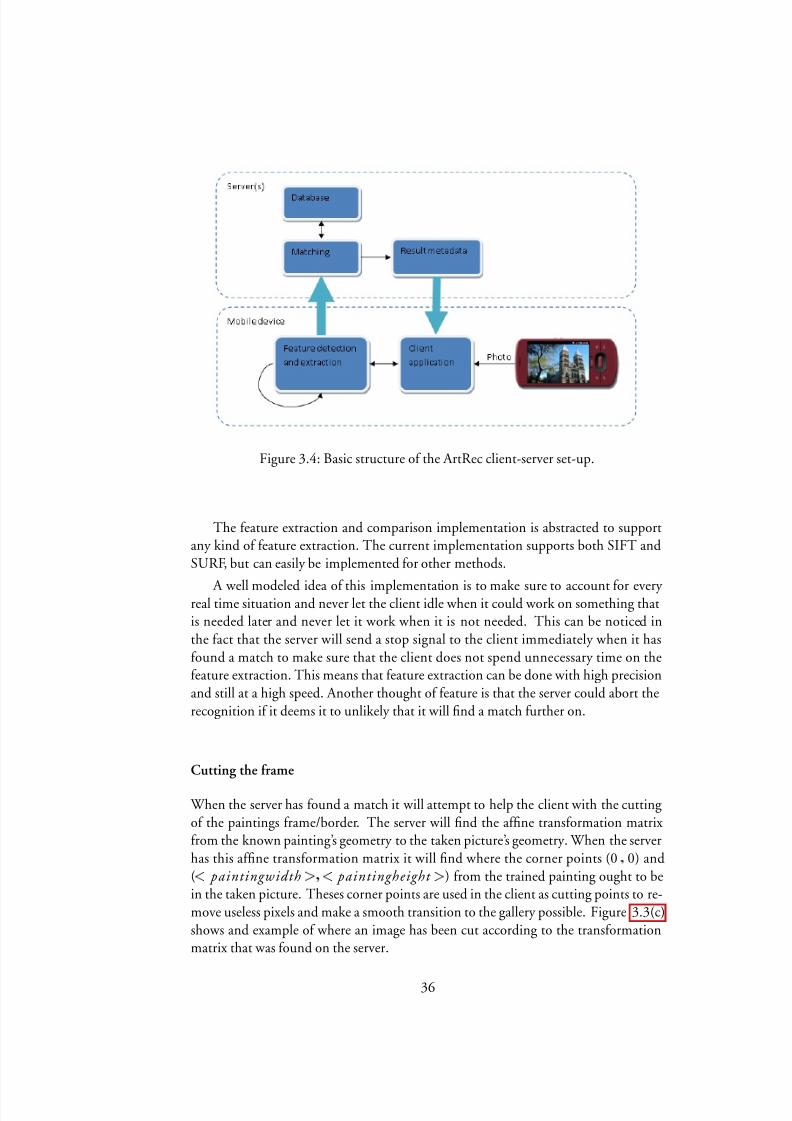
Figure 3.4: Basic structure of the ArtRec client-server set-up.
The feature extraction and comparison implementation is abstracted to supportany kind of feature extraction. The current implementation supports both SIFT andSURF, but can easily be implemented for other methods.
A well modeled idea of this implementation is to make sure to account for every real time situation and never let the client idle when it could work on something thatis needed later and never let it work when it is not needed. This can be noticed inthe fact that the server will send a stop signal to the client immediately when it hasfound a match to make sure that the client does not spend unnecessary time on thefeature extraction. This means that feature extraction can be done with high precisionand still at a high speed. Another thought of feature is that the server could abort therecognition if it deems it to unlikely that it will nd a match further on.
Cutting the frame
When the server has found a match it will attempt to help the client with the cuttingof the paintings frame/border. The server will nd the afne transformation matrixfrom the known painting’s geometry to the taken picture’s geometry. When the serverhas this afne transformation matrix it will nd where the corner points (0; 0) and(< paintingwidth > ; < paintingheight > ) from the trained painting ought to bein the taken picture. Theses corner points are used in the client as cutting points to re-move useless pixels and make a smooth transition to the gallery possible. Figure3.3(c)shows and example of where an image has been cut according to the transformationmatrix that was found on the server.
36

8/2/2019 Olsson Akesson Master 09
http://slidepdf.com/reader/full/olsson-akesson-master-09 41/72
Displaying the gallery
If a result is found the application will translate and resize the cut picture with ananimation that fades into the correct gallery position. The gallery can be seen inFigure3.3(d) and it displays information about the recognized painting and also aboutother paintings by this painter.
An example session
The user will select which method it prefers and send the command using a protocolas below:
beginRecognition SURF clientside
<local feature><local feature>...<local feature>endRecognition
The above example assumes that all local features have to be sent. In a normalcase where a match has been found prematurely it will break when possible (prior toendRecognition ).
In the case where the server has found a match it will send an answer as below:
beginRecResponse2,10,100,12leonardo_da_vinci.mona_lisa.jpgendRecResponse
Where 2,10,100,12 are the cutting points ( x 0, y 0, x 1, y 1) andleonardo_da_vinci.mona_lisa.jpg tells the client where to look for painterinformation and which painting of the painter one has photographed. The paint-ing information is gathered from a web server with known directory syntax for fastfetching and formatting using XML and HTML.
There is support for both setting which local feature extraction method to use and
also sending settings to said method as can be seen in the above examples where SURFis the method and no settings are sent (blank line).
Evaluation
We began by modifying an available SIFT implementation to t our needs. Thisincluded some optimizations and behavior modications to be able to interact withour thought out program structure. Extracting feature from an image on the phoneusing SIFT proved very time consuming even with our optimizations.
Our next step was to look for an available Java implementation of the SURF al-gorithm, which is faster than SIFT in most cases. Since no satisfying implementation
37

8/2/2019 Olsson Akesson Master 09
http://slidepdf.com/reader/full/olsson-akesson-master-09 42/72
was available, we implemented SURF in Java as mentioned in Section3.2.1. We no-
ticed that the preparation of the determinant of Hessian matrix took a large portionof the application time even though only parts of the matrix were needed if sufcientinformation was found in a painting. Since experienced speed was a large issue, weopted to ll portions of the determinant matrix when needed in the extraction process.The extraction process continuously sends features to the server, which performs com-parisons to known features immediately. When sufcient information is available tothe server, it will tell the client to stop extraction which leads to very few unnecessary computations, including determinant of Hessian computations.
It was noticed that the amount of false positives quickly grew as the database grew due to the simple hard limit for the number of feature matches. We realized thatsome kind of geometric comparison method such as RANSAC was needed to discard
outliers and provide better answers in a database with more than a few pictures. Yet another crucial problem was quickly noticed. It quickly became obvious that
the search time on the server grew rapidly as the database increased. This showed thata simple exhaustive search using an Euclidean distance metric is too slow for a usefulapplication with hundreds of pictures in the database. The search time for such adatabase can be seen in Figure3.6(a).
3.3.2 Bartendroid
Purpose
The purpose of this application is to beable to identify multiple bottles in a pic-ture and use that information in order toinform the user of possible drink combi-nations which can be mixed from saidingredient. After the recognition andsuggestion nding is done the user ispresented with a list of possible drinksand the ability to read the recipes andlearn more about the beverages.
Limitations
This application requires much morefeature extraction and also requires thepossibility to lter the features more ef-ciently than the art recognition did. Thisis due to the fact that the input im-age will be able to have multiple objectmatching to different known object and that these individual object can be situatedanywhere in the image. Art recognition will most often handle an input image thatmainly consists of the painting and has very little noise. Since the art recognition
38

8/2/2019 Olsson Akesson Master 09
http://slidepdf.com/reader/full/olsson-akesson-master-09 43/72
was dependent on the ability to stop nding features when the recognition was good
enough and this implementation will have to continue searching for features until theextraction process is done it will not be plausible to do the feature extraction on theclient side.
Basic structure
The basic structure of the Bartendroid client-server setup can be seen in Figure3.5.The client snaps a picture of a collection of beverages, which is sent to the server
for recognition. This means that the option to extract features locally is not availablefor reasons mentioned previously. The server will reply with identication names forthe beverages and the client can ask the server for recipes using said beverages if it isinterested.
Extracting features and recognizing beverages
The server will receive an image in binary form and perform some kind of featureextraction on the image. These extracted features will be matched against a known setof features to nd tting match pairs. Since the amount of features required to be ableto recognize many different sorts of beverages from somewhat different angles is very large, a naıve approach is not feasible. The implementation instead utilizes a kd-treeof known features and does a tree search for approximate matches with an acceptableerror probability.
The search algorithm works by rst nding all matching features in the feature
database. These matches are sorted by which destination image in the database they match so that the located bottles can be separated from each other. If the amount of matches to a database image is high enough, which is approximately 10 good matchesin our implementation, the matches are passed on to the next step.
Since the database must be able to contain hundreds of bottles there will oftenbe incorrect matches that survive the initial thresholding. This means that a simplethreshold for match count is not a good enough parameter for identication and fur-ther steps need to be taken to remove the outliers. RANSAC is used for each matchingfeature set to lter out the geometrically impossible matches such as mirrored pointmatches. Once again this will be approximate and not always give an answer, but withthe appropriate amount of tries it will give an acceptable error rate. The matches thatsurvived RANSAC is considered correct and the identication strings of the matchingobjects are sent to the client.
When testing Bartendroid we chose to place it on a Amazon Elastic ComputeCloud (EC2) server to imitate a real world application setup of varying database sizes.For more information on EC2 see AppendixB.1.1. This server was run on the EC2”High-CPU Medium Instance” with Ubuntu Linux. The server trained on differentimage set sizes and a kd-tree was built ofine for fast searching when a request wouldcome in. We began by using a simple exhaustive feature to feature Euclidean distance-match method like the server side of Art Recognition had used. This proved very slow as the database size increased and without RANSAC the results become less and less
39

8/2/2019 Olsson Akesson Master 09
http://slidepdf.com/reader/full/olsson-akesson-master-09 44/72
Figure 3.5: Basic structure of the Bartendroid client-server set-up.
reliable. In Figure3.6(a) one can see the time needed for searching different databasesizes on the EC2. As can be seen it scales very poorly since the search time is increasedlinearly as the amount of features is increased.
With these results in mind we turned to a best-bin-rst kd-tree implementation(See Section2.4.6) together with RANSAC for more useful and faster results. This would prove to be much faster and robust to different database sizes and image types.The end to end time from the photo being taken to the results being presented was ap-proximately 10 seconds with most database cases on a wireless LAN network connec-tion and it took approximately twice that time when sending pictures on a UMTS mo-bile connection. The interesting part is the combined time for search and RANSACas the database is increased with large amounts of features from other objects than thesought after ones. In Figure3.6(b) it can be seen that the search time seems to beincreased logarithmically as the number of features is increased, which is seen as a lineon the logarithmic scale. It should further be noted that the computation time seemsto be approximately 2 seconds with a database of one million features. One millionfeatures would approximately be the amount needed to describe one thousand bot-tles. This implementation mostly uses one processor core of the two available, whichmeans that two concurrent Bartendroid sessions could be running on the EC2 withthe same separate speed as Figure3.6(b) shows.
Requesting drink suggestions
The client will receive the list of matching beverages. The client can choose to requestdrink matches for these beverages, a subset of the beverages or even other beverages.
40

8/2/2019 Olsson Akesson Master 09
http://slidepdf.com/reader/full/olsson-akesson-master-09 45/72
0 0.5 1 1.5 2 2.5
x 105
0
0.5
1
1.5
2
2.5
3
3.5
4x 10
4
Number of features in database
T i m e
( m s
)
(a) The exhaustive search time as the feature database is increased
10 3 10 4 10 5 10 6 10 7
600
800
1000
1200
1400
1600
1800
2000
2200
2400
Number of features in database
T i m e
( m s
)
(b) The best-bin-rst kd-tree search and RANSAC time as the feature database is in-creased. Notice the logarithmic scale on the size axis.
Figure 3.6: The search time for the available methods of the ArtRecognition andBartendroid server. An image will at an average consist of approximately 500 features. A bottle will be described by between one and four images in Bartendroid.
41
8/2/2019 Olsson Akesson Master 09
http://slidepdf.com/reader/full/olsson-akesson-master-09 46/72
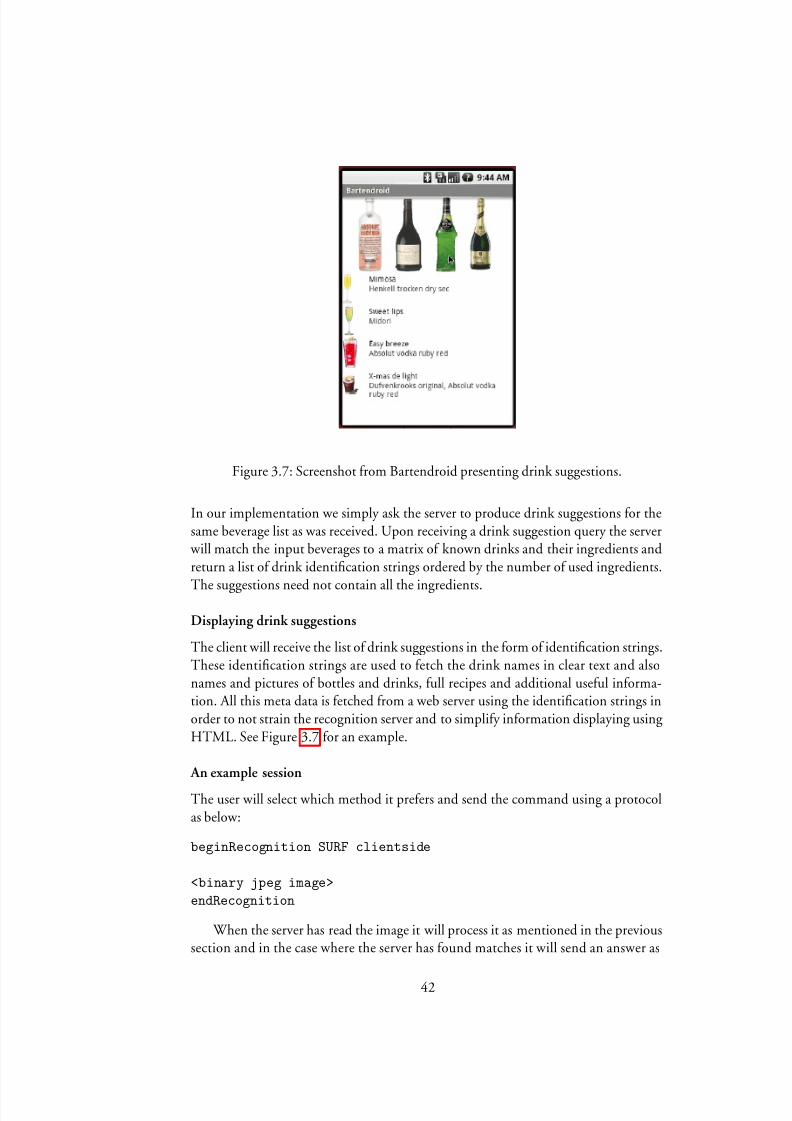
Figure 3.7: Screenshot from Bartendroid presenting drink suggestions.
In our implementation we simply ask the server to produce drink suggestions for thesame beverage list as was received. Upon receiving a drink suggestion query the server will match the input beverages to a matrix of known drinks and their ingredients andreturn a list of drink identication strings ordered by the number of used ingredients.
The suggestions need not contain all the ingredients.
Displaying drink suggestions
The client will receive the list of drink suggestions in the form of identication strings.These identication strings are used to fetch the drink names in clear text and alsonames and pictures of bottles and drinks, full recipes and additional useful informa-tion. All this meta data is fetched from a web server using the identication strings inorder to not strain the recognition server and to simplify information displaying usingHTML. See Figure3.7 for an example.
An example session
The user will select which method it prefers and send the command using a protocolas below:
beginRecognition SURF clientside
<binary jpeg image>endRecognition
When the server has read the image it will process it as mentioned in the previoussection and in the case where the server has found matches it will send an answer as
42

8/2/2019 Olsson Akesson Master 09
http://slidepdf.com/reader/full/olsson-akesson-master-09 47/72
below:
beginRecResponse
absolut_vodkabombay_sapphirestolichnaya_vodkaendRecResponse
The client will most likely ask for drinks that contain the found ingredients by sendingthe following to the server
beginDrinkFinding
absolut_vodkabombay_sapphirestolichnaya_vodkaendDrinkFinding
To which the server might reply
beginDrinkResponse
gin_and_tonicbackseat_boogievodka_colagin_ginendDrinkResponse
The client will then handle the rows as mentioned in the previous section and display the information in a graphic fashion using meta data from a web server. At this pointthe client knows both the possible drinks and the names of all beverages involved. Thiscould be used to save the recognized information in the user’s virtual liquor cabinet
for future mixing without the need to photograph every container every time.
Evaluation
Doing the extraction on the server is the right choice both from a speed point of view and a bandwidth point of view, since the transfer size of the local features will mostoften be as large or larger than the actual image. The use of tree search and RANSACfor ltering became crucial for this application since the uncertainty and slow speedof the simple original ArtRec method proved very slow and arbitrary on a large dataset and with multiple objects per image.
43

8/2/2019 Olsson Akesson Master 09
http://slidepdf.com/reader/full/olsson-akesson-master-09 48/72
3.3.3 AndTracks
Purpose
The purpose of this application is to nd and track a single object in near real-time,using SURF computed entirely on the mobile device. This entails feature localizationand matching of both the original object to recognize and the images in the videostream. These features also need to be matched on the mobile phone to producetracking results.
Limitations
This kind of implementation needs to be done fully on the mobile device. This meansthat the performance of said implementation has to be excellent. The looping natureof such implementations puts constraints on performance in Java and Android. Theseobstacles must be overcome in order to make a tracking program useful, since a smalldelay is crucial. A short extraction time can further lead to an even higher frame ratethan expected due to the fact that the tracker can be fairly certain of where the objectmight be and thus limit the search.
The user will select an object using the camera of the phone. This object will berecognized in the following camera preview frames if possible and marked for the userto see. The implementation can be seen in Figure3.9.
Selecting an object to track
The user is presented with a screen where one can select what to recognize. A touchon the screen on an appropriate place will present a square which can be moved andresized using the ngers until it contains the appropriate object. The user then clicksthe camera button, which snaps a photo. The selection can be seen in Figure3.8.
Extracting features from the known object
The camera focus and full resolution photography is used to get a clear picture of theobject to recognize. This costs more time than using the cameras preview frames, but will only be done for the object image and provides better features due to the higherquality of the image.
The feature extraction can be done using AndSurf in Java or native code or JSurf.In our initial attempt we used JSurf and quickly started implementing an Androidevolution of this implementation using only primitive data types and most Androidoptimizations available. Later we implemented the same method using a version of the optimized code in native mode for the ARM 11 processor.
Extracting features from the video feed
The camera preview feed is used to track object since the low shutter speed and highresolution makes photography useless for tracking purposes other than to learn aboutthe original object.
44

8/2/2019 Olsson Akesson Master 09
http://slidepdf.com/reader/full/olsson-akesson-master-09 49/72
(a) The user clicks the screen to mark the object to berecognized (b) The touch screen is used to resize and move the boxto exactly t the sought after object where after a pictureis taken of said object.
(c) The selected object is found in the video stream
(d) The object is still found when the camera is moved (e) Position updates are presented as soon as they areavailable from the recognition process
Figure 3.8: An object is selected which makes it possible for the mobile phone torecognize it in the following input stream from the camera.
45

8/2/2019 Olsson Akesson Master 09
http://slidepdf.com/reader/full/olsson-akesson-master-09 50/72

8/2/2019 Olsson Akesson Master 09
http://slidepdf.com/reader/full/olsson-akesson-master-09 51/72
When benchmarking object tracking using AndTracks on one object laying on a
monotone background we received the times in Figure3.3.3 for different amountsof camera movement. The dotted lines leading up to crosses indicate where a matchcould not be found and the whole lines and circles indicate where a match was found,and thus the object was followed in the video stream.
It can be noted that the search algorithm which limits the cut window size seemsto be slower than simply processing the full image for large movements. A more stable window size choice could be obtained by a more advanced control system. It shouldhowever also be remembered that the calculation of a full window takes so much timethat a fast moving object will most likely have moved far away from said position evenif there is a match in the image that was obtain prior to calculation.
Displaying the match
A red circle is displayed where the object is found. The location of the circle centeris the average (X,Y)-position of the inlier features. This can be seen in Figure3.8(c),3.8(d) and 3.8(e).
Evaluation
The implementation shows that extraction and matching can be done on the Androidplatform. The implementation does not achieve real time functionality, but showspromise as a proof of concept.
It became obvious that the implementation had to use native code to be use-ful, since Java implementations proved to slow. This will of course put a platformdependency on the implementation, but such will exist even in the Java case. Dueto the varying nature of mobile phone cameras the implementation will have to besomewhat tweaked to be useful. Recompiling the standard C99 C code will be muchquicker than for example optimizing the SURF parameters for the specic platform. A full platform tting could however most likely be done in a few hours due to thegeneral implementation of the program as a whole.
Object tracking using a native implementation on the Android Developer Phone1 gave a typical processing time ranging between 200 milliseconds and two secondsper frame.
Possible uses of AndTracks
The use cases of tracking on mobile phones can be divided into two major sections:
• Augmented reality is the case where the reality of the camera’s video ow isaltered in real time. An example of this would be presenting meta data suchas names of sights in real time as the camera is moved around in a city or per-haps a museum. Our implementation is mainly suited for such specic objectrecognizing.
47
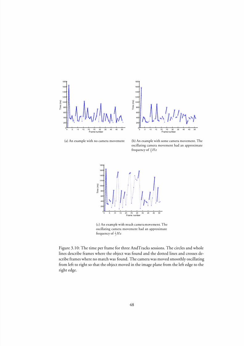
8/2/2019 Olsson Akesson Master 09
http://slidepdf.com/reader/full/olsson-akesson-master-09 52/72
8/2/2019 Olsson Akesson Master 09
http://slidepdf.com/reader/full/olsson-akesson-master-09 53/72
• Object tracking from a mounted video camera . This can be very useful to
model ows of objects or to notice when an object type is visible in the videoow. Our methods of object recognition are not optimized for this use casesince this use case is object type specic, but not object specic.
Performance increasing extensions
The implementation has promising performance increasing possibilities. Some of them are:
• Position estimation and ltering. Since the camera knows where the objecthas been previously it is possible to estimate a likely position of the object atthe current time. This can lead to the possibility to clip the input image forfaster localization, extraction and matching. A simple position estimation likeoptical ow can be used to accommodate this, or even a more advanced lteringmethod such as Kalman lters [31].
• Use of sensors to estimate position. If the device has position sensors onecan use these to increase the application performance. It can be used both toestimate the position and to cut an input image instead of or together withthe previous example or just to improve the cognitive experience of the imageoverlay on the preview area. If a rectangle is chosen to illustrate the location, onecan compensate for camera movement by moving the rectangle appropriately until a new image is available from the feature matcher. This will of course
not compensate if the object moves instead of the camera, but it could greatly improve the delay experience for small camera movements.
• Using pre dened objects to recognize. If one wants to recognize certain objectin the video stream that are perhaps not currently viewable one could teach thetracker objects that can be recognized in a manner like ArtRec and Bartendroid.The ofine nature of such techniques makes it possible to provide proven robustfeatures for better and quicker matching. Many different pictures and anglescan be used to form 3D models or just to be faster. The features can be lteredto remove unused features when compared to known video streams. This willspeed up the recognition process as well as increase the accuracy.
• Live ltering of features. The knowledge of the object is trained using a singleimage from a single angle. Just like when using pre dened objects one couldmake the features more robust even when the user selects an object if one useslive ltering. Since matches are found continuously in the video stream, it willbecome obvious which features are left unmatched. As the camera or the objectmoves the originally matching features will be less useful do to change of angles.This can be compensated by extending the known feature set with features fromdifferent angles that ought to belong to the object or by removal of features thatare no longer in the cameras point of view. This will mean that matches andspeed will increase gradually until an optimized feature set is achieved. Grading
49

8/2/2019 Olsson Akesson Master 09
http://slidepdf.com/reader/full/olsson-akesson-master-09 54/72
features and removing useless features in each step could increase performance
greatly.• Use of smaller feature descriptors. If the descriptors are of a simpler nature, one
can extract and compare features much faster. This will of course lead to morematching features, but if the inlier ltering with RANSAC is done properly, onecan probably increase the overall speed while the accuracy remains at an equallevel. It is also possible to utilize the repeating nature of a live video streamsince the same descriptors will be calculated often. Caching of descriptors forthe same feature can be done using the previously mentioned extensions.
50
8/2/2019 Olsson Akesson Master 09
http://slidepdf.com/reader/full/olsson-akesson-master-09 55/72
Chapter 4
Conclusions
4.1 Evaluation of Android as a platform for Computer Visionapplications
This thesis has proven that implementation of computer vision applications in a highlevel language such as Java on a modern mobile platform such as Android is possibleif the correct considerations are taken. Even though the Java implementations areusable for certain applications it became obvious during the process that one has toimplement some parts of the programs in native code if the applications are to work ofine with reasonable speed.
One is often constrained by the computing power of the device, but the fast net- work speed of modern mobile networks and the seamless integration of applicationsinto the Android operating system leads to the possibility to make such constraintsless visible to the end user. Handheld devices do not only put constraints compared toa desktop computer, but they also provide added functionality such as high resolutioncameras and in some cases sensors to assist calculations.
The user interface possibilities of the Android platform make it possible to keepthe user busy while calculations are processed. This lowers the perceived runtime of the calculations and gives an overall positive cognitive experience.
4.2 Future work
There are plenty of promising future possibilities for mobile computer vision withplatforms such as Android.
4.2.1 Increased computational power
The big issue is still the low computational power of mobile devices. As processorsbecome more and more power efcient, they also become useful in mobile devices. We will probably see multi core processors with equal individual core clock frequency to that we have in our single core today. One can often trace the changes in the
51

8/2/2019 Olsson Akesson Master 09
http://slidepdf.com/reader/full/olsson-akesson-master-09 56/72
desktop market a few years back to the awaiting changes in the mobile market. Many
of the computer vision algorithms can be parallelized due to the fact that the corescan operate on different parts of the processed image or matrices obtained from theimages. This opens for almost linear increase in computational power per added core.
4.2.2 Dedicated graphical processors
Certain modern mobile phones have dedicated graphical processing for 2D and 3Danimation. This can be used to speed up certain matrix calculations, as mentionedearlier in the thesis. At the time of writing there are however only mobile phones withsupport for OpenGL ES 1.0. OpenGL ES 1.0 brings very little help that is useful incomputer vision to the table. But promise lies ahead as Android will have support forOpenGL ES 2.0 [23] in the next version, named ”Donut” release of Android.
The OpenGL ES shader language (GLSL ES or ESSL) included in OpenGL ES2.0 has many built-in functions for vector and matrix operations. In many casesthese functions are SIMD (Single Instruction, Multiple Data) which can be performedelement wise operations on vectors with no extra overhead compared to a single scalaroperation.
4.2.3 Floating point processors
Since mobile devices normally lack processors with oating point operations, suchoperations have to be realized in software. This becomes a large constraint in computervision applications since many of the applications need to use millions of calculationson numbers in decimal representation. Using a VFP co-processor will make oatingpoint operations run even faster than xed point converted operations.
4.2.4 Faster mobile access with 3G LTE
With 3G Long Term Evolution (LTE) mobile access, often dubbed ”4G”, one can senddata at a much higher rate and often lower latencies. This opens up for faster seamlesstransfer to computational servers for some heavy computer vision needs. This willprobably mostly be interesting when many combined operations such as recognition of multiple bottles in a large image are needed, rather than in real time video applications.
52

8/2/2019 Olsson Akesson Master 09
http://slidepdf.com/reader/full/olsson-akesson-master-09 57/72
References
[1] Amazon Elastic Cloud Compute. Amazon elastic cloud compute.http://aws.amazon.com/documentation/ , June 2009.
[2] Android open source project. Designing for performance. http://developer.android.com/guide/practices/design/performance.html , April 2009.
[3] H. Bay, A. Ess, T. Tuytelaars, and L. Van Gool. Speeded-up robust features(surf). Computer Vision and Image Understanding , 110(3):346–359, June 2008.
[4] H. Bay, B. Fasel, and L. Van Gool. Interactive museum guide: Fast and robustrecognition of museum objects. InProceedings of the rst International Workshopon Mobile Vision, 2006.
[5] J. S. Beis and D. G. Lowe. Shape indexing using approximate nearest-neighboursearch in high-dimensional spaces. InProceedings of the IEEE Conference onComputer Vision and Pattern Recognition (CVPR), page 1000. IEEE ComputerSociety, 1997.
[6] J. L. Bentley. Multidimensional binary search trees used for associative searching.Commun. ACM , 18(9):509–517, 1975.
[7] D. Bornstein. Dalvik VM internals. InGoogle I/O Developer Conference , May 2008.
[8] P. Brady. Anatomy & physiology of an Android. InGoogle I/O Developer Con-
ference , May 2008.[9] T. H. Cormen, C. E. Leiserson, R. L. Rivest, and C. Stein.Introduction to
Algorithms, Second Edition. The MIT Press, September 2001.
[10] E. Deelman, G. Singh, M. Livny, B. Berriman, and J. Good. The cost of doingscience on the cloud: the montage example. InProceedings of the ACM/IEEE conference on Supercomputing . IEEE Press, 2008.
[11] D. A. Forsyth and J. Ponce.Computer Vision: A Modern Approach. Prentice Hall, August 2002.
53
8/2/2019 Olsson Akesson Master 09
http://slidepdf.com/reader/full/olsson-akesson-master-09 58/72
[12] J. H. Friedman, J. L. Bentley, and R. A. Finkel. An algorithm for nding best
matches in logarithmic expected time.ACM Trans. Math. Softw., 3(3):209–226,1977.
[13] G. Fritz, C. Seifert, M. Kumar, and L. Paletta. Building detection from mobileimagery using informative SIFT descriptors. InProceedings of the ScandinavianConference on Image Analysis , pages 629–638, 2005.
[14] Google App Engine project. Google app engine documentation.http://code.google.com/intl/sv-SE/appengine/docs/ , June 2009.
[15] R. Hartley and A. Zisserman.Multiple View Geometry in Computer Vision. Cam-bridge University Press, 2000.
[16] B. Kisacanin, S. S. Bhattacharyya, and S. Chai, editors.Embedded Computer Vision. Springer Publishing Company, Inc., 2008.
[17] D. G. Lowe. Object recognition from local scale-invariant features. InProceed-ings of International Conference on Computer Vision, pages 1150—1157, 1999.
[18] D. G. Lowe. Distinctive image features from scale-invariant keypoints.Interna-tional Journal of Computer Vision, 60(2):91–110, 2004.
[19] R. Meier. Professional Android application development . Wiley Publishing, inc,Indianapolis, IN, USA, 2009.
[20] A. Neubeck and L. Van Gool. Efcient non-maximum suppression. InPro-ceedings of the 18th International Conference on Pattern Recognition (ICPR), pages850–855. IEEE Computer Society, 2006.
[21] M. Ozuysal, P. Fua, and V. Lepetit. Fast keypoint recognition in ten lines of code.In Proceedings of the IEEE Conference on Computer Vision and Pattern Recognition(CVPR), 2007.
[22] T. A. O. S. Project. Dalvik bytecode verier notes. http://android.git.kernel.org/?p=platform/dalvik.git;a=blob_plain;f=docs/verifier.html;hb=HEAD , february 2009.
[23] D. Sparks. Inclusion of OpenGL ES 2.0 hardware bindings in An-droid. http://groups.google.com/group/android-developers/ msg/32de221c98196581 , February 2009.
[24] Sun Grid Engine. Sun grid engine documentation.http://www.sun.com/software/sge/techspec.xml , June 2009.
[25] D.-N. Ta, W.-C. Chen, N. Gelfand, and K. Pulli. SURFTrac: Efcient trackingand continuous object recognition using local feature descriptors. InProceed-ings of the IEEE Conference on Computer Vision and Pattern Recognition (CVPR),2009.
54

8/2/2019 Olsson Akesson Master 09
http://slidepdf.com/reader/full/olsson-akesson-master-09 59/72
[26] G. Takacs, V. Chandrasekhar, N. Gelfand, Y. Xiong, W.-C. Chen, T. Bismpi-
giannis, R. Grzeszczuk, K. Pulli, and B. Girod. Outdoors augmented reality on mobile phone using loxel-based visual feature organization. InProceedings of the 1st ACM international conference on Multimedia Information Retrieval (MIR),pages 427–434. ACM, 2008.
[27] P. van Emde Boas. Preserving order in a forest in less than logarithmic time.In Proceedings of the 16th Annual Symposium on Foundations of Computer Science (SFCS), pages 75–84. IEEE Computer Society, 1975.
[28] L. M. Vaquero, L. Rodero-Merino, J. Caceres, and M. Lindner. A break inthe clouds: towards a cloud denition.SIGCOMM Comput. Commun. Rev.,39(1):50–55, 2009.
[29] P. Viola and M. Jones. Robust real-time object detection. InInternational Journal of Computer Vision, 2001.
[30] D. Wagner, G. Reitmayr, A. Mulloni, T. Drummond, and D. Schmalstieg.Pose tracking from natural features on mobile phones. InProceedings of the 7thIEEE/ACM International Symposium on Mixed and Augmented Reality (ISMAR),pages 125–134, 2008.
[31] A. Yilmaz, O. Javed, and M. Shah. Object tracking: A survey.ACM Comput.Surv., 38(4):13, 2006.
55

8/2/2019 Olsson Akesson Master 09
http://slidepdf.com/reader/full/olsson-akesson-master-09 60/72

8/2/2019 Olsson Akesson Master 09
http://slidepdf.com/reader/full/olsson-akesson-master-09 61/72
Appendix A
Android
A.1 Introduction
Android is a complete software platform for different sorts of devices. This means thatit is an operating system and software stack to run Android specic software. It wasintroduced by Google in 2007 and is aimed at changing the way mobile applicationsare developed. The system is based on Linux and runs Java programmed applicationson top. The big difference from normal mobile Java development is that Androidsupports a large part of the Java SE1 through Apache Harmony instead of the crippled Java ME package. Android also does not use Sun’s Java Virtual Machine or even Javabyte code, but instead uses its own engine named ’Dalvik’ together with its own setof byte code. This means that Android does not run Java applications, but rather Android applications programmed in the Java language with Android extensions[19,pages 1-3].
A.2 The Linux kernel
Android is based on the Linux 2.6 kernel. Just as in any other Linux system theandroid kernel provides core system functionalities mostly linked to the hardware ab-straction [19, page 13].
Even though Android is based on a Linux kernel, it is not a GNU/Linux, which is what is normally thought of in relation to the word ’Linux’. Android does not includeall standard Linux utilities, it has no native window manager and it lacks compatibility with the standard C/C++ libraries of the GNU C library (glibc).
Android includes its own C library (libc) called Bionic. Bionic is optimized forembedded applications, with small and fast code paths and a custom implementationof POSIX threads (pthreads). Furthermore, it has built-in support for some Androidspecic features like system properties and logging. The reason that Bionic is notfully compatible with glibc that it lacks some POSIX features which are not needed in Android. These missing features are mostly concerning C++ libraries [8].
1 Java SE is the Standard Edition that is normally used on desktop platforms.
57

8/2/2019 Olsson Akesson Master 09
http://slidepdf.com/reader/full/olsson-akesson-master-09 62/72
Display driver
Keypad driver
Camera driver
WiFi driver
Flash memorydriver
Audio drivers
Binder (IPC) driver
Power management
Linux kernel
Android runtime
Core libraries
Dalvik virtualmachine
OpenGL ES
SGL
LibrariesSurface manager
FreeType
SSL
Media framework
WebKit
libc
SQLite
Location-basedservices
Telephony
Content providers
P2P/IM
Window manager
Notifications
Activity manager
Views
Application frameworkPackage manager
Resourcemanager
Developer applications
ApplicationsThird party applicationsNative applications
Figure A.1: The Android stack
58

8/2/2019 Olsson Akesson Master 09
http://slidepdf.com/reader/full/olsson-akesson-master-09 63/72
A.3 The system libraries
System libraries (written in C/C++) are exposed through the application framework and provide graphics capabilities, hardware acceleration etc. and also includes a fully functional SQL server (SQLite), SSL libraries for security, an OpenCORE based me-dia framework and WebKit for web browsing [19, page 13].
A.4 Android runtime
A.4.1 Core libraries
Android implements a core set of standard Java libraries through Apache Harmony.This means that the Android Java library set differs from Java ME in that it is notsandboxed and stripped, but is rather ’desktop Java on a small screen’. It is almost fully compatible with Java SE 1.6 except for graphical parts, but in return adds its owngraphical environment and a large collection of tting help classes and implementa-tions to speed up Android development.[19, page 13]
A.4.2 Dalvik virtual machine
Dalvik is the Virtual Machine (VM) of the Android system. It is actually technically not a Java Virtual Machine (JVM) since it comes with a whole different instructionset than a JVM would interpret. Android applications are written in Java code, butcompiled to Dalvik byte code.
Dalvik is a register based machine, as opposed to most JVMs which have a stack based structure. This structure choice will normally require larger instructions andthus often larger les, but that is not true in the case of Dalvik due to its trimmeddown VM. Dalvik will also reduce the number of CPU instructions needed per VMinstruction due to the fact that a register machine does not read from a stack and pushthe answer back but rather keeps addresses in instructions. This means that the Dalvik engine will generally be faster and load smaller les than a JVM would do. It shouldbe noted that the Dalvik engine will not do some optimizations such as loop unrollingin the manner that a normal JDK/JVM would. This means that the programmer willhave to do some extra optimizations and smart design choices [7].
A.4.3 The code verier
The local system (device) VM that loads the compiled Dalvik code (.dex) contains asystem specic verier. This verier will check that the loaded code is type safe, iscompatible with the device and also perform local and system specic optimizationsof the byte code where possible [22].
59
8/2/2019 Olsson Akesson Master 09
http://slidepdf.com/reader/full/olsson-akesson-master-09 64/72
A.5 Application framework
The application framework contains the code base for hardware interaction, the spe-cialized design patterns and other parts of the Android development methodology.The main parts are
• Activity managerhandles the activities of your application.
• Views are the building blocks of UI creation and manipulation.
• Notication manager provides different types of signaling alternatives to makethe user and device aware of changes.
• Content providers provide a simple way of sharing data between applications. A normal Android application has its own le system which cannot be ma-nipulated from other applications. Data channels are instead opened throughcontent providers.
• Resource manager handles the resources of the application. Application re-sources are entities such as UI elements, strings and other parts that can beexternalized from the code into XML les and fetched when needed [19, pages15,52-53].
A.6 The structure of an application
”All applications are created equal.”There is no difference between built-in applications and third-party applications.
It’s possible to replace core apps such as the contact list, dialer or home screen. An application can be built by one or more parts. These parts are dened in XML
and described in this section.Each application denes its permissions in the application manifest. Typical per-
missions are Internet access and camera usage. The user decides at install time if theseneeded permissions are acceptable. This means that the user will only agree to a per-mission once, but it will be granted for as long as the application is installed.
A.6.1 Activity An activity is a part of an application which displays a graphical interface of some sortand can retrieve input from the user. Most applications will be made of a collectionof activities. These activities contain views to display information. A very simpleexample of an activity can be seen in ListingA.1.
A.6.2 Service
Activities can contain services. Services are background processes which can run dur-ing a long period of time. These will most often sleep when there is nothing to be
60

8/2/2019 Olsson Akesson Master 09
http://slidepdf.com/reader/full/olsson-akesson-master-09 65/72
done and process information when wanted. This is somewhat like the concept of
”server daemons” in Unix. An example of a service use case would be donwloading weather information for display in a widget.
Listing A.1: Basic activity stubpublic classMyActivity extends Activity {
/∗∗Called when the activity is rst created.∗/@Overridepublic void onCreate(Bundle savedInstanceState){
super.onCreate(savedInstanceState);setContentView(R.layout.main);
}}
A.6.3 Broadcast receiver
A broadcast receiver receives and may answer specic events. Broadcast receivers mustprocess very quickly and are used as small background services which can run whencalled. An example would be a broadcast receiver which receives an event which saysthat a photo has been taken and logs this to a specic le.
A.6.4 Content providers
Android applications do not share a le system beyond data saving on an SD card.
Content providers are meant to serve applications with useful data of specic sorts.This data can for example be contacts in a phone book, bookmarks from a web browseretc.
A.7 The life cycle of an application
A.7.1 Intents
Applications are started from a system called ”Intents”. Intents dene that an applica-tion is capable of handling a job. That job can be for example ”viewing a web page”,”calling a phone number” or ”sending a text message”. When one application wantsto perform a task that another application should implement it sends out an intent. If there is an application that can handle the intent it will be started. If there are morethan one application that can handle an intent, one will get a menu to choose from orthe preferred one will be selected automatically depending on the situation. Explicitstaring of an application from for example an application menu is done by sending aspecic intent to start said application.
A.7.2 Knowing the state of an application
Android applications need to keep track of their state at all times. Instead of explicitly starting and stopping applications, the system is designed to be able to pause appli-
61

8/2/2019 Olsson Akesson Master 09
http://slidepdf.com/reader/full/olsson-akesson-master-09 66/72
cations when they are not displayed and later possibly bring them back. This means
that an application has to save its state when it gets a pause command or data mightbe lost if Android decides to shut down the application in order to save memory orbattery power.
If an application does not correctly pause its execution when told to it will con-tinue to run in background until it might be killed at any time without any further warning. This behavior makes it very simple to resume a session from the previously run since paused applications will keep their memory space until some other applica-tion claims it. It can also have the effect that applications will become useless whenresumed unless rst explicitly killed and later started again since clicking a ”back” but-ton or similar and starting the application again will not have the expected effect of anapplication restart unless the applications is designed for this behavior.
62

8/2/2019 Olsson Akesson Master 09
http://slidepdf.com/reader/full/olsson-akesson-master-09 67/72
Appendix B
Distributed computing in The
Cloud”The Cloud” is a metaphor for the Internet. The metaphor has become popular asof late to describe the fact that the user does not know where in the world his data issent or received, nor should he or she need to know that [28]. Cloud computing hasemerged as an alternative to the traditional setup of servers at local companies, schoolsetc. Instead of having the need to have a powerful server which is unused duringlong times one can rent computing power and bandwidth from a cloud computingservice. This can be compared to super computers, but with the added possibility of fast internet access to users from around the world and the possibility to seamlessly scale the application as the user base or application evolves.
This type of setup leads to more efcient power usage, less server technicians anda system which can evolve and expand organically at a predictable cost.
Many different companies offer cloud computing services with some difference intarget groups.
B.1 Cloud computing services
B.1.1 Amazon Elastic Compute Cloud (EC2)
The Amazon Elastic Computer cloud is a system where the user is granted one or morevirtual servers to congure and run as one pleases[1]. To start a server one can chooseamong a list of common systems such as different Linux distributions and Microsoft Windows setups. A suitable hardware setup is chosen to accompany this softwaresetup. The server can thereafter be started and congured as suitable. The system canbe started in a data center in the USA or Europe depending on the administrator’schoice.
A large difference from a normal server setup is that the virtual server has its datasaved only when it is running. As the server is terminated it will no longer exist,and also not cost anything. This adds the possibility to start up a large number of new servers for whatever need the administrator might have. One must however remember
63
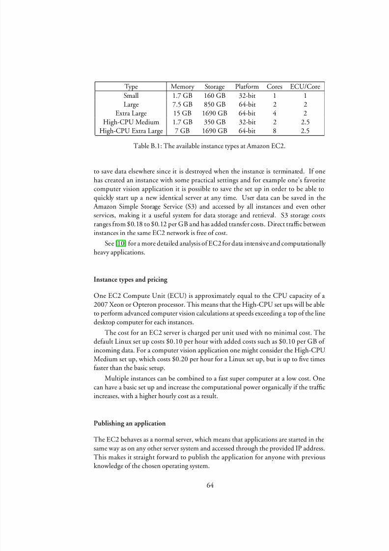
8/2/2019 Olsson Akesson Master 09
http://slidepdf.com/reader/full/olsson-akesson-master-09 68/72
Type Memory Storage Platform Cores ECU/Core
Small 1.7 GB 160 GB 32-bit 1 1Large 7.5 GB 850 GB 64-bit 2 2
Extra Large 15 GB 1690 GB 64-bit 4 2High-CPU Medium 1.7 GB 350 GB 32-bit 2 2.5
High-CPU Extra Large 7 GB 1690 GB 64-bit 8 2.5
Table B.1: The available instance types at Amazon EC2.
to save data elsewhere since it is destroyed when the instance is terminated. If onehas created an instance with some practical settings and for example one’s favoritecomputer vision application it is possible to save the set up in order to be able toquickly start up a new identical server at any time. User data can be saved in the Amazon Simple Storage Service (S3) and accessed by all instances and even otherservices, making it a useful system for data storage and retrieval. S3 storage costsranges from $0.18 to $0.12 per GB and has added transfer costs. Direct trafc betweeninstances in the same EC2 network is free of cost.
See [10] for a more detailed analysis of EC2for data intensive and computationally heavy applications.
Instance types and pricing
One EC2 Compute Unit (ECU) is approximately equal to the CPU capacity of a2007 Xeon or Opteron processor. This means that the High-CPU set ups will be ableto perform advanced computer vision calculations at speeds exceeding a top of the linedesktop computer for each instances.
The cost for an EC2 server is charged per unit used with no minimal cost. Thedefault Linux set up costs $0.10 per hour with added costs such as $0.10 per GB of incoming data. For a computer vision application one might consider the High-CPUMedium set up, which costs $0.20 per hour for a Linux set up, but is up to ve timesfaster than the basic setup.
Multiple instances can be combined to a fast super computer at a low cost. Onecan have a basic set up and increase the computational power organically if the trafcincreases, with a higher hourly cost as a result.
Publishing an application
The EC2 behaves as a normal server, which means that applications are started in thesame way as on any other server system and accessed through the provided IP address.This makes it straight forward to publish the application for anyone with previousknowledge of the chosen operating system.
64

8/2/2019 Olsson Akesson Master 09
http://slidepdf.com/reader/full/olsson-akesson-master-09 69/72
B.1.2 Sun Grid Engine
Sun Grid Engine is a cloud computing system operated by Sun, which mainly focuseson batch jobs and other computationally intensive applications[24]. Grid is useful forscientic calculations and for example video rendering, but not for end user distribu-tion. Large computations that will take hours or days to run on a desktop computercan be sent to the Grid for faster calculation as long as the application follows certainrules, such as the ability to run on the Solaris 10 operating system and an applicationsize below 10 GB.
Pricing
Sun Grid computing is charged per CPU hour. Each hour costs $1. The calculationsare not limited to a single CPU, but can be run as fast as needed with the cost basedon the number of CPUs used. This means that if the application uses 60 CPUs forone minute it is charged as one hour.
Publishing an application
Sun Grid calculations are published to the Grid as batch jobs. A shell script thatcontrols the data ows is specied together with the needed arguments for said script.The applications themselves need sometimes not implement much computation, butrather reference one of the many available libraries for computation and rendering,
such as Calculix, Fractal and Blender.
B.1.3 Google App Engine
Google App Engine is a cloud computing system operated by Google, which focuseson web applications that run in a limited time span[14]. Web applications on AppEngine can be programmed in the Java or Python languages with simple support formodern Web 2.0 interfaces through Google Web Toolkit (GWT). This makes it suit-able for scalable web applications, but less attractive for computer vision applications. Applications on the App Engine need to be accessed through the World Wide Weband are strictly limited in the choices of programming languages and other libraries.
There are hard limits on request times and transfer sizes, making App Engine unsuit-able for intense calculations.
Pricing
App Engine differs from Amazon EC2 and Sun Grid in that the basic system is freeof charge, with the added possibility of higher limits at a price. The free setup willstop working when certain limits are met. The price of added computational poweris $.10-$.12 per CPU hour and $0.10 per incoming GB of data. Some limits are notpossible to overcome even with a non-free plan.
65

8/2/2019 Olsson Akesson Master 09
http://slidepdf.com/reader/full/olsson-akesson-master-09 70/72
Publishing an application
A web application for App engine is pushed to the service using Google’s providedsoftware. No explicit server conguration is needed, or possible. The user is given a web address where the application can be accessed as web page.
B.1.4 Discussion
This section has discussed various systems for cloud computing. The three providedexamples will often differ greatly in application development and execution, whichmeans that one ought to take note of where the application is to be run prior todevelopment start.
In this thesis we have used the Amazon Elastic Compute Cloud (EC2) for the
Bartendroid server in Section3.3.2. This was a choice that grew out of the interestto investigate an industry size system and the possibilities of distribution. Using EC2is excellent for a service, since one can congure the host system as needed and thusrun most applications that are wanted. This means that the EC2 can have support forlegacy code if it is congured to have that.
Our position is that the EC2 is the best solution for services that rely on heavy computing, while Sun Grid is the best solution for very heavy batch jobs such asrendering and Google App Engine is most suitable for web based applications that will nish within a limited time. Due to the advanced possibilities and APIs of AppEngine, one can for example build a web application that calls EC2 for some heavy cal-culations and otherwise makes due with the available power of the App Engine. Our
systems have not used web based access for the computer vision part, but it is prob-able that many applications will do that in order to get easy access to the applicationregardless of calling device type and operating system.
66

8/2/2019 Olsson Akesson Master 09
http://slidepdf.com/reader/full/olsson-akesson-master-09 71/72

8/2/2019 Olsson Akesson Master 09
http://slidepdf.com/reader/full/olsson-akesson-master-09 72/72
M t ’ Th i M th ti l S i 2009 E22