NUMERICAL SOLUTION OF THREE DIMENSIONAL CONJUGATE HEAT...

NUMERICAL SOLUTION OF THREE

DIMENSIONAL CONJUGATE HEAT TRANSFER IN

A MICROCHANNEL HEAT SINK AND CFD

ANALYSIS

A THESIS SUBMITTED IN PARTIAL FULFILLMENT OF THE

REQUIREMENTS FOR THE DEGREE OF

Bachelor of Technology

in

Mechanical Engineering

BY

AMRITRAJ BHANJA

DEPARTMENT OF MECHANICAL ENGINEERING

NATIONAL INSTITUTE OF TECHNOLOGY

ROURKELA-769008

2009

NUMERICAL SOLUTION OF THREE

DIMENSIONAL CONJUGATE HEAT TRANSFER IN

A MICROCHANNEL HEAT SINK AND CFD

ANALYSIS

A THESIS SUBMITTED IN PARTIAL FULFILLMENT OF THE

REQUIREMENTS FOR THE DEGREE OF

Bachelor of Technology

in

Mechanical Engineering

BY

AMRITRAJ BHANJA

Under the guidance of

Dr. ASHOK KUMAR SATAPATHY



ROURKELA-769008

2009


ROURKELA

CERTIFICATE

This is to certify that the thesis entitled “NUMERICAL SOLUTION OF THREE

DIMENSIONAL CONJUGATE HEAT TRANSFER IN A MICROCHANNEL HEAT SINK

AND CFD ANALYSIS” submitted by Sri Amritraj Bhanja in partial fulfillment of the

requirements for the award of Bachelor of technology Degree in Mechanical

Engineering at the National Institute of Technology, Rourkela (Deemed University) is an

authentic work carried out by him under my supervision and guidance.

To the best of my knowledge, the matter embodied in the thesis has not been

submitted to any other University / Institute for the award of any Degree or Diploma.

DATE: DR. ASHOK KUMAR SATAPATHY



ROURKELA-769008

National Institute of Technology

Rourkela

ACKNOWLEDGEMENT

I would like to express my deep sense of gratitude and respect to my supervisor

Prof. Ashok Kumar Satapathy, for his excellent guidance, suggestions and constructive

criticism. I consider myself extremely lucky to be able to work under the guidance of

such a dynamic personality.

I would like to render heartiest thanks to our M.Tech students(ME) whose ever

helping nature and suggestion has helped us to complete this present work

DATE: AMRITRAJ BHANJA

ROLL NO 10503071, B.TECH



ROURKELA-769008

DEPARTMENT OF MECHANICAL ENGINEERING,

NIT ROURKELA Page i

CONTENTS

Contents…………………………………………………………………………………………….. i

Abstract……………………………………………………………………………………………. ii

List of Figures………………………………………………………………………………….. iii

1. Introduction

1.1 Micro-channel Heat Sink…………………………………………………...2

1.2 About the Project…………………………………………………………….. ..4

1.3 GAMBIT-FLUENT………………………………………………………………..5

2. Theory

2.1 Heat Transfer by Conduction ………………........................................8

2.2 Heat Transfer by Radiation………………………………………………...8

2.3 Heat Transfer by Convection………………………………………………8

2.3.1Reynolds Number.................................................................... 9

2.3.2 Nusselt Number.......................................................................9

2.3.3 Prandtl Number.......................................................................9

2.3.4 Grashof Number.................................................................. 10

2.3.5 Rayleigh Number………………………………………………….10

2.4 Computational Fluid Dynamics & FLUENT………………………..10

3. Design of SINGLE Micro-channel in GAMBIT............................................14

4. Fluent analysis of Micro-channel.................................................................18

5. Results and Discussions..................................................................................24

6. Conclusion...........................................................................................................36

7. Application of CFD............................................................................................37

Bibliography............................................................................................................38


NIT ROURKELA Page ii

ABSTRACT

In electronic equipments, thermal management is indispensable for its longevity and

hence, it is one of the important topics of current research. The dissipation of heat is

necessary for the proper functioning of these instruments. The heat is generated by the

resistance encountered by electric current. This has been further hastened by the

continued miniaturization of electronic systems which causes increase in the amount of

heat generation per unit volume by many folds. Unless proper cooling arrangement is

designed, the operating temperature exceeds permissible limit. As a consequence,

chances of failure get increased.

Increasing circuit density is driving advanced cooling systems for the next generation

microprocessors. Micro-Channel heat exchangers (MHE) in silicon substrates are one

method that is receiving considerable attention. These very fine channels in the heat

exchanger provide greatly enhanced convective heat transfer rate and have been shown

to be able to meet the demands of the cooling challenge for the microprocessors for

many generations to come.

This work focused on laminar flow (Re < 200) within rectangular micro-channel with

hydraulic diameter 86µm for single-phase liquid flow. The influence of the thermo-

physical properties of the fluid on the flow and heat transfer, are investigated by

evaluating thermo-physical properties at a reference bulk temperature. The micro-heat

sink model consists of a 10 mm long silicon substrate, with rectangular micro-channels,

57µm wide and 180µm deep, fabricated along the entire length. Water at 293k is taken

as working fluid. The results indicate that thermo-physical properties of the liquid can

significantly influence both the flow and heat transfer in the micro-channel. Assumption

of hydrodynamic, fully developed laminar flow is valid here on basis of Langhaar’s

equation. The local heat transfer coefficient and averaged Nusselt number is calculated

and plotted for pressure drop of 50kpa, 30kpa and 10kpa. The result is verified for heat

flux 50w/cm2, 90w/cm2 and 150w/cm2. A three-dimensional Computational Fluid

Dynamics (CFD) model was built using the commercial package, GAMBIT-FLUENT, to

investigate the conjugate fluid flow and heat transfer phenomena.


NIT ROURKELA Page iii

LIST OF FIGURES

Fig 1 Structure of Micro-channel Heat Sink Page 5

Fig 2 Schematic diagram of single Micro-channel Page 25

Fig 3 Temperature contour of Outlet at 50 w/cm2, 50 KPA Page 25

Fig 4 Temperature contour of Outlet at 90 w/cm2, 50 KPA Page26


Fig 6 Velocity Contour at 50 KPa Page 27

Fig 7 Graph of Nu vs Z at 50 Kpa Page 27

Fig 8 Graph of Nu vs Re at 50 Kpa Page 28




Fig 12 Velocity Contour at 30 KPa Page 30

Fig13 Graph of Nu vs Re at 30 Kpa Page 30

Fig 14 Graph of Re vs Z Page 31

Fig 15 Schematic diagram of double Micro-channel Page 31

Fig 16 Temperature contour of Outlet at 50 w/cm2, 50 KPA,

adiabatic wall conditions Page 32

Fig 17 Temperature contour of Outlet at 50 w/cm2, 50 KPA,

Isothermal wall conditions Page 32

Fig 18 Velocity Contour of Outlet Page 33


NIT ROURKELA Page 1

CHAPTER 1

INTRODUCTION

� MICROCHANNEL HEAT SINK

� ABOUT THE PROJECT

� GAMBIT-FLUENT


NIT ROURKELA Page 2

1. INTRODUCTION

1.1. MICROCHANNEL HEAT SINKS:

Advance in micromachining technology in recent years has enabled the design

and development of miniaturized systems, which opens a promising field of

applications, particularly in the medical science and electronic-/bioengineering.

Such systems often contain small scale fluid channels embedded in the

surrounding solids with heating sources. Depending on the channel height, it can

be described as a Mini-channel (at a characteristic dimension of about 1 mm) or

a Micro-channel (at a characteristic dimension of several microns to several

hundred microns). Because of its undeniable advantages of smaller physical

dimensions and higher heat transfer efficiency, the study of micro-channel flows

has become an attractive research topic with a fast-growing number of

publications. Micro-scale heat transfer has received much interest as the size of

the devices decreases, such as in electronic equipments, since the amount of heat

that needs to be dissipated per unit area increases. The performance of these

devices is directly related to the temperature; therefore it is a crucial issue to

maintain the electronics at acceptable temperature levels. Micro-channel heat

sinks have become known as one of the effective cooling techniques. The design

of next generation, giga-scale integrated circuits, requires effective cooling for

reliable, long term operations. These devices may even experience catastrophic

failure due to generation of very high heat flux (VHHF) transients. The VHHF

transients originate from hot spots which may be difficult to localize at all times

and will be difficult to handle using conventional cooling techniques. Micro-

channel heat-sinks have thus emerged as a promising cooling solution due to

high heat transfer coefficient derived from a large surface area to volume ratio.

Micro-channel cooling technology was first put forward by Tuckerman and

Pease[1]. They circulated water in micro-channel fabricated in silicon chips and

were able to reach a heat flux of 790w/cm2 without a phase change in a pressure

drop of 1.94 bar. Shortly after, Wu and Little [2] obtained experimental results


NIT ROURKELA Page 3

for fluid flow in micro-channels for gas flow. Their measured friction factors in

the laminar regime were higher than expected and they found that the transition

Reynolds number ranged from 350 to 900. Peng [3] conducted experiments on

micro-channels and they found that the laminar-to-turbulent transition period

occurred at Reynolds numbers which were lower than expected from

conventional theory. Peng and Peterson found disparities between conventional

flow theory and experimental results for micro-channels. They tested micro-

channels with hydraulic diameters ranging from 133 μm to 367 μm, and they

showed a friction factor dependence on hydraulic diameter and channel aspect

ratio [4]

Judy et al. [5] did pressure drop experiments on both round and square micro-

channels with hydraulic diameters ranging from 15 to 150 μm. They tested

distilled water, methanol and iso-propanol over a Reynolds number range of 8 to

2300. Their results showed no distinguishable deviation from laminar flow

theory for each case. Liu and Garimella [6] conducted flow visualization and

pressure drop studies on micro-channels with hydraulic diameters ranging from

244 to 974 μm over a Reynolds number range of 230 to 6500. They compared

their pressure drop measurements with numerical calculations. Computations

were performed for different total pressure drops in the channel to obtain the

relation between the overall averaged Nu number and the Re number for this

specific geometry of heat sinks. Choi et al. [7] also suggested by their

experiments with micro-channels inside diameters ranging from 3 to 81µm that

the Nusselt number did in fact depend on the Reynolds number in laminar

micro-channel flow. Experimental measurements for pressure drop and heat

transfer coefficient were done by rahman[8]. He used water as a working fluid

and tests were conducted on channels of different depths.

Fedorov and Viskanta [9] investigate the conjugate heat transfer in a

microchannel heat sink .they found that the average channel wall temperature

along the flow direction was nearly uniform except in the region close to the

channel inlet, where very large temperature gradients were observed.


NIT ROURKELA Page 4

1.2. ABOUT THE PROJECT:

In the present study a numerical model with fully developed flow is presented

and used to analyze a three dimensional micro-channel heat sink for Re numbers

(< 160) and with hydraulic diameter 86 µm. In the current investigation, three

different cases (Qw = 90, W/cm2, ∆P = 50, 15, and 10kPa) were considered. Also,

it was analyzed for a heat flux of 50, 90 and 150W/cm2 .The numerical model is

based on three dimensional conjugate heat transfer FLUENT, a commercial

package employing continuum model of Navier Stokes equation with SIMPLE

algorithm. The numerical solver codes are well-established and thus provide a

good start to more complex heat transfer and fluid flow problems. FLUENT

provides adaptability to variation of thermo physical properties with respect to

temperature effect. The thermo physical properties are chosen at a reference

temperature A series of calculations were carried out to analyze rectangular

silicon-based micro-channel heat sink. Computations were performed for

different total pressure drops in the channel to obtain the relation between the

overall averaged Nu number and the Re number for this specific geometry of

heat sinks.

Here the micro-heat sink model consists of a 10 mm long substrate and

dimension of rectangular micro-channels have a width of 57 µm and a depth of

180 µm as shown in fig [1]. The heat sink is made from silicon and water is used

as the cooling fluid. The electronic component is idealized as a constant heat flux

boundary condition at the heat sink bottom wall. Heat transport in the unit cell is

a conjugate problem which combines heat conduction in the solid and convective

heat transfer to the coolant (water). Here we consider a rectangular channel of

dimension (900µx100µmx10mm) applied constant heat flux of 90w/cm2 from

bottom. Water flows through channel at temperature 293k on account of

pressure loss of 50kpa.

Here we assumed to have a constant heat flux, q”(90W/cm2 ) at the bottom wall

The other wall boundaries of the solid region are assumed to be either perfectly

Insulated with zero heat flux or at isothermal conditions. The water flow


NIT ROURKELA Page 5

velocities are taken from different Reynolds numbers, from 96 to 164, with

reference to the hydraulic diameter of 86 µm.

FIG. 1 Structure of Micro-channel Heat Sink

1.3. GAMBIT-FLUENT:

Preprocessing is the first step in building and analyzing a flow model. It includes

building the model (or importing from a CAD package), applying the mesh, and

entering the data. We used Gambit as the preprocessing tool in our project.

GAMBIT is a software package designed to help analysts and designers build and

mesh models for computational fluid dynamics (CFD) and other scientific

applications. GAMBIT receives user input by means of its graphical user interface

(GUI).

The GAMBIT GUI makes the basic steps of building, meshing, and assigning zone

types to a model simple and intuitive, yet it is versatile enough to accommodate a

wide range of modeling applications. The advantages of using gambit for the

geometry design are:


NIT ROURKELA Page 6

� Ease of use

� CAD/CAE Integration

� Fast Modeling

� CAD Cleanup

� Intelligent Meshing.

FLUENT is a computer program for modeling fluid flow and heat transfer in

complex geometries. FLUENT provides complete mesh flexibility, including the

ability to solve flow problems using unstructured meshes that can be generated

about complex geometries with relative ease. Supported mesh types include 2D

triangular/quadrilateral, 3D tetrahedral/hexahedral/pyramid/wedge, and

mixed (hybrid) meshes. FLUENT also allows you to refine or coarsen your grid

based on the flow solution.

FLUENT is written in the C computer language and makes full use of the

flexibility and power offered by the language. Consequently, true dynamic

memory allocation, efficient data structures, and flexible solver control are all

possible. In addition, FLUENT uses a client/server architecture, which allows it

to run as separate simultaneous processes on client desktop workstations and

powerful computer servers. All functions required to compute a solution and

display the results are accessible in FLUENT through an interactive, menu-driven

interface.


NIT ROURKELA Page 7

CHAPTER 2

THEORY

� HEAT TRANSFER

� CFD & FLUENT


NIT ROURKELA Page 8

2. THEORY

2.1. HEAT TRANSFER:

Heat is defined as energy transferred by virtue of temperature difference or

gradient. Being a vector quantity, it flows with a negative temperature gradient.

In the subject of heat transfer, it is the rate of heat transfer that becomes the

prime focus. The transfer process indicates the tendency of a system to proceed

towards equilibrium. There are 3 distinct modes in which heat transfer takes

place:

2.1.1. Heat transfer by Conduction:

Conduction is the transfer of heat between 2 bodies or 2 parts of the same body

through molecules. This type of heat transfer is governed by Fourier`s Law which

states that – “Rate of heat transfer is linearly proportional to the temperature

gradient”. For 1-D heat conduction-

dx

dTkqk −=

2.1.2. Heat transfer by Radiation:

Thermal radiation refers to the radiant energy emitted by the bodies by virtue of

their own temperature resulting from the thermal excitation of the molecules. It

is assumed to propagate in the form of electromagnetic waves and doesn’t

require any medium to travel. The radiant heat exchange between 2 gray bodies

at temperature T1 and T2 is given by:

)( 42

4121121 TTFAQ −= −− σ

2.1.3. Heat transfer by Convection:

When heat transfer takes place between a solid surface and a fluid system in

motion, the process is known as Convection. When a temperature difference


NIT ROURKELA Page 9

produces a density difference that results in mass movement, the process is

called Free or Natural Convection.

When the mass motion of the fluid is carried by an external device like

pump, blower or fan, the process is called Forced Convection. In convective heat

transfer, Heat flux is given by:

)()( ∞−= TThxq wx

2.1.3.1. Reynold`s Number:

It is the ratio of inertial forces to the viscous forces. It is used to

identify different flow regimes such as Laminar or Turbulent.

ForcesViscous

ForcesInertialVDVDRe ===

νµρ

2.1.3.2. Nusselt Number:

The nusselt number is a dimensionless number that measures the

enhancement of heat transfer from a surface that occurs in a real

situation compared to the heat transferred if just conduction

occurred.

fL k

hLNu =

2.1.3.3. Prandtl Number:

It is the ratio of momentum diffusivity (viscosity) and thermal

diffusivity.

αν=Pr


NIT ROURKELA Page 10

2.1.3.4. Grashof Number:

It is the ratio of Buoyancy force to the viscous force acting on a

fluid.

2.1.3.5. Rayleigh Number:

It is the product of Grashof number and Prandtl number. It is a

dimensionless number that is associated with buoyancy driven

flow i.e. Free or Natural Convection. When the Rayleigh number is

below the critical value for that fluid, heat transfer is primarily in

the form of conduction; when it exceeds the critical value, heat

transfer is primarily in the form of convection.

2.2. COMPUTATIONAL FLUID DYNAMICS (CFD) & FLUENT:

Computational fluid dynamics (CFD) is one of the branches of fluid mechanics

that uses numerical methods and algorithms to solve and analyze problems that

involve fluid flows. The fundamental basis of any CFD problem is the Navier-Stokes

equations, which define any single-phase fluid flow. These equations can be simplified

by removing terms describing viscosity to yield the Euler equations. Further

simplification, by removing terms describing vorticity yields the full potential equations.

Finally, these equations can be linearized to yield the linearized potential equations.

2

3)(

νβ LTTg

Gr s ∞−=



2.2.1. Governing equations:

Continuity Equation:

0.).( =∇+=∇+∂∂

VDt

DV

t

p ρρρ

Conservation of Momentum equation for an incompressible fluid is:

( )ux

Pg

Dt

Dux .2∆+

∂∂−= µρρ

Energy Equation:

2.2.2. Discretization Methods:

The stability of the chosen discretization is generally established numerically

rather than analytically as with simple linear problems. Special care must also be

taken to ensure that the discretization handles discontinuous solutions

gracefully. The Euler equations and Navier-Stokes equations both admit shocks,

and contact surfaces. Some of the discretization methods being used are:

2.2.2.1. FINITE VOLUME METHOD:

This is the "classical" or standard approach used most often in

commercial software and research codes. The governing equations

are solved on discrete control volumes. This integral approach

yields a method that is inherently conservative (i.e., quantities

such as density remain physically meaningful)



Where Q is the vector of conserved variables, F is the vector of

fluxes (see Euler equations or Navier-Stokes equations), V is the

cell volume, and is the cell surface area.

2.2.2.2. FINITE ELEMENT METHOD:

This method is popular for structural analysis of solids, but is also

applicable to fluids. The FEM formulation requires, however,

special care to ensure a conservative solution. The FEM

formulation has been adapted for use with the Navier-Stokes

equations. In this method, a weighted residual equation is formed:

Where Ri is the equation residual at an element vertex i , Q is the

conservation equation expressed on an element basis, Wi is the

weight factor and Ve- is the volume of the element.

2.2.2.3. FINITE DIFFERENCE METHOD:

This method has historical importance and is simple to program. It

is currently only used in few specialized codes. Modern finite

difference codes make use of an embedded boundary for handling

complex geometries making these codes highly efficient and

accurate. Other ways to handle geometries are using overlapping-

grids, where the solution is interpolated across each grid.

Where Q is the vector of conserved variables, and F, G, and H are

the fluxes in the x, y, and z directions respectively.

2.2.3. Schemes to Calculate Face Value for variables:

2.2.3.1. Central Difference scheme:

This scheme assumes that the convective property at the interface

is the average of the values of its adjacent interfaces.



2.2.3.2. The UPWIND scheme:

According to the upwind scheme, the value of the convective

property at the interface is equal to the value at the grid point on

the upwind side of the face. It has got 3 sub-schemes i.e. 1st order

upwind which is a 1st order accurate, 2nd order upwind which is 2nd

order accurate scheme and QUICK (Quadratic Upwind

Interpolation for convective kinematics) which is a 3rd order

accurate scheme.

2.2.3.3. The EXACT solution;

According to this scheme, in the limit of zero Peclet number, pure

diffusion or conduction problem is achieved and φ vs x variation is

linear. For positive values of P, the value of φ is influenced by the

upstream value. For large positive values, the value of φ seems to

be very close to the upstream value.

2.2.3.4. The EXPONENTIAL scheme:

When this scheme is used, it produces exact solution for any value

of Peclet number and for any value of grid points. It is not widely

used because exponentials are expensive to compute.

2.2.3.5. The HYBRID scheme:

The significance of hybrid scheme can be understood from the fact

that (i) it is identical with the Central Difference scheme for the

range -2<=Pe<=2 (ii) outside, it reduces to the upwind scheme.



CHAPTER 3

MICROCHANNEL MODELING USING

GAMBIT



DESIGN OF SINGLE MICROCHANNEL

USING GAMBIT STEP 1 Select a solver:

Main Menu>Solver>Fluent 5/6.

STEP 2 Creation of Vertices:

Operation>Geometry>Vertex Command Button>Create Vertex from

Co-ordinates.

The following vertices with the required Cartesian co-ordinates were

created. All dimensions are in ‘um’

Vertices Cartesian Co-ordinates

A -50,-450,0

B 50,-450,0

C 50,450,0

D -50,450,0

P -28.5,0,0

Q -28.5,-180,0

R 28.5,-180,0

S 28.5,0,0

0 50,-450,10000

STEP 3 Creation of Line:

Operation>Geometry>Creating Edge>Straight.

Create straight lines by joining the following vertices

AB,BC,CD,DA,PQ,QR,RS,SP,DO.

STEP 4 Creation of Faces:

Operation>Geometry>Face Command Button>Form Face>Create

Face from Wireframe.

To create face ‘ABCD’, select edges in a sequence order (AB>BC>CD>DA)

and click apply. Similarly, create PQRS using the same above commands.

STEP 5 Meshing Edges (PQ, QR, RS, SP):

(a) Operation>Mesh>Mesh edges.

Select Edge-PQ,RS



Grading-Apply

Type-Successive ratio.

Ratio-1.05 (Double sided)

Spacing-Apply

Interval Count- 90

Mesh-Apply

Click Apply.

(b) Select edge- QR, SP

Grading-Apply.

Type-Successive Ratio.

Ratio-1.05 (Double sided)

Spacing-Apply

Interval Count-28

Mesh-Apply

Click Apply.

STEP 6 Subtract faces.

Operation>Geometry>Face Command Button>Boolean

operations>Subtract.

Subtract face PQRS from ABCD.

STEP 7 Mesh face.

Operation>Mesh Command Button>Face mesh>Mesh faces.

Faces- Select face 1

Elements- Quad.

Type- Pave

Interval Size- 2

STEP 8 Face Creation and meshing.

Again, create a face PQRS by joining the sides PQ, QR, RS, SR.

Mesh PQRS by following the above meshing method with an interval size

of 2. The scheme should be Pave mesh.

STEP 9 Meshing Edge DO:

Operation>Mesh>Mesh Edges.

Select Edge-BH

Grading-Apply



Type-Successive ratio.

Ratio-1

Spacing-Apply

Interval Count-20

Mesh-Apply

Click Apply

STEP 10 Creation of Volume:

Operation>Geometry>Volume>Form Volume>Sweep Real Faces.

Select all the faces.

Path-Edge.

Edge-Select Line DO with mesh.

Click Apply.

STEP 11 Creating Zones.

Operation>Zones Command Button>Specify Boundary Types.

Name Type

Inlet sink Wall

Channel inlet Mass flow inlet

Heat flux Wall

Base channel Wall

Channel right Wall

Channel left Wall

Sink right Wall

Channel top Wall

Sink left Wall

Sink top Wall

Sink outlet Wall

Channel outlet Outflow

STEP 12 Creation of Continuum.

Operation>Zones Command Button>Specify Continuum Types.

Name Type

Heat sink Solid

Channel Liquid

STEP 13 File>Save as [name]

STEP 14 File>export>Mesh[File name]



CHAPTER 4

FLUENT ANALYSIS

OF

MICROCHANNEL



ANALYSIS OF MICROCHANNEL IN FLUENT:

STEP 1 Select FLUENT 3ddp.

STEP 2 Reading of the mesh file.

File>Read>Case.

STEP 3 ANALYSIS OF GRID.

a) Checking of grid

Grid>Check.

It was checked that the total volume doesn’t come as negative.

b) Scaling of Grid.

Grid>Scale.

Scale was set to 1e-6 in X, Y, Z directions.

c) Smoothing and Swapping.

Grid>Smooth/swap.

The grid was swapped until Zero faces were moved.

STEP 4 SELECTION OF MODELS.

(a) Defining solver.

DEFINE>MODELS>SOLVER.

Solver is segregated

Implicit formulation

Space steady

Time steady

(b) Define Energy Equation.

DEFINE > MODEL >ENERGY.

(c) Selection of Materials.

DEFINE > MATERIALS.



Fluid was taken to be liquid water which was selected from the fluent

database.

Solid was changed to SILICON whose properties were:

Density, = 2330 Kg/m3.

Specific Heat Capacity, k= 714 J/Kg/˚C.

Thermal Conductivity, Cp= 140

(d) Defining Operating Conditions.

DEFINE > OPERATING CONDITIONS. Operating pressure= 101.325 KPa

Gravity = -9.81 m/s2 in Y-direction

(e) Defining Boundary Conditions.

1. Channel Inlet.

Input the following values at Mass Flow Inlet.

Mass Flow Rate- 1e-5/ 6e-6 Kg/s

Temperature- 293 K

Component of X and Y velocity Direction- 0

Component of Z velocity Direction- 1

2. Heat Flux.

Input the following values at Wall.

Select Heat Flux from the list.

Heat Flux = 50/90/150 e4 W/m2.

Thickness = 450e-6 m

Click on shell conduction.

3. Channel left.



Heat Flux = 0 W/m2.

Thickness = 21.5e-6 m

Click on shell conduction



4. Channel right.



Heat Flux = 0 W/m2.

Thickness = 21.5e-6 m


5. Channel top.



Heat Flux = 0 W/m2.

Thickness = 450e-6 m


STEP 5 SELECTION OF SOLUTION.

(a) Defining Solutions. SOLVE > CONTROLS>SOLUTIONS Flow and energy equations used.

Pressure-Velocity Coupling- SIMPLE.

Under relaxation factors:

Pressure= 0.3

Density= 1

Body Force= 1

Momentum= 0.08

Energy= 1

Discretization:

Pressure= Standard.

Momentum= 2nd order upwind.

Energy= 2nd order upwind.

(b) Initializing the Solution.

The Problem was computed taking the values from all zones.



(c) Defining Monitors.

SOLVE > MONITORS>RESIDUALS.

Plot option was clicked.

Plotting was done in window 1 with 1000 iterations.

Convergence criterion:

Continuity= 0.0001

X-velocity= 0.0001

Y-velocity= 0.0001

Z- Velocity= 0.0001

Energy= 1e-8.

(d) Iterating the solution.

SOLVE >ITERATE.

No. of iterations=500.

Iterate till the solution is converged.

STEP 6 Plotting of Contours and Graphs.

(a) Temperature Contour:

Display>Contours.

Contours of Temperature (Static Temperature) was selected.

Filled option was clicked.

Channel Outlet surface was selected.

Click Display to see the Contours at Channel Outlet.

(b) Velocity Contour:

Display>Contours.

Contours of Velocity (Velocity Magnitude) was selected.

Filled option was clicked.

Channel Outlet surface was selected.

Click Display to see the Contours at Channel Outlet

(c) Nu vs Z Graphs:

Plot>XY

Plot direction, X=0; Y=0; Z=1.



Y-Axis Function- Wall Fluxes> Surface Heat Transfer Co-efficient.

Click Channel Outlet on surfaces and write to MS-EXCEL file.

Calculate Nusselt Number and Plot against Z-direction.

(d) Re vs Z graph:

Defining Custom Field Functions- Reynold’s Number.

Define> Custom Field Functions.

Create a function hDV *Re=

Where V is the velocity magnitude

Dh= Hydraulic Diameter=0.000086 m

Plot>XY

Plot direction, X=0; Y=0; Z=1.

Y-Axis Function- Custom field function>Re.

Click Channel Outlet on surfaces and write to MS-EXCEL file.

Plot Re vs Z in MS-EXCEL file.

(e) Nu vs Re graph:

Create a new MS-EXCEL file.

Copy the Reynolds number at 50/30 kpa.

Copy the Nusselt Number at 50/90/150 W/cm2.

Plot graph with Reynolds number in X-axis and Nusselt number in

Y-axis.



CHAPTER 5

RESULTS AND DISCUSSIONS



RESULTS

SINGLE CHANNEL:

Fig. 2 Schematic diagram of Single Microchannel in GAMBIT.

Outlet conditions at 50 KPa and adiabatic walls:

Fig. 3 Temperature contour of Outlet at 50 w/cm2



Fig. 4 Temperature of Outlet at 90 w/cm2




Fig. 6 Velocity contour of outlet at 50 kpa

Fig. 7 Combined Nu vs Z

0

0.5

1

1.5

2

2.5

3

3.5

4

0 0.002 0.004 0.006 0.008 0.01

Nu

sse

lt n

um

be

r N

u

Distance Z in metres

Nu vs Z

Nu-50 W/cm2

Nu-90 W/cm2

Nu-150 W/cm2



Fig. 8 Nu vs Re at 50 kpa

Outlet conditions at 30 KPa and adiabatic walls:

Fig. 9 Temperature of Outlet at 50 w/cm2.

0

0.5

1

1.5

2

2.5

3

3.5

4

158 159 160 161 162 163

Nu

Re

Nu vs Re 50 KPa

Nu-50 w

Nu-90 w

Nu-150 w



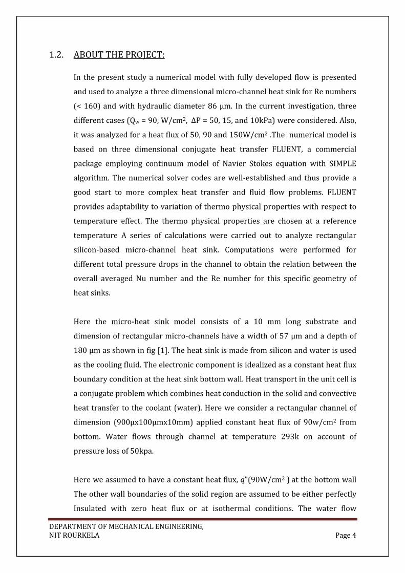
Fig. 12 Velocity contour of outlet at 30 kpa

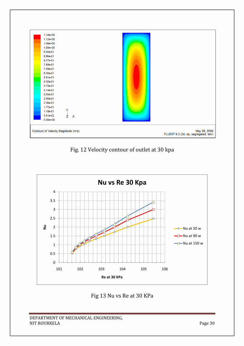
Fig 13 Nu vs Re at 30 KPa

0

0.5

1

1.5

2

2.5

3

3.5

4

101 102 103 104 105 106

Nu

Re at 30 KPa

Nu vs Re 30 Kpa

Nu at 50 w

Nu at 90 w

Nu at 150 w



Fig. 14 Combined Re vs Z

DOUBLE CHANNEL:

Fig. 15 Schematic Diagram of a Double Micro-channel in GAMBIT.

0

20

40

60

80

100

120

140

160

180

0 0.002 0.004 0.006 0.008 0.01

Re

Distance 'Z' in metres

Re vs Z

Re at 50 Kpa

Re at 30 Kpa



WATER AT 50 KPa & 50 W/cm2:

Fig. 16 Temperature of Outlet at Adiabatic wall conditions

Fig. 17 Temperature contour at Isothermal (300k) wall condition.



Fig. 18 Velocity contour at outlet (Isothermal & Adiabatic walls)

DISCUSSIONS:

GRID:

Fig 2 and Fig 15 shows the schematic diagram of Single and Double Micro-channel

respectively in GAMBIT. The modeling was done in according to the dimensions given.

The grid shows the mass flow inlet, outlet as well as the conducting walls of the heat

sink and the channels.

CONTOURS OF TEMPERATURE (SINGLE CHANNEL):

Fig 3, Fig 4 and Fig. 5 displays the filled contours of temperature at outlet of the micro-

channel for heat fluxes of 50, 90 and 150 w/cm2 at a pressure difference of 50 KPa. As

the heat flux increases, the outlet temperature goes on increasing because the fluid gets

heated up more and more due to convective heat transfer which is evident from the

contour profiles.



Fig 9, Fig 10 and Fig 11 displays the filled contours of temperature at outlet of the

micro-channel for heat fluxes of 50, 90 and 150 w/cm2 at a pressure difference of 30

KPa. As the heat flux increases, the outlet temperature goes on increasing because the

fluid gets heated up more and more due to convective heat transfer which is evident

from the contour profiles. Also, as the mass flow rate decreases, the temperature of the

outlet at a particular heat flux for 50 KPa is higher than that of 30 Kpa because less

amount of convective heat transfer takes place inside the micro-channel.

T150>T90>T50 (At 50 Kpa, 30 kPA)

T50, (50 kPA)> T50, (30 kPA)

T90, (50 kPA)> T90, (30 kPA)

T150, (50 kPA)> T150, (30 kPA)

CONTOURS OF VELOCITY (SINGLE MICRO-CHANNEL):

Fig 6 and fig 12 displays the velocity of the fluid (water) at the outlet for 50 Kpa and 30

KPa respectively. As the pressure difference decreases, the velocity decreases which is

evident from the profiles at outlet with the maximum velocity decreasing from 1.84

m/sec to 1.18 m/sec.

V50 KPa>V30 KPa

CONTOURS OF TEMPERATURE (DOUBLE MICROCHANNEL):

In case of a double Micro-channel, at 50 KPa and a heat flux of 50 w/cm2 (Fig. 16) the

outlet temperature at adiabatic wall conditions (308 k) was much greater than those at

Isothermal boundary conditions (300 k) (Fig. 17). It was also found that the outlet

temperature of double micro-channel (308 k) (Fig. 16) was lower than the single micro-

channel (309 k) (Fig. 3).

Tadiabatic, 50 KPa>Tisothermal, 50 KPa (Double Micro-channel)

Tadiabatic, double, 50 KPa< Tadiabatic, single, 50 KPa



CONTOURS OF VELOCITY (DOUBLE MICRO-CHANNEL):

The velocity of the fluid was found to be 1.62 m/sec at the outlet for a pressure

difference of 50 Kpa as shown by Fig. 18.

GRAPHS:

1. Nu vs Z Graph:

From the graph of Fig. 7, the Nusselt number at a particular heat flux keeps on

decreasing with respect to distance covered in the micro-channel. This is mainly

due to the decrease in convective heat transfer rate as the fluid gets heated up

more and more and is unable to carry that much amount of heat.

Also, it can be noticed (Fig. 7) that the nusselt number at a particular point in the

micro-channel is different for different heat fluxes and decreases with decreasing

heat flux

Nu150>Nu90>Nu50 (At 50 KPa & 30 KPa)

2. Re vs Z Graph:

Reynold’s number from the graph (Fig. 14) was found to lie in the laminar region

which proved that the value calculated was correct. It was also found that as the

pressure difference decreases from 50 KPa to 30 KPa, the Reynold’s number also

decreased with respect to distance.

Re50 KPa>Re30 KPa

3. Nu vs Re Graph:

As Reynold’s number increased, Nusselt number was also found to increase, both

in case of 50 KPa (Fig.8) and 30 KPa (Fig. 13). The slope of the graph gradually

decreased as heat flux decreased from 150 W/cm2 to 50 W/cm2. This was found

to be true in both cases of 50 KPa and also 30 KPa.



6. CONCLUSION:

The analysis performed, provides a fundamental understanding of the combined flow

and conjugate convection–conduction heat transfer in the three-dimensional micro-

channel heat sink. The model formulation is general and only a few simplifying

assumptions are made. Therefore, the results of the analysis as well as the conclusions

can be considered as quite general and applicable to any three-dimensional conjugate

heat transfer problems.

• A three-dimensional mathematical model, developed using incompressible laminar

Navier–Stokes equations of motion, is capable of predicting correctly the flow and

conjugate heat transfer in the micro-channel heat sink. It has been validated using

experimental data reported in the literature, and a good agreement has been found

between the model predictions and measurements.

• The combined convection–conduction heat transfer in the micro-channel produces

very complex three-dimensional heat flow pattern with large, longitudinal, upstream

directed heat recirculation zones in the highly conducting silicon substrate as well as

the local, transverse heat ‘vortices’ in the internal corners of the channel where the

fluid and solid are in direct contact. In the ‘vortex’ region, the local surface heat fluxes

and the local convective heat transfer coefficients (Nusselt number) become negative

because the bulk (mixed mean) temperature is not an appropriate reference

temperature for describing the heat flow direction locally everywhere. In other words,

the concept of the local heat transfer coefficient and Nusselt number is meaningless in

the strongly conjugate problems.

• Although only the right Z-wall outside the channel is heated, the heat is redistributed

by conduction within a substrate and is transferred to the coolant through all four

walls inside the channel.

• The local heat fluxes from the solid to the coolant in the small inlet region of the micro-

channel are larger than those in the further downstream portion by more than two

orders of magnitude. This is because the average convective heat transfer coefficient is

much larger in the upstream locations (the boundary layer thickness is small) and also



because the highly conducting channel walls support very effective heat redistribution

from the downstream (large convective resistance) to the upstream (small convective

resistance) regions of the channel. This finding supports the concept of the manifold

micro-channel (MMC) heat sink where the flow length is greatly reduced to small

fraction of the total length of the heat sink by using a design with multiple inter-

connected inlets and outlets.

7. APPLICATION OF MICROCHANNEL HEAT SINKS:

Theoretical analysis and experimental data strongly indicate that the forced

convection water cooled micro-channel heat sink has a superior potential for

application in thermal management of the electronic packages. The heat sink is

compact and is capable of dissipating a significant thermal load (heat fluxes of the

order 100 W/cm2) with a relatively small increase in the package temperature (less

than 20°C), if operated at the Reynolds numbers above 150.



BIBLIOGRAPHY

1. Tuckerman, D.B. and Pease, R.F.W., High-performance heat sinking for VLSI, IEEE

Electron Device Letters, 1981

2. Wu, P. and Little, W.A., Measurement of friction factors for the flow of gases in

very fine channels used for microminiature Joule-Thomson refrigerators,

Cryogenics

3. Peng, X.F., Peterson, G.P., and Wang B.X., Heat transfer characteristics of water

flowing through microchannels, Experimental Heat Transfer, 1994

4. Peng, X.F. and Peterson, G.P., Effect of thermofluid and geometrical parameters

on convection of liquids through rectangular microchannels, International

Journal of Heat and Mass Transfer, 1995, Vol. 38(4),

5. Judy, J., Maynes, D., and Webb, B.W., Characterization of frictional pressure drop

for liquid flows through microchannels, International Journal of Heat and Mass

Transfer, 2002

6. Liu, D. and Garimella, S.V., Investigation of liquid flow in microchannels, AIAA

Journal of Thermophysics and Heat Transfer, 2004, Vol. 18, p. 65–72

7. Choi, S.B., Barron, R.F., and Warrington, R.O., Fluid flow and heat transfer in

microtubes, Micromechanical Sensors, Actuators, and Systems, ASME DSC, 1991,

Vol. 32, p. 123–134

8. Rahman, m.m.and gui. Experimaental measurements of fluid flow and heat

transfer in microscale cooling passage in a chip susstrate.

9. A.G. Fedorov, R. Viskanta, Three-dimensional conjugate heat transfer in the

microchannel heat sink for electronic packaging, Int. J. Heat Mass Transfer 43 (3)

(2000)

10. FLUENT documentation.

11. Poh-Seng Lee, Suresh V. Garimella, Thermally developing flow and heat transfer

in rectangular microchannels of different aspect ratios, International Journal of

Heat and Mass Transfer 49 (2006) 3060–3067

12. www.wikipedia.com

13. Numerical Heat Transfer and Fluid Flow by Suhas V. Patankar

14. Computational fluid Dynamics by John D. Anderson.

NUMERICAL SOLUTION OF THREE DIMENSIONAL CONJUGATE HEAT...

Documents

Transcript of NUMERICAL SOLUTION OF THREE DIMENSIONAL CONJUGATE HEAT...