Conjugate Heat Transfer with Large Eddy Simulation for GasTurbine Components.

Florent Duchaine a, Simon Mendez a Franck Nicoud b, Alban Corpron c

Vincent Moureau c, Thierry Poinsot d

aCERFACS, CFD team, 42 Av Coriolis, 31057 Toulouse, FrancebApplied mathematics, University Montpellier II, France

cTurbomeca (Safran Group), Bordes, FrancedCNRS Institut de Mecanique des Fluides, Toulouse, France

Received *****; accepted after revision +++++

Presented by ......

Abstract

CHT (Conjugate heat transfer) is a main design constraint for GT (gas turbines). Most existing CHT tools aredevelopped for chained, steady phenomena. A fully parallel environnement for CHT has been developed andapplied to two configurations of interest for the design of GT. A reactive Large Eddy Simulations code and a solidconduction solver exchange data via a supervisor. A flame/wall interaction is used to assess the precision andthe order of the coupled solutions. A film-cooled turbine vane is then studied. Thermal conduction in the bladeimplies lower wall temperature than adiabatic results and CHT reproduces the experimental cooling e!ciency. Tocite this article: F. Duchaine, S. Mendez, F. Nicoud, A. Corpron, V. Moureau and T. Poinsot, C. R. Mecanique333 (2009).

Resume

Transfert de chaleur couple par simulations aux grandes echelles dans les turbines a gaz. Le transfertde chaleur couple est une contrainte forte de la conception des TAG (turbines a gaz). La plupart des outilsexistant repondent a des problemes chaines et stationnaires. Un environnement parallele pour traiter des problemesthermiques couples a ete developpe et applique a deux configurations types de la conception des TAG. Un codede simulation aux grandes echelles et un code de conduction thermique echangent des donnes via un superviseur.Une interaction flamme/paroi permet d’evaluer la precision et l’ordre des solutions couplees. L’etat thermiquestationnaire d’une aube de turbine refroidie est ensuite etudie. Le couplage thermique diminue les temperaturesadiabatiques de paroi de la pale et reproduit l’e!cacite de refroidissement experimentale. Pour citer cet article :F. Duchaine, S. Mendez, F. Nicoud, A. Corpron, V. Moureau et T. Poinsot, C. R. Mecanique 333 (2009).

Key words: Conjugate heat transfer ; Large Eddy Simulation ; Wall flame interaction ; Turbine blade

Mots-cles : Transfert de chaleur couple ; Simulation aux grandes echelles ; Interaction flamme paroi ; Aube de turbine

Preprint submitted to Elsevier Science April 9, 2009

1. Introduction

CHT (Conjugate Heat Transfer) is a key issue in combustion [1,2]: the interaction of hot gases andreacting flows with colder walls is a key phenomenon in all chambers and is actually a main designconstraint in gas turbines. For example, multi-perforated plates are commonly used in gas turbines com-bustion chambers to cool walls and they must be able to sustain the high fluxes produced in the chamber.After combustion, the interaction of the hot burnt gases with the high pressure stator and the first turbineblades conditions the temperature and pressure levels reached in the combustor, and therefore the enginee!ciency.

CHT is a di!cult field and most existing tools are developed for chained (rather than coupled), steady(rather than transient) phenomena: the fluid flow is brought to convergence using a RANS (ReynoldsAveraged Navier-Stokes) solver for a given set of skin temperatures [3,4,5]. The heat fluxes predictedby the RANS solver are then transferred to a heat transfer solver which produces a new set of skintemperatures. A few iterations are generally su!cient to reach convergence. There are circumstanceshowever where this chaining method must be replaced by a full coupling approach. Flames interactingwith walls for example, may require a simultaneous resolution of the temperature within the solid andaround it. More generally, the introduction of LES to replace RANS leads to full coupling since LESprovides the unsteady evolution of all flow variables.

Fully coupled CHT requires to take into account multiple questions. Among them, two issues wereconsidered for the present work:– The time scales of the flow and of the solid are generally very di"erent. In a gas turbine, a blade

submitted to the flow exiting from a combustion chamber has a thermal characteristic time scale of theorder of a few seconds while the flow-through time along the blade is less than 1 ms. As a consequence,the frequency of the exchanges between the codes is critical for the precision, stability and restitutiontime of the computations.

– Coupling the two phenomena must be performed on massively parallel machines where the codes mustbe not only coupled but synchronized to exploit the power of the machines.During this work, these two issues have been studied using two examples of CHT: a flame interacting

with a wall in section 3 and a blade submitted to a flow of hot gases in section 4. Both problems haveconsiderable impact on the design of combustion devices. Section 2 deals with the codes used to thisstudies as well as the coupling strategies.

2. Solvers and coupling strategies

The AVBP code is used for the fluid [6,7]. It solves the compressible reacting Navier-Stokes equationswith a third-order scheme for spatial di"erencing and a Runge Kutta time advancement [8,9]. Boundaryconditions are handled with the NSCBC formulation [10,9].

For the resolution of the heat transfer equation within solids, a simplified version of AVBP, calledAVTP, was developed. It is coupled to AVBP using the PALM software [11]. For all present examples,the skin meshes are the same for the fluid and the solid so that no interpolation error is introduced atthis level.

The coupling strategy between AVBP and AVTP depends on the objectives of the simulation and ischaracterized by two issues:

Email address: Florent.Duchaine@cerfacs.fr (Florent Duchaine).

2

Sequential coupling strategy SCS Parallel coupling strategy PCS

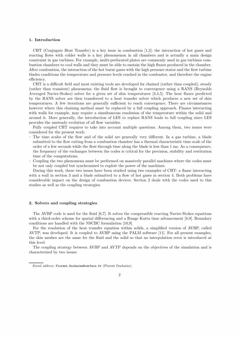
Figure 1. Main types of coupling strategies.

– Synchronization in physical time: the physical time computed by the two codes between two informationexchanges may be the same or not. We will impose that between two coupling events, the flow isadvanced in time of a quantity !f"f where "f is a flow characteristic time. Simultaneously, the solid isadvanced of a time !s"s where "s is a characteristic time for heat propagation through the solid. Twolimit cases are of interest: (1) !s = !f ensures that both solid and fluid converge to steady state at thesame rate (the two domains are then not synchronized in physical time) and (2) !f"f = !s"s ensuresthat the two solvers are synchronized in physical time.

– Synchronization in CPU time: on a parallel machine, codes for the fluid and for the structure maybe run together or sequentially. An interesting question controlled by the execution mode is the in-formation exchange. Figure 1 shows how heat fluxes and temperature are exchanged in a mode calledSCS (Sequential Coupling Strategy) where the fluid solver after run n (physical duration !f"f ) pro-vides fluxes to the solid solver which then starts and gives skin temperatures (physical duration !s"s).In SCS, the codes are loaded into the parallel machine sequentially and each solver use all availableprocessors (P ). Another solution is Parallel Coupling Strategy (PCS) where both solvers run togetherusing information obtained from the other solver at the previous coupling iteration (Fig. 1). In thiscase, the two solvers must share the P = Ps + Pf processors. The Ps and Pf processors dedicated tothe solid and the fluid respectively must be such that:

Pf

P=

1

1 + Ts/Tf(1)

where Ts and Tf are the execution times of the solid and fluid solvers respectively (on one processor)and depend on !s"s and !f"f . Perfect scaling for both solvers is assumed here.Note that both SCS and PCS questions are linked to the way information (heat fluxes and wall tem-

peratures) are exchanged and to the implementation on parallel machines but are independent of thesynchronization in physical time: PCS or SCS can be used for steady or unsteady computations. Thispaper focuses on the PCS.

Finally, this work explores the simplest coupling method where the fluid solver provides heat fluxes tothe solid solver while the solid solver sends skin temperatures back to the fluid code. More sophisticatedmethods may be used for precision and stability [12,13] but the present one was found su!cient for thetwo test cases described below.

3

Figure 2. Interaction between wall and premixed flame. Solid line: initial temperature profile.

Figure 3. The IFF (infinitely fast flame) limit. Solid line: initial temperature profile.

3. Flame/wall interaction (FWI)

The interaction between flames and walls controls combustion, pollution and wall heat fluxes in asignificant manner [10,14,15]. It also determines the wall temperature and its life time. In most combustiondevices, burnt gases reach temperatures between 1500 and 2500 K while walls temperatures remainbetween 400 and 850 K because of cooling. The temperature decrease from burnt gases levels to walllevels occurs in a near-wall layer which is less than 1 mm thick, creating large temperature gradients.

Studying the interaction between flames and walls is di!cult from an experimental point of viewbecause all interesting phenomena occur in a thin zone near the wall: in most cases, the only measurablequantity is the unsteady heat flux through the wall. Moreover, flames approaching walls are dominatedby transient e"ects: they usually do not ’touch’ walls and quench a few micrometers away from the coldwall because the low wall temperature inhibits chemical reactions. At the same time, the large near-walltemperature gradients lead to very high wall heat fluxes. These fluxes are maintained for short durationsand their characterization is also a di!cult task in experiments [16,17].

The present study focuses on the interaction between a laminar flame and a wall (Fig. 2). Except for afew studies using integral methods within the solid [18] or catalytic walls [19,20], most studies dedicatedto FWI were performed assuming an inert wall at constant wall temperature. Here we will revisit theassumption of isothermicity of the wall during the interaction.

3.1. The Infinitely Fast Flame (IFF) limit

Flame front thicknesses (#oL) are less than 1 mm and laminar flame speeds (so

L) are of the order of 1 m/s.Walls are usually made of metal or ceramics and their characteristic time scale "s = L2/Ds (where L is thewall thickness and Ds the wall di"usivity) is much longer than the flame characteristic time " = #o

L/soL.

An interesting simplification of this observation is the ’Infinitely Fast Flame’ limit (IFF) in which thetime scale of the flame is assumed to be zero compared to the solid time. In this case, the FWI limitcan be replaced by the simpler case of a semi-infinite solid at temperature T1 getting instantaneously intouch with a semi-infinite fluid at a constant temperature T2 where T2 is the adiabatic flame temperature(Fig. 3). The propagation time of the flame towards the wall is neglected.

The IFF problem is a classical heat transfer problem and has an analytical solution which can bewritten as:

T (x, t) = T1 + bT2 ! T1

b + bserfc(!

x

2"

Dst) for x < 0 (2)

T (x, t) = T2 ! bsT2 ! T1

b + bserfc(

x

2"

Dt) for x > 0 (3)

4

Initial Thermal Thermal Thermal Heat Density Mesh Fourier

temperature di!usivity e!usivity conductivity capacity size time step

Solid 650 3.38 10!6 7058.17 12.97 460 8350 4 10!6 2.37 10!6

Fluid 660 2.53 10!5 5.52 0.028 1162.2 0.947 4 10!6 3.16 10!7

Table 1Fluid and solid characteristics for IFF test case (SI units). The Fourier time step corresponds to the stability limit forexplicit schemes "tD = "x2/(2Dth).

where b =!

$%Cp is the e"usivity of the burnt gases, bs =!

$s%sCps the e"usivity of the wall andD the burnt gases di"usivity . Ds and D are assumed to be constant in the solid and fluid parts. Thetemperature of the wall at x = 0 is constant and the heat flux # decreases like 1/

"t:

T (x = 0, t) =bT2 + bsT1

b + bsand #(x = 0, t) =

T2 ! T1

b + bs

bbs"&t

(4)

This IFF limit is useful to understand FWI limits. It was also used as a test case of the coupled codesto check the accuracy of coupling strategies (next section).

3.2. The IFF limit as a test case for unsteady fluid / heat transfer coupling

A central question for SCS or PCS is the coupling frequency between the two solvers especially whenthey have very di"erent characteristic times. Since the IFF has an analytical solution, it was first usedas a test case for PCS. The test case corresponds to a wall at 650 K in contact at t = 0 with a fluidat 660 K. Compared to a wall/flame interaction, this small temperature di"erence is chosen in order tokeep constant values for D, $ and Cp. Table 1 summarizes the properties of the solid and the fluid andindicates mesh size $x and maximum time steps $tD for di"usion.

The most interesting part of this problem is the initial phase when fluxes are large and coupling di!cult.During this phase, the solid and the fluid can be considered as infinite and there is no proper length ortime scale to evaluate "f or "s in Fig. 1. The only useful scale is the grid mesh and the associated timescale for explicit algorithm stability. Therefore we chose to take "f = $tDf and "s = $tDs (Note that

the fluid solver is limited by an acoustic time step smaller than $tDf ). The strategy used for this test isthe PCS (Fig. 1) for unsteady cases which requires !f"f = !s"s . The !f parameter defines the timeinterval between two coupling events normalized by the fluid characteristic time. Values of !f rangingfrom 0.131 to 65.5 were tested for this problem and Fig. 4 shows how the errors on maximum walltemperature and the wall heat flux change when !f changes. The IFF solution (Eq. 4) is used as thereference solution. Using values of !f larger than unity leads to relative errors which can be significantand to strong oscillations on the temperature and flux. As expected a full coupling of fluid and solid forthis problem requires to use values of !f of order unity which means to couple the codes on a time scalewhich is of the order of the smallest time scale (here the flow time scale).

3.3. Flame/wall interaction results

This section presents results obtained for a fully coupled FWI and compares them to the IFF limit.The parameters used for the simulation (Table 2) correspond to a methane/air flame at an equivalenceratio of 0.8, propagating in fresh gases at a temperature T1 of 650 K at a laminar speed so

L = 1.128 m/s.The adiabatic flame temperature is T2 = 2300 K. The wall is initially at T1 = 650 K . The maximum timestep corresponds to the Fourier stability criterion for the solid ($tFs = 0.59 µs) and to the CFL stabilitycriterion for the fluid ($tCFL

f = 0.0023 µs). For this fully coupled problem, the only free parameter is !f .

5

0 100 200 300 400

-1e-05

-5e-06

0e+00

5e-06

Reduced time t+ = t/"fRel

ativ

eer

ror

onte

mper

ature

0 100 200 300 400-1

-0.5

0

0.5

1

1.5

Reduced time t+ = t/"f

Rel

ativ

eer

ror

onflux

Figure 4. Tests of the PCS for the IFF case of Fig. 3. E!ects of the coupling period between two events (measured by !s).Left: relative error on wall temperature at x = 0, right: relative error on wall flux at x = 0. Solid line: !f = 0.131, dashed:!f = 13.1, dots: !f = 65.5.

Initial Thermal Thermal Thermal Heat Density Mesh Time

temperature di!usivity e!usivity conductivity capacity size scale

Solid 650 3.38 10!6 7058.17 12.97 460 8350 2 10!6 0.3

Fresh gases 650 4.14 10!5 7.35 0.047 1168.9 0.977 4 10!6 30.45 10!6

Hot gases 2300 3.72 10!4 7.28 0.140 1441.6 0.262 4 10!6 30.45 10!6

Table 2Fluid and solid characteristics for flame/wall interaction test case (SI units). The characteristic time "s for the solid is basedon its thickness and heat di!usivity. The characteristic time scale for the fluid "f is based on the flame speed and thickness.

The period between two coupling events (!f"f = !s"s) determines the number of iterations performed bythe gas solver during this time: Nit = !f"f/$tCFL

f . As the cost of computing heat transfer in the solidfor this problem is actually negligible, no attempt was made to optimize the computation. The e"ect ofmesh resolution in the gases was also checked and found to be negligible: for most runs, 500 mesh pointsare used in the gases with a mesh size of 4 10!6 mm.

The coupling parameters for the presented case correspond to a PCS simulation with !f = 7.5 10!3

leading to Nit = 100 in the gases accompanied by one iteration in the solid where !s = 7.6 10!7

(Fig. 5). Figure 6 displays the wall scaled temperature at the fluid and solid interface T " = (T (x =0) ! T1)/(T2 ! T1)) and the reduced maximum heat flux #/(%Cpso

L(T2 ! T1)) through the wall versustime. The flame quenches at time so

Lt/#oL = 9, where the flux is maximum. Figure 6 also displays the

prediction of the IFF limit (Eq. 4). Except in the first instants of the interaction, when the flame isstill active, the IFF limit matches the simulation results extremely well, both in terms of fluxes and walltemperature. The IFF solution can not predict the maximum heat flux because it leads to an infinite fluxat the initial time. However, as soon as the flame is quenched, it gives a very good evaluation of the wallheat flux. Note that the wall temperature increases by a small amount during this interaction betweenan isolated flame and the wall (T " # 10!3 on Fig. 6). In more realistic cases, flame will flop and hit wallsat high frequency which could lead to cumulative e"ects and therefore to higher wall temperature andfatigue.

Fig. 7 shows how the wall temperature at x = 0 changes when the e"usivity of the solid varies. Forthe IFF limit, this temperature is given by Eq. 4 and for the simulation, it is the temperature reachedasymptotically for long times. The agreement is excellent and confirms that the IFF limit correctly predictsthe long-term evolution in this FWI problem. It also shows that the coupled simulation works correctly.Note however, that the IFF limit given by Eq. 4 is only approximate for the flame wall interaction problem

6

Figure 5. Parallel coupling strategy for the flame/wall interaction with !f = 7.5 10!3.

0 20 40 60 800.0e+00

2.5e-04

5.0e-04

7.5e-04

1.0e-03

Reduced time t+ = #oLt/so

L

Red

uce

dte

mper

ature

0 20 40 60 800

0.1

0.2

0.3

0.4

Reduced time t+ = #oLt/so

L

Red

uce

dhea

tflux

Figure 6. Coupled flame/wall interaction simulation (solid line). Comparison with IFF limit adjusted to start at flamequenching (dashed line). Left: reduced wall temperature (x = 0), right: reduced wall heat flux at x = 0.

100 1000 10000 1e+05 1e+060

0.005

0.01

0.015

0.02

0.025

0.03

Wall e"usivity

Red

uce

dte

mper

ature

Figure 7. Coupled flame/wall interaction simulation. Reduced wall temperature (T (x = 0)!T1)/(T2 !T1)) vs wall e!usivitybs. Solid line: IFF limit, circles: coupled simulation.

since it assumes constant density and heat di"usivity in the gases.Finally, Fig. 8 shows how the coupling frequency (measured by the parameter !f ) changes the precision

of the coupled simulation (coupling events are scheduled at every !f"f times where "f is the fluid time).The precision of the coupling was checked by changing Nit from 100 to 500000 (!f from 7.5 10!3 to 37.8)with Nit = 10 (!f = 7.5 10!4) as reference. The error on the maximum temperature remains very smalleven for large !f values. The error on the maximum energy entering the wall between the initial timeand an arbitrary instant (here #o

Lt/soL = 82) depends strongly on !f . As expected from results obtained

for the IFF problem only (previous section), coupling the two solvers less often that "f (!f > 1) leads toerrors larger than 10 percent on the energy fluxed into the wall. The errors on temperature and energyfluxed into the wall converge both to 0 when !f decreases with an order close to 1.

7

0.01 0.1 1 10

1e-06

1e-05

0.0001

0.001

First Order

!f

Rel

ativ

eer

ror

onw

allte

mper

ature

0.01 0.1 1 10

0.01

0.1

1

First

Order

!f

Rel

ativ

eer

ror

onen

ergy

Figure 8. Flame/wall interaction simulation. Left: relative error on wall temperature (x = 0) from t+ = #oLt/so

L = 0 tot+ = 82, right: relative error on the energy fluxed into the wall on the same period.

4. Blade cooling

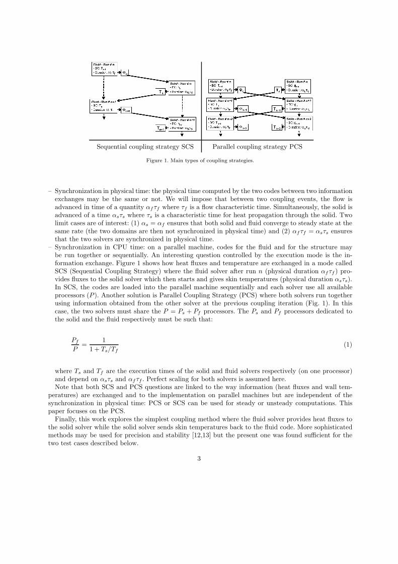
The second application is the interaction between a high-speed flow and a cooled blade. This exampleis typical of the main problems encountered during the design of combustion chambers [2,21]: the hot flowleaving the combustor must not burn the turbine blades or the vanes of the high pressure stator. Predictingthe vanes temperature field (which are cooled from the inside by cold air) is a major research area [22,23,4].Here an experimental set-up (T120D blade, Fig. 9) developed within the AITEB-1 European projectwas used to evaluate the precision of the coupled simulations. The temperature di"erence between themainstream (T2 = 333.15K) and cooling (T1 = 303.15K) airs is limited to 30 K to facilitate measurements.Experimental results include pressure data on the blade suction and pressure sides as well as temperaturemeasurement on the pressure side.

The computational domains for both fluid and structure contain only one spanwise pitch of the filmcooling hole pattern (z axis on Fig. 9), with periodicity enforced at each end. A periodicity condition isalso assumed in the y direction. 6.5 million cells are used to discretize the fluid and 600 000 for the solid.The WALE subgrid model [24] is used in conjunction with no-slip wall conditions. The three film-coolingholes and the plenum are included in the domain (Fig. 9): jet 2 is aligned with the main flow (in the xyplane) while jets 1 and 3 have a compound orientation. The mean blowing ratio (ratio of a jet momentumon the hot flow momentum) of the jets is approximately 2.5.

Tables 3 and 4 summarize the properties of the gases and of the solid used for the simulation. At eachcoupling event, fluxes and temperature on the blade skin are exchanged as described in Fig. 1. Duringthis work, only a steady state solution within the solid was sought so that time consistency was notensured during the coupling computation (!f = !s). The converged state is obtained with a two stepmethodology which consists in:

(i) Initialization of the coupled calculation including a thermal converged adiabatic fluid simulationand a thermal converged isothermal solid computation with boundary temperatures given by thefluid solution,

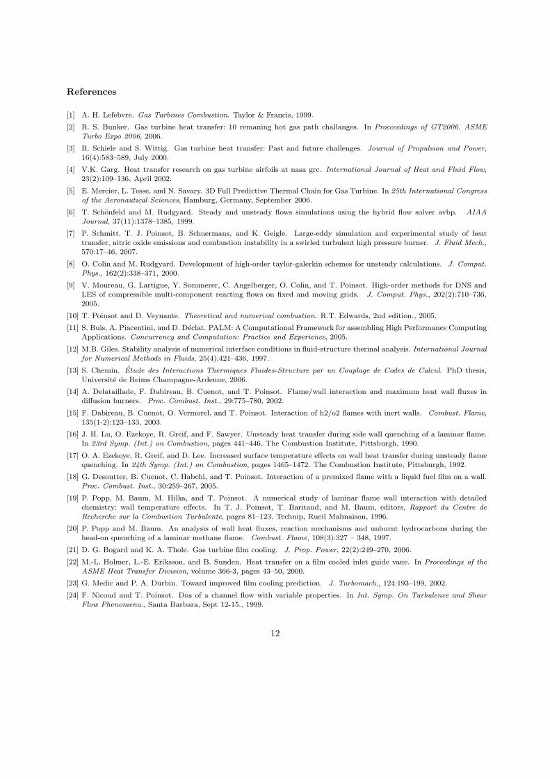
(ii) Coupled simulation.Convergence is investigated by plotting the history of the total flux on the blade (which must go to zero)

and of the minimum and maximum blade temperatures. Figures 10 show these results for two variants ofthe PCS. In the first one, fluxes and temperature are exchanged at each coupling step while for the secondone, relaxation is used and temperature and fluxes imposed at each coupling iteration n are written asfn = afn!1 + (1 ! a)fn" where fn" is the value obtained by the other solver at iteration n and a is arelaxation factor (typically a = 0.6). Without relaxation, the choice of a unique value of ! for the fluid

8

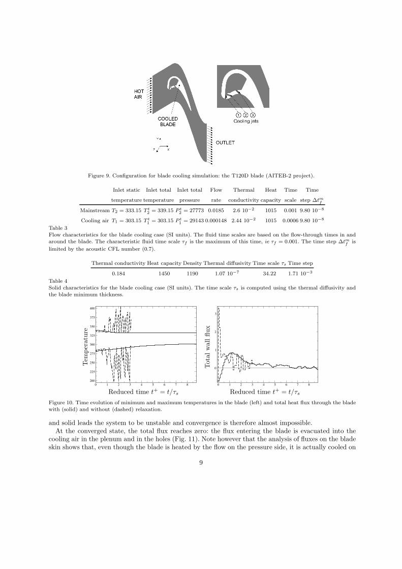
Figure 9. Configuration for blade cooling simulation: the T120D blade (AITEB-2 project).

Inlet static Inlet total Inlet total Flow Thermal Heat Time Time

temperature temperature pressure rate conductivity capacity scale step "tmf

Mainstream T2 = 333.15 T t2 = 339.15 P t

2 = 27773 0.0185 2.6 10!2 1015 0.001 9.80 10!8

Cooling air T1 = 303.15 T t1 = 303.15 P t

1 = 29143 0.000148 2.44 10!2 1015 0.0006 9.80 10!8

Table 3Flow characteristics for the blade cooling case (SI units). The fluid time scales are based on the flow-through times in andaround the blade. The characteristic fluid time scale "f is the maximum of this time, ie "f = 0.001. The time step "tmf is

limited by the acoustic CFL number (0.7).

Thermal conductivity Heat capacity Density Thermal di!usivity Time scale "s Time step

0.184 1450 1190 1.07 10!7 34.22 1.71 10!3

Table 4Solid characteristics for the blade cooling case (SI units). The time scale "s is computed using the thermal di!usivity andthe blade minimum thickness.

0 1 2 3 4 5 6 7 8200

225

250

275

300

325

350

375

400

Reduced time t+ = t/"s

Tem

per

ature

0 1 2 3 4 5 6 7 8

0

1

2

3

Reduced time t+ = t/"s

Tot

alw

allflux

Figure 10. Time evolution of minimum and maximum temperatures in the blade (left) and total heat flux through the bladewith (solid) and without (dashed) relaxation.

and solid leads the system to be unstable and convergence is therefore almost impossible.At the converged state, the total flux reaches zero: the flux entering the blade is evacuated into the

cooling air in the plenum and in the holes (Fig. 11). Note however that the analysis of fluxes on the bladeskin shows that, even though the blade is heated by the flow on the pressure side, it is actually cooled on

9

0 5 10 15 20 25 30

-0.8

-0.6

-0.4

-0.2

0

0.2

0.4

0.6

0.8

Reduced time t+ = t/"s

Hea

tfluxe

s

0 0.2 0.4 0.6 0.8 10

0.2

0.4

0.6

0.8

1

Reduced abscissa

Isen

trop

icM

ach

num

ber

Mis

Figure 11. Time evolution of heat fluxes through the blade (left): external flux (solid line), plenum (dashed), holes sides(dot), sum of all fluxes (dot dashed). Isentropic Mach number along the blade (right): coupled LES (solid line), adiabaticLES (circles), experiment (squares).

part of the suction side because the flow accelerates and cools down on this side. Due to the accelerationin the jets, heat transfer in the holes and plenum are of the same order. Compared to the external flux,plenum and hole fluxes converge almost linearly. Oscillations in the external flux evolution are linked withthe complex flow structure developing around the blade.

At the converged state, results can be compared to the experiment in terms of pressure profiles on theblade (on both sides) and of temperature profiles on the pressure side. Pressure fields are displayed interms of isentropic Mach numbers Mis computed by

Mis =

"

#

#

$

2

' ! 1

%

&

P t2

P tw

'

!!1

!

! 1

(

(5)

where P t2 and P t

w are the total pressure of the main stream and at the wall. Figure 11 displays anaverage field of isentropic Mach number obtained by LES and by the experiment. The comparison ofthe adiabatic simulation and the coupled one shows that these profiles are only weakly sensitive to thethermal condition imposed on the blade. Although the shock position on the suction side is not perfectlycaptured, the overall agreement between LES and experimental results is fair.

Temperature results are displayed in terms of cooling e!ciency % = (T t2 ! T )/(T t

2 ! T t1) where T t

2

and T t1 are the total temperatures of the main and cooling streams (Table 4) and T is the local wall

temperature. Figure 12 shows measurements, adiabatic and coupled LES results for % spanwise averagedalong axis x. As expected, the cooling e!ciency obtained with the adiabatic computation are lower thanthe experimental values: the adiabatic temperature field over-predicts the real one. The main contributionof conduction in the blade is to reduce the wall temperature on the pressure side.

The reduced temperature distribution on the pressure side (Fig. 13) shows that the peak temperatureoccurs at the stagnation point (reduced abscissa close to 0). The temperature at the stagnation point isreduced compared to the adiabatic wall prediction, leading to local values of ( of the order of 0.2. Thethermal e"ects of the cooling jets on the vane are clearly evidenced by Fig. 13. Jet 3 seems to be themost active in the cooling process by protecting the blade from the hot stream until a reduced absissa of0.5 and then impacting the vane between 0.5 and 0.6.

The reduced temperature obtained during this work over estimates experimental measurements. Inparticular, the strong acceleration caused by the blade induce large thermal gradients at the trailingedge. This phenomenon not well resolved by the computations leads to a non physical values of coolinge!ciency. Nevertheless, these results have shown a very large sensitivity to multiple parameters, not only

10

0 0.2 0.4 0.6 0.8 10

0.2

0.4

0.6

Reduced abscissa

Coo

ling

e!ci

ency

Figure 12. Cooling e#ciency $ versus abscissa on the pressure side at steady state. Dashed line: adiabatic LES, solid line:coupled LES, symbols: experiment from UNIBW, vertical dashed lines: position of the holes.

Figure 13. Spatial distribution of reduced temperature $ on the pressure side of the blade. The computational domain isduplicated one time in the z direction.

of the coupling strategy but also of the LES models for heat transfer and wall descriptions.

5. Conclusions

CHT calculations have been performed for two configurations of importance for the design of gas tur-bines with a recently developed massively parallel tool based on a LES solver. (1) An unsteady flame/wallinteraction problem was used to assess the precision of coupled solutions when varying the coupling pe-riod. It was shown that the maximum coupling period that allows to well reproduce the temperature andthe flux across the wall is of the order of the smallest time scale of the problem. (2) Steady convective heattransfer computation of an experimental film-cooled turbine vane showed how thermal conduction in theblade tend to reduce wall temperature compared to an adiabatic case. Further studies on LES models,coupling strategy and experimental conditions are needed to improve quality of the results compared tothe experimental cooling e!ciency.

Acknowledgements

This work was done during the Summer Program of CTR 2008. The help of L. Pons from TURBOMECAand of the AITEB-1 and AITEB-2 consortium for the experimental results is gratefully acknowledged.

11

References

[1] A. H. Lefebvre. Gas Turbines Combustion. Taylor & Francis, 1999.

[2] R. S. Bunker. Gas turbine heat transfer: 10 remaning hot gas path challanges. In Procceedings of GT2006. ASMETurbo Expo 2006, 2006.

[3] R. Schiele and S. Wittig. Gas turbine heat transfer: Past and future challenges. Journal of Propulsion and Power,16(4):583–589, July 2000.

[4] V.K. Garg. Heat transfer research on gas turbine airfoils at nasa grc. International Journal of Heat and Fluid Flow,23(2):109–136, April 2002.

[5] E. Mercier, L. Tesse, and N. Savary. 3D Full Predictive Thermal Chain for Gas Turbine. In 25th International Congressof the Aeronautical Sciences, Hamburg, Germany, September 2006.

[6] T. Schonfeld and M. Rudgyard. Steady and unsteady flows simulations using the hybrid flow solver avbp. AIAAJournal, 37(11):1378–1385, 1999.

[7] P. Schmitt, T. J. Poinsot, B. Schuermans, and K. Geigle. Large-eddy simulation and experimental study of heattransfer, nitric oxide emissions and combustion instability in a swirled turbulent high pressure burner. J. Fluid Mech.,570:17–46, 2007.

[8] O. Colin and M. Rudgyard. Development of high-order taylor-galerkin schemes for unsteady calculations. J. Comput.Phys., 162(2):338–371, 2000.

[9] V. Moureau, G. Lartigue, Y. Sommerer, C. Angelberger, O. Colin, and T. Poinsot. High-order methods for DNS andLES of compressible multi-component reacting flows on fixed and moving grids. J. Comput. Phys., 202(2):710–736,2005.

[10] T. Poinsot and D. Veynante. Theoretical and numerical combustion. R.T. Edwards, 2nd edition., 2005.

[11] S. Buis, A. Piacentini, and D. Declat. PALM: A Computational Framework for assembling High Performance ComputingApplications. Concurrency and Computation: Practice and Experience, 2005.

[12] M.B. Giles. Stability analysis of numerical interface conditions in fluid-structure thermal analysis. International Journalfor Numerical Methods in Fluids, 25(4):421–436, 1997.

[13] S. Chemin. Etude des Interactions Thermiques Fluides-Structure par un Couplage de Codes de Calcul. PhD thesis,Universite de Reims Champagne-Ardenne, 2006.

[14] A. Delataillade, F. Dabireau, B. Cuenot, and T. Poinsot. Flame/wall interaction and maximum heat wall fluxes indi!usion burners. Proc. Combust. Inst., 29:775–780, 2002.

[15] F. Dabireau, B. Cuenot, O. Vermorel, and T. Poinsot. Interaction of h2/o2 flames with inert walls. Combust. Flame,135(1-2):123–133, 2003.

[16] J. H. Lu, O. Ezekoye, R. Greif, and F. Sawyer. Unsteady heat transfer during side wall quenching of a laminar flame.In 23rd Symp. (Int.) on Combustion, pages 441–446. The Combustion Institute, Pittsburgh, 1990.

[17] O. A. Ezekoye, R. Greif, and D. Lee. Increased surface temperature e!ects on wall heat transfer during unsteady flamequenching. In 24th Symp. (Int.) on Combustion, pages 1465–1472. The Combustion Institute, Pittsburgh, 1992.

[18] G. Desoutter, B. Cuenot, C. Habchi, and T. Poinsot. Interaction of a premixed flame with a liquid fuel film on a wall.Proc. Combust. Inst., 30:259–267, 2005.

[19] P. Popp, M. Baum, M. Hilka, and T. Poinsot. A numerical study of laminar flame wall interaction with detailedchemistry: wall temperature e!ects. In T. J. Poinsot, T. Baritaud, and M. Baum, editors, Rapport du Centre deRecherche sur la Combustion Turbulente, pages 81–123. Technip, Rueil Malmaison, 1996.

[20] P. Popp and M. Baum. An analysis of wall heat fluxes, reaction mechanisms and unburnt hydrocarbons during thehead-on quenching of a laminar methane flame. Combust. Flame, 108(3):327 – 348, 1997.

[21] D. G. Bogard and K. A. Thole. Gas turbine film cooling. J. Prop. Power, 22(2):249–270, 2006.

[22] M.-L. Holmer, L.-E. Eriksson, and B. Sunden. Heat transfer on a film cooled inlet guide vane. In Proceedings of theASME Heat Transfer Division, volume 366-3, pages 43–50, 2000.

[23] G. Medic and P. A. Durbin. Toward improved film cooling prediction. J. Turbomach., 124:193–199, 2002.

[24] F. Nicoud and T. Poinsot. Dns of a channel flow with variable properties. In Int. Symp. On Turbulence and ShearFlow Phenomena., Santa Barbara, Sept 12-15., 1999.

12