
3D Conjugate Heat Transfer Simulation of Aircraft...
116
3D Conjugate Heat Transfer Simulation of Aircraft Hot-Air Anti-Icing Systems Hong Zhi Wang Department of Mechanical Engineering McGill University Montreal, Québec September 2005 A Thesis Submitted to McGill University in Partial Fulfillment of the Requirements of the Degree of Master of Engineering © Hong Zhi Wang, 2005
Transcript of 3D Conjugate Heat Transfer Simulation of Aircraft...

3D Conjugate Heat Transfer Simulation of
Aircraft Hot-Air Anti-Icing Systems
Hong Zhi Wang
Department of Mechanical Engineering
McGill University
Montreal, Québec
September 2005
A Thesis Submitted to McGill University in
Partial Fulfillment of the Requirements of the Degree of Master of Engineering
© Hong Zhi Wang, 2005
1+1 Library and Archives Canada
Bibliothèque et Archives Canada
Published Heritage Branch
Direction du Patrimoine de l'édition
395 Wellington Street Ottawa ON K1A ON4 Canada
395, rue Wellington Ottawa ON K1A ON4 Canada
NOTICE: The author has granted a nonexclusive license allowing Library and Archives Canada to reproduce, publish, archive, preserve, conserve, communicate to the public by telecommunication or on the Internet, loan, distribute and sell th es es worldwide, for commercial or noncommercial purposes, in microform, paper, electronic and/or any other formats.
The author retains copyright ownership and moral rights in this thesis. Neither the thesis nor substantial extracts from it may be printed or otherwise reproduced without the author's permission.
ln compliance with the Canadian Privacy Act some supporting forms may have been removed from this thesis.
While these forms may be included in the document page count, their removal does not represent any loss of content from the thesis.
• •• Canada
AVIS:
Your file Votre référence ISBN: 978-0-494-22681-0 Our file Notre référence ISBN: 978-0-494-22681-0
L'auteur a accordé une licence non exclusive permettant à la Bibliothèque et Archives Canada de reproduire, publier, archiver, sauvegarder, conserver, transmettre au public par télécommunication ou par l'Internet, prêter, distribuer et vendre des thèses partout dans le monde, à des fins commerciales ou autres, sur support microforme, papier, électronique et/ou autres formats.
L'auteur conserve la propriété du droit d'auteur et des droits moraux qui protège cette thèse. Ni la thèse ni des extraits substantiels de celle-ci ne doivent être imprimés ou autrement reproduits sans son autorisation.
Conformément à la loi canadienne sur la protection de la vie privée, quelques formulaires secondaires ont été enlevés de cette thèse.
Bien que ces formulaires aient inclus dans la pagination, il n'y aura aucun contenu manquant.

Acknowledgments
First of aIl, I would like to express my great appreciation of my Professor, Dr. Wagdi
Habashi who opened the do or and led me into the marvelous world of CFD. I benefited
from his superb academic attainments and outstanding leadership, not only in scientific
research but also in philosophy of life during the course of my study at the CFD Lab.
I would like to thank the NSBRC-J. Armand Bombardier Industrial Research Chair of
Multidisciplinary CFD, whose financial support made my research possible.
I would also like to express my deep gratitude to my thesis co-supervisor, Dr. François
Morency, currently a professor at BTS. He helped me during the entire course of my
research and taught me a lot about icing and anti-icing simulation, with excellent and
patient guidance. Moreover, many thanks are due to Professor Héloïse Beaugendre of
Bordeaux University, my colleague at the beginning of my research, who shared a
detailed knowledge of aero-icing simulation with me and instructed me in the hands-on
experience to use different CFD tools.
I am also grateful to Dr. Frédéric Tremblay, Dr. Claude Lepage, and Martin Aubé at
Newmerical Technologies International (NTI) for their valuable advices and sincere help
in my research. My thanks also go to Dr. Croce of the University of Udine, a long-term
associate of the CFD lab, for his advice and help in Conjugate Heat Transfer.
My colleges at the CFD Lab have given me continuous help and support in both my
studies and my life. They have made my intensive Master study full of pleasure and
beautiful memories. Because of them, I more and more love this peaceful country, my
second motherland. 1 would like to give my special thanks to my buddies Raimund
Honsek, Nabil Ben Abdallah, France Suerich-Gulick, Peter Findlay, Farid Kachra,
LiangKan Zheng ...

l also wish to thank Laboratoire de Mécanique des Fluides (LMF) of Laval University for
providing the anti-icing experiment conducted in 2003 by Jean Lemay, Yvan Maciel et al.
l would like to dedicate this thesis to my parents who have always loved and supported
me unconditionally throughout my whole life. Aiso to be thanked are my best friends.
They are the most important people in my life and love me as a member of their family.
ii
Abstract
When an aircraft flies through clouds under icy conditions, supercooled water droplets at
temperatures below the freezing point may impact on its surfaces and result in ice
accretion. The design of efficient devices to protect aircraft against in-flight icing
continues to be a challenging task in the aerospace industry. Advanced numerical tools to
simulate complex conjugate heat transfer phenomena associated with hot-air anti-icing
are needed. In this work, a 3D conjugate heat transfer procedure based on a 100 se
coupling method has been developed to solve the following four domains: the external
airflow, the water film, conduction in the solid, and the internaI airflow. The domains are
solved sequentially and iteratively, with an exchange of thermal conditions at common
interfaces until equilibrium of the entire system is achieved. A verification test case
shows the capability of the approach in simulating a variety of anti-icing and de-icing
cases: fully evaporative, running wet, or iced. The approach is validated against a 2D dry
air experimental test case, because of the dearth of appropriate open literature 3D test data.
iii

Résumé
Quand un avion vole à travers les nuages à des conditions glaciales, de la glace risque de
se former sur ses surfaces en raison de 1'impact des gouttelettes d'eau surfondues. La
conception d'efficaces dispositifs qui protégerait 1'avion contre cette formation de glace
s'avère une tache ardue et défiante pour 1'industrie aérospatiale. Des outils numériques
simulant le transfert de chaleur conjugué associé au antigivrage par air chaud constituent
un premier choix. Ce papier présente une méthode tridimensionnelle de transfert de
chaleur conjugué, qui résout les quatre domaines suivants: 1'écoulement d'air extérieur, le
film d'eau, la conduction dans le solide ainsi que 1'écoulement d'air interne. Les domaines
sont résolus séquentiellement et itérativement, avec un échange de conditions frontières
thermales au niveau des interfaces communes, jusqu'à 1'établissement d'un équilibre
global. Un cas test de vérification montre les capacités de 1'approche dans la simulation
d'une variété de situations d'antigivrage et dégivrage : évaporation totale, écoulement
liquide ou glace. L'approche est ensuite validée à travers une comparaison
bidimensionnelle avec un cas test expérimental. Le choix bidimensionnel est dicté par la
rareté de cas tests tridimensionnels disponibles dans la littérature.
iv
Acknowledgments
Abstract
Résumé
Table of Contents
List of Symbols
List of Figures
List of Tables
Table of Contents
CHAPTER 1: Introduction
1.1 In-flight Icing Phenomena
1.2
1.3
In-flight Icing Protection and Aircraft AntilDe-Icing Systems
CFD Toois for In-:flight Icing and Anti/De-Icing Analysis
1.4 Objective of Current Work
CHAPTER 2: Literature Jl,eview
2.1 Methodology of Conjugate Heat Transfer Calculation
2.1.1 Empirical Method for Heat Transfer Problems
2.1.2 Conjugate Method for Heat Transfer Problems
2.1.2.1 Tight-Coupling Approach
2.1.2.2 Loose-Coupling Approach
i
iii
iv
v
viii
xiv
xvii
1
1
2
5
7
9
9
9
11
11
13
2.2 Overview of Numerical Simulations for Aircraft Hot-Air Anti-Icing Systems 16
2.2.1 Hot-Air Anti-Icing Simulation in LEWICE 17
2.2.2 Hot-Air Anti-Icing Simulation in CHT2D 20
2.3 Introduction of A Simplified Anti-Icing Experiment 22
2.4
2.5
Review of Heat Transfer for A Single Slot Jet Impingement
Conclusions
CHAPTER 3: Mathematical Equations and Numerical Methods
3.1 Airflow Model (FENSAP)
3.1.1 Goveming Equations
3.1.2 Numerical Discretization
3.1.3 Turbulence Models
24
26
27
27
27
29
31
v
3.1.3.1 Spalart-Allmaras Turbulence Model
3.1.3.2 k-e Turbulence Model
3.1.4 Rough Walls Prédiction in Spalart-Allmaras Model
3.1.5 Convective Heat Flux
3.2 Droplets Impingement Model (DROP3D)
3.3 WaterFilmlICE Accretion Thermodynamic Model (lCE3D)
3.4 Heat Conduction Model (C3D)
CHAPTER 4: Aigorithm for Hot-Air Anti-lcing Simulation
4.1 General Introduction of Hot-Air Anti-Icing Simulation
4.2 Overall Energy Balance in the Hot-Air Anti-Icing System
4.3 Methodology of Hot-Air Anti-Icing Simulation
4.4 Algorithm of CHT3D Hot-Air Anti-Icing Model
4.4.1 Thermal Boundary Conditions for Each Solver
4.4.2 Flow Chart of CHT3D Algorithm
4.4.3 Boundary Condition Exchange at Each Interface
4.4.4 Implementation of Hot-Air Anti-Icing Simulation in CHT3D
. 4.4.5 Dual Surface Meshes
4.4.6 Boundary Condition Exchange for Matching and Non-Matching Grids
32
33
34
35
36
39
43
44
44
46
48
49
49
51
52
54
56
57
4.4.7 The Stability Analysis of Conjugate Heat Transfer Anti-Icing Simulation 60
4.5 Conclusions 61
CHAPTER 5: Testing of CHT3D Code 62
5.1 Description of a 2-D Verification Hot-Air Anti-icing Test Case 62
5.2 Hot-Air Anti-Icing Simulations 63
5.2.1 Case 1: Hot-Air Anti-Icing Simulation with Ice Accretion 63
5.2.2 Case 2: Hot-Air Anti-Icing Simulation with Running Wet 65
5.2.3 Case 3: Hot-Air Anti-Icing Simulation with Full Evaporation 66
5.2.4 Case 4: Hot-Air Anti-Icing Simulation Without Droplets Impingement 67
5.3 Conclusion 68
CHAPTER 6: Validation of CHT3D Code 69
6.1 Validation of Turbulence Models in FENSAP for Impinging Slot Jet 69
6.1.1 Description oflmpinging Slot Jet Experiment 69
VI
6.1.2 Numerical Implementation with Spalart-Allmaras Turbulence Model 72
6.1.3 Numerical Implementation with k-s Turbulence Model 74
6.1.4 Comparison and Conclusion of Impinging Slot Jet Simulations 75
6.2 Validation of CHT3D Code with a Simplified Hot-Air Anti-lcing Test Case 76
6.2.1 Description of the Test Case 76
6.2.2 Initial Wind Tunnel Airflow Simulation 78
6.2.3 Initial Impinging Jet Simulation
6.2.4 CHT3D Numerical Simulation
6.3 Conclusions
Conclusions and Future Work
Bibliography
82
84
90
91
93
vii
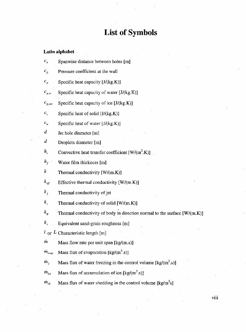
List of Symbols
Latin alphabet
Cp,w
Cp,ice
d
d
krp
Spanwise distance between holes [ml
Pressure coefficient at the wall
Specifie heat capacity [J/(kg.K)]
Specifie heat capacity of water [J/(kg.K)]
Specifie heat capacity of iee [J/(kg.K)]
Specifie heat of solid [J/(kg.K)]
Specifie heat of water [J/(kg.K)]
Jet hole diameter[m]
Droplets diameter [ml
Convective heat transfer coefficient [W/(m2.K)]
Water film thiekness [ml
Thermal conductivity [W/(m.K)]
Effective thermal conductivity [W/(m.K)]
Thermal conductivity of jet
Thermal conductivity of solid [W/(m.K)]
Thermal conductivity of body in direction normal to the surface [W/(m.K)]
ks Equivalent sand-grain roughness [ml
1 or L Characteristic length [ml
rh Mass flow rate per unit span [kg/(m.s)]
m evap Mass flux of evaporation [kg/(m2.s)]
mf Mass flux of water freezing in the control volume [kg/(m2.s)]
rhice Mass flux of accumulation of iee [kg/(m2.s)]
m sh Mass flux of water shedding in the control volume [kg/m2s]
viii
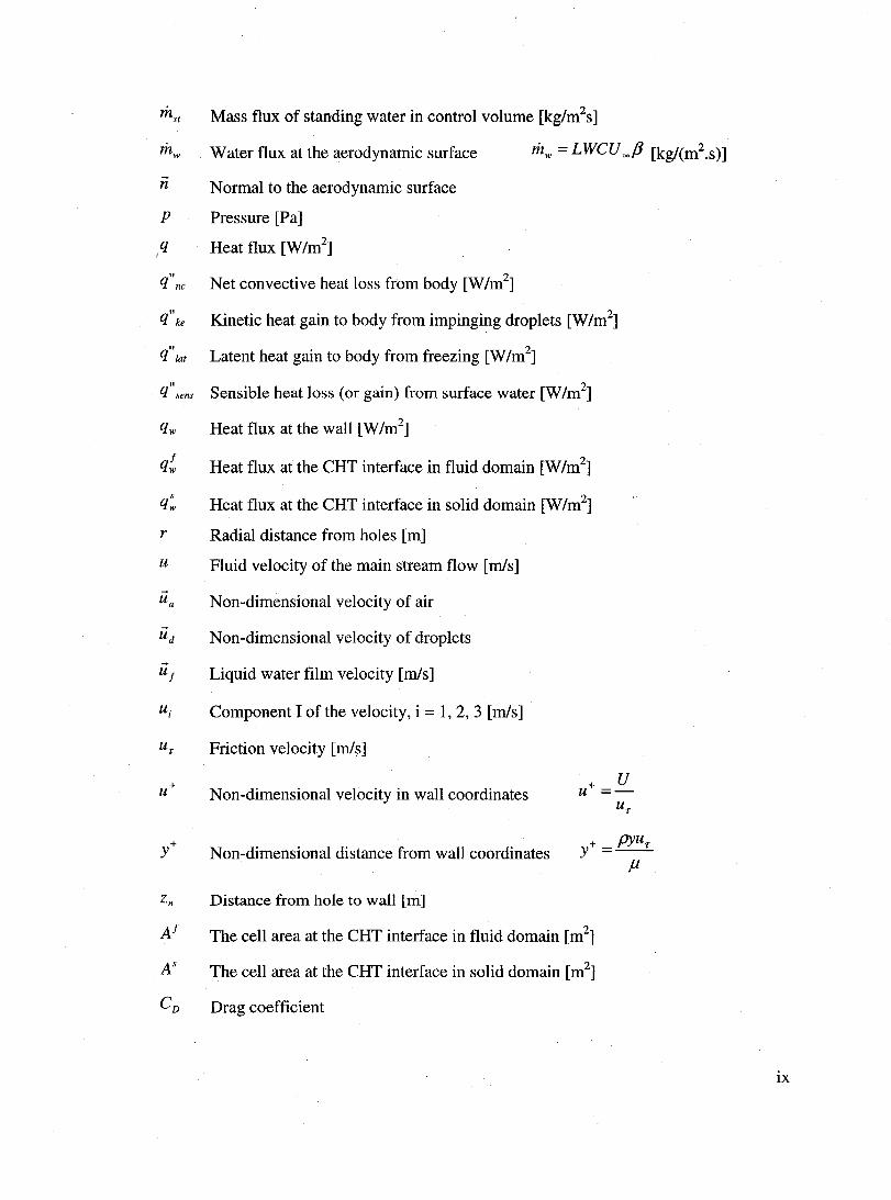
1
m.,·t Mass flux of standing water in control volume [kg/m2s]
n
p
q
q" ne
q" ke
q"lat
q" ... ens
r
u
A'
C D
Water flux at the aerodynamic surface
Normal to the aerodynamic surface
Pressure [Pa]
Heat flux [W/m2]
Net convective heat loss from body [W/m2]
Kinetic heat gain to body from impinging drop lets [W/m2]
Latent heat gain to body from freezing [W/m2]
Sensible heat loss (or gain) from surface water [W/m2]
Heat flux at the wall [W/m2]
Heat flux at the CHT interface in fluid domain [W/m2]
Heat flux at the CHT interface in solid domain [W/m2]
Radial distance from holes [ml
Fluid velocity of the main stream flow [mis]
Non-dimensional velocity of air
Non-dimensional velocity of droplets
Liquid water film velo city [mis]
Component 1 of the velocity, i = 1,2,3 [mis]
Friction velocity [mis]
Non-dimensional velocity in wall coordinates + U
u =-ur
Non-dimensional distance from wall coordinates + pyur y =--
Distance from hole to wall [ml
The cell area at the CHT interface in fluid domain [m2]
The cell area at the CHT interface in solid domain [m2]
Drag coefficient
fi
ix
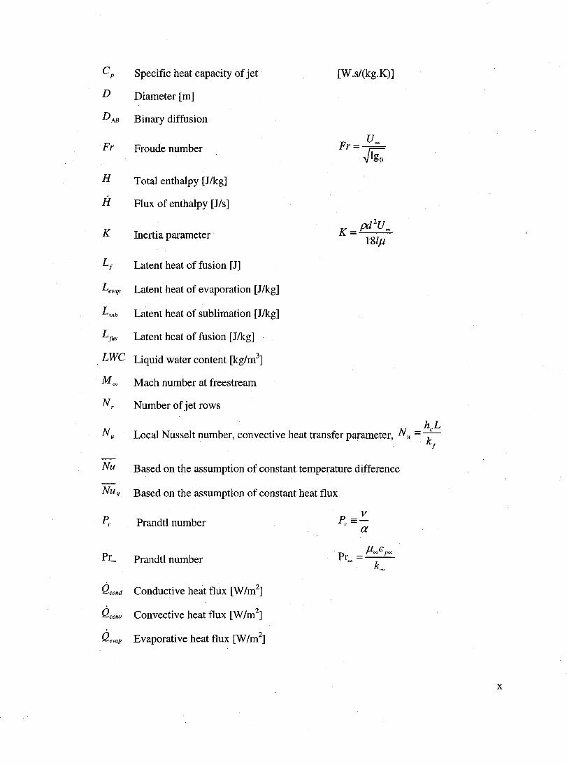
Cp
D
D AB
Fr
H
il
K
Lf
Levap
Lsub
Lfus
LWC
M=
Nr
Nu
NU q
Pr
Pr""
Qcond
Qconv
Qevap
Specifie heat capacity of jet
Diameter [m]
Binary diffusion
Froude number
Total enthalpy [J/kg]
Flux of enthalpy [J/s]
Inertia parameter
Latent heat of fusion [J]
Latent heat of evaporation [J/kg]
Latent heat of sublimation [J/kg]
Latent heat of fusion [J/kg]
Liquid water content [kg/m3]
Mach number at freestream
Number of jet rows
[W . s/(kg.K) ]
F U"" r = ~lgo
N hcL
Local Nusselt number, convective heat transfer parameter, u = T;
Based on the assumption of constant temperature difference
Based on the assumption of constant heat flux
V Prandtl number P=-r a
Prandtl number P Il,,,,c P""
r"" = k""
Conductive heat flux [W/m2]
Convective heat flux [W/m2]
Evaporative heat flux [W/m2]
x
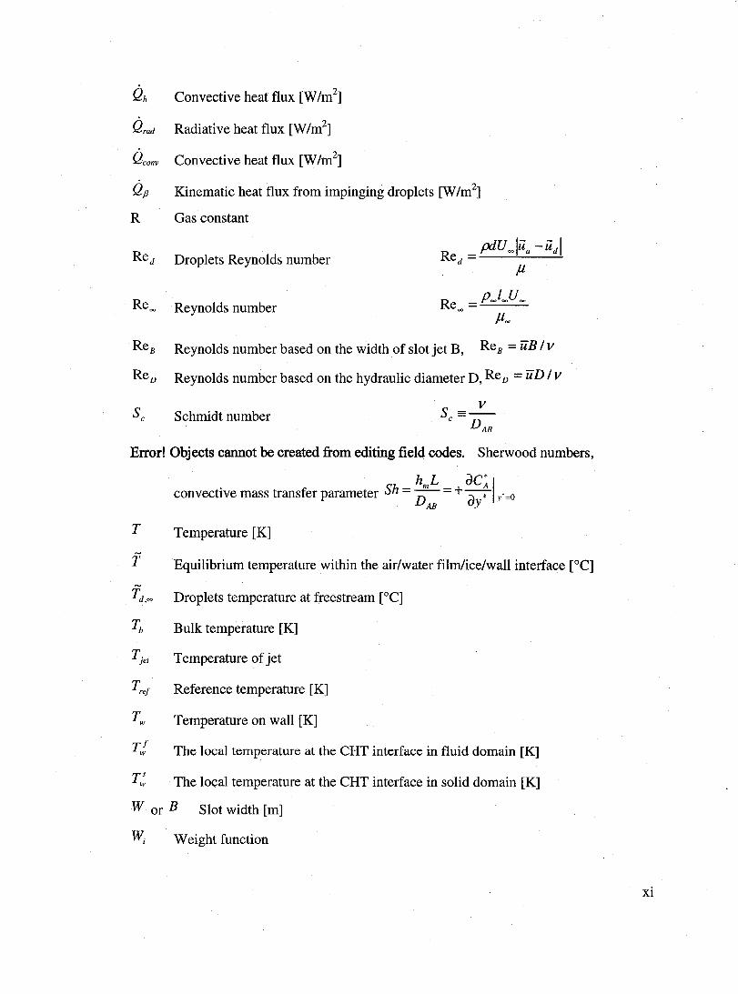
Qh Convective heat flux [W/m2]
Qrad Radiative heat flux [W/m2]
Qconv Convective heat flux [W 1m2]
Qp Kinematic heat flux from impinging droplets [W/m2]
R Gas constant
Re d Droplets Reynolds number pdU oolüa -üdl
Re d = ---'-----'-P
Re 00 Reynolds number Re = PooCU 00
00 Poo
ReB Reynolds number based on the width of slotjet B, ReB = ïiB Iv
ReD Reynolds number based on the hydraulic diameter D, ReD = ïiD Iv
Schmidt number S =~ c D
AB
Error! Objects cannot be created from editing field codes. Sherwood numbers,
h hmL ac~ 1 convective mass transfer parameter S = -D = +-;-;- y'=o
AB uy
T Temperature [K]
T Equilibrium temperature within the air/water film/ice/wall interface [OC]
Droplets temperature at freestream [oC]
Bulk temperature [K]
Temperature of jet
Reference temperature [K]
Temperature on wall [K]
The local temperature at the CHT interface in fluid domain [K]
T~ The local temperature at the CHT interface in solid domain [K]
W or B Slot width [ml
W; Weight function
xi

Greek alphabet
a Droplet volume fraction, ratio of the volume occupied by water over the total
volume of the fluid element
a Thermal diffusivity k f a=--
pep
P Local collection,effieiency P=-aud ·n
rp Direction normal to body surface [ml
r Ratio of specifie heat
a Boltzman constant [=5.670xlO-8 W/(m2.K4)]
ê Solid emissivity
f.1 Dynamic viscosity coefficient [kg/(s.m)]
f.1T Turbulence dynamic viscosity coefficient [kg/(s.m)]
V Kinematic viscosity [m2/s]
p Density [kg/m3]
Pa Density of air
Ps Density of solid
rii Shear stress tensor
rS ii Kronecker delta, i.e., rS ii
=1 if i=j and rS l; =0 if ilj
/).scurrent Surface distance spacing at CUITent location [ml
/).snext Surface distance spacing at next location [ml
Subscripts
conv Convection
cond Conduction
evap Evaporation
f Water film or fluid
xii

zee !ce accretion
imp Impinging water
in Entering a control volume
out Leaving a control volume
ref Reference value
s Solid
T Turbulence
r Boundary surface
00 Free stream value
xiii

List of Figures
Figure 1.1 Areas That May Require Ice Protection, Source: FAA, Technical Report ADS-
4, December 1963 ........................................................................................................ 2
Figure 1.2 Temperature Profile and Streamlines From the Piccolo Jet, Inside A 3D Wing
Slat [15] ....................................................................................................................... 5
Figure 2.1 The Empirical Method for Conjugate Heat Transfer Problem ........................ 10
Figure 2.2 CHT2D Anti-Icing Algorithm (From Reference [26]) ............ ; ....................... 20
Figure 2.3 Water Film Region (From Reference [32]) ..................................................... 21
Figure 2.4 The Construction of the Laval University Anti-Icing Experimental Assembly
(From Reference [33]) ............................................................................................... 23
Figure 2.5 The Flow Pattern of A Single Round or Slot Impinging Jet ............................ 25
Figure 4.1 The Hot-Air Anti-Icing Heat Transfer Processes ............................................ 44
Figure 4.2 The Overall Energy Balance in the Hot Anti-Icing System ............................ 47
Figure 4.3 The Methodology of CHT3D Anti-Icing Simulation ...................................... 49
Figure 4.4 The Flow Chart of CHT3D Algorithm ............................................................. 51
Figure 4.5 Dual Meshes on Structured Grid ..................................................................... 56
Figure 4.6 Construction of the Virtual Grid for A Square Surface: (A) Fluid and Solid
Grids at Fluid/Solid Interface; (B) Final Virtual Grid at Fluid/Solid Interface [47].58
Figure 4.7 Evaluation of A Surface Integral on the Virtual Grid [47]: the Red Triangle Is
A Solid Face and Blue Triangles Are Fluid Faces .................................................... 59
Figure 5.1 The Verification Test Case for CHT3D ............................................................ 62
Figure 5.2 Water Film Mass Flow on Upper Surface of the Flat Plate ............................. 63
Figure 5.3 Heat Flux Distribution on Upper Surface of the Flat Plate .............................. 63
Figure 5.4 Temperature Distribution on Both Surfaces of the Flat Plate .......................... 64
Figure 5.5 Water Film Mass Flow on Upper Surface of the Flat Plate ............................. 65
Figure 5.6 Heat Flux Distribution on Upper Surface of the Flat Plate .............................. 65
Figure 5.7 Temperature Distribution on Both Surfaces of the Flat Plate .......................... 66
Figure 5.8 Water Film Mass Flow on Upper Surface of the Flat Plate ............................. 67
Figure 5.9 Heat Flux Distribution on Upper Surface of the Flat Plate .............................. 67
Figure 5.10 Temperature Distribution on Both Surfaces of the Flat Plate ........................ 67
xiv

Figure 5.11 Convective Heat Flux Distribution on the Upper Surface of the Flat Plate .. 68
Figure 5.12 Temperature Distribution on Both Surfaces of the Flat Plate ........................ 68
Figure 6.1 Fully Developed Laminar Slot Jet with 1mpingement on a Flat Plate ............. 70
Figure 6.2 Mesh with 11800 Nodes for Spalart-Allmaras Turbulence Mode!.. ................ 73
Figure 6.3 y+ of the First Layer Nodes Away From Impinging Wall .............................. 73
Figure 6.4 Mach Number Distribution Solved with Spalart-Allmaras Model .................. 74 \
Figure 6.5 Mesh with 5880 Nodes for k-E Turbulence Mode!.. ........................................ 75
Figure 6.6 Mach Number Distribution Solved with k-E High Reynolds Model ............... 75
Figure 6.7 Comparison of Local Nusselt Number between k~E Model, Spalart-Allmaras
Model, and Experimental Result ............................................................................... 76
Figure 6.8 The Geometry of the Simplified Anti-Icing Test Case .......................... ; ......... 77
Figure 6.9 The Wind Tunnel Section ................................................................................ 77
Figure 6.10 The Aluminum Flat Plate Section .................................................................. 78
Figure 6.11 The 1mpinging Jet Section ............................................................................. 78
Figure 6.12 The Partial Mesh of the Wind Tunnel Airflow .............................................. 79
Figure 6.13 !nlet Velocity Profile of Wind Tunnel Air Flow ........................................... 80
Figure 6.14 The Mach Number Distribution of the Wind Tunnel Airflow ....................... 80
Figure 6.15 Comparison of the Pressure Coefficient on the Wind Tunnel Floor with
Experimental Result .................................................................................................. 81
Figure 6.16 The Mesh of the 1mpinging Jet flow .............................................................. 82
Figure 6.17 The Mach Number Contour Lines of Jet Flow .............................................. 83
Figure 6.18 Comparison of Heat Transfer Coefficient Distribution on Impinging Surface
........................................................... ~ ........................................................................ 84
Figure 6.19 The Mesh of the Aluminum Flat Plate ........................................................... 85
Figure 6.20 CHT3D Convergence History of the Temperature on the Flat Plate Upper
Surface ......................................................... ; ....................................................... ; ..... 86
Figure 6.21 Heat Transfer Coefficients on Both Surfaces of Aluminum Flat Plate ......... 87
Figure 6.22 Convective Heat Fluxes on Both Surfaces of Aluminum Flat Plate ............... 87
Figure 6.23 Temperature Distribution in the Aluminum Plate (The Thickness of the Plate
1s Scaled for Better View) ......................................................................................... 88
xv
Figure 6.24 Temperature Distributions on Both the Upper and Lower Surfaces of
Aluminum Flat Plate .................................................................................................. 88
Figure 6.25 Comparison of Heat Fluxes on Upper Surface of the Aluminum Flat Plate
between CHT3D Calculation and Experimental Result with Error Bar ................... 89
xvi
List of Tables
Table 6.1 Boundary Conditions for Slot Impinging Jet Test Case .................................... 72
Table 6.2 Boundary Conditions for the Wind Tunnel Airflow ......................................... 79
Table 6.3 Boundary Conditions for the Impinging JetFlow ............................................. 82
xvii

CHAPTER 1: Introduction
1.1 In-flight lcing Phenomena
In-flight icing is a major aviation hazard that seriously threatens flight safety and has been
the cause of several aircraft accidents, such as the accidents of American Eagle ATR-72
in 1994 and Embraer EMB-120 in 1997 [1]. A recent survey of commercial pilots
indicates that the frequency of icing encounters is quite high, with de-icing devices
having to be activated on up to 80% of turboprop flights [2]. Therefore, the guaranteed
protection of aircraft surfaces and critical engine components against ice or iceeffects
remains a major concern to aircraft and engine manufacturers and to certification
regulators.
When an aircraft flies through clouds under icy conditions, supercooled water droplets at
temperatures below the freezing point may impact on aircraft surfaces and result in ice
accretion. The ice accretion on critical surfaces of an aircraft such as wings, propellers
and stabilizers can have a significant impact on operation and controllability of an aircraft.
It may increase the total weight of the aircraft, shift its center of gravit y, freeze the
movable components such as flaps and slats and deteriorate the aerodynamic properties of
airflow causing a substantial decrease of lift, increase in drag, and reduction of stall
margin. The accreted ice on the nacelle or the wing in front of an engine may be ingested
into the engine inlet as foreign object damage (FOD) , therefore causing power
fluctuations, thrust loss, roll back, flame out and loss of transient capability [3].
There are three types of icing formations: rime ice, glaze ice and mixed ice [3]. Rime ice
usually occurs at low temper~tures from -40 to -10°C, low airspeed and low Liquid
Water Content (LWC). In this situation, all the super-cooled water droplets that impact on
a surface will freeze immediately. Rime ice still has a reasonable aerodynamic shape but
with higher surface roughness, that greatly increases the aerodynamic drag.
1
Glaze ice appears at higher temperatures from -3 oC up to the freezing point of water,
high airspeed and high L Wc. The ice is formed from runback water and ha's the shape of
horns or lobster tails that have less surface roughness but create a big change in original
airfoil shape and cause the separation of airflow. Mixed ice is the combination of rime
ice and glaze ice.
1.2 In-flight lcing Protection and Aircraft AntilDe-lcing Systems
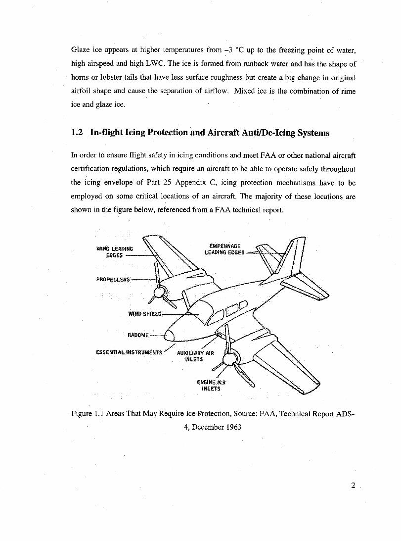
In order to ensure flight safety in icing conditions and meet F AA or other national aircraft
certification regulations, which require an aircraft to be able to operate safely throughout
the icing envelope of Part 25 Appendix C, icing protection mechanisms have to be
employed on sorne critical locations of an aircraft. The majority of these locations are
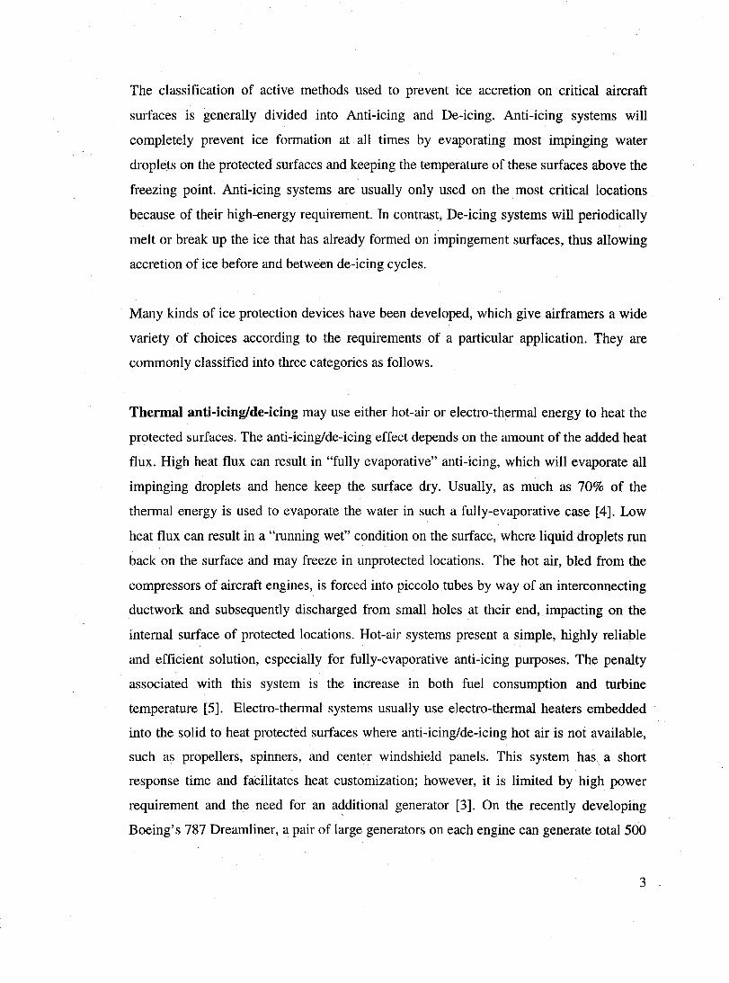
shown in the figure below, referenced from a F AA technical report.
EMPENNAGE lEADING EOGES -~""""'''''''''''''''f
wmc l.EADING EOGES ---->Ir'\
PR()PfLLERS ---hl
ESSENTIAL INSTRUMENTS / AUXlllARV AIR INtElS
Figure 1.1 Areas That May Require Ice Protection, Source: F AA, Technical Report ADS-
4, December 1963
2
The classification of active methods used to prevent ice accretion on critical aircraft
surfaces is generally divided into Anti-icing and De-icing. Anti-icing systems will
completely prevent ice formation at aIl times by evaporating most impinging water
droplets on the protected surfaces and keeping the temperature of these surfaces above the
freezing point. Anti-icing systems are usually only used on the most critical locations
because of their high-energy requirement. In contrast, De-icing systems will periodically
melt or break up the ice that has already formed on impingement surfaces, thus allowing
accretion of ice before and between de-icing cycles.
Many kinds of ice protection devices have been developed, which give airframers a wide
variety of choices according to the requirements of a particular application. They are
commonly classified into three categories as follows.
Thermal anti-icing/de-icing may use either hot-air or electro-thermal energy to heat the
protected surfaces. The anti-icing/de-icing effect depends on the amount of the added heat
flux. High heat flux can result in "fully evaporative" anti-icing, which will evaporate aIl
impinging droplets and hence keep the surface dry. UsuaIly, as much as 70% of the
thermal energy is used to evaporate the water in such a fully-evaporative case [4]. Low
heat flux can result in a "running wet" condition on the surface, where liquid droplets run
back on the surface and may freeze in unprotected locations. The hot air, bled from the
compressors of aircraft engines, is forced into piccolo tubes by way of an interconnecting
ductwork and subsequently discharged from small holes at their end, impacting on the
internaI surface of protected locations. Hot-air systems present a simple, highly reliable
and efficient solution, especially for fully-evaporative anti-icing purposes. The penalty
associated with this system is the increase in both fuel consumption and turbine
temperature [5]. Electro-thermal systems usually use electro-thermal heaters embedded
into the solid to heat protected surfaces where anti-icing/de-icing hot air is not available,
such as propellers, spinners, and center windshield panels. This system has a short
response time and fadlitates heat customization; however, it is limited by high power
requirement and the need for an additional generator [3]. On the recently developing
Boeing's 787 Dreamliner, a pair of large generators on each engine can generate total 500
3 .
kilovolt-amps (kva) power per engine, which is more than four times the amount of
power extracted from engines on other aircraft. This innovative design makes it possible
to run aIl aircraft systems by electricity and to essentially eliminate the bleed air from
engines. On this so-called all-electric airplane, electric heat will be used for the anti-icing
of the wing, which needs a large electrical load of approximate 1 OOkw. The only
remaining bleed air is used for the engine inlet anti-icing [6].
Boots, or mechanical de-icing is designed to break and shed the ice from protected
surface into the air stream by suddenly deforming the iced surface. A lot of surface
deformation systems have been developed for mechanical de-icing, such as Pneumatic
Boot Systems, Pneumatic-impulse De-icing Systems, Electro-mechanical Expulsive De
icing Systems (EMEDS), Electro-impulse De-icing Systems (EIDI) , Eddy CUITent De
icing Systems (ECDS), Electro-expulsive De-icing System (EEDS) and Shape Memory
Alloys.
The boot is not an anti-icing device but a de-icer. Rence, a minimum initial ice is needed
for boot to be effective. Moreover, the mechanical de-icing systems cannot operate
continuously and they are intermittent by nature with blackout periods as the cycle can
only do wings, empennage, etc. in sequence. As a result, inter-cycle and intra-cycle ice
may form. In addition, residue ice may remain after each de-icing cycling due to the less
effective of these systems for thin ice.
Fluid protection system prevent the accretion of ice by using freezing point depressant
fluids (FPD), usually deposited by spray bar of windshield, slinger ring and inertia of
propeller, and porous wing surfaces to reduce the freezing point. It is limited by fluid
supply, weight, and expense.
Of aIl anti/de-icing mechanisms discussed above, the hot bleed air systems are the most
reliable and efficient ones, and are therefore widely used on critical ice protection regions
of most commercial aircraft, such as leading edge wing panels and high lift devices,
empennage surfaces, engine inlet and air scoops, radomes, and sorne types of instruments. .
4

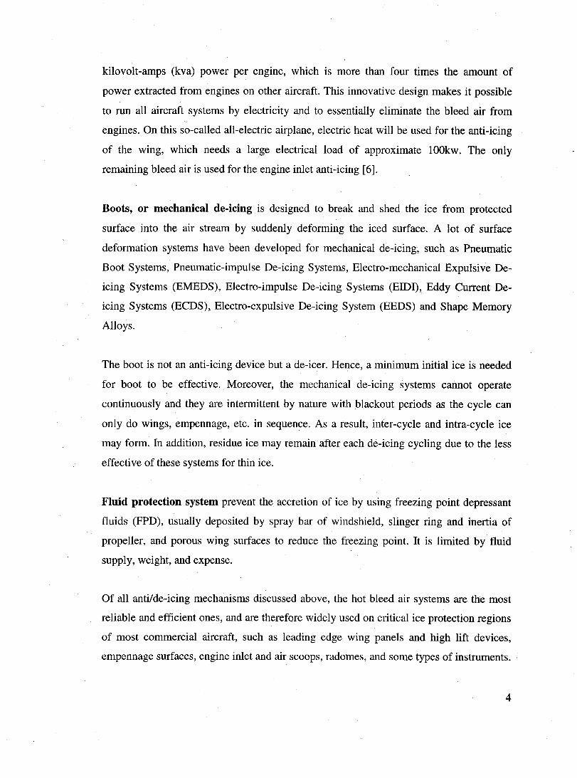
The following figure shows the numerical simulation of a typical 3D hot-air anti-icing
device detailing the complex 3D nature of the jet flow around a piccolo tube inside a wing
slat, which was performed by Croce, Habashi et al. [15].
Figure 1.2 Temperature Profile and Streamlines From the Piccolo Jet, Inside A 3D Wing
Slat [15]
1.3 CFD Tools for In-Flight Icing and AntilDe-Icing Analysis
Traditionally, the icing, anti/de-icing analysis and icing certifications were performed by
a combination of simulation methods that comprise CFD, icing tunnels and by tanker
testing, and by natural flight testing. The combination orthe above methods often cannot
simulate and test the full range of the icing env el ope required by FAR Part 25 Appendix
C, because each exhibits sorne deficiencies [7].
The icing tunnel experimental testing is usually done at low Reynolds number (Re) and
cannot simply extrapolate the result to high R~ for larger aircraft, as the scaling process is
highly nonlinear. The results from different icing tunnels often present sorne
disagreement and the experimental result cannot be repeated in sorne tunnels. The errors
may also be due to the partial geometries tested, relatively primitive ice shape
measurement techniques, tunnel wall effects and scaling techniques for controlling icing
parameters, still a maturing area of research.
5
Flight-testing behind a tanker features the following deviations from natural in-flight
icing conditions:
• the generation of supercooled droplets is not possible due to the impurity of tanker
water
• the dyed water may cause more runback effect than supercooled water
• the tanker moves when the droplets are released
• the droplets AoA is not exactly the same as the aircraft AoA because of the width
and breadth of the spray
• more uncertainties may also be caused by the sub-saturated condition, droplets
evaporation, coagulation, break-up and spectra limitations
• No real measurements can be made during flight, only qualitative observations
Natural flight-testing has seasonallimitations and is risky in sorne extreme situations. It is
not completely gene~al and not suitable to qualify ice shapes or performance effects.
Moreover, ice accretions on sorne locations are difficult to be observed, such as on the
wing tips, bottom of wings, or on top of high-wings.
In recent years, with the dramatically increased computational power and decreased co st
to solve the Navier-Stokes equations of complex 3-D fluid flows, accurately capturing the
physics of the flow has become realistic. Computational Fluid Dynamics (CFD) has been
playing an important role in in-flight icing analysis, anti-/de-icing system design and
airworthiness certification, such as the design of icing tunnel models, determining worst
case scenarios for icing encounters, estimating the ice shapes and aerodynamics penalties
for delayed turn-on and failure cases and for unprotected surfaces, estimating temperature
and heat flux of anti-icing system, completingstudy of design parameters for preliminary
anti-/de-icing system design and optimization of anti-/de-icing system. Comparing with
traditional methods, CFD analysis has shown advantages such as reducing and focusing
experiments and flight tests, shortening the development period, flexibility for
optimization design and parameter study, simulating a wider range of icing condition,
avoiding experimental assumptions and measurement errors, capability to analysis the
whole anti-/de-icing system with much more detailed data than measurement at
6
instrumented areas [7]. On the other hand, CFD analysis also has its disadvantages, which
may arise from neglecting sorne physical phenomena in the mathematical equations,
inaccuracy of numerical discretization, incomplete convergence and instability of
numerical calculations, etc. Therefore, CFD analysis still needs to combine with other
methods for engineering applications.
More and more countries and aerospace companies have been engaging in their own icing
and anti-/de-icing research and CFD tools development such as LEWICE from Glenn
Icing Research Center of NASA in V.S. [8], ONERA-ICE from ONERA in France,
CANICE from Bombardier Aerospace in Canada [9], FENSAP-ICE from Newmerical
Technologies International Canada [10]. LEWICE is a 2D ice accretion numerical model
originally designed for solving the flow field, droplets trajectory and impingement, and
ice accretion. It has also expanded for hot-air or electro-thermal anti-icing simulations.
CANICE is also a 2D ice accretion model based on the similar algorithm as LEWICE.
FENSAP-ICE is a fully 3D CFD package including 3D Navier-Stokes airflow model, 3D
Eulerian droplet impingement model, 3D ice accretion thermodynamic model, 3D mesh
optimization tool and 3D conjugate heat transfer model.
1.4 Objective of Current Work
The FENSAP-ICE package developed by CFD Lab of McGill University and
Newmerical Technologies International (NTI) is a state-of-the-art 3D modular simulation
tool to analyze the aerodynamics, droplet impingement, ice accretion, and thermal
properties of any anti-icing system. The objective of this thesis is to develop a three
dimensional conjugate heat transfer (CHT) module labeled CHT3D, based on FENSAP
ICE's capabilities, to simulate the complicated thermal processes of aircraft hot-air anti
icing systems. This procedure is based on a continuous exchange of boundary conditions
at fluid/solid and fluid/water interfaces. It couples together a Navier-Stokes flow solver
(FENSAP), an Eulerian droplet impingement module (DROP3D), a 3D ice accretion
module (ICE3D) and a solid conduction module (C3D). Such a general CHT3D
procedure can also be applied to other CHT problems such as mist-cooled heat
exchangers, turbine blade cooling, automotive and aircraft brake cooling, etc.
7

A literature review of CHT methodologies and anti-icing simulations is presented in
chapter 2. The mathematical governing equations and numerical methods used for the
entire anti-icing simulation are discussed in chapter 3. In chapter 4, a loose-coupling CHT
algorithm has been developed and implemented for anti-icing simulations and will be
elaborated. In chapter 5, a test case shows the capability of CHT3D in simulating a span
of anti-icing and de-icing cases: fully evaporative, running wet, or iced; A jet
impingement test case is implemented for validating different turbulence models in the
airflow sol ver for predicting the heat transfer properties of the impinging slot jet; The
CHT3D procedure is finally validated against a 2D dry air experimental test case from
Laval University, because of the dearth of appropriate open literature 3D test data.
8
CHAPTER 2: Literature Review
2.1 Methodology of Conjugate Heat Transfer Calculation
In a typical anti-icing system of an aircraft wing, the hot air is bled from engme
compressors, ducted into a piccolo tube from the pneumatic manifold and impinged on
the internaI front surface of the wing to prevent ice accretion on the external surface.
Modern turbofan engines are designed with higher and higher bypass ratios in order to
improve fuel economy and noise control, causing a decrease of the core engine size, thus
limiting the available bleeding air. Therefore, maximizing the anti-icing efficiency in
order to minimize bleed air becomes increasingly crucial in anti-icing system design to
reduce the performance penalties of turbofan engines. For this purpose, CFD numerical
too~s are continuously being developed to assist in designing efficient anti-icing systems
and in certification [7]. Similarly, in a jet engine, cooling air is deviated to high thermal
load regions to reduce turbine blade temperature and prevent material failure. Both
applications rely on the same heat transfer process, which inc1udes heat conduction
through a solid and heat convection caused by both internaI and external airflows.
Many numerical models have been developed for solving these types of heat transfer
problems, and are generally divided into empirical and conjugate methods. Empirical
methods do not take into account the interaction between the flow medium and the solid,
using empirical correlations to predict the convective heat loads due to airflows on solid
surfaces and are widely used in industry. Conjugate methods would be based on the
iterative exchange of boundary conditions at each fluid-solid interface until thermal
equilibrium is eventually achieved at each interface. This is the approach retained in the
present thesis.
2.1.1 Empirical Method for Heat Transfer Problems
In this approach, the local heat transfer coefficients and fluid reference temperatures (or
bulk temperatures) on both internaI and external solid walls are evaluated from empiricai
formulae, prior to their use as boundary conditions of the heat conduction calculation to
9

determine the temperature distributions in a solid body. The empirical method is shown
schematically in Figure 2.1 below.
/ " Evaluation of
he and Tref at
external surface \.
l Heat conduction Temperatures
in the solid in the solid body
r / " Evaluation of
he and Tref at
internaI surface /
Figure 2.1 The Empirical Method for Conjugate Heat Transfer Problem
Chmielniak et al.[ll] solved a turbine blade cooling problem with both empirical and
conjugate methods. In their calculations based on the empirical method, the fluid velocity
of the mainstream flow and the fluid temperature at the blade wall are obtained by solving
the fluid flow problem assuming adiabatic boundary conditions at the blade wall. Then
the local heat transfer coefficients at the blade wall can be calculated from empirical
formulae, which are based on the previously calculated fluid velocity and temperature at
the blade wall. It can be simply expressed as the following relationship:
(2.1)
Solving the problem with the empirical method is simpler and faster than using the
conjugate method because the local heat transfer coefficients are based on empirical
formulae and the airflow solution does not need to be updated. But the accuracy of the
10
results from empirical methods is very limited. One reason is the inaccuracy of the
empirical formulae themselves to predict the local heat transfer coefficients. Another
reason is that the fluid velocities and temperatures obtained from airflow computation are
not updated inuncoupled methods and are only based on the adiabatic wall boundary
condition, which is not a physically representative boundary condition. Thus, it will cause
another source of error in the ca1culations of empirical forrnulae, which are based on
above velocity and temperature. As well, the empirical formulae are application- and
geometry-dependent and accurate correlations are difficult to obtain for complicated and
three-dimensional geometries, thus the applicability of empirical methods to solve heat
transfer problems is greatly restricted.
2.1.2 Conjugate Method for Heat Transfer Problems
The Conjugate Heat Transfer (CHT) method iteratively solves the thermal interactions
between fluid and solid domains. In this method, multi-domains are used to separate
individual fluid and solid fields, and each domain has its own mesh. The coupled method
can directly ca1culate the heat transfer loads at fluid-solid interfaces instead of using
empirical correlations and its result is more accurate than empirical methods, but it needs
more computational power and longer times. The conjugate method can be represented by
two different approaches: the tight-coupling method and the loose-coupling method. The
loose-coupling method is the one used in the present anti-icing simulation. Both coupling
methods are based on the same conception, which ensures temperature and heat flux
equality conditions at each CHT interface a~ follow:
T!· = T; (2.2)
and·
(2.3)
2.1.2.1 Tight-Coupling Approach
In this approach, the heat conduction code is embedded into a CFD code, facilitating the
solution of fluid flow and heat conduction by a single code. It is a very robust and stable
coupling method because no further iteration process is required.
11
Marini [12] embedded the CHT capability into FENSAP, a finite element based Navier
Stokes CFD sol ver. In his work, the CHT problem is treated as a multi-domain problem
and each domain has individual mesh. The meshes of aIl domains are later combined
together inside FENSAP so that the solid energy equation and the fluid energy equations
can be solved simultaneously in a full y implicit manner. A special treatment, instead of
the nodal connectivity, is used to guarantee the equality conditions of temperatures and
heat fluxes at the CHT interface. The nodes in the fluid grid at the CHT interface are
termed 'dead' nodes and any other nodes in both fluid and solid grids are termed 'live'
nodes. Similarly, the elements in the fluid grid at the CHT interface are termed 'dead'
elements and any other elements in both fluid and solid grids are termed 'live' elements.
The energy equations of both liquid and solid domains are discretized and simultaneously
solved by the finite element method. The local element matrixes of aIl the live elements
are assembled into global matrix using the standard finite element method according to
the node connectivity of the meshes, so that, aIl live nodes have a direct representation in
the global matrix and are directly solved by the matrix sol ver. In dead elements, which
are the elements on the CHT interface in the fluid domain, the dead fluid nodes have an
indirect representation in the global matrix and their contributions are communicated
through the surrounding live solid nodes at the CHT interface. Therefore, at CHT
interfaces, temperatures of the nodes belonging to solid domain are directly solved for
and updated through the iterative solver. Temperatures in the fluid domain at the same
interface are not directly solved by the matrix sol ver and are interpolated from the values
of live solid nodes. Hence, the temperature equality in equation (2.2) is automatically
guaranteed. The heat fluxes are forced to be identical at the CHT interface due to the
implicit treatment in the weak-Galerkin finite element formulation. When the energy
equations of fluid and solid domain are solved, it is assumed that surface integral terms in
the weak-Galerkin residues of the fluid energy equation and the solid energy equation
cancel out each other at the CHT interface. That is:
12
After canceling out the same terrns on both sides of the equation, one can get the
simplified form:
(2.5)
Hence, the heat flux equality at the CHT interface is guaranteed by this assumption.
2.1.2.2 Loose-Coupling Approach
This approach couples CFD code, structure conduction code, and other numerical thermal
codes, such as ice accretion and fogging, externally only via a continuous and iterative
exchange of boundary conditions. Field equations in each computational domain are
solved individually to provide boundary conditions for the start of ca1culation of adjacent
computational domains. The loose-coupling approach works as a pure interfacial
algorithm and is completely independent from the details of existing solvers of each
computation al domain. Theoretically, it can couple any number of domains to simulate
very complicated conjugate heat transfer problems such as hot-air anti-icing. It has great
flexibility to use any available CFD code using heterogenous numerical discretization
schemes. Thus, the loose-coupling method is thought to be the most efficient and versatile
for complex conjugate heat transfer simulations. Numerical instability of loose-coupling
approaches can be eliminated by properly choosing boundary conditions in each domain
and using under-relaxation schemes during boundary condition exchanges. Giles [13] has
used a simple one-dimensional finite difference mode to study the numerical stability of
loose-coupling approach in fluid/structure thermal analysis and has shown that imposing
temperature boundary conditions (Dirichlet boundary conditions) for the fluid ca1culation
and heat flux boundary conditions (Neumann boundary conditions) for the structural
ca1culation will achieve numerical stability, but that in contrast imposing heat flux
boundary conditions (Neumann boundary conditions) for the fluid ca1culation and
temperature boundary conditions (Dirichlet boundary conditions) for the structural
ca1culation willlead to numerical instability, unless extremely small time steps are used.
Croce et al. have developed a loose-coupling approach [14] for CHT ca1culations and
have successfully implemented thermal analysis for an anti-ici.ng device [15], a mist-flow
13
heat exchanger [16] and turbomachinery compressible flow applications [17]. This
approach corresponds to the Shur Complement algorithm for domain decomposition of
partial differential equations described by Funaro et al. [18] and can be summarized as
follows:
1. Solve Navier-Stokes equations in fluid domain with Dirichlet boundary conditions
(T k) at the CHT interface.
2. Evaluate the heat flux distribution at the CHT interface from the fluid solution.
3. Solve the heat conduction equation in solid domain with the Neumann boundary
condition from step 2 at the CHT interface.
4. Evaluate the temperature at the CHT interface (Tr ) from the conduction solution.
5. Use a relaxation parameter to update the temperature distribution at the CHT
interface as follows:
(2.6)
6. Use the new temperature distribution as Dirichlet boundary condition to solve the
Navier-Stokes equations in fluid domain.
7. Repeat steps 2 to 6 until convergence is achieved.
Imlay et al. [19] have tried two different loose-coupling procedures to couple the Navier
Stokes and heat conduction modules at each time step. The first procedure is exactly the
same as Croce's approach, but without under-relaxation in Imlay's application. This
approach led to wild oscillations and instabilities of wall temperatures. In his second
procedure, the instability of the coupling was damped by imposing a Robin boundary
condition to the structure conduction module instead of the Neumann boundary condition.
The reference temperatures (T,ef) are the stagnation temperatures of the fluid at first
nodes away from the wall. Then, local heat transfer coefficients can be evaluated from
equation (2.7).
qw = h(Tw - Tref )
This coupling procedure is described as follow:
(2.7)
1. Solve Navier-Stoke equations to update the heat flux distribution at the fluid-solid
interface with a given temperature distribution at the interface.
14
2. Calculate the reference temperature distribution (TreJ ).
3. Calculate the heat transfer coefficient distribution (h) using equation (2.7).
4. Pass the heat transfer coefficient distribution and the reference temperature
distribution at the interface from the fluid grid to the structure grid.
5. Solve the heat conduction code to update the temperature distribution (Tw ) at the
fluid-solid interface.
6. Pass the temperature distribution (Tw ) at the interface from the structure grid to
the fluid grid.
7. Repeat step 1 to 6 until a convergence is achieved.
In the coupling procedure above, the reference temperature distribution is determined first
and then is used to calculate the heat transfercoefficient distribution. However, Montenay
et al. [20] use an opposite way to obtain the Robin boundary condition. In their procedure,
a constant heat transfer coefficient a is chosen first at the CHT interface and is fixed in
aIl coupling steps. The reference temperature distribution at the CHT interface will be
updated in each CHT iteration based on the fixed heat transfer coefficient distribution and
the solution of puid domain as shown in equation (2.8).
, J,n
T n =Tf,n_~ ref w a
(2.8)
In this procedure, the Robin boundary condition is considered as a kind of relaxation to
the solid conduction calculation. The heat flux distribution at the CHT interface can be
post-evaluated from the temperature distribution of the conduction solution as follows:
q .l',n+l = a(T.I',n+l _ T n.) w w rq (2.9)
Combining the above two equations, one can get:
(2.10)
which can also be expressed as:
( .l',n+l f,n)
Ts,n+l =Tf,n + qw -qw w w a (2.11)
15

This equation indicates that the big heat transfer coefficient (a ) will relax the ,
temperature variations from last iteration. Therefore, the higher heat transfer coefficient
( a ) will increase the stability of the CHT coupling and reduce convergence speed.
Kassab et al. used a loose-coupling approach to couple the NASA-Glenn turbomachinery
FVM Navier-Stokes solver and a BEM steady state heat conduction code for solving the
CHT problem of film-cooled turbine blades. In this coupling approach, a Neumann
boundary condition is imposed for solid conduction calculation and a Dirichlet boundary
condition is imposed for Navier-Stokes calculation, which is opposite to the suggestion of
Giles' study [13]. Hence, very small time marching interval was used for the coupling
between the fluid and solid solvers in their simulations in order to stabilize the CHT
calculation. Their procedure can be described as follows:
1. Solve the fluid domain by the FVM Navier-Stokes sol ver with an initial adiabatic
boundary condition at the CHT interface to get a temperature distribution at the
CHT interface.
2. Impose the temperature distribution at the CHT interface to the BEM conduction
solver to evaluate the heat flux distribution at the CHT interface.
3. Relax the heat flux distribution before transferring them to the FVM solver.
R REM (1 fJ) REM q = J-iqold + - qnew (2.12)
where, fJ is a relaxation parameter and a greater value of fJ corresponds to a
higher relaxation. 0.2 is used in their application.
4. Impose the heat flux distribution to the FVM Navier-Stokes sol ver to calculate the
temperature distribution at the CHT interface.
5. Repeat steps 2 to 4 until the convergence of temperature and heat flux
distributions are obtained.
2.2 Overview of Numerical Simulations for Aireraft Hot-Air Anti-lcing
Systems
From the above discussions, the implicit coupling approach is a robust and stable method
for the application of unsteady problems or when time accuracy is critical. However, it is·
16
difficult to implement for complicated applications with more than two domains, such as
anti-icing simulation, where droplet impingement and water filmlice accretion
calculations need to be included into the coupling as weIl. To simultaneously solve so
many domains including a large set of equations is daunting. Furthermore, the mismatch
in the structure of the coefficient matrices is a great difficulty if different types of sol vers ,
such as FEM, FVM, or BEM, are used for different computational domains. The 100 se
coupling approach is the most practical and simplest method for complicated CHT
problems because it only increases the complexity of the coupling itself, instead of
changing any detail of the numerical solvers. It is also very flexible to replace solvers for
each domain with minimum modifications of the coupling code. Therefore, the loose
coupling approach is strongly suggested for aircraft hot-air anti-icing simulations.
However, only limited literature is available for fully CFD-based simulations of entire
hot-air anti-icing processes.
2.2.1 Hot-Air Anti-Icing Simulation in LEWICE
LEWICE is an ice accretion prediction code developed by NASA Glenn Research Center.
It also has the capability to analyze the performance of electro-thermal deicers or hot-air
anti-icing systems based on the numerical model of AI-Khalil [22]. It consists of four
modules: the flow field calculation, the particle trajectory and impingement calculation,
the thermodynamic and ice growth calculation, and the modification of the geometry due
to the ice accretion [8]. The airflow solver in LEWICE is based on a Douglas 2D
potential flow panel method program developed by Hess and Smith [23] for an inviscid
velocity field, and an integral boundary layer calculation for viscous effects in the
boundary layer. Recently, a 3D version of the panel method has been developed to enable
LEWICE to calculate the airflow in 3D [8]. The droplet impingement calculation in
LEWICE is based on particle tracking techniques, in which a particle is launched from
the free stream and is dragged by the airflow until hitting or not the body. These
techniques are very efficient on 2D and simple geometries, but become computationally
expensive in 3D and encounter major difficulties on complex geometries, especially when
the appropriate launch area may not be known a priori. The thermodynamic analysis of
17

the icing surface is based on the Messinger's thermodynamic model [24], which includes
the equations of mass and energy balances in a control volume.
The mass balance equation evaluates the amount of the water mass entering and leaving
the control volume and can be expressed as [8]:
. . . . . /1snext • • m imp + min = m evap + m f + mout + m,,'h + mst
/1s eurrent
(2.13)
The energy balance equation, obeying the first law of thermodynamics, evaluates the
amount of the heat entering and leaving from the control volume and can be expressed as
[8]:
( k dT J -" + Il + Il + " + " - a - q ne q evap q ke q lat -q sens ~ cp '1'=0
(2.14)
In LEWICE hot-air anti-icing simulations, a ID heat conduction in the normal direction
through the surface is assumed. This assumption ~tates that the heat conduction through a
solid surface is primarily ID if anti-icing processes have a 3D internaI hot airflow, and a
primarily 2D external airflow and water collection. In their anti-icing model, the heat
transfer coefficient on the solid internaI surface was determined based on empirical
correlations rather than directly solving the 3D internaI jet flow from the CFD solver. The
empirical correlations were designed to evaluate the local and average Nusselt numbers
for arrays of circular holes impinging normally on a flat plate, which has a vaguely
similar geometry to the piccolo tube of aircraft anti-icing system. The local and average
Nusselt numbers can be evaluated and are primarily a function of the jet Reynolds
number, the jet spacing, and the distance to the wall. The Reynolds number for circular
cross-section holes can be calculated by using the mass flow rate per unit span as:
Re= 4liz .s.. 1lNr f.1 d
(2.15)
18
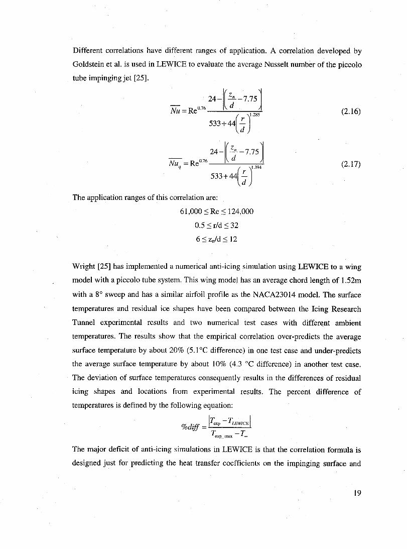
Different correlations have different ranges of application. A correlation developed by
Goldstein et al. is used in LEWICE to evaluate the average Nusselt number of the piccolo
tube impinging jet [25].
_ 24-(~-7.75 J Nu ~ReO.76 533+44(~ J285
_ 24- (~-7.75 ~ 0.76 d ~
NUq = Re 1.394
533+44(~ ) The application ranges of this correlation are:
61,000:::; Re:::; 124,000
0.5:::; r/d:::; 32
6:::; zuld:::; 12
(2.16)
(2.17)
Wright [25] has implemented a numerical anti-icing simulation using LEWICE to a wing
model with a piccolo tube system. This wing model has an average chord length of 1.52m
with a 8° sweep and has a similar airfoil profile as the NACA23014 model. The surface
temperatures and residual ice shapes have been compared between the Icing Research
Tunnel experimental results and two numerical test cases with different ambient
temperatures. The results show that the empirical correlation over-predicts the average
surface temperature by about 20% (5.1 oC difference) in one test case and under-predicts
the average surface temperature by about 10% (4.3 oC difference) in another test case.
The deviation of surface temperatures consequently results in the differences of residual
icing shapes and locations from experimental results. The percent difference of
temperatures is defined by the following equation:
IT -T 1 %diff = exp LEWlCE
Texp_max - T=
The major deficit of anti-icing simulations in LEWICE is that the correlation formula is
designed just for predicting the heat transfer coefficients on the impinging surface and
19
may fail for other locations such as the inner liner, which is located at downstream of the
tube to create the crossflow for increasing the flow velocity and heat transfer. However,
this correlation model can still allow users to perform a fast preliminary analysis for an
anti-icing system design. This is great hot-air anti-icing test case, but unfortunately it
cannot be used to validate the numerical code developed in this thesis because of the
deficient geometry data of the 3D wing model and the completely construction inside the
wing.
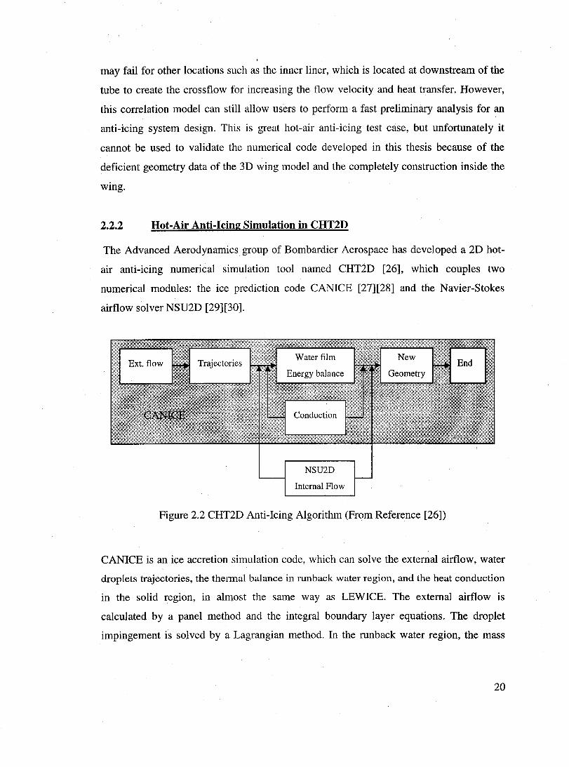
2.2.2 Hot-Air Anti-lcing Simulation in CHT2D
The Advanced Aerodynamics group of Bombardier Aerospace has developed a 2D hot
air anti-icing numerical simulation tool named CHT2D [26], which couples two
numerical modules: the ice prediction code CANICE [27][28] and the Navier-Stokes
airflow solver NSU2D [29] [30].
Water film
NSU2D
InternaI Flow
Figure 2.2 CHT2D Anti-Icing Aigorithm (From Reference [26])
CANICE is an ice accretion simulation code, which can solve the external airflow, water
droplets trajectories, the thermal balance inrunback water region, and the heat conduction
in the solid region, in almost the same way as LEWICE. The external airflow is
calculated by a panel method and the integral boundary layer equations. The droplet
impingement is solved by a Lagrangian method. In the runback water region, the mass
20
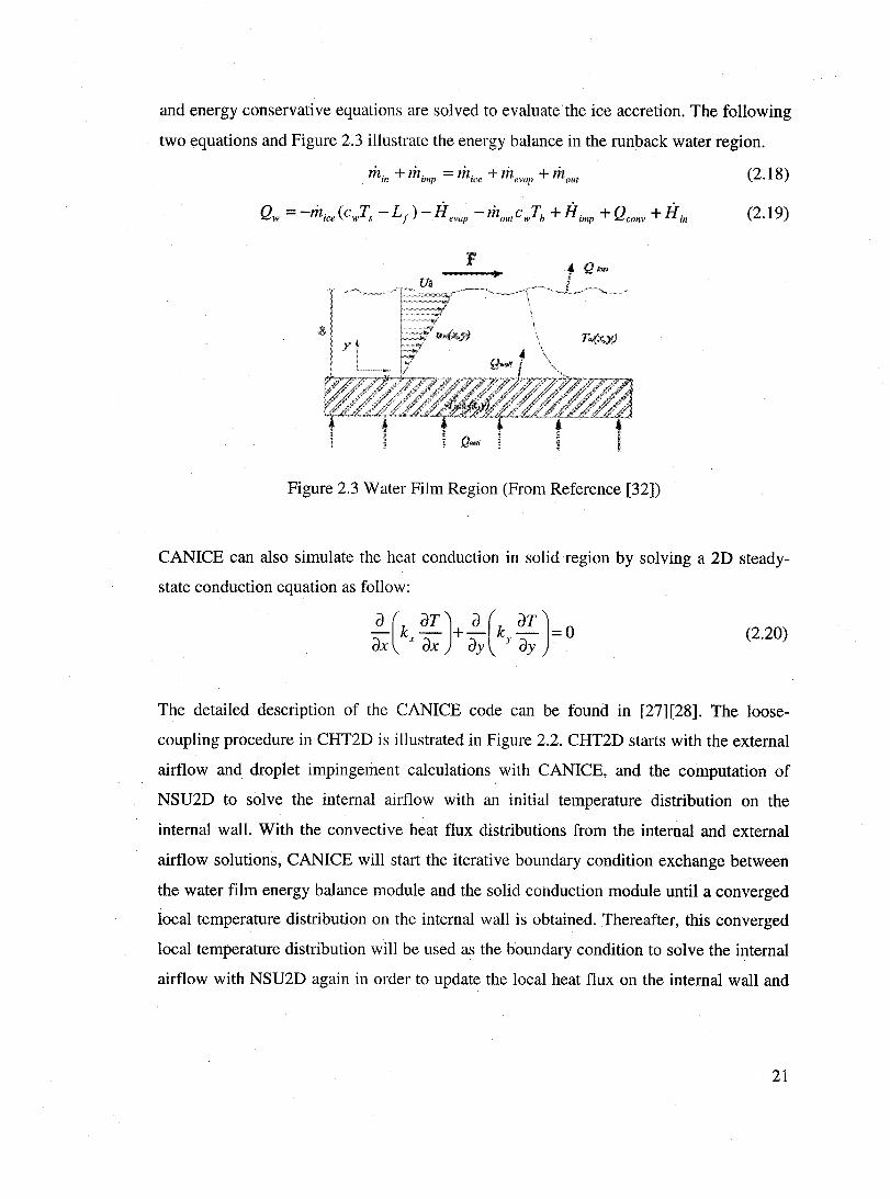
and energy conservative equations are solved to evaluatethe ice accretion. The following
two equations and Figure 2.3 illustrate the energy balance in the runback water region.
(2.18)
(2.19)
1 Q"," , "",1. .. ,,..... r~<~~~"'<-",-< .... ~ ..... ,~
Figure 2.3 Water Film Region (From Reference [32])
CANICE can also simulate the heat conduction in solid region by solving a 2D steady
state conduction equation as follow:
~(k dT)+~(k dT)=O dx x dx dy y dy
(2.20)
The detailed description of the CANICE code can be found in [27][28]. The loose
coupling procedure in CHT2D is illustrated in Figure 2.2. CHT2D starts with the external
airflow and droplet impingement ca1culations with CANICE, and the computation of
NSU2D to solve the internaI airflow with an initial temperature distribution on the
internaI wall. With the convective heat flux distributions from the internaI and external
airflow solutions, CANICE will start the iterative boundary condition exchange between
the water film energy balance module and the solid conduction module until a converged
local temperature distribution on the internaI wall is obtained. Thereafter, this converged
local temperature distribution will be used as the boundary condition to solve the internaI
airflow with NSU2D again in order to update the local heat flux on the internal wall and
21

give it back to CANICE. CHT2D will repeat the two levels of iterations until the
maximum surface temperature variation is lower than O.IK.
Morency et al. [31][32] had performed an anti-icing analysis in CANICE but in their
simulation, the heat flux or heat transfer coefficient distributions had to be imposed on the
internaI surface of the solid region and the internaI jet flow was not solved. Pueyo et al.
[26] have carried out a 2D piccolo tube anti-icing simulation to a wing section of the
Bombardier CRJ700 based on fully CFD-based ca1culations with CHT2D. Three test
cases with dry air conditions has been simulated and compared with wind tunnel
experimental results of the temperature distribution on the external wall. A maximum
temperature difference of rc at the leading edge shows a good agreement between
CHT2D simulations and experimental results. Another test case with icing condition was
also implemented to show the influence ·to the ice accumulation by different anti-icing
heat loads. CHT2D successfully simulated the full range of the anti-icing cases at the
protected region and captured the runback water freezing due to incomplete evaporation.
However, no experimental results for this test case are availablè for validation
The above-mentioned CHT2D code is completely different from the CHT3D code
developed in the present thesis: they do not have any connection except the similarity of
their names.
2.3 Introduction of A Simplified Anti-Icing Experiment
The Laboratoire de Mécanique des Fluides (LMF) of Université Laval has built an
experimental assembly for heat transfer research of aircraft hot-air anti-icing systems [33].
The purpose of their project is to create a database, which can be used to validate anti
icing numerical codes. This experiment is the only one av ail able for validating the hot-air
anti-icing simulation code CHT3D developed in this ,hesis because Laval University
provided detailed information about the experiment, while the detail of any other hot-air
anti-icing experiment is unobtainable due to either the complexity of implementing the
entire hot-air anti-icing experiment or the confidentiality of geometrical or experimental .
data.
22

Thi~ anti-icing system has a hot-air jet flow with 2D properties in order to simplify the
experiment and facilitate the numerical simulation. This experiment assembly is based on
a wind tunnel with a jet generation device below it, and is shown in the following figure.
isolant (phénolique)
débitmètre
1+---900 mm--"';
u~
sortie d'air
montage de --génération du jet
système de chauffage d'air
entrée d'air comprimé
Figure 2.4 The Construction of the Laval University Anti-lcing Experimental Assembly
(From Reference [33])
The test sectibn of the wind tunnel has an inlet with size O.61m by 0.46m. The pressure
gradient on the tunnel floor is similar to the one on the leading edge of a NACA2412
airfoil with a chord length of 2.Sm and an angle of attack of 18 degrees. This pressure
gradient is created by the convergent and divergent shapes of the wind tunnel ceiling. The
wind tunnel floor is comprised of many pieces of aluminum flat plates and one with a
bump surface that can be seen on the figure above. This curve plate is used to simulate the
similar pressure coefficients at an airfoil leading edge. An aluminum flat plate with
150mm in length, 400mm in width and 6.35mm in thickness behind the curve plate is just
located between the wind tunnel airflow and the impinging jet flow. It is isolated from
other parts of the wind tunnel floor by adiabatic materials in order to guarantee that the
heat conduction will not be able to transfer to other parts of wind tunnel floor. The
23

aluminum plate is extended from x/c=O.Ol to x/c=0.07 in the flow direction and is
equipped with Il evenly spaced heat flux gauges. The x is measured from the kink on the
wind tunnel floor and c=2.5m is the chord length of the NACA2412 airfoil. This design
makes the experiment much easier to be implemented than a prototype of a real aircraft
wing. Moreover, to install the measurement equipment on a planar surface is also much
easier than on the curved surface of the wing leading edge.
A slot jet generation device with a rectangular box is installed and fixed just below the
test aluminum plate. The position of jet inlet is 6.35mm lower than the lower surface of
the aluminum plate, which is 4 times the width of the slot jet. The jet is a fully developed
laminar flow at the inlet with a mass flow of 0.004736 kg/s. The jet center is aligned with
the middle point of the aluminum plate located at x/c=0.04.
No water droplets are launched in this experiment, and thus only dry air results are
available. Contrary to most aircraft anti-icing systems, the air at jet nozzle is not choked
and the flow is essentially laminar. This experiment lasted two hours in order to establish
the steady state of surface temperatures.
2.4 Review of Heat Transfer for A Single Siot Jet Impingement
Impinging jets have been widely used in engineering applications, such as aircraft anti
icing systems, turbine blade cooling, and electronic components cooling, due to their high
heatlmass transfer rates. A typical device for the aircraft anti-icing system is the piccolo
tube, which impinges the anti-icing hot air onto the internaI surfaces of protected regions
to prevent the ice buildup on the external surfaces. It's very important to understand the
flow and heat transfer characteristics of impinging jets before performing the numerical
simulation of anti-icing systems.
Figure 2.5 illustrates a single jet flow developing from the nozzle exit with slot width W
or diameter D and impinging on a flat plat surface. This flow pattern can commonly be
divided into three characteristic regions: the free jet region, the stagnation or impinging
region, and the wall jetregion.
24
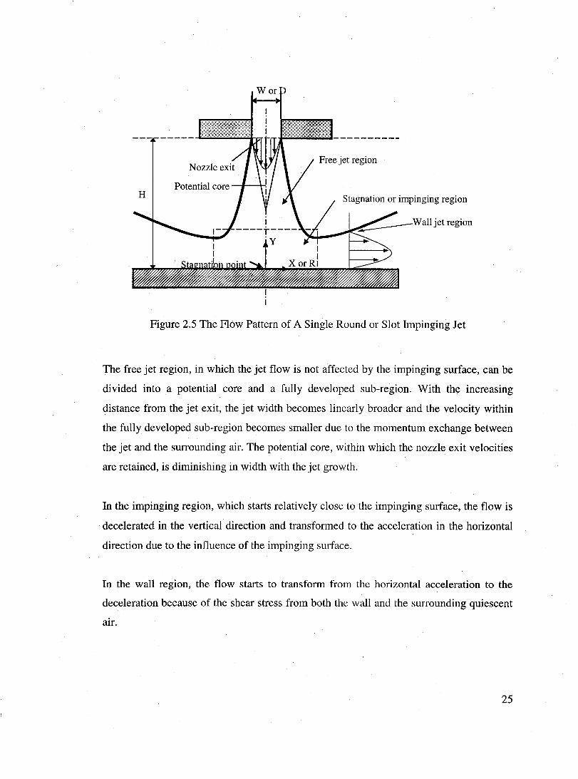
Free jet region
H Stagnation or impinging region
Wall jet region
Figure 2.5 The Flow Pattern of A Single Round or Slot Impinging Jet
The free jet region, in which the jet flow is not affected by the impinging surface, can be
divided into a potential core and a full y developed sub-region. With the increasing
distance from the jet exit, the jet width becomes linearly broader and the velocity within
the fully developed sub-region becomes smaller due to the momentum exchange between
the jet and the surrounding air. The potential core, within which the nozzle exit velocities
are retained, is diminishing in width with the jet growth.
In the impinging region, which starts relatively close to the impinging surface, the flow is
decelerated in the vertical direction and transformed to the acceleration in the horizontal
direction due to the influence of the impinging surface.
In the wall region, the flow starts to transform from the horizontal acceleration to the
deceleration because of the shear stress from both the wall and the surrounding quiescent
air.
25
2.5 Conclusions
As have been discussed above, many algorithms have been developed to solve conjugate
heat transfer problems, which are generally divided into tight-coupling and 100 se
coupling methods. But most of them are developed just for solving dry air heat transfer
problems and only very few numerical codes are able to simulate the hot-air anti-icing
processes. As the complexity of the hot-<;lir anti-icing heat transfer processes, the 100 se
coupling method is always suggested to couple different domains based on an explicit
boundary condition exchange. The objective of this thesis is to develop a CFD-based
conjugate heat transfer procedure, with loose-coupling, to simulate the 3D hot-air anti
icing processes including a 3D external fluid flow, a 3D droplet impingement, a 3D ice
accretion, a 3D heat conduction, and a 3D internaI jet flow. It would be able to simulate a
full range of anti-icing cases and to assist in designing efficient anti-icing systems and in
certifications.
26
CHAPTER 3: Mathematical Equations and
Numerical Methods
The anti-icing simulation procedure developed in this thesis is based on the use orsome
elements of a second-generation 3D in-flight icing state-of-the-art package, FENSAP-ICE,
to iteratively solve the full y 3D viscous fluid flow, the 3D droplet impingement, the 3D
ice accretion, and the 3D heat conduction. This chapter will give a brief introduction of
the mathematical models and numerical methods related to the CRT3D anti-icing
simulations.
3.1 Airflow Model (FENSAP)
FENSAP is a Finite Element Navier-Stokes Analysis Package designed to solve the
steady or unsteady, incompressible or compressible, inviscid or viscous, laminar or
turbulent Newtonian fluid flows by solving the Navier-Stokes equations, the most general
mathematical expression of fluid flows. Accurate evaluation of the convective heat fluxes
at the fluid/structure interfaces from airflow ca1culations is essential for the anti-icing
conjugate heat transfer simulations. The convective heat fluxes are strongly related to the
turbulence models, the rough wall treatment for wet surfaces, and the method of
ca1culating the convective heat fluxes in numerical simulations. Rence, more attention
will be paid to these issues.
3.1.1 Governing Equations
A control volume analysis is used to establish the partial differential governing equations.
Continuity equation:
dp + d(pu;) = 0 dt dx;
(3.1)
Momentum equations: (for Newtonian viscous fluids ignoring the body forces)
27
d(pU;) + d(PU;U;) = _ dp + dru dt dX j dXi dX;
(3.2)
where, ru is the viscous shear stress tensor
ÔU is the Kronecker delta, i.e., ôi; =1 if i=j and ÔU =0 if i;tj.
Energy equation:
The equation of energy conservation follows from the first law of thermodynamics and
states that the total energy of the system has to be conserved.
d(pH - p) + d(pu;H) =~(k~J+ d(uiri;) dt dX j dX j dX j dU;
(3.3)
The left hand side is the change of the total energy in a control volume. The first term in
the right hand side is the heat transfer to the control volume and the second term is the
work done by viscous forces.
For 3D problems, the above 5 governing equations have 9 unknowns, which
arep,u;,uj,uk,p,T,Ji,k,H, hence 4 more equations are required to close the system as
follows.
Ji is the dynamic viscosity of the fluid. For a viscous laminar flow, it can be calculated
from Sutherland's law as:
Ji T T=+110 ( )
3/2( ) Ji= = T= T+ll0
(3.4)
k is the thermal conductivity of the fluid and can also be ca1culated by Sutherland's law
as:
(3.5)
28
The equation of state for an ideal gas:
p=pRT (3.6)
The definition of the total enthalpy:
111-112
Y p H=-V +--2 y-Ip
(3.7)
In FENSAP, the governing equations are non-dimensionalized by introducing the
following dimensionless variables.
x~ =..5.., * =.!!l • p * P T'=~ u; , P = p = [J2' 1 t U~ p~ p= = T~ ,
• JL k*=~ • _ cp H*= H tU= JL =-, C ---. t=--JL~ k~ , l'
cp,~ H= ' t Omitting the star notation, the Navier-Stokes equations can then be rewritten in non
dimensional form as follows:
Continuity equation:
dp + d(pu) =0 dt dX;
(3.8)
Momentum equations:
(3.9)
Energy Equation:
PCpdT d(PCpujT) ( ) 2 Dp 1 d ( dT J (y-l)M 2 d(U;t"J ----'"-+ = y-l M~-+ k- + ~ . (3.10) dt dX j Dt Re ~ Pr~ dX j dX j Re = du j
3.1.2 Numerical Discretization
In FENSAP, the Navier-Stokes equations including the continuity equation, momentum
equations, and energy equation are solved using the weak-Galerkin finite element
discretization scheme. The weak-Galerkin finite element discretization is obtained by
integrating the products of the governing equations in non-dimensional form and the
29
weight functions Wj, which are generally chosen as the shape functions Ni. In FENSAP
solution processes, the continuity equation and momentum equations are first solved in a
coupled way using the weak-Galerkin finite element method to ca1culate the incremental
changes of the primitive variables!1p, !1u1 , !1u2 , !1u3 • The total enthalpy is then solved
from the energy equation using the weak-Galerkin finite element method in term of the
incremental change m . Finally, the variables T, p, f1 ,k are solved from the definition
of total enthalpy, the gas equation of state, and Sutherland's laws.
The linear system of equations is solved using an iterative matrix solver based on the
generalized minimum residual (GMRES) method. For anti-icing simulations in this thesis,
both external and internaI airflows are considered as steady-state problems. In order to
improve the performance of the iterative matrix solver, the steady-state problems are
solved with a local time stepping approach in which the ca1culation starts from the
unsteady-state and advances in time until the steady state of fluid flow is obtained. The
choice of the local time step !1t is based on the stability analysis of the explicit-Euler
centered finite difference scheme, and can be expressed as:
!1t = CFL . !1tstab
!1tstab is the maximum theoretical time step from the stability analysis and varies
according to the element size. Hence, CFL:SI is required for system stability.
In order to overcome the numerical instabilities, artificial viscosity terms are added to the
right hand sides of the continuity, momentum, and energy equations. Different artificial
viscosity schemes have been implemented in FENSAP, such as the Streamline Upwind
(SU) scheme, first order and second order schemes [34].
The fluid energy equation with the weak-Galerkin finite element discretization can be
written as:
(3.11)
30
The thermal boundary conditions have to be defined in the boundary surface integral term
in this discretized energy equation, which is the source term in the finite element
computation. Renee, the thermal boundary conditions on the wall can be either the wall
temperatures Tw or the first derivative of wall temperatures, the convective heat fluxes,
qw = keff ~: • The energy equation calculates temperatures in the entire domain.
3.1.3 Turbulence Models
In FENSAP, the effect of turbulence on the mean flow is modeled using eddy viscosity
models based on Boussinesq's assumption. Th~ Boussinesq assumption states that the
turbulent stress tensor is in the same direction as the laminar stress tensor, thus, aIl
turbulence effects can be represented by an effective viscosity, i.e.
fi Effective = fi La min ar + fiTurbulent
This effective viscosity is then used in the momentum equations. Similarly, the effective
thermal conductivity is defined as:
k F;ffective = k La min ur + kTllrbulent
The turbulent thermal conductivity is estimated from the turbulent viscosity firurbulent and
the turbulent Prandtl number Prt, which is most commonly taken as a constant value of
0.9 in the literature.
k _ C pfiTurbulel1t
Turbulent - P rt
Various turbulence models have been implemented In FENSAP to determine the
turbulent viscosity. They can be divided into one-equation turbulence models such as the
Spalart-Allmaras model and two-equation turbulence models such as. the k-s and k-co
models. The Spaiart-Allmaras and high-Reynolds number k-s turbulence models will be
used in this thesis.
31
3.1.3.1 Spalart-Allmaras Turbulence Model
The Spalart-Allmaras model is a one-equation turbulence model. The turbulent kinematic
viscosity vT is evaluated from a modified viscosity JÏ, which is ca1culated from a non
dimensional transport equation as follows:
d is the distance to the nearest wall.
The magnitude of the modified vorticity is:
- 1 JÏ S = S + ----2-2 IV2
Re~ Je d
The magnitude of the vorticity Sis:
The c10sure functions Iv!' IV2' and Iw are defined as
where,
J, - Z v2 - 1 .vF
+ /Uv!
x = JÏ and v is the laminar viscosity v
The c10sure coefficients are
Ch! =0.1335 Ch2 =0.622 cvl =7.1
Ch! (l+ch2 ) cw! =-2 + cw2 =0.3 cw3 =2
Je cr
('
\ 2
cr=-3
Je = 0.41
Now the modified viscosity can be solved from the transport equation. Hence, the
turbulence kinematic viscosity v T can be determined from the modified viscosity as
32

VT =VfVI
3.1.3.2 k-E Turbulence Model
The k-s model is a two-equation turbulence model, in which the turbulence viscosity is
ca1culated from the turbulence kinetic energy k and its dissipation rate ê as follows:
k 2
PT =pC -f.l IJ
where,
The turbulent kinetic energy k and the dissipation rate ê are solved from their own
transport equations as follows:
dk dk dU; d [( J.LT J dk l P-+PU·-=t'ï--PIJ+- J.L+--I dt .1 dX. .1 dX. dX. (J'k dX. U .1 ] .1 .1
(3.13)
(3.14)
where,
t'.. = 2I1T(S" _.!. dUk g .. J-3. P{(g .. '.1 1"" Il, 3 dX
k U 3 1]
1 (dU. dU i J ' S .. = __ '+_· u 2 dX. dX .
.1 1
The c10sure coefficients are:
CI = 1.44, C2 = 1.92,
For the high-Reynolds model, k and s are only solved from the two transport equations
above beyond the first layer of elements on the wall. In the first layer of elements at the
wall, Reichardt's velocity profile or wall function is applied as follows:
33
u+ =-ln(1+0.4y+ )+7.8 1-exp _L _Lexp(-O.33y+) 1 [( +J + l ./C . 11 11 J
where
TC = 0.41 is the Karman's constant
The definitions of u + and y + are:
+ pyur y =--f1
where y is the normal distance from the nearest wall.
(3.15)
Substituting the above definitions into Reichardt' s velocity profile equation, the friction
velocity Ur can be solved and then used to evaluate the turbulent kinetic energy k and its
dissipation E in the wall elements as follows:
2
k=~ ~Cll '
Then, the values of k and E at the first node off the wall are used as the boundary
conditions of the k-E turbulence equations.
3.1.4 Rough Walls Prediction in Spalart-Allmaras Model
The wall roughness is crucial for accurately predicting the turbulent heat fluxes on a
surface with droplets or ice, which has a large influence on the growth, shape, and type of
ice accretions. Increasing the wall roughness will increase the convective heat transfer,
producing rime ice accretion. In contrast, decreasing the wall roughness will decrease the
convective heat transfer, producing glaze ice accretion. A rough-wall treatment [35] has
been inc1uded in the Spalart-Allamas turbulence model in FENSAP and has proven
successful for icing simulations [36]. For a roughness coefficient ks ' the distance from
the wall used in the turbulence model is increased as:
where d min is the minimum distance from the wall.
As a result, this extension requires a non-zero wall boundary condition for il and a
mixed wall boundary condition:
34
dV V dn d
Many factors may affect the roughness coefficient with complex physical aspects, such as
the velocity, Liquid Water Content (LWC), temperature, droplet diameter, body geometry,
and static pressure. An empirieal correlation is used in FENSAP to evaluate the
equivalent sand grain roughness heightks ' whieh is developed for LEWICE and is
specifically valid for ice accretion [8]. It takes into account the effect of velocity, LWC,
and static temperature and is ca1culated from the following correlation.
k, = [ k,,1 c, l [ k.,1 c, l [ks / c ,1 (k, / c) c S k/ k/ k/ .\ base ( s C )base JV
oo ( s C )hase lwc ( ,\' C )hase J:r,
(3.16)
where
Velocity
[(k k;:) Il ~0.4286+0.0044139(VJ s hase JV
oo
Liquid water content
[(k k;:) ~ ~ 0.5714+ O.2457(LWC) + 1.2571(LWC)' s base JLWC
Statie temperature
[ ks / c ~ = 46.8384(~)-11.2037
(ks / C )base JTs 1000
Baseline value
(ks / C )hase = 0.00117
and c is the characteristic length.
3.1.5 Convective Heat Flux
In the c1assical approach, the surface heat fluxes are ca1culated from the wall temperatlire
gradients. This is, however, a first-order accurate method and needs a very fine mesh in
order to produce an accurate result. A consistent Galerkin finite element approach
developed by Gresho et al. [37] has been implemented in FENSAP to evaluate more
35
accurate surface heat fluxes. This method is used to predict all the convective heat fluxes
in this thesis. The Gresho heat fluxes are second-order accurate and are post-processed
from FENSAP solutions. When the temperatures at the wall are imposed as Dirichlet
boundary conditions, FENSAP evaluates the temperature at all nodes by solving the
weak-Galerkin discretized fluid energy equation as follows:
(3.17)
After obtaining a FENSAP solution, the heat flux at the wall can be evaluated in a reverse
method with the same weak-Galerkin discretized fluid energy equation but replacing the
temperature gradient term in the surface integral by the heat flux as follows:
(3.18)
In this equation, the heat fluxes q at surface nodes are unknown and are solved for. The
volume integral becomes a source term because the temperatures have been solved for by
FENSAP, and are now imposed as boundary conditions. The variable q is only discretized
for the faces at the wall, using 2D shape functions:
m
q = 'LNjqj j=l
3.2 Droplets Impingement Model (DROP 3D)
Supercooled impinging droplets are the cause of in-flight ice accretions. Renee, an
accurate prediction for droplet impingement is crucial for icing/anti-icing/de-icing
36

simulations. DROP3D uses a full Y 3D Eulerian approach, developed by Bourgault et al.
[38] for airflows containing water droplets, as an alternative to the traditional Lagrangian
particle tracking approach for which determining the launching are as for complex 3D
geometries is cumbersome. It computes the droplet velocities and volume fractions of
wa~er at the nodes of the entire computational domain where the airflow variables are
known from airflow solutions. The drop let volume fraction a(x,t) is the mean values of
the ratio of the volume occupied by water over the total volume of the fluid element.
Based on the fact that the icing droplets have a diameter less than lOOllm and a volume
fraction around 10,6, the following assumptions have been used in the DROP3D
mathematical model [38].
• Droplets are spherical without any deformation or breaking;
• No droplet collision, coalescence orsplashing;
• No heat and mass transfer between Jhe droplets and the surrounding air;
• Neglect turbulence effects on droplets;
• The only forces acting on the droplets are drag, gravit y, and buoyancy.
The following non-dimension al droplet continuity and momentum partial differential
equations based on the above assumptions are used to solve the droplet impingement in
DROP3D:
da +V.(aüd)=O dt
(3.19)
aÜd - V- CD Red (- -) (1 Pa J 1 - Pa (dÜa - V-) (3.20) --+u . U = U -u + -- --g+- --+u . u at d d 24K a d P Fr 2 P dt a a
where
Ua Non-dimensional velo city of air
U d Non-dimensional velo city of droplets
P Density of water
Pa Density of air
d Droplets diameter
37

Red Droplet Reynolds number Red = pdU =IÜa -üdl
fi
Fr Froude number Fr=~ .jïi;
K lnertia parameter K=pd2U=
181fi
1 Characteristic length
The drag coefficient CD for spherical droplets depends on the droplet Reynolds number
and is defined as follows:
CD =~(1+0.15Re~·687) for Red ~1300 Red
CD =0.4 for Red >1300
The local collection efficiency /3 is introduced to represent the normalized flux of water
on the aerodynamic surface. It is an important parameter for ice accretion and is post
processed from droplet solutions as follows:
/3=-aud ·n
For a distribution of droplet diameters with Pi as the percentage of droplets in the ith
class, the overall collection efficiency would be:
Then, the water flux at the airfoil surface can be ca1culated as:
mw = L WCU =/3
L WC is the Liquid Water Content and is defined as the ratio of the bulk density of the
drop lets to the bulk density of the air.
A weak-Galerkin finite element method is used to discretize the droplets governing
equations in non-conservative form, and the same Navier-Stokes solver and mesh from
the airflow computation are used. The streamline upwinding (SUPG) terms are added as
stabilization terms to remove possible oscillations in drop let ca1culations.
38
The first two assumptions in the above droplet impingement model are only valid for
droplets with small sizes. However, for Supercooled Large Droplets (SLD), in which the
volume median diameter (MVD) is greater than 50llm, droplet deformation, breakup, and
splashing have to be considered. The SLD model has been recently implemented in
DROP3D by Honsek et al. [39].
3.3 Water FiimlICE Accretion Thermodynamic Model (ICE3D)
ICE3D developed by Beaugendre et al. [40][41][42] is a fully PDE-based 3D ice
accretion model based on the Messenger thermodynamic model [24], in which the
conservation of mass and energy in the water film are defined.
In ICE3D, sorne assumptions are made as follows:
• Small water film thickness, usually less than IOllm;
• Linear velocity profile across the film thickness;
• No air is trapped inside the ice and no air is dissolved in water;
• Shear stress is the main driving force of the water film;
• Constant properties inside the control volume;
• Neglect the conduction between the surface and water;
• Neglect conduction between neighboring control volumes
• Neglect heating of droplets in the air;
• Constant temperature across the water film thickness.
ICE3D requires the solution of the turbulent Navier-Stokes equations and the droplet
solution. The physical thermodynamic model can be expressed in the following general
forrn in a water film control volume:
Mass Balance Equation:
(3.21)
where
39
The rate of change of liquid water within the control volume Ïs:
The mass flux of runback water entering and leaving the control volume is:
The mass flux of incoming water due to impinging droplets is:
The mass flux of water lost due to evaporation/sublimation is:
. r . N (- )d- r· N (- )d-m evap = - J"mevap x,t ,_ x ~ - J,mevap x,t x
The mass flux of water lost due to ice accretion is:
. r . N (- )d-mice = - J, mice X, t x
Energy Balance Equation: . . . . . . .
Qv + QF = Qp + Qevap + Qice + Qconv + Qrad (3.22)
where
The rate of energy change within the control volume is:
The tilde above the T expresses the temperature in degrees Celsius.
The flux of energy lost due to water runback is:
QF = !i!' Pwcp,wT(x,t)üj (x, y,t)'nsdy Yx= i;w !div(hJ.fwallCp,wT(x,t)~x
The flux of incoming energy due to impinging water is:
Q. = rU LWCf3[C T +llüdll211dx p .k = p,w d,= 2
U
40
The flux of energy lost due to evaporation/sublimation is:
Tc = 273.15K is the freezing point of water.
The flux of incoming energy due to ice accretion is:
Qice = lrhice(x,t)[Ljils(TJ-cl'.wf(x,t)~x
The convective heat flux Qconv is calculated from the airflow sol ver and is used to
evaluate the local heat transfer coefficient as follows:
The flux of energy lost due to radiation is:
Qrad = 0"8 IlT~ - (f(x,t)+ TJ4 ~x
or . cr. 4 41.-
Qrad = 0"8 ! L1'= - T px
where 0" is the Boltzman constant and 8 is the emissivity of the solid.
The above mass and energy equations can be expressed in partial differential form with
four compatibility relations as follows:
(3.23)
(3.24)
41

hf ~O
miee ~ ° hfT ~O
miceT ::;; ° (3.25)
In the thermal model above, three unknowns hf,mice , and T are solved from two partial
differential equations. Hence, four compatibility relations are needed to close the system.
These compatibility relations represent the physical observation of water/ice state in
different temperature ranges, and divide them into three icing surfaces as follows:
1. Running wet (no ice) region: T> 0, mice = 0, hf ~o
2. Glaze icing region: T = 0, miee >0 and hf > ° 3. Rime icing region: T < 0, mice ~ ° and hf = °
The physical result must fall into one of these regions and obey the corresponding
compatibility relations. In each region, one variable becomes known and hence, the
system is closed. At each node, the calculation will start at one region, which is
determined by its temperature from the calculation of previous time step. If the new
results obey the compatibility relations of that region, the node will stay in that region,
otherwise it will move to another region until a physical result is obtained.
A finite volume numerical method is used to solve the two partial differential equations
based on a Roe scheme [43][44][45] for spatial discretization and a finite difference
formula is used for time discretization. The two PDEs are solved on the two-dimensional
wall surface in a 3D finite element mesh, the same mesh as that used for the airflow
calculation.
The temperature on the wall T is solved from the energy equation based on the
convective heat flux Qh from airflow solutions and an adiabatic wall boundary condition.
42
3.4 Heat Conduction Model (C3D)
The heat conduction in the solid can be considered as a specific case of the fluid system.
The solid is static and incompressible without volume forces and shear stresses. Therefore,
"the continuity and momentum equations disappear because an the terms go to zero. In the
energy equation, by dropping the null terms, which are the viscous heat dissipation, the
convective term, and the work done by forces, we get the solid conduction governing
equation:
(3.26)
It is also discretized by the weak-Garlerkin finite element method and can be written in
the following non-dimensional form as:
(3.27)
It can also be solved using the same Navier-Stokes solver use for the airflow calculation.
Boundary conditions are needed to make the surface integral term a source term. Either
temperatures (Dirichlet BC) or heat fluxes (Neumann BC) at boundary surfaces have to
be imposed as boundary conditions. Another possible boundary condition is the Robin
boundary condition, in which an artificial parameter, the heat transfer coefficient he ' and a
reference temperature Tref are introduced and are imposed as boundary conditions. Then
the heat flux in the surface integral term (ks dT J is rewritten as he (T - Tref ). The dXi
unknown temperature terms in the surface integral terill are combined with the volume
integral term and the temperatures are solved for by the finite element method.
43

CHAPTER 4: Algorithm for Hot-Air Anti-Icing
Simulation
4.1 General Introduction of Hot-Air Anti-Icing Simulation
When an aircraft flies through clouds or in icy conditions, super-cooled water droplets at
temperatures below the freezing point may impact on aircraft surfaces and result in ice
accretion. For sorne important regions of the aircraft such as wings and nacelles, anti
icing hot air is applied to the internaI surfaces of these regions and the thermal energy is
conducted through the solid body to prevent ice accretion on the external surfaces. The
entire anti-icing heat transfer process for a wing or an engine nacelle can be simply
illustrated in the following figure.
Cold airflow
:
Figure 4.1 The Hot-Air Anti-Icing Heat Transfer Processes
A typical hot-air anti-icing model shown in the figure ab ove has four domains that
correspond to four heat transfer processes. From left to right, they are:
1. External cold airflow domain
44
In this domain, airflow around the airfoil at a temperature lower than the freezing
point of water tends ta freeze the impinging water drop lets on the airfoil external
surface by means of heat convection. The airflow solution including velocities,
heat fluxes, and friction coefficients need to be determined first. The influence to
convective heat flux due to the droplet impingement on the aerodynamic surface is
taken into account by introducing a surface roughness height based on an
equivalent sand grain roughness model, which increases the distance from walls in
the turbulence model.
2. Impinging water film domain
This domain is formed by impinging drop lets. The local collection efficiencies of
impinging droplets on the airfoil are solved by the droplet impingement model
based on the airflow solution. In this domain, the energy balance consists of the
external heat convection, the anti-icing heat conduction, the energy advected by
impinging droplets, the evaporation, the sublimation, the radiation, the water
runback and the ice accretion. The state of the water film in this domain can be
used to indicate the anti-icing effect. The appearance of ice and residual water
indicates an insufficient anti-icing heat flux; conversely, a clean surface indicates
successful, fully evaporative anti-icing. Water runback in this domain is driven by
the viscous force evaluated by the external airflow calculation.
3. Solid conduction domain
The solid domain between the water film and the internaI hot airflow is the
medium through which the internaI hot airflow energy is transferred to the
external surface for anti-icing protection by means of heat conduction.
4. InternaI hot air domain
The internal hot air is bled from the engine compressors and impinges on the front
internaI surface of the airfoil through the holes of piccolo tubes. This internaI
convective heat flux is the source of the anti-icing thermal energy.
45
Hypotheses in hot-air anti-icing simulation:
• The airflow around the airfoil, the droplets impingement, the heat conduction, and
the jet flow inside the airfoil are aIl considered at the steady state. Hence, large
total times are usually chosen for these numerical simulations, especially for the
heat conduction ca1culation, in order to obtain steady-state solutions. The time
marching stepsbetween the coupled domains do not need to be matched.
• The ice accretion process is an unsteady process and the total simulation time
must be specified. In the fully evaporative anti-icing case, it also becomes steady
state.
• The boundary movement of the external surface due to ice accretions is ignored in
anti-icing simulations because a great deal of ice accretion does not occur when
the anti-icing system is engaged.
• The thin film theory makes the following assumptions across the thickness of the
water film:
o Linear velocity profile
o Constant temperature profile
4.2 Overall Energy Balance in the Hot-Air Anti-lcing System
In any anti-icing thermal model, the overall energy conservation of the entire system has
to be guaranteed and the following figure shows aIl of the thermal energy transfer
mechanisms, which are taken into account in this CHT3D model.
46

Runback in
Externai Airflow
convectionD
Radiation
InternaI Jet flow
Runback out
Ice accretion
Figure 4.2 The Overall Energy Balance in the Hot Anti-Icing System
The loose-coupling conjugate heat transfer approach is applied in the hot-air anti-icing
simulation and hence the energy equations in four domains are solved separately and then
are coupled through yxplicit boundary condition exchanges. The heat convection at both
the externai and internaI surfaces of the water/solid system is determined from both the.
externai and internaI airflow calculations through a consistertt Garlerkin FEM post
processing approach developed by Gresho et al. The energy equation of the water filmlice
accretion model is modified with an additional conductive heat flux term for anti-icing
simulations and can be expressed as: . . . . . . . .
Qv + QF = Qp + Qrad + Qevap + Qiee + Qconv + Qcond
This equation indicates that the transfer of the energy in a water film control volume is
caused by water film runback, droplet impingement, radiation, evaporation/sublimation,
ice accretion, and heat conduction from the solid. The equation in partial differential fOfm
is:
47
The heat conduction term is obtained through post-processing of the temperature solution
of conduction through the solid.
The energy equilibrium in the solid domain for steady state can be simply stated that the
total heat flux entering the solid due to the convective heat flux of the internaI jet flow
equals to the total heat flux leaving the solid, which is the conductive heat flux from the
solid to the water film:
The local temperature in the solid is solved from the heat conduction equation in partial
differential form as follows:
(4.2)
4.3 Methodology of Hot-Air Anti-lcing Simulation
The anti-icing model with the above four thermodynamic processes is a special conjugate
heat transfer problem, as it also requires a droplet impingement solution and energy
conservation within the water film. Using the implicit method to solve aIl of these heat
transfer processes simultaneously in the same code is extremely complex. In comparison,
the loose-coupling method has great flexibility to deal with more complicated heat
transfer problems with any number of domains, because each domain is solved
individually with respective sol ver. The loose-coupling method is independent with
regards to the details of each solver and couples the domains by means of exchanging
thermal boundary conditions at common interfaces instead of embedding the solid
conduction, droplet impingement, and ice accretion models into the airflow sol ver. In the
loose-coupling method, aIl of the heat transfer processes are solved sequentially and
iteratively. Another advantage of using a loose-coupling method is the possibility to
directly use the currently available CFD solvers for solving different heat transfer
processes in the hot-air anti-icing model. The CHT3D algorithm is based on a FENSAP
ICE package, which includes the airflow solver FENSAP, the droplet impingement solver
DROP3D, the ice accretion solver ICE3D and the heat conduction solver C3D. "
48
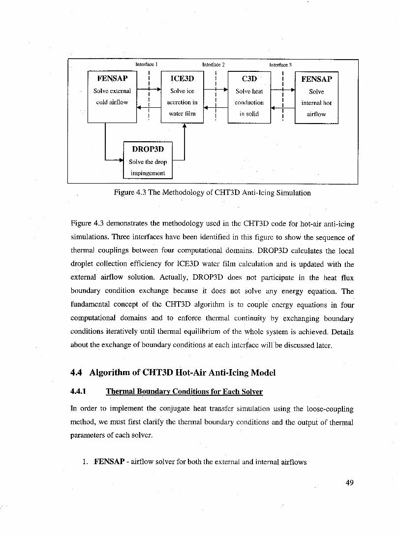
Interface 1 Interface 2 Interface 3
1 1 1 FENSAP 1 ICE3D 1 C3D 1 FENSAP
1 1 1 Solve external
1 Solve ice 1
Solve heat 1
Solve
cold airflow 1 accretion in 1 conduction i internai hot 1 1 1 water film 1 in solid 1 airflow 1 1 1
DROP3D ...
Solve the drop ;--
impingement
Fi~ure 4.3 The Methodology of CHT3D Anti-Icing Simulation
Figure 4.3 demonstrates the methodology used in the CHT3D code for hot-air anti-icing
simulations. Three interfaces have been identified in this figure to show the sequence of
thermal couplings between four computational domains. DROP3D calculates the local
droplet collection efficiency for ICE3D water film calculation and is updated with the
external airflow solution. Actually, DROP3D does not participate in the heat flux
boundary condition exchange because it does not solve any energy equation. The
fundamental concept of the CHT3D algorithm is to couple energy equations in four
computation al domains and to enforce thermal continuity by exchanging boundary
conditions iteratively until thermal equilibrium of the whole system is achieved. Details
about the exchange of boundary conditions at each interface will be discussed later.
4.4 Aigorithm of CHT3D Hot-Air Anti-lcing Model
4.4.1 Thermal Boundary Conditions for Each Solver
In order to implement the conjugate heat transfer simulation using the loose-coupling
method, we must first c1arify the thermal boundary conditions and the output of thermal
parameters of each solver.
1. FENSAP - airflow sol ver for both the external and internaI airflows
49
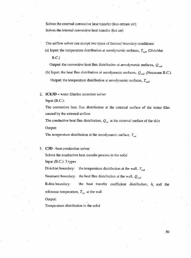
Solves the external convective heat transfer (free-stream air)
Solves the internaI convective heat transfer (hot air)
The airflow sol ver can accept two types of thermal boundary conditions:
(a) Input: the temperature distribution at aerodynamic surfaces, Twall (Dirichlet
B.C.)
Output: the convective heat flux distribution at aerodynamic surfaces, Qwall
(b) Input: the heat flux distribution at aerodynamic surfaces, Qwall (Neumann B.C.)
Output: the temperature distribution at aerodynamic surfaces, Twall
2. ICE3D - water film/ice accretion solver
Input (B.C.):
The convective heat flux distribution at the external surface of the water film
caused by the external airflow
The conductive heat flux distribution, Qext at the external surface of the skin
Output:
The temperature distribution at the aerodynamic surface, Tex!
3. C3D - heat conduction solver
Solves the conductive heat transfer process in the solid
Input (B.C.): 3 types
Dirichlet boundary: the temperature distribution at the wall, Twall
Neumann boundary: the heat flux distribution at the wall, Qwall
Robin boundary: the heat transfer coefficient distribution, he and the
reference temperature, Trel at the wall
Output:
Temperature distribution in the solid
50
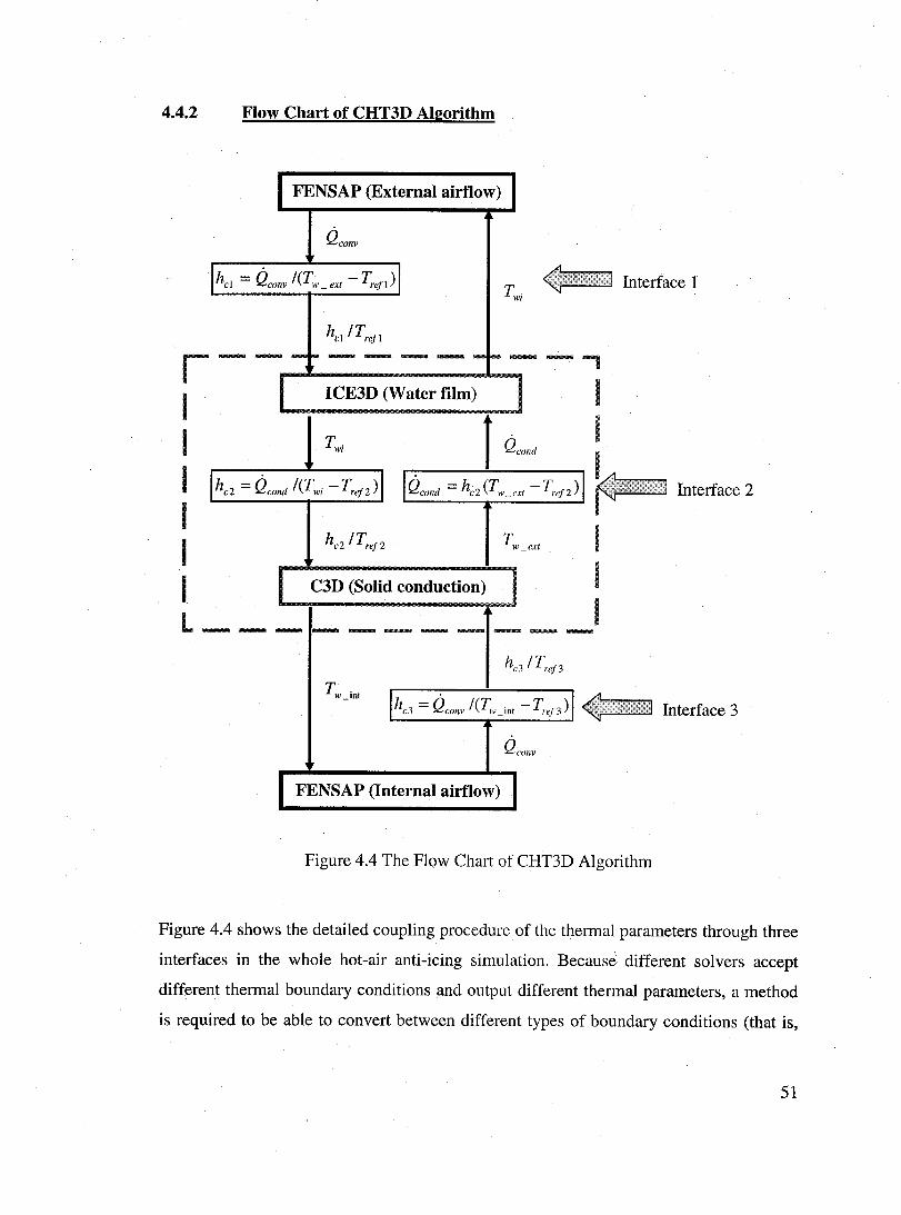
4.4.2 Flow Chart of CHT3D Aigorithm
FENSAP (External airflow)
Qconv
hel = Qconv /(T;, _ ext - Tren ) Interface 1
r -- -11""""'&...---"""""' ............ ---........... - ........ .......,. ......... -- ,
1 ICE3D (Water film) 1
1 T~ l Q"'M :
1 h" = Q_ I(T wi - T ref2 ) Q"md = he> (Tw "" m - T'if2) rlinLC1
1 1 hc2/Tref2 T w_ ext 1
1 C3D (Solid conduc . 1 1 L ________ ~ __
Interface 2
Qconv
FENSAP (Internai airflow)
Figure 4.4 The Flow Chart of CHT3D Algorithm
Figure 4.4 shows the detailed coupling procedure of the thermal parameters through three
interfaces in the whole hot-air anti-icing simulation. Because different solvers accept
different thermal boundary conditions and output different thermal parameters, a method
is required to be able to convert between different types of boundary conditions (that is,
51

temperatures or heat fluxes). In CHT3D, a local heat transfer coefficient he and a
reference temperature Trel are defined at each interface in order to implement these
conversions.
he = Qw /(Tw - Tr~l)
Qw = he (Tw - Tr~l)
(4.3)
(4.4)
(4.5)
The reference temperature at each interface is defined at the beginning of a CHT3D
ca1culation and is fixed for all CHT3D ca1culation cycles. The reference temperature Trel
at each interface must be carefully chosen to avoid Tw = Trel during the CHT ca1culation.
The standard choice is either the mainstream airflow temperature or the local wall
temperature calculated by the airflow solver based on an adiabatic boundary condition.
Equation (4.3) is used to evaluate the heat transfer coefficient distribution from the known
temperature Tw and heat flux Qw distributions at each interface. The ca1culation of the
heat transfer coefficient he distribution at each interface is updated in each corresponding
iteration. Equations (4.4) and (4.5) are used to convert between the temperature
distribution and the heat flux distribution at each interface based on the distribution of the
heat transfer coefficient he'
4.4.3 Boundary Condition Exchange at Each Interface
In Figure 4.4, four computational domains are separated by three interfaces. From top to
bottom, they are:
1. Interface 1 between the external cold airflow and the water film.
This interface is used to couple and exchange boundary conditions between the
external airflow solver, FENSAP, and the ice accretion solver, ICE3D. The
reference temperature at this interface is chosen as the free stream tempe rature of
52
the external cold airflow, Trefl = T=. The external airflow solver, FENSAP, uses
the local wall temperature Twi ca1culated by ICE3D as the Dirichlet thermal
boundary condition, Tw_ ext = Twi to compute the local convective heat flux at
interface 1. The local convective heat flux from the FENSAP solution will be used
to ca1culate the new local heat transfer coefficient from the following equation,
and is used with the reference temperature Tren as the Robin boundary condition
for ICE3D.
(4.6)
2. Interface 2 between the water film and the solid
This interface is used to couple and exchange boundary conditions between the ice
accretion solver, ICE3D and the solid conduction solver, C3D. The reference
temperature in this interface is also defined as the free stream temperature of the
external cold airflow, Tr~f2 = T=. The local temperature T w_ext on the solid
external surface from the C3D ca1culation will be converted to a local conductive
heat flux as the Neumann boundary condition of ICE3D using the following
equation.
(4.7)
The local heat transfer coefficient hc2 in this equation is obtained from the
previous iteration. The local wall temperature Twi ca1culated by ICE3D is used to
ca1culate the new local heat transfer coefficient at interface 2 and is used
afterwards with the reference temperature Tref2 as the Robin boundary condition
at the solid external surface for the C3D conduction ca1culation. The new local
heat transfer coefficient is ca1culated by the following equation:
(4.8 )
3. Interface 3 between the solid and the internaI hot airflow
53
This interface is used to couple and exchange boundary conditions between the
solid conduction solver, C3D, and the internaI airflow sol ver, FEANSAP. The
local reference temperature Tref3 is the local wall temperature obtained by solving
the internaI airflow with an adiabatic wall boundary condition. The local
temperature on the solid internaI surface from the C3D solution is used as the
Dirichlet thermal boundary condition for the internaI hot airflow caIculation. The
internaI airflow solver, FENSAP, calculates the local convective heat flux at this
interface, which is used to caIculate a new local heat transfer coefficient by the
following equation.
(4.9 )
This local heat transfer coefficient will be used with the local reference
temperature Tref3 as the Robin boundary condition at the solid internaI surface for
the solid conduction caIculation.
4.4.4 Implementation of Hot-Air Anti-Icing Simulation in CHT3D
Following the introduction of the coupling methods at each interface? we will discuss how
the CHT3D works and couples the entire system to carry out the anti-icing simulation. AlI
discussions will still refer to Figure 4.4. In order to start the CHT3D simulation, initial
thermal boundary conditions must be assumed at each interface. Initial wall temperatures
are guessed for both interface 1 and interface 3 and an initial conductive heat flux is
guessed for interface 2. After that, CHT3D will start the caIculation as follows:
1. Solve the internaI airflow using FENSAP by imposing an adiabatic boundary
condition at interface 3 to caIculate the reference temperature distribution at
interface 3, Tref3 •
2. Solve the external airflow using FENSAP with the boundary condition of the
temperature distribution at interface 1 to obtain a heat flux distribution at
interface .
54
3. Evaluate the heat transfer coefficient distribution based on the temperature and
heat flux distributions at interface 1 and prepare the Robin boundary condition for
ICE3D at interface 1.
4. Solve the internaI airflow using FENSAP with the boundary condition of the
temperature distribution at interface 3 to obtain a heat flux distribution at interface
3.
5. Evaluate the heat transfer coefficient distribution based on the temperature and
heat flux distributions at interface 3 and prepare the Robin boundary condition for
C3D at interface 3.
6. ICE3D ca1culates the temperature distribution at interface 2 with the Robin
boundary condition at interface 1 and the conductive heat flux distribution Qcond
at interface 2.
7. The heat transfer coefficient distribution at interface 2 is evaluated based on the
temperature and heat flux distributions and pass a Robin boundary condition to
C3D at interface 2.
8. C3D caIculates the temperature distribution in the solid with Robin boundary
conditions at interface 2 and interface 3 and evaluates the temperature
distributions at interface 2 and interface 3.
9. Convert the temperature distribution at interface 2 to a heat flux distribution and
pass it to ICE3D.
10. ICE3D and C3D start an inner loop by iteratively exchanging boundary conditions
to each other at interface 2. Steps 6 to 9 are repeated until partial convergence is
achieved or until a specifie number of iterations of the inner loop have been
completed.
Il. ICE3D outputs the temperature distribution at interface 1 and passes it to. the
external airflow solver FENSAP, and C3D outputs the temperature distribution at
interface 3 and passes it to the internaI aÏl'flow solver FENSAP.
12. Both the externaI and the internaI FENSAP calculations are updated based on the
upqated Dirichlet boundary conditions at interface 1 and interface 3. CHT3D
repeats steps 2 to Il above until the temperature distribution at each interface is
converged.
55

4.4.5 Dual Surface Meshes
In thermal boundary conditions, the temperature is base on finite element nodes, but the
heat flux and the heat transfer coefficient are based on surface cells, so the exchange of
heat fluxes or heat transfer coefficients at each interface cannot be directly implemented.
The heat transfer coefficient can also not be directly ca1culated from the face-based heat
flux and the node-based temperature. A dual surface mesh is çreated at each interface to
convert the values of heat fluxes or heat transfer coefficients from surface cells to finite
element nodes before passing them at interfaces or converting them from finite element
nodes to surface cells after passing them at interfaces. The dual meshes scheme was
developed by Beaugendre and was implemented in the icing accretion simulation [42].
The dual surface mesh is obtained from the surface mesh by connecting each cell centroid
to the midpoints of cell edges. The following figure shows an example of the dual meshes
on a structured grid.
1 1
: A2 BI 1 B2 Al'I
~~---- ------. -----...,., ~ -j-----1 1
A3
1 1 1
A4
Dl ~ D2 _----.r;---
1 1
1 D4
B3
Cl C2 -----.i{-
1
C3 : C4 1 1
Surface mesh
Dual surface mesh
Figure 4.5 Dual Meshes on Structured Grid
Four surface cells, named A, B, C, and D, are drawn with solid lines in the figure above
and l, J, K, and L are the corresponding centroids of these cells. Dual surface meshes are
drawn with dash lines such as the dual surface mesh cell DKL. The average heat flux or
heat transfer coefficient over each cell of the dual surface mesh is evaluated and is then
set at the corresponding node of the surface mesh. For ex ample, the average heat flux or
56
heat transfer coefficient over the dual surface mesh cell IJKL will be set to the node M.
The energy conservation has to be guaranteed for each surface eell when converting heat
fluxes or heat transfer coefficients from surface cells to nodes. For example, the following
relationship is used to ca1culate the heat flux at node M from the values on surrounding
cells A, B, C, and D to ensure that the heat flow rate through the surface UKL is
conservative.
Hence,
Q _ QI SA4 +Q]SB3 +QKSCI +QLSD2
M - (SA4 +SB3 +SCI +SD2) (4.10)
The same method is used to convert the face-based variables in the opposite way from
nodes to cells.
4.4.6 Boundary Condition Exchange for Matching and Non-Matching Grids
In the current CHT3D code, the transfer of the thermal parameters at the common
interfaces between different domains is only applicable for matching grids, which allows
the direct transfer of parameters node-to-node and hence is more conservative and
accurate than non-matching grids. But the mesh generation for matching grids is
sometimes challenging, especially for industrial-level applications with complex 3D
geometries, because the grids of different domains have to be generated at the same time
and only structured grids can be used to guarantee that the nodes match at the common
interfaces.
The non-matching grids are easier to generate because unstructured grids can be used and
the grids of different domains can be generated separately. In addition, it is common to
user a much finer mesh for a fluid domain than a solid domain. Henee, boundary
condition exchange for non-matching grids can increase the flexibility of the CHT
application and take advantage of mesh adaptation for fluid ca1culations, which is more
efficient for unstructured meshes. However, it does not improve the quality of the
CHT3D coupling procedure.
57
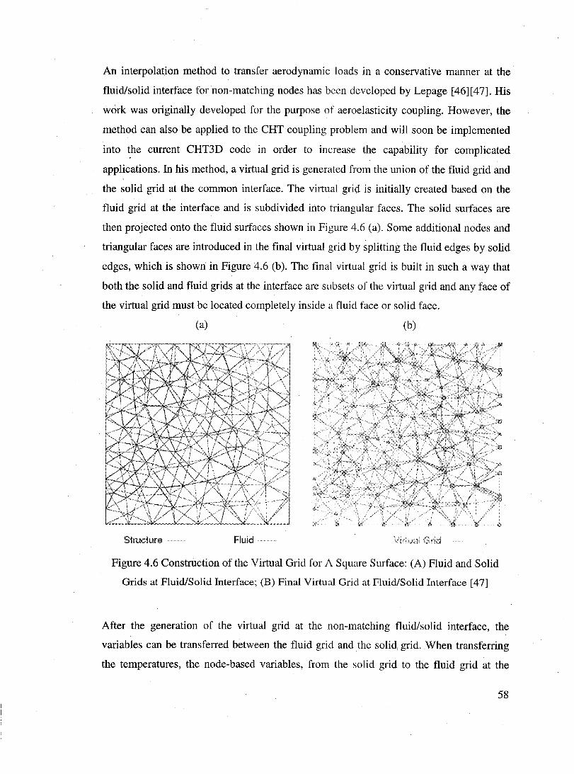
An interpolation method to transfer aerodynamic loads in a conservative manner at the
fluid/solid interface for non-matching nodes has been developed by Lepage [46][47]. His
work was originally developed for the purpose of aeroelasticity coupling. However, the
method can also be applied to the CHT coupling problem and will soon be implemented
into the current CHT3D code in order to increase the capability for complicated
applications. In his method, a virtual grid is generated from the union of the fluid grid and
the solid grid at the common interface. The virtual grid is initially created based on the
fluid grid at the interface and is subdivided into triangular faces. The solid surfaces are
then projected onto the fluid surfaces shown in Figure 4.6 Ca). Sorne addition al nodes and
triangular faces are introduced in the final virtual grid by splitting the fluid edges by solid
edges, which is shown in Figure 4.6 Cb). The final virtual grid is built in such a way that
both the solid and fluid grids at the interface are subsets of the virtual grid and any face of
the virtual grid must be located completely inside a fluid face or solid face.
Ca) Cb)
S1 ruc1 ure Fluid ...
Figure 4.6 Construction of the Virtual Grid for A Square Surface: CA) Fluid and Solid
Grids at Fluid/Solid Interface; (B) Final Virtual Grid at Fluid/Solid Interface [47]
After the generation of the virtual grid at the non-matching fluid/solid interface, the
variables can be transferred between the fluid grid and the solid grid. When transferring
the temperatures, the node-based variables, from the solid grid to the fluid grid at the
58

interface, the temperatures at the nodes of the solid surface are first transferred to the
matching nodes on the virtual grid. Then the temperatures on the other nodes of the
virtual grid cao be evaluated using linear interpolation over the triangular faces. FinaIly,
the temperatures of the fluid nodes at the interface can be directly transferred from the
matching nodes of the virtual grid because the temperatures at aIl the nodes of the virtual
grid have already been evaluated.
However, when transferring the face-based variables, such as the heat fluxes, special
attention has to be paid to ensure the transfer is in a conservative form. For transferring
the heat flux from the fluid grid to the solid grid at the fluidlsolid interface, the face-based
heat fluxes at the fluid surface are first transferred to the corresponding faces of the
virtual grid. Then, the heat balance across the CHT interface has to be conservative, i.e.
the total heat flow though the solid surface must equal to the total heat flow through the
fluid surface. It can be expressed as:
r q dA = "r qfv, dA JI\(S) ,\' .L.J JA(e)
vcS
(4.11)
This equation represents the local heat flux conservation for each solid face and can be
more easily understood from the following figure, which shows that the heat flow though
a solid face equals the total heat flow through a1J the virtual faces inside the solid face.
Hence, global conservation is automatically satisfied.
Figure 4.7 Evaluation of A Surface Integral on the Virtual Grid [47]: the Red Triangle Is
A Solid Face and Blue Triangles Are Fluid Faces.
59
Since the heat fluxes are considered as constant over each fluid face and each solid face,
the above integral equation for each solid face can be simplified as:
qsA(S) = Lq;A(V) vcS
Then, the heat flux though the solid face can be caIculated as follow:
Lq;A(V)
q _ -"-,vc",,s~::-:--_ S - A(S)
4.4.7 The Stability Analysis of Conjugate Heat Transfer Anti-Icing Simulation
A common problem for the loose-coupling approach is the stability of the calculation.
Giles[13] has studied the stability of the loose-coupling approach for computing the
temperatures and the heat fluxes in coupled fluid/structure interactions. From his study,
using a Neumann boundary condition for the structure calculation and a Dirichlet
boundary condition for the fluid calculation are suggested to achieve numerical stability.
The reverse will cause numerical instability. Most of the CHT codes use a relaxation
parameter to relax the local temperature on the solidlfluid interface before imposing it as
the boundary condition to an airflow calculation because the fluid flow calculation is very
sensitive to the boundary condition changes. This relaxation can be expressed in the
following equation.
T n+l = T n+1 (1- fJ) + flTn new
A higher value of the relaxation parameter fJ ' within the range of [0, 1] corresponds to a
higher relaxation. This method is an explicit method to reduce the instability of the
system but also greatly increases the computing time. Usually, a relaxation scheme should
be used in this method so that the initial relaxation is higher and less relaxation is
subsequently used to increase the convergence speed. Extra efforts must be paid to find a
proper relaxation scheme. Another method, which is used in the CHT3D simulation to
relax the boundary condition exchange to the t10w solver, is to impose the Robin
boundary conditions to the structure conduction code instead of directly imposing the
Neumann boundary conditions. In this method, a virtual heat transfer coefficient variable
is introduced and is converted from the convective heat t1ux as has been discussed in
section 4.4.3. The heat transfer coefficients are used in both interface 1 and interface 3
60

and are ca1culated using the equation he = Q ICT - Tret ) . In this implicit relaxation method,
the relaxation is automatically adjusted according to the deviation of the heat flux from
the final converged result. In addition, reducing the time step and iteration numbers in
each domain's ca1culation and increasing the total number of coupling loops of CHT3D
will make the CHT3Dcoupling tighter and hence increase the stability of the ca1culation.
Moreover, in the CHT3D algorithm, more frequent coupling between ICE3D and C3D in
the inner loop will cause higher relaxation in the inner loop outputs, the temperature
distributions at both interface 1 and interface 3 and will increase the stability of the
CHT3D ca1culation as a result.
4.5 Conclusions
A loose-coupling conjugate heat transfer model, CHT3D, based on explicit boundary
condition exchange has been developed to simulate the 3D heat transfer processes of
aircraft hot air anti-icing systems. This model uses a modular approach and couples the
external airflow domain, water film/ice accretion domain, solid conduction domain, and
internaI airflow domain, with currently available numerical solvers, FENSAP-ICE
package. The temperature and heat flux distributions at each coupling interface are
calculated and the anti-icing effect can be evaluated from the solution of the watyr film
domain. This approach can also simulate any conjugate heat transfer problem with two
different fluid domains and one solid conduction domain and can be easily expended to
applications with any number of fluid/solid interfaces. The solver of each domain in the
modular approach can be upgraded independently and separately. In the airflow solver, a
more accurate local convective heat flux at the boundary surface, the so-called Gresho
heatflux, is ca1culated with a consistent weak Garlerkin FEM post-processor instead of
the classical method of temperature differences. A sand grain roughness model is used to
model the surface roughness due to the drop let impingement, which has a significant
impact to the convective heat flux at the surface. The different turbulence models in the
airflow solver may be required for different types of airflows in order to predict the
accurate convective heat fluxes at the fluidlsolid interface. The verification and validation
of the CHT3D model will be presented in the following chapters.
61
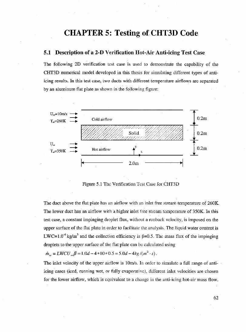
CHAPTER 5: Testing ofCHT3D Code
5.1 Description of a 2-D Verification Hot-Air Anti-icing Test Case
The following 2D verification test case is used to demonstrate the capability of the
CHT3D numerical model developed in this thesis for simulating different types of anti
icing results. In this test case, two ducts with different temperature airflows are separated
by an aluminum flat plate as shown in the following figure:
Uoo=lOmls ----. ----. Cold airflow 0.2m Too=260K ----.
0.2m
Uoo ----. ----. Hot airflow f ~x 0.2m Too=35OK ----.
I~ 2.0m ~I
Figure 5.1 The Verification Test Case for CHT3D
The duct above the flat plate has an airflow with an inlet free stream temperature of 260K.
The lower duct has an airflow with a higher inlet free stream temperature of 350K. In this
test case, a constant impinging droplet flux, without a runback velocity, is imposed on the
upper surface of the flat plate in order to facilitate the analysis. The liquid water content is
LWC=1.0-4 kg/m3 and the collection efficiency is ~=0.5. The mass flux of the impinging
droplets to the upper surface of the flat plate can be ca1culated using
mw = LWCU ~f3 = 1.0d -4* 10*0.5 = 5.0d -4kg /(m 2 . s).
The inlet velocity of the upper airflow is lOmls. In order to simulate a full range of anti
icing cases (iced, running wet, or fully evaporative), different inlet velocities are chosen
for the lower airflow, which is equivalent to a change in the anti-icing hot-air mass flow.
62

AlI of the results are plotted for -O.5m < x < O.5m along the length of the aluminum flat
plate.
This test case is designed for testing the functioning of the CHT3D code without
comparing it to any experimental or numerical results. Therefore, only the coarser meshes
are used in order to reduce the computational expense involved. This 2D test case is
simulated using 3D meshes with 2 nodes in the' z-direction and a periodic condition
imposed on the two surfaces perpendicular to the z-axis.
5.2 Hot-Air Anti-lcing Simulations
5.2.1 Case 1: Hot-Air Anti-Icing Simulation with Ice Accretion
With the inlet velocity of the lower hot airflow at 5m/s, the anti-icing thermal energy is
not enough to prevent the ice accretion on the entire upper surface of the aluminum flat
plate. The iced anti-icing results obtained from CHT3D calculation are shawn below.
0.0007
0.0008
0.0005
0.0004
0.0003
0.0002
0.0001
IMP INGING Fl..üW
-0.4 -0.2
MASSOF ICE
MASS OFFLM
a 0.2 0.4
POSITION ON THE PLATE -- X (ml
Figure 5.2 Water Film Mass Flow on
Upper Surface of the Flat Plate
1200 CONVECTION
1100
cr·, 1000 <? -
~ ~ 900 -X =, ..J 800 li.
~ w 700 I -600
500 -0.4 -0.2 a 0.2 0.4
POSITION ON THE PLATE -- X (ml
Figure 5.3 Heat Flux Distribution on Upper
Surface of the Flat Plate
63

275.5
275
g w
274.5 cr: F cC cr: w 274 a. :! ~
273.5
273 ·0.4 ·0.2 0 0.2 0.4
POSITION ON THE PLATE·· X (m)
Figure 5.4 Temperature Distribution on ( .
Both Surfaces of the Flat Plate
In the range from x=-O.5m to x=-O.04m on the upper surface of the aluminum flat plate,
the wall temperature decreases from 273.7K to 273.15K and no ice accretion is predicted.
However, the anti-icing heat flux is not enough to evaporate aIl the impinging water; thus,
the residual water film on the upper surface of the flat plate is still present. Thedecrease
of the evaporative water flux in the airflow direction is due to a decrease of the surface
temperatures.
In the range from x=-O.04m to x=O.5m, the wall temperature on the upper surface
becomes constant and equal to the freezing point 273.15K. As a result, the coexistence of
the ice and the water film is present on ,the upper surface. The increase of the
instantaneous mass of ice along the airflow direction is a result of a decrease of the anti
icing hot-air thermal energy. The mass flux of the evaporative water is almost constant
because it primarily depends on the surface temperatures. The residual water film on the
upper surface decreases due to an increase of ice.
The mass flow figure indicates the mass conservation of the water film. The sum of the
evaporative mass flux, ice accretion mass flux, and the instantaneous mass of residual
water on the upper surface of the fIat plate equals the mass flux of the impinging droplet.
64
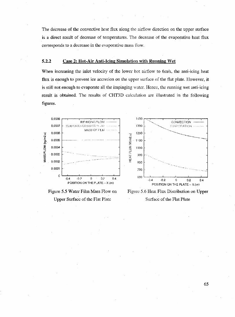
The decrease of the convective heat flux along the airflow direction on the upper surface
is a direct result of decrease of temperatures. The decrease of the evaporative heat flux
corresponds to a decrease in the evaporative mass f1ow.
5.2.2 Case 2: Hot-Air Anti-Icing Simulation with Running Wet
When increasing the inlet velocity of the lower hot airflow to 6m/s, the anti-icing heat
flux is enough to prevent ice accretion on the upper surface of the flat plate. Rowever, it
is still not enough to evaporate all the impinging water. Renee, the running wet anti-icing
result is obtained. The results of CRT3D calculation are illustrated in the following
figures.
~ Ç\J
~ <$
~ ...J u.
~ ~
0.0008 IMP ING ING FLOVIJ
0.0007 MASS OF FiLM
O.OOOS
0.0005
0.0004
0.0003
0.0002
0.0001
0 ·0.4 ·0.2 o 0.2 0.4
POSITION ON THE PLATE -- X (m)
Figure 5.5 Water Film Mass Flow on
Upper Surface of the Flat Plate
1400 CONVECTIOf\J
1300
~~ 1200 "
~ 1100 ~ ... X 1000 :::J ...J LL
~ 900 w I 800
700
-0.4 -0.2 0 0.2 0.4
POSITION ON THE PLATE·· X (m)
Figure 5.6 Reat Flux Distribution on Upper
Surface of the Flat Plate
65
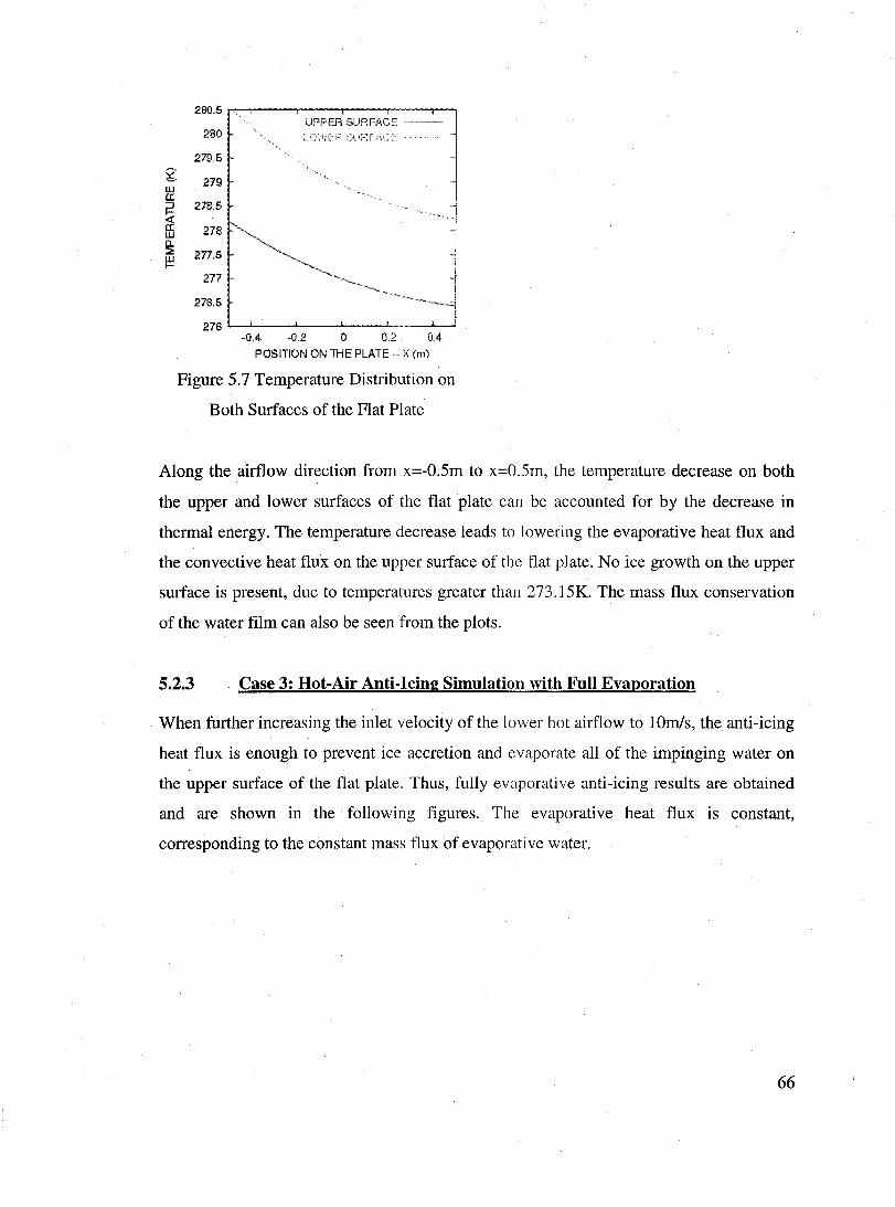
g w 0:
~ <t: 0: w ~ ~
280.5 UPPER SURFIICE
280
279.5
279
278.5
278
277.5
277
276.5
276 -0.4 -0.2 o 0.2 0.4
POSITION ON THE PLATE --)( (ml
Figure 5.7 Temperature Distribution on
Both Surfaces of the Flat Plate
Along the airflow direction from x=-O.5m to x=O.5m, the temperature decrease on both
the upper and lower surfaces of the flat plate can be accounted for by the decrease in
thermal energy. The temperature decrease leads to lowering the evaporative heat flux and
the convective heat flux on the upper surface of the fIat plate_ No ice growth on the upper
surface is present, due to temperatures greater th an 273.15K. The mass flux conservation
of the water film can also be seen from the plots.
5.2.3 Case 3: Hot-Air Anti-Icing Simulation with Full Evaporation
When further increasing the inlet velocity of the lower hot airflow to lOmfs, the anti-icing
heat flux is enough to prevent ice accretion and evaporate aIl of the impinging water on
the upper surface of the flat plate. Thus, fully evaporative anti-icing results are obtained
and are shown in the following figures. The evaporative heat flux is constant,
corresponding to the constant mass flux of evaporative water.
66

ut oN
i ~ 0 -l IL
~ ::!:
0.000506 IMPiNGING FLOW
0.000504
0.000502
0.0005
0.000498
0.000496
-0.4 -0.2 o 0.2 0.4
POSITION ON THE PLATE -- X (m)
Figure 5.8 Water Film Mass Flow on
Upper Surface of the Flat Plate
296 UFPEFl sunFAC['
295
g 294 w cc 293 :J t-~
292 w 9: ~ 291
290
289 -0.4 -0.2 o 0.2 0.4
POSITION ON THE PLATE -- X (111)
Figure 5.10 Temperature Distribution on
Both Surfaces of the Flat Plate
2600
2400
U) 2200 ~ ~- 2000 x :J ....1 leoo IL
t;ï; w 1600 I
1400
1200 -0.4 -0.2 o 0.2 0.4
POSrrlON ON THE PLATE -- X (m)
Figure 5.9 Heat Flux Distribution on Upper
Surface of the Flat Plate
5.2.4 Case 4: Hot-Air Anti-Icing Simulation Without Droplets Impingement
Another test case is also performed with the same inlet velocity of the hot airflow as the
above full y evaporative case (10 mis), but without impinging water, in order to observe
the influence of the impinging water. The following figures show that the temperatures
and heat fluxes further increase on the flat plate surfaces because the hot-air energy is just
used to heat up the solid temperatures without any Joss to water evaporation.
67
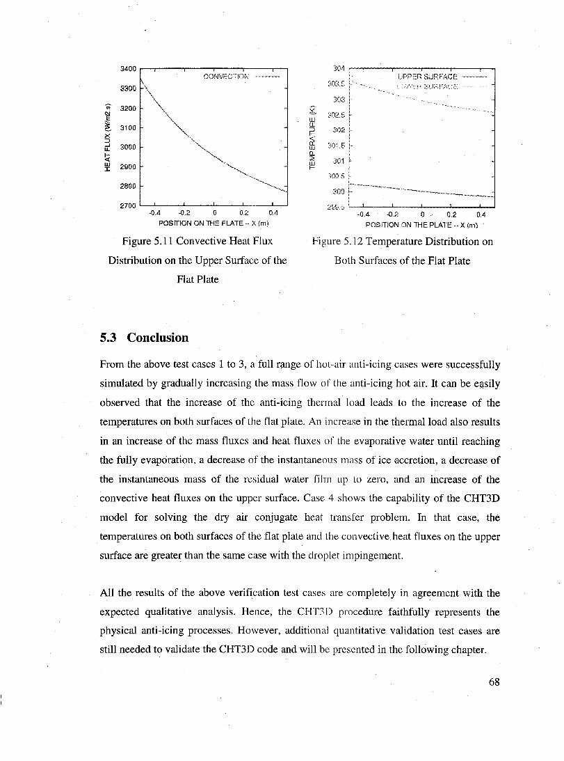
3400 CONVECllCJr~
3300
~ 3200 ~ ! 3100 x ::J ...J 3000 LI.
~ w 2900 ::x;
2800
2700 '--...1..-_--' __ -'-_---''--_-'----'
-0.4 -0.2 0 0.2 0.4
POSrrlON ON THE PLATE -- X (m)
Figure 5.11 Convective Heat Flux
Distribution on the Upper Surface of the
Flat Plate
5.3 Conclusion
304
~i03.5 ""
303 g
é~02.5 w ([
:::J 302 1-<t: cc :,:015 w CL :2 :{01 w 1-
:;005
300
2P9.S -0.4 -0.2 o ~ 0.2 0.4
POSITION ON THE PLATE -- X (111)
Figure 5.12 Temperature Distribution on
Both Surfaces of the Flat Plate
From the above test cases 1 to 3, a full range of hot-air anti-icing cases were successfully
simulated by gradually increasing the mass flow of the anti-icing hot air. It can be e;;tsily
observed that the increase of the anti-icing thermal load leads to the increase of the
temperatures on both surfaces of the flat plate. An increase in the thermalload also results
in an increase of the mass fluxes and heat fluxes of the evaporative water until reaching
the fully evaporation, a decrease of the instantaneous mass of ice accretion, a decrease of
the instantaneous mass of the residual water film up to zero, and an increase of the
convective heat fluxes on the upper surface. Case 4 shows the capability of the CHT3D
model for solving the dry air conjugate heat transfer problem. In that case, the
temperatures on both surfaces of the flat plate and the convective heat fluxes on the upper
surface are greater than the same case with the drop let impingement.
AIl the results of the above verification test cases are completely in agreement with the
expected qualitative analysis. Hence, the CHT3D procedure faithfully represents the
physical anti-icing processes. However, addition al quantitative validation test cases are
still needed to validate the CHT3D code and will be presented in the following chapter.
68
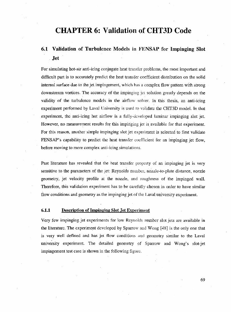
CHAPTER '6: Validation of CHT3D Code
6.1 Validation of Turbulence Models III FENSAP for Impinging Siot
Jet
For simulating hot-air anti-icing conjugate heat transfer problems, the most important and
difficult part is to accurately predict the heat transfer coefficient distribution on the solid
internaI surface due to the jet impingement, which has a complex flow pattern with strong
downstream vortices. The accuracy of the impinging jet solution greatly depends on the
validity of the turbulence models in the airflow solver. In this thesis, an anti-icing
experiment performed by Laval University is used to validate the CHT3D model. In that
experiment, the anti-icing hot airflow is a fully-developed laminar impinging slot jet.
However, no measurement results for this impiriging jet is available for that experiment.
For this reason, another simple impinging slot jet experiment is selected to first validate
FENSAP' s capability to predict the heat transfer coefficient for an impinging jet flow,
before moving to more complex anti-icing simulations.
Past literature has revealed that the heat transfer property of an impinging jet is very
sensitive to the parameters of the jet: Reynolds number, nozzle-to-plate distance, nozzle
geometry, jet velocity profile at the nozzle, and roughness of the impinged wall.
Therefore, this validation experiment has to be carefully chosen in order to have similar
flow conditions and geometry as the impinging jet of the Laval university experiment.
6.1.1 Description of Impinging Slot Jet Experiment
Very few impinging jet experiments for low Reynolds number slot jets are available in
the literature. The experiment developed by Sparrow and Wong [48] is the only one that
is very weIl defined and has jet flow conditions and geometry similar to the Laval . university experiment. The detailed geometry of Sparrow and Wong's slot-jet
impingement test case is shown in the following figure.
69

Fully developed laminar jet flow
Rew=650 or Reo=1200 Tjet=295 .15~K
H=5W=31.75mm
W=6.35mm
Test surface Tw=305.15°K
1
L=lOW=03.5mm
1
i~
Adiabatic wall Qw=O
Exit
X/2=400mm
Figure 6.1 Fully Developed Laminar Slot Jet with Impingement on a Flat Plate
Instead of local heat flux measurement, a naphthalene sublimation technique is applied in
this experiment to determine the local mass transfer parameter (Sherwood number) at the
impinging surface. The experimental data obtained from this technique is more accurate
than the heat transfer measurement because the local mass transfer due to the naphthalene
sublimation can be accurately measured with a sensitive depth indicator and the boundary
condition of the uniform wall concentration is obtained by keeping the test surface
isothermal. In contrast, the heat transfer measurement has many uncertainties that may
cause inaccuracy, ex amples would be the complexity of the heat flux gauge, heat flux
losses, calibration error of the gauge, difficulty of truly local measurement due to the size
of the gauge, and difficulty of obtaining the desired thermal boundary condition due to
heat losses and edge effects.
In this experiment, the local Sherwood Number, a dimensionless concentration gradient at
the impinged surface is determined. It is used to express the convection mass transfer
capability at the surface and is defined as:
Sh = hmL = + dC~ l " D
AB dy*)' =0
where, hm is a convection mass transfer coefficient, D AB is a binary diffusion coefficient.
70
To compare numerical and experimental results, the local Sherwood number Sh obtained
experimentally is converted into a convection heat transfer parameter, Nusselt number Nu .
The Sherwood number can be converted to a Nusselt number by using the following heat
mass transfer relationship:
Nu = (Pr /Scr Sh (6.1)
Where,
n 0.4 or 0.42 is usually suggested for slotjet impingement [48][49]. 0.42 is used in
this test case.
Pr Prandtl number, which can be expressed as:
v Kinematic viscosity [m2/s]
v P=
r a
a Thermal diffusivity, which is defined by:
k a=_f_ pCp
k f Thermal conductivity of jet
p Density of jet [kg/m3]
Cp Specific heat capacity of jet [W.s/(kg.K)]
Sc Schmidt number, which is defined as:
v S =-
C DAR
(6.2)
(6.3)
D AR A property of the binary mixture known as the binary diffusion whose value can
be found in any thermo-physical properties tables.
The heat transfer coefficient obtained from the numerical ca1culation can be converted to
a Nusselt number by usirtg the following relationship:
(6.4)
where L is the slot width W in this jet impingement test case and kt is the thermal
conductivity of the fluid at the jet inlet.
71
Figure 6.1 shows the 2D dimensions in X-Y plane of the test case. In numerical
simulations, the length in Z direction is 200mm. In this mass transfer experiment, both the
jet temperature and impinging wall temperature equal to room temperature 29S.1S°K. In
the numerical simulation, the temperature on the impinging wall is chosen as 30S .isoK in
order to evaluate the Nusselt number. The boundary conditions for the numerical
simulations are listed. in the following table.
Ambient T==29S.IS OK
conditions P==101325 Pa
Tjet =29S.I5°K
Inlet Rew =6S0 (Bulk velocity of Uiel = 7.66m/ s) based on slot width
or ReD =1200 based on hydraulic diameter
Fully developed laminar velocity profile
Impinging Wall Tw = 30S.15°K
Other lower walls Qw = 0 (adiabatic wall)
Upper walls Tw = 29S.15°K
Exit Pexit == 101325Pa
Table 6.1 Boundary Conditions for Slot Impinging Jet Test Case
The jet flow and-geometry are symmetric to the Y-Z plane at location X = 0 mm, so only
half the geometry is solved by FENSAP to reduce the computational load and the
symmetric boundary condition is applied to this plane.
6.1.2 Numerical Implementation with Spalart-Allmaras Turbulence Model
First, the flow is solved by FENSAP using the Spalart-Allmaras turbulence model. The
test case uses a structured hexahedral grid and has total 11800 nodes with 118 nodes in
the X-direction, SO nodes in the Y-direction, and 2 nodes in the Z-direction. The
72

following figure shows the mesh in the X-Y plane. The 2 nodes in the Z direction are
periodic; hence, this 2D problem is solved with a quasi-3D mesh.
Figure 6.2 Mesh with 11800 Nodes for Spalart-Allmaras Turbulence Model
+ >-
1.5
1
0.5
o ~ __ ~ ____ ~ __ ~ ____ ~ __ -k ____ ~ __ -L __ ~
o 50 100 150 200 250 300 350 400 X (mm)
Figure 6.3 y+ ofthe First Layer Nodes Away From Impinging Wall
Figure 6.3 shows the y+ of the first node off the impinging wall solve by FENSAP using
the Spalart-Allmaras turbulence mode!. The variation of y+ is present because of the
variations of the sheer stress and the shear velocity along the X-direction. The maximum
value y+ = 1.58 occurs at X = 7.4mm where the maximum shear stress is present due to
the jet starting transit from the impinging region to the wall jet region. The average y+ in
the test region (X ::;; 63.5mm) is less than 0.9.
73

Figure 6.4 Mach Number Distribution Solved with Spalart-Allmaras Model
The above figure shows the Mach number distribution from the numerical simulation
with the Spalart-Allmaras turbulence model. In order to ensure the reslilts are mesh
independent, we also solve the same problem with a much finer mesh. The finer mesh has
a total of 30080 nodes with 188 nodes in the X-direction, 80 nodes in the Y-direction, and
2 nodes in the Z-direction. The Nusselt number results from the two different meshes are
nearly identical, proving the coarser mesh is already fine enough for this test case. In the
fine mesh result, the average y+ of the first node off the wall for the test region
(X ~ 63.5mm) is less than 0.4.
6.1.3 Numerical Implementation with k-E Turbulence Model
The test case was also solved using FENSAP's two-equation k -.8 turbulence model with
wall functions. The computational grid shown in the following figure has total 5880
nodes with 98 nodes in the X-direction, 30 nodes in the Y-direction, and 2 nodes in the Z
direction. The average y+ of the first node off the impinging wall in the test region is less
than 6, which is smaller than the usual wall function range but FENSAP can still solve the
near wall gradients. The maximum y+ value is 8 and occurs at the position X = 7.5mm.
74

,
Figure 6.5 Mesh with 5880 Nodes for k-ê Turbulence Model
The following figure illustrates the Mach number distribution from the numerical
simulation with the k-ê turbulence model.
0.007 0.005
1····0.003
0.002 0.000
Figure 6.6 Mach Number Distribution Solved with k-ê High Reynolds Model
6.1.4 Comparison and Conclusion of Impinging Slot Jet Simulations
Numerical and ex periment al Nusselt number distributions are compared in Figure 6.7.
Wilcox's study [50] shows that the Spalart-Allmaras turbulence model over-predicts the
plane jet or slot jet spreading rate by more than 40%, compared to the measured results.
However, the spreading rates predicted by the k - E model are close to the measured
values for the slot jet. For a siot jet, round jet, and radial jet, the spreading rate is the
value of y/x where the velocity is half its centerline value (y is the half of the jet width
and x is the distance to the jet nozzle). From the above Mach number distribution figures
75
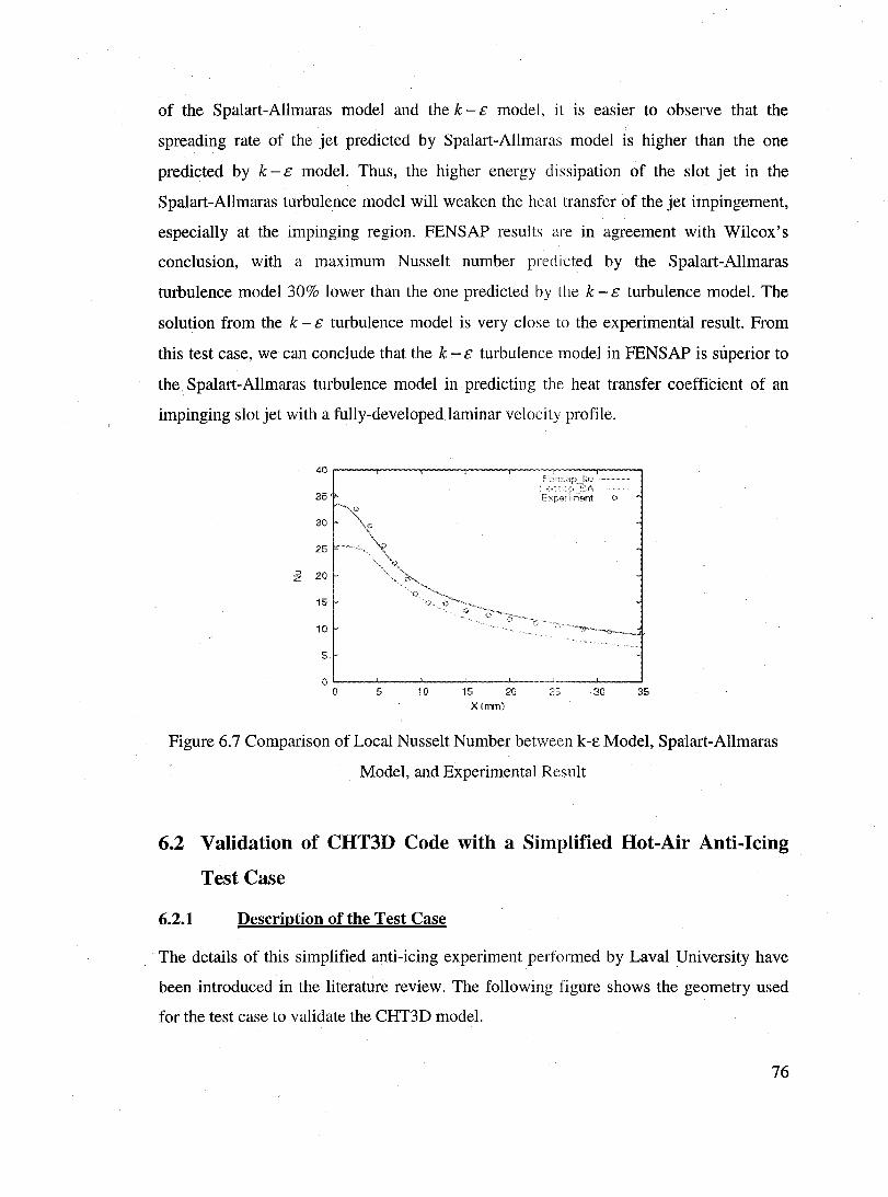
of the Spalart-Allmaras model and the k - ê model, it is easier to observe that the
spreading rate of the jet predicted by Spalart-Allmaras model is higher than the one
predicted by k - ê model. Thus, the higher energy dissipation of the slot jet in the
Spalart-Allmaras turbulence model will weaken the heat transfer of the jet impingement,
especially at the impinging region. FENSAP results are in agreement with Wilcox's
conclusion, with a maximum Nusselt number predicted by the Spalart-Allmaras
turbulence model 30% lower than the one predicted by the k - ê turbulence model. The
solution from the k - ê turbulence model is very close to the experimental result. From
this test case, we can conclude that the k - ê turbulence model in FENSAP is superior to
the. Spalart-Allmaras turbulence model in predicting the heat transfer coefficient of an
impinging slot jet with a fully-developed laminar velocity profile.
40
35'
30
25
::J 20 z
15
10
5
0 0 5 10 15 20 25 30 35
X (ml11)
Figure 6.7 Comparison of Local Nusselt Number between k-E Model, Spalart-Allmaras
Model, and Experimental Result
6.2 Validation of CHT3D Code with a Simplified Hot-Air Anti-lcing
Test Case
6.2.1 Description of the Test Case
The details of this simplified anti-icing experiment performed by Laval University have
been introduced in the literature review. The following figure shows the geometry used
for the test case to validate the CHT3D model.
76
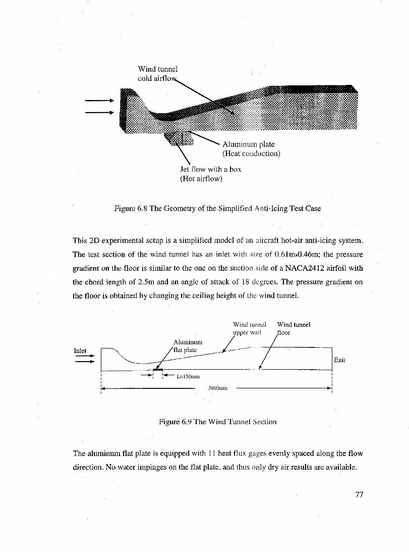
Wind tunnel cold
Aluminum plate (Heat conduction)
Jet flow with a box (Hot airflow)
Figure 6.8 The Geometry of the Simplified Anti-Icing Test Case
This 2D experimental setup is a simplified model of an aireraft hot-air anti-icing system.
The test section of the wind tunnel has an inlet with size of O.61mx0.46m; the pressure
gradient on the floor is similar to the one on the suction side of a NACA2412 airfoil with
the ehord length of 2.5m and an angle of attack of 18 degrees. The pressure gradient on
the floor is obtained by ehanging the eeiling height of the wind tunnel.
Inlet --, , ,. -' , :-- L=150mm
3660mm
Wind tunnel Wind tunnel oor
, , ----------_., ,
Figure 6.9 The Wind Tunnel Section
Exit
The aluminum flat plate is equipped with Il heat flux gages evenly spaced along the flow
direction. No water impinges on the flat plate, and thus only dry air results are available.
77

impinging jet flow
Figure 6.10 The Aluminum Flat Plate Section
The following figure shows the detailed geometry of the impinging jet flow enc10sed
within an aluminum box. Contrary to most aircraft anti-icing systems, the air at the jet
nozzle is not choked and is essentially a fully-developed laminar flow.
Impinging wall
with he t
Adiabatic wall
~
Jet Inlet
1 \1 \ Exit Adiabatic wall Exit
Figure 6.11 The Impinging Jet Section
6.2.2 Initial Wind Tunnel Airflow Simulation
Mesh:
78
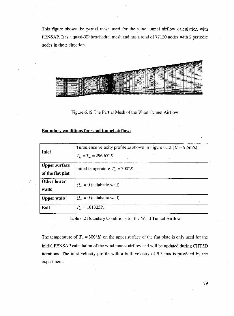
This figure shows the partial mesh used for the wind tunnel airflow calculation with
FENSAP. It is a quasi -3D hexahedral mesh and has a total of 77120 nodes with 2 periodic
nodes in the z direction.
Figure 6.12 The Partial Mesh of the Wind Tunnel Airflow
Boundary conditions for wind tunnel airflow:
Turbulence velocity profile as shown in Figure 6.13 (U = 9.5m1s) Inlet
T. =T =29665°K ln 00 •
Upper surface Initial temperature Tw = 300° K
of the flat plat
Other lower Qw = 0 (adiabatic wall)
walls
Upperwalls Qw = 0 (adiabatic wall)
Exit P= = 10 1325P a
Table 6.2 Boundary Conditions for the Wind Tunnel Airflow
The temperature of Tw = 300° K on the upper surface of the flat plate is only used for the
initial FENSAP calculation of the wind tunnel airflow and will be updated during CHT3D
iterations. The inlet velo city profile with a bulk velocity of 9.5 mis is provided by the
experiment.
79
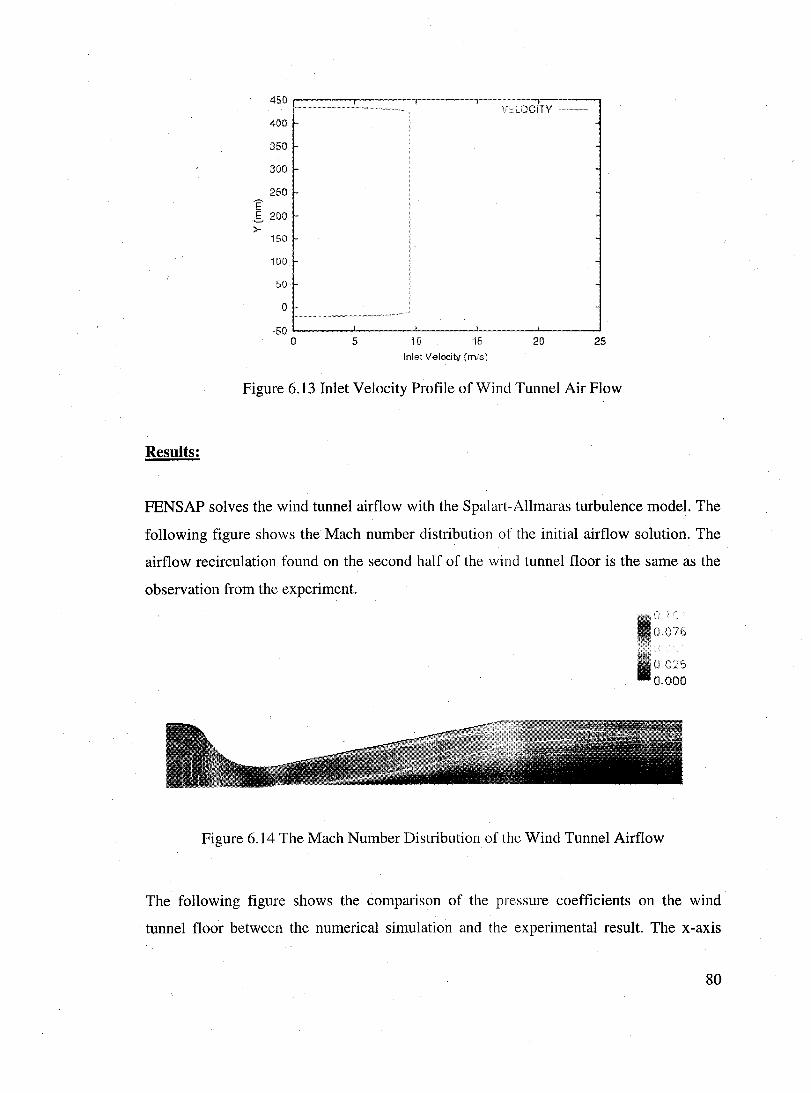
450 ,------,.----,..----.,.-------,.---....., V[LOGITY
400
350
300
250 Ê É, 200 >-
150
100
50
o
-50~----~-----~------~---~-----~ o 5 10 15 20 25
Inlet Velocity (mis)
Figure 6.13 Inlet Velocity Profile of Wind Tunnel Air Flow
Results:
FENSAP solves the wind tunnel airflow with the Spalart-Allmaras turbulence model. The
following figure shows the Mach number distribution of the initial airflow solution. The
airflow recirculation found on the second half of the wind tunnel floor is the same as the
observation from the experiment.
l,' 0 r"'>h .~Jk J
0.000
Figure 6.14 The Mach Number Distribution of the Wind Tunnel Airflow
The following figure shows the comparison of the pressure coefficients on the wind
tunnel floor between the numerical simulation and the experimental result. The x-axis
80
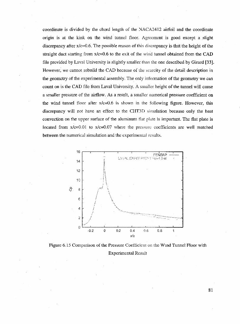
coordinate is divided by the chord length of the NACA2412 airfoil and the coordinate
origin is at the kink on the wind tunnel fIoor. Agreement is good except a slight
discrepancy after x/c=O.6. The possible reason of this discrepancy is that the height of the
straight duct starting from x/c=O.6 to the exit of the wind tunnel obtained from the CAD
file provided by Laval University is slightly smaller than the one described by Girard [33].
However, we cannot rebuild the CAD because of the scarcity of the detail description in
the geometry of the experimental assembly. The only information of the geometry we can
count on is the CAD file from Laval University. A smaller height of the tunnel will cause
a smaller pressure of the airflow. As a result, a smaller numerical pressure coeffkient on
the wind tunnel floor after x/c=O.6 is shown in the following figure. However, this
discrepancy will not have an effect to the CHT3D simulation because only the heat
convection on the upper surface of the aluminum fiat plate is important. The fiat plate is
located from x/c=O.Ol to x/c=O.07 where the pressure coefficients are weIl matched
between the numerical simulation and the experimental results.
16
14
12 ~
10
a.. 8 '-,) *
6
4 *
2
0 -0.2 0 0.2 OA 0.6 0.8 1
xie
Figure 6.15 Comparison of the Pressure Coefficienl on the Wind Tunnel Floor with
Experimental Result
81
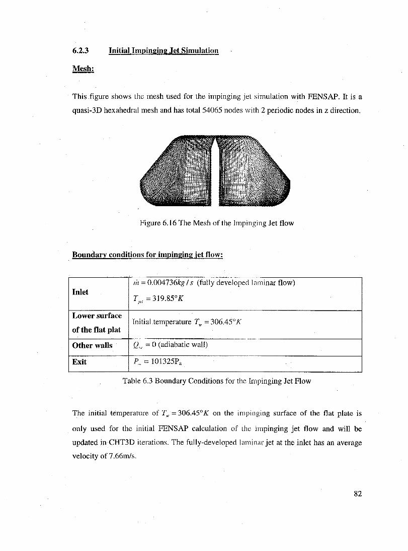
6.2.3 Initial Impinging Jet Simulation
Mesh:
This figure shows the mesh used for the impinging jet simulation with FENSAP. It is a
quasi-3D hexahedral mesh and has total 54065 nodes with 2 periodic nodes in z direction.
Figure 6.16 The Mesh of the Impinging Jet flow
Boundarv conditions for impinging jet flow:
n1 = 0.004736kg / s (fully developed laminar flow) Inlet
T jet = 319.85°K
Lower surface Initial temperature Tw = 306.45° K
of the flat plat
Other walls Qw = 0 (adiabatic wall)
Exit P= = 101325Pa
Table 6.3 Boundary Conditions for the Impinging Jet Flow
The initial tèrnperature of Tw = 306.45° K on the impinging surface of the fiat plate is
only used for the initial FENSAP calculation of the i mpinging jet flow and will be
updated in CHT3D iterations. The fully-developed laminar jet at the inlet has an average
velocity of 7.66m1s.
82
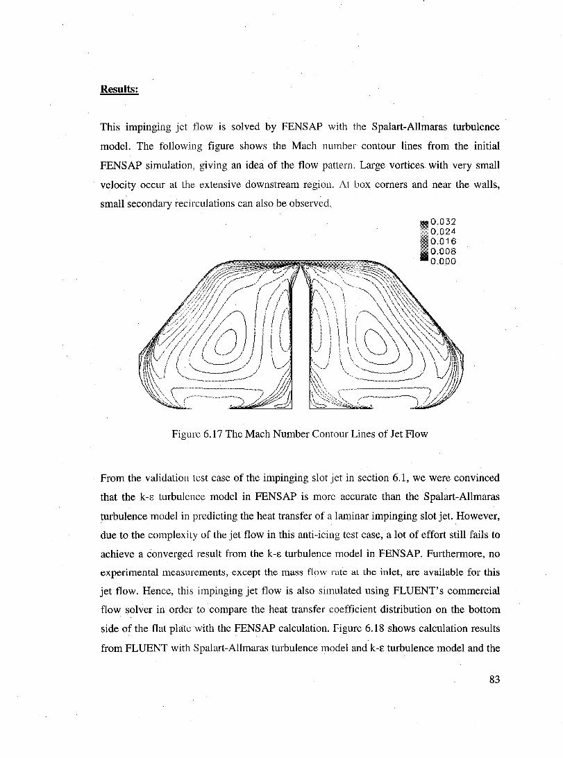
Results:
This impinging jet flow is solved by FENSAP with the Spalart-Allmaras turbulence
model. The following figure shows the Mach number contour Hnes from the initial
FENSAP simulation, giving an idea of the flow pattern. Large vortices with very small
velocity occur at the extensive downstream region. At box corners and near the walls, , .
small secondary recirculations can also be observed.
0,032 0,024
l, '0.016 1 0.008
0.000
Figure 6.17 The Mach Number Contour Lines of Jet Flow
From the validation test case of the impinging slot jet in section 6.1, we were convinced
that the k-E turbulence model in FENSAP is more accurate than the Spalart-Allmaras
~urbulence model in predicting the heat transfer of a laminar impinging slot jet. Rowever,
due to the complexity of the jet flow in this anti-icing test case, a lot of effort still fails to
achieve a converged result from the k-E turbulence model in FENSAP. Furthermore, no
experimental measurements, except the mass flow rate at the inlet, are available for this
jet flow. Rence, this impinging jet flow is also simulated using FLUENT's commercial
flow solver in order to compare the heat transfer coefficient distribution on the bottom
side of the flat plate with the FENSAP calculation. Figure 6.18 shows calculation results
from FLUENT with Spalart-Allmaras turbulence model and k-ê turbulence model and the
83

calculation result from FENSAP with Spalart-Allmaras turbulence model. The heat
transfer coefficients predicted by both flow solvers are very close in most are as , except
that the maximum value predicted by FENSAP is 30% higher than that predicted by
FLUENT at the impinging region.
250 - - - - - - Fluent S-A - --- -- Fluent K-E --- Fensap
200
o 0.02 0.04 0.06 0.08 x(m)
Figure 6.18 Comparison of Reat Transfer Coefficient Distribution on Impinging Surfaee
Without experimental results, it is hard to tell which the best result is. The difference
between the two flow solvers results may be caused by the fact that FENSAP's mesh was 1
used for the FLUENT calculation and may not be adapted to FLUENT' s needs. In
addition, it is possible that the artificial viscosity scheme is too dissipative in FLUENT.
Globally, it seems that FENSAP predicts higher heat flux than FLUENT. That means
FLUENT cannot give a better result as what we expect and is even worse than the result
from the FENSAP calculation with the Spalart-Allmaras turbulence model.
6.2.4 CHT3D Numerical Simulation
In the Laval University anti-ieing experiment, the material properties of the aluminum flat
plate are not specified. Renee, the following thermal properties of pure aluminum are
chosen for the flat plate:
Density: 2702 kg/m3
Thermal conductivity: 200 W/m.K
Specifie heat: Cp=900J/kg.K
84
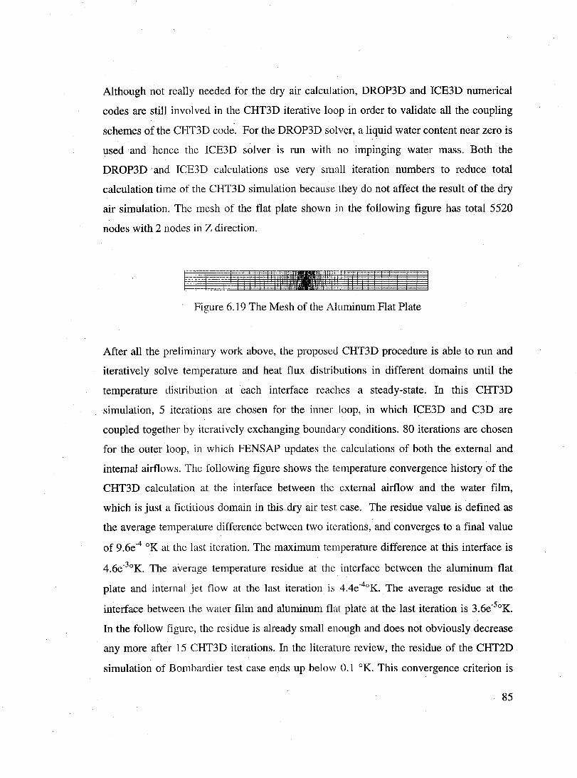
Although not really needed for the dry air calculation, DROP 3D and ICE3D numerical
codes are still involved in the CHT3D iterative loop in order to validate aIl the coupling
schemes of the CHT3D code. For the DROP3D solver, a liquid water content near zero is
usedand hence the ICE3D solver is run with no impinging water mass. Both the
DROP3D 'and ICE3D calculations use very small iteration numbers to reduce total
calculation time of the CHT3D simulation because they do not affect the result of the dry
air simulation. The mesh of the flat plate shown in the following figure has total 5520
nodes with 2 nodes in Z direction.
Figure 6.19 The Mesh of the Aluminum Flat Plate
After aIl the preliminary work above, the proposed CHT3D procedure is able to run and
iteratively solve temperature and heat flux distributions in different domains until the
temperature distribution at each interface reaches a steady-state. In this CHT3D
simulation, 5 iterations are chosen for the inner Ioop, in which ICE3D and C3D are
coupled together by iteratively exchanging boundary conditions. 80 iterations are chosen
for the outer Ioop, in which FENSAP updates the calculations of both the external and
internaI airflows. The following figure shows the temperature convergence history of the
CHT3D calculation at the interface between the external airflow and the water film,
which is just a fictitious domain in this dry air test case. The residue value is defined as
the average temperature difference between two iterations, and converges to a final value
of 9.6e-4 OK at the last iteration. The maximum temperature difference at this interface is
4.6e-30K. The average temperature residue at the interface between the aluminum flat
plate and interna] jet flow at the last iteration is 4.4e-40K. The average residue at the
interface between the water film and aluminum flat plate at the last iteration is 3.6e-s0K.
In the follow figure, the residue is already small enough and does not obviously decrease
any more after 15 CHT3D iterations. In the literature review, the residue of the CHT2D
simulation of Bombardier test case ends up below 0.1 oK. This convergence criterion is
85
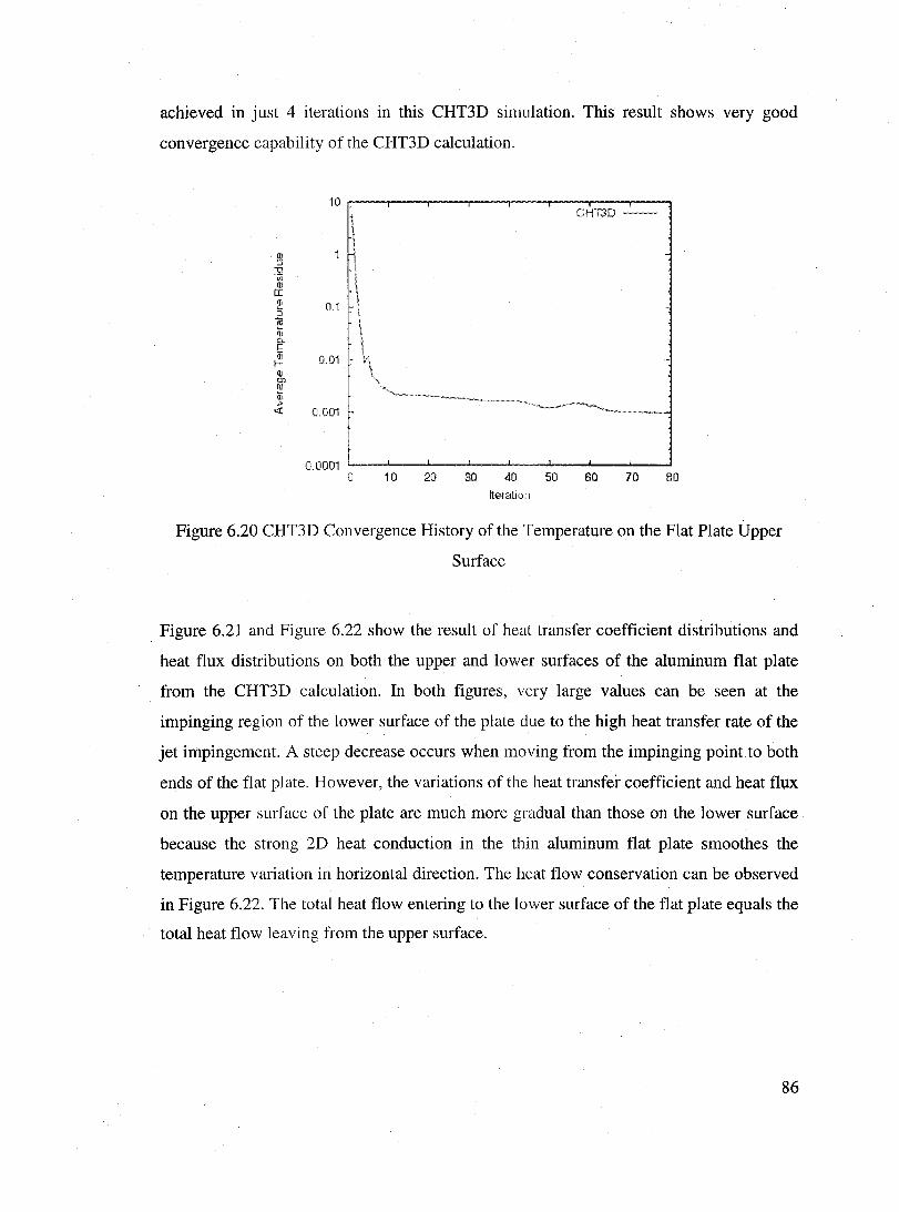
achieved in just 4 iterations in this CHT3D simulation. This result shows very good
convergence capability of the CHT3D calculation.
10 r---.---,,---r---.----.---.---,---~ GHTSD --
0.0001 '--_-'--_-1-_--'-_-"' __ '--_"'--_ .... '_---'
o 10 20 30 40
Iteration
50 60 70 80
Figure 6.20 CHT3D Convergence History of the Temperature on the Flat Plate Upper
Surface
. Figure 6.21 and Figure 6.22 show the result of heat transfer coefficient distributions and
heat flux distributions on both the upper and lower surfaces of the aluminum flat plate
from the CHT3D calculation. In both figures, very large values can be seenat the
impinging region of the lower surface of the plate due to the high heat transfer rate of the
jet impingement. A steep decrease occurs when moving from the impinging poinuo both
ends of the flat plate. However, the variations of the heat transfei- coefficient and heat flux
on the upper surface of the plate are much more graduaI than those on the lower surface
because the strong 2D heat conduction in the thin aluminum flat plate smoothes the
temperature variation in horizontal direction. The heat flow conservation can be observed
in Figure 6.22. The total heat flow entering to the \ower surface of the flat plate equals the
total heat flow leaving from the upper surface.
86
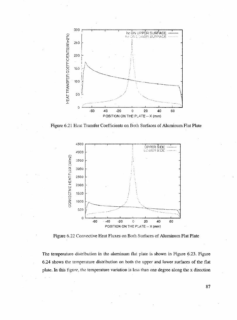
300 :.;;;-• C\I E: 250 . ~ fli r z 200 I,!! 0 u:: LL w 150 0 0 0: w LL 100 lf)
z ~ r
50 ~
o l w J:
-60 40 -20 0 20 40 60 POSITION ON THE PLATE -- X (mm)
Figure 6.21 Heat Transfer Coefficients on Both Surfaces of Aluminum Flat Plate
4500 UPPERSIDE ~ .. -
4000 2;iOE,
(,t E ~
35000 ~
x 3000 ::J .-J LL t-4.;
25000 w J: 2000 w ~ t- 1500 0 w > z 0
1000 0
500
0 -60 ;40 -20 0 20 40 60
POSITION ON THE PLATE -- X (mm)
Figure 6.22 Convective Heat Fluxes on Both Surfaces of Aluminum Flat Plate
The temperature distribution in the aluminum flat plate is shown in Figure 6.23. Figure
6.24 shows the temperature distribution on both the upper and lower surfaces of the. flat
plate. In this figure, the temperature variation is less than one degree along the x direction
87
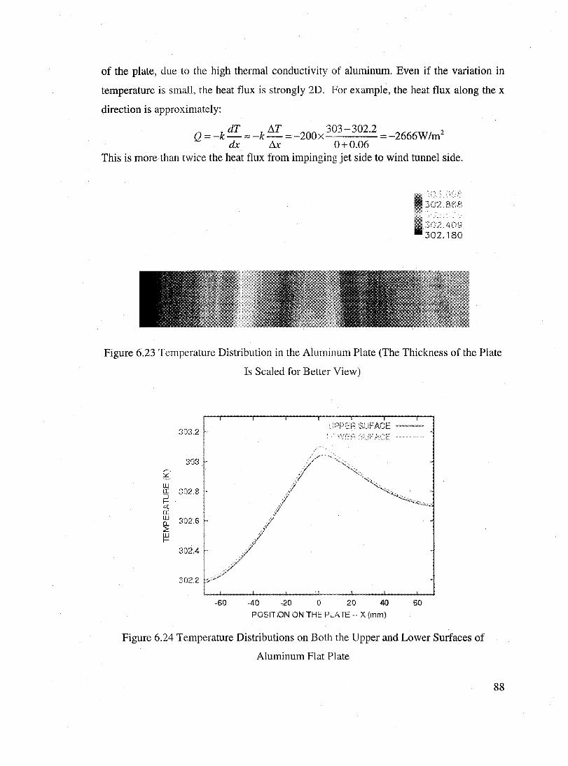
of the plate, due to the high thermal conductivity of aluminum. Even if the variation in
temperature is small, the heat flux is strongly 2D. For example, the heat flux along the x
direction is approximately:
Q =-k dT ~ -k I1T =-200x 303-302.2 =-2666W/m2
dx l1x 0+0.06 This is more th an twice the heat flux from impinging jet side to wind tunnel side.
Figure 6.23 Temperature Distribution in the Aluminum Plate (The Thickness of the Plate
Is Scaled for Better View)
303.2
::::03
w 0:: :J
302.8 t-.-( ct w 302.6 Il. ~ W 1-
302.4
302.2
-60 -40 -20 1) 20 40 60
POSITION ON THE PU\ TE -- X (mm)
Figure 6.24 Temperature Distributions on Bath the Upper and Lower Surfaces of
Aluminum Flat Plate
88
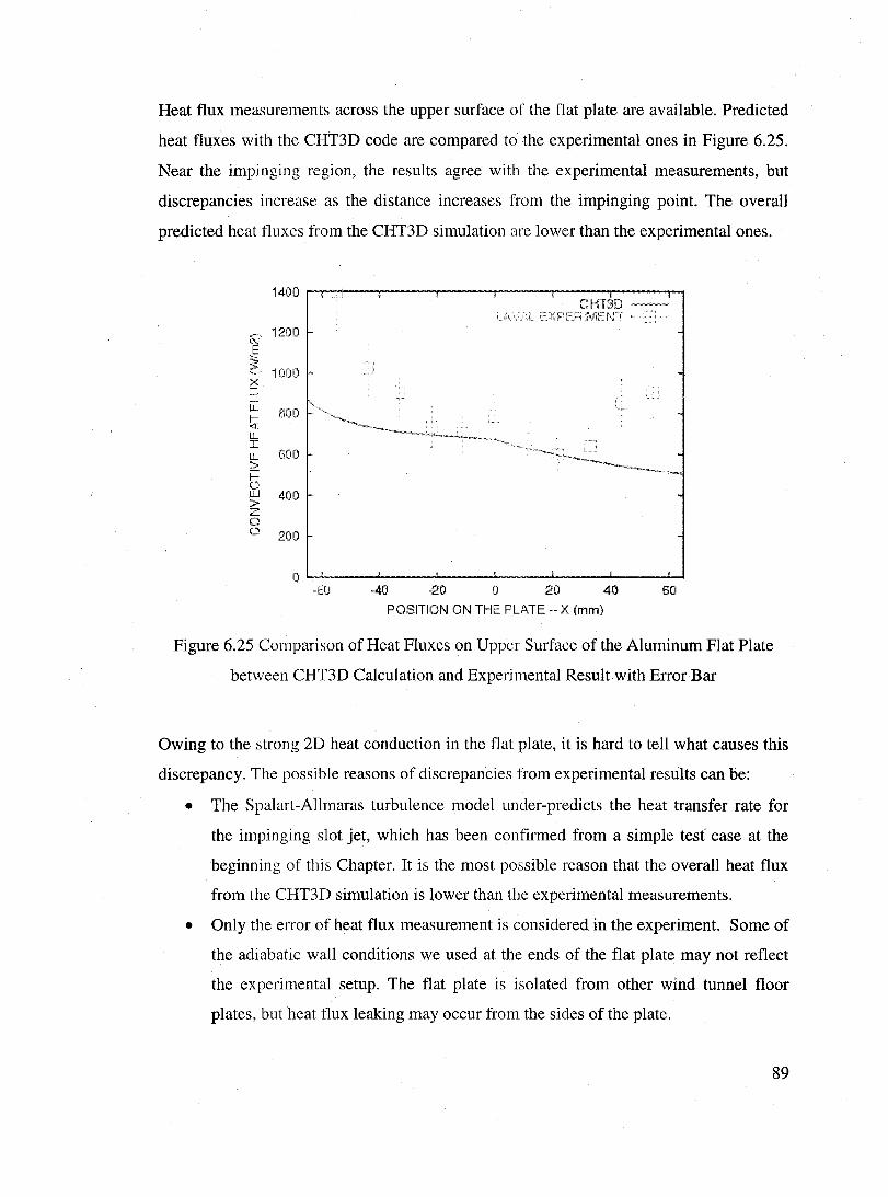
Heat flux measurements across the upper surface of the flat plate are av ail able. Predicted
heat fluxes with the CHT3D code are compared to the experimental ones in Figure 6.25.
Near the impinging region, the results agree with the experimental measurements, but
discrepancies increase as the distance increases from the impinging point. The overall
predicted heat fluxes from the CHT3D simulation are lower than the experimental ones.
1400 CHT3D -'-'-
. L lrI1EI\(T
N' 1200 E ~>, 1000 X =:l ...J LL
800 ~ W I W 600 2:
b ,w 400 > z 0 Cl 200
0 -60 -40 -20 0 20 40 60
POSITION ON THE PLATE -- X (mm)
Figure 6.25 Comparison of Heat Fluxes on Upper Surface of the Aluminum Flat Plate
between CHT3D Ca1culation and Experimental Result with Error Bar
Owing to the strong 2D heat conduction in the flat plate, it is hard to tell what causes this
discrepancy. The possible reasons of discrepancies from experimental results can be:
• The Spalart-Allmaras turbulence model under-predicts the heat transfer rate for
the impinging slot jet, which has been confirmed from a simple test case at the
beginning of this Chapter. It is the most possible reason that the overall heat flux
from the CHT3D simulation is lower than the experimental measurements.
• Only the error of heat flux measurement is considered in the experiment. Sorne of
the adiabatic wall conditions we used at the ends of the flat plate may not reflect
the ex periment al setup. The flat plate is isolated from other wind tunnel floor
plates, but heat flux leaking may occur from the sides of the plate.
89
• Heat conductivity of the flat plate is not specified in the experiment and it will
affect the heat flux results. The higher heat conductivity will transfer more heat
flux to the ends of the flat plate from the impinging region due to the strong heat
conduction in horizontal direction of the flat plate.
Nevertheless, the. overall CHT3D procedure does not seems to be responsible for the
discrepancy. Investigations are still needed before we can conc1ude the study and further
validation may be carried out by Bombardier on its proprietary geometries and data.
6.3 Conclusions
The CHT3D procedure has been validated against a 2D dry air anti-icing experimental
test case with partial success. It can successfully simulate and solve hot-air anti-icing
problems. The discrepancies between the numerical simulation and the experimental
measurement do not seem to be the responsibiliti' of the coupling procedure in the
numerical code but the turbulence model used to solve the jet flow or the experimental
setup. The numerical result of the impinging jet shows how an anti-icing system
simulation can rapidly grow in complexity, even in 2D. Further investigations and efforts
may be still needed to improve the results of the numerical simulation.
90

Conclusions and Future Work
Due to the great impact on flight safety by in-flight ice accretion, effective ice protection
measures have to be applied against in-flight ice buildup. To design efficient hot-air anti
icing systems is very important in order to reduce the penalties due to the bleeding air
from engines. CFD tools are continuously being developed to assist in anti-icing system
design and in certification of aircraft. In this thesis, a 3D conjugate heat transfer module
(CHT3D) has been developed to simulate hot-air anti-icing processes based on a loose
coupling procedure, which has great flexibility in solving complicated conjugate heat
transfer problerns. Different numerical methods for the general CHT and hot-air anti-icing
simulations have been discussed in the literature review. The CHT3D module uses the
currently available 3D CFD package FENSAP-ICE to iteratively solve the external cold
airflow, water filrnlice accretion, solid conduction, and internaI hot airflow based on
iteratively exchanging thermal boundary conditions at common interfaces of different
domains. The rnathernatical equations and numerical methods used for solving different
domains have been presented in chapter 3 and the CHT3D algorithm has been elaborated
in chapter 4. Robin boundary conditions are irnposed at most of the interfaces as a
relaxation scherne for CHT3D coupling and have been proved to be robust in eliminating
the numerical instability. Currently, aIl domains coupled by CHT3D must have matching
grids at their common interfaces, which can accurately exchange boundary conditions but
is difficult for industrial level simulations with complex geometries. A virtual grid
technique for boundary condition exchanges to non-matching grids has been introduced
and can be irnplernented into the current CHT3D code.
In chapter 5, CHT3D code has been tested to successfully simulate the full range of anti
icing cases. The verification test cases are simple but comprehensive enough to test the
full capabilities of the CHT3D code. The results of CHT3D simulations for these test
cases are in agreement with the physical observations.
In chapter 6, CHT3D has been validated against a simplified 2D hot-air anti-icing
experiment performed by Laval University. This experiment mimics a real hot-air anti-
91

icing system with flow around a wing, internaI impinging jet flow and solid conduction,
but without droplet impingement. This experiment is the most suitable we can find to
validate the CHT3D code. The simulation results are partially successful in comparison
with the experimental results of heat fluxes. It does not seem that the discrepancies are
related to the CHT3D procedure but most likely the shortcomings of the turbulence model
for impinging jets and to the errors in experimental setup.
To sum up, the CHT3D procedure developed in this thesis has been proven successful in
simulating the hot-air anti-icing processes. However, its applications are not only limited
in anti-icing simulation. It can also apply to any CHT problems with two air/fluid flows
separated by a solid with/without the water film on the external surface of the solid.
Sorne future work may involve the following:
• Further effort to solve the impinging jet in Laval test case with k-E turbulence
model.
• Add the capability into the current CHT3D code of exchanging boundary
conditions for non-matching grids.
• 2D and 3D experiments including water runback and evaporation effects would be
needed to further validate the CHT3D code.
92

Bibliography
[1] Kind RJ., Icing, frost and aircraft flight, Canadian Aeronauties and Spaee Journal,
Vol. 44, No. 2, pp. 110-118, June 1998.
[2] Render P.M., Jenkinson L.R, Investigation into Ice Detection Parameters for
Turboprop Aircraft, Journal of Aireraft, 33(1), pp. 125-130, 1996.
[3] Thomas S. K., Cassoni R P., and MacArthur C. D., Aircraft Anti-lcing and De
Icing Techniques and Modeling, Journal of Aireraft, Vol.33, No. 5, pp. 841-854,
September-October 1996.
[4] Al-Khali] K.M., Horvath c., Miller D.R, and Write W.B., Validation of NASA
Thermal !ce Protection Computer Codes. III-The Validatiol) of ANTICE, AlAA
Paper 97-0051, Jan. 1997
[5] Yeoman K., Efficiency of a Bleed Air Powered Inlet Icing Protective' System,
AlAA Paper 94-0717, 32nd Aerospace Sciences Meeting & Exhibit, Reno, NV, Jan.
1994.
[6] Dornheim A. M., Electric Cabin, Aviation Week & Space Teehnology, Vo1.162,
Iss.l3, pp. 47, New York, Mar.28, 2005
[7] Habashi W.G., Nadarajah S., Aube M., Pueyo A., Dow J.P., Effective Use of CFD
for In-flight Icing Certification, June, 2004
[8] Wright, W. B., User Manual for the NASA Glenn Ice Accretion Code LEWICE
Version 2.2.2, NASA/CR-2002-211793, NASA, Aug. 2002
[9] Brahimi M. T., Tran P., and Paraschivoiu I., Numerical Simulation and
Thermodynamic Analysis of Ice Accretion on Aircraft Wings, Final Report, C.D.T.
Projeet CJ59, prepared for Bombardier Inc./Canadair, Montreal, Canada, May 1994
[10] FENSAP-ICE User's Guide, Version 2005 RI Beta2, Newmerical Technologies Int.
[11] Chmielniak T., Wroblewski W., Nowak G., Wecel D., Coupled Analysis of Cooled
Gas Turbine Blades, ASME paper GT2003-38657, 2003
[12] Marini R, A Finite Element Conjugate Heat Transfer Method, Master Thesis,
Concordia University, Canada, 2002
93

[13] Giles M. B., Stability Analysis of Numerical Interface Conditions in Fluid-Structure
Thermal Analysis, Int. J. for Numerical Methods in Fluids, Vol. 25, pp. 421-436,
John Wiley & Sons, Ltd. 1997
[14] Croce G., and Habashi W. G., Thermal Analysis of Wing and Nacelle Anti-Icing
Devices, Computational Analysis of Convection Heat Transfer, Chapter 10, pp.
409-432, Wessex Institute of Technology Press, 2000
[15] Croce G., Habashi W. G., Guevremont G., and Tezok F., 3D Thermal Analysis of
an Anti-Icing Deviee Using FENSAP-ICE, AIAA Paper 98-0193,1998
[16] Croce G., Beaugendre H., and Habashi W. G., CHT 3D: FENSAP-ICE Conjugate
Heat Transfer Computations with Droplet Impingement and Runback Effects, AlAA
Paper 2002-0386, 40th Aerospace Sciences Meeting & Exhibit, Reno, NV, Jan.
2002
[17] Croce G., A Conjugate Heat Transfer Procedure for Gas Turbine Blades, Heat
Transfer in Gas Turbine Systems, Annals of N.Y. Academy of Sciences, pp. 273-
280,2001
[18] Funaro D., Quarteroni A., and Zanolli P., An Iterative Procedure with Interface
Relaxation for Domain Decomposition Methods, SIAM J. Numer. Analysis, Vol. 25
n.6, pp. 1213-1236,1988.
[19] Imlay S. T., Soetrisno M., and Roberts D. W., Coupled Flow and Heat Transfer
Analysis using Structured-Unstructured Grids, AlAA Paper 96-0622, 34th
Aerospace Sciences Meeting & Exhibit, Reno, NV, Jan. 1996
[20] Montenay A., Pate, and Duboue J. M., Conjugate Heat Transfer Analysis of an
Engine InternaI Cavity, ASME Paper 2000-GT-282, May 2000
[21] Kassab A., Divo E., Heidmann J., Steinthorsson E., and Rodriguez F., BEMIFVM
Conjugate Heat Transfer Analysis of a Three-Dimensional Film Cooled Turbine
Blade, International Journal of Numerical Methodsfor Heat & Fluid Flow, Vol. 13
No.5, 2003, pp. 581-610
[22] AI-Khalil K.M., Numerical Simulation of an Aircraft Anti-icing System
Incorporation a Rivulet Model for the Runback Water, PHD Thesis, The University
of Toledo
94
[23] Hess J.L., and Smith AM.O., Ca1culation of Potential Flow About Arbitrary Bodies,
Progress in Aeronautical Sciences, 8:1-138, (D. Kuchemann editor), Elmsford,
New York, Pergmon Press, 1967
[24] Messinger B.L., Equilibrium Temperature of an Unheated king Surface as a
Function of Air Speed, Journal of the Aeronautical Sciences, Vol. 20, No.1, pp. 29-
42, 1953
[25] Wright W. B., An Evaluation of Jet Impingement Heat Transfer Correlations for
Piccolo Tube Application, NASA/CR-2004-212917, NASA Glenn Research Center,
April 2004
[26] Pueyo A, Chocron D., Mokhtarian F., Kafyeke F., CHT2D: A 2D Hot Air Anti
Icing Analysis Tool, 50th Annual General Meeting (AGM) and Conference,
Canadian Aeronautics and Space Institute, 2003
[27] Tran P., Brahimi M. T., Paraschivoiu L, Pueyo A. and Tezok F., Ice Accretion on
Aircraft Wings with Thermodynamic Effects, Journal of Aircraft, Volume 32, n. 2,
1994
[28] Pueyo A, Chocron D. and Kafyeke F., Improvements to the Ice Accretion Code
CANICE, CAS! 8th Aerodynamics Symposium, Toronto May, 2001
[29] Mavriplis D. J., and Venkatakrishnan v., Agglomeration Multigrid for Two
Dimensional Viscous Flows, Computers and Fluids, 24(5):553-570, May 1995
[30] Mavriplis D. J., and Venkatakrishnan V., A Unified Multigrid Solver for the
Navier-Stokes Equations on Mixed Element Meshes, AlAA Paper 95-1666, June
1995
[31] Morency F., Tezok F., Paraschivoiu L, Anti-Icing System Simulation Using
CANICE, Journal of Airerait, Vol. 36, No. 6, November-December, 1999
[32] Morency E, Tezok E, Paraschivoiu L, Heat and Mass Transfer in the Case of Anti
Icing System Simulation, Journal of Aircraft, Vol. 37, No. 2, March-April, 2000
[33] Girard E, Mesure du Flux de Chaleur d'un Modèle Simplifié d'un Système
Antigivre d'Aile d'Avion, thèse de maîtrise, l'Université Laval, 2004
[34] Baruzzi G.S., Habashi W.G., Guevremont J.G., Hafez M.M., A Second Order Finite
Element Method for the Solution of the Transonic Euler and Navier-Stokes
95

Equations, International Journal for Numerical Methods in Fluids, Vol.20, 671-693,
1995
[35] Spalart Ph.R., Trends in turbulence Treatments, A1AA Paper 2000-2306, 2000
[36] Beaugendre H., Morency F., and Habashi W.G., FENS AP-ICE: Roughness Effects
on Ice Shape Prediction, A1AA Paper 2003-1222,41 st Aerospace Sciences Meeting
& Exhibit, Reno, Nevada, Jan. 2003
[37] Gresho P. M., Lee R. L., Sani R. L., Maslanik M. K., Eaton B. E., The Consistent
Galerkin FEM For Computing Derived Boundary Quantities in Thermal and/or
Fluids Problems, International Journal for Numerieal Methods in Fluids, Vol.7, pp.
371-394, 1987
[38] Bourgault Y., Habashi W.G., Dompierre J., and Baruzzi G., A Finite Element
Method Study of Eulerian Droplets Impingement Models, Int. J. Numer. Meth.
Fluids, 1999
[39] Honsek, R., Development of a Three-Dimensional Eulerian Model of Droplet-Wall
Interaction Mechanisms, Master Thesis, Mc Gill University, Montreal, QC, 2005
[40] Bourgault Y., Beaugendre H., and Habashi W.G., Development of a Shallow-Water
Icing Model in FENSAP-ICE, Journal of Aireraft, Vol.37, No.4, July-August 2000
[41] Beaugendre H., Morency F., and Habashi W.G., FENSAP-ICE's Three
Dimensional In-Flight !ce Accretion Module: ICE3D, Journal of Aireraft, Vol.40,
No.3, May-June, 2003
[42] Beaugendre H., A PDE-Based 3D Approach to In-Flight Ice Accretion, PHD Thesis,
McGill University, Montreal, QC, 2003
[43] Hirsch Ch., "Numerical Computation of InternaI and External Flows", Volume 2:
"Computational Methods for Inviscid and Viseous Flows", John Wiley & sons,
1988
[44] Toro E.F., "Riemann Soivers and Numerical Methods for Fluid Dynamics, A
Practical Introduction", Springer, 1999
[45] Roe P.L., "Approximate Riemann Solvers, Parameter Vectors, and Difference
Schemes", Journal ofComputational Physics, Vol.43, pp357-372, 1981
[46] Lepage c., and H,abashi W.G., Conservative Interpolation of Aerodynamic Loads
for Aeroelastic Computations, AlAA Paper 2000-1449,2000
96
[47] Lepage c., A Tight Fluid-Structure Coupling for Aeroelastic Computations in the
Time Domain, PHD Thesis, Concordia University, Montreal, Quebec, Feb. 2004
[48] Sparrow E. M. and Wong T. c., Impingement Transfer Coefficients Due to Initially
LaminaI' Slot Jets, Int. J. Heat Mass Transfer, Vol. 18, pp. 597-605, Pergamon
Press 1975
[49] Martin H., Heat and Mass Transfer between Impinging Gas Jets and Solid Surfaces,
in J. P. Hartnett and T. F. Irvine, Jr., Eds., Advances in Heat Transfer, Vol. 13,
Academie Press, New York, 1977
[50] Wilcox D., Turbulence Modeling for CFD, 20d Edition, DCW Industries, 2004
97


