North Carolina Math 4
300
Program Overview North Carolina Math 4
Transcript of North Carolina Math 4

Program Overview
North Carolina Math 4

1 2 3 4 5 6 7 8 9 10
ISBN 978-0-8251-9073-5
Copyright © 2020
J. Weston Walch, Publisher
Portland, ME 04103
www.walch.com
Printed in the United States of America
© Common Core State Standards. Copyright 2010. National Governor’s Association Center for Best Practices and
Council of Chief State School Officers. All rights reserved.
The classroom teacher may reproduce these materials for classroom use only.The reproduction of any part for an entire school or school system is strictly prohibited.
No part of this publication may be transmitted, stored, or recorded in any formwithout written permission from the publisher.
This program was developed and reviewed by experienced math educators who have both academic and professional backgrounds in mathematics. This ensures: freedom from mathematical errors, grade level
appropriateness, freedom from bias, and freedom from unnecessary language complexity.
Developers and reviewers include:
Jasmine Owens
Joanne N. Whitley
Shelly Northrop Sommer
Joyce Hale
Jake Todd
Shawn Pilling
Ruth Estabrook
Pam Loveridge
James Gunnin
Robert Leichner
Joseph Nicholson
Kristine Chiu
Chris Moore
Kaitlyn Hollister
Samantha Carter
Dawn McNair
Jack Loynd
Terri Germain-Williams
Laura McPartland
David Rawson
Lenore Horner
Nancy Pierce
Dale Blanchard
Pamela Rawson
Valerie Ackley
Lynze Greathouse
Jane Mando
Timothy Trowbridge
Alan Hull
Angela Heath
Linda Kardamis
Cameron Larkins
Frederick Becker
Kimberly Brady
Corey Donlan
Pablo Baques
Mike May, S.J.
Whit Ford
Heather Morton
Deborah Benton
Erin Brack
Kim Brady

North Carolina Math 4 Teacher Resource
© Walch Educationiii
Table of Contents for Instructional Units . . . . . . . . . . . . . . . . . . . . . . . . . . . . . . . . . . . . . . . . . . . . . . . . vIntroduction to the Program . . . . . . . . . . . . . . . . . . . . . . . . . . . . . . . . . . . . . . . . . . . . . . . . . . . . . . . . . . . 1Correspondence to Standards for Mathematical Practice . . . . . . . . . . . . . . . . . . . . . . . . . . . . . . . . . . . 4Unit Structure . . . . . . . . . . . . . . . . . . . . . . . . . . . . . . . . . . . . . . . . . . . . . . . . . . . . . . . . . . . . . . . . . . . . . . . . 5Standards Correlations . . . . . . . . . . . . . . . . . . . . . . . . . . . . . . . . . . . . . . . . . . . . . . . . . . . . . . . . . . . . . . . . 9Conceptual Activities . . . . . . . . . . . . . . . . . . . . . . . . . . . . . . . . . . . . . . . . . . . . . . . . . . . . . . . . . . . . . . . . . 15Digital Enhancements Guide . . . . . . . . . . . . . . . . . . . . . . . . . . . . . . . . . . . . . . . . . . . . . . . . . . . . . . . . . . 20Standards for Mathematical Practice Implementation Guide . . . . . . . . . . . . . . . . . . . . . . . . . . . . . . 22Instructional Strategies . . . . . . . . . . . . . . . . . . . . . . . . . . . . . . . . . . . . . . . . . . . . . . . . . . . . . . . . . . . . . . . 25Formulas . . . . . . . . . . . . . . . . . . . . . . . . . . . . . . . . . . . . . . . . . . . . . . . . . . . . . . . . . . . . . . . . . . . . . . . . . . F-1Glossary . . . . . . . . . . . . . . . . . . . . . . . . . . . . . . . . . . . . . . . . . . . . . . . . . . . . . . . . . . . . . . . . . . . . . . . . . . . G-1
iii
Contents of Program OverviewPROGRAM OVERVIEW


© Walch Educationv
North Carolina Math 4 Teacher Resource
Table of Contents for Instructional UnitsPROGRAM OVERVIEW
v
Unit 1: Building Mathematical Community with Parent Functions and Key FeaturesUnit 1 Resources . . . . . . . . . . . . . . . . . . . . . . . . . . . . . . . . . . . . . . . . . . . . . . . . . . . . . . . . . . . . . . . . . . . . U1-1
Lesson 1.1: Reading and Identifying Key Features of Real-World Situation Graphs (NC.M3.F–IF.4★) . . . . . . . . . . . . . . . . . . . . . . . . . . . . . . . . . . . . . . . . U1-5
Lesson 1.2: Transformations of Parent Graphs (NC.M3.F–BF.3) . . . . . . . . . . . . . . . . . . . . . . . . U1-54Lesson 1.3: Recognizing Odd and Even Functions (NC.M3.F–BF.3) . . . . . . . . . . . . . . . . . . . . . . U1-92
Answer Key . . . . . . . . . . . . . . . . . . . . . . . . . . . . . . . . . . . . . . . . . . . . . . . . . . . . . . . . . . . . . . . . . . . . . . . U1-111
Mid-Unit Assessment and Answer Key . . . . . . . . . . . . . . . . . . . . . . . . . . . . . . . . . . . . . . . . . . . . . . . MA-1
End-of-Unit Assessment and Answer Key . . . . . . . . . . . . . . . . . . . . . . . . . . . . . . . . . . . . . . . . . . . . . . EA-1
Unit 2: Piecewise Functions, Composition of Functions, and RegressionUnit 2 Resources . . . . . . . . . . . . . . . . . . . . . . . . . . . . . . . . . . . . . . . . . . . . . . . . . . . . . . . . . . . . . . . . . . . . U2-1
Lesson 2.1: Piecewise, Step, and Absolute Value Functions (NC.M4.AF.4.1, NC.M4.AF.4.2) . . . . U2-5Lesson 2.2: Composition of Functions (NC.M4.AF.1.1) . . . . . . . . . . . . . . . . . . . . . . . . . . . . . . . . U2-33Lesson 2.3: Evaluating Composite Functions in Various Forms (NC.M4.AF.1.2) . . . . . . . . . . . U2-56Lesson 2.4: Linear, Exponential, and Quadratic Regression (NC.M4.AF.5.1) . . . . . . . . . . . . . . U2-81Lesson 2.5: Analyzing Residual Plots (NC.M4.AF.5.2) . . . . . . . . . . . . . . . . . . . . . . . . . . . . . . . . U2-112
Answer Key . . . . . . . . . . . . . . . . . . . . . . . . . . . . . . . . . . . . . . . . . . . . . . . . . . . . . . . . . . . . . . . . . . . . . . . U2-155
Mid-Unit Assessment and Answer Key . . . . . . . . . . . . . . . . . . . . . . . . . . . . . . . . . . . . . . . . . . . . . . . MA-1
End-of-Unit Assessment and Answer Key . . . . . . . . . . . . . . . . . . . . . . . . . . . . . . . . . . . . . . . . . . . . . . EA-1

vi© Walch EducationNorth Carolina Math 4 Teacher Resource
PROGRAM OVERVIEWTable of Contents for Instructional Units
Unit 3: Logarithmic FunctionsUnit 3 Resources . . . . . . . . . . . . . . . . . . . . . . . . . . . . . . . . . . . . . . . . . . . . . . . . . . . . . . . . . . . . . . . . . . . . U3-1
Lesson 3.1: Inverses of Exponential and Logarithmic Functions (NC.M4.AF.3.1) . . . . . . . . . . . U3-3Lesson 3.2: Common Logarithms (NC.M4.AF.3.1, NC.M4.AF.3.2) . . . . . . . . . . . . . . . . . . . . . . U3-26Lesson 3.3: Natural Logarithms (NC.M4.AF.3.1, NC.M4.AF.3.2) . . . . . . . . . . . . . . . . . . . . . . . . U3-48Lesson 3.4: Interpreting Logarithmic Models
(NC.M4.AF.3.1, NC.M4.AF.3.2, NC.M4.AF.3.3) . . . . . . . . . . . . . . . . . . . . . . . . . . . . U3-81Lesson 3.5: Logarithmic Regression (NC.M4.AF.5.1) . . . . . . . . . . . . . . . . . . . . . . . . . . . . . . . . . U3-111
Answer Key . . . . . . . . . . . . . . . . . . . . . . . . . . . . . . . . . . . . . . . . . . . . . . . . . . . . . . . . . . . . . . . . . . . . . . . U3-147
Mid-Unit Assessment and Answer Key . . . . . . . . . . . . . . . . . . . . . . . . . . . . . . . . . . . . . . . . . . . . . . . MA-1
End-of-Unit Assessment and Answer Key . . . . . . . . . . . . . . . . . . . . . . . . . . . . . . . . . . . . . . . . . . . . . . EA-1
vi
Unit 4: TrigonometryUnit 4 Resources . . . . . . . . . . . . . . . . . . . . . . . . . . . . . . . . . . . . . . . . . . . . . . . . . . . . . . . . . . . . . . . . . . . . U4-1
Lesson 4.1: Proving the Fundamental Pythagorean Identity (NC.M4.AF.2.1) . . . . . . . . . . . . . . . U4-5Lesson 4.2: Proving the Law of Sines (NC.M4.AF.2.2) . . . . . . . . . . . . . . . . . . . . . . . . . . . . . . . . . U4-28Lesson 4.3: Proving the Law of Cosines (NC.M4.AF.2.2) . . . . . . . . . . . . . . . . . . . . . . . . . . . . . . . U4-65Lesson 4.4: Applying the Laws of Sines and Cosines (NC.M4.AF.2.2) . . . . . . . . . . . . . . . . . . . . U4-91Lesson 4.5: Key Features of Trigonometric Functions (NC.M4.AF.2.3) . . . . . . . . . . . . . . . . . . U4-123Lesson 4.6: Sinusoidal Regression (NC.M4.AF.5.1) . . . . . . . . . . . . . . . . . . . . . . . . . . . . . . . . . . . U4-162
Answer Key . . . . . . . . . . . . . . . . . . . . . . . . . . . . . . . . . . . . . . . . . . . . . . . . . . . . . . . . . . . . . . . . . . . . . . . U4-201
Mid-Unit Assessment and Answer Key . . . . . . . . . . . . . . . . . . . . . . . . . . . . . . . . . . . . . . . . . . . . . . . MA-1
End-of-Unit Assessment and Answer Key . . . . . . . . . . . . . . . . . . . . . . . . . . . . . . . . . . . . . . . . . . . . . . EA-1

© Walch Educationvii
North Carolina Math 4 Teacher Resource
PROGRAM OVERVIEWTable of Contents for Instructional Units
vii
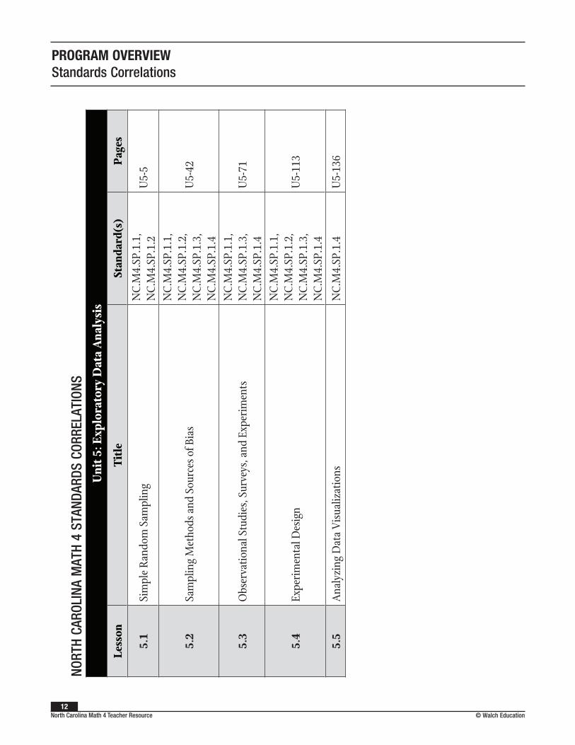
Unit 5: Exploratory Data AnalysisUnit 5 Resources . . . . . . . . . . . . . . . . . . . . . . . . . . . . . . . . . . . . . . . . . . . . . . . . . . . . . . . . . . . . . . . . . . . . U5-1
Lesson 5.1: Simple Random Sampling (NC.M4.SP.1.1, NC.M4.SP.1.2) . . . . . . . . . . . . . . . . . . . . U5-5Lesson 5.2: Sampling Methods and Sources of Bias
(NC.M4.SP.1.1, NC.M4.SP.1.2, NC.M4.SP.1.3, NC.M4.SP.1.4) . . . . . . . . . . . . . . . U5-42Lesson 5.3: Observational Studies, Surveys, and Experiments
(NC.M4.SP.1.1, NC.M4.SP.1.3, NC.M4.SP.1.4) . . . . . . . . . . . . . . . . . . . . . . . . . . . . . U5-71Lesson 5.4: Experimental Design (NC.M4.SP.1.1, NC.M4.SP.1.2, NC.M4.SP.1.3,
NC.M4.SP.1.4) . . . . . . . . . . . . . . . . . . . . . . . . . . . . . . . . . . . . . . . . . . . . . . . . . . . . . . . U5-113Lesson 5.5: Analyzing Data Visualizations (NC.M4.SP.1.4) . . . . . . . . . . . . . . . . . . . . . . . . . . . . U5-136
Answer Key . . . . . . . . . . . . . . . . . . . . . . . . . . . . . . . . . . . . . . . . . . . . . . . . . . . . . . . . . . . . . . . . . . . . . . . U5-163
Mid-Unit Assessment and Answer Key . . . . . . . . . . . . . . . . . . . . . . . . . . . . . . . . . . . . . . . . . . . . . . . MA-1
End-of-Unit Assessment and Answer Key . . . . . . . . . . . . . . . . . . . . . . . . . . . . . . . . . . . . . . . . . . . . . . EA-1
Unit 6: Probability DistributionsUnit 6 Resources . . . . . . . . . . . . . . . . . . . . . . . . . . . . . . . . . . . . . . . . . . . . . . . . . . . . . . . . . . . . . . . . . . . . U6-1
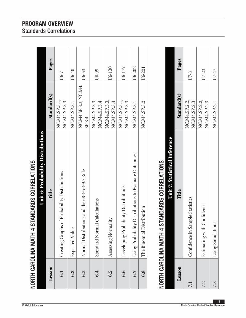
Lesson 6.1: Creating Graphs of Probability Distributions (NC.M4.SP.3.1, NC.M4.SP.3.3) . . . U6-7Lesson 6.2: Expected Value (NC.M4.SP.3.1) . . . . . . . . . . . . . . . . . . . . . . . . . . . . . . . . . . . . . . . . . . U6-40Lesson 6.3: Normal Distributions and the 68–95–99.7 Rule (NC.M4.SP.3.3, NC.M4.SP.3.4) . . . U6-63Lesson 6.4: Standard Normal Calculations (NC.M4.SP.3.3, NC.M4.SP.3.4) . . . . . . . . . . . . . . . U6-99Lesson 6.5: Assessing Normality (NC.M4.SP.3.3, NC.M4.SP.3.4) . . . . . . . . . . . . . . . . . . . . . . . U6-130Lesson 6.6: Developing Probability Distributions (NC.M4.SP.3.1, NC.M4.SP.3.3) . . . . . . . . U6-177Lesson 6.7: Using Probability Distributions to Evaluate Outcomes (NC.M4.SP.3.1) . . . . . . . U6-202Lesson 6.8: The Binomial Distribution (NC.M4.SP.3.2) . . . . . . . . . . . . . . . . . . . . . . . . . . . . . . . U6-221
Answer Key . . . . . . . . . . . . . . . . . . . . . . . . . . . . . . . . . . . . . . . . . . . . . . . . . . . . . . . . . . . . . . . . . . . . . . . U6-253
Extension ActivityPlaying Roulette (NC.M4.SP.3.1, NC.M4.SP.3.3, NC.M4.SP.3.4) . . . . . . . . . . . . . . . . . . . . . . . U6-261
Mid-Unit Assessment and Answer Key . . . . . . . . . . . . . . . . . . . . . . . . . . . . . . . . . . . . . . . . . . . . . . . MA-1
End-of-Unit Assessment and Answer Key . . . . . . . . . . . . . . . . . . . . . . . . . . . . . . . . . . . . . . . . . . . . . . EA-1

viii© Walch EducationNorth Carolina Math 4 Teacher Resource
PROGRAM OVERVIEWTable of Contents for Instructional Units
viii
Unit 7: Statistical InferenceUnit 7 Resources . . . . . . . . . . . . . . . . . . . . . . . . . . . . . . . . . . . . . . . . . . . . . . . . . . . . . . . . . . . . . . . . . . . . . U7-1
Lesson 7.1: Confidence in Sample Statistics (NC.M4.SP.2.2, NC.M4.SP.2.3) . . . . . . . . . . . . . . . U7-3 Lesson 7.2: Estimating with Confidence (NC.M4.SP.2.2, NC.M4.SP.2.3) . . . . . . . . . . . . . . . . . U7-23Lesson 7.3: Using Simulations (NC.M4.SP.2.1) . . . . . . . . . . . . . . . . . . . . . . . . . . . . . . . . . . . . . . . . U7-47
Answer Key . . . . . . . . . . . . . . . . . . . . . . . . . . . . . . . . . . . . . . . . . . . . . . . . . . . . . . . . . . . . . . . . . . . . . . . . U7-73
Mid-Unit Assessment and Answer Key . . . . . . . . . . . . . . . . . . . . . . . . . . . . . . . . . . . . . . . . . . . . . . . MA-1
End-of-Unit Assessment and Answer Key . . . . . . . . . . . . . . . . . . . . . . . . . . . . . . . . . . . . . . . . . . . . . . EA-1
Unit 8: ACT Prep: Complex Numbers, Matrices, and VectorsUnit 8 Resources . . . . . . . . . . . . . . . . . . . . . . . . . . . . . . . . . . . . . . . . . . . . . . . . . . . . . . . . . . . . . . . . . . . . U8-1
Lesson 8.1: Defining Complex Numbers, i, and i 2 (NC.M4.N.1.1) . . . . . . . . . . . . . . . . . . . . . . . . U8-7Lesson 8.2: Adding and Subtracting Complex Numbers (NC.M4.N.1.1) . . . . . . . . . . . . . . . . . U8-28Lesson 8.3: Multiplying Complex Numbers (NC.M4.N.1.2) . . . . . . . . . . . . . . . . . . . . . . . . . . . . U8-49Lesson 8.4: Finding the Complex Conjugate (NC.M4.N.1.2) . . . . . . . . . . . . . . . . . . . . . . . . . . . . U8-72Lesson 8.5: Operations with Matrices (NC.M4.N.2.1) . . . . . . . . . . . . . . . . . . . . . . . . . . . . . . . . . U8-93Lesson 8.6: Using Operations on Matrices (NC.M4.N.2.1) . . . . . . . . . . . . . . . . . . . . . . . . . . . . U8-120Lesson 8.7: Zero, Identity, Inverse, and Transformation Matrices (NC.M4.N.2.1) . . . . . . . . U8-149Lesson 8.8: Representing and Modeling with Vector Quantities (NC.M4.N.2.2) . . . . . . . . . . U8-185Lesson 8.9: Performing Operations on Vectors (NC.M4.N.2.2) . . . . . . . . . . . . . . . . . . . . . . . . U8-212
Answer Key . . . . . . . . . . . . . . . . . . . . . . . . . . . . . . . . . . . . . . . . . . . . . . . . . . . . . . . . . . . . . . . . . . . . . . . U8-245
Extension ActivityComputer Animation with Matrices (NC.M4.N.2.1) . . . . . . . . . . . . . . . . . . . . . . . . . . . . . . . . . . U8-253
Mid-Unit Assessment and Answer Key . . . . . . . . . . . . . . . . . . . . . . . . . . . . . . . . . . . . . . . . . . . . . . . MA-1
End-of-Unit Assessment and Answer Key . . . . . . . . . . . . . . . . . . . . . . . . . . . . . . . . . . . . . . . . . . . . . . EA-1

© Walch Education1
North Carolina Math 4 Teacher Resource
UNIT TK • UNIT TITLE TK
IntroductionThe North Carolina Math 4 Program is a complete set of materials developed around the North Carolina Standard Course of Study (NCSCOS) for Mathematics. Topics are built around accessible core curricula, ensuring that the North Carolina Math 4 Program is useful for striving students and diverse classrooms.
This program realizes the benefits of exploratory and investigative learning and employs a variety of instructional models to meet the learning needs of students with a range of abilities.
The North Carolina Math 4 Program includes components that support problem-based learning, instruct and coach as needed, provide practice, and assess students’ skills. Instructional tools and strategies are embedded throughout.
The program includes:
• More than 150 hours of lessons, addressing the eight units of North Carolina Math 4
• Essential Questions for each instructional topic
• Vocabulary
• Instruction and Guided Practice
• Problem-based Tasks and Coaching questions
• Step-by-step graphing calculator instructions for the TI-Nspire and the TI-83/84
• Station activities to promote collaborative learning and problem-solving skills
Purpose of Materials
The North Carolina Math 4 Program has been organized to coordinate with the North Carolina Math 4 content map and specifications from the NCSCOS. Each lesson includes activities that offer opportunities for exploration and investigation. These activities incorporate concept and skill development and guided practice, then move on to the application of new skills and concepts in problem-solving situations. Throughout the lessons and activities, problems are contextualized to enhance rigor and relevance.
PROGRAM OVERVIEW
Introduction to the Program

2© Walch EducationNorth Carolina Math 4 Teacher Resource
PROGRAM OVERVIEWIntroduction to the Program
This program includes all the topics addressed in the North Carolina Math 4 content map. These include:
• Building Mathematical Community with Parent Functions and Key Features
• Piecewise Functions, Composition of Functions, and Regression
• Logarithmic Functions
• Trigonometry
• Exploratory Data Analysis
• Probability Distributions
• Statistical Inference
• ACT Prep: Complex Numbers, Matrices, and Vectors
The eight Standards for Mathematical Practice are infused throughout:
1. Make sense of problems and persevere in solving them.
2. Reason abstractly and quantitatively.
3. Construct viable arguments and critique the reasoning of others.
4. Model with mathematics.
5. Use appropriate tools strategically.
6. Attend to precision.
7. Look for and make use of structure.
8. Look for and express regularity in repeated reasoning.
Structure of the Teacher Resource
The North Carolina Math 4 Custom Teacher Resource materials are completely reproducible. The Program Overview is the first section. This section helps you to navigate the materials, offers a comprehensive guide to Instructional Strategies for struggling readers, and shows the correlation between the NCSCOS for Mathematics and the North Carolina Math 4 course description.
The remaining materials focus on content, knowledge, and application of the eight units in the North Carolina Math 4 curriculum: Building Mathematical Community with Parent Functions and Key Features; Piecewise Functions, Composition of Functions, and Regression;

© Walch Education3
North Carolina Math 4 Teacher Resource
PROGRAM OVERVIEWIntroduction to the Program
Logarithmic Functions; Trigonometry; Exploratory Data Analysis; Probability Distributions; Statistical Inference; and ACT Prep: Complex Numbers, Matrices, and Vectors. The units in the North Carolina Math 4 Program are designed to be flexible so that you can mix and match activities as the needs of your students and your instructional style dictate.
Each unit includes a mid-unit assessment and an end-of-unit assessment. These enable you to gauge how well students have understood the material as you move from lesson to lesson and to differentiate as appropriate.

4© Walch EducationNorth Carolina Math 4 Teacher Resource
PROGRAM OVERVIEW
How Do Walch Integrated Mathematics Resources Address the Eight Standards for Mathematical Practice?Walch’s mathematics courses employ a problem-based model of instruction that supports and reinforces the eight Standards for Mathematical Practice. Although the following table focuses on Problem-Based Tasks, Walch’s full programs also include hundreds of additional problems in warm-ups and practices. The Implementation Guides for selected PBTs highlight SMPs to focus on during implementation and discussion.
CCSS Standards for Mathematical Practice
Relevant Attributes of Walch Integrated Math Resources
1 Make sense of problems and persevere in solving them.
Each lesson is built around a Problem-Based Task (PBT) that requires students to “make sense of problems and persevere in solving them.”
2 Reason abstractly and quantitatively.
Each PBT uses a meaningful real-world context that requires students to reason both abstractly about the situation/relationships and quantitatively about the values representing the elements and relationships.
3 Construct viable arguments and critique the reasoning of others.
Since the PBT provides opportunities for multiple problem-solving approaches and varied solutions, students are required to construct viable arguments to support their approach and answer. This, in turn, provides other students the opportunity to analyze and critique their classmates’ reasoning.
4 Model with mathematics.
Each PBT represents a real-world situation and requires students to model it with mathematics.
5 Use appropriate tools strategically.
PBTs require students to make choices about using appropriate tools, such as calculators, spreadsheets, graph paper, manipulatives, protractors, and compasses. The tasks do not prescribe specific tools, but instead provide opportunities for their use.
6 Attend to precision. The real-world contexts of the PBTs require students to be precise in their solutions, both in the ways that the solutions are stated, labeled, and explained, and in the degree of precision necessary given the context (e.g., tripling chili for a crowd vs. machining a part for an airplane engine).
7 Look for and make use of structure.
The PBTs present students with complicated scenarios that must be analyzed to discern patterns and significant mathematical features.
8 Look for and express regularity in repeated reasoning.
PBTs require multiple steps, providing opportunities for students to note repeated calculations, monitor their process, and continually evaluate reasonableness of intermediate results before arriving at a solution.
Correspondence to Standards for Mathematical Practice

© Walch Education5
North Carolina Math 4 Teacher Resource
PROGRAM OVERVIEW
All of the instructional units have common features. Each unit begins with a list of all the standards addressed in the lessons; Essential Questions; vocabulary (titled “Words to Know”); a list of recommended websites to be used as additional resources, and one or more conceptual activities.
Each lesson begins with a list of identified prerequisite skills that students need to have mastered in order to be successful with the new material in the upcoming lesson. This is followed by an introduction, key concepts, common errors/misconceptions, guided practice examples, a problem-based task with coaching questions and sample responses, and both print and digital practice.
All of the components are described below and on the following pages for your reference.
North Carolina Standard Course of Study for the Unit
All standards that are addressed in the entire unit are listed.
Essential Questions
These are intended to guide students’ thinking as they proceed through the lesson. By the end of each lesson, students should be able to respond to the questions.
Words to Know
A list of vocabulary terms that appear in the unit are provided as background information for instruction or to review key concepts that are addressed in the lesson. Each term is followed by a numerical reference to the first lesson in which the term is defined.
Recommended Resources
This is a list of websites that can be used as additional resources. Some websites are games; others provide additional examples and/or explanations. The links for these resources are live in the PDF version of the Teacher Resource. (Note: These website links will be monitored and repaired or replaced as necessary.) Each Recommended Resource is also accessible through Walch’s cloud-based Curriculum Engine Learning Object Repository as a separate learning object that can be assigned to students.
Conceptual Activities
Conceptual understanding serves as the foundation on which to build deeper understanding of mathematics. In an effort to build conceptual understanding of mathematical ideas and to provide more than procedural fluency and application, links to interactive open education and Desmos resources are included. (Note: These website links will be monitored and repaired or replaced as necessary.) These and many other open educational resources (OERs) are also accessible through the Learning Object Repository as separate objects that can be assigned to students.
Unit Structure

6© Walch EducationNorth Carolina Math 4 Teacher Resource
PROGRAM OVERVIEWUnit Structure
Warm-Up
Each warm-up takes approximately 5 minutes and addresses either prerequisite and critical-thinking skills or previously taught math concepts.
Warm-Up Debrief
Each debrief provides the answers to the warm-up questions, and offers suggestions for situations in which students might have difficulties. A section titled Connection to the Lesson is also included in the debrief to help answer students’ questions about the relevance of the particular warm-up activity to the upcoming instruction. Warm-Ups with debriefs are also provided in PowerPoint presentations.
Identified Prerequisite Skills
This list cites the skills necessary to be successful with the new material.
Introduction
This brief section gives a description of the concepts about to be presented and often contains some Words to Know.
Key Concepts
Provided in bulleted form, this instruction highlights the important ideas and/or processes for meeting the standard.
Graphing Calculator Directions
Step-by-step instructions for using a TI-Nspire and a TI-83/84 are provided whenever graphing calculators are referenced.
Common Errors/Misconceptions
This is a list of the common errors students make when applying Key Concepts. The list suggests what to watch for when students arrive at an incorrect answer or are struggling with solving the problems.
Scaffolded Practice (Printable Practice)
This set of 10 printable practice problems provides introductory level skill practice for the lesson. This practice set can be used during instruction time.

© Walch Education7
North Carolina Math 4 Teacher Resource
PROGRAM OVERVIEWUnit Structure
Guided Practice
This section provides step-by-step examples of applying the Key Concepts. The three to five examples are intended to aid during initial instruction, but are also for individuals needing additional instruction and/or for use during review and test preparation.
Enhanced Instructional PowerPoint (Presentation)
Each lesson includes an instructional PowerPoint presentation with the following components: Warm-Up, Key Concepts, and Guided Practice. Selected Guided Practice examples include GeoGebra applets. These instructional PowerPoints are downloadable and editable.
Problem-Based Task
This activity can serve as the centerpiece of a problem-based lesson, or it can be used to walk students through the application of the standard, prior to traditional instruction or at the end of instruction. The task makes use of critical-thinking skills.
Optional Problem-Based Task Coaching Questions with Sample Responses
These questions scaffold the task and guide students to solving the problem(s) presented in the task. They should be used at the discretion of the teacher for students requiring additional support. The Coaching Questions are followed by answers and suggested appropriate responses to the coaching questions. In some cases answers may vary, but a sample answer is given for each question.
Recommended Closure Activity
Students are given the opportunity to synthesize and reflect on the lesson through a journal entry or discussion of one or more of the Essential Questions.
Problem-Based Task Implementation Guide
This instructional overview, found with selected Problem-Based Tasks, highlights connections between the task and the lesson’s key concepts and SMPs. The Implementation Guide also offers suggestions for facilitating and monitoring, and provides alternative solutions.
Printable Practice (Sets A and B) and Interactive Practice (Set A)
Each lesson includes two sets of practice problems to support students’ achievement of the learning objectives. They can be used in any combination of teacher-led instruction, cooperative learning, or independent application of knowledge. Each Practice A is also available as an interactive Learnosity activity with Technology-Enhanced Items.
8© Walch EducationNorth Carolina Math 4 Teacher Resource
PROGRAM OVERVIEWUnit Structure
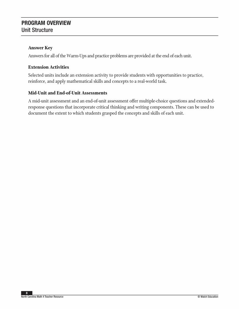
Answer Key
Answers for all of the Warm-Ups and practice problems are provided at the end of each unit.
Extension Activities
Selected units include an extension activity to provide students with opportunities to practice, reinforce, and apply mathematical skills and concepts to a real-world task.
Mid-Unit and End-of-Unit Assessments
A mid-unit assessment and an end-of-unit assessment offer multiple-choice questions and extended-response questions that incorporate critical thinking and writing components. These can be used to document the extent to which students grasped the concepts and skills of each unit.

© Walch Education9
North Carolina Math 4 Teacher Resource
Standards CorrelationsPROGRAM OVERVIEW
Each lesson in this North Carolina Math 4 program was written specifically to address the North Carolina Standard Course of Study (NCSCOS) for Mathematics. Each unit lists the standards covered in all the lessons, and each lesson lists the standards addressed in that particular lesson. In this section, you’ll find a comprehensive list mapping the lessons to the NCSCOS.
Guide to North Carolina Standard Course of Study AnnotationAs you use this program, you will come across a star symbol (★) included with the standards for some of the lessons and activities. This symbol is explained below.
Symbol: ★
Denotes: Modeling Standards
Modeling is best interpreted not as a collection of isolated topics but rather in relation to other standards. Making mathematical models is a Standard for Mathematical Practice, and specific modeling standards appear throughout the high school standards indicated by a star symbol (★).
From http://www.walch.com/CCSS/00003

10© Walch EducationNorth Carolina Math 4 Teacher Resource
PROGRAM OVERVIEWStandards Correlations
NORT
H CA
ROLI
NA M
ATH
4 ST
ANDA
RDS
CORR
ELAT
IONS
Uni
t 1: B
uild
ing
Mat
hem
atic
al C
omm
unit
y w
ith
Pare
nt F
unct
ions
and
Key
Fea
ture
s
Less
onTi
tle
Stan
dard
(s)
Page
s
1.1
Read
ing
and
Iden
tifyi
ng K
ey F
eatu
res o
f Rea
l-Wor
ld
Situ
atio
n G
raph
s N
C.M
3.F–
IF.4
★U
1-5
1.2
Tran
sfor
mat
ions
of P
aren
t Gra
phs
NC.
M3.
F–BF
.3U
1-54
1.3
Reco
gniz
ing
Odd
and
Eve
n Fu
nctio
ns
NC.
M3.
F–BF
.3U
1-92
NORT
H CA
ROLI
NA M
ATH
4 ST
ANDA
RDS
CORR
ELAT
IONS
Uni
t 2: P
iece
wis
e Fu
ncti
ons,
Com
posi
tion
of F
unct
ions
, and
Reg
ress
ion
Less
onTi
tle
Stan
dard
(s)
Page
s
2.1
Piec
ewise
, Ste
p, a
nd A
bsol
ute V
alue
Fun
ctio
ns
NC.
M4.
AF.
4.1,
N
C.M
4.A
F.4.
2U
2-5
2.2
Com
posi
tion
of F
unct
ions
N
C.M
4.A
F.1.
1U
2-33
2.3
Eval
uatin
g Co
mpo
site
Fun
ctio
ns in
Var
ious
For
ms
NC.
M4.
AF.
1.2
U2-
56
2.4
Line
ar, E
xpon
entia
l, an
d Q
uadr
atic
Reg
ress
ion
NC.
M4.
AF.
5.1
U2-
81
2.5
Ana
lyzi
ng R
esid
ual P
lots
N
C.M
4.A
F.5.
2U
2-11
2

© Walch Education11
North Carolina Math 4 Teacher Resource
PROGRAM OVERVIEWStandards Correlations
NORT
H CA
ROLI
NA M
ATH
4 ST
ANDA
RDS
CORR
ELAT
IONS
Uni
t 3: L
ogar
ithm
ic F
unct
ions
Less
onTi
tle
Stan
dard
(s)
Page
s
3.1
Inve
rses
of E
xpon
entia
l and
Log
arith
mic
Fun
ctio
ns
NC.
M4.
AF.
3.1
U3-
3
3.2
Com
mon
Log
arith
ms
NC.
M4.
AF.
3.1,
N
C.M
4.A
F.3.
2U
3-26
3.3
Nat
ural
Log
arith
ms
NC.
M4.
AF.
3.1,
N
C.M
4.A
F.3.
2U
3-48
3.4
Inte
rpre
ting
Loga
rith
mic
Mod
els
NC.
M4.
AF.
3.1,
N
C.M
4.A
F.3.
2,
NC.
M4.
AF.
3.3
U3-
81
3.5
Loga
rith
mic
Reg
ress
ion
NC.
M4.
AF.
5.1
U3-
111
NORT
H CA
ROLI
NA M
ATH
4 ST
ANDA
RDS
CORR
ELAT
IONS
Uni
t 4: T
rigo
nom
etry
Less
onTi
tle
Stan
dard
(s)
Page
s
4.1
Prov
ing
the
Fund
amen
tal P
ytha
gore
an Id
entit
y N
C.M
4.A
F.2.
1U
4-5
4.2
Prov
ing
the
Law
of S
ines
N
C.M
4.A
F.2.
2U
4-28
4.3
Prov
ing
the
Law
of C
osin
es
NC.
M4.
AF.
2.2
U4-
65
4.4
App
lyin
g th
e La
ws o
f Sin
es a
nd C
osin
es
NC.
M4.
AF.
2.2
U4-
91
4.5
Key
Fea
ture
s of T
rigo
nom
etri
c Fu
nctio
ns
NC.
M4.
AF.
2.3
U4-
123
4.6
Sinu
soid
al R
egre
ssio
n N
C.M
4.A
F.5.
1U
4-16
2
12© Walch EducationNorth Carolina Math 4 Teacher Resource
PROGRAM OVERVIEWStandards Correlations
NORT
H CA
ROLI
NA M
ATH
4 ST
ANDA
RDS
CORR
ELAT
IONS
Uni
t 5: E
xplo
rato
ry D
ata
Ana
lysi
s
Less
onTi
tle
Stan
dard
(s)
Page
s
5.1
Sim
ple
Rand
om S
ampl
ing
NC.
M4.
SP.1
.1,
NC.
M4.
SP.1
.2U
5-5
5.2
Sam
plin
g M
etho
ds a
nd S
ourc
es o
f Bia
s
NC.
M4.
SP.1
.1,
NC.
M4.
SP.1
.2,
NC.
M4.
SP.1
.3,
NC.
M4.
SP.1
.4
U5-
42
5.3
Obs
erva
tiona
l Stu
dies
, Sur
veys
, and
Exp
erim
ents
N
C.M
4.SP
.1.1
, N
C.M
4.SP
.1.3
, N
C.M
4.SP
.1.4
U5-
71
5.4
Expe
rim
enta
l Des
ign
NC.
M4.
SP.1
.1,
NC.
M4.
SP.1
.2,
NC.
M4.
SP.1
.3,
NC.
M4.
SP.1
.4
U5-
113
5.5
Ana
lyzi
ng D
ata
Vis
ualiz
atio
ns
NC.
M4.
SP.1
.4U
5-13
6
© Walch Education13
North Carolina Math 4 Teacher Resource
PROGRAM OVERVIEWStandards Correlations
NORT
H CA
ROLI
NA M
ATH
4 ST
ANDA
RDS
CORR
ELAT
IONS
Uni
t 6: P
roba
bilit
y D
istr
ibut
ions
Less
onTi
tle
Stan
dard
(s)
Page
s
6.1
Crea
ting
Gra
phs o
f Pro
babi
lity
Dis
trib
utio
ns
NC.
M4.
SP.3
.1,
NC.
M4.
SP.3
.3U
6-7
6.2
Expe
cted
Val
ue
NC.
M4.
SP.3
.1U
6-40
6.3
Nor
mal
Dist
ribut
ions
and
the 6
8–95
–99.
7 Ru
le
NC.
M4.
SP.3
.3, N
C.M
4.SP
.3.4
U6-
63
6.4
Stan
dard
Nor
mal
Cal
cula
tions
N
C.M
4.SP
.3.3
, N
C.M
4.SP
.3.4
U6-
99
6.5
Ass
essi
ng N
orm
ality
N
C.M
4.SP
.3.3
, N
C.M
4.SP
.3.4
U6-
130
6.6
Dev
elop
ing
Prob
abili
ty D
istr
ibut
ions
N
C.M
4.SP
.3.1
, N
C.M
4.SP
.3.3
U6-
177
6.7
Usi
ng P
roba
bilit
y D
istr
ibut
ions
to E
valu
ate
Out
com
es
NC.
M4.
SP.3
.1U
6-20
2
6.8
The
Bino
mia
l Dis
trib
utio
n N
C.M
4.SP
.3.2
U6-
221
NORT
H CA
ROLI
NA M
ATH
4 ST
ANDA
RDS
CORR
ELAT
IONS
Uni
t 7: S
tati
stic
al In
fere
nce
Less
onTi
tle
Stan
dard
(s)
Page
s
7.1
Conf
iden
ce in
Sam
ple
Stat
istic
s N
C.M
4.SP
.2.2
, N
C.M
4.SP
.2.3
U7-
3
7.2
Estim
atin
g w
ith C
onfid
ence
N
C.M
4.SP
.2.2
, N
C.M
4.SP
.2.3
U7-
23
7.3
Usi
ng S
imul
atio
ns
NC.
M4.
SP.2
.1U
7-47

14© Walch EducationNorth Carolina Math 4 Teacher Resource
PROGRAM OVERVIEWStandards Correlations
NORT
H CA
ROLI
NA M
ATH
4 ST
ANDA
RDS
CORR
ELAT
IONS
Uni
t 8: A
CT P
rep:
Com
plex
Num
bers
, Mat
rice
s, a
nd V
ecto
rs
Less
onTi
tle
Stan
dard
(s)
Page
s
8.1
Def
inin
g Co
mpl
ex N
umbe
rs, i
, and
i2 N
C.M
4.N
.1.1
U8-
7
8.2
Add
ing
and
Subt
ract
ing
Com
plex
Num
bers
N
C.M
4.N
.1.1
U8-
28
8.3
Mul
tiply
ing
Com
plex
Num
bers
N
C.M
4.N
.1.2
U8-
49
8.4
Find
ing
the
Com
plex
Con
juga
te
NC.
M4.
N.1
.2U
8-72
8.5
Ope
ratio
ns w
ith M
atri
ces
NC.
M4.
N.2
.1U
8-93
8.6
Usi
ng O
pera
tions
on
Mat
rice
s N
C.M
4.N
.2.1
U8-
120
8.7
Zero
, Ide
ntity
, Inv
erse
, and
Tra
nsfo
rmat
ion
Mat
rice
s N
C.M
4.N
.2.1
U8-
149
8.8
Repr
esen
ting
and
Mod
elin
g w
ith V
ecto
r Qua
ntiti
es
NC.
M4.
N.2
.2U
8-18
5
8.9
Perf
orm
ing
Ope
ratio
ns o
n V
ecto
rs
NC.
M4.
N.2
.2U
8-21
2

© Walch Education15
North Carolina Math 4 Teacher Resource
Conceptual ActivitiesPROGRAM OVERVIEW
Use these interactive open education and/or Desmos resources to build conceptual understanding of mathematical ideas. (Note: Activity links will be monitored and repaired or replaced as necessary.)
Unit 1
• Desmos. “Domain and Range Introduction.”
http://www.walch.com/ca/01049
In this activity, students practice finding the domain and range of piecewise functions. Students begin with an informal exploration of domain and range using a graph, and build up to representing the domain and range of piecewise functions using inequalities.
• Desmos. “Piecewise Functions 2019.”
http://www.walch.com/ca/01071
This activity introduces students to piecewise functions. Students will identify function types in a piecewise function and investigate the domains of piecewise functions.
• Desmos. “Polygraph: Absolute Value.”
http://www.walch.com/ca/01050
This activity is designed to spark vocabulary-rich conversations about transformations of the absolute value parent function. Key vocabulary terms that may appear in student questions include translation, shift, slide, dilation, stretch, horizontal, vertical, and reflect.
• Desmos. “Polygraph: Parent Functions.”
http://www.walch.com/ca/01051
This activity is designed to spark vocabulary-rich conversations about graphs of parent functions. Key vocabulary terms that may appear in student questions include increasing, decreasing, linear, quadratic, cubic, absolute value, exponential, logarithmic, rational, radical, axis, intercept, and coordinate.
• Desmos. “Polygraph: Piecewise Functions.”
http://www.walch.com/ca/01052
This activity is designed to spark vocabulary-rich conversations about piecewise functions. Key vocabulary terms that may appear in student questions include piecewise, continuous, and interval.

16© Walch EducationNorth Carolina Math 4 Teacher Resource
PROGRAM OVERVIEWConceptual Activities
• Desmos. “Polygraph: Twelve Functions.”
http://www.walch.com/ca/01053
This activity is designed to spark vocabulary-rich conversations about various functions. Key vocabulary terms that may appear in student questions include linear, quadratic, exponential, cubic, absolute value, rational, radical, sinusoid, and step.
• Desmos. “Writing Rules: Linear, Quadratic, and Exponential.”
http://www.walch.com/ca/01047
In this activity, students have an opportunity to deepen their understanding of linear, quadratic, and exponential functions by making connections between their tables, graphs, and equations.
Unit 2
• Desmos. “Composing Functions Exploration.”
http://www.walch.com/ca/01070
This exploration offers practice with composing functions, dives deeper into properties of composition, and provides an introduction to inverse functions by encouraging students to consider compositions that result in the line y = x.
• Desmos. “LEGO Prices.”
http://www.walch.com/ca/01012
Use the concept of linear regression to predict the cost of a LEGO set with x pieces. (This activity does NOT use the calculator, just the concept. Participants draw the line on the graph, and Desmos calculates the equation.)
• Desmos. “Polygraph: Piecewise Functions.”
http://www.walch.com/ca/01052
This activity is designed to spark vocabulary-rich conversations about piecewise functions. Key vocabulary terms that may appear in student questions include piecewise, continuous, and interval.
• Desmos. “Polygraph: Twelve Functions.”
http://www.walch.com/ca/01053
This activity is designed to spark vocabulary-rich conversations about various functions. Key vocabulary terms that may appear in student questions include linear, quadratic, exponential, cubic, absolute value, rational, radical, sinusoid, and step.
© Walch Education17
North Carolina Math 4 Teacher Resource
PROGRAM OVERVIEWConceptual Activities
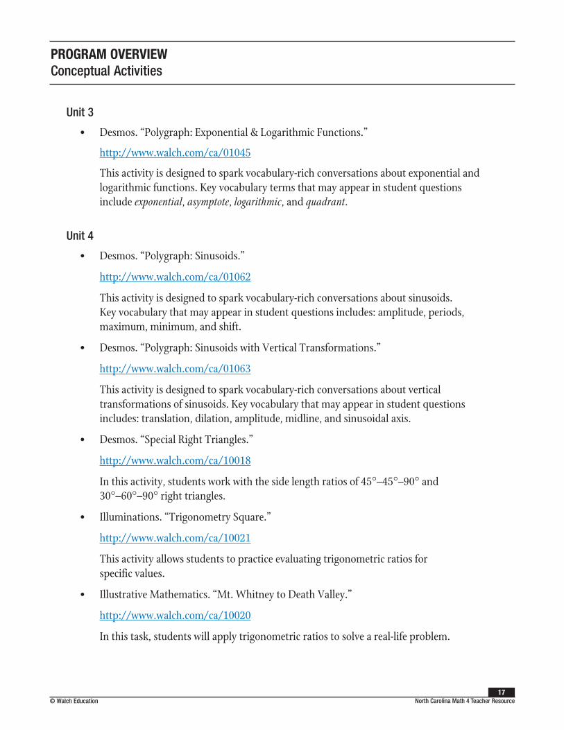
Unit 3
• Desmos. “Polygraph: Exponential & Logarithmic Functions.”
http://www.walch.com/ca/01045
This activity is designed to spark vocabulary-rich conversations about exponential and logarithmic functions. Key vocabulary terms that may appear in student questions include exponential, asymptote, logarithmic, and quadrant.
Unit 4
• Desmos. “Polygraph: Sinusoids.”
http://www.walch.com/ca/01062
This activity is designed to spark vocabulary-rich conversations about sinusoids. Key vocabulary that may appear in student questions includes: amplitude, periods, maximum, minimum, and shift.
• Desmos. “Polygraph: Sinusoids with Vertical Transformations.”
http://www.walch.com/ca/01063
This activity is designed to spark vocabulary-rich conversations about vertical transformations of sinusoids. Key vocabulary that may appear in student questions includes: translation, dilation, amplitude, midline, and sinusoidal axis.
• Desmos. “Special Right Triangles.”
http://www.walch.com/ca/10018
In this activity, students work with the side length ratios of 45°–45°–90° and 30°–60°–90° right triangles.
• Illuminations. “Trigonometry Square.”
http://www.walch.com/ca/10021
This activity allows students to practice evaluating trigonometric ratios for specific values.
• Illustrative Mathematics. “Mt. Whitney to Death Valley.”
http://www.walch.com/ca/10020
In this task, students will apply trigonometric ratios to solve a real-life problem.

18© Walch EducationNorth Carolina Math 4 Teacher Resource
PROGRAM OVERVIEWConceptual Activities
Unit 5
• Amanda Walker on American Statistical Association’s STatistics Education Web (STEW). “The Egg Roulette Game.”
http://www.walch.com/ca/01072
This activity walks students through playing and analyzing the outcomes of a game based on random sampling. Note: Scroll down to the “Grades 9 – 12+” section of the page to find the game.
• Heather Pierce. “Sampling methods.”
http://www.walch.com/ca/01073
This applet provides simple, clear illustrations for four sampling methods.
Unit 6
• Illustrative Mathematics. “Do You Fit In This Car?”
http://www.walch.com/ca/01065
This task allows students to use the normal curve as a model for a distribution of heights in a population. Students must calculate population percentages from given statistics.
• Illustrative Mathematics. “Fred’s Fun Factory.”
http://www.walch.com/ca/01066
This task gives students the opportunity to use expected value in a decision-making process. While it is possible to solve this problem by analyzing a discrete probability model, the large number of cases make this method somewhat challenging.
• Illustrative Mathematics. “SAT Scores.”
http://www.walch.com/ca/01067
This task encourages students to view the empirical rule as an estimation tool to reinforce understanding that the normal distribution is an only an approximation of the true distribution. Students may apply the empirical rule without needing a calculator.
• Illustrative Mathematics. “Should We Send Out a Certificate?”
http://www.walch.com/ca/10006
This task allows students to practice calculating normal distributions and further encourages them to draw conclusions from their results based on the properties of normal distributions. Students will communicate their findings in a narrative form within the context of the problem rather than reporting a simple computed number.

© Walch Education19
North Carolina Math 4 Teacher Resource
PROGRAM OVERVIEWConceptual Activities
• Illustrative Mathematics. “Sounds Really Good! (sort of...).”
http://www.walch.com/ca/01068
This task gives students the opportunity to work more with expected value. Students will compute and interpret an expected value, and use this information in a decision-making process. Students will communicate their findings in the form of a letter, encouraging them to conceptualize their understanding of the problem in context in non-technical terms.
Unit 8
• Desmos. “Intro to Vectors 2019.”
http://www.walch.com/ca/01069
This activity introduces vectors in the coordinate plane through a series of short activities. Students will find vector magnitudes, as well as add, subtract, and scalar multiply vectors.
• Illustrative Mathematics. “Computations with Complex Numbers.”
http://www.walch.com/ca/10004
Students will practice operations on complex numbers using the fact that i2 = –1. Encourage students to examine the structure of each expression and look for shortcuts (SMP 7), as this task allows for the shortening of some tedious calculations. This task is also an excellent candidate for comparison of different approaches to the same problem.
20© Walch EducationNorth Carolina Math 4 Teacher Resource
UNIT TK • UNIT TITLE TK
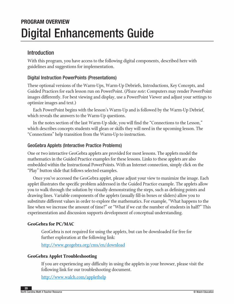
IntroductionWith this program, you have access to the following digital components, described here with guidelines and suggestions for implementation.
Digital Instruction PowerPoints (Presentations)
These optional versions of the Warm-Ups, Warm-Up Debriefs, Introductions, Key Concepts, and Guided Practices for each lesson run on PowerPoint. (Please note: Computers may render PowerPoint images differently. For best viewing and display, use a PowerPoint Viewer and adjust your settings to optimize images and text.)
Each PowerPoint begins with the lesson’s Warm-Up and is followed by the Warm-Up Debrief, which reveals the answers to the Warm-Up questions.
In the notes section of the last Warm-Up slide, you will find the “Connections to the Lesson,” which describes concepts students will glean or skills they will need in the upcoming lesson. The “Connections” help transition from the Warm-Up to instruction.
GeoGebra Applets (Interactive Practice Problems)
One or two interactive GeoGebra applets are provided for most lessons. The applets model the mathematics in the Guided Practice examples for these lessons. Links to these applets are also embedded within the Instructional PowerPoints. With an Internet connection, simply click on the “Play” button slide that follows selected examples.
Once you’ve accessed the GeoGebra applet, please adjust your view to maximize the image. Each applet illustrates the specific problem addressed in the Guided Practice example. The applets allow you to walk through the solution by visually demonstrating the steps, such as defining points and drawing lines. Variable components of the applets (usually fill-in boxes or sliders) allow you to substitute different values in order to explore the mathematics. For example, “What happens to the line when we increase the amount of time?” or “What if we cut the number of students in half?” This experimentation and discussion supports development of conceptual understanding.
GeoGebra for PC/MAC
GeoGebra is not required for using the applets, but can be downloaded for free for further exploration at the following link:
http://www.geogebra.org/cms/en/download
GeoGebra Applet Troubleshooting
If you are experiencing any difficulty in using the applets in your browser, please visit the following link for our troubleshooting document.
http://www.walch.com/applethelp
Digital Enhancements GuidePROGRAM OVERVIEW

© Walch Education21
North Carolina Math 4 Teacher Resource
PROGRAM OVERVIEWDigital Enhancements Guide
Curriculum Engine Item Bank
Walch’s Curriculum Engine comes loaded with thousands of curated learning objects that can be used to build formative and summative assessments as well as practice worksheets. District leaders and teachers can search for items by standard and create assessments or worksheets in minutes using the three-step assessment builder.
For more information about the Curriculum Engine Item Bank, or for additional support, please contact Customer Service at (800) 341-6094 or [email protected].

22© Walch EducationNorth Carolina Math 4 Teacher Resource
Standards for Mathematical Practice Implementation Guide
PROGRAM OVERVIEW
IntroductionThe eight Standards for Mathematical Practice describe features of lesson design, teaching pedagogy, and student actions that will lead to a true conceptual understanding of the mathematics standards. Walch’s lessons, practice problems, and Problem-Based Tasks lend themselves to teaching through this framework. When the Walch resources are combined with high-level questioning and engaging teacher decisions in the classroom, it will lead to high-level math instruction and student achievement.
Here is a brief description of the SMPs and how they can be applied in the classroom:
SMP 1: Make sense of problems and persevere in solving them.
Students will read, interpret, and understand complicated mathematical and real-world problems, and they will be willing to try multiple methods with the ultimate goal of determining the correct answer. Strategies such as annotation and student discourse can lead to improvement on this standard. Presenting students with higher-level problems is essential to ensuring students achieve maximum understanding. Teacher prompts that can enhance this standard include:
• What is the problem asking you to solve?
• What are some (other) strategies you could use to solve this problem?
• Compare your answer with a classmate’s answer. Who is correct? Why?
SMP 2: Reason abstractly and quantitatively.
Mathematical reasoning with numbers and variables is essential to understanding the connections among the standards. Students must be able to discover and formalize general rules using numbers and variables, and apply them to determine numerical quantities in other situations. Teacher prompts that can enhance this standard include:
• Substitute realistic numbers into the situation.
• What operation/strategy would you use?
• Will your strategy work for any number?
• For which categories of numbers (negative integers, all real numbers, etc.) will your strategy work?

© Walch Education23
North Carolina Math 4 Teacher Resource
PROGRAM OVERVIEWStandards for Mathematical Practice Implementation Guide
SMP 3: Construct viable arguments and critique the reasoning of others.
Many students are most concerned with the “what” aspects of mathematics, i.e. “what” do we do or “what” is the answer. However, math educators must develop the “why” of mathematics. Students must learn to question algorithms, challenge answers, and justify their reasoning in order to truly understand the concepts behind their answers. Teacher prompts that can enhance this standard include:
• How did you determine your answer?
• Why did you choose that strategy?
• Defend your answer based on a real-world situation.
SMP 4: Model with mathematics.
An important goal of mathematics instruction is for students to be able to apply mathematics to the world around them. Students should be able to link a real problem to a mathematical concept, identify quantities that are modeled well with mathematics, and use mathematics to find a solution. Emphasizing this standard will help students represent and interpret information using physical, visual, and abstract models. Encourage students to use any or all of their learning experiences to gain a deep and flexible understanding of mathematics. Teacher prompts that can enhance this standard include:
• Can you represent this situation with a visual model?
• How will it help you solve the problem?
• What information is needed to solve this problem?
• Is there another way to solve this problem?
• While working to solve this problem, what do you notice/wonder?
SMP 5: Use appropriate tools strategically.
There are many available tools suitable for mathematics, such as calculators, manipulatives, formulas, rulers, computers, and developed mathematical strategies. Choosing and using the correct tool to work through a problem is an important skill for mathematicians. Teacher prompts that can enhance this standard include:
• Can you graph this equation in the calculator to see a relationship?
• What formula or strategy might help you determine the answer to this question?
• How can you represent the situation using handheld tools (rulers, protractors, etc.) to determine an answer?

24© Walch EducationNorth Carolina Math 4 Teacher Resource
PROGRAM OVERVIEWStandards for Mathematical Practice Implementation Guide
SMP 6: Attend to precision.
When using mathematics to solve problems, an answer can be considered correct only if it is sufficiently precise and accurate for the situation to which it pertains. When applying mathematics, it is vital to clearly define the question, the reasoning, the answer, and the explanation. Vocabulary, units, numerical responses, and pictures must be represented precisely in questions and answers to ensure that the mathematical solutions represent the true answer to a question. Teacher prompts that can enhance this standard include:
• What does your answer represent in a real-world context?
• Is your answer reasonable based on your initial estimate?
• What units of measure help describe your numerical answer?
SMP 7: Look for and make use of structure.
Structure, whether geometric, algebraic, statistical, or numerical, is an important aspect of mathematical reasoning that students often overlook. Teachers often explicitly refer to geometric and other visual structures as explanations of mathematical concepts, but algebraic and numerical structures can often be just as important in analyzing and interpreting mathematical situations. These structures yield clues as to the meaning of expressions, equations, graphs, and other representations. As students interpret these structures, they will gain a greater understanding of the mathematical concepts. Teacher prompts that can enhance this standard include:
• What do the characteristics of the graph tell us about the situation?
• What do each of the variables and numbers in the equation/formula represent?
• How are these situations the same and different based on their representations?
SMP 8: Look for and express regularity in repeated reasoning.
Just as patterns appear in real life, patterns appear throughout the subject of mathematics. Recognizing and applying these patterns, and applying the reasoning contained within, is one of the most important skills teachers can instill in their students. Rather than teaching isolated algorithms to determine answers, have students discover relationships, create their own algorithms, and apply the reasoning to other situations. These skills can be applied throughout their education and will enrich their lives after high school. Teacher prompts that can enhance this standard include:
• What relationship do you notice in the graph/table/numbers?
• Why did you choose to use this process to solve this word problem/equation?
• How can you apply this process in other situations?

© Walch Education25
North Carolina Math 4 Teacher Resource
Instructional StrategiesPROGRAM OVERVIEW
Ensuring Access for All StudentsIntroduction
The increased focus on literacy in math instruction can help some students navigate mathematical contexts, but for struggling readers, it can further complicate calculations. English language learners struggle to master difficult mathematical concepts while simultaneously processing a new language. Students with learning and behavioral disabilities struggle with the math concepts in their own contexts. This is where teachers and the strategies they select for their classrooms become essential.
The strategies presented here can help all students succeed in math, literacy, school, and, ultimately, in life. These instructional strategies provide teachers with a wide range of instructional support to aid English as a Second Language (ESL) students, students with disabilities (SWD), and struggling readers. These strategies provide support for the Mathematics Standards and the Standards of Mathematical Practice (SMP), English Language Development (ELD) Standards, English Language Arts Standards, and WIDA English Language Development Standards.
Within each lesson throughout this course, you will find suggested instructional strategies. These instructional strategies are research-based strategies and best practices that work well for all students.
The instructional strategies detailed here fall into four main categories: Literacy, Mathematical Discourse, Annotation, and Graphic Organizers. These strategies provide teachers with research-based strategies to address the needs of all students.
• Close Reading• Text to Speech• Concept-Picture- Word Wall• Novel Ideas
• Reverse Annotation
• CUBES Protocol
• Frayer Model
• Table of Values
• Sentence Starters
• Small Group DiscussionLiteracy
Strategies
MathematicalDiscourseStrategies
AnnotationStrategies
GraphicOrganizerStrategies
Source
• WIDA: https://www.wida.us/standards/eld.aspx

26© Walch EducationNorth Carolina Math 4 Teacher Resource
PROGRAM OVERVIEWInstructional Strategies: Literacy
Understanding the Language of Mathematics: Literacy Mathematics has its own language consisting of words, notations, formulas, and visuals. In education, the language of mathematics is often regarded solely in the context of word problems and articles. This neglects the vocabulary and other mathematical representations students must be able to interpret. The strategies presented here help students navigate the language of mathematics so that they can understand text and feel confident speaking in and listening to mathematical discussions. For students with disabilities, the stress on repetition and different representations in this approach is essential to their ability to grasp the math concepts. For ESL students, repetition and different representations can strip out some of the English language barriers to understanding the language of mathematics, as well as provide multiple means of accessing the content. Literacy strategies include Close Reading, Text-to-Speech, Concept-Picture-Word Walls, and Novel Ideas.
LiteracyStrategies
MathematicalDiscourseStrategies
AnnotationStrategies
GraphicOrganizerStrategies

© Walch Education27
North Carolina Math 4 Teacher Resource
PROGRAM OVERVIEWInstructional Strategies: Literacy
Literacy Strategies
??Close Reading with Guiding Questions
What is Close Reading with Guiding Questions?
Close Reading with Guiding Questions is a process that allows students to preview mathematical reading and problems by answering questions related to the text in advance and reviewing their responses during and/or after reading. Multiple reading protocols can be used in conjunction with guiding questions to enhance their effectiveness.
How do you implement Close Reading with Guiding Questions in the classroom?
When utilizing a textbook, task, or article in a math class, literacy struggles are often a strong barrier to entry into the mathematical ideas. Asking students to answer accessible questions before and/or as they read can lead them to the key information.
Prior to implementation, the teacher should determine the most important information students need to obtain from a text, whether it is a math problem to solve, a task to complete, or an informational lesson or article to read. Then, the teacher should come up with some questions to guide students before they read. These questions can:
• assess and relate prior knowledge
• define key vocabulary words
• discuss non-mathematical concepts in the text
The teacher should also prepare some questions to guide students as they read. These questions can:
• point out key concepts within the text
• relate the text and concepts to future learning
• assist students in identifying key facts in the text
• highlight the importance of text features (graphics, headings, etc.) in the text
To ensure the questions are accessible for students and to encourage reflection and debate after reading, many of these questions should be designed as either “True/False” or “Always True/Sometimes True/Never True.” Students can represent their reasoning for their answer in writing, numbers, or graphic/pictorial representations. Students should complete the guiding questions and reading individually, with discussion to follow.
After students complete the reading, they should be given some time to individually evaluate their initial answers. Then, in partners or in groups, they can discuss their answers and come to final conclusions that will help them find the important information initially identified by the teacher. After deciphering the text through close reading, students will be able to complete the given activity.

28© Walch EducationNorth Carolina Math 4 Teacher Resource
PROGRAM OVERVIEWInstructional Strategies: Literacy
When would I use Close Reading with Guiding Questions in the classroom?
Close Reading with Guiding Questions can be used for any activity in which literacy could be a barrier to learning or demonstrating mastery of mathematical concepts. The number of questions and length of the discussions can be altered based on the length, importance, and difficulty of the text and concept. As students become more accustomed to mathematical literacy, the text complexity can be increased, but the adherence to close reading strategies must be maintained to ensure students can access the mathematical concepts. The length of time spent on the literacy aspect can be shortened as students become more skilled, but the questioning and discussions must occur to ensure students are properly interpreting the text in the mathematical context.
How can I use Close Reading with Guiding Questions with students needing additional support?
For struggling readers, including ESLs, Close Reading with Guiding Questions can help make an intimidating lesson, word problem, or task much more accessible. Questions focusing more on Tier 2 and Tier 3 vocabulary, text features, and real-world concepts can help struggling readers relate to the text and learn how to decipher the text in context. Discussions around the questions will help students grasp the math concepts.
Allowing struggling readers to explain their answers using words, numbers, or graphics/pictures ensures that they can express their opinion and rationale despite a potential lack of vocabulary. Through these representations and the ensuing discussion, students will begin to learn the necessary vocabulary to be successful.
What other standards does Close Reading with Guiding Questions address?
Standards of Mathematical Practice:
• SSMP.1
• SSMP.6
WIDA English Language Development Standards:
• ELD Standard 3
Language Arts Standards:
• ELA–LITERACY.WHST.9–10.4
• ELA–LITERACY.WHST.9–10.9
• ELA–LITERACY.SL.9–10.4
• ELA–LITERACY.RST.9–10.3
• ELA–LITERACY.RST.9–10.4
• ELA–LITERACY.RST.9–10.7

© Walch Education29
North Carolina Math 4 Teacher Resource
PROGRAM OVERVIEWInstructional Strategies: Literacy
Sources
• Anne Adams, Jerine Pegg, and Melissa Case. “Anticipation Guides: Reading for Mathematics Understanding.”
https://www.nctm.org/Publications/mathematics-teacher/2015/Vol108/Issue7/Anticipation-Guides-Reading-for-Mathematics-Understanding/
• Diane Staehr Fenner and Sydney Snyder. “Creating Text Dependent Questions for ELLs: Examples for 6th to 8th Grade.”
http://www.colorincolorado.org/blog/creating-text-dependent-questions-ells-examples-6th-8th-grade-part-3

30© Walch EducationNorth Carolina Math 4 Teacher Resource
PROGRAM OVERVIEWInstructional Strategies: Literacy
Literacy Strategies Text-to-Speech Technology
What is Text-to-Speech Technology?
Text-to-Speech Technology is an adaptive technology that reads text aloud from a text source for students. It is usually accessed through an application or program on a computer, smartphone, or tablet. Some new programs utilize Mathematical Markup Language (MathML) to read mathematical notation in a common, understandable manner for students. Many programs also highlight the words and notation on the screen as the audio plays, which helps students relate the written representation to the words they hear. The use of Text-to-Speech Technology allows students who struggle with literacy to hear the words and notation and access the text in a different way.
How do you implement Text-to-Speech Technology?
A classroom community focused on everyone’s learning and a growth mindset is the first step in implementing Text-to-Speech Technology. One of the main barriers to implementation is encouraging students to use the program. Once they do, they will realize how the audio can help them understand the difficult mathematical texts and interpret the math content within them. After students realize the benefits of Text-to-Speech Technology, it can become part of the regular routine for group and independent work.
The use of headphones can be very important for effective use of Text-to-Speech Technology. Students can use the technology to listen to lessons and texts at their own pace. Extra noise from other students working or other students listening at different paces can confuse students attempting to use Text-to-Speech Technology, and headphones can help mitigate these distractions. Many teachers are nervous about the potential disruption headphones can cause in class. However, well-managed use of headphones can help students successfully utilize the technology to learn.
When would I use Text-to-Speech Technology in the classroom?
Text-to-Speech Technology can be used at any time throughout the year, and if the program speaks in MathML, it can be used with any lesson. Without MathML, effective use could be limited to word problems without unusual notation. For example, if x2 is read as “x-two” instead of “x-squared” or “x to the second power,” that could confuse students more.
During a lesson or small group discussion, Text-to-Speech Technology could detract from students’ ability to listen, question, and process information. However, during warm-ups, independent work, or assessments, Text-to-Speech Technology can help students process the information and access the activity. It can become a routine for students to automatically listen to the question, problem, or directions first, and then attempt the activity.
© Walch Education31
North Carolina Math 4 Teacher Resource
PROGRAM OVERVIEWInstructional Strategies: Literacy
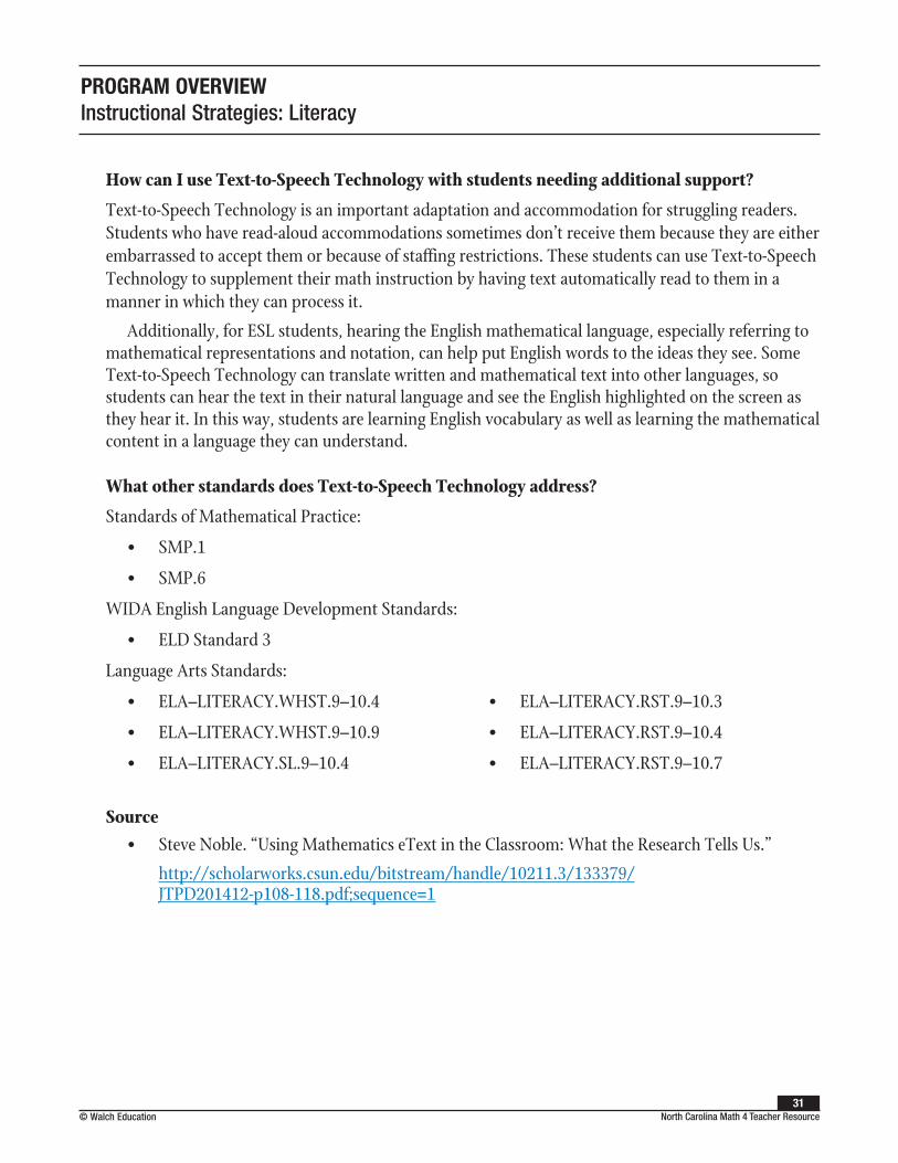
How can I use Text-to-Speech Technology with students needing additional support?
Text-to-Speech Technology is an important adaptation and accommodation for struggling readers. Students who have read-aloud accommodations sometimes don’t receive them because they are either embarrassed to accept them or because of staffing restrictions. These students can use Text-to-Speech Technology to supplement their math instruction by having text automatically read to them in a manner in which they can process it.
Additionally, for ESL students, hearing the English mathematical language, especially referring to mathematical representations and notation, can help put English words to the ideas they see. Some Text-to-Speech Technology can translate written and mathematical text into other languages, so students can hear the text in their natural language and see the English highlighted on the screen as they hear it. In this way, students are learning English vocabulary as well as learning the mathematical content in a language they can understand.
What other standards does Text-to-Speech Technology address?
Standards of Mathematical Practice:
• SMP.1
• SMP.6
WIDA English Language Development Standards:
• ELD Standard 3
Language Arts Standards:
• ELA–LITERACY.WHST.9–10.4
• ELA–LITERACY.WHST.9–10.9
• ELA–LITERACY.SL.9–10.4
• ELA–LITERACY.RST.9–10.3
• ELA–LITERACY.RST.9–10.4
• ELA–LITERACY.RST.9–10.7
Source • Steve Noble. “Using Mathematics eText in the Classroom: What the Research Tells Us.”
http://scholarworks.csun.edu/bitstream/handle/10211.3/133379/JTPD201412-p108-118.pdf;sequence=1

32© Walch EducationNorth Carolina Math 4 Teacher Resource
PROGRAM OVERVIEWInstructional Strategies: Literacy
Literacy Strategies more> thanConcept-Picture-Word Wall
What is a Concept-Picture-Word Wall?
A Concept-Picture-Word Wall is a classroom display, often a bulletin board or a set of posters, that exposes students to important vocabulary words they will use in math class.
Posting vocabulary words in class helps reinforce the words students will see in textbooks, videos, websites, and test questions on math concepts. These Tier 3 vocabulary words are often not used in everyday language, and the exposure to the words visually through Concept-Picture-Word Walls can help students connect them to the math content.
How do you implement Concept-Picture-Word Walls in the classroom?
Just seeing the vocabulary on a Concept-Picture-Word Wall by itself will help students; more importantly, referring to the words as the teacher uses them in class helps students connect the visual to the application. A simple gesture to the wall makes a very explicit reference to the word as it is used and allows students to connect the unfamiliar word to its meaning in context. Additionally, students can be taught to refer to the wall as they use the words in class, and they can be asked to make sure they say at least 3 words from the wall during each class period in small-group discourse or as answers to whole-class questions. The comfort gained from using these Tier 3 words will help students to use appropriate math vocabulary while solving problems and will help students connect concepts more explicitly.
Postings on the Concept-Picture-Word Wall can be arranged strategically to connect concepts, units of study, or groups of words where appropriate. Having three sections of the Concept-Picture-Word Wall—for example, an “In the Future” section, a “Live in the Present” section, and a “Remember the Past” section–—can help students see and remember the vocabulary throughout the entire course. Even without regular use of some words, just seeing the words before a unit can help instill a familiarity with the vocabulary. Leaving the words on the Concept-Picture-Word Wall after a unit is taught can help students connect “old” concepts to the current lesson and ensure that students still have access to the vocabulary.
When would I use Concept-Picture-Word Walls in the classroom?
Concept-Picture-Word Walls can be used for the entire year. The actual words might have to change, or at least be moved to different areas of the Concept-Picture-Word wall. The more exposure students have to the words, the more familiar and comfortable they will become. The constant exposure to the math context is beneficial for students throughout the entire course, especially for words with multiple meanings (bias, tangent, etc.) that could exist as Tier 2 words in everyday conversation but are Tier 3 words in the math classroom.

© Walch Education33
North Carolina Math 4 Teacher Resource
PROGRAM OVERVIEWInstructional Strategies: Literacy
How can I use Concept-Picture-Word Walls with students needing additional support?
For all students learning mathematics, knowing and using the math vocabulary is often a major barrier. This is a problem especially for ESL students, who are learning the English language along with math content. If teachers try to simplify the words too much for students, it does them a disservice as they seek out information from other teachers, textbooks, and online sources that use the proper vocabulary. Most tests, especially state tests, will expect students to have knowledge of the Tier 3, math-specific vocabulary. The more students see these words, the more familiarity they will have when they apply them.
Concept-Picture-Word Walls can also be written in multiple languages. Especially for students who are on-grade-level in their native language, a multi-lingual Concept-Picture-Word Wall can help students connect the content they already know in another language to the English vocabulary necessary for success on English-language math activities and tests.
This website can help you get started on an English-Spanish Concept-Picture-Word Wall: http://math2.org/math/spanish/eng-spa.htm
What other standards do Concept-Picture-Word Walls address?
Standards of Mathematical Practice:
• SMP.1
• SMP.6
WIDA English Language Development Standards:
• ELD Standard 3
Language Arts Standards:
• ELA–LITERACY.WHST.9–10.4
• ELA–LITERACY.WHST.9–10.9
• ELA–LITERACY.SL.9–10.4
• ELA–LITERACY.RST.9–10.3
• ELA–LITERACY.RST.9–10.4
• ELA–LITERACY.RST.9–10.7
Source
• Janis M. Harmon, Karen D. Wood, Wanda B. Hedrick, Jean Vintinner, and Terri Willeford. “Interactive Word Walls: More Than Just Reading the Writing on the Walls.”
http://citeseerx.ist.psu.edu/cdownload;jsessionid=A250AF8A870B13B40B2934 BA515FEC9?doi=10.1.1.690.6740&rep=rep1&type=pdf

34© Walch EducationNorth Carolina Math 4 Teacher Resource
PROGRAM OVERVIEWInstructional Strategies: Literacy
Literacy Strategies !!!Novel Ideas
What is Novel Ideas?
Novel Ideas is a classroom activity that explores students’ understanding of important Tier 2 vocabulary words they will use in math class. Instead of asking students to look up vocabulary words in the dictionary, Novel Ideas allows students to have conversations with their peers about vocabulary words in class. This reinforces the mathematical vocabulary students will see in textbooks, videos, websites, and test questions. These Tier 2 vocabulary words are often used in everyday language, but have specific meaning in mathematics. Exposure to the words through Novel Ideas can help students connect them to the math content.
How do you implement Novel Ideas in the classroom?
While building a rich representation of math content words and connecting the words to other words and concepts has inherent merit, it is more important to consider that pre-teaching the words before they are used in class helps students connect to the application. The understanding gained from discussing these Tier 2 words will help students apply them in a mathematical context to solve problems and connect concepts.
Here is a step-by-step process for implementing Novel Ideas:
1. Students separate into groups of four.
2. Students copy the teacher generated prompt/sentence starters and number their papers 1–8.
3. One student offers an idea, another echoes it, and all write it down.
4. After three minutes, students draw a line under the last item in the list.
5. All students stand, and the teacher calls one student from a group to read the group’s list.
6. The student starts by reading the prompt/sentence starters, “We think a ______ called ______ may be about … ,” and then adds whatever ideas the team has agreed on.
7. The rest of the class must pay attention because after the first group has presented all their ideas, the teacher asks them to sit down and calls on a student from another team to add that team’s “novel ideas only.” Ideas that have already been presented cannot be repeated.
8. As teams complete their turns and sit down, each seated student should record novel ideas from other groups below the line that marks the end of his or her team’s ideas.
© Walch Education35
North Carolina Math 4 Teacher Resource
PROGRAM OVERVIEWInstructional Strategies: Literacy
When would I use Novel Ideas in the classroom?
Novel Ideas can be used for the entire year. The more students are exposed to mathematical vocabulary, the more familiar and comfortable they become, leading to increased usage of these math terms in their conversation and writing. Using math vocabulary in context is beneficial for students throughout the entire course, especially for words with multiple meanings (bias, tangent, etc.) that could exist as Tier 2 words in everyday conversation but are Tier 3 words in the math classroom.
How can I use Novel Ideas with students needing additional support?
Most tests, especially state tests, will expect students to have knowledge of the Tier 3, math-specific vocabulary. The more students use these words in conversation, the more familiarity they will have when they apply them. Understanding Tier 2 words also helps students avoid misconceptions in mathematics. Twice a week before the start of a lesson, allow students to use sentence starters in small groups that include all students. Prepare the sentence starter “When I hear the word ______, I think about ______” to share out with whole class. This will allow students who know the vocabulary words to share their knowledge, and will allow other students to hear the meaning of the vocabulary words. This strategy is particularly helpful for ESL students.
What other standards does Novel Ideas address?
Standards of Mathematical Practice:
• SMP.1
• SMP.6
WIDA English Language Development Standards:
• ELD Standard 3
Language Arts Standards:
• ELA–LITERACY.WHST.9–10.4
• ELA–LITERACY.WHST.9–10.9
• ELA–LITERACY.SL.9–10.4
• ELA–LITERACY.RST.9–10.3
• ELA–LITERACY.RST.9–10.4
• ELA–LITERACY.RST.9–10.7
Sources
• Colorín Colorado. “Selecting Vocabulary Words to Teach English Language Learners.”
http://www.colorincolorado.org/article/selecting-vocabulary-words-teach-english-language-learners
• Elsa Billings and Peggy Mueller, WestEd. “Quality Student Interactions: Why Are They Crucial to Language Learning and How Can We Support Them?”
http://www.nysed.gov/common/nysed/files/programs/bilingual-ed/quality_student_interactions-2.pdf

36© Walch EducationNorth Carolina Math 4 Teacher Resource
PROGRAM OVERVIEWInstructional Strategies: Literacy
Novel Ideas Sentence StartersSlope
• When I hear the word climb, I think about …
• When I hear the word steep, I think about …
Volume
• When I hear the word filling, I think about …
Equations
• When I hear the word balance, I think about …
• When I hear the word equal, I think about …
Graphing
• When I hear the word grid, I think about …
• When I hear the word graph, I think about …
Scatter Plots
• When I hear the word scattered, I think about …

© Walch Education37
North Carolina Math 4 Teacher Resource
PROGRAM OVERVIEWInstructional Strategies: Annotation
Understanding Mathematical Content: Annotation
≅Σ± ÷≤ ∞θ
∅f (x)
2πr2Understanding mathematical content is an extremely important skill, both in the math classroom and in life. When students read word problems, articles, charts, graphs, equations, tables, or other forms of mathematical text, they must be able to decode and extract meaning from the text. Annotation can help. The strategies presented here help students identify and focus on key characteristics and facts from various forms of text while ignoring the non-essential information. For students with disabilities, many of whom struggle with the distractions inherent in many high-school level texts, making notes and drawing pictures to explain a problem can help them focus. ESL students will be pointed to certain Tier 3 vocabulary words and determine which Tier 2 vocabulary words they must learn to be proficient in math class and in the English language. Annotation strategies include Reverse Annotation and CUBES protocol.
LiteracyStrategies
MathematicalDiscourseStrategies
AnnotationStrategies
GraphicOrganizerStrategies

38© Walch EducationNorth Carolina Math 4 Teacher Resource
PROGRAM OVERVIEWInstructional Strategies: Annotation
Annotation Strategies Reverse Annotation Protocol
What is Reverse Annotation?
Reverse Annotation is a strategy that asks students to identify and write down key information from math problems. This is especially helpful for problems given on a computer or tablet, where students can’t annotate directly on the problem. A template is given at the end of this section.
How do you implement Reverse Annotation in the classroom?
Many annotation strategies ask students to write, underline, or mark directly on the text of a problem. While those forms of annotation are also beneficial, they are not always possible with technology. Whether the problem is given on paper or using technology, having students write the answers to these questions will ensure that they are thinking strategically and specifically about the strategies and information needed to solve the problem.
The three questions at the top of the Reverse Annotation template are the key to understanding mathematical problems. For every problem given in class, ask students:
1. What is the problem asking us to solve?
2. What key words tell us the mathematical steps we need to perform?
3. What information in the problem can help us figure it out?
After answering the initial questions, students should make a guess, or estimate, of what they think the answer will be. This helps grow their number sense, and provides an initial, reasonable solution to guide their work. Students can then use the strategies they selected to solve the problem and evaluate their solution using the questions at the bottom of the template.
When students first begin to use Reverse Annotation, the teacher should walk them through the steps individually to ensure they can accurately identify the question, key words, and important information. Teachers can also lead students through the estimation process, making a game out of which student has the closest estimate.
Work through each step individually for several “easy” problems first, so that difficult math doesn’t interfere with the process. Increase the problem difficulty incrementally as students begin to master the process. This may seem like a long process at first, but the ultimate result is worth the time investment.
When would I use Reverse Annotation in the classroom?
Reverse Annotation can be used to solve any math problem, and is especially helpful for word problems. When Reverse Annotation is initially implemented, the steps should be discussed in detail. As students become accustomed to Reverse Annotation and begin thinking about problems in this manner automatically, the individual steps become less important and can be scaffolded out to

© Walch Education39
North Carolina Math 4 Teacher Resource
PROGRAM OVERVIEWInstructional Strategies: Annotation
improve efficiency. Students should reach the point where they immediately ask themselves the three initial questions when they first see a problem. However, the teacher should ensure that students are truly evaluating all the key information before routine discussions of the individual steps are removed.
How can I use Reverse Annotation with students needing additional support?
Annotation strategies can help students identify key information, even when certain vocabulary words are not known. As teachers introduce the content-specific Tier 3 vocabulary to their classes, annotation strategies such as reverse annotation can help students use these words to apply appropriate strategies while problem solving. Answering the three initial questions can help students organize the key facts and vocabulary, and the identification of key information can simplify the problem. This strategy is especially beneficial for ESL students.
Using reverse annotation with graphic organizers benefits ESL students by removing a lot of the confusing wording and allowing them to focus on the important pieces of a problem. When using Reverse Annotation, all students, including ESL students, will begin to think about problem solving in a way that encourages them to use the appropriate information to find a solution.
What other standards does the Reverse Annotation Protocol address?
Standards of Mathematical Practice:
• SMP.1
• SMP.2
• SMP.5
• SMP.6
WIDA English Language Development Standards:
• ELD Standard 3
Language Arts Standards:
• ELA–LITERACY.WHST.9–10.4
• ELA–LITERACY.SL.9–10.4
• ELA–LITERACY.SL.9–10.3
• ELA–LITERACY.SL.9–10.2
• ELA–LITERACY.RST.9–10.4
Source
• Alliance for Excellent Education. “Six Key Strategies for Teachers of English Language Learners.”
https://uteach.utexas.edu/sites/default/files/files/SixKeyStrategiesELL.pdf

40© Walch EducationNorth Carolina Math 4 Teacher Resource
PROGRAM OVERVIEWInstructional Strategies: Annotation
Reverse Annotation Template
Name: _________________________ Problem/Assignment: _________________________
Analyze the Problem
What is the problem asking us to solve?
What key words will tell us the mathematical steps we need to perform?
What information in the problem can help us figure it out?
Initial estimate of solution:
Work Space
Remember to box in your solution!
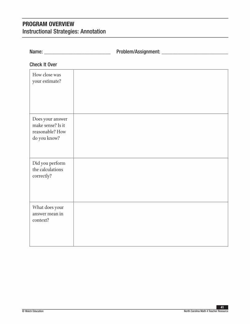
© Walch Education41
North Carolina Math 4 Teacher Resource
PROGRAM OVERVIEWInstructional Strategies: Annotation
Name: _________________________ Problem/Assignment: _________________________
Check It Over
How close was your estimate?
Does your answer make sense? Is it reasonable? How do you know?
Did you perform the calculations correctly?
What does your answer mean in context?

42© Walch EducationNorth Carolina Math 4 Teacher Resource
PROGRAM OVERVIEWInstructional Strategies: Annotation
Annotation Strategies CUBES Protocol
What is the annotation strategy CUBES?
CUBES is an annotation strategy in which students use different written designs to highlight the key aspects of word problems. It can help them choose the correct mathematical strategy to solve the problem accurately.
How do you implement CUBES in the classroom?
The steps for CUBES are:
1. C: Circle all the key numbers.
2. U: Underline the question.
3. B: Box in the key words that will determine the operation(s) necessary and write the mathematical symbol for the operation(s).
4. E: Evaluate the information given to determine the strategy needed. Eliminate any unnecessary information.
5. S: Solve the problem, show your work, and check your answer.
As students learn to use CUBES, walk them through the steps individually to ensure they can accurately identify the key numbers, question, key words, unnecessary information, and strategy. Work through each step individually for several “easy” problems first, so that difficult math doesn’t interfere with the process. Increase the problem difficulty incrementally as students begin to master the process. This may seem like a long process at first, but the ultimate result is worth the time investment.
A graphic organizer can help students master the process, especially when problems are given on a computer or tablet where students can’t always annotate directly on the problem. Students can write down the key numbers and circle them, write down the question and underline it, and so on. This will encourage students to truly think about the different pieces of the problem they are identifying, and how these pieces will guide the strategy and affect the solution.
When would I use CUBES in the classroom?
CUBES can be used to solve any math problem, and is especially helpful for word problems. When CUBES is initially implemented, the steps should be discussed in detail. As students become accustomed to using CUBES and begin thinking about problems in this manner automatically, the individual steps become less important and can be scaffolded out to improve efficiency. However, the teacher should ensure that students are truly evaluating all the key information before routine discussions of the individual steps are removed.

© Walch Education43
North Carolina Math 4 Teacher Resource
PROGRAM OVERVIEWInstructional Strategies: Annotation
How can I use CUBES with students needing additional support?
Design features can help students identify key words and features, even when certain vocabulary words are not known. As teachers introduce the content-specific Tier 3 vocabulary to their classes, annotation strategies such as CUBES can help students use these words to apply appropriate strategies while problem solving. Using circles, underlines, and boxes can help students organize the key facts and vocabulary, and the elimination of unnecessary information can simplify the problem. This strategy is especially beneficial for ESL students.
Combining CUBES with graphic organizers also benefits ESL students by removing a lot of the confusing wording and allowing them to focus on the important facts of a problem. When using CUBES with a graphic organizer, all students, including ESL students, will begin to think about problem solving in a way that helps encourage them to use the appropriate information to find a solution.
What other standards does the CUBES Protocol address?
Standards of Mathematical Practice:
• SMP.1
• SMP.2
• SMP.5
• SMP.6
WIDA English Language Development Standards:
• ELD Standard 3
Language Arts Standards:
• ELA–LITERACY.WHST.9–10.4
• ELA–LITERACY.SL.9–10.4
• ELA–LITERACY.SL.9–10.3
• ELA–LITERACY.SL.9–10.2
• ELA–LITERACY.RST.9–10.4
Source
• Margaret Tibbett. “Comparing the effectiveness of two verbal problem solving strategies: Solve It! and CUBES.”
https://rdw.rowan.edu/cgi/viewcontent.cgi?article=2633&context=etd

44© Walch EducationNorth Carolina Math 4 Teacher Resource
PROGRAM OVERVIEWInstructional Strategies: Graphic Organizers
Organizing Mathematical Content: Graphic Organizers Organizing mathematical content is a crucial skill for problem solving, exploring other possible methods for finding solutions, and managing math content. All students need strategies for organizing content to build conceptual understanding. For students with disabilities, visual representations and graphic organizers can help them clarify their thoughts and focus on the math. ESL students also benefit from visual representations and graphic organizers. Organizing mathematical knowledge with visuals can help ESL students navigate math content while learning the language. Graphic organizers include Frayer Models and Tables of Values.
LiteracyStrategies
MathematicalDiscourseStrategies
AnnotationStrategies
GraphicOrganizerStrategies

© Walch Education45
North Carolina Math 4 Teacher Resource
PROGRAM OVERVIEWInstructional Strategies: Graphic Organizers
Graphic Organizers Frayer Models
What is a Frayer Model?
A Frayer Model is a graphic organizer that can help students understand new vocabulary words and concepts by exploring their characteristics. A Frayer model lists the definition of a word or concept, describes some key facts, and gives examples and non-examples. Examples and non-examples can come from a mathematical or real-world context.
How do you implement Frayer Models in the classroom?
Students can learn to create Frayer Models the first week of school, and the process can be used throughout the year each time students experience a new word or concept.
While it is important for teachers to give students precise mathematical definitions with appropriate content vocabulary, it is maybe more important for students to understand the application of mathematical words and concepts in their own context. As students learn new information, small group discussions and think-pair-share activities are great ways for students to formulate their own definitions, review the characteristics and facts they have learned, and discuss examples and non-examples.
Discussions of the examples and non-examples can help lead to the mathematical definition. For example, if students use a Frayer Model to define a quadratic function, they would notice that all examples have a highest exponent of 2, and all non-examples would not have a highest exponent of 2. All examples would have parabolic graphs, and all non-examples would have other graphs. Through these comparisons, students will understand the definition of quadratics using different representations, and they will be able to apply it in different contexts.
When would I use Frayer Models in the classroom?
Frayer Models can be used at different points during instruction. They are appropriate as introductions to new concepts, summaries to ensure understanding of new concepts, or as note-organizers throughout the lesson for students to fill in as they learn new concepts. At first, students might need help figuring out how to list and differentiate between the definition, facts and characteristics, examples, and non-examples. As students adapt to the process, they will be able to categorize information on their own or in small groups. As they compare newer Frayer Models to previous models, they will also be able to see how concepts build upon each other.

46© Walch EducationNorth Carolina Math 4 Teacher Resource
PROGRAM OVERVIEWInstructional Strategies: Graphic Organizers
How can I use Frayer Models with students needing additional support?
Frayer Models can be a point of reference for students as they progress throughout the year. As students determine their own definitions for math-specific words and concepts, and use the examples and non-examples to determine the key facts, they will be able to put them in their own context and apply them to solve complicated problems. As math concepts build upon each other both within a unit and throughout the year, the use of Frayer Models to remind students of their initial definitions of words or concepts can help solidify their understanding. Using Frayer Models as part of a Word Wall or Concept Wall, or having a consistent notebook process to reference past Frayer models, can help consistently reinforce learning.
What other standards do Frayer Models address?
Standards of Mathematical Practice:
• SMP.1
• SMP.2
• SMP.6
WIDA English Language Development Standards:
• ELD Standard 3
Language Arts Standards:
• ELA–LITERACY.WHST.9–10.4
• ELA–LITERACY.WHST.9–10.1
• ELA–LITERACY.SL.9–10.1
• ELA–LITERACY.SL.9–10.4
• ELA–LITERACY.RST.9–10.3
• ELA–LITERACY.RST.9–10.4
Source
• Deborah K. Reed. “Building Vocabulary and Conceptual Knowledge Using the Frayer Model.”
https://iris.peabody.vanderbilt.edu/module/sec-rdng/cresource/q2/p07/
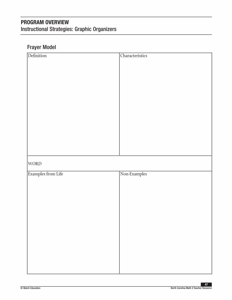
© Walch Education47
North Carolina Math 4 Teacher Resource
PROGRAM OVERVIEWInstructional Strategies: Graphic Organizers
Frayer ModelDefinition Characteristics
WORD
Examples from Life Non-Examples

48© Walch EducationNorth Carolina Math 4 Teacher Resource
PROGRAM OVERVIEWInstructional Strategies: Graphic Organizers
Graphic OrganizersTables of Values
What is a Table of Values?
A Table of Values is an organized way to list numbers that represent different categories of values. These values can be represented as ordered pairs, graphs, word problems, or lists. Tables can help students see and compare values in a different way.
How do you implement Tables of Values in the classroom?
Tables can be used throughout the year to support various mathematical standards. Some standards mention tables specifically, and in others, tables can be an effective support to help students organize and understand the meaning and application of values.
Tables can be set up with numerical values in rows or columns. The key to understanding the values lies in the headings. The headings must be specific enough to show students the meaning and/or application of the numerical values, but not so wordy that they interfere with the clarity of the numbers in the table. For example:
x (year)y (population in millions)
1960 219
1970 230
1980 258
1990 312
2000 342
Mean (statistical average) 50 45
Median (middle value) 52 43
Quartile 1 (median of the lower 50%) 40 38
Quartile 3 (median of the upper 50%) 72 80
Range (difference of max and min values) 80 61
Interquartile Range (difference of quartiles) 32 42
Standard Deviation (measure of spread of data) 7.24 10.23
© Walch Education49
North Carolina Math 4 Teacher Resource
PROGRAM OVERVIEWInstructional Strategies: Graphic Organizers
When would I use Tables of Values in the classroom?
Various mathematical topics can be represented by tables. For example:
• An (x, y) table of values to represent coordinates on a graph or independent and dependent variables for a given context
• A table to represent coefficients and/or constants in an equation
• A table to show different statistical measures when comparing sets of data
• A table to compare output values for the same input given different functions
Each time numbers or values are being listed, compared, or graphed, a table can help students differentiate between the values. Tables are easy to create, and students can be encouraged to create them as another representation to clarify and compare numbers for nearly any topic.
How can I use Tables of Values with students needing additional support?
Tables of Values can help students focus on numerical values and their meaning in context without distraction. They clarify what each number represents, what numbers can be compared, and what ordered pairs can be graphed to give a visual representation. Additionally, headings can be used to either highlight the relevant facts from a context or to describe mathematical vocabulary.
In general, graphic organizers benefit students by removing much of the confusing wording and focusing on the important facts and numbers of a problem.
What other standards do Tables of Values address?
Standards of Mathematical Practice:
• SMP.1
• SMP.2
• SMP.6
WIDA English Language Development Standards:
• ELD Standard 3
Language Arts Standards:
• ELA–LITERACY.WHST.9–10.4
• ELA–LITERACY.WHST.9–10.1
• ELA–LITERACY.SL.9–10.1
• ELA–LITERACY.SL.9–10.4
• ELA–LITERACY.RST.9–10.3
• ELA–LITERACY.RST.9–10.4
Source • Alliance for Excellent Education. “Six Key Strategies for Teachers of English Language Learners.”
https://uteach.utexas.edu/sites/default/files/files/SixKeyStrategiesELL.pdf

50© Walch EducationNorth Carolina Math 4 Teacher Resource
PROGRAM OVERVIEWInstructional Strategies: Mathematical Discourse
Communicating Mathematical Content: Mathematical Discourse Reading, writing, speaking, and listening are all important ways to learn and express information, but the last two ways are often slighted in the math classroom. The mathematical discourse strategies presented here promote speaking and listening in a math-focused literacy context. Working these strategies into the daily routine of a classroom can help students become comfortable speaking and listening in a mathematical context, which will help them become comfortable with the mathematical content. Routines and structures are essential to support students with disabilities, as they often benefit from following a routine. This can lead to developing capability in their mathematical skills. These strategies also remove the barrier to entry for many ESL students, as structure and routine can help them focus on the math content rather than English language deficiencies. Mathematical Discourse strategies include Sentence Starters and Small Group Discussion.
LiteracyStrategies
MathematicalDiscourseStrategies
AnnotationStrategies
GraphicOrganizerStrategies

© Walch Education51
North Carolina Math 4 Teacher Resource
PROGRAM OVERVIEWInstructional Strategies: Mathematical Discourse
Mathematical Discourse StrategiesSentence Starters
What is a Sentence Starter?
A Sentence Starter is a common phrase or mathematical sentence frame that can help students begin and sustain academic conversations around mathematical content. It helps guide students through the discussion and bring out pertinent ideas that can lead to greater understanding.
How do you implement Sentence Starters in the classroom?
Many people view math class as a place to calculate solutions to math problems. However, to ensure the conceptual understanding and proper application of a math concept, students need to be able to explain the concepts and reasoning behind a solution to a problem. As many students are not accustomed to having academic conversations about math, sentence starters can help begin and continue these conversations in a productive manner.
There are two main types of sentence starters for mathematical discussions: discourse starters and math starters. For example, a poster with these or other sentence starters can be displayed from the beginning of the year, and the expectation can be set that any answer to a question or comment in a discussion should be framed using one of these starters. As students become accustomed to framing mathematical conversations in this way, they can expand on the given sentence starters and create some of their own. They will begin to realize how these statements ensure that their conversations revolve around math, enhance understanding of the concept, and force them not only to state, but also to explain their thinking. They will gain confidence from the ability to engage, as the first step has already been taken for them.
When would I use Sentence Starters in the classroom?
Sentence Starters can be used throughout the entire school year with any concept. However, they are most important to use at the beginning of the school year to build a mathematical community in the classroom centered on a comfort with mathematical discourse. Especially at the beginning of the year, students should be encouraged to use these sentence starters for every math statement. Appropriate settings include during small group discussion, while responding to whole class questions, and when writing explanations for problem solutions.
Modifications can be introduced so that students must use certain mathematical vocabulary within the sentences, or must use certain sentence starters at different points in conversations or for different conversation types and situations. However the starters are implemented, it is important for students to realize that these are intended to enhance and focus their conversations, not limit them.

52© Walch EducationNorth Carolina Math 4 Teacher Resource
PROGRAM OVERVIEWInstructional Strategies: Mathematical Discourse
How can I use Sentence Starters with students needing additional support?
Often, students are reluctant to talk about math concepts because they either lack confidence in their knowledge, are afraid to be “wrong,” or don’t know how to start or continue the conversation. Sentence starters can help students overcome this reluctance. The non-threatening, easy-to-interpret sentence starters remove the barrier to entry for students who don’t know how to engage, and the respectful, mathematical focus promoted by sentence starters can help build confidence and provide a structure so that students will not fear being wrong.
For ESL students specifically, sentence starters can provide the English language support to help students engage with and discuss the math. The support of sentence structure removes language barriers to entry for students who don’t fully understand English sentence structure.
Discourse Starters Math StartersI agree/disagree with … because …
I understand/don’t understand …
First/Next/Finally I … because …
I noticed that …
I wonder …
My answer was … because …
The next step is … because …
I used (insert formula/equation/concept) because …
My answer is right/reasonable because …
What other standards do Sentence Starters address?
WIDA English Language Development Standards
• ELD Standard 3
Standards of Mathematical Practice:
• SMP.1
• SMP.3
• SMP.6
Language Arts Standards:
• ELA–LITERACY.WHST.9–10.4
• ELA–LITERACY.WHST.9–10.1
• ELA–LITERACY.SL.9–10.1
• ELA–LITERACY.SL.9–10.4
• ELA–LITERACY.RST.9–10.3
• ELA–LITERACY.RST.9–10.4
Source
• AVID. “Sentence Starters.”
https://sweetwaterschools.instructure.com/files/29100523/download?download_frd=1&verifier=CBvje9CPNKUe6IkN4TPBJDuXmZY3464aTTK1Fk2r math sentence starters research
© Walch Education53
North Carolina Math 4 Teacher Resource
PROGRAM OVERVIEWInstructional Strategies: Mathematical Discourse
Mathematical Discourse StrategiesSmall Group Discussion
What is Small Group Discussion?
Small Group Discussion is a structured way for students to verbalize their mathematical thinking in a comfortable setting to solve a problem, build conceptual understanding, or summarize a concept.
How do you implement Small Group Discussion?
Small Group Discussion in math class depends on a trusting relationship between the teacher and the students. From there, students can build trusting relationships among themselves. Once this trust has been built, students will feel free to explore mathematical topics in groups, take risks, and engage in a productive struggle toward understanding or a solution.
Once these relationships have been established, certain structures should be established for Small Group Discussion to be effective. Discussion norms can be set by the class to ensure discussions are respectful and productive, and discussions should have predetermined time limits. The group composition is also important and should be based on instructional measures. For different activities, homogeneous groups, heterogeneous groups, or groups based on specific data by standard could be appropriate. Students should always be aware that the groups were chosen to maximize their learning.
Another structure that can be effective for Small Group Discussion is assigning group roles. These roles can include group leader, note taker, timekeeper, resource manager, culture keeper, or other roles determined to be appropriate for the classroom context. During the discussion, assigning each student a letter within the group (A, B, C, D, etc.) can help structure the discussion. Different roles can specify certain time limits for talk, which sentence starters to use, or other structured aspects of the discussion.
When implementing a Small Group Discussion, the question or task should inspire students to think in different ways about a concept. Through the structured format of the discussion, students will compare their ideas and arrive at an answer or explanation of the concept. Within the trusting framework of the class and group, students can focus on the common goal of the discussion and develop their thinking around the math concept. These rich discussions will enhance their understanding.
When would I use Small Group Discussion in the classroom?
Small Group Discussion can be used for nearly any topic, and it can be used at a variety of times in the classroom. The questions and tasks may need to change depending on when it is used. Opening activities for lessons can be Small Group Discussions where students explore properties of new math concepts or review/build upon their prior learning. Turn and talks throughout the lesson can be structured as Small Group Discussions if a consistent framework is in place. At the end of class, a Small Group Discussion can be used to come to a common understanding about an essential question from the lesson.

54© Walch EducationNorth Carolina Math 4 Teacher Resource
PROGRAM OVERVIEWInstructional Strategies: Mathematical Discourse
Depending on when the Small Group Discussion is used in class, and what the goal of the discussion is, the discussion reporting may vary. For a warm-up, each group might be asked to share their thinking. For a guided practice, recording answers on chart paper and a gallery walk could be appropriate. For a closing activity, individual written responses to a question could be appropriate.
How can I use Small Group Discussion with students needing additional support?
As discussed in other Mathematical Discourse strategies, struggling students are reluctant to talk about math concepts because they lack confidence in their knowledge and don’t always have the needed vocabulary in their toolbox. Structured discussions with effective grouping can help students through these barriers. After a trusting and respectful classroom environment has been established, struggling students often feel more comfortable sharing their ideas with just a few classmates rather than the whole class. Additionally, adding structure can help students engage by providing the expectation that they participate in the process.
The intentional grouping of students can also help them succeed using Small Group Discussion. At times, heterogeneous groups could be appropriate so that stronger students can help struggling students, and at other times, homogeneous groups could be appropriate so the teacher can work with an entire group of struggling students. ESL students can be grouped with other students with the same dominant language to help remove the language barrier from the conversation.
What other standards does Small Group Discussion address? WIDA English Language Development Standards:
• ELD Standard 3
Standards of Mathematical Practice:
• SMP.1
• SMP.3
• SMP.6
Language Arts Standards:
• ELA–LITERACY.WHST.9–10.4
• ELA–LITERACY.WHST.9–10.1
• ELA–LITERACY.SL.9–10.1
• ELA–LITERACY.SL.9–10.4
• ELA–LITERACY.RST.9–10.3
• ELA–LITERACY.RST.9–10.4
Source
• Jessie C. Store. “Developing Mathematical Practices: Small Group Discussions.”
https://kb.osu.edu/dspace/bitstream/handle/1811/78055/OJSM_69_Spring2014_12.pdf
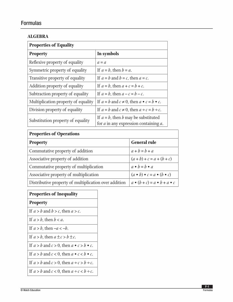
Formulas
Properties of Equality
Property In symbols
Reflexive property of equality a = a
Symmetric property of equality If a = b, then b = a.
Transitive property of equality If a = b and b = c, then a = c.
Addition property of equality If a = b, then a + c = b + c.
Subtraction property of equality If a = b, then a – c = b – c.
Multiplication property of equality If a = b and c ≠ 0, then a • c = b • c.
Division property of equality If a = b and c ≠ 0, then a ÷ c = b ÷ c.
Substitution property of equalityIf a = b, then b may be substituted for a in any expression containing a.
Properties of Operations
Property General rule
Commutative property of addition a + b = b + a
Associative property of addition (a + b) + c = a + (b + c)
Commutative property of multiplication a • b = b • a
Associative property of multiplication (a • b) • c = a • (b • c)
Distributive property of multiplication over addition a • (b + c) = a • b + a • c
Properties of Inequality
Property
If a > b and b > c, then a > c.
If a > b, then b < a.
If a > b, then –a < –b.
If a > b, then a ± c > b ± c.
If a > b and c > 0, then a • c > b • c.
If a > b and c < 0, then a • c < b • c.
If a > b and c > 0, then a ÷ c > b ÷ c.
If a > b and c < 0, then a ÷ c < b ÷ c.
ALGEBRA
Formulas© Walch EducationF-1

Formulas
Symbols
≈ Approximately equal to
≠ Is not equal to
a Absolute value of a
a Square root of a
∞ Infinity
[ Inclusive on the lower bound
] Inclusive on the upper bound
( Non-inclusive on the lower bound
) Non-inclusive on the upper bound
∑ Sigma
∆ Delta
Linear Equations
2 1
2 1
my y
x x=
−− Slope
y = mx + b Slope-intercept form
ax + by = c General form
y – y1 = m(x – x1) Point-slope form
Exponential Equations
= +
A Pr
n
nt
1 Compounded interest formula
A = PertContinuously compounded interest formula
Compounded…n (number of times per year)
Yearly/annually 1
Semiannually 2
Quarterly 4
Monthly 12
Weekly 52
Daily 365
Coordinates
(x, y) Ordered pair
(x, 0) x-intercept
(0, y) y-intercept
Exponential Functions
1 + r Growth factor
1 – r Decay factor
= +f t a r t( ) (1 ) Exponential growth function
= −f t a r t( ) (1 ) Exponential decay function
=f x abx( ) Exponential function in general form
Binomial Theorem
!
! !• 1
1
( 1)
1•2
( 1)( 2)
1•2•31
0
0 1 1 2 2 3 3 0
n
n k ka b a b
na b
n na b
n n na b a bn k k
k
nn n n n n∑( )−
= + +−
+− −
+ +−
=
− − −
Formulas © Walch EducationF-2

Formulas
Functions
f(x) Function notation, “f of x”
f –1(x) Inverse function notation
f(x) = mx + b Linear function
f(x) = b x + k Exponential function
f(x) = ax 2 + b x + c Quadratic function
(f + g)(x) = f(x) + g(x) Addition
(f – g)(x) = f(x) – g(x) Subtraction
(f • g)(x) = f(x) • g(x) Multiplication
=f
gx
f x
g x( )
( )
( )Division
( )( ) ( ( ))f g x f g x= Composition
−−
f b f a
b a
( ) ( )Average rate of change
rf x
g x
�
�
( )
( )= Concise rate of change
f(–x) = –f(x) Odd function
f(–x) = f(x) Even function
= f x x( ) Floor/greatest integer function
= f x x( ) Ceiling/least integer function
– 1– 1
22
1 0f x a x a x a x a x ann
nn( ) = + + + + + Polynomial function
= − +f x a x h k( ) ( )3 Cube root function
( ) ( )f x a x h kn= − + Radical function
= − +f x a x h k( ) Absolute value function
= ≠f xp x
q xq x( )
( )
( ); ( ) 0 Rational function
y = logax Logarithmic function
Formulas© Walch EducationF-3

Formulas
Common Polynomial Identities
(a + b)2 = a2 + 2ab + b2 Square of Sums
(a – b)2 = a2 – 2ab + b2 Square of Differences
a2 – b2 = (a + b)(a – b) Difference of Two Squares
a3 + b3 = (a + b)(a2 – ab + b2) Sum of Two Cubes
a3 – b3 = (a – b)(a2 + ab + b2) Difference of Two Cubes
Quadratic Functions and Equations
=−
xb
a2 Axis of symmetry
=+
xp q
2
Axis of symmetry using the midpoint of the x-intercepts
− −
b
af
b
a2,
2 Vertex
f(x) = ax2 + bx + c General form
f(x) = a(x – h)2 + k Vertex form
f(x) = a(x – p)(x – q) Factored/intercept form
b2 – 4ac Discriminant
+ +
x bxb
22
2
Perfect square trinomial
=− ± −
xb b ac
a
4
2
2
Quadratic formula
Properties of Exponents
Property General rule
Zero Exponent a0 = 1
Negative Exponent1
=−aa
nn
Product of Powers • = +a a am n m n
Quotient of Powers = −a
aa
m
nm n
Power of a Power ( ) =b bm n mn
Power of a Product ( ) =bc b cn n n
Power of a Quotient
=a
b
a
b
m m
m
Properties of Radicals
•=ab a b
=a
b
a
b
Radicals to Rational Exponents
=a an n
1
=x xmnm
n
Logarithmic Functions
e Base of a natural logarithm
loglog
logb
b
aa = Change of base formula
Properties of Logarithms
Product property loga (x • y) = loga x + logb y
Quotient property log log logx
yx ya a a
= −
Power property loga xy = y • loga x
Formulas © Walch EducationF-4

Formulas
Imaginary and Complex Numbers
a + bi Standard form of a complex number
a – bi Conjugate of a + bi
a2 + b2 Product of conjugates a + bi and a – bi
2 2+a b Modulus of a complex number, +a bi
1= −i Definition of the imaginary number i
i2 = –1 Definition of i squared
i3 = –i Definition of i cubed
i4 = 1 Definition of the fourth power of i
Sequences and Series
d = an – an – 1 Common difference
an = a1 + (n – 1)d Explicit formula for an arithmetic sequence
an = an – 1 + d Recursive formula for an arithmetic sequence
1
ra
an
n
=−
Common ratio
an = a1 • rn – 1 Explicit formula for a geometric sequence
an = an – 1 • r Recursive formula for a geometric sequence
11
1
a r k
k
n
∑ −
=Finite geometric series
11
1
a r k
k∑ −
=
∞
Infinite geometric series
(1 )
11S
a r
rn
n
=−−
Sum formula for a finite geometric series
11S
a
rn = −Sum formula for an infinite geometric series
1
11
1
P Aik
n k
∑= +
=
−
Amortization loan formula
Formulas© Walch EducationF-5

Formulas
STATISTICS AND DATA ANALYSIS
Symbols
∅ Empty/null set
∩ Intersection, “and”∪ Union, “or” Subset
A Complement of Set A
! FactorialCn r CombinationPn r Permutation
IQR Interquartile rangeµ Population mean
x Sample meanMAD Mean absolute deviationσ Standard deviation of a populations Standard deviation of a sampleσ 2 Variancep̂ Sample proportion
SEM Standard error of the meanSEP Standard error of the proportionMOE Margin of errorCI Confidence intervaldf Degrees of freedom
Common Critical Values
Confidence level 99% 98% 96% 95% 90% 80% 50%
Critical value (zc) 2.58 2.33 2.05 1.96 1.645 1.28 0.6745
Empirical Rule/68–95–99.7 Rule1 68%± ≈� �
2 95%± ≈� �
3 99.7%± ≈� �
Formulas © Walch EducationF-6

Formulas
Formulas
IQR = Q 3 – Q 1 Interquartile range
Q 1 – 1.5(IQR) Lower outlier formula
Q 3 + 1.5(IQR) Upper outlier formula
y – y0 Residual formula
1 2 x x x
nnµ =
+ + +Mean of a population
1 2
xx x x
nn=
+ + +Mean of a sample
x x
niMAD=
∑ −Mean absolute deviation
( )2
1
x
n
ii
n
∑=
−=�
�Standard deviation of a population
sx x
n
ii
n2
1∑( )
=−
= Standard deviation of a sample
x x
ni2
2
σ( )
=∑ −
Variance
zx
=−�
�z-score
p̂p
n= Sample proportion
SEMs
n= Standard error of the mean
SEPˆ 1 ˆp p
n
( )=
−Standard error of the proportion
MOE zs
nc= ± Margin of error of a sample mean
MOEˆ 1 ˆ
zp p
nc
( )= ±
−Margin of error for a sample proportion
CI ˆˆ 1 ˆ
p zp p
nc
( )= ±
− Confidence interval for a sample population with proportion p̂
Formulas© Walch EducationF-7

Formulas
Rules and Equations
=P EE
( )# of outcomes in
# of outcomes in sample space Probability of event E
∪ = + − ∩P A B P A P B P A B( ) ( ) ( ) ( ) Addition rule
= −P A P A( ) 1 ( ) Complement rule
( )= ∩P B A
P A B
P A
( )
( ) Conditional probability
E(X) = X1 • P(X1) + X2 • P(X2) + X3 • P(X3) + … + Xn • P(Xn) Expected value
( ) ( )• ( )∩ =P A B P A P B A Multiplication rule
( ) ( )• ( )∩ =P A B P A P B Multiplication rule if A and B are independent
=−
Cn
n r rn r
!
( )! ! Combination
=−
Pn
n rn r
!
( )!Permutation
n n n n! •( 1)•( 2) • • 1= − − Factorial
P nx
p qx n x=
−Binomial probability distribution
Formulas, continued
CI x zs
nc= ± Confidence interval for a sample population with mean x
1 2
12
1
22
2
=−
+
tx x
s
n
s
nt-value for two sets of sample data
0µ=−
tx
s
nt-value for sample data and population
1 1
21 2=− + −
dfn n
Degrees of freedom
Formulas © Walch EducationF-8

Formulas
TRIGONOMETRY
Unit Circle
( , )
( , )
( , )
( ,
)
(
,
)(
,
)
( , )( , )( , )
60°
45°
30°
120°135°
180° 0°
150°
90°
270°
210°
225°
240°
330°
300°
315°
3π2
5π3
7π4
611π
65π
3π4
2π3
π2
6
4
3π
π
π
34π
45π67π
π
22
13
3
( ,
)
( ,
)
( ,
)
22 1
–
–2
2
22
31–
2
2
32
21 2
22
2
22
31
22
3
1
2
2
2
2
–
––
–
–
–
1
2
23
3
22 1
–
––
2
22
2
y
x
(0, 1)
(1, 0)(–1, 0)
(0, –1)
0360° 2π
Trigonometric Ratios
θ =sinopposite
hypotenuseθ =cos
adjacent
hypotenuseθ =tan
opposite
adjacent
θ =cschypotenuse
oppositeθ =sec
hypotenuse
adjacentθ =cot
adjacent
opposite
Inverse Trigonometric Functions
Arcsin θ = sin–1θ
Arccos θ = cos–1θ
Arctan θ = tan–1θ
Laws of Sines and Cosines
sin sin sin= =
a
A
b
B
c
CLaw of Sines
c2 = a2 + b2 – 2ab cos C Law of Cosines
Converting Between Degrees and Radians
π=
radian measure degree measure
180
Formulas© Walch EducationF-9

Formulas
Common Trigonometric Identities
Even-odd identities cos (–θ) = cos θ sin (–θ) = –sin θ tan (–θ) = –tan θ sec (–θ) = sec θ csc (–θ) = –csc θ cot (–θ) = –cot θ
Pythagorean identitiessin2 θ + cos2 θ = 1 1 + tan2 θ = sec2 θ 1 + cot2 θ = csc2 θ
Ratio identities tansin
cosθ
θθ
= cotcos
sinθ
θθ
=
Reciprocal identities sin
1
cscθ
θ= cos
1
secθ
θ= tan
1
cotθ
θ=
csc1
sinθ
θ=
sec
1
cosθ
θ=
cot
1
tanθ
θ=
Angle Sum and Difference Identities
sin (α + β) = sin α cos β + cos α sin β sin (α – β) = sin α cos β – cos α sin β
cos (α + β) = cos α cos β – sin α sin β cos (α – β) = cos α cos β + sin α sin β
α βα β
α β( )+ =
+−
tantan tan
1 tan tantan
tan tan
1 tan tanα β
α βα β
( )− =−
+
Double-Angle Identitiescos 2θ = 1 – 2 sin2 θ sin 2θ = 2 cos θ sin θ
cos 2θ = cos2 θ – sin2 θ θθθ
=−
tan22tan
1 tan2
cos 2θ = 2 cos2 θ – 1
Half-Angle Identities
tan2
1 cos
1 cos
θ θθ
= ±
−+
θ θ
= ±
−sin
2
1 cos
2
tan2
1 cos
sin
θ θθ
=
− θ θ
= ±
+cos
2
1 cos
2
tan2
sin
1 cos
θ θθ
=
+
Formulas © Walch EducationF-10

Formulas
Transformations of Trigonometric Functions
a Amplitude2πb
Period
−b
aPhase shift
d Vertical shift
Function Domain Range
sin xπ π
−
2
,2
[–1, 1]
sin–1 x [–1, 1]π π
−
2
,2
cos x [0, π] [–1, 1]cos–1 x [–1, 1] [0, π]
tan xπ π
−
2
,2
(–∞, ∞)
tan–1 x (–∞, ∞)π π
−
2
,2
Formulas© Walch EducationF-11

Formulas
MATRICES
+
=
++
ab
cd
a cb d
Addition of matrices
−
=
−−
ab
cd
a cb d
Subtraction of matrices
••
•
=
a bc
a b
a cMultiplication of a matrix by a scalar
•• • • •
• • • •
=
+ ++ +
a bc d
w xy z
a w b y a x b z
c w d y c x d zMultiplication of matrices
det A = ad – bc The determinant of =
A a b
c d.
1
det•1 = −
−
−AA
d bc a
The inverse of =
A a b
c d.
•
=
a bm n
xy
cp
The system of equations + =+ =
ax by c
mx ny p
written as a matrix equation
1 00 1
Multiplicative identity matrix for 2 × 2 matrix
1 0 00 1 00 0 1
Multiplicative identity matrix for 3 × 3 matrix
Formulas © Walch EducationF-12

Formulas
TRANSFORMATION MATRICES
Matrix Translation
1
1
2
2
3
3
+
x
y
x
y
x
y
p
q
p
q
p
q
Translation of A(x1, y1), B(x2, y2), C(x3, y3) to the right by p units and up by q units
Matrix Angle of rotation
−
0 11 0
90°
−−
1 00 1
180°
−
0 11 0
270°
Matrix Line of reflection
−
1 00 1
y-axis
−
1 00 1
x-axis
0 11 0
line y = x
Formulas© Walch EducationF-13

Formulas
VECTORS
2 2= +a bvMagnitude of vector
,=v a b with initial point at the origin
( ) ( )2 12
2 12= = − + −x x y yv PQ
Magnitude of vector � � ��
=v PQ with P(x1, y1) and Q(x2, y2)
,+ = + +u v a c b dAddition of vectors
,=u a b and
,=v c d
• , • , •=c a b c a c b Scalar multiplication of a vector
v
vUnit vector of
v
Formulas © Walch EducationF-14
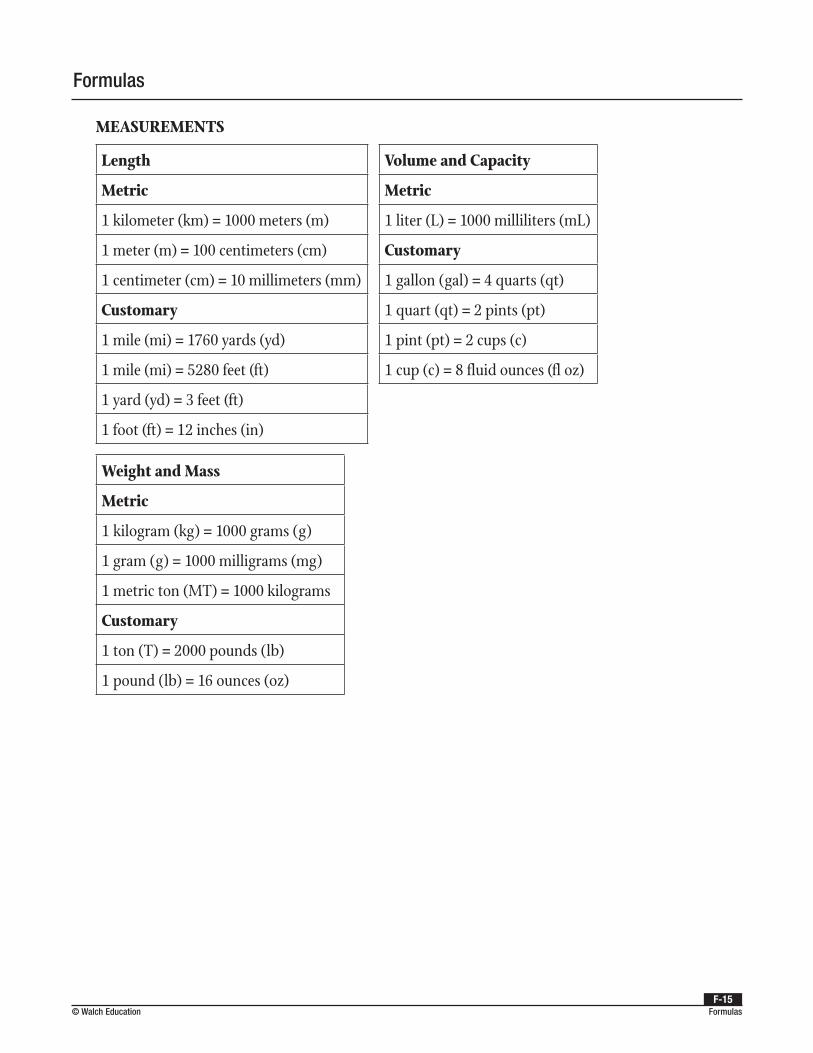
Formulas
MEASUREMENTS
Length
Metric
1 kilometer (km) = 1000 meters (m)
1 meter (m) = 100 centimeters (cm)
1 centimeter (cm) = 10 millimeters (mm)
Customary
1 mile (mi) = 1760 yards (yd)
1 mile (mi) = 5280 feet (ft)
1 yard (yd) = 3 feet (ft)
1 foot (ft) = 12 inches (in)
Volume and Capacity
Metric
1 liter (L) = 1000 milliliters (mL)
Customary
1 gallon (gal) = 4 quarts (qt)
1 quart (qt) = 2 pints (pt)
1 pint (pt) = 2 cups (c)
1 cup (c) = 8 fluid ounces (fl oz)
Weight and Mass
Metric
1 kilogram (kg) = 1000 grams (g)
1 gram (g) = 1000 milligrams (mg)
1 metric ton (MT) = 1000 kilograms
Customary
1 ton (T) = 2000 pounds (lb)
1 pound (lb) = 16 ounces (oz)
Formulas© Walch EducationF-15


Glossary
English Unit/Lesson Español
#
68–95–99.7 rule a rule that states percentages of data under the normal curve are as follows: 1 68%µ σ± ≈ ,
2 95%µ σ± ≈ , and 3 99.7%µ σ± ≈ ; also known as the Empirical Rule
6.3 regla 68–95–99,7 regla que establece los siguientes porcentajes de datos bajo la curva normal: 1 68%µ σ± ≈ ,
2 95%µ σ± ≈ y 3 99.7%µ σ± ≈ , ; también se la conoce como Regla Empírica
A
absolute value a number’s distance from 0 on a number line; the positive value of a quantity
8.6 valor absoluto distancia de un número a partir del 0 en una recta numérica; valor positivo de una cantidad
absolute value function a function with a variable inside an absolute value
2.1 función de valor absoluto función con una variable dentro de un valor absoluto
addition rule for mutually exclusive events If events A and B are mutually exclusive, then the probability that A or B will occur is the sum of the probability of each event; P(A or B) = P(A) + P(B).
6.7 6.8
regla de adición para eventos mutuamente excluyentes Si los eventos A y B son mutuamente excluyentes, la probabilidad de que A o B suceda es la suma de la probabilidad de cada evento; P(A or B) = P(A) + P(B).
additive identity the element of a set whose addition does not change other elements; the additive identity of the real numbers is 0
8.7 identidad de la suma es el elemento de un conjunto cuya sumatoria no cambia a los demás elementos; la identidad de la suma en los números reales es el 0
additive identity matrix a matrix for which all entries are 0; the matrix whose addition does not change other matrices; also known as the zero matrix
8.7 matriz identidad de la suma matriz cuyas entradas son todas 0; es la matriz cuya sumatoria no cambia a las demás matrices; también se la conoce como la matriz cero
additive inverse matrix the matrix which, when added to matrix A, yields the zero matrix; also called the opposite matrix. The additive inverse of A is –A.
8.7 matriz inversa aditiva es la matriz que, cuando se la suma a una matriz A, el resultado es la matriz cero; también se la llama matriz opuesta. La inversa aditiva de A es –A.
altitude the perpendicular line from a vertex of a figure to its opposite side; height
4.2 altitud línea perpendicular desde el vértice de una figura hasta su lado opuesto; altura
North Carolina Math 4 Teacher Resource
© Walch EducationG-1

Glossary
English Unit/Lesson Español
ambiguous case a situation wherein the Law of Sines produces two possible answers. This only occurs when the lengths of two sides and the measure of the non-included angle are given (SSA).
4.2 caso ambiguo situación en la cual la Ley de Senos produce dos respuestas posibles. Esto solo ocurre cuando están dadas las longitudes de los dos lados y la medida del ángulo no incluido (SSA).
amplitude the coefficient a or c of the sine or cosine term in a function of the form f(x) = a sin bx or g(x) = c cos dx; on a graph of the cosine or sine function, the vertical distance from the y-coordinate of the maximum point on the graph to the midline of the cosine or sine curve
4.5 amplitud el coeficiente a o c del término de seno o coseno en una función de la forma f(x) = a sin bx o g(x) = c cos dx; en un gráfico de la función seno o coseno, la distancia vertical desde la coordenada y del punto máximo en la gráfica hasta la línea media de la curva de seno o coseno
arccosine the inverse of the cosine function, written cos–1 θ or arccos θ
4.3 arcocoseno inversa de la función coseno; se expresa cos–1θ o arccosθ
arcsine the inverse of the sine function, written sin–1 θ or arcsin θ
4.2 arcoseno inversa de la función seno; se expresa sen–1θ o arcsenθ
argument the independent variable in a function; x is the argument of f(x). For a trigonometric function, the argument is the angle measurement at which the function is being evaluated. The argument of sin [b(x + c)] is b(x + c).
4.5 argumento es la variable independiente de una función; x es el argumento de f(x). En el caso de una función trigonométrica, el argumento es el ángulo en el cual se evalúa la función. El argumento de sen [b(x + c)] es b(x + c).
Associative Property of Multiplication When quantities are multiplied, the way they are grouped does not affect the product. For example, a • (b • c) = (a • b) • c.
8.5 propiedad asociativa de la multiplicación Cuando se multiplican cantidades, la manera en que se agrupan no afecta el producto. Por ejemplo, a • (b • c) = (a • b) • c.
asymptote an equation that represents sets of points that are not allowed by the conditions in a parent function or model; a line that a function gets closer and closer to as one of the variables increases or decreases without bound
1.1 asíntota ecuación que representa conjuntos de puntos que no están permitidos por las condiciones en una función madre o modelo; recta a la que una función se aproxima cada vez más a medida que las variables crecen o decrecen sin cota
North Carolina Math 4 Teacher Resource
© Walch EducationG-2

Glossary
English Unit/Lesson Español
B
bar chart a frequency plot that displays categorical data using bars
5.3 gráfico de barras un gráfico de frecuencia que muestra datos categóricos mediante barras
base 1. the factor being multiplied together in an exponential expression; in the expression ab, a is the base 2. he quantity that is being raised to an exponent in an exponential expression; in ax, a is the base; or, the quantity that is raised to an exponent which is the value of the logarithm, such as 2 in the equation log2 g(x) = 3 – x
3.1 base 1. factor que se multiplica en forma conjunta en una expresión exponencial; en la expresión ab, a es la base 2. cantidad que es elevada a un exponente en una expresión exponencial; en ax, a es la base; o, la cantidad que se eleva a un exponente que es el valor del logaritmo, tal que 2 en la ecuación log2 g(x) = 3 – x
bias leaning toward one result over another; having a lack of neutrality
5.2 sesgo inclinación por un resultado sobre otro; carecer de neutralidad
binomial coefficient the number of combinations of r items that can be chosen from a set of n items, notated as nCr
6.6 coeficiente binomial cantidad de combinaciones de r elementos que se pueden elegir de un conjunto de n elementos; se nota nCr
binomial distribution a statistical distribution that gives the probability of obtaining a specified number of successes and failures in a repeated event. The probability of success is the same for each trial.
6.6 distribución binomial distribución estadística que da la probabilidad de obtener una cantidad especificada de éxitos y fracasos cuando se repite un evento. La probabilidad de éxito es la misma en cada intento.
binomial experiment an experiment in which there are a fixed number of trials, each trial is independent of the others, there are only two possible outcomes (success or failure), and the probability of each outcome is constant from trial to trial
6.8 experimento binomial experimento en el que existe un número fijo de pruebas, cada prueba es independiente de las demás, existen dos resultados posibles (éxito o fracaso) y la probabilidad de cada resultado es constante de prueba a prueba
North Carolina Math 4 Teacher Resource
© Walch EducationG-3

Glossary
English Unit/Lesson Español
binomial probability distribution
formula the distribution of the
probability, P, of exactly x successes out
of n trials, if the probability of success
is p and the probability of failure is q;
given by the formula =
−P nx
p qx n x
6.8 fórmula de distribución binomial
de probabilidad la distribución de
la probabilidad, P, de exactamente
x éxitos entre n pruebas, si la
probabilidad de éxito es p y la
probabilidad de fracaso es q; dada por
la fórmula =
−P nx
p qx n x
boundary condition a constraint or limit on a function or domain value based on real-world conditions or restraints in the problem or its solution
1.1 condición de contorno restricción o límite en un valor de dominio o función basado en condiciones del mundo real o restricciones en el problema o su solución
box plot a plot showing the minimum, maximum, first quartile, median, and third quartile of a data set; the middle 50% of the data is indicated by a box. Example:
5.3 diagrama de caja diagrama que muestra el mínimo, máximo, primer cuartil, mediana y tercer cuartil de un conjunto de datos; se indica con una caja el 50% medio de los datos. Ejemplo:
C
categorical data data that uses words or symbols as labels, and most often has no useful connection to numeric values
5.3 datos categóricos datos que utilizan palabras o símbolos como etiquetas y, por lo general, no tienen una conexión útil con valores numéricos
cluster sample a sample in which naturally occurring groups of population members are chosen for a sample
5.2 muestreo en grupos muestra en la cual se eligen para una muestra grupos naturalmente ya formados de miembros de la población
column an arrangement of data in a vertical line
5.3 columna arreglo de datos en línea vertical
North Carolina Math 4 Teacher Resource
© Walch EducationG-4

Glossary
English Unit/Lesson Español
column vector the representation of a
vector as a 2 × 1 matrix, which has a
single column. The x-component of the
vector v a b,= appears in the first row
of the column vector ab
, and the
y-component of the vector v a b,=
appears in the second row of the column
vector ab
.
5.2 vector columna es la representación
de un vector como matriz de 2 × 1,
la cual tiene una sola columna. El
componente x del vector v a b,=
aparece en la primera fila del vector
columna ab
, y el componente y del
vector v a b,= aparece en la segunda
fila del vector columna ab
.
common logarithm a base-10 logarithm which is usually written without the number 10, such as log x = log10 x
8.5 logaritmo común logaritmo de base 10 que se escribe normalmente sin el número 10, como log x = log10 x
commutative An operation on two objects is commutative if changing the order of the objects does not change the result.
8.7 conmutativa Una operación sobre dos objetos es conmutativa si al cambiar el orden de los objetos no se modifica el resultado.
Commutative Property of Multiplication The order in which quantities are multiplied does not affect the product. For example, a • b = b • a.
3.1 propiedad conmutativa de la multiplicación el orden en el que se multiplican las cantidades no afecta el producto. Por ejemplo, a • b = b • a.
complex conjugate the complex number that when multiplied by another complex number produces a value that is wholly real; the complex conjugate of a + bi is a – bi
8.9 conjugado de número complejo número complejo que cuando se multiplica por otro número complejo produce un valor totalmente real; el conjugado complejo de a + bi es a – bi
complex number a number in the form a + bi, where a and b are real numbers, and i is the imaginary unit
8.5 número complejo número en la forma a + bi, donde a y b son números reales e i es la unidad imaginaria
complex number system all numbers of the form a + bi, where a and b are real numbers, including complex numbers (neither a nor b equal 0), real numbers (b = 0), and imaginary numbers (a = 0)
8.3 8.4
sistema de números complejos todos los números de la forma a + bi, donde a y b son números reales, incluidos los números complejos (ni a ni b son iguales a 0), reales (b = 0) e imaginarios (a = 0)
North Carolina Math 4 Teacher Resource
© Walch EducationG-5

Glossary
English Unit/Lesson Español
component-wise addition addition of vectors performed such that the x-components are added to obtain the new x-component, and the y-components are added to obtain the new y-component
8.1 8.4
suma componente a componente suma de vectores realizada de manera tal que se suman los componentes x para obtener el nuevo componente x, y se suman los componentes y para obtener el nuevo componente y
component-wise scalar multiplication multiplication of vectors performed such that the x-component and y-component of a vector are each multiplied by the scalar to obtain the new x-component and new y-component
8.1 multiplicación por un escalar multiplicación de vectores realizada de manera tal que el componente x y el componente y de un vector se multiplican cada uno por el escalar para obtener el nuevo componente x y el nuevo componente y
components of a vector for a given vector v a b,= , the x-component is a and the y-component is b
8.8 componentes de un vector dado un vector v a b,= , el componente x es a y el componente y es b
composition of functions the process of substituting one function for the independent variable of another function to create a new function
2.2 composición de funciones proceso de sustituir una función por la variable independiente de otra función para crear una función nueva
confidence interval an interval of numbers within which it can be claimed that repeated samples will result in the calculated parameter; generally calculated using the estimate plus or minus the margin of error
7.2 intervalo de confianza intervalo de números dentro del cual se puede afirmar que las muestras repetidas tendrán como resultado el parámetro calculado; generalmente se calcula usando la estimación más o menos el margen de error
confidence level the probability that a parameter’s value can be found in a specified interval; also called level of confidence
7.2 nivel de confianza probabilidad de que se pueda encontrar el valor de un parámetro en un intervalo específico; también llamado grado de confianza
confounding variable an ignored or unknown variable that influences the result of an experiment, survey, or study
5.4 variable de confusión una variable ignorada o desconocida que influye sobre el resultado de un experimento, encuesta o estudio
continuous data a set of values for which there is at least one value between any two given values
5.3 6.3
datos continuos conjunto de valores para el que existe al menos un valor entre dos valores dados
North Carolina Math 4 Teacher Resource
© Walch EducationG-6

Glossary
English Unit/Lesson Español
continuous distribution the graphed set of values, a curve, in a continuous data set
6.3 distribución continua conjunto de valores representado gráficamente, una curva, en un conjunto de datos continuos
continuous function a function that does not have a break in its graph across a specified domain
2.1 función continua función que no tiene una interrupción en su curva a lo largo de un dominio específico
continuous random variable a random variable that has an infinite number of possible values
6.1 variable aleatoria continua es una variable aleatoria que tiene una cantidad infinita de valores posibles
convenience sample a sample in which members are chosen to minimize the time, effort, or expense involved in sampling
5.2 muestreo de conveniencia muestreo en el cual se eligen los miembros para minimizar el tiempo, esfuerzo o gasto involucrado en este proceso
corresponding entries entries that are in the same position
8.5 entradas correspondientes entradas que están en la misma posición
coterminal angles angles that, when drawn in standard position, share the same terminal side
4.5 ángulos coterminales ángulos que, cuando están trazados en una posición estándar, comparten el mismo lado terminal
critical value a measure of the number of standards of error to be added to or subtracted from the mean in order to achieve the desired confidence level; also known as zc-value
7.2 valor crítico medida de la cantidad de estándares de error que se suma o se resta de la media para lograr el nivel de confianza deseado; también conocido como valor zc
cycle the smallest representation of a cosine or sine function graph as defined over a restricted domain; equal to one repetition of the period of a function
4.5 ciclo la representación más pequeña de una gráfica de la función coseno o seno definida a través de un dominio restringido; igual a una repetición del período de una función
D
data visualization a way of presenting data in a graph, chart, or other visual medium
5.5 visualización de datos una forma de presentar datos en un gráfico, tabla u otro medio visual
dependent variable generally labeled on the y-axis; the quantity that is based on the input values of the independent variable
5.4 variable dependiente generalmente designada en el eje y; cantidad que se basa en los valores de entrada de la variable independiente
North Carolina Math 4 Teacher Resource
© Walch EducationG-7

Glossary
English Unit/Lesson Español
desirable outcome the data sought or hoped for, represented by p; also known as favorable outcome or success
7.1 resultado deseado datos buscados o esperados, representado por p; también conocido como resultado favorable o éxito
determinant a specific value that is associated with a square matrix and has multiple applications
5.6 8.7
determinante valor específico asociado con las matrices cuadradas que tiene muchas aplicaciones
dilation multiplication of a vector by a scalar; dilation changes the length of a vector, and either maintains or reverses its direction
8.7 cambio de escala multiplicación de un vector por un escalar; cambia la longitud del vector y mantiene o invierte su sentido
dimensions of a matrix the size of a matrix, as determined by the number of rows and columns. The dimensions of a matrix are listed as rows × columns (pronounced “rows by columns”).
8.5 dimensiones de una matriz es el tamaño de una matriz, determinado por la cantidad de filas y columnas. Las dimensiones de una matriz se indican como filas × columnas (se dice “filas por columnas”).
directed line segment a line segment PQ� ��
directed from point P to point Q; note that because the line segment is directed, QP
� �� points in the opposite
direction, thus the order of letters is important
8.8 segmento de recta dirigido segmento de recta PQ
� �� dirigido del punto P al
punto Q; como el segmento de recta es dirigido, QP
� �� apunta en el sentido
opuesto, por lo tanto el orden de las letras es importante
direction the way in which a vector points; may be specified by an angle, a slope, or a pair of vector components
8.8 dirección hacia dónde apunta un vector; puede estar especificada por un ángulo, una pendiente o un par de componentes de vector
discontinuous function a function with a graph that is undefined at certain domain values or over certain domain intervals
2.1 función discontinua función con una gráfica indefinida en determinados valores de dominios o a través de ciertos intervalos de dominios
discrete data a set of values with gaps between successive values
5.3 6.3
datos discretos conjunto de valores con interrupciones entre valores sucesivos
discrete function a function in which every element of the domain is individually separate and distinct
2.1 función discreta función en la cual cada elemento del dominio está individualmente separado y distinguible
North Carolina Math 4 Teacher Resource
© Walch EducationG-8

Glossary
English Unit/Lesson Español
discrete random variable a random variable that has a finite or countable number of possible values
6.1 variable aleatoria discreta es una variable aleatoria que tiene una cantidad finita o numerable de valores posibles
displacement vector a vector that represents a distance traveled in the x- and y-directions; the magnitude of a displacement vector is the shortest distance from the initial point to the terminal point
8.8 vector de desplazamiento vector que representa una distancia recorrida en las direcciones x e y; el módulo de un vector de desplazamiento es la distancia más corta desde el punto inicial hasta el punto final
distance formula a formula that
states the distance between points
(x1, y1) and (x2, y2) is equal to
x x y y2 1
2
2 1
2( )( )− + −
8.8 fórmula de distancia fórmula que señala
la distancia entre puntos (x1, y1) y
(x2, y2) es igual a
x x y y2 1
2
2 1
2−( ) + −( )Distributive Property for any quantities
a, b, and c, a(b + c) = a • b + a • c8.5 propiedad distributiva para toda
cantidad a, b y c, a(b + c) = a • b + a • cE
e an irrational number with an approximate value of 2.71828; e is the base of the natural logarithm (ln x or loge x)
2.4 3.1
e número irracional con un valor aproximado de 2,71828; e es la base del logaritmo natural (ln x o loge x)
empirical probability the number
of times an event actually occurs
divided by the total number
of trials, given by the formula
P E( )number of occurrences of the event
total number of trials= ;
also called experimental probability
6.6 probabilidad empírica cantidad
de veces que se produce un evento
dividido por la cantidad total
de pruebas, dada por la fórmula
( )cantidad de ocurrencias del evento
cantidad total de pruebasP E = ;
también se denomina probabilidad
experimentalEmpirical Rule a rule that states
percentages of data under the normal curve are as follows: 1 68%µ σ± ≈ ,
2 95%µ σ± ≈ , and 3 99.7%µ σ± ≈ ; also known as the 68–95–99.7 rule
6.3 Regla Empírica regla que establece los siguientes porcentajes de datos bajo la curva normal: 1 68%µ σ± ≈ ,
2 95%µ σ± ≈ y 3 99.7%µ σ± ≈ , ; también se conoce como la regla 68–95–99,7
North Carolina Math 4 Teacher Resource
© Walch EducationG-9

Glossary
English Unit/Lesson Español
entry each number, variable, or expression in a matrix. Each entry has a specific position within a row and a column.
8.5 entrada cada número, variable o expresión de una matriz. Cada entrada tiene una posición específica dentro de una fila y una columna.
even function a function that, when evaluated for –x, results in a function that is the same as the original function; f(–x) = f(x)
1.3 4.5
función par función que, cuando se la evalúa para –x, tiene como resultado una función que es igual a la original; f(–x) = f(x)
expected value an estimate of value that is determined by finding the product of a total value and a probability of a given event; symbolized by E(X)
6.2 6.6
valor esperado estimación de valor que se determina al encontrar el producto de un valor total y una probabilidad de un evento dado; simbolizado por E(X )
experiment a process or action that has observable results. The results are called outcomes.
5.4 experimento proceso o acción con consecuencias observables. Las consecuencias se denominan resultados.
experimental design the development of a detailed plan for an experiment to test a hypothesis, including methods and parameters
5.4 diseño experimental el desarrollo de un plan detallado para un experimento para probar una hipótesis, incluidos métodos y parámetros
experimental probability the
number of times an event actually
occurs divided by the total number
of trials, given by the formula
P E( )number of occurrences of the event
total number of trials=
; also called empirical probability
6.6 probabilidad experimental cantidad
de veces que se produce un evento
dividido por la cantidad total
de pruebas, dada por la fórmula
( )cantidad de ocurrencias del evento
cantidad total de pruebasP E = ;
también se denomina probabilidad
empíricaexponential function a function that has
a variable in the exponent, such as f(x) = 5x
3.1 función exponencial función con una variable en el exponente, como f(x) = 5x
extrema the minima and maxima of a function
1.1 extremos los mínimos y máximos de una función
North Carolina Math 4 Teacher Resource
© Walch EducationG-10
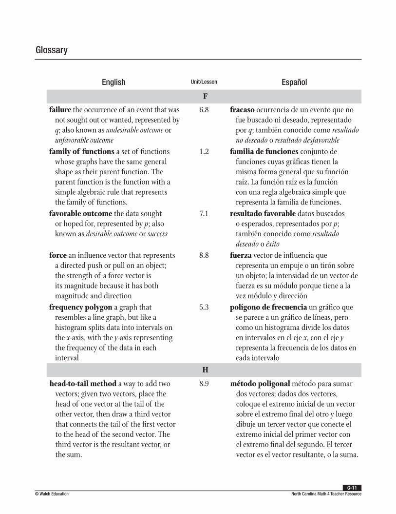
Glossary
English Unit/Lesson Español
F
failure the occurrence of an event that was not sought out or wanted, represented by q; also known as undesirable outcome or unfavorable outcome
6.8 fracaso ocurrencia de un evento que no fue buscado ni deseado, representado por q; también conocido como resultado no deseado o resultado desfavorable
family of functions a set of functions whose graphs have the same general shape as their parent function. The parent function is the function with a simple algebraic rule that represents the family of functions.
1.2 familia de funciones conjunto de funciones cuyas gráficas tienen la misma forma general que su función raíz. La función raíz es la función con una regla algebraica simple que representa la familia de funciones.
favorable outcome the data sought or hoped for, represented by p; also known as desirable outcome or success
7.1 resultado favorable datos buscados o esperados, representados por p; también conocido como resultado deseado o éxito
force an influence vector that represents a directed push or pull on an object; the strength of a force vector is its magnitude because it has both magnitude and direction
8.8 fuerza vector de influencia que representa un empuje o un tirón sobre un objeto; la intensidad de un vector de fuerza es su módulo porque tiene a la vez módulo y dirección
frequency polygon a graph that resembles a line graph, but like a histogram splits data into intervals on the x-axis, with the y-axis representing the frequency of the data in each interval
5.3 polígono de frecuencia un gráfico que se parece a un gráfico de líneas, pero como un histograma divide los datos en intervalos en el eje x, con el eje y representa la frecuencia de los datos en cada intervalo
H
head-to-tail method a way to add two vectors; given two vectors, place the head of one vector at the tail of the other vector, then draw a third vector that connects the tail of the first vector to the head of the second vector. The third vector is the resultant vector, or the sum.
8.9 método poligonal método para sumar dos vectores; dados dos vectores, coloque el extremo inicial de un vector sobre el extremo final del otro y luego dibuje un tercer vector que conecte el extremo inicial del primer vector con el extremo final del segundo. El tercer vector es el vector resultante, o la suma.
North Carolina Math 4 Teacher Resource
© Walch EducationG-11

Glossary
English Unit/Lesson Español
histogram a frequency plot that shows the number of times a response or range of responses occurred in a data set. Example:
5.3 6.1
histograma una diagrama de frecuencia que muestra la cantidad de veces que se produce una respuesta o rango de respuestas en un conjunto de datos. Ejemplo:
hypothesis a statement that you are trying to prove or disprove
5.4 hipótesis afirmación que usted intenta probar o desaprobar
I
identity matrix a square matrix that
has ones along the main diagonal and
zeros everywhere else. For example,
1 0 00 1 00 0 1
. When a matrix is
multiplied by an identity matrix, the
original matrix does not change.
8.6 8.7
matriz identidad matriz cuadrada que
tiene unos en la diagonal principal
y ceros en los demás lugares. Por
ejemplo,
1 0 00 1 00 0 1
. Cuando se
multiplica una matriz por la matriz
identidad, la matriz original no cambia.imaginary number any number of
the form bi, where b is a real number, i = −1 , and b ≠ 0
8.1 número imaginario cualquier número de la forma bi, en el que b es un número real, i = −1 , y b ≠ 0
imaginary unit, i the letter i, used to represent the non-real value, i = −1
8.1 unidad imaginaria, i la letra i, utilizada para representar el valor no real i = −1
North Carolina Math 4 Teacher Resource
© Walch EducationG-12

Glossary
English Unit/Lesson Español
included angle the angle between two sides
4.2 ángulo incluido ángulo entre dos lados
independent variable generally labeled on the x-axis; the quantity that changes based on values chosen
5.4 variable independiente generalmente designada en el eje x; cantidad que cambia según valores seleccionados
initial condition a constraint or limit on the domain or range of a function; a starting value that limits the function model in some way
1.1 condición inicial una restricción o límite en el dominio o rango de una función; un valor inicial que limita el modelo de función de alguna manera
initial point the point at which a vector begins; the “tail” of a vector
8.8 punto inicial punto en el cual comienza un vector; la “cola” de un vector
interval 1. the continuous set of real numbers between two given numbers 2. the set of all real numbers between two given numbers. The two numbers on the ends are the endpoints. The endpoints might or might not be included in the interval depending on whether the interval is open, closed, or half-open/half-closed.
6.3 intervalo 1. conjunto continuo de números reales entre dos números dados 2. conjunto de todos los números reales entre dos números dados. Los dos números en los finales son los extremos. Los extremos podrían o no estar incluidos en el intervalo, según si el intervalo está abierto, cerrado, o medio abierto o medio cerrado.
inverse matrix a matrix that when multiplied by the original matrix produces the identity matrix; also called the multiplicative inverse matrix. The inverse of matrix A is denoted A–1.
8.6 8.7
matriz inversa matriz que, cuando se la multiplica por la matriz original, produce la matriz identidad; también se la llama matriz inversa multiplicativa. La inversa de la matriz A se denota A–1.
L
Law of Cosines a formula for any triangle which states c2 = a2 + b2 – 2ab cos C, where C is the included angle in between sides a and b, and c is the nonadjacent side across from ∠C
4.3 Ley de Cosenos fórmula para todo triángulo que establece c2 = a2 + b2 – 2ab cos C, donde C es el ángulo incluido entre los lados a y b, y c es el lado no adyacente u opuesto ∠C
North Carolina Math 4 Teacher Resource
© Walch EducationG-13

Glossary
English Unit/Lesson Español
Law of Sines a formula for any triangle
which states = =a
A
b
B
c
Csin sin sin ,
where a represents the measure of
the side opposite ∠A, b represents the
measure of the side opposite ∠B , and
c represents the measure of the side
opposite ∠C
4.2 Ley de Senos fórmula para
todo triángulo que establece
= =a
A
b
B
c
Csin sin sin , donde a representa
la medida del lado opuesto ∠A, b
representa la medida del lado opuesto
∠B y c representa la medida del lado
opuesto ∠Clevel of confidence the probability
that a parameter’s value can be found in a specified interval; also called confidence level
7.2 grado de confianza probabilidad de que se pueda encontrar el valor de un parámetro en un intervalo específico; también llamado nivel de confianza
line graph a graph that shows how often each data value within a data set occurs; the horizontal axis represents data values, and the vertical axis shows the frequency of the data values. Points on the graph are connected by line segments.
5.3 gráfico lineal un gráfico que muestra la frecuencia con la que se produce cada valor de datos dentro de un conjunto de datos; el eje horizontal representa los valores de los datos y el eje vertical muestra la frecuencia de los valores de los datos. Los puntos del gráfico están conectados por segmentos de línea.
line symmetry exists for a figure if for every point on one side of the line of symmetry, there is a corresponding point the same distance from the line on the other side
4.5 simetría lineal la que existe en una figura si para cada punto a un lado de la línea de simetría, hay un punto correspondiente a la misma distancia de la línea
local maximum the greatest value of a function for a particular interval of the function; also known as a relative maximum
1.1 máximo local el mayor valor de una función para un intervalo específico de la función; también conocido como máximo relativo
local minimum the least value of a function for a particular interval of the function; also known as a relative minimum
1.1 mínimo local el menor valor de una función para un intervalo específico de la función; también conocido como mínimo relativo
North Carolina Math 4 Teacher Resource
© Walch EducationG-14

Glossary
English Unit/Lesson Español
logarithm a quantity that represents the power to which a base a must be raised in order to equal a quantity x; written loga x
3.1 logaritmo cantidad que representa la potencia a la cual se debe elevar una base a para que equivalga a una cantidad x; se escribe loga x
logarithmic function the inverse of an exponential function; for the exponential function f(x) = 5x, the inverse logarithmic function is x = log5 f(x)
3.1 función logarítmica la inversa de una función exponencial; para la función exponencial f(x) = 5x, la función logarítmica inversa es x = log5 f(x)
M
magnitude the length of a vector, denoted by v ; the length of vector
v a b,= is a b2 2v = +
8.8 módulo (de un vector) longitud de un vector, denotada por v ; la longitud
del vector v a b,= es a b2 2v = +margin of error the quantity that
represents the level of confidence in a calculated parameter, abbreviated MOE. The margin of error can be calculated by multiplying the critical value by the standard deviation, if known, or by the SEM.
7.2 margen de error cantidad que representa el nivel de confianza en un parámetro calculado, abreviado MOE. El margen de error puede calcularse multiplicando el valor crítico por la desviación estándar, si se conoce, o por el SEM.
matrix an ordered arrangement of numbers or expressions in rows and columns. The plural of matrix is matrices.
8.5 8.7
matriz arreglo de números o expresiones ordenado en filas y columnas. El plural de matriz es matrices.
mean the average value of a data set, found by summing all values and dividing by the number of data points
6.3 media valor promedio de un conjunto de datos, que se determina al sumar todos los valores y dividirlos por la cantidad de puntos de datos
median the middle-most value of a data set; 50% of the data is less than this value, and 50% is greater than it
6.4 mediana valor medio exacto de un conjunto de datos; el 50% de los datos es menor que ese valor, y el otro 50% es mayor
midline in a cosine function or sine function of the form f(x) = a + sin x or g(x) = a + cos x, a horizontal line of the form y = a that bisects the vertical distance on a graph between the minimum and maximum function values
4.5 línea media en una función del coseno o en una función del seno de la forma f(x) = a + sin x o g(x) = a + cos x, una línea horizontal de la forma y = a que divide en dos la distancia vertical en un gráfico entre los valores de funciones mínimos y máximos
North Carolina Math 4 Teacher Resource
© Walch EducationG-15

Glossary
English Unit/Lesson Español
modulus the square root of the product of a complex number and its conjugate. The modulus is the absolute value of a complex number.
8.4 módulo (de un número complejo) es la raíz cuadrada del producto de un número complejo y su conjugado. El módulo es el valor absoluto de un número complejo.
mu, µ a Greek letter used to represent mean
6.3 mu, µ letra griega usada para representar la media
multiplication rule for independent events The probability of two independent events A and B both occurring is P(A and B) = P(A) • P(B).
6.7 regla de multiplicación para eventos independientes La probabilidad de que dos eventos independientes A y B ocurran ambos es P(A y B) = P(A) • P(B).
multiplicative identity the element of a set whose multiplication does not change other elements; the multiplicative identity of the real numbers is 1
8.7 identidad de la multiplicación el elemento de un conjunto cuya multiplicación no cambia a los demás elementos; la identidad de la multiplicación en los números reales es el 1
multiplicative identity matrix a matrix
that has ones along the main diagonal
and zeros everywhere else; also called
the identity matrix. For example,
1 0 00 1 00 0 1
; represented as I. When
a matrix is multiplied by an identity
matrix, the original matrix does not
change.
8.7 matriz identidad para la multiplicación
matriz que tiene unos en la diagonal
principal y ceros en los demás lugares;
también se la llama matriz identidad.
Por ejemplo, 1 0 00 1 00 0 1
, que
se representa como I. Cuando se
multiplica una matriz por la matriz
identidad, la matriz original no cambia.
North Carolina Math 4 Teacher Resource
© Walch EducationG-16

Glossary
English Unit/Lesson Español
multiplicative inverse matrix a matrix that when multiplied by the original matrix produces the identity matrix; also called the inverse matrix. The inverse of matrix A is denoted A–1.
8.7 matriz inversa multiplicativa matriz que, cuando se la multiplica por la matriz original, produce la matriz identidad; también se la llama matriz inversa. La inversa de la matriz A se denota A–1.
mutually exclusive events events that have no outcomes in common. If A and B are mutually exclusive events, then they cannot both occur.
6.8 eventos mutuamente excluyentes eventos que no tienen resultados en común. Si A y B son eventos mutuamente excluyentes, entonces no pueden producirse ambos.
N
natural logarithm a logarithm whose base is the irrational number e; usually written in the form “ln,” which means “loge”
3.1 logaritmo natural logaritmo cuya base es el número irracional e; escrito normalmente en la forma “ln,” que significa “loge”
negatively skewed a distribution in which there is a “tail” of isolated, spread-out data points to the left of the median. “Tail” describes the visual appearance of the data points in a histogram. Data that is negatively skewed is also called skewed to the left.
6.1 6.5
sesgado negativamente distribución en la cual existe una “cola” de puntos de datos aislados y esparcidos a la izquierda de la mediana. La “cola” describe la apariencia visual de los puntos de datos en un histograma. Los datos que están sesgados negativamente también se denominan sesgados a la izquierda.
non-ordinal data data that is categorical, but with no obvious ordering to the categories; for example, data sorted by hair color
5.3 datos no ordinales datos categóricos, pero sin un orden obvio de las categorías; por ejemplo, datos ordenados por color de cabello
normal curve a symmetrical curve representing the normal distribution
6.3 curva normal curva simétrica que representa la distribución normal
normal distribution a set of values that are continuous, are symmetric to a mean, and have higher frequencies in intervals close to the mean than equal-sized intervals away from the mean
6.1 distribución normal conjunto de valores que son continuos, simétricos a una media y tienen frecuencias más altas en intervalos cercanos a la media que los intervalos de igual tamaño lejos de la media
North Carolina Math 4 Teacher Resource
© Walch EducationG-17

Glossary
English Unit/Lesson Español
normal probability distribution a probability distribution whose graph is symmetric and is shaped like a bell; most of the data are near or at the mean
6.1 distribución de probabilidad normal distribución de probabilidad cuya gráfica es simétrica y con forma de campana; la mayoría de los datos están cerca de la media o en la media
O
oblique triangle a triangle that does not contain a right angle
4.3 triángulo oblicuo triángulo que no contiene un ángulo recto
odd function a function that, when evaluated for –x, results in a function that is the opposite of the original function; f(–x) = –f(x)
1.3 4.5
función impar función que, cuando se evalúa para –x, tiene como resultado una función que es lo opuesto a la función original; f(–x) = –f(x)
opposite matrix the matrix which, when added to matrix A, yields the zero matrix; also called the additive inverse matrix. The opposite of matrix A is –A.
8.7 matriz opuesta es la matriz que, cuando se la suma a la matriz A, el resultado es la matriz cero; también se la llama matriz inversa aditiva. La opuesta a la matriz A es –A.
ordinal data categorical data sorted with a clear order; for example, data sorted by age or month
5.3 datos ordinales datos categóricos ordenados con un orden claro; por ejemplo, datos ordenados por edad o mes
outlier a data value that is much greater than or much less than the rest of the data in a data set; mathematically, any data less than Q 1 – 1.5(IQR) or greater than Q 3 + 1.5(IQR) is an outlier
6.5 valor atípico valor de datos que es mucho mayor o mucho menor que el resto de los datos de un conjunto de datos; en matemática, cualquier dato menor que Q 1 – 1,5(IQR) o mayor que Q 3 + 1,5(IQR) es un valor atípico
P
Parallelogram Rule a method for vector addition; when the initial points of two vectors u and v are aligned, they define a parallelogram whose diagonal represents the vector sum u v +
8.9 regla del paralelogramo método de suma de vectores; cuando se alinean los extremos iniciales de dos vectores u y v , definen un paralelogramo cuya diagonal representa al vector suma u v +
parent function a function with a simple algebraic rule that represents a family of functions. The graphs of the functions in the family have the same general shape as the parent function.
1.3 función principal función con una regla algebraica simple que representa una familia de funciones. Los gráficos de las funciones en la familia tienen la misma forma general que la función principal.
North Carolina Math 4 Teacher Resource
© Walch EducationG-18

Glossary
English Unit/Lesson Español
period in the graph of a trigonometric function, the horizontal distance from the beginning to the end of a cycle
4.5 período en la gráfica de una función trigonométrica, es la distancia horizontal desde el principio hasta el final de un ciclo
periodic function a function whose values repeat at regular intervals
1.1 4.5
función periódica función cuyos valores se repiten a intervalos regulares
phase shift for the graph of a trigonometric function, the horizontal distance by which the curve of a parent function is shifted by the addition of a constant or other expression in the argument of the function
4.5 cambio de fase en la gráfica de una función trigonométrica es la distancia horizontal por la cual se cambia la curva de una función madre mediante la adición de una constante u otra expresión en el argumento de la función
piecewise function a function that is defined by two or more expressions on separate portions of the domain
2.1 función por partes función definida por dos o más expresiones en porciones separadas del dominio
point of symmetry a central point such that if a graph is rotated 180° about the point, the resulting graph will look exactly like the original graph
4.5 punto de simetría punto central tal que si una gráfica se rota 180° con relación a ese punto, la gráfica que se obtiene es exactamente igual a la original
population all of the people, objects, or phenomena of interest in an investigation; the entire data set
6.3 población todas las personas, los objetos o fenómenos de interés en una investigación; el conjunto completo de datos
population average the sum of all quantities in a population, divided by the total number of quantities in the population; typically represented by µ; also known as population mean
7.1 promedio de la población suma de todas las cantidades de una población, dividida por el número total de cantidades de la población; representada normalmente por µ; también se conoce como media poblacional
population mean the sum of all quantities in a population, divided by the total number of quantities in the population; typically represented by µ; also known as population average
7.1 media poblacional suma de todas las cantidades de una población, dividida por el número total de cantidades de la población; representada normalmente µ; también se conoce como promedio de la población
North Carolina Math 4 Teacher Resource
© Walch EducationG-19

Glossary
English Unit/Lesson Español
positively skewed a distribution in which there is a “tail” of isolated, spread-out data points to the right of the median. “Tail” describes the visual appearance of the data points in a histogram. Data that is positively skewed is also called skewed to the right.
6.1 6.5
sesgado positivamente distribución en la cual existe una “cola” de puntos de datos aislados esparcidos hacia la derecha de la mediana. La “cola” describe la apariencia de los puntos de datos en un histograma. Los datos que están positivamente sesgados también se denominan sesgados a la derecha.
probability distribution an equation, table, or graph that maps each element in the sample space (possible outcomes) to the probability that it will occur
6.1 6.2 6.3 6.6
distribución de probabilidad ecuación, tabla o gráfica que asigna a cada elemento del espacio de muestra (resultados posibles) a la probabilidad de que ocurra
Pythagorean identities trigonometric identities that are derived from the Pythagorean Theorem: sin2θ + cos2θ = 1, 1 + tan2θ = sec2θ, and 1 + cot2θ = csc2θ
4.1 identidades Pitagóricas identidades trigonométricas que se derivan de el teorema de Pitágoras: sen2θ + cos2θ = 1, 1 + tan2θ = sec2θ, and 1 + cot2θ = csc2θ
Pythagorean Theorem a theorem that relates the length of the hypotenuse of a right triangle (c) to the lengths of its legs (a and b). The theorem states that a2 + b2 = c2.
4.1 Teorema de Pitágoras teorema que relaciona la longitud de la hipotenusa de un triángulo rectángulo (c) con las longitudes de sus catetos (a y b). El teorema establece que a2 + b2 = c2.
Q
quantitative data anything that is counted or measured
5.3 datos cuantitativos cualquier cosa que se cuente o mida
R
random sample a subset or portion of a population or set that has been selected without bias, with each item in the population or set having the same chance of being found in the sample
5.1 muestra aleatoria subconjunto o porción de población o conjunto que ha sido seleccionado sin sesgo, con cada elemento de la población o conjunto con la misma probabilidad de encontrarse en la muestra
random variable a variable whose numerical value changes depending on each outcome in a sample space; the values of a random variable are associated with chance variation
6.1 6.2 6.3
variable aleatoria variable cuyo valor numérico cambia según cada resultado en un espacio de muestra; los valores de una variable aleatoria están asociados con una variación al azar
North Carolina Math 4 Teacher Resource
© Walch EducationG-20

Glossary
English Unit/Lesson Español
range the set of all outputs of a relation or function; the set of y-values for which a function is defined
4.5 rango conjunto de todas las salidas de una función; conjunto de valores de y para el que se define una función
ratio identities identities that define tangent and cotangent in terms of
sine and cosine: tansin
cosθ
θθ
= and
cotcos
sinθ
θθ
=
4.1 identidades de proporciones identidades que definen tangente y
cotangente en términos de seno y el
coseno: tansen
cosθ
θθ
= y cotcos
senθ
θθ
=
reciprocal identities trigonometric identities that define cosecant, secant, and cotangent in terms of sine, cosine,
and tangent: csc1
sinθ
θ= , sec
1
cosθ
θ= ,
cot1
tanθ
θ= , sin
1
cscθ
θ= , cos
1
secθ
θ= ,
and tan1
cotθ
θ=
4.1 identidades recíprocas identidades trigonométricas que definen cosecante, secante y cotangente en términos de
seno, coseno y tangente: csc1
senθ
θ= ,
seccos
θθ
=1
, cottan
θθ
=1
,
sen1
csc, cos
1
sec, y tan
1
cotθ
θθ
θθ
θ= = =
reference angle the acute angle that
the terminal side of an angle in
standard position makes with the
x-axis, expressed as a positive value
less than or equal to 2
π radians or 90°.
The sine, cosine, and tangent of the
reference angle are the same as those
of the original angle (except for the
sign, which is based on the quadrant in
which the terminal side is located).
4.5 ángulo de referencia ángulo agudo que
forma con el eje x el lado terminal de un
ángulo en posición estándar, expresado
como un valor positivo menor o igual a
2
π radianes o a 90°. El seno, el coseno y
la tangente del ángulo de referencia son
iguales a los del ángulo original (con
excepción del signo, que se basa en el
cuadrante en el que se ubica el lado
terminal).reflection matrix a matrix which, when
multiplied on the left of a vector, yields a vector that is a reflection of the input vector
8.7 matriz de reflejo matriz que, cuando se la multiplica a izquierda por un vector, se obtiene un vector que es el reflejo del original
North Carolina Math 4 Teacher Resource
© Walch EducationG-21

Glossary
English Unit/Lesson Español
regression the function being fitted to the data in a regression analysis; also know as a regression model
2.4 3.5 4.6
regresión la función que se ajusta a los datos en un análisis de regresión; también conocido como modelo de regresión
regression analysis a set of statistical processes that fit a particular function model to a data set
2.4 3.5 4.6
análisis de regresión un conjunto de procesos estadísticos que ajustan un modelo de función particular a un conjunto de datos
regression model the function being fitted to the data in a regression analysis; also know as regression
2.4 3.5
modelo de regresión la función se ajusta a los datos en un análisis de regresión; también conocido como regresión
relative maximum the greatest value of a function for a particular interval of the function; also known as a local maximum
1.1 máximo relativo el mayor valor de una función para un intervalo en particular de la función; también conocido como máximo local
relative minimum the least value of a function for a particular interval of the function; also known as a local minimum
1.1 mínimo relativo el menor valor de una función para un intervalo en particular de la función; también conocido como mínimo local
residual the vertical distance between an observed data value and an estimated data value on a line of best fit
2.5 4.6
residual distancia vertical entre un valor de datos observado y un valor de datos estimado sobre una línea de ajuste óptimo
residual plot provides a visual representation of the residuals for a set of data; contains the points (x, residual for x)
2.5 3.5 4.6
diagrama residual brinda una representación visual de los residuales para un conjunto de datos; contiene los puntos (x, residual de x)
resultant vector the result of vector addition; adding vectors u and v yields the resultant vector u v +
8.9 vector resultante es el resultado de la sumatoria de vectores; al sumar los vectores u y v , se obtiene el vector resultante u v +
rotation matrix a matrix which, when multiplied on the left of a vector, yields a vector that is a rotation of the input vector
8.7 matriz de rotación matriz que, cuando se la multiplica a izquierda por un vector, se obtiene un vector que es una rotación del original
row an arrangement of data in a horizontal line
8.5 fila arreglo de datos en línea horizontal
North Carolina Math 4 Teacher Resource
© Walch EducationG-22

Glossary
English Unit/Lesson Español
S
sample a subset of the population 6.3 muestra subconjunto de la población
sample average the sum of all quantities in a sample divided by the total number of quantities in the sample, typically represented by x ; also known as sample mean
7.1 promedio de la muestra suma de todas las cantidades en una muestra dividida por el número total de cantidades en la muestra, normalmente representada por x ; también se conoce como media de la muestra
sample mean the sum of all quantities in a sample divided by the total number of quantities in the sample, typically represented by x ; also known as sample average
7.1 media de la muestra suma de todas las cantidades en una muestra dividida por el número total de cantidades en la muestra, normalmente representada por x ; también se conoce como promedio de la muestra
sample population a portion of the population; the number of elements or observations in a sample population is represented by n
7.1 población de la muestra porción de la población; la cantidad de elementos u observaciones en una población de muestra se representa por n
sample proportion the fraction of
favorable results p from a sample
population n; conventionally
represented by p̂, which is pronounced
“p hat.” The formula for the sample
proportion is ˆ =pp
n, where p is
the number of favorable outcomes
and n is the number of elements or
observations in the sample population.
7.1 proporción de la muestra fracción
de los resultados favorables p
de una población de muestra n;
convencionalmente representada por p̂,
que se pronuncia “p hat”. La fórmula
para la proporción de la muestra es
ˆ =pp
n, donde p es la cantidad de
resultados favorables y n es la cantidad
de elementos u observaciones en la
población de la muestra.
sample size the number of members of a population that participate in a survey
5.2 tamaño de la muestra el número de miembros de una población que participan en una encuesta
North Carolina Math 4 Teacher Resource
© Walch EducationG-23

Glossary
English Unit/Lesson Español
sampling bias errors in estimation caused by flawed (non-representative) sample selection
5.1 sesgo de muestreo errores de cálculo ocasionados por una selección defectuosa (no representativa) de la muestra
scalar a quantity, usually a constant; a numerical quantity without an associated direction
8.5 8.8
escalar una cantidad, por lo general una constante; cantidad numérica sin dirección asociada
scatter plot a graph of data in two variables on a coordinate plane, where each data pair is represented by a point
2.4 diagrama de dispersión gráfica de datos en dos variables en un plano de coordenadas, en la que cada par de datos está representado por un punto
selective sampling a method in which the sample is selected with particular participants in mind in order to purposefully introduce bias
5.2 muestreo selectivo un método en el que la muestra se selecciona teniendo en cuenta a determinados participantes con el fin de introducir sesgos a propósito
sigma (lowercase), σ a Greek letter used to represent standard deviation
6.3 sigma (minúscula) o σ letra griega utilizada para representar la desviación estándar
sigma (uppercase), ∑ a Greek letter used to represent the summation of values
6.4 sigma (mayúscula) o ∑ letra griega utilizada para representar la sumatoria de valores
simple random sample a sample in which any combination of a given number of individuals in the population has an equal chance of selection
5.1 muestra aleatoria simple muestra en la cual cualquier combinación de una cantidad dada de individuos de la población tiene iguales posibilidades de selección
simple random sampling (SRS) a sampling method in which each member in a population has an equal probability of being selected for a sample, and individuals are picked at random
5.2 muestreo aleatorio simple un método de muestreo en el que cada miembro de una población tiene la misma probabilidad de ser seleccionado para una muestra, y los individuos se seleccionan al azar
North Carolina Math 4 Teacher Resource
© Walch EducationG-24

Glossary
English Unit/Lesson Español
simulation a set of data that models an event that could happen in real life
7.3 simulación conjunto de datos que imita un evento que podría suceder en la vida real
sinusoidal regression a sine curve that has been fitted to a data set
4.6 regresión sinusoidal una curva sinusoidal que se ha ajustado a un conjunto de datos
skewed to the left a distribution in which there is a “tail” of isolated, spread-out data points to the left of the median. “Tail” describes the visual appearance of the data points in a histogram. Data that is skewed to the left is also called negatively skewed.
6.1 6.5
sesgado a la izquierda distribución en la cual existe una “cola” de puntos de datos aislados extendidos hacia la izquierda de la mediana. La “cola” describe la apariencia de los puntos de datos en un histograma. Los datos sesgados a la izquierda también se denominan negativamente sesgados.
skewed to the right a distribution in which there is a “tail” of isolated, spread-out data points to the right of the median. “Tail” describes the visual appearance of the data points in a histogram. Data that is skewed to the right is also called positively skewed.
6.1 6.5
sesgado a la derecha distribución en la cual existe una “cola” de puntos de datos aislados extendidos hacia la derecha de la mediana. La “cola” describe la apariencia de los puntos de datos en un histograma. Los datos sesgados a la derecha también se denominan positivamente sesgados.
special angles angles with a reference
angle of 0°, 30°, 45°, 60°, or 90°
(or 0, 6
π ,
4
π,
3
π, or
2
π radians);
angles whose trigonometric values can
be computed exactly
4.5 ángulos especiales ángulos con un
ángulo de referencia de 0°, 30°, 45°, 60°
o 90° (o 0, 6
π ,
4
π,
3
π o
2
π radianes);
ángulos cuyos valores trigonométricos
se pueden calcular de manera exacta
speed the magnitude of an object’s velocity vector
8.8 velocidad módulo del vector velocidad de un objeto
square matrix a matrix with the same number of rows and columns
8.6 8.7
matriz cuadrada matriz con la misma cantidad de filas y columnas
North Carolina Math 4 Teacher Resource
© Walch EducationG-25

Glossary
English Unit/Lesson Español
standard deviation how much the data
in a given set is spread out, represented
by s or σ. The standard deviation
of a sample can be found using the
following formula: 1
2∑( )=
−−
sx x
ni .
The standard deviation of a population
can be found using the following
formula: x
n
ii
n
( )2
1∑
σµ
=−
= .
6.3 desviación estándar cuánto se
extienden los datos en un conjunto
dado, representada por s o σ. Se puede
calcular la desviación estándar de
una muestra utilizando la siguiente
fórmula: 1
2∑( )=
−−
sx x
ni . Se puede
calcular la desviación estándar de
una población utilizando la siguiente
fórmula: x
n
ii
n
( )2
1∑
σµ
=−
= .
standard error an estimate of how far a sample statistic likely lies from the actual population statistic
7.1 error estándar una estimación de a qué distancia una estadística de la muestra probablemente está de la estadística demográfica actual
standard error of the mean the
variability of the mean of a sample;
given by SEM =s
n, where s represents
the standard deviation and n is the
number of elements or observations in
the sample population
7.1 error estándar de la media variabilidad
de la media de una muestra; dado
por SEM =s
n, donde s representa
la desviación estándar y n la cantidad
de elementos u observaciones en la
población de la muestra
North Carolina Math 4 Teacher Resource
© Walch EducationG-26

Glossary
English Unit/Lesson Español
standard error of the proportion the
variability of the measure of the
proportion of a sample, abbreviated
SEP. The standard error (SEP) of a
sample proportion p̂ is given by the
formula SEPˆ 1 ˆ( )
=−p p
n, where p̂
is the sample proportion determined
by the sample and n is the number of
elements or observations in the sample
population.
7.1 error estándar de la proporción
variabilidad de la medida de la
proporción de una muestra, abreviada
SEP. El error estándar (SEP) de una
proporción de la muestra p̂ está dado
por la fórmula SEPˆ 1 ˆ( )
=−p p
n, donde
p̂ es la proporción de la muestra
determinada por la muestra y n
representa la cantidad de elementos
u observaciones en la población de la
muestra.standard normal distribution
a normal distribution that has a mean of 0 and a standard deviation of 1; data following a standard normal distribution forms a normal curve when graphed
6.3 distribución normal estándar distribución normal que tiene una media de 0 y una desviación estándar de 1; los datos que siguen una distribución normal estándar forman una curva normal al graficarse
statistical reports reports that communicate findings from data analysis
5.5 informes estadísticos informes que comunican los resultados del análisis de datos
stem-and-leaf plot a graph used to display quantitative data, generally from small data sets, by dividing the data into a “stem” column (usually the leading digits of the data) and a “leaf ” column (the remaining digits)
5.3 diagrama de tallo y hojas un gráfico que se utiliza para mostrar datos cuantitativos, generalmente de pequeños conjuntos de datos, dividiendo los datos en una columna de “tallo” (generalmente los dígitos iniciales de los datos) y una columna de “hoja” (los dígitos restantes)
North Carolina Math 4 Teacher Resource
© Walch EducationG-27

Glossary
English Unit/Lesson Español
step function a function that is a series of disconnected constant functions
2.1 función escalonada función que es una serie de funciones constantes desconectadas
stratified random sampling a method for selecting members of a population through first grouping and then using simple random sampling to select individuals from each group
5.2 muestreo aleatorio estratificado un método para seleccionar miembros de una población a través del primer agrupamiento y luego usando un muestreo aleatorio simple para seleccionar individuos de cada grupo
success the data sought or hoped for, represented by p; also known as desirable outcome or favorable outcome
7.1 éxito datos buscados o esperados, representados por p; también conocido como resultado deseado o resultado favorable
summary statistics information that provides a quick description of a data set as a whole; can include the mean, median, mode, range, expected value, and standard deviation
6.2 resumen estadístico información que describe brevemente un conjunto de datos como un todo; puede incluir la media, la mediana, la moda, el rango, el valor esperado y la desviación estándar
summation notation a symbolic way to represent a series (the sum of a sequence) using the uppercase Greek letter sigma, ∑
6.4 notación sumatoria forma simbólica de representar una serie (la suma de una secuencia) utilizando la letra griega mayúscula sigma, ∑
supplementary angles two angles whose sum is 180° or π radians
4.5 ángulos suplementarios dos ángulos cuya suma es 180° o π radianes
symmetric distribution a data distribution in which a line can be drawn so that the left and right sides are mirror images of each other
6.4 distribución simétrica distribución de datos en la cual se puede trazar una línea de manera que los lados derecho e izquierdo sean imágenes especulares entre sí
symmetry of a function the property whereby a function exhibits the same behavior (e.g., graph shape, function values, etc.) for specific domain values and their opposites
1.1 simetría de una función propiedad por la cual una función exhibe el mismo comportamiento (por ej., forma de la gráfica, valores de la función, etc.) para valores específicos del dominio y sus opuestos
North Carolina Math 4 Teacher Resource
© Walch EducationG-28

Glossary
English Unit/Lesson Español
systematic sample a sample drawn by selecting people or objects from a list, chart, or grouping at a uniform interval; for example, selecting every fourth person
5.2 muestra sistemática la muestra se obtiene mediante la selección de personas u objetos a partir de una lista, una tabla o mediante la agrupación a intervalos regulares; por ej., eligiendo una de cada cuatro personas
system of equations a set of equations with the same unknowns
8.6 sistema de ecuaciones conjunto de ecuaciones con las mismas incógnitas
T
terminal point the point at which a vector ends; the “head” of a vector
8.8 extremo final punto en el cual termina un vector; es el extremo “con la punta de flecha”
theoretical probability the probability that an outcome will occur as determined through reasoning or calculation, given by the formula
P EE
( )number of outcomes in
number of outcomes in the sample space=
6.6 probabilidad teórica probabilidad de que un resultado se produzca como se determinó mediante razonamiento o cálculo, dado por la fórmula
( )cantidad de resultados en E
cantidad de resultados en el espacio de muestreoP E =
time series graph a graph that sorts data values by the time each value was recorded. The graph is a Cartesian plane with time measured on the horizontal axis and data values on the vertical axis. Points are typically plotted in chronological order and connected with line segments.
5.3 gráfica de series de tiempo un gráfico que ordena los valores de datos por el momento en que se registró cada valor. El gráfico es un plano cartesiano con tiempo medido en el eje horizontal y valores de datos en el eje vertical. Los puntos generalmente se trazan en orden cronológico y se conectan con segmentos de línea.
transformation matrix a matrix with special properties that can be used to rotate, reflect, or dilate a vector
8.7 matriz de transformación matriz con propiedades especiales que se puede usar para rotar un vector, reflejarlo o cambiar su escala
translation moving a graph or figure either vertically, horizontally, or both, without changing its shape; a slide
8.6 traslación movimiento de un gráfico en sentido vertical, horizontal, o en ambos, sin modificar su forma; deslizamiento
North Carolina Math 4 Teacher Resource
© Walch EducationG-29

Glossary
English Unit/Lesson Español
treatment the process or intervention provided to the population being observed
5.4 tratamiento proceso o intervención efectuada sobre la población que está siendo observada
trial each individual event or selection in an experiment or treatment
6.8 ensayo cada evento o selección individual en un experimento o tratamiento
U
undesirable outcome the data not sought or hoped for, represented by q; also known as unfavorable outcome or failure
6.8 resultado no deseado datos no buscados o esperados, representados por q; también conocido como resultado desfavorable o fracaso
unfavorable outcome the data not sought or hoped for, represented by q; also known as undesirable outcome or failure
6.8 resultado desfavorable datos no buscados o esperados, representados por q; también conocido como resultado no deseado o fracaso
uniform distribution a set of values that are continuous, are symmetric to a mean, and have equal frequencies corresponding to any two equally sized intervals. In other words, the values are spread out uniformly throughout the distribution.
6.3 distribución uniforme conjunto de valores que son continuos, simétricos respecto de la media y tienen frecuencias iguales que corresponden a cualquiera de dos intervalos del mismo tamaño. En otras palabras, los valores se extienden uniformemente en la distribución.
uniform probability distribution a probability distribution in which the possible outcomes of a statistical experiment occur with equal probability
6.1 distribución de probabilidad uniforme distribución de probabilidad en la cual los resultados posibles de un experimento estadístico ocurren con igual probabilidad
unit vector a vector with magnitude 1.
Given any vector v , the scalar multiple v
v is the unique unit vector that
points in the same direction as v .
8.9 vector unitario vector de módulo 1. Dado
cualquier vector v , el múltiplo escalar v
v es el único vector unitario que
apunta en la misma dirección que v .
North Carolina Math 4 Teacher Resource
© Walch EducationG-30
Glossary
English Unit/Lesson Español
V
vector a quantity having both direction and magnitude
8.8 vector cantidad que tiene tanto dirección como módulo
velocity vector a vector that represents the motion of an object
8.8 vector velocidad vector que representa el movimiento de un objeto
vertex of a cone the point of a cone; also referred to as the apex
4.2 vértice de un cono es la punta de un cono; también se lo llama cúspide
vertical displacement the amount by which the graph of a trigonometric function is moved up or down. If f(x) = c sin(ax + b) + d, the vertical displacement is d.
4.5 desplazamiento vertical la cantidad por la cual la gráfica de una función trigonométrica se mueve hacia arriba o hacia abajo. Si f(x) = c sin(ax + b) + d, el desplazamiento vertical es d.
W
weighted average a type of arithmetic mean in which some elements carry more importance (weight) than others. This number is calculated by multiplying each element by a number that represents the element’s relative importance or weight.
6.2 promedio ponderado tipo de media aritmética en la cual a algunos elementos se les asigna más importancia (peso) que a otros. Para calcular este valor, se multiplica cada elemento por un número que representa la importancia relativa o peso del elemento.
wholly imaginary a complex number that has a real part equal to 0; written in the form a + bi, where a and b are real numbers, i is the imaginary unit, a = 0, and b ≠ 0: 0 + bi
8.1 totalmente imaginario número complejo que tiene una parte real igual a 0; se expresa en la forma a + bi, donde a y b son números reales, i es la unidad imaginaria, a = 0, y b ≠ 0: 0 + bi
wholly real a complex number that has an imaginary part equal to 0; written in the form a + bi, where a and b are real numbers, i is the imaginary unit, b = 0, and a ≠ 0: a + 0i
8.1 totalmente real número complejo que tiene una parte imaginaria igual a 0; se expresa en la forma a + bi, donde a y b son números reales, i es la unidad imaginaria, b = 0, y a ≠ 0: a + 0i
North Carolina Math 4 Teacher Resource
© Walch EducationG-31

Glossary
North Carolina Math 4 Teacher Resource
© Walch EducationG-32
English Unit/Lesson Español
Z
z-score the number of standard deviations that a score lies above or below the mean; given by the formula
zx µσ
=−
6.4 puntuación z cantidad de desviaciones estándar por encima o por debajo de la media que presenta la muestra; dada
por la fórmula zx µσ
=−
zc-value a measure of the number of standards of error to be added to or subtracted from the mean in order to achieve the desired confidence level; also known as critical value
7.2 valor zc medida de la cantidad de estándares de error que se suma o se resta de la media para lograr el nivel de confianza deseado; también conocido como valor crítico
zero matrix a matrix for which all entries are 0; the matrix whose addition does not change other matrices. Also known as the additive identity matrix.
8.7 matriz cero es una matriz cuyas entradas son todas 0; es la matriz cuya sumatoria no cambia a las demás matrices. También se la conoce como matriz identidad de la suma.

Teacher ResourceUnit 2: Piecewise Functions, Composition of Functions,
and Regression
North Carolina Math 4

© Common Core State Standards. Copyright 2010. National Governor’s Association Center for Best Practices and
Council of Chief State School Officers. All rights reserved.
1 2 3 4 5 6 7 8 9 10
ISBN 978-0-8251-9066-7
Copyright © 2020
J. Weston Walch, Publisher
Portland, ME 04103
www.walch.com
Printed in the United States of America
The classroom teacher may reproduce these materials for classroom use only.The reproduction of any part for an entire school or school system is strictly prohibited.
No part of this publication may be transmitted, stored, or recorded in any formwithout written permission from the publisher.
This program was developed and reviewed by experienced math educators who have both academic and professional backgrounds in mathematics. This ensures: freedom from mathematical errors, grade level
appropriateness, freedom from bias, and freedom from unnecessary language complexity.
Developers and reviewers include:
Jasmine Owens
Joanne N. Whitley
Shelly Northrop Sommer
Joyce Hale
Ruth Estabrook
Pam Loveridge
James Gunnin
Robert Leichner
Joseph Nicholson
Kristine Chiu
Chris Moore
Kaitlyn Hollister
Samantha Carter
Dawn McNair
Jack Loynd
Terri Germain-Williams
Laura McPartland
David Rawson
Lenore Horner
Nancy Pierce
Dale Blanchard
Pamela Rawson
Valerie Ackley
Lynze Greathouse
Jane Mando
Timothy Trowbridge
Alan Hull
Angela Heath
Linda Kardamis
Cameron Larkins
Frederick Becker
Kimberly Brady
Corey Donlan
Pablo Baques
Mike May, S.J.
Whit Ford
Heather Morton
Deborah Benton
Erin Brack
Kim Brady

Unit 2: Piecewise Functions, Composition of Functions, and RegressionUnit 2 Resources . . . . . . . . . . . . . . . . . . . . . . . . . . . . . . . . . . . . . . . . . . . . . . . . . . . . . . . . . . . . . . . . . . . . U2-1
Lesson 2.1: Piecewise, Step, and Absolute Value Functions (NC.M4.AF.4.1, NC.M4.AF.4.2) . . . . U2-5Lesson 2.2: Composition of Functions (NC.M4.AF.1.1) . . . . . . . . . . . . . . . . . . . . . . . . . . . . . . . . U2-33Lesson 2.3: Evaluating Composite Functions in Various Forms (NC.M4.AF.1.2) . . . . . . . . . . . U2-56Lesson 2.4: Linear, Exponential, and Quadratic Regression (NC.M4.AF.5.1) . . . . . . . . . . . . . . U2-81Lesson 2.5: Analyzing Residual Plots (NC.M4.AF.5.2) . . . . . . . . . . . . . . . . . . . . . . . . . . . . . . . . U2-112
Answer Key . . . . . . . . . . . . . . . . . . . . . . . . . . . . . . . . . . . . . . . . . . . . . . . . . . . . . . . . . . . . . . . . . . . . . . . U2-155
Mid-Unit Assessment and Answer Key . . . . . . . . . . . . . . . . . . . . . . . . . . . . . . . . . . . . . . . . . . . . . . . MA-1
End-of-Unit Assessment and Answer Key . . . . . . . . . . . . . . . . . . . . . . . . . . . . . . . . . . . . . . . . . . . . . . EA-1
North Carolina Math 4 Teacher Resource
© Walch Education
Table of Contents
iii


Unit 2 ResourcesInstruction
UNIT 2 • PIECEWISE FUNCTIONS, COMPOSITION OF FUNCTIONS, AND REGRESSION
North Carolina Math 4 Teacher Resource Unit 2 Resources
© Walch Education
Essential Questions
1. How do you decide what restrictions exist on the domain and range variables in a model that represents a real-world problem and/or its solution?
2. How do you sketch a function model so that it represents the relationships in a real-world problem?
3. What function results when you use a function, f(x), as the independent variable in another function, g(x)?
4. What are some real-world applications of the composition of functions?
5. How can a composition of functions be evaluated for a specific value?
6. What is regression analysis?
7. How can it be determined graphically that a line is a good estimate for a data set?
8. How do you interpret the features of a data plot that will determine what kind of function should be used to model the data?
9. What does a residual plot display?
10. How can a residual plot help determine whether a function is a good estimate for a data set?
11. Is the regression model with the nicest residual plot always the best choice?
North Carolina Math 4 Standards
NC.M4.AF.1.1 Execute algebraic procedures to compose two functions.
NC.M4.AF.1.2 Execute a procedure to determine the value of a composite function at a given value when the functions are in algebraic, graphical, or tabular representations.
NC.M4.AF.4.1 Translate between algebraic and graphical representations of piecewise functions (linear, exponential, quadratic, polynomial, square root).
NC.M4.AF.4.2 Construct piecewise functions to model a contextual situation.
NC.M4.AF.5.1 Construct regression models of linear, quadratic, exponential, logarithmic, and sinusoidal functions of bivariate data using technology to model data and solve problems.
NC.M4.AF.5.2 Compare residuals and residual plots of non-linear models to assess the goodness-of-fit of the model.
U2-1
SMP 1 ✓ 2 ✓3 ✓ 4 ✓5 ✓ 6 ✓7 ✓ 8 ✓
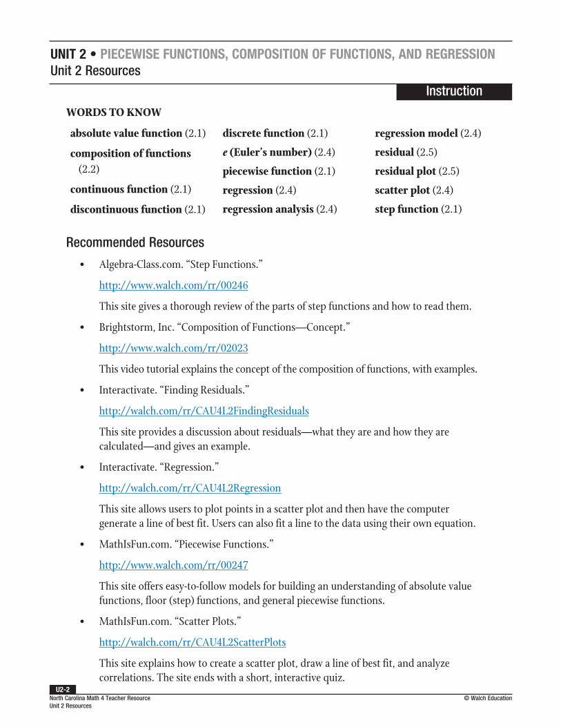
UNIT 2 • PIECEWISE FUNCTIONS, COMPOSITION OF FUNCTIONS, AND REGRESSIONUnit 2 Resources
Instruction
North Carolina Math 4 Teacher Resource Unit 2 Resources
© Walch Education
absolute value function (2.1)
composition of functions (2.2)
continuous function (2.1)
discontinuous function (2.1)
discrete function (2.1)
e (Euler’s number) (2.4)
piecewise function (2.1)
regression (2.4)
regression analysis (2.4)
regression model (2.4)
residual (2.5)
residual plot (2.5)
scatter plot (2.4)
step function (2.1)
WORDS TO KNOW
Recommended Resources
• Algebra-Class.com. “Step Functions.”
http://www.walch.com/rr/00246
This site gives a thorough review of the parts of step functions and how to read them.
• Brightstorm, Inc. “Composition of Functions—Concept.”
http://www.walch.com/rr/02023
This video tutorial explains the concept of the composition of functions, with examples.
• Interactivate. “Finding Residuals.”
http://walch.com/rr/CAU4L2FindingResiduals
This site provides a discussion about residuals—what they are and how they are calculated—and gives an example.
• Interactivate. “Regression.”
http://walch.com/rr/CAU4L2Regression
This site allows users to plot points in a scatter plot and then have the computer generate a line of best fit. Users can also fit a line to the data using their own equation.
• MathIsFun.com. “Piecewise Functions.”
http://www.walch.com/rr/00247
This site offers easy-to-follow models for building an understanding of absolute value functions, floor (step) functions, and general piecewise functions.
• MathIsFun.com. “Scatter Plots.”
http://walch.com/rr/CAU4L2ScatterPlots
This site explains how to create a scatter plot, draw a line of best fit, and analyze correlations. The site ends with a short, interactive quiz.
U2-2
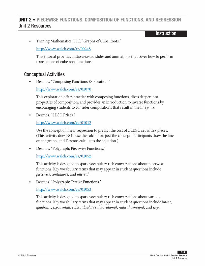
UNIT 2 • PIECEWISE FUNCTIONS, COMPOSITION OF FUNCTIONS, AND REGRESSIONUnit 2 Resources
Instruction
North Carolina Math 4 Teacher Resource Unit 2 Resources
© Walch Education
• Twining Mathematics, LLC. “Graphs of Cube Roots.”
http://www.walch.com/rr/00248
This tutorial provides audio-assisted slides and animations that cover how to perform translations of cube root functions.
Conceptual Activities• Desmos. “Composing Functions Exploration.”
http://www.walch.com/ca/01070
This exploration offers practice with composing functions, dives deeper into properties of composition, and provides an introduction to inverse functions by encouraging students to consider compositions that result in the line y = x.
• Desmos. “LEGO Prices.”
http://www.walch.com/ca/01012
Use the concept of linear regression to predict the cost of a LEGO set with x pieces. (This activity does NOT use the calculator, just the concept. Participants draw the line on the graph, and Desmos calculates the equation.)
• Desmos. “Polygraph: Piecewise Functions.”
http://www.walch.com/ca/01052
This activity is designed to spark vocabulary-rich conversations about piecewise functions. Key vocabulary terms that may appear in student questions include piecewise, continuous, and interval.
• Desmos. “Polygraph: Twelve Functions.”
http://www.walch.com/ca/01053
This activity is designed to spark vocabulary-rich conversations about various functions. Key vocabulary terms that may appear in student questions include linear, quadratic, exponential, cubic, absolute value, rational, radical, sinusoid, and step.
U2-3


UNIT 2 • PIECEWISE FUNCTIONS, COMPOSITION OF FUNCTIONS, AND REGRESSIONLesson 2.1: Piecewise, Step, and Absolute Value Functions
Name: Date:NC.M4.AF.4.1, NC.M4.AF.4.2
Warm-Up 2.1
A piece of electronic test equipment delivers a different output voltage depending on the magnitude
and polarity (positive or negative) of the input voltage. The output voltage is the dependent
variable f(x) and the input voltage is the independent variable. The function f(x) that models this
behavior is shown on the graph. The curved part of f(x) is defined by the quadratic function model
f x x x( )2
33
13
32= − + .
–10 –8 –6 –4 –2 2 4 6 8 10
x
10
8
6
4
2
0
–2
–4
–6
–8
–10
y
f(x)
f(x)f(x)
1. The function representing the curve in the first quadrant is given: f x x x( )2
33
13
32= − + . What
is the restricted domain of this function?
2. What function represents the ray in the second quadrant?
3. What is the restricted domain of this function?
4. What function represents the line segment that intersects the y-axis?
5. What is the restricted domain of this function?
Lesson 2.1: Piecewise, Step, and Absolute Value Functions
© Walch Education North Carolina Math 4 Teacher Resource 2.1
U2-5

UNIT 2 • PIECEWISE FUNCTIONS, COMPOSITION OF FUNCTIONS, AND REGRESSIONLesson 2.1: Piecewise, Step, and Absolute Value Functions
Instruction
NC.M4.AF.4.1, NC.M4.AF.4.2
Warm-Up 2.1 Debrief
1. The function representing the curve in the first quadrant is given: f x x x( )2
33
13
32= − + . What
is the restricted domain of this function?
Notice that the endpoint of the graph at x = 2 is an open circle, which means that the restricted
domain for his curve begins at but does not include x = 2. Therefore, the restricted domain of
f x x x( )2
33
13
32= − + is (2, )∞ .
2. What function represents the ray in the second quadrant?
The ray is part of a horizontal line. The general equation of a linear function in slope-intercept form is f(x) = mx + b, where m is the slope and b is the y-intercept. Since there is no change in the slope, the slope of the horizontal ray is 0. The y-intercept would be 4 if the line was extended to the y-axis. Therefore, substitute 0 for m and 4 for b into the general form, and simplify to determine the equation of the function.
f(x) = mx + b General form of a linear function in slope-intercept form
f(x) = (0)x + (4) Substitute 0 for m and 4 for b.
f(x) = 4 Simplify.
The function that represents the ray in the second quadrant is f(x) = 4.
3. What is the restricted domain of this function?
The open circle at x = –3 means “up to but not including” x = –3. Therefore, the restricted domain for f(x) = 4 is ( , 3)−∞ − .
Lesson 2.1: Piecewise, Step, and Absolute Value FunctionsNorth Carolina Math 4 Standards
NC.M4.AF.1.1 Execute algebraic procedures to compose two functions.
NC.M4.AF.1.2 Execute a procedure to determine the value of a composite function at a given value when the functions are in algebraic, graphical, or tabular representations.
© Walch EducationNorth Carolina Math 4 Teacher Resource 2.1
U2-6

UNIT 2 • PIECEWISE FUNCTIONS, COMPOSITION OF FUNCTIONS, AND REGRESSIONLesson 2.1: Piecewise, Step, and Absolute Value Functions
Instruction
NC.M4.AF.4.1, NC.M4.AF.4.2
4. What function represents the line segment that intersects the y-axis?
To determine the function for the line segment, first calculate the slope.
The slope of a line is given by the formula my y
x x2 1
2 1
=−−
. Substitute the two endpoints of the line
segment, (–3, 1) and (2, 5), into this formula and solve for m.
my y
x x2 1
2 1
=−− Slope formula
m(1) (5)
( 3) (2)=
−− −
Substitute 2 for x1, –3 for x2, 5 for y1, and 1 for y2.
m4
5= Simplify.
The slope of the line is m4
5= .
Though we could use the slope-intercept form to determine the function as in the answer to problem 1, it is difficult to precisely approximate the y-intercept from the graph. Therefore, to more accurately find the equation of the line, substitute either of the previously determined endpoints along with the slope into the point-slope formula, y – y1 = m(x – x1). Then, simplify the equation.
Let’s use the endpoint (2, 5).
y – y1 = m(x – x1) Point-slope formula
y x(5)4
5[ (2)]− =
− Substitute 4
5 for m, 2 for x1, and 5 for y1.
5(y – 5) = 4(x – 2) Multiply both sides by 5.
5y – 25 = 4x – 8 Distribute.
5y = 4x + 17 Add 25 to both sides.
y x4
5
17
5= + Divide both sides by 5.
The function that represents the line segment that intersects the y-axis is f x x( )4
5
17
5= + .
© Walch Education North Carolina Math 4 Teacher Resource 2.1
U2-7

UNIT 2 • PIECEWISE FUNCTIONS, COMPOSITION OF FUNCTIONS, AND REGRESSIONLesson 2.1: Piecewise, Step, and Absolute Value Functions
Instruction
NC.M4.AF.4.1, NC.M4.AF.4.2
5. What is the restricted domain of this function?
Notice that the endpoints are solid circles; this means that the x-values of –3 and 2 are included in the restricted domain. Therefore, the restricted domain is given by [–3, 2].
Connection to the Lesson
• Students will identify the restricted domains of a function from a graph of the function.
• Students will use formulas and rules to determine the algebraic form of a function using coordinates or data points of the function.
© Walch EducationNorth Carolina Math 4 Teacher Resource 2.1
U2-8

UNIT 2 • PIECEWISE FUNCTIONS, COMPOSITION OF FUNCTIONS, AND REGRESSIONLesson 2.1: Piecewise, Step, and Absolute Value Functions
Instruction
NC.M4.AF.4.1, NC.M4.AF.4.2
Introduction
Many real-world applications of mathematics involve the use of two or more functions to describe relationships among several variables. These functions sometimes apply to the problem over different domains that correspond to different real-world conditions. For example, a quadratic function model might describe a real-world relationship between two variables over the interval (a, b], but an exponential function model might better describe the relationship over the interval (b, c). In other words, portions of the same overall function can be defined by different equations over different domain intervals. The ability to apply a function model to a collection of data points depends, in part, on the ability to identify trends among data values and to associate those with an appropriate function type.
Key Concepts
• A piecewise function is a function that is defined by two or more expressions on separate portions of the domain.
• Such functions can be continuous, with no break in the graph of the function across a specified domain, or discontinuous, in which the graph of the function has a break, hole, or jump.
• A discrete function is a function in which every element of the domain is individually separate and distinct.
• Use a brace to show two (or more) pieces of the same function over different restricted domains. When stating the domain of the entire piecewise function, write the domain for each individual piece next to the appropriate expression. For example, for the piecewise function a(x):
a xx x
x x( )
4.57• ; 10
3.43• ; 10=
≤>
Prerequisite Skills
This lesson requires the use of the following skills:
• identifying restricted domains of parts of functions from observing a graph that has curves, line, and segments with open or solid endpoints of the graphs of those parts of functions (F–IF.5)
• using rules for calculating maximum or minimum points, slopes, x-intercepts, and y-intercepts to write equations for functions from the graphs of those functions (F–IF.4, F–LE.2)
© Walch Education North Carolina Math 4 Teacher Resource 2.1
U2-9

UNIT 2 • PIECEWISE FUNCTIONS, COMPOSITION OF FUNCTIONS, AND REGRESSIONLesson 2.1: Piecewise, Step, and Absolute Value Functions
Instruction
NC.M4.AF.4.1, NC.M4.AF.4.2
• One piece of the function, a(x) = 4.57 • x, represents the portion of the function over the restricted domain x ≤ 10. The other piece, a(x) = 3.43 • x, represents the portion of the function for which x > 10.
• An absolute value function is a function of the form f x ax b c( )= + + , where x is the independent variable and a, b, and c are real numbers. An absolute value function is a special type of piecewise function because the function values on either side of its maximum or minimum point are equal; for example, if f x x( ) 6= − , then f(3) = f(9). In general terms, an absolute value function can be represented by f x x a b( )= + + , where the maximum or minimum function value occurs at the point (–a, b).
• For a value of x = m in which m < a, or a value of x = m in which m > a, the function value f(m) is the same because the absolute value of the quantity a + m is the same under both conditions, namely a m b+ + .
• A step function (sometimes called a floor function or a postage function) is another special type of piecewise function that is discontinuous. A step function is a combination of one or more functions that are defined over restricted intervals and which may be undefined at other domain points or over other restricted domain intervals. In other words, a step function is a series of disconnected constant functions.
• A common type of step function is one in which the function values are restricted to integer domain values, such as the number of students who join the computer-gaming club—each student must be represented by a whole number (integer) value.
• By contrast, a function that models temperature changes throughout the day would not be restricted to integer domain values, since the temperature fluctuates by fractions of degrees.
• Just as with exponential, linear, and quadratic functions, domain and range variables for real-world problems involving piecewise functions may require adjustments to the axis scales when creating graphs and other visual aids.
Common Errors/Misconceptions
• applying a function model to a real-world problem without checking to see if the model’s features and solutions actually explain the problem’s data
• thinking of a piecewise function as a special type of step function rather than the other way around
• forgetting to check to see if the restricted domains of several functions making up a piecewise function together cover the complete domain of the piecewise function and its component parts
© Walch EducationNorth Carolina Math 4 Teacher Resource 2.1
U2-10

UNIT 2 • PIECEWISE FUNCTIONS, COMPOSITION OF FUNCTIONS, AND REGRESSIONLesson 2.1: Piecewise, Step, and Absolute Value Functions
Name: Date:NC.M4.AF.4.1, NC.M4.AF.4.2
© Walch Education North Carolina Math 4 Teacher Resource 2.1
U2-11
Problems 1–3 each describe a different function derived from the data in the table. Use the table to describe the pieces of the combined function and their domain intervals, and write the letters of the points contained within each interval.
A B C D Ex –2 –1 0 1 2y 0.0625 0.25 1 0.5 1
1. a piecewise function that is a combination of an exponential function and a linear function
2. a step function consisting of four steps of the forms y = a, y = b, y = c, and y = d
3. a piecewise function that is a combination of an absolute value function and a quadratic function
Use the graph of f(x), g(x), and h(x) to complete problems 4–6.
–10 –8 –6 –4 –2 2 4 6 8 10
x
10
8
6
4
2
0
–2
–4
–6
–8
–10
y
f(x)g(x)
h(x)
4. Name the two functions that are of the forms y a x b•= + and y a x•= .
5. Name the two functions that are of the forms y a x•= and y b x•= .
6. Name the two functions that are of the forms y a x b•= + and y b x•= .
continued
Scaffolded Practice 2.1: Piecewise, Step, and Absolute Value Functions

UNIT 2 • PIECEWISE FUNCTIONS, COMPOSITION OF FUNCTIONS, AND REGRESSIONLesson 2.1: Piecewise, Step, and Absolute Value Functions
Name: Date:NC.M4.AF.4.1, NC.M4.AF.4.2
© Walch EducationNorth Carolina Math 4 Teacher Resource 2.1
U2-12
For problems 7–10, identify whether the function model described is an absolute value inequality, a combination function, a piecewise function, or a step function.
7. a taxi’s fare is $5 plus $0.50 per quarter mile
8. a graduation test score that is within 20 points of the average class score
9. the constant terminal speed reached by a parachutist after free-falling (accelerating) for 30 seconds
10. the population of snapping turtles in a retention pond if the population increases annually at half the preceding year’s rate for 5 consecutive years, but has a maximum value due to the limited resources in the pond

UNIT 2 • PIECEWISE FUNCTIONS, COMPOSITION OF FUNCTIONS, AND REGRESSIONLesson 2.1: Piecewise, Step, and Absolute Value Functions
Instruction
NC.M4.AF.4.1, NC.M4.AF.4.2
Example 1
A wholesale store sells paper plates for $3.27 per package, up to and including 50 packages purchased. If a customer buys more than 50 packages, the price of the entire purchase drops to $2.73 per package. Write a piecewise function for this pricing structure, and determine the price a deli owner would pay for 75 packages of plates.
1. Write a function for the price paid for 50 or fewer packages of plates.
Let the total price be t, the price per package be p, and the number of packages be n. Thus, the total price, t, of n packages is t(n).
The general function t(n) = p • n represents the price paid for 50 or fewer packages of plates.
We are given that the price per package is $3.27, up to and including 50 packages purchased; therefore, let p = 3.27.
This function can be written as t(n) = 3.27 • n, if n ≤ 50.
2. Write a function for the price paid for more than 50 packages of plates.
Again, let the total price be t, the price per package be p, the number of packages be n, and the total price, t, of n packages be t(n).
Thus, the general function from step 1, t(n) = p • n, also represents the price paid for more than 50 packages of plates.
However, the given price per package for more than 50 packages is $2.73; therefore, let p = 2.73.
Substituting the new price of $2.73 for p, this function can be written as t(n) = 2.73 • n, if n > 50.
3. Combine the two functions to show the “pieces” of the piecewise function and the restricted domain for each.
Write the functions and restrictions for the two different pricing structures using appropriate notation.
t nn n
n n( )
3.27• ; 50
2.73• ; 50=
≤>
Guided Practice 2.1
© Walch Education North Carolina Math 4 Teacher Resource 2.1
U2-13

UNIT 2 • PIECEWISE FUNCTIONS, COMPOSITION OF FUNCTIONS, AND REGRESSIONLesson 2.1: Piecewise, Step, and Absolute Value Functions
Instruction
NC.M4.AF.4.1, NC.M4.AF.4.2
4. Calculate the price paid for 75 packages of plates.
The part of the piecewise function, t(n), that applies to n = 75 is t(n) = 2.73 • n. Therefore, the price for 75 packages of plates is t(75) = 2.73 • 75 or $204.75.
Example 2
When heat energy is added to ice that has a temperature less than the freezing point of water, the heat goes into raising the temperature of the ice until it starts to melt. When the ice starts to melt, all of the heat goes into melting the ice, not raising the temperature of the ice-water mixture. After the ice is melted, the heat goes back into raising the temperature of the water that results from the ice melting. The following graph shows these three distinct phenomena.
20 40 60 80 100 120 140 160
H
30
25
20
15
10
5
0
–5
–10
–15
–20
–25
–30
T
Heat in joules (in thousands)
Tem
pera
ture
(°C)
Ice
Ice-water mix
Water
In this situation, the heat energy is added to the ice in such a way that it can be described by a quadratic function model. The “ice-water mix” and “water” parts of the heat-temperature function and graph are linear functions. Use a graphing calculator to derive a function for each of the three parts of this piecewise function. Then, write the complete function and its domain.
© Walch EducationNorth Carolina Math 4 Teacher Resource 2.1
U2-14

UNIT 2 • PIECEWISE FUNCTIONS, COMPOSITION OF FUNCTIONS, AND REGRESSIONLesson 2.1: Piecewise, Step, and Absolute Value Functions
Instruction
NC.M4.AF.4.1, NC.M4.AF.4.2
1. Determine the values of the three data points for the “ice” part of the function.
Notice that the H or horizontal axis numbers have to be multiplied by 1,000 to yield the “true” values of x needed for finding the specific function equation. From the graph, it can be seen that the first point is at (0, –25). The second point appears to have an H-coordinate that is located at two thirds of the interval from 0 to 40 multiplied by 1,000. Two thirds of 40,000 is approximately 26,667. The T-coordinate of this point is –20; therefore, the second point is at approximately (26,667, –20). The third point has an H-coordinate of 40 times 1,000, so the third point’s coordinates are (40,000, 0).
The locations of the three data points can be approximated as (0, –25), (26,667, –20), and (40,000, 0).
2. Use the three data points for the “ice” part of the function to find the equation of the quadratic function.
Use a graphing calculator to determine the equation of this part of the function. Follow the directions appropriate to your calculator model.
On a TI-83/84:
Step 1: Press [STAT] to bring up the statistics menu. The first option, 1: Edit, will already be highlighted. Press [ENTER].
Step 2: Arrow up to L1 and press [CLEAR], then [ENTER], to clear the list. Repeat this process to clear L2 and L3 if needed.
Step 3: Enter the three ordered pairs from example step 1 in the L1 and L2 lists. Make sure to enter the H-coordinates in L1 and the T-coordinates in L2.
Step 4: Press [STAT]. Arrow to the CALC menu. Select 5: QuadReg.
Step 5: Press [2ND][1] to type “L1” for Xlist. Arrow down to Ylist and press [2ND][2] to type “L2” for Ylist, if not already shown.
Step 6: Arrow down to “Calculate” and press [ENTER].(continued)
© Walch Education North Carolina Math 4 Teacher Resource 2.1
U2-15

UNIT 2 • PIECEWISE FUNCTIONS, COMPOSITION OF FUNCTIONS, AND REGRESSIONLesson 2.1: Piecewise, Step, and Absolute Value Functions
Instruction
NC.M4.AF.4.1, NC.M4.AF.4.2
On a TI-Nspire:
Step 1: Press [home]. Arrow over to the spreadsheet icon, the fourth icon from the left, and press [enter].
Step 2: To clear the lists in your calculator, arrow up to the topmost cell of the table to highlight the entire column, then press [menu]. Choose 3: Data, then 4: Clear Data. Repeat for each column as necessary.
Step 3: Arrow up to the topmost cell of the first column, labeled “A.” Press [X][enter] to type x. Then, arrow over to the second column, labeled “B.” Press [Y][enter] to type y.
Step 4: Arrow down to cell A1 and enter the first H-value from the ordered pairs in example step 1. Press [enter]. Enter the second H-value in cell A2 and so on.
Step 5: Move over to cell B1 and enter the first T-value. Press [enter]. Enter the second T-value in cell B2 and so on.
Step 6: To fit an equation to the data points, press [menu] and select 4: Statistics, then 1: Stat Calculations, then 6: Quadratic Regression. Select “x” from the X List pop-up menu. Press [tab] to move to the Y List pop-up menu, then select “y” from the options. Tab to “OK” and press [enter].
Either calculator will return values for the constants that can be substituted into the equation y = ax2 + bx + c.
The result is the quadratic equation y = (3.28135 • 10–8)x2 + (–6.875 • 10–4)x – 25.
3. Rewrite the resulting equation as a function using the variables H and T, and list the restricted domain over which the function is defined.
The equation generated by the calculator for the “ice” part of the function can be written as shown:
T(H) = (3.28135 • 10–8)H2 + (–6.875 • 10–4)H – 25
From the graph, it can be seen that the domain for this function is [0, 40,000].
© Walch EducationNorth Carolina Math 4 Teacher Resource 2.1
U2-16

UNIT 2 • PIECEWISE FUNCTIONS, COMPOSITION OF FUNCTIONS, AND REGRESSIONLesson 2.1: Piecewise, Step, and Absolute Value Functions
Instruction
NC.M4.AF.4.1, NC.M4.AF.4.2
4. Write the equation for the “ice-water mix” part of the piecewise function, and list the restricted domain over which the function is defined.
The ice-water mix is a horizontal line with a slope of 0 that would intersect the y-axis at 0. Therefore, the equation for this piece of the function can be written as T(H) = 0.
An additional point appears to have an H-coordinate that is located at one-third of the interval from 120 to 160 multiplied by 1,000. One-third of 40,000 is approximately 13,333, so 120,000 + 13,333 is 133,333. The T-coordinate of this point is 0; therefore, the additional data point is at approximately (133,333, 0).
From the graph, it can be seen that the domain for this function is approximately [40,000, 133,333].
5. Write the two points defining the “water” part of the function graph.
From the graph, it can be seen that one point is (120,000, 0) and the other is (140,000, 30).
6. Write the equation for the “water” part of the function.
First, calculate the slope of the line using the formula for slope,
my y
x x2 1
2 1
=−−
. Substitute the points determined from the previous step,
(140,000, 30) and (120,000, 0), and then solve for the slope, m.
my y
x x2 1
2 1
=−− Slope formula
m(0) (30)
(120,000) (140,000)=
−−
Substitute 140,000 for x1, 120,000 for x2, 30 for y1, and 0 for y2.
m30
20,000=
−−
Simplify.
m = 1.5 • 10–3
The slope of the line is m = 0.0015 • 0.001.(continued)
© Walch Education North Carolina Math 4 Teacher Resource 2.1
U2-17

UNIT 2 • PIECEWISE FUNCTIONS, COMPOSITION OF FUNCTIONS, AND REGRESSIONLesson 2.1: Piecewise, Step, and Absolute Value Functions
Instruction
NC.M4.AF.4.1, NC.M4.AF.4.2
Use the point-slope formula, y – y1 = m(x – x1), along with the slope and either of the two points from the previous step to write the equation for the “water” part of the function.
Let’s use (120,000, 0).
y – y1 = m(x – x1) Point-slope formula
y – (0) = (0.0015 • 0.001)[x – (120,000)]
Substitute 120,000 for x1, 0 for y1, and 0.0015 • 0.001 for m.
y = (0.0015 • 0.001)x – 180 Simplify.
The equation for the “water” part of the function is y = (0.0015 • 0.001)x – 180.
7. Rewrite the resulting equation as a function using the variables H and T, and list the restricted domain over which the function is defined.
The equation can be written as T(H) = 0.0015H – 180.
From the graph, it can be seen that the domain for this function is [120,000, 140,000].
8. Write the complete piecewise function for T(H), and determine its domain.
T H
H H H
H
H H
( )
(3.28135•10 ) ( 6.875•10 ) 25; 0 40,000
0; 40,000 120,000
0.0015 180; 120,000 140,000
8 2 4
( )=
+ − − ≤ ≤< <− ≤ ≤
− −
Comparing the three pieces of the function and their restricted domains, the lowest domain value is 0, and the highest is 140,000. Both are included, as shown by the ≤ symbols. Therefore, the domain for the piecewise function T(H) is [0, 140,000].
© Walch EducationNorth Carolina Math 4 Teacher Resource 2.1
U2-18

UNIT 2 • PIECEWISE FUNCTIONS, COMPOSITION OF FUNCTIONS, AND REGRESSIONLesson 2.1: Piecewise, Step, and Absolute Value Functions
Instruction
NC.M4.AF.4.1, NC.M4.AF.4.2
Example 3
The graph shows a quadratic step function, f x x x( )3
42
7
42= − − . What domain restriction defines each
step? Use the graph to write the equations of the steps of the quadratic function, and determine each
step’s restricted domain. Then, use this information to determine the domain of the quadratic function.
–10 –8 –6 –4 –2 2 4 6 8 10
x
10
8
6
4
2
0
–2
–4
–6
–8
–10
y
1. Write an equation of the form y = a for each of the three function steps shown.
The step equations are y = 1 (Quadrant II), y = –3 (Quadrants III and IV), and y = –1 (Quadrant IV).
2. Write the restricted domain for each equation.
For y = 1, there is a closed circle at x = –1 and an open circle at x = –3. Therefore, the domain of y = 1 is (–3, –1].
For y = –1, there is an open circle at x = 1 and a closed circle at x = 3. Therefore, the domain of y = –1 is (1, 3].
For y = –3, there is an open circle at x = –1 and a closed circle at x = 1. Therefore, the domain of y = –3 is (–1, 1].
© Walch Education North Carolina Math 4 Teacher Resource 2.1
U2-19

UNIT 2 • PIECEWISE FUNCTIONS, COMPOSITION OF FUNCTIONS, AND REGRESSIONLesson 2.1: Piecewise, Step, and Absolute Value Functions
Instruction
NC.M4.AF.4.1, NC.M4.AF.4.2
3. Use the restricted domains of the step functions to determine the rule that defines the domain of the quadratic function f(x).
The value of the quadratic function is given by the upper bound or limit of the interval over which each step is defined. Therefore, the domain of f(x) is defined by the rule {x = –1, 1, and 3}.
4. Write the full function f(x) along with the domain of the quadratic function.
Use the pieces of the function, the given quadratic function, and each of the domains to write the step function f(x).
f x
x x x
x
x
x
( )
3
42
7
4; 1,1,3
1; 3 1
3; 1 1
1;1 3
2
=
− − =−
− < ≤−− − < ≤− < ≤
© Walch EducationNorth Carolina Math 4 Teacher Resource 2.1
U2-20

UNIT 2 • PIECEWISE FUNCTIONS, COMPOSITION OF FUNCTIONS, AND REGRESSIONLesson 2.1: Piecewise, Step, and Absolute Value Functions
Instruction
NC.M4.AF.4.1, NC.M4.AF.4.2
Example 4
Use a graphing calculator to compare the graphs of the three functions f x x x( ) 3= + − , g(x) = 2x – 3, and h(x) = –2x + 3. How are the functions related? How are they alike and different?
1. Graph the functions using a graphing calculator.
Enter each function into your graphing calculator. Graph all three functions on the same coordinate plane.
–10 –8 –6 –4 –2 2 4 6 8 10
x
10
8
6
4
2
0
–2
–4
–6
–8
–10
y
f(x) = |x| + |x – 3|
g(x) = 2x – 3 h(x) = –2x + 3
2. Describe the equations and domains of the three pieces of the piecewise function f(x).
Refer to the graph and the given equations.
The piecewise function f(x) has one piece that is defined by the rule f(x) = –2x + 3 for the restricted domain ,0( )−∞ , another that is defined by the rule f(x) = 3 for the restricted domain [0, 3], and a third that is defined by the rule f(x) = 2x – 3 for the restricted domain 3,( )∞ . All three rules comprise f(x).
© Walch Education North Carolina Math 4 Teacher Resource 2.1
U2-21

UNIT 2 • PIECEWISE FUNCTIONS, COMPOSITION OF FUNCTIONS, AND REGRESSIONLesson 2.1: Piecewise, Step, and Absolute Value Functions
Instruction
NC.M4.AF.4.1, NC.M4.AF.4.2
3. Describe what the function y = 3 represents for f(x).
The minimum function value is 3, which occurs over the restricted domain [0, 3]. Therefore, y = 3 represents the minimum, or lowest value, of the function f(x).
4. Determine the intersection point of the graphs of g(x) and h(x), and describe what it represents.
Based on the graph of the functions, the intersection point is (1.5, 0). This point represents the domain value at which the function values are equal.
5. Describe the meaning of the overlapping portions of the graphs of the function pair f(x) and g(x) as well as the function pair f(x) and h(x).
The overlap means that the function pairs share the same points for those domain values. It also means that the overlapping domains are solutions for the pairs of functions.
6. Determine the solutions for the function pair f(x) and g(x) and the function pair f(x) and h(x).
Based on the graphs and the overlapping domains, the solution set for f(x) and g(x) is given by the domain interval 3,[ )∞ . The solution set for f(x) and h(x) is given by the domain interval ,0](−∞ .
© Walch EducationNorth Carolina Math 4 Teacher Resource 2.1
U2-22

UNIT 2 • PIECEWISE FUNCTIONS, COMPOSITION OF FUNCTIONS, AND REGRESSIONLesson 2.1: Piecewise, Step, and Absolute Value Functions
Name: Date:NC.M4.AF.4.1, NC.M4.AF.4.2
Problem-Based Task 2.1: Motorcycle Engine Tolerances
Aliza is a mechanical engineer who designs motorcycle engines. She uses a mathematical model to maximize the combustion and compression efficiency of each engine she designs. Since the piston of the latest engine Aliza designed will be manufactured at a different factory from the combustion chamber into which it fits, there will be small but significant variations in the radii of the pistons and the combustion chambers. An absolute-value function, called the tolerance ratio, compares the amount of allowable variation, r, in the radius of the piston to the amount of allowable variation in the radius of the combustion chamber. These allowable variations are equal for all practical purposes, but are accounted for in Aliza’s function model. (Note: r is in millimeters.)
Aliza has decided that the tolerance ratio for the new engine has to be less than 0.9 in order for the
engine to meet quality expectations. Use the tolerance ratio function, T rr
r( )
0.001
0.002=
−+
, to write an
absolute value inequality with the given tolerance-ratio condition for this engine. Then, calculate the
range of values of r that meet the criteria.
SMP 1 ✓ 2 ✓3 ✓ 4 ✓5 ✓ 6 ✓7 ✓ 8 ✓
Use the tolerance ratio function to write an absolute value inequality with the given tolerance-ratio condition for this engine.
© Walch Education North Carolina Math 4 Teacher Resource 2.1
U2-23
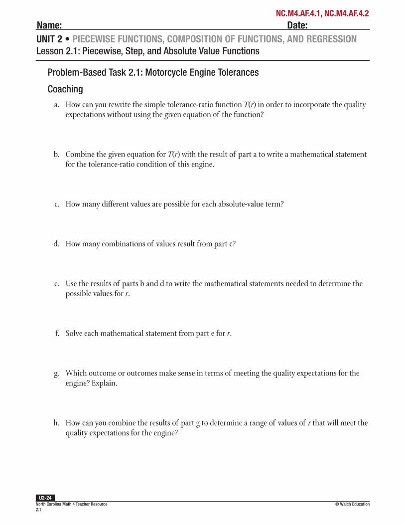
UNIT 2 • PIECEWISE FUNCTIONS, COMPOSITION OF FUNCTIONS, AND REGRESSIONLesson 2.1: Piecewise, Step, and Absolute Value Functions
Name: Date:NC.M4.AF.4.1, NC.M4.AF.4.2
Problem-Based Task 2.1: Motorcycle Engine Tolerances
Coaching
a. How can you rewrite the simple tolerance-ratio function T(r) in order to incorporate the quality expectations without using the given equation of the function?
b. Combine the given equation for T(r) with the result of part a to write a mathematical statement for the tolerance-ratio condition of this engine.
c. How many different values are possible for each absolute-value term?
d. How many combinations of values result from part c?
e. Use the results of parts b and d to write the mathematical statements needed to determine the possible values for r.
f. Solve each mathematical statement from part e for r.
g. Which outcome or outcomes make sense in terms of meeting the quality expectations for the engine? Explain.
h. How can you combine the results of part g to determine a range of values of r that will meet the quality expectations for the engine?
© Walch EducationNorth Carolina Math 4 Teacher Resource 2.1
U2-24

UNIT 2 • PIECEWISE FUNCTIONS, COMPOSITION OF FUNCTIONS, AND REGRESSIONLesson 2.1: Piecewise, Step, and Absolute Value Functions
Instruction
NC.M4.AF.4.1, NC.M4.AF.4.2
Problem-Based Task 2.1: Motorcycle Engine Tolerances
Coaching Sample Responses
a. How can you rewrite the simple tolerance-ratio function T(r) in order to incorporate the quality expectations without using the given equation of the function?
The tolerance ratio has to be less than 0.9 in order for the engine to meet its quality expectations. Therefore, the simple tolerance ratio function can be written as T(r) < 0.9.
b. Combine the given equation for T(r) with the result of part a to write a mathematical statement for the tolerance-ratio condition of this engine.
Since T(r) in the tolerance-ratio equation T rr
r( )
0.001
0.002=
−+
must be less than 0.9 for this engine,
the mathematical statement for this condition is r
r
0.001
0.0020.9
−+
< .
c. How many different values are possible for each absolute-value term?
Each absolute-value term can be positive or negative; also, the absolute-value quantity in the numerator could be 0, but the quantity in the denominator cannot if the function is to exist.
d. How many combinations of values result from part c?
There are four possibilities:
For the numerator: r – 0.001 > 0 or r – 0.001 < 0
For the denominator: r + 0.002 > 0 or r + 0.002 < 0
The numerator can also be written as r r0.001 0.001− = − or 0.001 – r, and the denominator can be written as r r0.002 0.002+ = + or –r – 0.002.
© Walch Education North Carolina Math 4 Teacher Resource 2.1
U2-25

UNIT 2 • PIECEWISE FUNCTIONS, COMPOSITION OF FUNCTIONS, AND REGRESSIONLesson 2.1: Piecewise, Step, and Absolute Value Functions
Instruction
NC.M4.AF.4.1, NC.M4.AF.4.2
e. Use the results of parts b and d to write the mathematical statements needed to determine the possible values for r.
Create a table using the four cases from part d to efficiently organize the results.
|r – 0.001| |r – 0.002| Function ratio Simplified statement
> 0 > 0r
r
0.001
0.0020.9
−+
< r – 0.001 < 0.9(r + 0.002)
> 0 < 0r
r
0.001
0.0020.9
−− −
< r – 0.001 < 0.9(–r – 0.002)
< 0 < 0r
r
0.001
0.0020.9
− +− −
< 0.001 – r < 0.9(–r – 0.002)
< 0 > 0r
r
0.001
0.0020.9
− ++
< 0.001 – r < 0.9(r + 0.002)
f. Solve each mathematical statement from part e for r.
For r – 0.001 < 0.9(r + 0.002), the value is r < 0.028 mm.
For r – 0.001 < 0.9(–r – 0.002), the value is r < –0.000421 mm.
For 0.001 – r < 0.9(–r – 0.002), the value is r > 0.028 mm.
For 0.001 – r < 0.9(r + 0.002), the value is r > –0.000421 mm.
g. Which outcome or outcomes make sense in terms of meeting the quality expectations for the engine? Explain.
Alone, none of the answers makes physical sense, because each implies an open-ended domain of r-values: ,0.028( )−∞ , , 0.000421( )−∞ − , 0.028,( )∞ , and 0.000421,( )− ∞ . However, by combining the results, domains can be produced that do make physical sense.
h. How can you combine the results of part g to determine a range of values of r that will meet the quality expectations for the engine?
The restricted domains can be combined to determine a range of r-values expressed by the compound inequality –0.000421 mm < r < 0.028 mm. Remember that r is the range of variation in the radius of the piston or combustion chamber that will meet the engine’s tolerance-ratio criteria, expressed by T(r) < 0.9. It is not the actual radius of the piston or combustion chamber.
Recommended Closure Activity
Select one or more of the essential questions for a class discussion or as a journal entry prompt.
© Walch EducationNorth Carolina Math 4 Teacher Resource 2.1
U2-26

UNIT 2 • PIECEWISE FUNCTIONS, COMPOSITION OF FUNCTIONS, AND REGRESSIONLesson 2.1: Piecewise, Step, and Absolute Value Functions
Name: Date:NC.M4.AF.4.1, NC.M4.AF.4.2
© Walch Education North Carolina Math 4 Teacher Resource 2.1
U2-27
The graph shows the temperature change that occurs when water is heated and changes from a liquid to a gas (steam), where temperature is T and heat is H. Notice that the vertical T-axis begins at 40°C, which is the initial temperature of the water. Use the graph to complete problems 1–4.
10 2 3 4 5 6 7 8
H
160
140
120
100
80
60
40
T
Heat (� 105 joules)
Tem
pera
ture
(°C
)
Water
Steam
Water Steam
1. Describe the pieces of this piecewise function.
2. Derive the temperature function T(H) for the heat domain interval when the water temperature rises from 40°C to 100°C.
3. Determine the equation for the heat domain values for T = 100°C.
4. Derive the temperature function T(H) for the heat domain interval when the water temperature rises above 100°C.
Practice 2.1: Piecewise, Step, and Absolute Value Functions
continued
A

UNIT 2 • PIECEWISE FUNCTIONS, COMPOSITION OF FUNCTIONS, AND REGRESSIONLesson 2.1: Piecewise, Step, and Absolute Value Functions
Name: Date:NC.M4.AF.4.1, NC.M4.AF.4.2
© Walch EducationNorth Carolina Math 4 Teacher Resource 2.1
U2-28
A square wave is a type of periodic wave function whose amplitude changes suddenly instead of gradually (like a sine wave does), resulting in a “square” graph instead of smooth curves. The data in the table represent the output voltage of a square wave used for switching an electric circuit off and on automatically. The function model V(t) represents the voltage, and time t is the independent variable. Dashes represent values of t for which the function is undefined. Use this information and the table to complete problems 5–7.
t 08
π4
π 3
8
π2
π 5
8
π 3
4
ππ
V(t) — 4 4 4 — –4 –4 –4
5. Explain how the results in the table imply that the function model is a step function.
6. The output voltage is periodic. What is its period?
7. The function that generated the values in the table is V tt
t( )
4• sin 2
sin 2= . Show how this function
could generate the table function values.
continued

UNIT 2 • PIECEWISE FUNCTIONS, COMPOSITION OF FUNCTIONS, AND REGRESSIONLesson 2.1: Piecewise, Step, and Absolute Value Functions
Name: Date:NC.M4.AF.4.1, NC.M4.AF.4.2
© Walch Education North Carolina Math 4 Teacher Resource 2.1
U2-29
The graph shows how the efficiency of an audio speaker varies with sound intensity. Efficiency is the speaker’s ability to transform power into sound. Use the graph and the information that follows to complete problems 8–10.
–10 –8 –6 –4 –2 2 4 6 8 10
i
10
8
6
4
2
0
–2
–4
–6
–8
–10
y
B(i) = 2 log (i + 1)
= i – 1i + 1
A(i)
The vertical asymptote i = –1 describes the intensity at which the ideal efficiency of the speaker for its designed frequency range is achieved. The functions shown represent models for how the efficiencies A(i) and B(i) vary at intensities above and below the efficiency ideal at i = –1. The function A(i) applies to the intensity interval ( , 1)−∞ − and models the efficiency of the speaker for very loud sounds. The function B(i) applies to the intensity interval P x x( ) 2 1= + and models the efficiency of the speaker for very faint sounds. (Note: The “efficiency” is a dimensionless number that is related to a variety of design and engineering factors that can have large positive and negative values for highly efficient speakers over a variety of frequency and power input-output ranges.)
8. How does A(i) change as the intensity approaches –1?
9. How does B(i) change as the intensity approaches –1?
10. How do the values of both functions change as the intensity changes from about –100 to about –1 and from about –1 to about 100?

UNIT 2 • PIECEWISE FUNCTIONS, COMPOSITION OF FUNCTIONS, AND REGRESSIONLesson 2.1: Piecewise, Step, and Absolute Value Functions
Name: Date:NC.M4.AF.4.1, NC.M4.AF.4.2
© Walch EducationNorth Carolina Math 4 Teacher Resource 2.1
U2-30
B
continued
Practice 2.1: Piecewise, Step, and Absolute Value Functions
The following graph is called a phase diagram. It shows the pressure and temperature at which a substance is a gas, a liquid, a solid, or all three phases of matter. The pressure scale, P(T), is in thousands, and the temperature scale T is in degrees Celsius. Use the graph to complete problems 1–4.
20 40 60 80 100 120
T
550
500
450
400
350
300
250
200
150
100
50
0
P(T)
A
B
C
D
E
F
Temperature (°C)
Pres
sure
(in
thou
sand
s)
Gas
Solid
Liquid
1. Why is the whole graph not a combination or piecewise function?
2. Which points could be used to define individual functions from the data on the graph? Determine the coordinates of those points.
3. What are the coordinates of the point on the graph at which all three phases of the substance exist?
4. What function type(s) can be used to model these data points?

UNIT 2 • PIECEWISE FUNCTIONS, COMPOSITION OF FUNCTIONS, AND REGRESSIONLesson 2.1: Piecewise, Step, and Absolute Value Functions
Name: Date:NC.M4.AF.4.1, NC.M4.AF.4.2
© Walch Education North Carolina Math 4 Teacher Resource 2.1
U2-31
Use the table to complete problems 5–7.
x –3 –2 –1 0 1 2 3f(x) 10 7 4 3 2 5 8
5. What type of function (linear, exponential, etc.) is represented by the data? Describe the evidence to support your answer, and determine the restricted intervals over which each function piece is defined.
6. The function represented by the data in the table has the general form f x x a b x a( ) •= + + − . Find the value of a.
7. Use the result of problem 6 to find the value of b. Be sure to check the values of a and b in each of the three restricted domains of the function.
continued
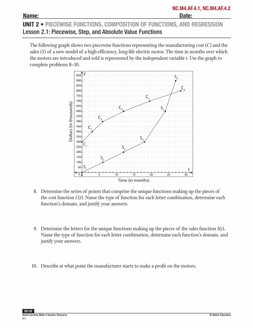
UNIT 2 • PIECEWISE FUNCTIONS, COMPOSITION OF FUNCTIONS, AND REGRESSIONLesson 2.1: Piecewise, Step, and Absolute Value Functions
Name: Date:NC.M4.AF.4.1, NC.M4.AF.4.2
© Walch EducationNorth Carolina Math 4 Teacher Resource 2.1
U2-32
The following graph shows two piecewise functions representing the manufacturing cost (C) and the sales (S) of a new model of a high-efficiency, long-life electric motor. The time in months over which the motors are introduced and sold is represented by the independent variable t. Use the graph to complete problems 8–10.
5 10 15 20 25 30
t
950
900
850
800
750
700
650
600
550
500
450
400
350
300
250
200
150
100
50
0
y
Time (in months)
Dol
lars
(in
thou
sand
s)
S1
C1
S2
S3
S4
S5
S6
C2
C3
C4
C5
C6
8. Determine the series of points that comprise the unique functions making up the pieces of the cost function C(t). Name the type of function for each letter combination, determine each function’s domain, and justify your answers.
9. Determine the letters for the unique functions making up the pieces of the sales function S(t). Name the type of function for each letter combination, determine each function’s domain, and justify your answers.
10. Describe at what point the manufacturer starts to make a profit on the motors.
Lesson 2.2: Composition of Functions
Warm-Up 2.2
Monica is an artist who makes stained glass lamps and sells them online. The function f(x) = 45x + 20 models her cost in dollars to create x lamps. The first 10 lamps she sells are priced at $120 each, but after she sells the first 10, she lowers the price to $100 to try to increase her sales.
1. Write a function g(x) to represent Monica’s income from selling the lamps.
2. Monica’s profit is determined by subtracting her costs from her income. Write a profit function P(x) in terms of f(x) and g(x).
3. Rewrite the profit function from problem 2 in terms of x, and use this function to determine Monica’s profit if she sells a total 24 lamps.
North Carolina Math 4 Teacher Resource 2.2
© Walch EducationU2-33
Name: Date:UNIT 2 • PIECEWISE FUNCTIONS, COMPOSITION OF FUNCTIONS, AND REGRESSIONLesson 2.2: Composition of Functions
NC.M4.AF.1.1

Warm-Up 2.2 Debrief
1. Write a function g(x) to represent Monica’s income from selling the lamps.
Monica sells the first 10 lamps for $120 each, which is a total of $1,200. Then she lowers the price to $100, so all lamps after the first 10 are priced at $100. If 10 lamps are sold for $120, then (x – 10) lamps are sold for $100.
Her income from selling lamps can be represented by the function g(x) = 1200 + 100(x – 10). This function can be simplified to g(x) = 200 + 100x, or in standard form, g(x) = 100x + 200.
2. Monica’s profit is determined by subtracting her costs from her income. Write a profit function P(x) in terms of f(x) and g(x).
In terms of cost f(x) and income g(x), Monica’s profit can be expressed as income minus cost: P(x) = g(x) – f(x).
3. Rewrite the profit function from problem 2 in terms of x, and use this function to determine Monica’s profit if she sells a total 24 lamps.
The function for cost is f(x) = 45x + 20 and the function for income is g(x) = 100x + 200. Substitute the expressions for f(x) and g(x) into the function for profit.
P(x) = g(x) – f(x) Profit function
P(x) = (100x + 200) – (45x + 20)Substitute (100x + 200) for g(x) and (45x + 20) for f(x).
P(x) = 100x + 200 – 45x – 20 Simplify.
P(x) = 55x + 180 Combine like terms.
The function that represents Monica’s profit is P(x) = 55x + 180. To calculate her profit for the sale of 24 lamps, substitute 24 for x in the profit function.
P(x) = 55x + 180 Profit function
P(x) = 55(24) + 180 Substitute 24 for x.
P(x) = 1500 Simplify.
If Monica sells 24 lamps online, she will earn a profit of $1,500.
Lesson 2.2: Composition of Functions
North Carolina Math 4 Standard
NC.M4.AF.1.1 Execute algebraic procedures to compose two functions.
North Carolina Math 4 Teacher Resource 2.2
© Walch EducationU2-34
UNIT 2 • PIECEWISE FUNCTIONS, COMPOSITION OF FUNCTIONS, AND REGRESSIONLesson 2.2: Composition of Functions
Instruction
NC.M4.AF.1.1
Connection to the Lesson
• Students apply the conditions of a real-world problem to the parts of an equation or function that models the problem.
• Students see one equation or function substituted into another equation or function and the effect that this substitution has on the variables in the model for the problem.
North Carolina Math 4 Teacher Resource 2.2
© Walch EducationU2-35
UNIT 2 • PIECEWISE FUNCTIONS, COMPOSITION OF FUNCTIONS, AND REGRESSIONLesson 2.2: Composition of Functions
Instruction
NC.M4.AF.1.1

North Carolina Math 4 Teacher Resource 2.2
© Walch EducationU2-36
UNIT 2 • PIECEWISE FUNCTIONS, COMPOSITION OF FUNCTIONS, AND REGRESSIONLesson 2.2: Composition of Functions
Instruction
Prerequisite Skills
This lesson requires the use of the following skills:
• translating real-world descriptions in a problem to mathematical terms (6.EE.6)
• substituting one expression for another in a mathematical statement (6.EE.2)
• checking a mathematical statement for accuracy and revising the statement when errors are found (6.EE.4)
Introduction
As you’ve seen, functions can be combined through addition, subtraction, multiplication, or division to produce a new function. Another way to combine functions is by using composition. The composition of two functions is done by substituting one function into the other function, thereby creating a new function. Compositions of functions are useful in modeling many types of problems.
Key Concepts
• The composition of functions is the process of substituting one function for the independent variable of another function to create a new function.
• The notation f(g(x)) or ( )( )f g x means that the function g(x) is substituted for the independent variable x in the function f(x). Similarly, the notation g(f(x)) or ( )( )g f x means that the function f(x) is substituted for the independent variable x in the function g(x).
• The domain and range of a function resulting from the composition of two functions should be compared to the domain and range of each of the functions used in the composition; the domain and range of the new function may not be the same as in the original functions.
Common Errors/Misconceptions
• substituting the wrong function into a second function during a composition of functions
• assuming that the domain and range of a function resulting from a composition will be the same as the domain and range of the functions that are composed
NC.M4.AF.1.1

Complete problems 1–8 as directed.
1. Rewrite f g x( )( ) using a different notation.
2. Rewrite g(f(x)) using a different notation.
3. Find f g x( )( ) if f x x( ) 1= − and g x x( ) = .
4. Find g f x( )( ) if f x x( ) 1= − and g x x( ) = .
5. Find f g x( )( ) if f x x( ) = and g x x( ) 2 1= + .
continued
Scaffolded Practice 2.2: Composition of Functions
North Carolina Math 4 Teacher Resource 2.2
© Walch EducationU2-37
Name: Date:UNIT 2 • PIECEWISE FUNCTIONS, COMPOSITION OF FUNCTIONS, AND REGRESSIONLesson 2.2: Composition of Functions
NC.M4.AF.1.1
6. Find g f x( )( ) if f x x( ) = and g x x( ) 2 1= + .
7. Find g f x( )( ) if g x x( ) 3= and f x x( ) 12= + .
8. Find f g x( )( ) if g x x( ) 3= and f x x( ) 12= + .
Use the functions f x x( ) 2= − and g x x( ) 1= − to complete problems 9–10.
9. What is f g x( )( ) ?
10. What is the domain of f g x( )( ) ?
North Carolina Math 4 Teacher Resource 2.2
© Walch EducationU2-38
Name: Date:UNIT 2 • PIECEWISE FUNCTIONS, COMPOSITION OF FUNCTIONS, AND REGRESSIONLesson 2.2: Composition of Functions
NC.M4.AF.1.1

Guided Practice 2.2
Example 1
Find the function that results from the composition f g x( )( ) if =−
f xx
( )1
3 and =
+g x
x( )
3
5.
Determine the domains of f(x), g(x), and f g x( )( ) .
1. To find f g x( )( ) , find f(g(x)).
Set f g x( )( ) equal to f(g(x)): =f g x f g x( )( ) ( ( )) . Then, substitute the expressions for f(x) and g(x) into the equation and simplify to find an expression for f g x( )( ) .
=f g x f g x( )( ) ( ( )) Composition rule
=+
f g x fx
( )( )3
5
Substitute +x
3
5 for g(x).
=
+
−
f g x
x
( )( )1
3
53
Substitute +x
3
5 for x in
the function f(x). (Recall
that =−
f xx
( )1
3.)
= − ++
f g x x
x
( )( )1
3 3( 5)
5
Combine the terms in the denominator.
= − −+
f g x x
x
( )( )1
3 12
5
Simplify the denominator.
=+
− −f g x
x
x( )( )
5
3 12
Simplify.
=+
− +f g x
x
x( )( )
5
3( 4) Factor the denominator.
The composition function is =+
− +f g x
x
x( )( )
5
3( 4) .
North Carolina Math 4 Teacher Resource 2.2
© Walch EducationU2-39
UNIT 2 • PIECEWISE FUNCTIONS, COMPOSITION OF FUNCTIONS, AND REGRESSIONLesson 2.2: Composition of Functions
Instruction
NC.M4.AF.1.1
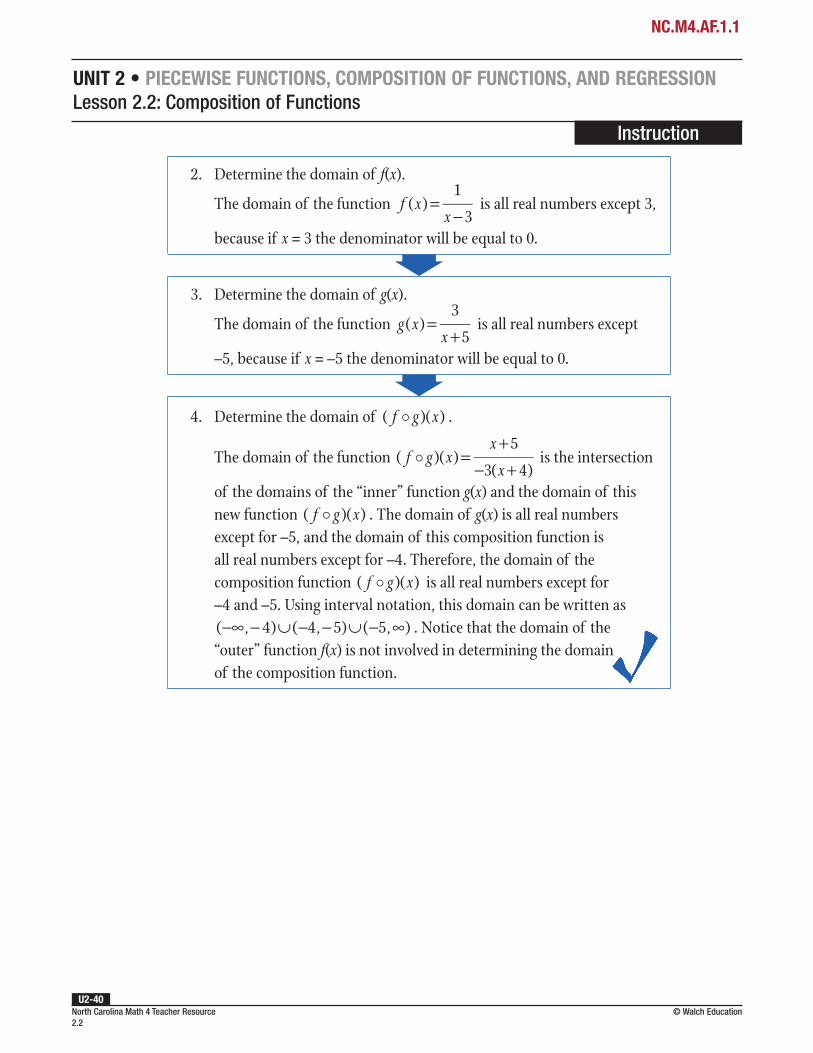
2. Determine the domain of f(x).
The domain of the function =−
f xx
( )1
3 is all real numbers except 3,
because if x = 3 the denominator will be equal to 0.
3. Determine the domain of g(x).
The domain of the function =+
g xx
( )3
5 is all real numbers except
–5, because if x = –5 the denominator will be equal to 0.
4. Determine the domain of f g x( )( ) .
The domain of the function =+
− +f g x
x
x( )( )
5
3( 4) is the intersection
of the domains of the “inner” function g(x) and the domain of this new function f g x( )( ) . The domain of g(x) is all real numbers except for –5, and the domain of this composition function is all real numbers except for –4. Therefore, the domain of the composition function f g x( )( ) is all real numbers except for –4 and –5. Using interval notation, this domain can be written as −∞ − ∪ − − ∪ − ∞( , 4) ( 4, 5) ( 5, ) . Notice that the domain of the
“outer” function f(x) is not involved in determining the domain of the composition function.
North Carolina Math 4 Teacher Resource 2.2
© Walch EducationU2-40
UNIT 2 • PIECEWISE FUNCTIONS, COMPOSITION OF FUNCTIONS, AND REGRESSIONLesson 2.2: Composition of Functions
Instruction
NC.M4.AF.1.1

North Carolina Math 4 Teacher Resource 2.2
© Walch EducationU2-41
UNIT 2 • PIECEWISE FUNCTIONS, COMPOSITION OF FUNCTIONS, AND REGRESSIONLesson 2.2: Composition of Functions
InstructionExample 2
Given the functions ( )f x x= and g(x) = x – 3, find the composition functions ( )( )g f x and g g x( )( ) . Determine the domains and ranges of f(x), g(x), and ( )( )g f x .
1. Find the composition function ( )( )g f x .
In order to find ( )( )g f x , calculate g(f(x)).
( )( ) ( ( ))g f x g f x=
Composition rule
( )( )g f x g x( )=
Substitute x for f(x).
( )( ) 3g f x x( )= −
Substitute x into g(x) = x – 3.
( )( ) 3g f x x= − Simplify.
The composition ( )( )g f x is equal to 3x − .
2. Find the composition function g g x( )( ) .
In order to find g g x( )( ) , calculate g(g(x)).
( ( ))g g x g g x( )( )= Composition rule
( 3)g g x g x( ) [ ]( )= − Substitute x – 3 for g(x).
( 3) 3g g x x( )( )= − − Substitute x – 3 into g(x) = x – 3.
6g g x x( )( )= − Simplify.
The composition g g x( )( ) is equal to x – 6.
3. Determine the domain and range of f(x).
Since f(x) is a square root function, the input values must be non-negative. The domain of f(x) is all x ≥ 0, or [0, ∞).
The square root of any positive number is also a positive number. Therefore, the range of f(x) is y ≥ 0, or [0, ∞).
NC.M4.AF.1.1

North Carolina Math 4 Teacher Resource 2.2
© Walch EducationU2-42
UNIT 2 • PIECEWISE FUNCTIONS, COMPOSITION OF FUNCTIONS, AND REGRESSIONLesson 2.2: Composition of Functions
Instruction
4. Determine the domain and range of g(x).
Because g(x) is a polynomial, there are no restrictions on the domain of g(x). Therefore, the domain and range of g(x) are both all real numbers, or (–∞, ∞).
5. Determine the domain and range of the composition function ( )( )g f x .
The composition function is ( )( ) 3g f x x= − . The domain of ( )( )g f x is the set of all values for which both functions are defined. Therefore, the domain of the composition is [0, ∞).
Since the smallest value of x is 0, the resulting output value will be –3. The range will be all real numbers greater than or equal to –3, or [–3, ∞).
NC.M4.AF.1.1

North Carolina Math 4 Teacher Resource 2.2
© Walch EducationU2-43
UNIT 2 • PIECEWISE FUNCTIONS, COMPOSITION OF FUNCTIONS, AND REGRESSIONLesson 2.2: Composition of Functions
InstructionExample 3
Paul works 40 hours a week at an electronics store. He receives a weekly salary of $500, plus a 5% commission on his sales of more than $2,000. Last week, Paul sold enough to earn his commission. Given the functions f(x) = 0.05x and g(x) = x – 2000, where x represents the total amount of sales, which composition function represents his commission, ( )( )f g x or ( )( )g f x ? Use x = 3000 to verify the results.
1. Find the composition function ( )( )f g x and interpret the results in the context of the problem.
To find ( )( )f g x , use the composition rule f g x f g x( )( )( ) ( )= .
f g x f g x( )( )( ) ( )= Composition rule
[ ]= −( )( ) ( 2000)f g x f x Substitute (x – 2000) for g(x).
= −( )( ) 0.05( 2000)f g x x Substitute (x – 2000) into f(x) = 0.05x.
( )( ) 0.05 100= −f g x x Simplify.
In the context of the problem, the composition function, = −( )( ) 0.05 100f g x x , would mean that Paul would take the
amount of his sales, x, multiply by 5% (0.05), and then subtract $100 to determine the amount of his commission.
2. Evaluate the function found in the previous step using the test value x = 3000.
If Paul’s sales for the week totaled $3,000, his commission would be as follows:
= − =( )(3000) 0.05(3000) 100 50f g
According to this function, Paul’s commission on $3,000 in sales would be $50.
NC.M4.AF.1.1

North Carolina Math 4 Teacher Resource 2.2
© Walch EducationU2-44
UNIT 2 • PIECEWISE FUNCTIONS, COMPOSITION OF FUNCTIONS, AND REGRESSIONLesson 2.2: Composition of Functions
Instruction
3. Find the composition function ( )( )g f x and interpret the results in the context of the problem.
To find ( )( )g f x , use the composition rule ( )( ) ( ( ))g f x g f x= .
( )( ) ( ( ))g f x g f x= Composition rule
[ ]=( )( ) (0.05 )g f x g x Substitute 0.05x for f(x).
= −( )( ) (0.05 ) 2000g f x x Substitute 0.05x into g(x) = x – 2000.
= −( )( ) 0.05 2000g f x x Simplify.
In the context of the problem, the composition function, = −( )( ) 0.05 2000g f x x , would mean that Paul would take the
amount of his sales, x, multiply by 5% (0.05), and then subtract $2,000 to determine the amount of his commission.
4. Evaluate the function found in the previous step using the test value x = 3000.
If Paul’s sales for the week totaled $3,000, his commission would be as follows:
= − =−( )(3000) 0.05(3000) 2000 1850g f
According to this function, his commission would be –$1,850; in other words, he would have to pay the store a commission for the sales he made.
5. Based on these results, which composition function represents Paul’s commission, ( )( )f g x or ( )( )g f x ?
Since the composition function ( )( )g f x results in negative values and the composition function ( )( )f g x results in positive values, ( )( )f g x represents Paul’s commission. This answer is reasonable; he would receive commission on $3000 – $2000 = $1000 in sales, and 5% of $1,000 is (0.05)($1000) = $50.
NC.M4.AF.1.1

North Carolina Math 4 Teacher Resource 2.2
© Walch EducationU2-45
Name: Date:UNIT 2 • PIECEWISE FUNCTIONS, COMPOSITION OF FUNCTIONS, AND REGRESSIONLesson 2.2: Composition of Functions
Problem-Based Task 2.2: Stop the Car!
The distance covered when stopping a car varies depending on several factors, such as the driver’s reaction time, the speed of the car, and the condition of the roadway. In general, the stopping distance is equal to the distance covered from the moment the driver knows she has to stop to the moment the car comes to a full stop. This includes the distance the car covers in the time it takes the driver to apply the brakes plus the distance covered after the brakes are applied.
This situation can be expressed by the formula D dv
k= +
2
, where D is the total distance covered,
d is the distance covered during the reaction time, v is the car’s initial speed, and k is a constant. The
value of d can be calculated by the formula d = vt, where v is the car’s initial speed and t is the driver’s
reaction time.
On level ground, the constant k is determined as follows: k = 2µg, where µ (the Greek letter mu) is the friction coefficient and g is the acceleration due to gravity. For rubber on dry cement, the friction coefficient is about 0.8. The acceleration due to gravity is about 32 feet per second squared (ft/s2).
A driver’s reaction time varies depending on several factors. An experienced, sober driver has a reaction time of about 1 second. An inexperienced or elderly driver has a reaction time of about 2 seconds. An intoxicated or distracted driver has a reaction time of about 3 seconds.
Write a composition function for the stopping distance, D, as a function of the car’s initial speed, v. Use this function to calculate the stopping distance for an experienced, sober driver traveling at 30 miles per hour and the same driver traveling at 60 miles per hour. Then calculate the stopping distance for an intoxicated driver traveling at these same speeds. Assume that the drivers are traveling on dry roads. How do the stopping distances differ for the sober driver and the intoxicated driver? Does doubling each driver’s speed mean that stopping distances are doubled? Explain.
How do the stopping distances differ for the sober driver and the
intoxicated driver?
NC.M4.AF.1.1
SMP 1 ✓ 2 ✓3 4 ✓5 6 ✓7 ✓ 8

North Carolina Math 4 Teacher Resource 2.2
© Walch EducationU2-46
Name: Date:UNIT 2 • PIECEWISE FUNCTIONS, COMPOSITION OF FUNCTIONS, AND REGRESSIONLesson 2.2: Composition of Functions
Problem-Based Task 2.2: Stop the Car!
Coaching
a. Which composition function, D d v( )( ) or d D v( )( ) , correctly represents D as a function of v?
b. Determine the two functions needed to create the composition function. Which function should be substituted into the other? Perform this substitution and simplify if possible.
c. Substitute any known values for an experienced, sober driver into the composition function.
d. Use the function from part c to evaluate the stopping distance for a car with an experienced, sober driver traveling at 30 miles per hour.
e. Repeat this process to determine the stopping distance for the same driver traveling at 60 miles per hour.
f. Calculate the stopping distances for an intoxicated driver traveling at 30 miles per hour and at 60 miles per hour.
g. How do the stopping distances differ for the sober driver and the intoxicated driver?
h. Does doubling the speed of the car mean that it will take twice as far for the car to stop? Explain.
NC.M4.AF.1.1

North Carolina Math 4 Teacher Resource 2.2
© Walch EducationU2-47
UNIT 2 • PIECEWISE FUNCTIONS, COMPOSITION OF FUNCTIONS, AND REGRESSIONLesson 2.2: Composition of Functions
Instruction
Problem-Based Task 2.2: Stop the Car!
Coaching Sample Responses
a. Which composition function, D d v( )( ) or d D v( )( ) , correctly represents D as a function of v?
The composition function D d v( )( ) leads to an equation for D as a function of v. This composition is the same as D(d(v)), which substitutes the expression for the function d into the function D, thereby eliminating the function d.
b. Determine the two functions needed to create the composition function. Which function should be substituted into the other? Perform this substitution and simplify if possible.
The function d = vt should be substituted into D dv
k= +
2
.
D dv
k= +
2
D vtv
k= +( )
2
The resulting composition function is D vtv
k= +
2
. In this function, vt represents the distance covered
during the driver’s reaction time, and v
k
2
represents the distance covered from the moment the driver
applies the brake to the moment the car stops.
c. Substitute any known values for an experienced, sober driver into the composition function.
For an experienced, sober driver, the reaction time t is about 1 second (1 s), so substitute this value for t.
Furthermore, k is a constant: k = 2µg; the friction coefficient µ for rubber on dry pavement is about 0.8 and the acceleration due to gravity is 32 ft/s2. Therefore, k = 2(0.8)(32 ft/s2) = 51.2 ft/s2. Substitute this for k.
D vtv
k= +
2
D vv
= +(1 s)(51.2 ft/s )
2
2
The composition function for an experienced, sober driver is D vv
= +(1 s)(51.2 ft/s )
2
2 .
NC.M4.AF.1.1

North Carolina Math 4 Teacher Resource 2.2
© Walch EducationU2-48
UNIT 2 • PIECEWISE FUNCTIONS, COMPOSITION OF FUNCTIONS, AND REGRESSIONLesson 2.2: Composition of Functions
Instructiond. Use the function from part c to evaluate the stopping distance for a car with an experienced,
sober driver traveling at 30 miles per hour.
To calculate the stopping distance if the sober driver is traveling 30 miles per hour, we must first convert units. We can either convert the acceleration due to gravity to miles per hour, or we can convert the car’s speed to feet per second. We will do the latter because the distance it takes to stop the car will be measured in feet.
Convert 30 miles per hour to feet per second. Recall that 1 mile equals 5,280 feet.
=30 mi
1 hr•
1 hr
60 min•
1 min
60 s•
5280 ft
1 mi44 ft/s
Now evaluate the function from part c, substituting 44 ft/s for v.
D vv
= +(1 s)(51.2 ft/s )
2
2
D= +(44 ft/s)(1 s)(44 ft/s)
(51.2 ft/s )
2
2
D= +(44 ft/s)(1 s)1936 ft /s
51.2 ft/s
2 2
2
D = 44 ft + 37.8125 ft = 81.8125 ft
Note that the first instance of v is being multiplied by 1 second, so the result of this multiplication produces the units “feet.” After simplifying, the units of the fractional term are also feet.
For an experienced, sober driver, it takes approximately 82 feet to stop a car traveling 30 miles per hour.
e. Repeat this process to determine the stopping distance for the same driver traveling at 60 miles per hour.
Convert 60 miles per hour to feet per second. The new speed, 60 miles per hour, is double the previous speed, 30 miles per hour; therefore, the conversion to feet per second will double as well.
60 mph = 2(44 ft/s) = 88 ft/s
Evaluate the composition function for an experienced, sober driver by substituting 88 ft/s for v.
NC.M4.AF.1.1
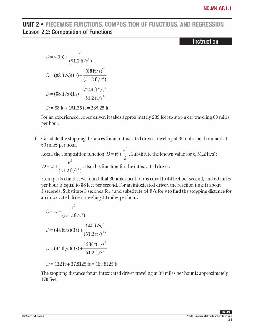
North Carolina Math 4 Teacher Resource 2.2
© Walch EducationU2-49
UNIT 2 • PIECEWISE FUNCTIONS, COMPOSITION OF FUNCTIONS, AND REGRESSIONLesson 2.2: Composition of Functions
Instruction
D vv
= +(1 s)(51.2 ft/s )
2
2
D= +(88 ft/s)(1 s)(88 ft/s)
(51.2 ft/s )
2
2
D= +(88 ft/s)(1 s)7744 ft /s
51.2 ft/s
2 2
2
D = 88 ft + 151.25 ft = 239.25 ft
For an experienced, sober driver, it takes approximately 239 feet to stop a car traveling 60 miles per hour.
f. Calculate the stopping distances for an intoxicated driver traveling at 30 miles per hour and at 60 miles per hour.
Recall the composition function D vtv
k= +
2
. Substitute the known value for k, 51.2 ft/s2:
D vtv
= +(51.2 ft/s )
2
2 . Use this function for the intoxicated driver.
From parts d and e, we found that 30 miles per hour is equal to 44 feet per second, and 60 miles per hour is equal to 88 feet per second. For an intoxicated driver, the reaction time is about 3 seconds. Substitute 3 seconds for t and substitute 44 ft/s for v to find the stopping distance for an intoxicated driver traveling 30 miles per hour:
D vtv
= +(51.2 ft/s )
2
2
D= +(44 ft/s)(3 s)(44 ft/s)
(51.2 ft/s )
2
2
D= +(44 ft/s)(3 s)1936 ft /s
51.2 ft/s
2 2
2
D = 132 ft + 37.8125 ft = 169.8125 ft
The stopping distance for an intoxicated driver traveling at 30 miles per hour is approximately 170 feet.
NC.M4.AF.1.1

North Carolina Math 4 Teacher Resource 2.2
© Walch EducationU2-50
UNIT 2 • PIECEWISE FUNCTIONS, COMPOSITION OF FUNCTIONS, AND REGRESSIONLesson 2.2: Composition of Functions
InstructionSubstitute 3 seconds for t and substitute 88 ft/s for v to find the stopping distance for an intoxicated driver traveling 60 miles per hour:
D vtv
= +(51.2 ft/s )
2
2
D= +(88 ft/s)(3 s)(88 ft/s)
(51.2 ft/s )
2
2
D= +(88 ft/s)(3 s)7744 ft/s
51.2 ft/s
2
2
D = 264 ft + 151.25 ft = 415.25 ft
The stopping distance for an intoxicated driver traveling at 60 miles per hour is approximately 415 feet.
g. How do the stopping distances differ for the sober driver and the intoxicated driver?
The approximate stopping distances are summarized in the following table.
Stopping Distances by Driver
30 mph 60 mphSober driver 82 ft 239 ftIntoxicated driver 170 ft 415 ft
At both speeds, the stopping distance that intoxicated drivers require is more than twice the stopping distance that sober drivers require.
h. Does doubling the speed of the car mean that it will take twice as far for the car to stop? Explain.
Recall that in the function D vtv
k= +
2
, vt represents the distance covered during the driver’s
reaction time and v
k
2
represents the distance covered from the moment the driver applies the
brake to the moment the car stops.
Looking only at the distance covered from the moment the driver applies the brake to the
moment the car stops, doubling the speed of the car leads to quadrupling the stopping distance.
For example, for a sober driver at 30 mph, this distance is 37.8125 ft, and for a sober driver
NC.M4.AF.1.1
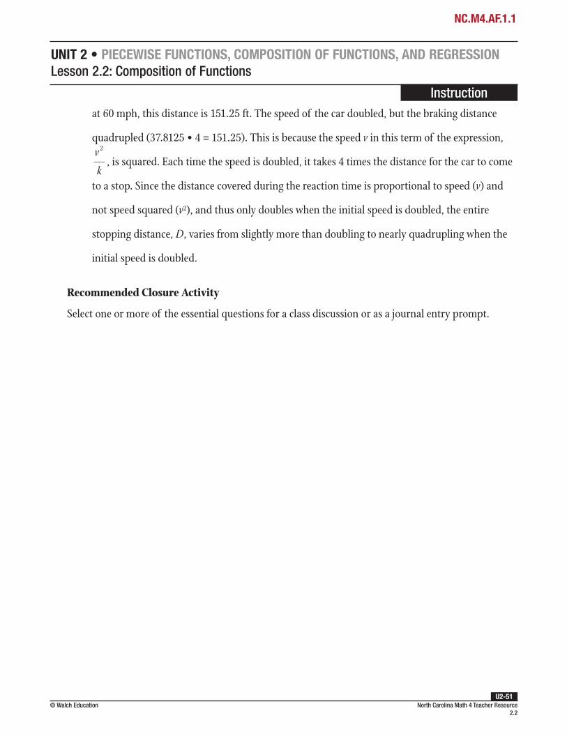
North Carolina Math 4 Teacher Resource 2.2
© Walch EducationU2-51
UNIT 2 • PIECEWISE FUNCTIONS, COMPOSITION OF FUNCTIONS, AND REGRESSIONLesson 2.2: Composition of Functions
Instructionat 60 mph, this distance is 151.25 ft. The speed of the car doubled, but the braking distance
quadrupled (37.8125 • 4 = 151.25). This is because the speed v in this term of the expression, v
k
2
, is squared. Each time the speed is doubled, it takes 4 times the distance for the car to come
to a stop. Since the distance covered during the reaction time is proportional to speed (v) and
not speed squared (v2), and thus only doubles when the initial speed is doubled, the entire
stopping distance, D, varies from slightly more than doubling to nearly quadrupling when the
initial speed is doubled.
Recommended Closure Activity
Select one or more of the essential questions for a class discussion or as a journal entry prompt.
NC.M4.AF.1.1

Practice 2.2: Composition of Functions A
Use ( ) 1f x x= − and g(x) = 5x to complete problems 1–8.
1. Find f(g(x)).
2. Find g(f(x)).
3. Find g(g(x)).
4. What is the domain of f(x)? Explain your answer.
5. What is the range of f(x)? Explain your answer.
6. Explain how to find the domain of f(g(x)), and find this domain.
7. Explain how to find the domain of g(f(x)), and find this domain.
8. What are the domain and range of g(g(x))? Explain your answer.
continued
North Carolina Math 4 Teacher Resource 2.2
© Walch EducationU2-52
Name: Date:UNIT 2 • PIECEWISE FUNCTIONS, COMPOSITION OF FUNCTIONS, AND REGRESSIONLesson 2.2: Composition of Functions
NC.M4.AF.1.1

Use the following scenario to complete problems 9 and 10.
Hannah is purchasing a new couch for her living room. At her favorite furniture store, the couch that she wants is on sale for 10% off the regular price of $1,000. She also has a $50 coupon for any item in the store. The store allows Hannah to use both the coupon and the 10% store discount, and she gets to decide the order in which she applies them to the price: the coupon first, then the 10% discount, or vice versa. The function C(p) = p – 50 represents the price when Hannah uses the coupon, and S(p) = 0.9p represents the price with the 10% discount, where p represents the regular price of the couch.
9. Find C(S(p)) and S(C(p)).
10. Based on the results of problem 9, which is the better deal—using the coupon first and then applying the 10% discount, or applying the 10% discount first and then using the coupon? Explain.
North Carolina Math 4 Teacher Resource 2.2
© Walch EducationU2-53
Name: Date:UNIT 2 • PIECEWISE FUNCTIONS, COMPOSITION OF FUNCTIONS, AND REGRESSIONLesson 2.2: Composition of Functions
NC.M4.AF.1.1

Use f(x) = 2x2 – 3x and g(x) = x + 4 to complete problems 1–6.
1. Find f(g(x)).
2. Find g(f(x)).
3. Find f(f(x)).
4. Find g(g(x)).
5. What are the domain and range of f(f(x))?
6. What are the domain and range of g(g(x))?
continued
Practice 2.2: Composition of Functions B
North Carolina Math 4 Teacher Resource 2.2
© Walch EducationU2-54
Name: Date:UNIT 2 • PIECEWISE FUNCTIONS, COMPOSITION OF FUNCTIONS, AND REGRESSIONLesson 2.2: Composition of Functions
NC.M4.AF.1.1
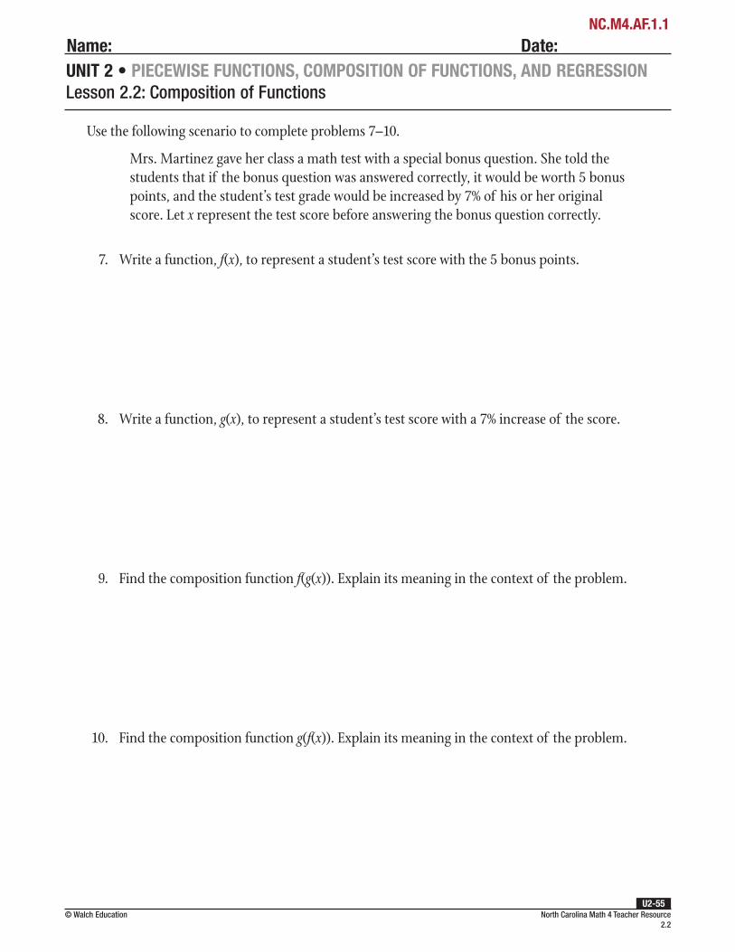
Use the following scenario to complete problems 7–10.
Mrs. Martinez gave her class a math test with a special bonus question. She told the students that if the bonus question was answered correctly, it would be worth 5 bonus points, and the student’s test grade would be increased by 7% of his or her original score. Let x represent the test score before answering the bonus question correctly.
7. Write a function, f(x), to represent a student’s test score with the 5 bonus points.
8. Write a function, g(x), to represent a student’s test score with a 7% increase of the score.
9. Find the composition function f(g(x)). Explain its meaning in the context of the problem.
10. Find the composition function g(f(x)). Explain its meaning in the context of the problem.
North Carolina Math 4 Teacher Resource 2.2
© Walch EducationU2-55
Name: Date:UNIT 2 • PIECEWISE FUNCTIONS, COMPOSITION OF FUNCTIONS, AND REGRESSIONLesson 2.2: Composition of Functions
NC.M4.AF.1.1
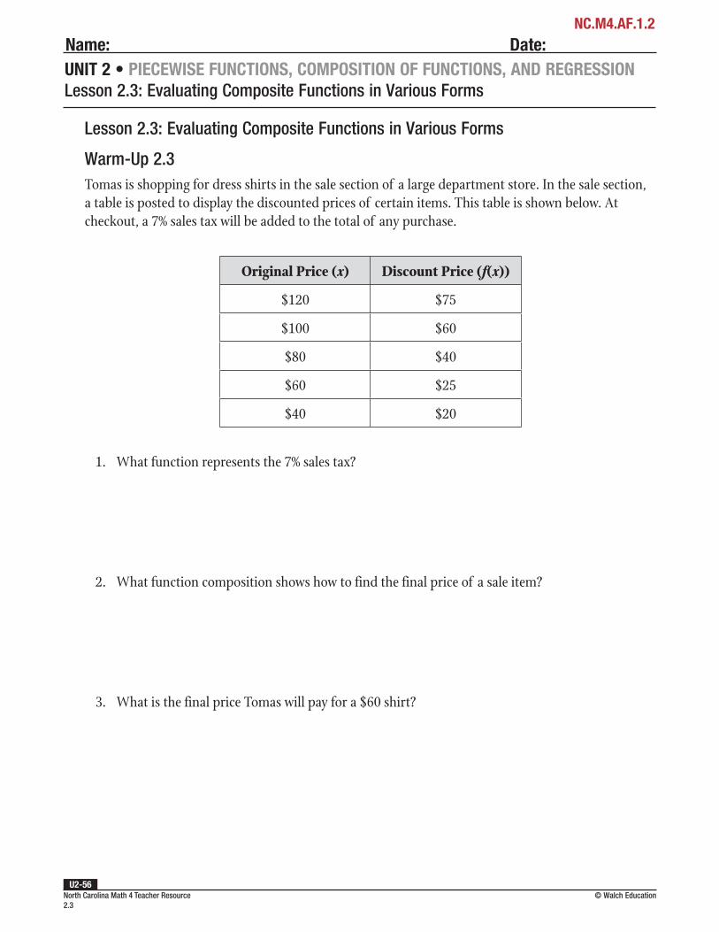
North Carolina Math 4 Teacher Resource 2.3
© Walch EducationU2-56
NC.M4.AF.1.2Name: Date:UNIT 2 • PIECEWISE FUNCTIONS, COMPOSITION OF FUNCTIONS, AND REGRESSIONLesson 2.3: Evaluating Composite Functions in Various Forms
Warm-Up 2.3Tomas is shopping for dress shirts in the sale section of a large department store. In the sale section, a table is posted to display the discounted prices of certain items. This table is shown below. At checkout, a 7% sales tax will be added to the total of any purchase.
Original Price (x) Discount Price (f(x))
$120 $75
$100 $60
$80 $40
$60 $25
$40 $20
1. What function represents the 7% sales tax?
2. What function composition shows how to find the final price of a sale item?
3. What is the final price Tomas will pay for a $60 shirt?
Lesson 2.3: Evaluating Composite Functions in Various Forms

North Carolina Math 4 Teacher Resource 2.3
© Walch EducationU2-57
Instruction
UNIT 2 • PIECEWISE FUNCTIONS, COMPOSITION OF FUNCTIONS, AND REGRESSIONLesson 2.3: Evaluating Composite Functions in Various Forms
Lesson 2.3: Evaluating Composite Functions in Various Forms
Warm-Up 2.3 Debrief1. What function represents the 7% sales tax?
If x represents the value of the original item, the sales tax adds 0.07x to the total. The amount paid would then be x + 0.07x. Therefore, the function is g(x) = 1.07x.
2. What function composition shows how to find the final price of a sale item?
To find the final price, first apply the function described in the table, f(x). Then, apply the sales tax function, g(x). The composition is g(f(x)).
3. What is the final price Tomas will pay for a $60 shirt?
To find the final price of a $60 shirt, find g(f(60)).
g(f(60)) = g(25) Evaluate f(60) using the table.
g(25) = 1.07 • 25 Substitute 25 into the formula for g(x).
g(25) = 26.75 Evaluate g(25).
Tomas will pay $26.75 for the shirt.
Connection to the Lesson
• Students determine from context which function in a composition to apply first.
• Students compose functions given in different forms.
NC.M4.AF.1.2
North Carolina Math 4 Standards
NC.M4.AF.1.2 Execute a procedure to determine the value of a composite function at a given value when the functions are in algebraic, graphical, or tabular representations.

North Carolina Math 4 Teacher Resource 2.3
© Walch EducationU2-58
Instruction
UNIT 2 • PIECEWISE FUNCTIONS, COMPOSITION OF FUNCTIONS, AND REGRESSIONLesson 2.3: Evaluating Composite Functions in Various Forms
IntroductionWhen using function composition as a modeling tool in mathematical situations, it is likely that the functions will appear in different forms. For example, perhaps one function is given in a table, while the other is given in a graph. It is important to develop familiarity evaluating function compositions in various forms.
Key Concepts• Recall that in a composition of functions, one function’s output becomes the other function’s input.
• When a function is given in a form other than an equation, the same process applies. For example, consider f(x) and g(x):
1 2 3 4 5
5
–1
–2
–3
–4
4
3
2
1
0
y
x
–5
–1–2–3–4–5
f(x)
x g(x)
–1 3
0 5
1 2
2 9
3 4
• The composition f(g(3)) can be found by evaluating g(3), then locating the result on the x-axis on the graph of x and finding the corresponding y-value.
Prerequisite Skills
This lesson requires the use of the following skills:
• composing functions (NC.M4.AF.1.1)
• evaluating functions given in various forms (F–IF.2)
NC.M4.AF.1.2

North Carolina Math 4 Teacher Resource 2.3
© Walch EducationU2-59
Instruction
UNIT 2 • PIECEWISE FUNCTIONS, COMPOSITION OF FUNCTIONS, AND REGRESSIONLesson 2.3: Evaluating Composite Functions in Various Forms
• In a real-world problem, the order in which to apply the functions may be found by analyzing the context.
• Recall that a composition can use the notation f(g(x)) or ( )( )f g x .
• If the function equations are given, the composite function can be graphed using a calculator.
On a TI-83/84:
Step 1: Enter your functions into the Y= menu.
Step 2: Enter the next equation and press [VARS].
Step 3: Press the right arrow key to enter the Y–VARS menu.
Step 4: Press [1] for Functions.
Step 5: Select the outer function of the composition from the menu.
Step 6: Press [(], then repeat steps 2–4 to return to the Functions list in the Y–VARS menu.
Step 7: Select the inner function of the composition from the menu.
Step 8: Press [)] and then [GRAPH] to graph the function.
On a TI-Nspire:
Step 1: Press the [doc] button. Arrow down to 4) Insert and select 4) Graph.
Step 2: Enter the first function of the composition as f1. The graph of f1 will appear.
Step 3: Repeat step 1, then enter the first function of the composition as f2. The graph of f2 will appear.
Step 4: Repeat step 1, then enter the composition using parentheses notation, e.g. f1(f2(x)). The graph of the composite function will appear.
Common Errors/Misconceptions
• confusing the order in which to evaluate a composition of functions
• confusing the inputs in a function composition
NC.M4.AF.1.2

North Carolina Math 4 Teacher Resource 2.3
© Walch EducationU2-60
NC.M4.AF.1.2Name: Date:UNIT 2 • PIECEWISE FUNCTIONS, COMPOSITION OF FUNCTIONS, AND REGRESSIONLesson 2.3: Evaluating Composite Functions in Various Forms
Use the functions to evaluate the compositions in problems 1–6.
f(x) = 3x – 1
x g(x)
0 –3
1 2
2 5
3 6
4 51 2 3 4 5
5
–1
–2
–3
–4
4
3
2
1
0
y
x
–5
–1–2–3–4–5
h(x)
1. ( )(3)f g
2. ( )(5)f h
3. ( )(1)g f
4. ( )( 3)−g h
5. ( )(0)h f
6. ( )(2)h g
continued
Scaffolded Practice 2.3: Evaluating Composite Functions in Various Forms

North Carolina Math 4 Teacher Resource 2.3
© Walch EducationU2-61
NC.M4.AF.1.2Name: Date:UNIT 2 • PIECEWISE FUNCTIONS, COMPOSITION OF FUNCTIONS, AND REGRESSIONLesson 2.3: Evaluating Composite Functions in Various Forms
Use the given information to complete problems 7–10.
Marina is checking out at a bookstore. She has a member card, which earns her a 15% discount on her purchase. She also has a $50 gift card.
7. Find a function f(x) to model the amount Marina must pay after a 15% discount on her purchase.
8. Find a function g(x) to model the amount Marina must pay after applying the gift card toward her purchase.
9. In what order must the functions be composed to find the amount Marina must pay after applying the discount but before the gift card?
10. Does the order of the functions in your composition matter?

North Carolina Math 4 Teacher Resource 2.3
© Walch EducationU2-62
Instruction
UNIT 2 • PIECEWISE FUNCTIONS, COMPOSITION OF FUNCTIONS, AND REGRESSIONLesson 2.3: Evaluating Composite Functions in Various Forms
Example 1
Find f(g(3)).
2 4 6 8 10
10
1 3 5 7 9
–2
–4
–6
–8
–9
–3
–5
–7
–1
8
6
4
2
7
5
3
1
0
9
y
x
–10
–1–2–3–4–5–6–7–8–9–10
f(x)
x g(x)
–2 5
–1 2
0 –5
1 –2
2 0
3 1
1. Determine the order to apply the functions.
The composition has g inside and f outside. Evaluate g first.
2. Evaluate the first function.
Use the table to evaluate g(3):
g(3) = 1
3. Evaluate the second function.
Using the output of the previous function, evaluate f:
f(1) = 1
Therefore, f(g(3)) = 1.
Guided Practice 2.3
NC.M4.AF.1.2

North Carolina Math 4 Teacher Resource 2.3
© Walch EducationU2-63
Instruction
UNIT 2 • PIECEWISE FUNCTIONS, COMPOSITION OF FUNCTIONS, AND REGRESSIONLesson 2.3: Evaluating Composite Functions in Various Forms
Example 2
Find f(g(8)).
f(x) = 1.45x
2 4 6 8 10
10
1 3 5 7 9
–2
–4
–6
–8
–9
–3
–5
–7
–1
8
6
4
2
7
5
3
1
0
9
y
x
–10
–1–2–3–4–5–6–7–8–9–10
g(x)
1. Determine the order to apply the functions.
The composition has g inside and f outside. Evaluate g first.
2. Evaluate the first function.
Use the graph to evaluate g(8):
g(8) = 6
3. Evaluate the second function.
Using the output of the previous function, evaluate f:
f(6) = 1.456 ≈ 9.2941
Therefore, f(g(8)) ≈ 9.2941.
NC.M4.AF.1.2

North Carolina Math 4 Teacher Resource 2.3
© Walch EducationU2-64
Instruction
UNIT 2 • PIECEWISE FUNCTIONS, COMPOSITION OF FUNCTIONS, AND REGRESSIONLesson 2.3: Evaluating Composite Functions in Various Forms
Example 3
Shelly has a mold sample growing in a Petri dish. Every 8 hours, she records the diameter of the colony, in millimeters, and uses this to estimate the cell population. She records the population estimates in a table.
Hours (t) 0 8 16 24 32 40
Estimated population (p(t)) 20 120 720 4,320 25,920 155,520
Later, she learns the population estimate function she was using was too large. Shelly determined that she could use the function g(x) = 0.85x to correct her estimates. What is the corrected population estimate for t = 40?
1. Determine the order to apply the functions.
The function g(x) takes the population estimate as inputs and outputs a different population estimate. The function p(t) takes time as inputs and outputs population. The function p(t) should be applied first.
2. Evaluate the first function.
At t = 40, p(t) = 155,520.
3. Evaluate the second function.
At x = 155,520, g(x) = 0.85 • 155,520 = 132,192.
The corrected population estimate is approximately 132,192 mold cells.
NC.M4.AF.1.2

North Carolina Math 4 Teacher Resource 2.3
© Walch EducationU2-65
Instruction
UNIT 2 • PIECEWISE FUNCTIONS, COMPOSITION OF FUNCTIONS, AND REGRESSIONLesson 2.3: Evaluating Composite Functions in Various Forms
Example 4
Let ( ) sin1
5cos 2( )= +
+
−f x e
xxx and ( ) 10 13 2= − + −g x x x x . Use a graphing calculator to
estimate (0.5)( )f g and (0.5)( )g f .
1. Graph the composition ( )( )f g x .
On a TI-83/84:
Step 1: Enter f(x) and g(x) into the Y= menu as Y1 and Y2.
Step 2: Enter Y3 in the Y= menu and press [VARS].
Step 3: Press the right arrow key to enter the Y–VARS menu.
Step 4: Press [1] for Functions.
Step 5: Select Y1 from the menu.
Step 6: Press [(], then repeat steps 2–4 to return to the Functions list in the Y–VARS menu.
Step 7: Select Y2 from the menu.
Step 8: Press [)] and then [GRAPH] to graph the function.
On a TI-Nspire:
Step 1: Press the [doc] button. Arrow down to 4: Insert and select 4: Graph.
Step 2: Define f1 = f(x).
Step 3: Repeat Step 1. Define f2 = g(x).
Step 4: Repeat Step 1. Define a third function f3 = f1(f2(x)). The graph of the composite function will appear.
(continued)
NC.M4.AF.1.2
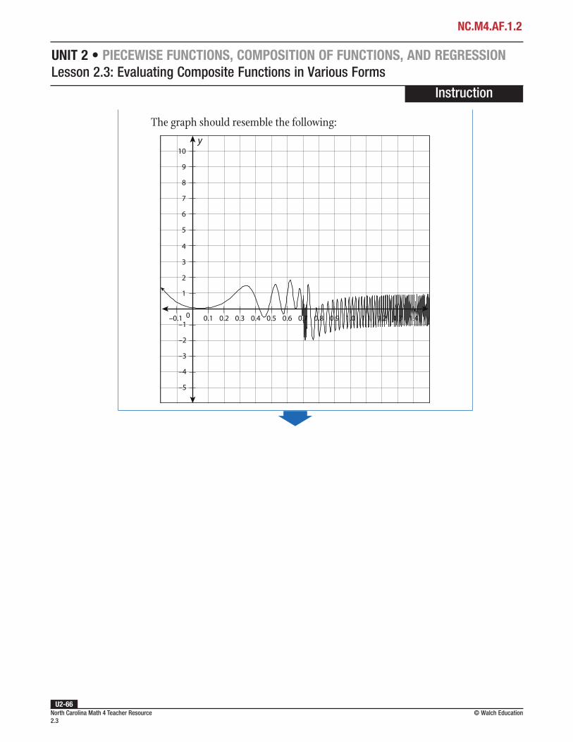
North Carolina Math 4 Teacher Resource 2.3
© Walch EducationU2-66
Instruction
UNIT 2 • PIECEWISE FUNCTIONS, COMPOSITION OF FUNCTIONS, AND REGRESSIONLesson 2.3: Evaluating Composite Functions in Various Forms
The graph should resemble the following:
0.2 0.4 0.6 0.8 1.00.1 0.3 0.5 0.7 0.9 1.2 1.41.1 1.3
10
–2
–4
–3
–5
–1
8
6
4
2
7
5
3
1
0
9
y
–0.1
NC.M4.AF.1.2

North Carolina Math 4 Teacher Resource 2.3
© Walch EducationU2-67
Instruction
UNIT 2 • PIECEWISE FUNCTIONS, COMPOSITION OF FUNCTIONS, AND REGRESSIONLesson 2.3: Evaluating Composite Functions in Various Forms
2. Use the graph to evaluate (0.5)( )f g .
Use the calculator’s Trace function to estimate (0.5)( )f g .
0.2 0.4 0.6 0.8 1.00.1 0.3 0.5 0.7 0.9 1.2 1.41.1 1.3
(0.5, 0.91)
10
–2
–4
–3
–5
–1
8
6
4
2
7
5
3
1
0
9
y
–0.1
From the graph, (0.5) 0.91( ) ≈f g .
NC.M4.AF.1.2

North Carolina Math 4 Teacher Resource 2.3
© Walch EducationU2-68
Instruction
UNIT 2 • PIECEWISE FUNCTIONS, COMPOSITION OF FUNCTIONS, AND REGRESSIONLesson 2.3: Evaluating Composite Functions in Various Forms
3. Graph the composition ( )( )g f x .
On a TI-83/84:
Step 1: Verify that f(x) and g(x) have been typed into the Y= menu as Y1 and Y2.
Step 2: Enter Y3 in the Y= menu and press [VARS].
Step 3: Press the right arrow key to enter the Y–VARS menu.
Step 4: Press [1] for Functions.
Step 5: Select Y2 from the menu.
Step 6: Press [(], then repeat steps 2–4 to return to the Functions list in the Y–VARS menu.
Step 7: Select Y1 from the menu.
Step 8: Press [)] and then [GRAPH] to graph the function.
On a TI-Nspire:
Step 1: Verify that f1 = f(x) and f2 = g(x).
Step 2: Press the [doc] button. Arrow down to 4: Insert and select 4: Graph.
Step 3: Define a new function f4 = f2(f1(x)). The graph of the function will appear.
(continued)
NC.M4.AF.1.2

North Carolina Math 4 Teacher Resource 2.3
© Walch EducationU2-69
Instruction
UNIT 2 • PIECEWISE FUNCTIONS, COMPOSITION OF FUNCTIONS, AND REGRESSIONLesson 2.3: Evaluating Composite Functions in Various Forms
The graph should resemble the following:
–40
–80
–120
–60
–100
–140
–20
120
80
40
140
100
60
20
y
x
1 20.5 1.5 2.50–0.5–1–1.5–2–2.5–3
NC.M4.AF.1.2

North Carolina Math 4 Teacher Resource 2.3
© Walch EducationU2-70
Instruction
UNIT 2 • PIECEWISE FUNCTIONS, COMPOSITION OF FUNCTIONS, AND REGRESSIONLesson 2.3: Evaluating Composite Functions in Various Forms
4. Use the graph to evaluate (0.5)( )g f .
Use the calculator’s Trace function to estimate (0.5)( )f g .
–40
–80
–120
–60
–100
–140
–20
120
80
40
140
100
60
20
y
x
1 20.5 1.5 2.50–0.5–1–1.5–2–2.5–3
(0.5, –6.91)
From the graph, (0.5) 6.91( ) ≈ −g f .
NC.M4.AF.1.2

North Carolina Math 4 Teacher Resource 2.3
© Walch EducationU2-71
NC.M4.AF.1.2Name: Date:UNIT 2 • PIECEWISE FUNCTIONS, COMPOSITION OF FUNCTIONS, AND REGRESSIONLesson 2.3: Evaluating Composite Functions in Various Forms
Karla is modeling the range of historical 6-inch cannons for a physics project. She has managed to find equations that model the motion of cannonballs while factoring in air resistance:
( ) ln2 2
0
2=+
P t
v
g
v gu t
vxT T
T
( )2
ln( )
20
2 2
2 2=++
P t
v
g
v v
V t vyT T
T
( )
tan
tan
0
0
=−
+
V t v
v vg
vt
v vg
vt
T
TT
TT
Karla made a table to keep track of all the variables in these equations, and filled in constant values with reasonable estimates she found through her research:
Variable DescriptionValue (with
units)
Px(t)distance travelled by the cannonball after t seconds
unknown (m)
Py(t) cannonball’s height at t seconds unknown (m)
V(t) cannonball’s vertical velocity at t seconds unknown (m/s)
u0 cannonball’s initial horizontal velocity 365 m/s
v0 cannonball’s initial vertical velocity 65 m/s
vT cannonball’s terminal velocity 150 m/s
g force due to gravity 9.8 m/s
t time unknown (s)
Help Karla use the equations and values to approximate the range of the cannon. What factors might affect this range?
Problem-Based Task 2.3: Cannon Fire
Help Karla use the equations and values to approximate the range of the cannon.
SMP 1 ✓ 2 ✓3 ✓ 4 ✓5 ✓ 6 ✓7 ✓ 8 ✓

North Carolina Math 4 Teacher Resource 2.3
© Walch EducationU2-72
NC.M4.AF.1.2Name: Date:UNIT 2 • PIECEWISE FUNCTIONS, COMPOSITION OF FUNCTIONS, AND REGRESSIONLesson 2.3: Evaluating Composite Functions in Various Forms
Problem-Based Task 2.3: Cannon Fire
Coaching Questionsa. What composition(s) and other strategies can help solve this problem?
b. What is a simpler form forV(t)?
c. What is a simpler form forPy(t)?
d. What is the significance of the intercepts of Py(t)?
e. What value(s) of t are important, and why are they important?
f. Is it easiest to find important values of t using a table, using a graph, or by solving equations?
g. How can you find the range of the historical cannons?
h. What factors might affect the range?

North Carolina Math 4 Teacher Resource 2.3
© Walch EducationU2-73
Instruction
UNIT 2 • PIECEWISE FUNCTIONS, COMPOSITION OF FUNCTIONS, AND REGRESSIONLesson 2.3: Evaluating Composite Functions in Various Forms
Problem-Based Task 2.3: Cannon Fire
Coaching Sample Responsesa. What composition(s) and other strategies can help solve this problem?
The equation Py(t) gives the height of the cannonball, and is given in terms of V(t). The composition ( ) ( )P V ty will be needed to find the time at which the cannonball hits the ground.
The equation Px(t) gives the horizontal distance travelled by a cannonball, but we’ll need the value of t when the cannonball hits the ground in order to solve for the maximum range.
b. What is a simpler form for V(t)?
Substitute values into V(t) and evaluate:
( )
tan
tan
0
0
=−
+
V t v
v vg
vt
v vg
vt
T
TT
TT
( ) 150
65 150 tan9.8
150
150 65 tan9.8
150
=−
+
V tt
t
( )9, 750 22, 500 tan 0.0653
320 75 tan 0.0653
( )( )=
−+
V tt
t
NC.M4.AF.1.2
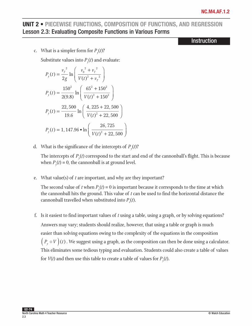
North Carolina Math 4 Teacher Resource 2.3
© Walch EducationU2-74
Instruction
UNIT 2 • PIECEWISE FUNCTIONS, COMPOSITION OF FUNCTIONS, AND REGRESSIONLesson 2.3: Evaluating Composite Functions in Various Forms
c. What is a simpler form forPy(t)?
Substitute values into Py(t) and evaluate:
( )2
ln( )
20
2 2
2 2=++
P t
v
g
v v
V t vyT T
T
( )150
2(9.8)ln
65 150
( ) 150
2 2 2
2 2=++
P t
V ty
( )22, 500
19.6ln
4, 225 22, 500
( ) 22, 5002=++
P tV ty
( ) 1, 147.96 • ln26, 725
( ) 22, 5002=+
P tV ty
d. What is the significance of the intercepts of Py(t)?
The intercepts of Py(t) correspond to the start and end of the cannonball’s flight. This is because when Py(t) = 0, the cannonball is at ground level.
e. What value(s) of t are important, and why are they important?
The second value of t when Py(t) = 0 is important because it corresponds to the time at which the cannonball hits the ground. This value of t can be used to find the horizontal distance the cannonball travelled when substituted into Px(t).
f. Is it easiest to find important values of t using a table, using a graph, or by solving equations?
Answers may vary; students should realize, however, that using a table or graph is much
easier than solving equations owing to the complexity of the equations in the composition
( )( )P V ty . We suggest using a graph, as the composition can then be done using a calculator.
This eliminates some tedious typing and evaluation. Students could also create a table of values
for V(t) and then use this table to create a table of values for Py(t).
NC.M4.AF.1.2

North Carolina Math 4 Teacher Resource 2.3
© Walch EducationU2-75
Instruction
UNIT 2 • PIECEWISE FUNCTIONS, COMPOSITION OF FUNCTIONS, AND REGRESSIONLesson 2.3: Evaluating Composite Functions in Various Forms
On a TI-83/84:
Step 1: Enter V(t) and Py(t) as Y1 and Y2.
Step 2: Enter the Y3 equation and press [VARS].
Step 3: Press the right arrow key to enter the Y–VARS menu.
Step 4: Press [1] for Functions.
Step 5: Select Y2 from the menu.
Step 6: Press [(], then repeat steps 2–4 to return to the Functions list in the Y–VARS menu.
Step 7: Select the Y1 from the menu.
Step 8: Press [)] and then [GRAPH] to graph the function.
On a TI-Nspire:
Step 1: Press the [doc] button. Arrow down to 4: Insert and select 4: Graph.
Step 2: Define f1 = V(t).
Step 3: Repeat Step 1. Define f2 = Py(t).
Step 4: Repeat Step 1. Define a third function f3 = f2(f1(x)). The graph of the function will appear.
Use the Trace function to approximate the value of t when ( ) 0( ) =P V ty on the graph.
2 4 6 8 10
200
160
120
80
40
140
100
60
20
180
1 3 5 7 9 12 1411 13 15
280
240
260
220
–20
(12.52, 0)
0
From the graph, t ≈ 12.52.
NC.M4.AF.1.2

North Carolina Math 4 Teacher Resource 2.3
© Walch EducationU2-76
Instruction
UNIT 2 • PIECEWISE FUNCTIONS, COMPOSITION OF FUNCTIONS, AND REGRESSIONLesson 2.3: Evaluating Composite Functions in Various Forms
g. How can you find the range of the historical cannons?
Evaluate Px(t) at t = 12.52:
( ) ln2 2
0
2=+
P t
v
g
v gu t
vxT T
T
( )150
9.8ln
150 (9.8)(365)(12.52)
150
2 2
2≈+
P tx
( ) 2, 295.92 • ln22, 500 44, 784.04
22, 500≈
+
P tx
( ) 2, 295.92 • ln67, 284.04
22, 500≈
P tx
Px(t) ≈ 2,295.92 • ln(2.9940)
Px(t) ≈ 2,295.92 • 1.0954078
Px(t) ≈ 2,514.67
The 6-inch cannon can launch a cannonball to a distance of approximately 2,500 meters.
h. What factors might affect the range?
Answers may vary. Mathematical factors that might affect the range include the initial velocities. This is tied to the real-world factor of the speed at which the cannonball leaves the barrel of the cannon, which could be affected by the amount of propellant used to launch the cannonball. The initial velocities could also be affected by the angle at which the cannonball is launched; a lower angle would make v0 lower.
Recommended Closure Activity
Select one or more of the essential questions for a class discussion or as a journal entry prompt.
NC.M4.AF.1.2

North Carolina Math 4 Teacher Resource 2.3
© Walch EducationU2-77
NC.M4.AF.1.2Name: Date:UNIT 2 • PIECEWISE FUNCTIONS, COMPOSITION OF FUNCTIONS, AND REGRESSIONLesson 2.3: Evaluating Composite Functions in Various Forms
Use the given functions to evaluate the compositions in problems 1–6.
f(x) = x2 – 5
x g(x)
–1 5
0 4
1 3
2 1
3 0
4 1
5 4
2 4 6 8 10
10
1 3 5 7 9
–2
–4
–6
–8
–9
–3
–5
–7
–1
8
6
4
2
7
5
3
1
0
9
y
x
–10
–1–2–3–4–5–6–7–8–9–10
h(x)
1. ( )(1)f g
2. ( )(6)f h
3. ( )(2)g f
4. ( )(1)g h
5. ( )(0)h f
6. ( )(5)h g
Practice 2.3: Evaluating Composite Functions in Various Forms A
continued

North Carolina Math 4 Teacher Resource 2.3
© Walch EducationU2-78
NC.M4.AF.1.2Name: Date:UNIT 2 • PIECEWISE FUNCTIONS, COMPOSITION OF FUNCTIONS, AND REGRESSIONLesson 2.3: Evaluating Composite Functions in Various Forms
Use the given information to solve problems 7 and 8.
Yan’s part-time job offers a commission bonus to employees who earn the company $10,000 or more in sales in a week. Let f(x) = x – 10,000 represent the sales amount eligible for a bonus. The amount paid as a bonus is shown below.
x 0 500 1,000 1,500 2,000 2,500 3,000
g(x) 50 50 100 100 100 125 150
7. How much would Yan earn if he made $10,000 in sales?
8. How much would Yan earn if he made $13,000 in sales?
Use a calculator to solve problems 9 and 10.
9. If f(x) = x •3x and ( )1
92=+
g xx
, find f(g(1)).
10. If f(x) = ln (x + 12) – x2 and g x x4 13(( )) == −− , find g(f(0)).

North Carolina Math 4 Teacher Resource 2.3
© Walch EducationU2-79
NC.M4.AF.1.2Name: Date:UNIT 2 • PIECEWISE FUNCTIONS, COMPOSITION OF FUNCTIONS, AND REGRESSIONLesson 2.3: Evaluating Composite Functions in Various Forms
Use the given functions to evaluate the compositions in problems 1–6.
f(x) = 0.25x + 1
x g(x)
–1 0.5
0 1
1 2
2 4
3 8
4 16
5 32
2 4 6 8 10
10
1 3 5 7 9
–2
–4
–6
–8
–9
–3
–5
–7
–1
8
6
4
2
7
5
3
1
0
9
y
x
–10
–1–2–3–4–5–6–7–8–9–10
1. ( )(2)f g
2. ( )(3)f h
3. ( )(8)g f
4. ( )(0)g h
5. ( )( 16)−h f
6. ( )(1)h g
Practice 2.3: Evaluating Composite Functions in Various Forms B
continued

North Carolina Math 4 Teacher Resource 2.3
© Walch EducationU2-80
NC.M4.AF.1.2Name: Date:UNIT 2 • PIECEWISE FUNCTIONS, COMPOSITION OF FUNCTIONS, AND REGRESSIONLesson 2.3: Evaluating Composite Functions in Various Forms
Use the given information to solve problems 7 and 8.
An appliance store is offering a sale of 20% off major appliances. Certain models also have manufacturer’s coupons available. Andy is shopping for a new refrigerator and compiled a table with the discounts available for the different models he likes.
Price (x) $200 $300 $350 $500 $600 $700 $750
Discounted price (p(x)) $180 $260 $300 $400 $450 $650 $600
7. Find a function to represent the store’s discount.
8. Suppose the manufacturer’s coupon is applied first. How much would Andy pay for the $600 refrigerator?
Use a calculator to solve problems 9 and 10.
9. If 1
2( ) = − +f x x xx
and ( ) 2 1= +g x x , find f(g(2)).
10. If f(x) = x3 log (x) and ( ) tan( )π=g x x , find g(f(1)).

North Carolina Math 4 Teacher Resource 2.4
© Walch EducationU2-81
NC.M4.AF.5.1Name: Date:UNIT 2 • PIECEWISE FUNCTIONS, COMPOSITION OF FUNCTIONS, AND REGRESSIONLesson 2.4: Linear, Exponential, and Quadratic Regression
Warm-Up 2.4
Jacob is tracking his spending on groceries. The following table records the average amount he spent on groceries each month for the past five years.
YearAverage
spending ($)
1 55
2 80
3 70
4 75
5 107
1. Create a scatter plot of the data.
2. Describe the shape of the points.
3. Jacob determines the line y = 10x + 50 can be used to model his spending, and predicts that he will spend about $110 each month next year. Graph the line on the scatter plot. Is this a reasonable estimate?
Lesson 2.4: Linear, Exponential, and Quadratic Regression

North Carolina Math 4 Teacher Resource 2.4
© Walch EducationU2-82
Instruction
UNIT 2 • PIECEWISE FUNCTIONS, COMPOSITION OF FUNCTIONS, AND REGRESSIONLesson 2.4: Linear, Exponential, and Quadratic Regression
Lesson 2.4: Linear, Exponential, and Quadratic Regression
Warm-Up 2.4 Debrief
1. Create a scatter plot of the data.
Let x represent the year and y represent Jacob’s average monthly spending.
90
50
10
120
70
30
0
y
x
2 43 5 61Year
Am
ount
spe
nt ($
)
110
60
20
130
80
40
100
2. Describe the shape of the points.
The points don’t seem to form a distinct shape, but they do seem to increase approximately linearly over the five years.
NC.M4.AF.5.1
North Carolina Math 4 Standard
NC.M4.AF.5.1 Construct regression models of linear, quadratic, exponential, logarithmic, & sinusoidal functions of bivariate data using technology to model data and solve problems.

North Carolina Math 4 Teacher Resource 2.4
© Walch EducationU2-83
Instruction
UNIT 2 • PIECEWISE FUNCTIONS, COMPOSITION OF FUNCTIONS, AND REGRESSIONLesson 2.4: Linear, Exponential, and Quadratic Regression
3. Jacob determines the line y = 10x + 50 can be used to model his spending, and predicts that he will spend about $110 each month next year. Graph the line on the scatter plot. Is this a reasonable estimate?
90
50
10
120
70
30
0
y
x
2 43 5 61Year
Am
ount
spe
nt ($
)
110
60
20
130
80
40
100
According to the graph, $110 is a reasonable estimate. Without more data, it is difficult to say how accurate the estimate is.
Connection to the Lesson
• Students will recognize that a set of data points in a scatter plot can have a linear, quadratic, or exponential trend.
• Students will determine whether a function that models the data is a good fit.
NC.M4.AF.5.1

North Carolina Math 4 Teacher Resource 2.4
© Walch EducationU2-84
Instruction
UNIT 2 • PIECEWISE FUNCTIONS, COMPOSITION OF FUNCTIONS, AND REGRESSIONLesson 2.4: Linear, Exponential, and Quadratic Regression
Introduction
Data with two quantitative variables can be represented using a scatter plot. A scatter plot is a graph of data in two variables on a coordinate plane, where each data pair is represented by a point.
Relationships between the two quantitative variables can be observed on the graph. Graphing a function on the same coordinate plane as a scatter plot for a data set allows us to see if the function is a good estimation of the relationship between the two variables in the data set. The graph and the equation of the function can be used to estimate coordinate pairs that are not included in the data set.
Functions that approximate the data can be found using regression analysis. Regression analysis is a set of statistical processes that fit a particular function model to a data set. The function being fitted to the data is called the regression model, or simply the regression.
Key Concepts• Data with two quantitative variables can be shown graphically on a scatter plot.
• To create a scatter plot, plot each pair of data as a point on a coordinate plane.
• To find a regression model, first identify the type of function that models the data best.
• The type of function used to estimate the data will depend on the shape of the data in the scatter plot:
• A scatter plot that can be estimated with a linear function will look approximately like a line.
• A scatter plot that can be estimated with a quadratic function will look approximately like a parabola.
• A scatter plot that can be estimated with an exponential function will look approximately like an exponential curve.
• The context of the problem can also sometimes suggest a particular model. For example, data about population growth can often be modeled using an exponential function.
Prerequisite Skills
This lesson requires the use of the following skills:
• plotting points on the coordinate plane (5.G.1)
• graphing linear functions (F–IF.7)
• graphing quadratic functions (F–IF.7)
• graphing exponential functions (F–IF.7)
• analyzing the graphs of functions (F–IF.4)
NC.M4.AF.5.1

North Carolina Math 4 Teacher Resource 2.4
© Walch EducationU2-85
Instruction
UNIT 2 • PIECEWISE FUNCTIONS, COMPOSITION OF FUNCTIONS, AND REGRESSIONLesson 2.4: Linear, Exponential, and Quadratic Regression
• There are many ways to find a regression model, most of which are quite complicated to calculate by hand. Fortunately, technology can be used to calculate regression models instead.
• Follow these steps to fit a function to data using a graphing calculator.
On a TI-83/84:
Step 1: Press [STAT] to bring up the statistics menu. The first option, 1: Edit, will already be highlighted. Press [ENTER].
Step 2: Arrow up to L1 and press [CLEAR], then [ENTER], to clear the list. Repeat this process to clear L2 and L3, if needed.
Step 3: Enter the ordered pairs in the L1 and L2 lists. Make sure to enter the x-coordinates in L1 and the y-coordinates in L2.
Step 4: Press [STAT]. Arrow to the CALC menu. Select the appropriate function model. (For linear regression, press 4: LinReg(ax + b). For quadratic regression, press 5: QuadReg. For exponential regression, press 0: ExpReg.)
Step 5: Press [(], then [2ND][1] to type “L1” for Xlist. Press [,], then [2ND][2] to type “L2” for Ylist. Press [)] to close the parentheses.
Step 6: Press [ENTER] to calculate. The parameter values will appear on the screen.
On a TI-Nspire:
Step 1: Press [home]. Arrow over to the spreadsheet icon, the fourth icon from the left, and press [enter].
Step 2: To clear the lists in your calculator, arrow up to the topmost cell of the table to highlight the entire column, then press [menu]. Choose 3: Data, then 4: Clear Data. Repeat for each column as necessary.
Step 3: Arrow up to the topmost cell of the first column, labeled “A.” Press [X][enter] to type x. Then, arrow over to the second column, labeled “B.” Press [Y][enter] to type y.
Step 4: Arrow down to cell A1 and enter the first x-value from the ordered pairs. Press [enter]. Enter the second x-value in cell A2 and so on.
Step 5: Move over to cell B1 and enter the first y-value. Press [enter]. Enter the second y-value in cell B2 and so on.
Step 6: To fit an equation to the data points, press [menu] and select 4: Statistics, then 1: Stat Calculations, then select the appropriate model type. (Press 3 for linear regressions. Press 6 for quadratic regressions. Press A for exponential regressions.). Select “x” from the X List pop-up menu. Press [tab] to move to the Y List pop-up menu, then select “y” from the options. Tab to “OK” and press [enter]. The parameter values will appear on the screen.
NC.M4.AF.5.1

North Carolina Math 4 Teacher Resource 2.4
© Walch EducationU2-86
Instruction
UNIT 2 • PIECEWISE FUNCTIONS, COMPOSITION OF FUNCTIONS, AND REGRESSIONLesson 2.4: Linear, Exponential, and Quadratic Regression
• To compare a data set and a function, plot the function on the same coordinate plane as the scatter plot of the data set.
• Graph a linear function by plotting at least two points and drawing a line through those points. Note that technology-generated linear regressions have the form y = mx + b.
• Graph a quadratic or exponential function by plotting at least five points. Connect the points with a curve. Note that technology-generated exponential regressions have the form y = abx or y = aebx, where e is Euler’s number.
• The number e is an irrational number approximately equal to 2.71828. It is used often in exponential models because it has nice mathematical properties.
• Technology-generated quadratic regressions have the form y = ax2 + bx + c.
• A function is a good fit for the data set if it passes closely to the data points and if some of the data points are above the curve and some are below the curve.
• Evaluating a function that has a similar shape as a data set can provide an estimate for data not included in the plotted data set.
• Evaluate a function algebraically for a given value of x or y by substituting the given value for x or y and solving for the remaining variable.
• Evaluate a function graphically for a given value of x or y by finding the point on the graph of the function with the known coordinate, then finding the corresponding x- or y-value of that point.
Common Errors/Misconceptions
• using a function model that is not a good fit to estimate a relationship between two variables (e.g. using a linear model to estimate an exponential relationship)
• confusing x and y when graphing data points or analyzing a graph
• confusing parameters in technology-generated regressions (e.g. confusing a and b in the exponential model y = abx)
NC.M4.AF.5.1

North Carolina Math 4 Teacher Resource 2.4
© Walch EducationU2-87
NC.M4.AF.5.1Name: Date:UNIT 2 • PIECEWISE FUNCTIONS, COMPOSITION OF FUNCTIONS, AND REGRESSIONLesson 2.4: Linear, Exponential, and Quadratic Regression
In problems 1–3, identify whether the data in the scatter plot suggests a linear, quadratic, or exponential relationship.
1.
2 4 6 8 100 1 3 5 7 9 12 1411 13 15
10
8
6
4
2
7
5
3
1
9
14
12
15
13
11
x–1
–1
y
2.
2 4 6 8 100 1 3 5 7 9 12 1411 13 15
10
8
6
4
2
7
5
3
1
9
14
12
15
13
11
x–1
–1
y
continued
Scaffolded Practice 2.4: Linear, Exponential, and Quadratic Regression

North Carolina Math 4 Teacher Resource 2.4
© Walch EducationU2-88
NC.M4.AF.5.1Name: Date:UNIT 2 • PIECEWISE FUNCTIONS, COMPOSITION OF FUNCTIONS, AND REGRESSIONLesson 2.4: Linear, Exponential, and Quadratic Regression
3.
2 4 6 8 100 1 3 5 7 9 12 1411 13 15
10
8
6
4
2
7
5
3
1
9
14
12
15
13
11
x–1
–1
y
In problems 4–6, use a calculator or other technology to find an equation of the specified type to model each data set.
4. linear
x 1 2 3 4 5 6
y 15 13 12 10 9 9
5. exponential
x 1 2 4 5 6
y 1 1 3 8 12
6. quadratic
x 1 2 4 5 6
y 9 5 1 1 3
continued
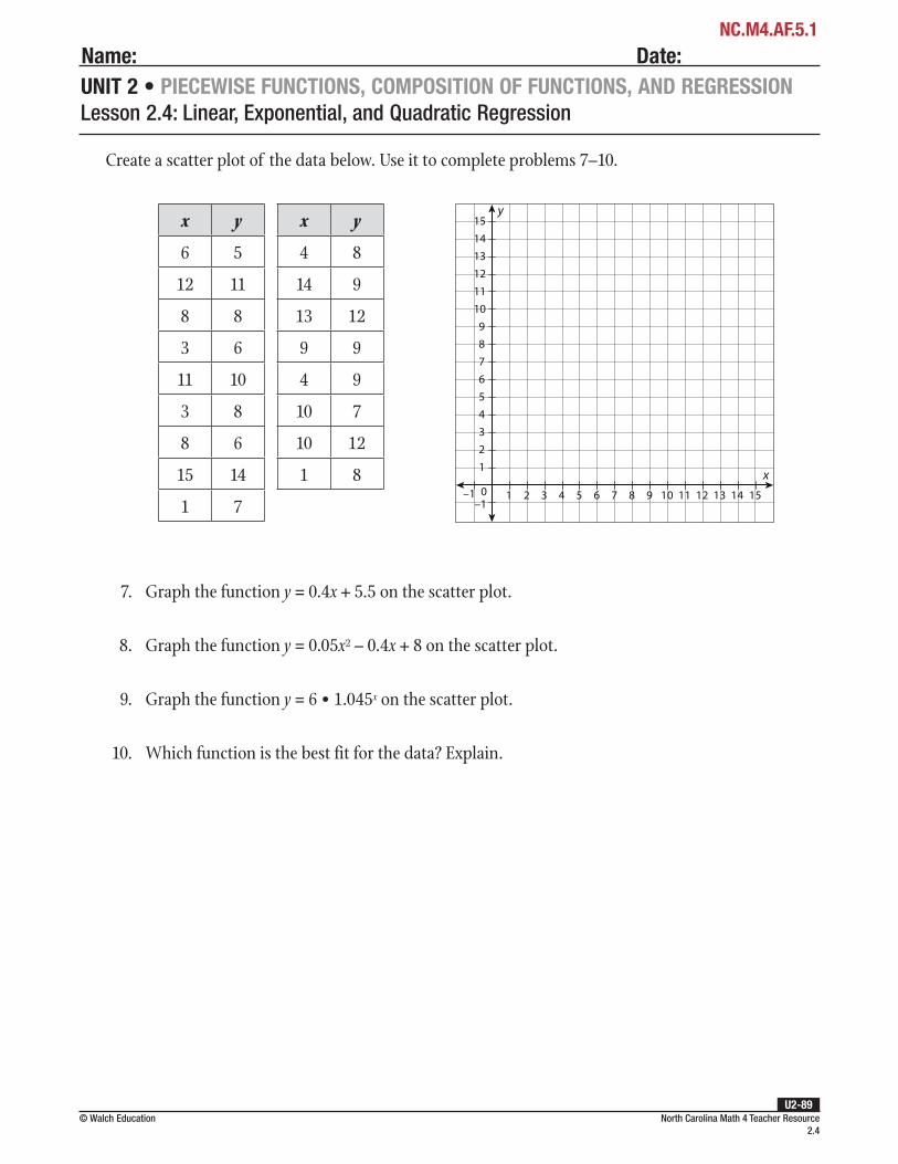
North Carolina Math 4 Teacher Resource 2.4
© Walch EducationU2-89
NC.M4.AF.5.1Name: Date:UNIT 2 • PIECEWISE FUNCTIONS, COMPOSITION OF FUNCTIONS, AND REGRESSIONLesson 2.4: Linear, Exponential, and Quadratic Regression
Create a scatter plot of the data below. Use it to complete problems 7–10.
x y x y
6 5 4 8
12 11 14 9
8 8 13 12
3 6 9 9
11 10 4 9
3 8 10 7
8 6 10 12
15 14 1 8
1 72 4 6 8 100 1 3 5 7 9 12 1411 13 15
10
8
6
4
2
7
5
3
1
9
14
12
15
13
11
x–1
–1
y
7. Graph the function y = 0.4x + 5.5 on the scatter plot.
8. Graph the function y = 0.05x2 – 0.4x + 8 on the scatter plot.
9. Graph the function y = 6 • 1.045x on the scatter plot.
10. Which function is the best fit for the data? Explain.

North Carolina Math 4 Teacher Resource 2.4
© Walch EducationU2-90
Instruction
UNIT 2 • PIECEWISE FUNCTIONS, COMPOSITION OF FUNCTIONS, AND REGRESSIONLesson 2.4: Linear, Exponential, and Quadratic Regression
Example 1
Thomas wants to know how long it will take his truck to stop based on how fast it is moving. The following table shows the distance the truck traveled after the brakes were applied while traveling at different speeds.
Speed (mph)Stopping
distance (ft)
10 420 2030 5040 6050 10560 160
Create a scatter plot showing the relationship between the speed of the truck and the distance it takes to stop once the brakes are applied. Show that the function y = 0.045x2 is a good estimate for the relationship between the speed and the stopping distance. About how far would it take the truck to stop if it were traveling at 70 mph?
1. Plot each point on the coordinate plane.
Let the x-axis represent the speed of the truck, and let the y-axis represent the stopping distance.
0
y
x
Stop
ping
dis
tanc
e (fe
et)
Speed (mph)20 40 60 80 10030 50 70 90 120 140110 130 15010
100
80
60
40
20
70
50
30
10
90
160
140
120
170
150
130
110
Guided Practice 2.4
NC.M4.AF.5.1

North Carolina Math 4 Teacher Resource 2.4
© Walch EducationU2-91
Instruction
UNIT 2 • PIECEWISE FUNCTIONS, COMPOSITION OF FUNCTIONS, AND REGRESSIONLesson 2.4: Linear, Exponential, and Quadratic Regression
2. Graph the given function on the coordinate plane.
The function is y = 0.045x2. Calculate the value of y for at least five different values of x. Start with x = 0, then calculate the value of the function for at least four more x-values in the data table.
x y
0 0.045(0)2 = 0
20 0.045(20)2 = 18
30 0.045(30)2 = 40.5
40 0.045(40)2 = 72
60 0.045(60)2 = 162
Plot these points on the same coordinate plane, then connect the points with a curve. Note: The new points are plotted as hollow dots.
0
Stop
ping
dis
tanc
e (fe
et)
Speed (mph)20 40 60 80 10030 50 70 90 120 140110 130 15010
100
80
60
40
20
70
50
30
10
90
160
140
120
170
150
130
110
y
x
NC.M4.AF.5.1

North Carolina Math 4 Teacher Resource 2.4
© Walch EducationU2-92
Instruction
UNIT 2 • PIECEWISE FUNCTIONS, COMPOSITION OF FUNCTIONS, AND REGRESSIONLesson 2.4: Linear, Exponential, and Quadratic Regression
Example 2
To learn more about the performance of an engine, engineers conduct tests and record the time it takes the car to reach certain speeds. A stopped car accelerates to 75 miles per hour. The following table shows the time, in seconds, after the car starts to accelerate and the speed it reaches at each time.
Time in seconds 0 1 2 3 4 5 6 7 8Speed in miles per hour
0 2.3 6.6 13.5 22.4 32.2 44.2 57.8 74.6
Does a linear, quadratic, or exponential function best model this data? Find the equation of the regression model that best fits the data.
3. Compare the graph of the function to the scatter plot of the data.
The graph of the function appears to be very close to the points in the scatter plot. Therefore, y = 0.045x2 is a good estimate of the data.
4. Use the equation to answer the question.
Use the equation to estimate the stopping distance when the truck is travelling 70 mph.
Evaluate the equation y = 0.045x2 for the speed of 70 mph, when x = 70.
y = 0.045(70)2 = 220.5
The equation y = 0.045x2 is a good estimate of the stopping distance of the truck. The stopping distance is approximately 220.5 feet when the truck is traveling 70 mph.
NC.M4.AF.5.1

North Carolina Math 4 Teacher Resource 2.4
© Walch EducationU2-93
Instruction
UNIT 2 • PIECEWISE FUNCTIONS, COMPOSITION OF FUNCTIONS, AND REGRESSIONLesson 2.4: Linear, Exponential, and Quadratic Regression
1. Create a scatter plot of the data set.
Let the x-axis represent the time, in seconds, and the y-axis represent the speed in miles.
55
35
15
70
45
25
0
y
x
2 43 5 61
Time (seconds)
Spee
d (m
iles
per h
our)
65
40
20
75
50
30
60
510
87 9 10
2. Determine if the data can be represented by a linear, quadratic, or exponential function.
The data appears to be curved, so either an exponential or a quadratic model should be used.
Recall that quadratic functions are used to model moving objects—specifically, falling objects, which fall due to the force of gravity. Gravity is a type of acceleration, so a quadratic model might be appropriate for this situation, too.
NC.M4.AF.5.1

North Carolina Math 4 Teacher Resource 2.4
© Walch EducationU2-94
Instruction
UNIT 2 • PIECEWISE FUNCTIONS, COMPOSITION OF FUNCTIONS, AND REGRESSIONLesson 2.4: Linear, Exponential, and Quadratic Regression
3. Find the equation of the regression model that best fits the data.
Use a calculator or other technology to find the regression equation.
On a TI-83/84:
Step 1: Press [STAT] to bring up the statistics menu. The first option, 1: Edit, will already be highlighted. Press [ENTER].
Step 2: Arrow up to L1 and press [CLEAR], then [ENTER], to clear the list. Repeat this process to clear L2 and L3, if needed.
Step 3: Enter the ordered pairs in the L1 and L2 lists. Make sure to enter the x-coordinates in L1 and the y-coordinates in L2.
Step 4: Press [STAT]. Arrow to the CALC menu. Press 5: QuadReg.
Step 5: Press [(], then [2ND][1] to type “L1” for Xlist. Press [,], then [2ND][2] to type “L2” for Ylist. Press [)] to close the parentheses.
Step 6: Press [ENTER] to calculate. The parameter values will appear on the screen.
(continued)
NC.M4.AF.5.1

North Carolina Math 4 Teacher Resource 2.4
© Walch EducationU2-95
Instruction
UNIT 2 • PIECEWISE FUNCTIONS, COMPOSITION OF FUNCTIONS, AND REGRESSIONLesson 2.4: Linear, Exponential, and Quadratic Regression
On a TI-Nspire:
Step 1: Press [home]. Arrow over to the spreadsheet icon, the fourth icon from the left, and press [enter].
Step 2: To clear the lists in your calculator, arrow up to the topmost cell of the table to highlight the entire column, then press [menu]. Choose 3: Data, then 4: Clear Data. Repeat for each column as necessary.
Step 3: Arrow up to the topmost cell of the first column, labeled “A.” Press [X][enter] to type x. Then, arrow over to the second column, labeled “B.” Press [Y][enter] to type y.
Step 4: Arrow down to cell A1 and enter the first x-value from the ordered pairs. Press [enter]. Enter the second x-value in cell A2 and so on.
Step 5: Move over to cell B1 and enter the first y-value. Press [enter]. Enter the second y-value in cell B2 and so on.
Step 6: To fit an equation to the data points, press [menu] and select 4: Statistics, then 1: Stat Calculations, then press 6 for quadratic regressions. Select “x” from the X List pop-up menu. Press [tab] to move to the Y List pop-up menu, then select “y” from the options. Tab to “OK” and press [enter]. The parameter values will appear on the screen.
The equation of the quadratic function is y = 0.95x2 + 1.71x – 0.2.
NC.M4.AF.5.1

North Carolina Math 4 Teacher Resource 2.4
© Walch EducationU2-96
Instruction
UNIT 2 • PIECEWISE FUNCTIONS, COMPOSITION OF FUNCTIONS, AND REGRESSIONLesson 2.4: Linear, Exponential, and Quadratic Regression
4. Plot the equation on the scatter plot and evaluate the fit.
Evaluate the function for at least five values of x. Plot the x-y coordinates on the scatter plot. Then draw a curve to connect them.
x 0 1 2 3 4 5 6 7 8
y –0.2 2.5 7 13.5 21.8 32.1 44.3 58.3 74.3
55
35
15
70
45
25
0
y
x
2 43 5 61
Time (seconds)
Spee
d (m
iles
per h
our)
65
40
20
75
50
30
60
510
87 9 10
The function appears to be a good fit for the data.
NC.M4.AF.5.1

North Carolina Math 4 Teacher Resource 2.4
© Walch EducationU2-97
Instruction
UNIT 2 • PIECEWISE FUNCTIONS, COMPOSITION OF FUNCTIONS, AND REGRESSIONLesson 2.4: Linear, Exponential, and Quadratic Regression
Example 3
Kanna starts a new hashtag on her social media, and it immediately starts trending. She records the number of total usages over the next week in the following table.
Day Uses
1 16
2 65
3 206
4 1,024
5 4,032
6 16,301
7 65,229
Does a linear, quadratic, or exponential function best model this data? Find the equation of the regression model that best fits the data. Use the model to predict how many times the hashtag might be used after 10 days.
1. Create a scatter plot of the data set.
Let the x-axis represent the day and the y-axis represent the number of times the hashtag was used on that day.
30,000
60,000
10,000
0
y
x
2 43 5 61
Days
Use
s
50,000
70,000
20,000
40,000
7 8
NC.M4.AF.5.1

North Carolina Math 4 Teacher Resource 2.4
© Walch EducationU2-98
Instruction
UNIT 2 • PIECEWISE FUNCTIONS, COMPOSITION OF FUNCTIONS, AND REGRESSIONLesson 2.4: Linear, Exponential, and Quadratic Regression
2. Determine if the data can be represented by a linear, quadratic, or exponential function.
The data appears to be curved, so either an exponential or a quadratic model should be used.
The beginning of the curve is fairly flat, which we would not expect in a quadratic model. Use an exponential function.
3. Find the equation of the regression model that best fits the data.
Use a calculator or other technology to find the regression equation.
On a TI-83/84:
Step 1: Press [STAT] to bring up the statistics menu. The first option, 1: Edit, will already be highlighted. Press [ENTER].
Step 2: Arrow up to L1 and press [CLEAR], then [ENTER], to clear the list. Repeat this process to clear L2 and L3, if needed.
Step 3: Enter the ordered pairs in the L1 and L2 lists. Make sure to enter the x-coordinates in L1 and the y-coordinates in L2.
Step 4: Press [STAT]. Arrow to the CALC menu. Press 0: ExpReg.
Step 5: Press [(], then [2ND][1] to type “L1” for Xlist. Press [,], then [2ND][2] to type “L2” for Ylist. Press [)] to close the parentheses.
Step 6: Press [ENTER] to calculate. The parameter values will appear on the screen.
(continued)
NC.M4.AF.5.1

North Carolina Math 4 Teacher Resource 2.4
© Walch EducationU2-99
Instruction
UNIT 2 • PIECEWISE FUNCTIONS, COMPOSITION OF FUNCTIONS, AND REGRESSIONLesson 2.4: Linear, Exponential, and Quadratic Regression
On a TI-Nspire:
Step 1: Press [home]. Arrow over to the spreadsheet icon, the fourth icon from the left, and press [enter].
Step 2: To clear the lists in your calculator, arrow up to the topmost cell of the table to highlight the entire column, then press [menu]. Choose 3: Data, then 4: Clear Data. Repeat for each column as necessary.
Step 3: Arrow up to the topmost cell of the first column, labeled “A.” Press [X][enter] to type x. Then, arrow over to the second column, labeled “B.” Press [Y][enter] to type y.
Step 4: Arrow down to cell A1 and enter the first x-value from the ordered pairs. Press [enter]. Enter the second x-value in cell A2 and so on.
Step 5: Move over to cell B1 and enter the first y-value. Press [enter]. Enter the second y-value in cell B2 and so on.
Step 6: To fit an equation to the data points, press [menu] and select 4: Statistics, then 1: Stat Calculations, then press A for exponential regressions. Select “x” from the X List pop-up menu. Press [tab] to move to the Y List pop-up menu, then select “y” from the options. Tab to “OK” and press [enter]. The parameter values will appear on the screen.
The equation of the quadratic function is y = 3.79 • 4.01x.
NC.M4.AF.5.1

North Carolina Math 4 Teacher Resource 2.4
© Walch EducationU2-100
Instruction
UNIT 2 • PIECEWISE FUNCTIONS, COMPOSITION OF FUNCTIONS, AND REGRESSIONLesson 2.4: Linear, Exponential, and Quadratic Regression
4. Plot the equation on the scatter plot and evaluate the fit.
Evaluate the function for at least five values of x. Plot the x-y coordinates on the scatter plot. Then draw a curve to connect them.
x 1 2 3 4 5 6 7
y 15.25 61.31 246.53 991.28 3,985.89 16,027.1 64,444.25
30,000
60,000
10,000
0
y
x
2 43 5 61
Days
Use
s
50,000
70,000
20,000
40,000
7 8
The function appears to be a good fit for the data.
5. Use the model to predict how many times the hashtag might be used after 10 days.
Evaluate the equation y = 3.79 • 4.01x for day 10, when x = 10.
y = 3.79 • 4.01x ≈ 4,074,581
If the pattern continues, the hashtag could be used more than 4 million times after 10 days.
NC.M4.AF.5.1

North Carolina Math 4 Teacher Resource 2.4
© Walch EducationU2-101
NC.M4.AF.5.1Name: Date:UNIT 2 • PIECEWISE FUNCTIONS, COMPOSITION OF FUNCTIONS, AND REGRESSIONLesson 2.4: Linear, Exponential, and Quadratic Regression
Sasha has a soil sample from Chernobyl that contains strontium-90. Strontium-90 is a radioactive element that is found in nature only in areas where nuclear explosions or accidents have occurred. It gives off large amounts of beta radiation.
Sasha performs an experiment. Every six months, he opens the sample, sets up his Geiger counter, and records the measured radiation level. He records the results in the following table.
YearRadioactivity
(µSv/hr)
0 12.68
0.5 12.53
1 12.38
1.5 12.23
2 12.09
2.5 11.94
3 11.81
3.5 11.66
4 11.52
4.5 11.38
Sasha thinks that the function y = –0.29x + 12.67 is the best fit for the data. Create a scatter plot of the data and graph this function with it. Then find another regression model for the data and graph it on another scatter plot. Which function is better, and why?
SMP 1 ✓ 2 ✓3 ✓ 4 ✓5 ✓ 6 ✓7 ✓ 8 ✓
Problem-Based Task 2.4: Fallout Records
Which function is better, and why?

North Carolina Math 4 Teacher Resource 2.4
© Walch EducationU2-102
NC.M4.AF.5.1Name: Date:UNIT 2 • PIECEWISE FUNCTIONS, COMPOSITION OF FUNCTIONS, AND REGRESSIONLesson 2.4: Linear, Exponential, and Quadratic Regression
Problem-Based Task 2.4: Fallout Records
Coaching Questions
a. Create a scatter plot of the data.
b. Graph the function y = –0.29x + 12.67 on the scatter plot.
c. Is this function a good fit for the data?
d. Would a quadratic or an exponential function fit the data better?
e. Use your chosen function type to find a regression model for the data.
f. Create a second scatter plot. Graph your regression model on it.
g. Is this function a good fit for the data?
h. Which function is a better fit for the data? Why?

North Carolina Math 4 Teacher Resource 2.4
© Walch EducationU2-103
Instruction
UNIT 2 • PIECEWISE FUNCTIONS, COMPOSITION OF FUNCTIONS, AND REGRESSIONLesson 2.4: Linear, Exponential, and Quadratic Regression
Problem-Based Task 2.4: Fallout Records
Coaching Sample Responses
a. Create a scatter plot of the data.
12
11.2
12.6
11.6
0
y
x2 43 51
Years
Radi
oact
ivity
(µSv
)
12.4
11.4
12.8
11.8
11
12.2
b. Graph the function y = –0.29x + 12.67 on the scatter plot.
12
11.2
12.6
11.6
0
y
x2 43 51
Years
Radi
oact
ivity
(µSv
)
12.4
11.4
12.8
11.8
11
12.2
c. Is this function a good fit for the data?
The data lies fairly close to the line. This function appears to be a good fit for the data.
NC.M4.AF.5.1

North Carolina Math 4 Teacher Resource 2.4
© Walch EducationU2-104
Instruction
UNIT 2 • PIECEWISE FUNCTIONS, COMPOSITION OF FUNCTIONS, AND REGRESSIONLesson 2.4: Linear, Exponential, and Quadratic Regression
d. Would a quadratic or an exponential function fit the data better?
Answers may vary. Either model would have to be sufficiently flattened that it would be difficult to tell just by looking which would be better. However, radioactive decay problems are usually modeled by exponential functions. Use an exponential function to model the data.
e. Use your chosen function type to find a regression model for the data.
On a TI-83/84:
Step 1: Press [STAT] to bring up the statistics menu. The first option, 1: Edit, will already be highlighted. Press [ENTER].
Step 2: Arrow up to L1 and press [CLEAR], then [ENTER], to clear the list. Repeat this process to clear L2 and L3, if needed.
Step 3: Enter the ordered pairs in the L1 and L2 lists. Make sure to enter the x-coordinates in L1 and the y-coordinates in L2.
Step 4: Press [STAT]. Arrow to the CALC menu. Press 0: ExpReg.
Step 5: Press [(], then [2ND][1] to type “L1” for Xlist. Press [,], then [2ND][2] to type “L2” for Ylist. Press [)] to close the parentheses.
Step 6: Press [ENTER] to calculate. The parameter values will appear on the screen.
On a TI-Nspire:
Step 1: Press [home]. Arrow over to the spreadsheet icon, the fourth icon from the left, and press [enter].
Step 2: To clear the lists in your calculator, arrow up to the topmost cell of the table to highlight the entire column, then press [menu]. Choose 3: Data, then 4: Clear Data. Repeat for each column as necessary.
Step 3: Arrow up to the topmost cell of the first column, labeled “A.” Press [X][enter] to type x. Then, arrow over to the second column, labeled “B.” Press [Y][enter] to type y.
Step 4: Arrow down to cell A1 and enter the first x-value from the ordered pairs. Press [enter]. Enter the second x-value in cell A2 and so on.
Step 5: Move over to cell B1 and enter the first y-value. Press [enter]. Enter the second y-value in cell B2 and so on.
Step 6: To fit an equation to the data points, press [menu] and select 4: Statistics, then 1: Stat Calculations, then press A for exponential regressions. Select “x” from the X List pop-up menu. Press [tab] to move to the Y List pop-up menu, then select “y” from the options. Tab to “OK” and press [enter]. The parameter values will appear on the screen.
The equation is y = 12.68 • 0.98x.
NC.M4.AF.5.1

North Carolina Math 4 Teacher Resource 2.4
© Walch EducationU2-105
Instruction
UNIT 2 • PIECEWISE FUNCTIONS, COMPOSITION OF FUNCTIONS, AND REGRESSIONLesson 2.4: Linear, Exponential, and Quadratic Regression
f. Create a second scatter plot. Graph your regression model on it.
12
11.2
12.6
11.6
0
y
x2 43 51
Years
Radi
oact
ivity
(µSv
)12.4
11.4
12.8
11.8
11
12.2
g. Is this function a good fit for the data?
The data lies fairly close to the line. This function appears to be a good fit for the data.
h. Which function is a better fit for the data? Why?
Answers may vary. Both functions appear to fit the data well. However, radioactive decay is typically modeled by exponential functions. For this reason, the exponential function may be a better choice.
Recommended Closure Activity
Select one or more of the essential questions for a class discussion or as a journal entry prompt.
NC.M4.AF.5.1
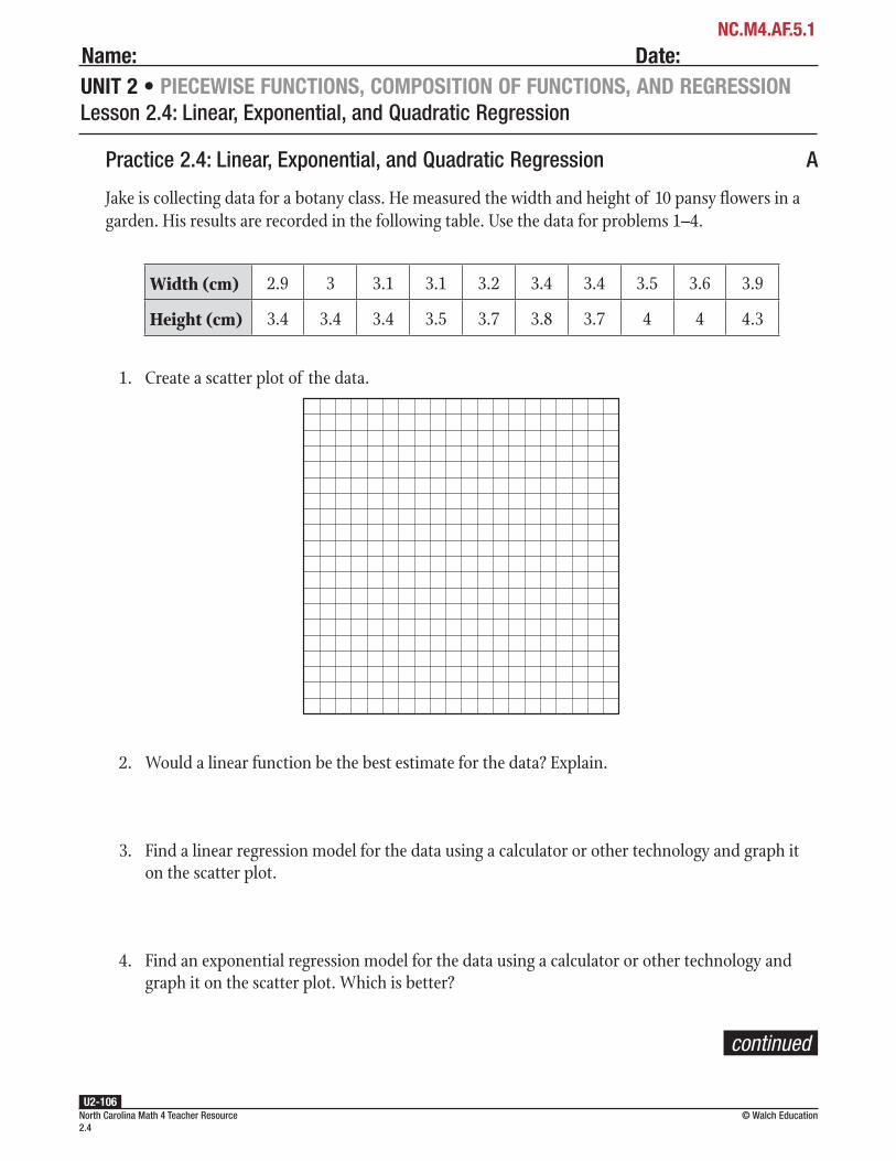
North Carolina Math 4 Teacher Resource 2.4
© Walch EducationU2-106
NC.M4.AF.5.1Name: Date:UNIT 2 • PIECEWISE FUNCTIONS, COMPOSITION OF FUNCTIONS, AND REGRESSIONLesson 2.4: Linear, Exponential, and Quadratic Regression
Jake is collecting data for a botany class. He measured the width and height of 10 pansy flowers in a garden. His results are recorded in the following table. Use the data for problems 1–4.
Width (cm) 2.9 3 3.1 3.1 3.2 3.4 3.4 3.5 3.6 3.9
Height (cm) 3.4 3.4 3.4 3.5 3.7 3.8 3.7 4 4 4.3
1. Create a scatter plot of the data.
2. Would a linear function be the best estimate for the data? Explain.
3. Find a linear regression model for the data using a calculator or other technology and graph it on the scatter plot.
4. Find an exponential regression model for the data using a calculator or other technology and graph it on the scatter plot. Which is better?
Practice 2.4: Linear, Exponential, and Quadratic Regression A
continued

North Carolina Math 4 Teacher Resource 2.4
© Walch EducationU2-107
NC.M4.AF.5.1Name: Date:UNIT 2 • PIECEWISE FUNCTIONS, COMPOSITION OF FUNCTIONS, AND REGRESSIONLesson 2.4: Linear, Exponential, and Quadratic Regression
The following table shows the population of Charlotte, North Carolina, from 1900 to 2010. Use the data for problems 5–7.
Year Entry Population
1900 1 18,091
1910 2 34,014
1920 3 46,338
1930 4 82,675
1940 5 100,899
1950 6 134,042
1960 7 201,564
1970 8 241,420
1980 9 315,474
1990 10 395,934
2000 11 540,828
2010 12 738,534
5. Create a scatter plot of the data.
continued

North Carolina Math 4 Teacher Resource 2.4
© Walch EducationU2-108
NC.M4.AF.5.1Name: Date:UNIT 2 • PIECEWISE FUNCTIONS, COMPOSITION OF FUNCTIONS, AND REGRESSIONLesson 2.4: Linear, Exponential, and Quadratic Regression
6. Would a linear, quadratic, or exponential function be the best estimate for the data? Explain.
7. Find a regression model for the data using a calculator or other technology and graph it on the scatter plot. Is it a good fit for the data?
The data in the following table and graph shows the horizontal distance (in feet) traveled by a golf ball hit at various angles. Use the data for problems 8–10.
Angle (°) Distance (ft)
5 507
9 560
13 582
17 587
21 580
25 565
600
400
200
700
500
300
100
0 4 82 6 10
x
12 1614 18 20 24 2822 26
y
Angle (°)
Dis
tanc
e (ft
)
8. Would a linear, quadratic, or exponential function be the best estimate for the data? Explain.
9. Find a regression model for the data using a calculator or other technology and graph it on the scatter plot. Is it a good fit for the data?
10. How far would you expect a golf ball hit at 16° to travel horizontally?

North Carolina Math 4 Teacher Resource 2.4
© Walch EducationU2-109
NC.M4.AF.5.1Name: Date:UNIT 2 • PIECEWISE FUNCTIONS, COMPOSITION OF FUNCTIONS, AND REGRESSIONLesson 2.4: Linear, Exponential, and Quadratic Regression
Anna is collecting data for a science project. She measured the circumference and weight of 10 Asian pears from trees around her area. Her results are recorded in the following table. Use the data for problems 1–4.
Diameter (inches) 2.1 2.1 2.5 3 3.3 3.3 3.3 3.4 3.4 3.4
Weight (ounces) 3.3 3.4 5.7 9.8 12.5 12.8 12.9 14 14.1 14.2
1. Create a scatter plot of the data.
2. Is a linear function a good fit for this data? Explain.
3. Find a linear regression model for the data using a calculator or other technology and graph it on the scatter plot.
4. Find a quadratic regression model for the data using a calculator or other technology and graph it on the scatter plot. Which is better?
Practice 2.4: Linear, Exponential, and Quadratic Regression B
continued

North Carolina Math 4 Teacher Resource 2.4
© Walch EducationU2-110
NC.M4.AF.5.1Name: Date:UNIT 2 • PIECEWISE FUNCTIONS, COMPOSITION OF FUNCTIONS, AND REGRESSIONLesson 2.4: Linear, Exponential, and Quadratic Regression
The following tabled show the estimated values for 12 pre-owned cars. Use the data for problems 5–7.
Age Price Age Price
0 $43,397 7 $19,068
1 $35,675 8 $16,774
2 $34,164 9 $14,775
3 $31,306 10 $12,792
4 $29,345 11 $10,283
5 $23,327 12 $9,519
6 $21,213
5. Create a scatter plot of the data.
6. Would a linear, quadratic, or exponential function be the best estimate for the data? Explain.
7. Find a regression model for the data using a calculator or other technology and graph it on the scatter plot. Is it a good fit for the data?
continued
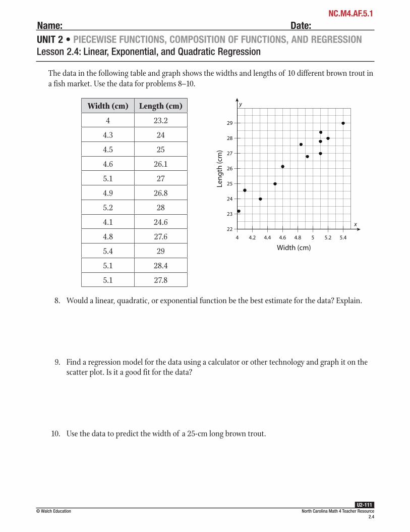
North Carolina Math 4 Teacher Resource 2.4
© Walch EducationU2-111
NC.M4.AF.5.1Name: Date:UNIT 2 • PIECEWISE FUNCTIONS, COMPOSITION OF FUNCTIONS, AND REGRESSIONLesson 2.4: Linear, Exponential, and Quadratic Regression
The data in the following table and graph shows the widths and lengths of 10 different brown trout in a fish market. Use the data for problems 8–10.
Width (cm) Length (cm)
4 23.2
4.3 24
4.5 25
4.6 26.1
5.1 27
4.9 26.8
5.2 28
4.1 24.6
4.8 27.6
5.4 29
5.1 28.4
5.1 27.8
4.4 4.84.2 4.6 5
28
26
24
29
27
25
23
y
x
5.2 5.44
Width (cm)
Leng
th (c
m)
22
8. Would a linear, quadratic, or exponential function be the best estimate for the data? Explain.
9. Find a regression model for the data using a calculator or other technology and graph it on the scatter plot. Is it a good fit for the data?
10. Use the data to predict the width of a 25-cm long brown trout.

North Carolina Math 4 Teacher Resource 2.5
© Walch EducationU2-112
UNIT 2 • PIECEWISE FUNCTIONS, COMPOSITION OF FUNCTIONS, AND REGRESSIONLesson 2.5: Analyzing Residual Plots
Name: Date:NC.M4.AF.5.2
Warm-Up 2.5Felicia is learning to ride a unicycle. She started at her house, which is considered to be at the origin of a coordinate plane. She went 2 blocks east and wasn’t able to successfully ride the unicycle. Then she started going north toward her friend’s house. After many failed attempts and falling off for 4 blocks, she had success for 2 blocks.
1. Plot the points (2, 4) and (2, 6) on a coordinate plane.
2. Find the distance between the two points. How far did Felicia successfully ride her unicycle?
3. Felicia is going to sell unicycle pins to raise money for medical research. She spent $2 of her own money to buy the pins and will sell each pin for $4. Her revenue can be modeled by the function y = 4x – 2. Plot the function y = 4x – 2 over the domain of all real numbers.
Lesson 2.5: Analyzing Residual Plots

North Carolina Math 4 Teacher Resource 2.5
© Walch EducationU2-113
UNIT 2 • PIECEWISE FUNCTIONS, COMPOSITION OF FUNCTIONS, AND REGRESSIONLesson 2.5: Analyzing Residual Plots
Instruction
NC.M4.AF.5.2
Warm-Up 2.5 Debrief1. Plot the points (2, 4) and (2, 6) on a coordinate plane.
The first number in each ordered pair is the x-value, and the second number is the y-value.
2 4 6 8 10
10
9
8
7
6
5
4
3
2
1
1 3 5 7 90
x
y
2. Find the distance between the two points. How far did Felicia successfully ride her unicycle?
Look at the location of the points on the coordinate plane. The two points have the same x-value, so the only distance between the two points is a vertical distance. The distance is the absolute value of the difference between the two y-values: |6 – 4| = 2. Felicia rode 2 blocks.
3. Felicia is going to sell unicycle pins to raise money for medical research. She spent $2 of her own money to buy the pins and will sell each pin for $4. Her revenue can be modeled by the function y = 4x – 2. Plot the function y = 4x – 2 over the domain of all real numbers.
An equation of the form y = mx + b is a linear function. The graph is a line, so only two points are needed to create the graph. Evaluate the function at two values of x to find two points on the line. For example, evaluate the function at x = 0 and x = 1.
y = 4(0) – 2 = –2 Substitute 0 for x.
y = 4(1) – 2 = 2 Substitute 1 for x.
Two points on the line are (0, –2) and (1, 2).
Lesson 2.5: Analyzing Residual PlotsNorth Carolina Math 4 Standard
NC.M4.AF.5.2 Compare residuals and residual plots of non-linear models to assess the goodness-of-fit of the model.

North Carolina Math 4 Teacher Resource 2.5
© Walch EducationU2-114
UNIT 2 • PIECEWISE FUNCTIONS, COMPOSITION OF FUNCTIONS, AND REGRESSIONLesson 2.5: Analyzing Residual Plots
Instruction
NC.M4.AF.5.2
Plot these points, and then draw a line through them.
1 2 3 4 5
5
–1
–2
–3
–4
4
3
2
1
0
y
x
–5
–1–2–3–4–5
Connection to the Lesson
• In this lesson, students will analyze the fit of linear functions to a set of data.
• Students will need to be familiar with calculating the vertical distance between two points on the coordinate plane.
• Students will also need to be able to plot points and graphs of linear functions.

North Carolina Math 4 Teacher Resource 2.5
© Walch EducationU2-115
UNIT 2 • PIECEWISE FUNCTIONS, COMPOSITION OF FUNCTIONS, AND REGRESSIONLesson 2.5: Analyzing Residual Plots
Instruction
NC.M4.AF.5.2
Prerequisite Skills
This lesson requires the use of the following skills:
• plotting points on the coordinate plane (5.G.1)
• calculating the vertical distance between two points on the coordinate plane (6.NS.8)
• graphing linear functions on the coordinate plane (A–CED.2★)
IntroductionThe fit of a function to a set of data can be assessed by analyzing residuals. A residual is the vertical distance between an observed data value and an estimated data value on a line or curve that models the data. For linear functions, the line that models the data is called the line of best fit. When fitting functions to data, it is common to use a linear function first because it is the simplest, easiest model. However, sometimes a linear function is not the best model. Analyzing the residuals can help determine when to use a non-linear model. Representing residuals on a residual plot provides a visual representation of the residuals for a set of data. A residual plot contains the points (x, residual for x). A residual plot in which the distribution of points appears random, with both positive and negative residual values, indicates that the function is a good fit for the data. If the residual plot follows a pattern, such as a U-shape, the function is likely not a good fit for the data.
Key Concepts
• A residual is the distance between an observed data point and an estimated data value on a fitted function. For the observed data point (x, y) and the estimated data value on a fitted function (x, y0), the residual is y – y0.
• A residual plot is a plot of each x-value and its corresponding residual. For the observed data point (x, y) and the estimated data value on a fitted function (x, y0), the point on a residual plot is (x, y – y0).
• A residual plot with a random pattern indicates that the fitted function is a good approximation for the data.
• A residual plot with a U-shape, an inverted U-shape, or some other pattern indicates that the fitted function is not a good approximation for the data.
• When the residual plot has a distinct pattern, you can fit a different function model to the data. Ideally, this function’s residual plot will not exhibit any patterns.
• If the linear, exponential, and quadratic regression models all exhibit a residual plot with patterns, the model whose residuals are smallest is the best fit.

North Carolina Math 4 Teacher Resource 2.5
© Walch EducationU2-116
UNIT 2 • PIECEWISE FUNCTIONS, COMPOSITION OF FUNCTIONS, AND REGRESSIONLesson 2.5: Analyzing Residual Plots
Instruction
NC.M4.AF.5.2
• You can use a graphing calculator to fit a function model to data.
On a TI-83/84:
Step 1: Press [STAT] to bring up the statistics menu. The first option, 1: Edit, will already be highlighted. Press [ENTER].
Step 2: Arrow up to L1 and press [CLEAR], then [ENTER], to clear the list. Repeat this process to clear L2 and L3 if needed.
Step 3: Enter the ordered pairs in the L1 and L2 lists. Make sure to enter the x-coordinates in L1 and the y-coordinates in L2.
Step 4: Press [STAT]. Arrow to the CALC menu. Select the appropriate function model. (For linear regression, press 4: LinReg(ax + b). For quadratic regression, press 5: QuadReg. For exponential regression, press 0: ExpReg.)
Step 5: Press [(], then [2ND][1] to type “L1” for Xlist. Press [,], then [2ND][2] to type “L2” for Ylist. Press [)] to close the parentheses.
Step 6: Press [ENTER] to calculate.
On a TI-Nspire:
Step 1: Press [home]. Arrow over to the spreadsheet icon, the fourth icon from the left, and press [enter].
Step 2: To clear the lists in your calculator, arrow up to the topmost cell of the table to highlight the entire column, then press [menu]. Choose 3: Data, then 4: Clear Data. Repeat for each column as necessary.
Step 3: Arrow up to the topmost cell of the first column, labeled “A.” Press [X][enter] to type x. Then, arrow over to the second column, labeled “B.” Press [Y][enter] to type y.
Step 4: Arrow down to cell A1 and enter the first x-value from the ordered pairs. Press [enter]. Enter the second x-value in cell A2 and so on.
Step 5: Move over to cell B1 and enter the first y-value. Press [enter]. Enter the second y-value in cell B2 and so on.
Step 6: To fit an equation to the data points, press [menu] and select 4: Statistics, then 1: Stat Calculations, then select the appropriate model type. (Press 3 for linear regressions. Press 6 for quadratic regressions. Press A for exponential regressions.). Select “x” from the X List pop-up menu. Press [tab] to move to the Y List pop-up menu, then select “y” from the options. Tab to “OK” and press [enter].

North Carolina Math 4 Teacher Resource 2.5
© Walch EducationU2-117
UNIT 2 • PIECEWISE FUNCTIONS, COMPOSITION OF FUNCTIONS, AND REGRESSIONLesson 2.5: Analyzing Residual Plots
Instruction
NC.M4.AF.5.2
Common Errors/Misconceptions
• incorrectly finding the residual
• incorrectly plotting points on the residual plot

North Carolina Math 4 Teacher Resource 2.5
© Walch EducationU2-118
UNIT 2 • PIECEWISE FUNCTIONS, COMPOSITION OF FUNCTIONS, AND REGRESSIONLesson 2.5: Analyzing Residual Plots
Name: Date:NC.M4.AF.5.2
Each day a plumber records the number of hours he worked and the number of houses he visited. He puts the data in the following table. Use the table for problems 1–4.
Hours worked Houses visited2 13 23 15 46 37 58 49 5
10 610 8
1. Create a scatter plot showing hours worked and houses visited.
2. The plumber determines that the number of houses visited can be represented by the equation y = 0.7x – 0.45. Draw the line of the equation on the scatter plot.
3. Does it appear that this line is a good fit for the data?
4. Use a residual plot to determine if the function is a good fit for the data.
Scaffolded Practice 2.5: Analyzing Residual Plots
continued

North Carolina Math 4 Teacher Resource 2.5
© Walch EducationU2-119
UNIT 2 • PIECEWISE FUNCTIONS, COMPOSITION OF FUNCTIONS, AND REGRESSIONLesson 2.5: Analyzing Residual Plots
Name: Date:NC.M4.AF.5.2
Kyliah is a naturalist and wants to examine the growth of bass in a stream. She tracks the age, in months, and length, in inches, of 8 bass. She puts the data in the following table. Use the table for problems 5 and 6.
Age in months Length in inches6 59 9
13 1217 1621 1826 2129 2232 23
5. Create a scatter plot showing age and length.
6. Kyliah determines that the length can be represented by the equation y = –0.0174x2 + 1.34x – 2.15. Use a residual plot to determine if the function is a good fit for the data.
x
y
continued

North Carolina Math 4 Teacher Resource 2.5
© Walch EducationU2-120
UNIT 2 • PIECEWISE FUNCTIONS, COMPOSITION OF FUNCTIONS, AND REGRESSIONLesson 2.5: Analyzing Residual Plots
Name: Date:NC.M4.AF.5.2
Roger is studying the spread of an infectious disease. He compiled the following table to track how quickly the disease spread through a population in the last outbreak before healthcare organizations were able to stop it. Use the table for problems 7 and 8.
Day Number of Cases Day Number of Cases0 1 5 191 1 6 332 5 7 483 8 8 664 8 9 108
7. Create a scatter plot showing the day and the number of cases.
8. Roger determines that the number of cases can be approximated by the function y = 1.04 • 1.72x. Use a residual plot to determine if the function is a good fit for the data.
x
y
continued

North Carolina Math 4 Teacher Resource 2.5
© Walch EducationU2-121
UNIT 2 • PIECEWISE FUNCTIONS, COMPOSITION OF FUNCTIONS, AND REGRESSIONLesson 2.5: Analyzing Residual Plots
Name: Date:NC.M4.AF.5.2
Tammy works at a pizza parlor that serves 10 different sizes of pepperoni pizza. She records the diameter in inches and the number of pieces of pepperoni placed on each pizza. The data is in the following table. Use the data for problems 9 and 10.
Pizza diameter Pieces of pepperoni Pizza diameter Pieces of pepperoni3 4 12 284 8 14 316 12 18 348 18 20 39
10 22 22 42
9. Create a scatter plot of diameter versus pieces of pepperoni.
10. Tammy determines that the number of pieces of pepperoni can be estimated using the equation y = 1.94x + 1.18. Use a residual plot to determine if the function is a good fit for the data.
x
y

North Carolina Math 4 Teacher Resource 2.5
© Walch EducationU2-122
UNIT 2 • PIECEWISE FUNCTIONS, COMPOSITION OF FUNCTIONS, AND REGRESSIONLesson 2.5: Analyzing Residual Plots
Instruction
NC.M4.AF.5.2
Example 1
Pablo’s science class is growing plants. He recorded the height of his plant each day for 10 days. The plant’s height, in centimeters, over that time is listed in the following table.
Day Height in centimeters1 32 5.13 7.24 8.85 10.56 12.57 148 15.99 17.3
10 18.9
Pablo determines that the function y = 1.73x + 1.87 is a good fit for the data. How close is his estimate to the actual data? Approximately how much does the plant grow each day?
Guided Practice 2.5
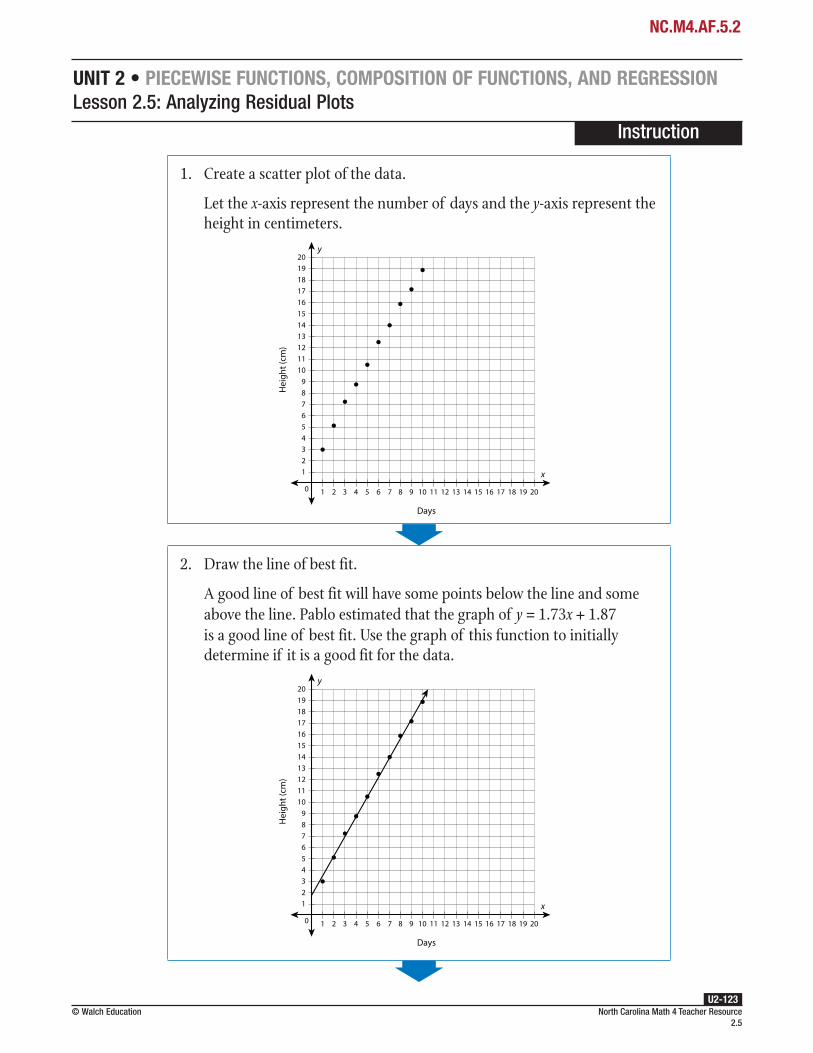
North Carolina Math 4 Teacher Resource 2.5
© Walch EducationU2-123
UNIT 2 • PIECEWISE FUNCTIONS, COMPOSITION OF FUNCTIONS, AND REGRESSIONLesson 2.5: Analyzing Residual Plots
Instruction
NC.M4.AF.5.2
1. Create a scatter plot of the data.
Let the x-axis represent the number of days and the y-axis represent the height in centimeters.
10 15 2051 4 62 3 7 8 9 11 12 13 14 16 17 18 190
y
13121110
987654321 x
Days
Hei
ght (
cm)
20191817161514
2. Draw the line of best fit.
A good line of best fit will have some points below the line and some above the line. Pablo estimated that the graph of y = 1.73x + 1.87 is a good line of best fit. Use the graph of this function to initially determine if it is a good fit for the data.
10 15 2051 4 62 3 7 8 9 11 12 13 14 16 17 18 190
y
13121110
987654321 x
Days
20191817161514
Hei
ght (
cm)

North Carolina Math 4 Teacher Resource 2.5
© Walch EducationU2-124
UNIT 2 • PIECEWISE FUNCTIONS, COMPOSITION OF FUNCTIONS, AND REGRESSIONLesson 2.5: Analyzing Residual Plots
Instruction
NC.M4.AF.5.2
3. Find the residuals for each data point.
The residual for each data point is the difference between the observed value and the estimated value using a line of best fit. Evaluate the function of the line at each value of x.
x y = 1.73x + 1.87
1 y = 1.73(1) + 1.87 = 3.6
2 y = 1.73(2) + 1.87 = 5.33
3 y = 1.73(3) + 1.87 = 7.06
4 y = 1.73(4) + 1.87 = 8.79
5 y = 1.73(5) + 1.87 = 10.52
6 y = 1.73(6) + 1.87 = 12.25
7 y = 1.73(7) + 1.87 = 13.98
8 y = 1.73(8) + 1.87 = 15.71
9 y = 1.73(9) + 1.87 = 17.44
10 y = 1.73(10) + 1.87 = 19.17
Next, find the difference between each observed value and each calculated value for each value of x.
x Residual
1 3 – 3.6 = –0.6
2 5.1 – 5.33 = –0.23
3 7.2 – 7.06 = 0.14
4 8.8 – 8.79 = 0.01
5 10.5 – 10.52 = –0.02
6 12.5 – 12.25 = 0.25
7 14 – 13.98 = 0.02
8 15.9 – 15.71 = 0.19
9 17.3 – 17.44 = –0.14
10 18.9 – 19.17 = –0.27

North Carolina Math 4 Teacher Resource 2.5
© Walch EducationU2-125
UNIT 2 • PIECEWISE FUNCTIONS, COMPOSITION OF FUNCTIONS, AND REGRESSIONLesson 2.5: Analyzing Residual Plots
Instruction
NC.M4.AF.5.2
4. Plot the residuals on a residual plot.
Plot the points (x, residual for x).
2 4 6 8 10
0.5
0.4
0.3
0.2
0.1
–0.1
–0.2
–0.3
–0.4
–0.5
–0.6
97531 11
–0.7
0
x
y
5. Describe the fit of the line based on the shape of the residual plot.
The plot of the residuals appears to be random, with some negative and some positive values. This indicates that the line is a good line of fit.
6. Use the equation to answer the question.
Use the equation to estimate the centimeters grown each day.
The change in the height per day is the centimeters grown each day. In the equation of the line, the slope is the change in height per day. The plant is growing approximately 1.73 centimeters each day.

North Carolina Math 4 Teacher Resource 2.5
© Walch EducationU2-126
UNIT 2 • PIECEWISE FUNCTIONS, COMPOSITION OF FUNCTIONS, AND REGRESSIONLesson 2.5: Analyzing Residual Plots
Instruction
NC.M4.AF.5.2
Example 2
Lindsay created the following table, which shows the population of fruit flies over the last 10 weeks.
Week Number of flies1 502 783 984 1225 1536 1917 2388 2989 373
10 466
She estimates that the population of fruit flies can be represented by the function y = 46x – 40. Using residuals, determine if her representation is a good estimate. If it is not a good estimate, find another function that could model the data.
1. Find the estimated population at each x-value.
Evaluate the function at each value of x.
x y = 46x – 401 46(1) – 40 = 62 46(2) – 40 = 523 46(3) – 40 = 984 46(4) – 40 = 1445 46(5) – 40 = 1906 46(6) – 40 = 2367 46(7) – 40 = 2828 46(8) – 40 = 3289 46(9) – 40 = 374
10 46(10) – 40 = 420

North Carolina Math 4 Teacher Resource 2.5
© Walch EducationU2-127
UNIT 2 • PIECEWISE FUNCTIONS, COMPOSITION OF FUNCTIONS, AND REGRESSIONLesson 2.5: Analyzing Residual Plots
Instruction
NC.M4.AF.5.2
2. Find the residuals by finding each difference between the observed population and estimated population.
x Residual1 50 – 6 = 442 78 – 52 = 263 98 – 98 = 04 122 – 144 = –225 153 – 190 = –376 191 – 236 = –457 238 – 282 = –448 298 – 328 = –309 373 – 374 = –1
10 466 – 420 = 46
3. Create a residual plot.
Plot the points (x, residual for x).
2 4 6 8 10
50
40
30
20
10
45
35
25
15
5
3 5 7 91 110
x
y
–20
–30
–40
–50
–15
–25
–35
–45
–5
–10

North Carolina Math 4 Teacher Resource 2.5
© Walch EducationU2-128
UNIT 2 • PIECEWISE FUNCTIONS, COMPOSITION OF FUNCTIONS, AND REGRESSIONLesson 2.5: Analyzing Residual Plots
Instruction
NC.M4.AF.5.2
4. Analyze the residual plot to determine if the function is a good estimate for the data.
The residual plot has a U-shape. This indicates that a non-linear estimation would be a better fit for this data set.
The shape of the residual plot indicates that the function y = 46x – 40 is not a good estimate for this data set.
5. Choose a different function model and use a calculator to fit it to the data.
First, decide which model type to use. As population growth often exhibits exponential growth, use an exponential model.
On a TI-83/84:
Step 1: Press [STAT] to bring up the statistics menu. The first option, 1: Edit, will already be highlighted. Press [ENTER].
Step 2: Arrow up to L1 and press [CLEAR], then [ENTER], to clear the list. Repeat this process to clear L2 and L3 if needed.
Step 3: Enter the ordered pairs in the L1 and L2 lists. Make sure to enter the x-coordinates in L1 and the y-coordinates in L2.
Step 4: Press [STAT]. Arrow to the CALC menu. Press 0: ExpReg.
Step 5: Press [(], then [2ND][1] to type “L1” for Xlist. Press [,], then [2ND][2] to type “L2” for Ylist. Press [)] to close the parentheses.
Step 6: Press [ENTER] to calculate.
(continued)
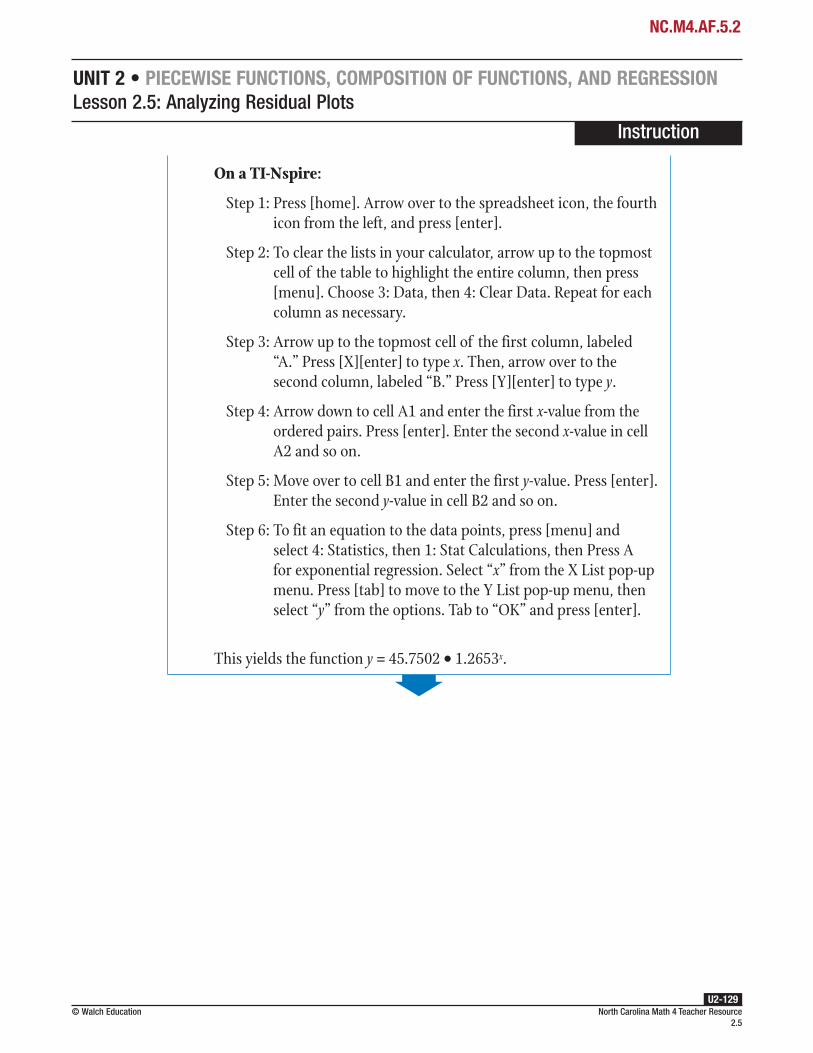
North Carolina Math 4 Teacher Resource 2.5
© Walch EducationU2-129
UNIT 2 • PIECEWISE FUNCTIONS, COMPOSITION OF FUNCTIONS, AND REGRESSIONLesson 2.5: Analyzing Residual Plots
Instruction
NC.M4.AF.5.2
On a TI-Nspire:
Step 1: Press [home]. Arrow over to the spreadsheet icon, the fourth icon from the left, and press [enter].
Step 2: To clear the lists in your calculator, arrow up to the topmost cell of the table to highlight the entire column, then press [menu]. Choose 3: Data, then 4: Clear Data. Repeat for each column as necessary.
Step 3: Arrow up to the topmost cell of the first column, labeled “A.” Press [X][enter] to type x. Then, arrow over to the second column, labeled “B.” Press [Y][enter] to type y.
Step 4: Arrow down to cell A1 and enter the first x-value from the ordered pairs. Press [enter]. Enter the second x-value in cell A2 and so on.
Step 5: Move over to cell B1 and enter the first y-value. Press [enter]. Enter the second y-value in cell B2 and so on.
Step 6: To fit an equation to the data points, press [menu] and select 4: Statistics, then 1: Stat Calculations, then Press A for exponential regression. Select “x” from the X List pop-up menu. Press [tab] to move to the Y List pop-up menu, then select “y” from the options. Tab to “OK” and press [enter].
This yields the function y = 45.7502 • 1.2653x.

North Carolina Math 4 Teacher Resource 2.5
© Walch EducationU2-130
UNIT 2 • PIECEWISE FUNCTIONS, COMPOSITION OF FUNCTIONS, AND REGRESSIONLesson 2.5: Analyzing Residual Plots
Instruction
NC.M4.AF.5.2
6. Graph the new function on a scatter plot of the data.
Create a table of values to graph the function.
Evaluate the function at each value of x.
x Actual Predicted y = 45.7502 • 1.2653x
1 50 45.7502 • 1.2653(1) ≈ 582 78 45.7502 • 1.2653(2) ≈ 733 98 45.7502 • 1.2653(3) ≈ 934 122 45.7502 • 1.2653(4) ≈ 1175 153 45.7502 • 1.2653(5) ≈ 1486 191 45.7502 • 1.2653(6) ≈ 1887 238 45.7502 • 1.2653(7) ≈ 2388 298 45.7502 • 1.2653(8) ≈ 3019 373 45.7502 • 1.2653(9) ≈ 380
10 466 45.7502 • 1.2653(10) ≈ 481
Plotted with the data points, the graph of y = 45.7502 • 1.2653x should resemble the following:
2 4 6 8 101 3 5 7 90
Weeks
320
240
260
80
200
120
40
280
400
440
360
File
s
480
x
y500
11
This function does indeed appear to be a good fit for the data.

North Carolina Math 4 Teacher Resource 2.5
© Walch EducationU2-131
UNIT 2 • PIECEWISE FUNCTIONS, COMPOSITION OF FUNCTIONS, AND REGRESSIONLesson 2.5: Analyzing Residual Plots
Instruction
NC.M4.AF.5.2
7. Create a residual plot for the new function.
Find the residuals for the new function, building on the table in the previous step.
x Actual Predicted Residual
1 50 58 50 – 58 = –8
2 78 73 78 – 73 = 5
3 98 93 98 – 93 = 5
4 122 117 122 – 117 = 5
5 153 148 153 – 148 = 5
6 191 188 191 – 188 = 3
7 238 238 238 – 238 = 0
8 298 301 298 – 301 = –3
9 373 380 373 – 380 = –7
10 466 481 466 – 481 = –15
Next, plot the points (x, residual for x).
–10
–20
20
10
0
y
2 4 6 8 100
x
While the residual plot is still U-shaped, the residuals are notably smaller than they were for the linear model.

North Carolina Math 4 Teacher Resource 2.5
© Walch EducationU2-132
UNIT 2 • PIECEWISE FUNCTIONS, COMPOSITION OF FUNCTIONS, AND REGRESSIONLesson 2.5: Analyzing Residual Plots
Instruction
NC.M4.AF.5.2
Example 3
Chelsea has been tracking the fuel economy of her car. She has noticed that the fuel economy (in miles per gallon) seems to vary with the average speed of the car. Her findings are summarized in the following table:
Average Speed (mph) Fuel Economy (mpg)
40 33.2
45 33.5
50 31.9
55 30.3
60 27.9
65 24.9
70 24.1
Chelsea determined that she could model this relationship with the function y = –0.0067x2 + 0.39x + 28.81. Use a residual plot to determine how well the function fits the data. What value would you expect the fuel economy to reach when the average speed is 35 mph?
1. Create a scatter plot of the data.
Let the x-axis represent the speed and the y-axis represent the fuel economy.
29
27
25
23
21
26
24
22
20
28
3940
37
35
33
31
36
34
32
30
38
40 50 60 7035 45 55 65 75
45y
x
Miles per hour
Mile
s pe
r gal
lon

North Carolina Math 4 Teacher Resource 2.5
© Walch EducationU2-133
UNIT 2 • PIECEWISE FUNCTIONS, COMPOSITION OF FUNCTIONS, AND REGRESSIONLesson 2.5: Analyzing Residual Plots
Instruction
NC.M4.AF.5.2
2. Graph the given function.
The function that Chelsea used to estimate the fuel economy is y = –0.0067x2 + 0.39x + 28.81. Create a table of values to graph the function.
Evaluate the function at each value of x.
x Actual Predicted y = –0.0067x2 + 0.39x + 28.81
40 33.2 –0.0067(40)2 + 0.39(40) + 28.81 ≈ 33.7
45 33.5 –0.0067(45)2 + 0.39(45) + 28.81 ≈ 32.8
50 31.9 –0.0067(50)2 + 0.39(50) + 28.81 ≈ 31.6
55 30.3 –0.0067(55)2 + 0.39(55) + 28.81 ≈ 30.0
60 27.9 –0.0067(60)2 + 0.39(60) + 28.81 ≈ 28.1
65 24.9 –0.0067(65)2 + 0.39(65) + 28.81 ≈ 25.9
70 24.1 –0.0067(70)2 + 0.39(70) + 28.81 ≈ 23.3
Plot the x, y points on the graph and connect them with a curve.
29
27
25
23
21
26
24
22
20
28
3940
37
35
33
31
36
34
32
30
38
40 50 60 7035 45 55 65 75
45y
x
Miles per hour
Mile
s pe
r gal
lon

North Carolina Math 4 Teacher Resource 2.5
© Walch EducationU2-134
UNIT 2 • PIECEWISE FUNCTIONS, COMPOSITION OF FUNCTIONS, AND REGRESSIONLesson 2.5: Analyzing Residual Plots
Instruction
NC.M4.AF.5.2
3. Find the residuals.
Find the difference between each observed fuel economy measurement and estimated fuel economy measurement.
x Actual Predicted Residual
40 33.2 33.7 33.2 – 33.7 = –0.5
45 33.5 32.8 33.5 – 32.8 = 0.7
50 31.9 31.6 31.9 – 31.6 = 0.3
55 30.3 30 30.3 – 30 = 0.3
60 27.9 28.1 27.9 – 28.1 = –0.2
65 24.9 25.9 24.9 – 25.9 = –1
70 24.1 23.3 24.1 – 23.3 = 0.8
4. Create a residual plot.
Plot the points (x, residual for x).
40 50 60 7035 45 55 65
y
x
–0.4
–0.8
–0.6
–1
–0.2
0.8
0.4
1
0.6
0.2
0
1.2
–1.2

North Carolina Math 4 Teacher Resource 2.5
© Walch EducationU2-135
UNIT 2 • PIECEWISE FUNCTIONS, COMPOSITION OF FUNCTIONS, AND REGRESSIONLesson 2.5: Analyzing Residual Plots
Instruction
NC.M4.AF.5.2
5. Determine if the function is a good estimate for the data.
The residual plot has a random shape. The function is a good estimate for the data.
6. Use the function to estimate the fuel economy when the speed is 35 mph.
In the fitted function, x represents the speed and y represents the fuel economy. Evaluate the function for x = 35 to estimate the mpg at 35 mph.
y = –0.0067(35)2 + 0.39(35) + 28.81 = 34.2525 Substitute 35 for x.
At a speed of 35 mph, Chelsea’s car has a fuel economy of about 34.3 mpg.

North Carolina Math 4 Teacher Resource 2.5
© Walch EducationU2-136
UNIT 2 • PIECEWISE FUNCTIONS, COMPOSITION OF FUNCTIONS, AND REGRESSIONLesson 2.5: Analyzing Residual Plots
Name: Date:NC.M4.AF.5.2
Problem-Based Task 2.5: Estimating Salaries, Part IIMarcy surveys 20 people who work at different software companies. She asks each person how many years he or she has worked, and what his or her salary was last year. Marcy’s results are in the following table.
What function best fits the data? What should Marcy’s salary be when she has 12 years of work experience?
Years of experience
Salary in dollars ($)
Years of experience
Salary in dollars ($)
1 53,000 5 98,000
1 55,000 6 101,000
1 50,000 6 92,000
2 62,000 7 115,000
3 81,000 8 125,000
4 77,000 9 145,000
4 76,000 10 149,000
5 107,000 11 179,000
5 80,000 13 210,000
5 99,000 15 229,000
What function best fits the data? What should Marcy’s salary be when she has 12 years of work experience? Justify your answer.
SMP 1 ✓ 2 ✓3 ✓ 4 ✓5 ✓ 6 ✓7 ✓ 8 ✓

North Carolina Math 4 Teacher Resource 2.5
© Walch EducationU2-137
UNIT 2 • PIECEWISE FUNCTIONS, COMPOSITION OF FUNCTIONS, AND REGRESSIONLesson 2.5: Analyzing Residual Plots
Name: Date:NC.M4.AF.5.2
Problem-Based Task 2.5: Estimating Salaries, Part II
Coachinga. Create a scatter plot of the data.
b. Find a linear function to model the data and plot it on the scatter plot.
c. Plot the residuals for the linear function.
d. Is the linear function a good fit for the data?
e. Find an exponential function to model the data and plot it on the scatter plot.
f. Plot the residuals for the exponential function.
g. Is the exponential function a good fit for the data?
h. Find a quadratic function to model the data and plot it on the scatter plot.
i. Plot the residuals for the quadratic function.
j. Is the quadratic function a good fit for the data?
k. Which function is the best fit for the data?
l. What should Marcy’s salary be when she has 12 years of work experience? Why?

North Carolina Math 4 Teacher Resource 2.5
© Walch EducationU2-138
UNIT 2 • PIECEWISE FUNCTIONS, COMPOSITION OF FUNCTIONS, AND REGRESSIONLesson 2.5: Analyzing Residual Plots
Instruction
NC.M4.AF.5.2
Problem-Based Task 2.5: Estimating Salaries, Part II
Coaching Sample Responsesa. Create a scatter plot of the data.
Let the x-axis represent years of experience and the y-axis represent salary.
2 4 6 8 101 3 5 7 9 12 1411 13 150 16
y
x
Years of experience
200,000
160,000
120,000
80,000
40,000
140,000
100,000
60,000
20,000
180,000
240,000
260,000
220,000
Sala
ry ($
)
280,000
17
b. Find a linear function to model the data and plot it on the scatter plot.
Use a calculator or other technology to fit a linear function.
On a TI-83/84:
Step 1: Press [STAT] to bring up the statistics menu. The first option, 1: Edit, will already be highlighted. Press [ENTER].
Step 2: Arrow up to L1 and press [CLEAR], then [ENTER], to clear the list. Repeat this process to clear L2 and L3 if needed.
Step 3: Enter the ordered pairs in the L1 and L2 lists. Make sure to enter the x-coordinates in L1 and the y-coordinates in L2.
Step 4: Press [STAT]. Arrow to the CALC menu. Press 4: LinReg.
Step 5: Press [(], then [2ND][1] to type “L1” for Xlist. Press [,], then [2ND][2] to type “L2” for Ylist. Press [)] to close the parentheses.
Step 6: Press [ENTER] to calculate.

North Carolina Math 4 Teacher Resource 2.5
© Walch EducationU2-139
UNIT 2 • PIECEWISE FUNCTIONS, COMPOSITION OF FUNCTIONS, AND REGRESSIONLesson 2.5: Analyzing Residual Plots
Instruction
NC.M4.AF.5.2
On a TI-Nspire:
Step 1: Press [home]. Arrow over to the spreadsheet icon, the fourth icon from the left, and press [enter].
Step 2: To clear the lists in your calculator, arrow up to the topmost cell of the table to highlight the entire column, then press [menu]. Choose 3: Data, then 4: Clear Data. Repeat for each column as necessary.
Step 3: Arrow up to the topmost cell of the first column, labeled “A.” Press [X][enter] to type x. Then, arrow over to the second column, labeled “B.” Press [Y][enter] to type y.
Step 4: Arrow down to cell A1 and enter the first x-value from the ordered pairs. Press [enter]. Enter the second x-value in cell A2 and so on.
Step 5: Move over to cell B1 and enter the first y-value. Press [enter]. Enter the second y-value in cell B2 and so on.
Step 6: To fit an equation to the data points, press [menu] and select 4: Statistics, then 1: Stat Calculations, then Press 3 for linear regression. Select “x” from the X List pop-up menu. Press [tab] to move to the Y List pop-up menu, then select “y” from the options. Tab to “OK” and press [enter].
The function is y = 12,601x + 32,914. The graph should resemble the following:
2 4 6 8 10
200,000
160,000
120,000
80,000
40,000
140,000
100,000
60,000
20,000
180,000
1 3 5 7 9 12 1411 13 15
240,000
260,000
220,000
0 16
y
x
Sala
ry ($
)
Years of experience
280,000
17

North Carolina Math 4 Teacher Resource 2.5
© Walch EducationU2-140
UNIT 2 • PIECEWISE FUNCTIONS, COMPOSITION OF FUNCTIONS, AND REGRESSIONLesson 2.5: Analyzing Residual Plots
Instruction
NC.M4.AF.5.2
c. Plot the residuals for the linear function.
Evaluate the function at each value of x, and subtract this value from each of the actual values to find the residuals.
Years of Experience Actual Salary Predicted Salary Residual
1 53,000 45,515 7,485
1 55,000 45,515 9,485
1 50,000 45,515 4,485
2 62,000 58,116 3,884
3 81,000 70,717 10,283
4 77,000 83,318 –6,318
4 76,000 83,318 –7,318
5 107,000 95,919 11,081
5 80,000 95,919 –15,919
5 99,000 95,919 3,081
5 98,000 95,919 2,081
6 101,000 108,520 –7,520
6 92,000 108,520 –16,520
7 115,000 121,121 –6,121
8 125,000 133,722 –8,722
9 145,000 146,323 –1,323
10 149,000 158,924 –9,924
11 179,000 171,525 7,475
13 210,000 196,727 13,273
15 229,000 221,929 7,071

North Carolina Math 4 Teacher Resource 2.5
© Walch EducationU2-141
UNIT 2 • PIECEWISE FUNCTIONS, COMPOSITION OF FUNCTIONS, AND REGRESSIONLesson 2.5: Analyzing Residual Plots
Instruction
NC.M4.AF.5.2
The plot should resemble the following:
2 4 6 8 101 3 5 7 9
–8,000
–16,000
–12,000
–4,000
16,000
8,000
12,000
4,000
0
y
x
11 12 13 14 15
d. Is the linear function a good fit for the data?
The residual plot has a U-shape. A linear function may not be the best fit for the data.
e. Find an exponential function to model the data and plot it on the scatter plot.
Use a calculator or other technology to fit an exponential function.
On a TI-83/84:
Step 1: Verify that the ordered pairs are entered into the L1 and L2 lists.
Step 2: Press [STAT]. Arrow to the CALC menu. Press 0: ExpReg.
Step 3: Press [(], then [2ND][1] to type “L1” for Xlist. Press [,], then [2ND][2] to type “L2” for Ylist. Press [)] to close the parentheses.
Step 4: Press [ENTER] to calculate.
On a TI-Nspire:
Step 1: Verify that the ordered pairs are entered into the x and y lists.
Step 2: To fit an equation to the data points, press [menu] and select 4: Statistics, then 1: Stat Calculations, then Press A for exponential regression. Select “x” from the X List pop-up menu. Press [tab] to move to the Y List pop-up menu, then select “y” from the options. Tab to “OK” and press [enter].

North Carolina Math 4 Teacher Resource 2.5
© Walch EducationU2-142
UNIT 2 • PIECEWISE FUNCTIONS, COMPOSITION OF FUNCTIONS, AND REGRESSIONLesson 2.5: Analyzing Residual Plots
Instruction
NC.M4.AF.5.2
The function is y = 51,471 • 1.1149x. The graph should resemble the following:
2 4 6 8 101 3 5 7 9 12 1411 13 150 16
y
x
Years of experience
200,000
160,000
120,000
80,000
40,000
140,000
100,000
60,000
20,000
180,000
240,000
260,000
220,000Sa
lary
($)
280,000
17
f. Plot the residuals for the exponential function.
Evaluate the function at each value of x, and subtract this value from each of the actual values to find the residuals.
Years of Experience Actual Salary Predicted Salary Residual
1 53,000 57,387 –4,387
1 55,000 57,387 –2,387
1 50,000 57,387 –7,387
2 62,000 63,983 –1,983
3 81,000 71,337 9,663
4 77,000 79,537 –2,537
4 76,000 79,537 –3,537
5 107,000 88,679 18,321
5 80,000 88,679 –8,679
5 99,000 88,679 10,321
5 98,000 88,679 9,321
(continued)

North Carolina Math 4 Teacher Resource 2.5
© Walch EducationU2-143
UNIT 2 • PIECEWISE FUNCTIONS, COMPOSITION OF FUNCTIONS, AND REGRESSIONLesson 2.5: Analyzing Residual Plots
Instruction
NC.M4.AF.5.2
Years of Experience Actual Salary Predicted Salary Residual
6 101,000 98,871 2,129
6 92,000 98,871 –6,871
7 115,000 110,235 4,765
8 125,000 122,906 2,094
9 145,000 137,033 7,967
10 149,000 152,783 –3,783
11 179,000 170,344 8,656
13 210,000 211,753 –1,753
15 229,000 263,227 –34,227
The plot should resemble the following:
2 4 6 8 101 3 5 7 9
–20,000
–40,000
–30,000
–10,000
40,000
20,000
30,000
10,000
0
y
x
11 12 13 14 15
–50,000
g. Is the exponential function a good fit for the data?
The residual plot has a U-shape, and the residuals are larger than they were for the linear function. An exponential function is not a good fit for the data.

North Carolina Math 4 Teacher Resource 2.5
© Walch EducationU2-144
UNIT 2 • PIECEWISE FUNCTIONS, COMPOSITION OF FUNCTIONS, AND REGRESSIONLesson 2.5: Analyzing Residual Plots
Instruction
NC.M4.AF.5.2
h. Find a quadratic function to model the data and plot it on the scatter plot.
Use a calculator or other technology to fit a quadratic function.
On a TI-83/84:
Step 1: Verify that the ordered pairs are entered into the L1 and L2 lists.
Step 2: Press [STAT]. Arrow to the CALC menu. Press 5: QuadReg.
Step 3: Press [(], then [2ND][1] to type “L1” for Xlist. Press [,], then [2ND][2] to type “L2” for Ylist. Press [)] to close the parentheses.
Step 4: Press [ENTER] to calculate.
On a TI-Nspire:
Step 1: Verify that the ordered pairs are entered into the x and y lists.
Step 2: To fit an equation to the data points, press [menu] and select 4: Statistics, then 1: Stat Calculations, then Press 6 for quadratic regression. Select “x” from the X List pop-up menu. Press [tab] to move to the Y List pop-up menu, then select “y” from the options. Tab to “OK” and press [enter].
The function is y = 325.16x2 + 7827.2x + 45,066. The graph should resemble the following:
2 4 6 8 101 3 5 7 9 12 1411 13 150 16
y
x
Years of experience
200,000
160,000
120,000
80,000
40,000
140,000
100,000
60,000
20,000
180,000
240,000
260,000
220,000
Sala
ry ($
)
280,000
17
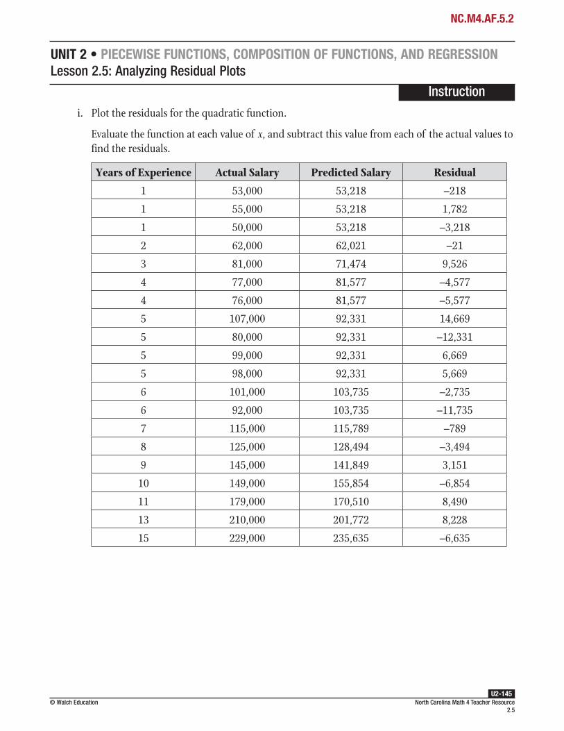
North Carolina Math 4 Teacher Resource 2.5
© Walch EducationU2-145
UNIT 2 • PIECEWISE FUNCTIONS, COMPOSITION OF FUNCTIONS, AND REGRESSIONLesson 2.5: Analyzing Residual Plots
Instruction
NC.M4.AF.5.2
i. Plot the residuals for the quadratic function.
Evaluate the function at each value of x, and subtract this value from each of the actual values to find the residuals.
Years of Experience Actual Salary Predicted Salary Residual
1 53,000 53,218 –218
1 55,000 53,218 1,782
1 50,000 53,218 –3,218
2 62,000 62,021 –21
3 81,000 71,474 9,526
4 77,000 81,577 –4,577
4 76,000 81,577 –5,577
5 107,000 92,331 14,669
5 80,000 92,331 –12,331
5 99,000 92,331 6,669
5 98,000 92,331 5,669
6 101,000 103,735 –2,735
6 92,000 103,735 –11,735
7 115,000 115,789 –789
8 125,000 128,494 –3,494
9 145,000 141,849 3,151
10 149,000 155,854 –6,854
11 179,000 170,510 8,490
13 210,000 201,772 8,228
15 229,000 235,635 –6,635

North Carolina Math 4 Teacher Resource 2.5
© Walch EducationU2-146
UNIT 2 • PIECEWISE FUNCTIONS, COMPOSITION OF FUNCTIONS, AND REGRESSIONLesson 2.5: Analyzing Residual Plots
Instruction
NC.M4.AF.5.2
The plot should resemble the following:
2 4 6 8 101 3 5 7 9
–8,000
–16,000
–12,000
–4,000
16,000
8,000
12,000
4,000
0
y
x
11 12 13 14 15
j. Is the quadratic function a good fit for the data?
The residual plot of the quadratic function has less of a U-shape and has smaller residuals than either the linear or the exponential models. A quadratic function is a good fit for the data.
k. Which function is the best fit for the data?
The quadratic function models the data best; the residuals are smallest for this function, and the residual plot has the least distinct pattern.
l. What should Marcy’s salary be when she has 12 years of work experience? Why?
Use the quadratic function to find the estimated salary after 12 years of work experience.
y = 325.16x2 + 7,827.2x + 45,066
y = 325.16(12)2 + 7,827.2(12) + 45,066
y = 325.16(144) + 7,827.2(12) + 45,066
y = 46,823.04 + 93,926.4 + 45,066
y = 185,815.44
Marcy’s salary should be about $189,000 after 12 years of work experience.
Recommended Closure Activity
Select one or more of the essential questions for a class discussion or as a journal entry prompt.

North Carolina Math 4 Teacher Resource 2.5
© Walch EducationU2-147
UNIT 2 • PIECEWISE FUNCTIONS, COMPOSITION OF FUNCTIONS, AND REGRESSIONLesson 2.5: Analyzing Residual Plots
Name: Date:NC.M4.AF.5.2
continued
APractice 2.5: Analyzing Residual PlotsTo understand the density of a deer population, Lewis counts the deer in different areas of a forest. He records the deer in each portion of the forest in a data table. Use the data for problems 1–4.
Acres of forest Deer population5 108 0
10 014 4220 10022 6630 9045 18050 10058 116
1. Create a scatter plot showing the deer population in each acreage.
2. Lewis states that the population can be estimated using the equation y = 2x + 22. Graph the equation on the scatter plot.
3. Does it appear that this line is a good fit for the data? Explain.

North Carolina Math 4 Teacher Resource 2.5
© Walch EducationU2-148
UNIT 2 • PIECEWISE FUNCTIONS, COMPOSITION OF FUNCTIONS, AND REGRESSIONLesson 2.5: Analyzing Residual Plots
Name: Date:NC.M4.AF.5.2
4. Use a residual plot to determine if a linear function is a good fit for the data.
Skylar has a savings account. She records the balance in the account each year. Use the data for problems 5–10.
Years Account balance in dollars ($)2 5513 5784 6085 6386 6707 7048 7399 776
5. Create a scatter plot of the account balances.
continued
x
y

North Carolina Math 4 Teacher Resource 2.5
© Walch EducationU2-149
UNIT 2 • PIECEWISE FUNCTIONS, COMPOSITION OF FUNCTIONS, AND REGRESSIONLesson 2.5: Analyzing Residual Plots
Name: Date:NC.M4.AF.5.2
6. Skylar estimates that the account balance can be represented by the equation y = 32x + 483. Draw the line of the equation on the scatter plot.
7. Does it appear that this line is a good fit for the data? Explain.
8. Use a residual plot to determine if a linear function is a good fit for the data.
x
y
9. Find another equation that fits the data and plot it on a scatter plot of the data.
continued

North Carolina Math 4 Teacher Resource 2.5
© Walch EducationU2-150
UNIT 2 • PIECEWISE FUNCTIONS, COMPOSITION OF FUNCTIONS, AND REGRESSIONLesson 2.5: Analyzing Residual Plots
Name: Date:NC.M4.AF.5.2
10. Use a residual plot to determine if this function is a good fit for the data.
x
y

North Carolina Math 4 Teacher Resource 2.5
© Walch EducationU2-151
UNIT 2 • PIECEWISE FUNCTIONS, COMPOSITION OF FUNCTIONS, AND REGRESSIONLesson 2.5: Analyzing Residual Plots
Name: Date:NC.M4.AF.5.2
continued
Practice 2.5: Analyzing Residual PlotsA ball is dropped from a height of 600 meters. The height of the ball is recorded as it falls. The data is shown in the following table. Use the data for problems 1–4.
Time in seconds Height in meters2 5813 5505 5066 4467 3878 3129 224
10 12212 10
1. Create a scatter plot showing the time and height of the ball.
2. Ian determines that the height of the ball can be estimated using the equation y = –3.61x2 – 9.99x + 622.83. Draw the line of the equation on the scatter plot.
3. Does it appear that this function is a good fit for the data?
B

North Carolina Math 4 Teacher Resource 2.5
© Walch EducationU2-152
UNIT 2 • PIECEWISE FUNCTIONS, COMPOSITION OF FUNCTIONS, AND REGRESSIONLesson 2.5: Analyzing Residual Plots
Name: Date:NC.M4.AF.5.2
continued
4. Use a residual plot to determine if the function is a good fit for the data.
x
y
Dr. Sanchez is a pediatrician. She tracks the age and height of each patient. The height data for one male child is in the following table. Use the data for problems 5–8.
Age in months Height in inches1 203 236 278 299 31
12 3215 34
5. Create a scatter plot showing the age and height of the child.

North Carolina Math 4 Teacher Resource 2.5
© Walch EducationU2-153
UNIT 2 • PIECEWISE FUNCTIONS, COMPOSITION OF FUNCTIONS, AND REGRESSIONLesson 2.5: Analyzing Residual Plots
Name: Date:NC.M4.AF.5.2
6. Dr. Sanchez determines that the height can be estimated using the equation y = x + 20. Draw the line of the equation on the scatter plot.
7. Does it appear that this line is a good fit for the data? Explain.
8. Use a residual plot to determine if a linear function is a good fit for the data.
x
y
continued

North Carolina Math 4 Teacher Resource 2.5
© Walch EducationU2-154
UNIT 2 • PIECEWISE FUNCTIONS, COMPOSITION OF FUNCTIONS, AND REGRESSIONLesson 2.5: Analyzing Residual Plots
Name: Date:NC.M4.AF.5.2
Each student in Mrs. Goldman’s class records his or her height and his or her arm span in the following table. Use the data for problems 9 and 10.
Height in inches Arm span in inches Height in inches Arm span in inches66 65.3 74 71.058 61.5 50 49.047 47.0 57 59.971 66.7 56 56.668 66.6 52 56.265 63.7 55 58.964 60.8
9. Create a scatter plot of the heights versus arm spans.
10. Mrs. Goldman determines that arm spans can be estimated using the equation y = 0.78x + 13. Use a residual plot to determine if a linear function is a good fit for the data.
x
y

UNIT 2 • PIECEWISE FUNCTIONS, COMPOSITION OF FUNCTIONS, AND REGRESSION
Answer Key8. Theefficiencyincreasesastheintensityapproaches–1.9. Theefficiencydecreasesastheintensityapproaches–1.10. A(i)approaches1asibecomesmorenegative.B(i)
increasesasibecomesmorepositive.
Practice 2.1 B: Piecewise, Step, and Absolute Value Functions, p. U2-30
1. Thetotalpiecewiserelationdoesnotassociateeachdomainvaluewithauniquefunctionvalue;e.g.,thefunctionsrepresentedbycurvesusingtheseriesof pointsA,B,and CandC,E,andFdonotshowthisone-to-onecorrespondence.
2. PointsA, B, and CandpointsC and Dcouldformapiecewisefunction;pointsC andDandpointsC, E, and Fcouldalsoformapiecewisefunction.
3. (80,250)4. Onefunctioncouldconsistof ABC andCD: ABCcould
defineaquadraticfunction,andCDcoulddefineanexponentialoralinearfunction.Anotherfunctioncouldconsistof CDandCEF:CDcoulddefineanexponentialoralinearfunction,andCEFcoulddefineaquadraticfunction.
5. Thedatarepresentsapiecewisefunctionbecauseforeachinterval,[–3,–1],[–1,1],and[1,3],theslopesof thelinearpiecesaredifferent.
6. a=17. a=1andb=2forallthreerestricteddomains8. pointsC1,C2,andC3couldformalinearfunctionoverthe
domain[0,6]becauseof itsconstantslope;C3,C4,andC5couldformaquadraticfunctionoverthedomain[6,19.5]becauseof itsdecreasingrateof changeoverthatinterval;C5andC6couldformalinearfunctionoverthedomain[19.5,27]becauseof itsconstantslope.
9. S1S2S3S4couldformalinearfunctionoverthedomain[0,18]becauseof itsconstantslope;S4S5S6couldformaquadraticfunctionoverthedomain[18,27]becauseof itsincreasingrateof changeoverthatinterval.
10. ProfitoccurswhenS(t)>C(t),whichisbetweent=25.5andt=27.
Lesson 2.1: Piecewise, Step, and Absolute Value Functions (NC.M4.AF.4.1, NC.M4.AF.4.2)
Warm-Up 2.1, p. U2-51. (2, )∞
2. f(x) =4
3. ( , 3)−∞ −
4. f x x( )4
5
17
5= +
5. [–3,2]
Scaffolded Practice 2.1: Piecewise, Step, and Absolute Value Functions, p. U2-11
1. pointsA,B,andCovertheinterval[–2,0]andpointsCandDovertheinterval[0,1]foracontinuousfunction;pointsA,B,andCovertheinterval[–2,0];andpointsDandEovertheinterval[1,2]foradiscontinuousfunction
2. pointsAandB overtheinterval[–2,–1)for y=0.0625;pointsBandCovertheinterval[–1,0)fory=0.25;pointsCandDovertheinterval[1,2]fory=1;andpointsD andEovertheinterval[1,2]fory=0.5foracontinuousfunction
3. pointsA,B,andCandpointsC,D,andEovertheinterval[–2,2]
4. f(x)andg(x)5. g(x)andh(x)6. f(x)andh(x)7. combinationfunction8. absolutevalueinequality9. combinationfunction10. combinationfunction
Practice 2.1 A: Piecewise, Step, and Absolute Value Functions, p. U2-27
1. Thefunctionpiecesovertheinterval(0,105)and(7•105,8•105)arelinearfunctions;thefunctionpieceovertheinterval[105,7•105]isaconstantfunction,T(H)=100.
2. T(H)=0.0006•H+40overtheinterval(0,105).3. T(H)=100overtheinterval[105,7•105].4. T(H)=0.0006•H –320overtheinterval(7•105,8•105).5. Betweenthevaluesof tatwhichthefunctionisundefined,
thestepsof V(t)=4andV(t)=–4indicateaconstantvalueovertheirrespectiveintervals.
6. If thepatternof thefunctionvaluescontinuesforvaluesof tgreaterthanπ,thenthefunction’speriodisπ.
7. Thefunction V tt
t( )
4 • sin2
sin2= isequaltoeither4or–4
forallt,exceptwhent=2
π,π,orintegermultiplesof
thosevalues.
Lesson 2.2: Composition of Functions (NC.M4.AF.1.1)
Warm-Up 2.2, p. U2-331. g(x)=100x+2002. P(x)=g(x)–f(x)3. P(x)=55x +180.If Monicasells24lampsonline,shewill
earnaprofitof $1,500.
North Carolina Math 4 Teacher Resource Answer Key
© Walch EducationU2-155

Scaffolded Practice 2.2: Composition of Functions, p. U2-37
1. f g x( )( )2. g f x( )( )3. f g x x( ) 1( ) = −
4. g f x x( ) 1( ) = −
5. f g x x( ) 2 1( ) = +
6. g f x x( ) 2 1( ) = +
7. g f x x( ) 3 32( )= +
8. f g x x( ) 9 12( )= +
9. f g x x( ) 3( ) = −
10. 3, )∞
Practice 2.2 A: Composition of Functions, p. U2-521. 5 1x −2. 5 1x −3. 25x4. Thedomainof f(x)isallrealnumbersgreaterthanorequal
to1,or[1,∞),becausetherecannotbeanegativevalueundertheradicalsign.
5. Therangeof f(x)isallrealnumbersgreaterthanorequalto0,or[0,∞),becausethesmallestoutputvaluewillbe0.
6. Thedomainof f(g(x))canbefoundfindingthedomain
of g(x)andthedomainof thecompositionfunction.The
domainof g(x)isallrealnumbers.Thedomainof the
compositionfunctionf(g(x))is1
5,∞
.Theintersectionof
thesetwodomainsis1
5,∞
.
7. Thedomainof g(f(x))canbefoundbyfindingthedomainof f(x)andthedomainof thecompositionfunction.Setthevalueundertheradicalgreaterthanorequalto0andsolveforx.Inbothinstances,thisyieldsx≥1.Thedomainof g(f(x))is[1,∞).
8. Therearenorestrictionsonthedomainandrangeof g(g(x)).Therefore,thedomainandrangeareallrealnumbers.
9. C(S(p))=0.9p–50;S(C(p))=0.9p–4510. Substitute1,000forpinbothcompositionfunctionsto
yieldC(S(p))=$850andS(C(p))=$855.Taking10%off of thepricefirstandthenusingthecouponwillresultinthebetterdeal,withasavingsof $5overtheotheroptionof usingthecouponfirstandthenusingthe10%discount.
Practice 2.2 B: Composition of Functions, p. U2-541. 2x2+13x+202. 2x2–3x+43. 8x4–24x3+12x2+9x4. x+85. Thedomainandrangeareallrealnumbers.6. Thedomainandrangeareallrealnumbers.7. f(x)=x+58. g(x)=1.07x9. Thecompositionfunctionf(g(x))meansthatthe7%will
beappliedtotheoriginalscoreandthen5pointswillbeaddedtothatnewscore.
10. Thecompositionfunctiong(f(x))meansthatthe5pointswillbeaddedtotheoriginalscoreandthenthe7%increasewillbeappliedtothatnewscore.
Lesson 2.3: Evaluating Composite Functions in Various Forms (NC.M4.AF.1.2)
Warm-Up 2.3, p. U2-561. g(x)=1.07x2. g(f(x))3. $26.75
Scaffolded Practice 2.3: Evaluating Composite Functions in Various Forms, p. U2-60
1. 7282. 263. 54. 25. 0.56. 37. f(x)=0.85x8. g(x)=x–509. Firstapplyf(x),thenapplyg(x).10.Theorderdoesmatter;f(g(x))=0.85x–42.5,whereas
g(f(x))=0.85x–50.
Practice 2.3 A: Evaluating Composite Functions in Various Forms, p. U2-77
1. 42. –53. 54. 15. –4
6. 07. $508. $1509. 0.1110.4.56
Practice 2.3 B: Evaluating Composite Functions in Various Forms, p. U2-79
1. 22. 23. 84. 85. 2
6. about3.67. f(x)=0.8x8. $3609. 3.2110.0
North Carolina Math 4 Teacher Resource Answer Key
© Walch EducationU2-156

7.
2 4 6 8 100 1 3 5 7 9 12 1411 13 15
10
8
6
4
2
7
5
3
1
9
14
12
15
13
11
x–1
–1
y
8.
2 4 6 8 100 1 3 5 7 9 12 1411 13 15
10
8
6
4
2
7
5
3
1
9
14
12
15
13
11
x–1
–1
y
9.
2 4 6 8 100 1 3 5 7 9 12 1411 13 15
10
8
6
4
2
7
5
3
1
9
14
12
15
13
11
x–1
–1
y
Lesson 2.4: Linear, Exponential, and Quadratic Regression (NC.M4.AF.5.1)
Warm-Up 2.4, p. U2-811.
90
50
10
120
70
30
0
y
x
2 43 5 61Year
Am
ount
spe
nt ($
)
110
60
20
130
80
40
100
2. Thepointsdon’tseemtoformadistinctshape,buttheydoseemtoincreaseapproximatelylinearlyoverthefiveyears.
3.
90
50
10
120
70
30
0
y
x
2 43 5 61Year
Am
ount
spe
nt ($
)
110
60
20
130
80
40
100
Accordingtothegraph,$110isareasonableestimate.Withoutmoredata,itisdifficulttosayhowaccuratetheestimateis.
Scaffolded Practice 2.4: Linear, Exponential, and Quadratic Regression, p. U2-87
1. quadratic2. exponential3. linear4. y=–1.26x+15.735. y=0.43•1.72x6. y=0.74x2–6.39x+14.73
North Carolina Math 4 Teacher Resource Answer Key
© Walch EducationU2-157

4. y=1.58•1.2969x;thelinearfunctionappearstobethebetterfit.
3 3.4 3.8
4.2
3.8
3.4
4.4
4
3.6
3.22.8 3.2 3.6 4
x
Blossom width
Blos
som
hei
ght
y
5.
2 4 6 8 10
1,000,000
800,000
600,000
400,000
200,000
700,000
500,000
300,000
100,000
0
900,000
1 3 5 7 9 1211
1,400,000
1,200,000
1,300,000
1,100,000
Year
Popu
latio
n
y
x
6. Thedatafollowsadistinctcurve,soaquadraticorexponentialmodelisbetter.Populationgrowthisoftenexponential;useanexponentialmodel.
10.Answersmayvary.Ingeneral,thequadraticfunctionmightbethebestfitbecauseitseemstofollowtheshapeof thedatathebest,butthelinearfunctionandtheexponentialfunctionalsoseemtomodelthedatafairlywell.
Practice 2.4 A: Linear, Exponential, and Quadratic Regression, p. U2-106
1.
3 3.4 3.8
4.2
3.8
3.4
4.4
4
3.6
3.22.8 3.2 3.6 4
x
Blossom width
Blos
som
hei
ght
y
2. Thedatadoesn’tseemtocurve,andthecontextdoesn’tseemtosuggestaquadraticorexponentialrelationship.Alinearmodelisagoodfit.
3. y=0.98x+0.49
3 3.4 3.8
4.2
3.8
3.4
4.4
4
3.6
3.22.8 3.2 3.6 4
x
Blossom width
Blos
som
hei
ght
y
North Carolina Math 4 Teacher Resource Answer Key
© Walch EducationU2-158

Practice 2.4 B: Linear, Exponential, and Quadratic Regression, p. U2-109
1.
2.4 2.82.2 2.6 3
12
8
4
14
10
6
2
0
y
x
3.2 3.42
Diameter (in)
Wei
ght (
oz)
2. Answersmayvary;alinearfunctioncouldbeagoodfit,becausethedatalooksapproximatelylinear.However,anexponentialorquadraticfunctioncouldbeabetterfit,becausethedatalooksasif itcouldpossiblyhaveaslightcurve.Also,contextsuggeststhataquadraticfunctionmaybethebestfitbecauseweightisrelatedtovolume,whichisrelatedtothediameterthroughacubepower.
3. y=8.24x–14.28
2.4 2.82.2 2.6 3
12
8
4
14
10
6
2
0
y
x
3.2 3.42
Diameter (in)
Wei
ght (
oz)
7. y=18,397.4•1.38x;thefunctionisagoodfit.
2 4 6 8 10
1,000,000
800,000
600,000
400,000
200,000
700,000
500,000
300,000
100,000
0
900,000
1 3 5 7 9 1211
1,400,000
1,200,000
1,300,000
1,100,000
Year
Popu
latio
n
y
x
8. Thegraphcurvesupandthenbackdown;aquadraticmodelisthebestfit.
9. y=–0.51x2+17.8x+434.71;thefunctionisagoodfit.
600
400
200
700
500
300
100
0 4 82 6 10
x
12 1614 18 20 24 2822 26
y
Angle (°)
Dis
tanc
e (ft
)
10.about589feet
North Carolina Math 4 Teacher Resource Answer Key
© Walch EducationU2-159

4. y=2.77x2–7.06x+5.97;thequadraticfunctionisabetterfit.
2.4 2.82.2 2.6 3
12
8
4
14
10
6
2
0
y
x
3.2 3.42
Diameter (in)
Wei
ght (
oz)
5.
4 86 10
44,000
28,000
12,000
52,000
36,000
20,000
4,000
0
y
x
122
Age
Pric
e ($
)
48,000
32,000
16,000
56,000
40,000
24,000
8,000
6. Thedataiscurved,soaquadraticorexponentialfunctionisbest.Vehiclestendtoloseafixedpercentageof valueastheyage,somostlikelyanexponentialmodelisbetter.
7. y=44285.43•0.88x;thefunctionisagoodfit.
4 86 10
44,000
28,000
12,000
52,000
36,000
20,000
4,000
0
y
x
122
Age
Pric
e ($
)
48,000
32,000
16,000
56,000
40,000
24,000
8,000
8. Thedatadoesn’tseemtohaveacurve,andthecontextdoesn’tsuggestanon-linearmodel.Alinearfunctionisagoodfit.
9. y=3.95x+7.62;thefunctionisagoodfit.
4.4 4.84.2 4.6 5
28
26
24
29
27
25
23
y
x
5.2 5.44
Width (cm)
Leng
th (c
m)
22
10.about4.4cm
North Carolina Math 4 Teacher Resource Answer Key
© Walch EducationU2-160

2.
0
x
y
1 2 3 4 5 6 7 8 9 10
1
3
4
5
6
7
8
9
2
Hours worked
Hou
ses
visi
ted
10
11
12
11
3. yes
4. Itisagoodfitforthedata.
4 8 9 12
2
3
1
–1
–2
–3
6 10 1120
x
y
3 751
5.
0
x
y
2 4 6 8 10 12 14 16 18 20
4
12
8
Age in months
Leng
th in
inch
es
32
22 24 26 28 30 32 34 36
16
20
24
28
36
Lesson 2.5: Analyzing Residual Plots (NC.M4.AF.5.2)
Warm-Up 2.5, p. U2-1121.
2 4 6 8 10
10
9
8
7
6
5
4
3
2
1
1 3 5 7 90
x
y
2. Thedistanceistheabsolutevalueofthedifferencebetweenthetwoy-values:|6–4|=2.
3.
1 2 3 4 5
5
–1
–2
–3
–4
4
3
2
1
0
y
x
–5
–1–2–3–4–5
Scaffolded Practice 2.5: Analyzing Residual Plots, p. U2-118
1.
0
x
y
1 2 3 4 5 6 7 8 9 10
1
3
4
5
6
7
8
9
2
Hours worked
Hou
ses
visi
ted
10
11
12
11
North Carolina Math 4 Teacher Resource Answer Key
© Walch EducationU2-161

8. Theresidualplothasnoparticularpattern.Thefunctionisagoodfitforthedata.
2 4 6 8 101 3 5 7 9
–8
–16
–12
–20
–4
16
8
20
12
4
0
y
x
0
9.
0
x
y
2 4 6 8 10 12 14 16 18 20
5
10
Diameter
Piec
es o
f pep
pero
ni
35
22 24
15
20
25
30
50
50
40
45
10.Alinearfunctionisnotagoodfitforthedata.
8 16 18 24
4
6
2
–2
–4
–6
12 20 2240
x
y
6 14102
6. Theresidualplothasnoparticularpattern.Thefunctionisagoodfitforthedata.
6 10 14 18 304 8 12 16 26
–0.4
–0.8
–0.6
–1
–0.2
0.8
0.4
1
0.6
0.2
0
y
x
282420 22 32 34
7.
2 4 6 8 101 3 5 7 9
Days
Case
s
x
y
110
40
0
20
80
100
60
120
140
160
North Carolina Math 4 Teacher Resource Answer Key
© Walch EducationU2-162

5.
2 4 6 8 10
800
700
600
500
400
450
300
200
100
0
x
y
Years
Acc
ount
bal
ance
in d
olla
rs ($
)
1 3 5 7 9
750
650
550
350
250
150
50
6.
2 4 6 8 10
800
700
600
500
400
450
300
200
100
0
x
y
Years
Acc
ount
bal
ance
in d
olla
rs ($
)
1 3 5 7 9
750
650
550
350
250
150
50
7. Yes;thelineappearstofollowtheshapeofthedata.8. Thoughitappearedthatthelinefitthedata,theU-shape
oftheresidualplotindicatesthatalinearfunctionisnotagoodfitforthedata.
10
8
6
4
2
–2
–4
–6
–8
–10
5 102 31 4 6 7 8 9
x
y
0
9
7
5
3
1
–1
–3
–5
–7
–9
Practice 2.5 A: Analyzing Residual Plots, p. U2-1471.
10 20 30 40 50 60
120
110
100
90
80
70
60
50
40
30
20
10
x
y
Acres
Dee
r
5 15 25 35 45 55
115
105
95
85
75
65
55
45
35
25
15
0
5
2.
10 20 30 40 50 60
120
110
100
90
80
70
60
50
40
30
20
10
x
y
Acres
Dee
r
5 15 25 35 45 55
115
105
95
85
75
65
55
45
35
25
15
0
5
y = 2x + 22
3. Yes;itfollowstheshapeofthedata.4. Theplotappearsrandom,soalinearfunctionislikelya
goodfitforthedata.
10 20 30 40 50
50
40
30
20
10
45
35
25
15
5
15 25 35 455 550
x
y
–20
–30
–40
–15
–25
–35
–45
–5
–10
70
60
65
55
60
North Carolina Math 4 Teacher Resource Answer Key
© Walch EducationU2-163

2.
2 4 6 8 101 3 5 7 9
x
y
0 11 12
Hei
ght i
n m
eter
s
Time in seconds
200
100
400
500
300
600
700
800
13
3. Yes;itfollowstheshapeof thedata.4. Theplotappearsrandom,sothequadraticfunctionis
likelyagoodfitforthedata.
2 4 6 8 10 12
–20
–40
–30
–50
–10
40
20
50
30
10
0
y
x
5.
10 1551 4 62 3 7 8 9 11 12 13 14 160
y
x
Age in months
Hei
ght i
n in
ches
10
2468
12141618
2224
20
262830323436
9. y=499.39•1.05x
2 4 6 8 101 3 5 7 9
Years
Acc
ount
bal
ance
($)
x
y
200
0
100
400
500
300
600
700
800
10. Theresidualplotisrandom.Thefunctionisagoodfit.
2 4 6 8 101 3 5 7 9
–0.2
–0.4
–0.3
–0.5
–0.1
0.7
0.5
0.8
0.6
0.4
0
y
x
0.2
0.3
0.1
–0.7
–0.6
–0.8
Practice 2.5 B: Analyzing Residual Plots, p. U2-1511.
20 4 6 8 10 12 14
450
420
390360
330
300
270
240
210180
150
120
90
60
30 x
y
Time in seconds
Hei
ght i
n m
eter
s
1 3 5 7 9 11 13 15
600
570540
510
480
North Carolina Math 4 Teacher Resource Answer Key
© Walch EducationU2-164

9.
10 20 30 40 50 60 70
75
70
65
60
55
50
45
40
35
30
25
20
15
10
5
55 65 755 15 25 35 450
x
y
Height in inches
Arm
spa
n in
inch
es
10. Theresidualplotisrandom,soalinearfunctionisagoodfit.
0
x
y
4
3
2
1
5
–1
–2
–3
–4
–5
5020 3010 40 60 70 804515 255 35 55 65 75
6.
10 1551 4 62 3 7 8 9 11 12 13 14 160
y
x
Age in months
Hei
ght i
n in
ches
10
2468
12141618
2224
20
262830323436
7. Yes;itfollowstheshapeofthedataset.8. Whenlookingattheresidualplot,theshapeappearstobe
aU.Alinearfunctionisnotagoodfitforthedata.
0
x
y
4
3
2
1
5
–1
–2
–3
–4
–5
104 62 8 12 14 1693 51 7 11 13 15
North Carolina Math 4 Teacher Resource Answer Key
© Walch EducationU2-165


North Carolina Math 4 Teacher Resource Unit 2 Mid-Unit Assessment
© Walch EducationMA-1
UNIT 2 • PIECEWISE FUNCTIONS, COMPOSITION OF FUNCTIONS, AND REGRESSIONMid-Unit Assessment
Assessment
Name: Date:
Unit 2 Mid-Unit AssessmentCircle the letter of the best answer.
1. An absolute value function has the general form ( )f x x a b= − + . What is the specific function if f(0) = 0 and f(1) = –1?
a. ( ) 3 3f x x= − +
b. ( ) 3 3f x x= + +
c. ( ) 3 3f x x= + −
d. ( ) 3 3f x x= − −
2. What function model was composed with a step function to produce the following graph?
1 2 3
10
8
6
4
2
0 0.5 1.5 2.5
y
18
16
14
12
x
3.5 4.54
a. linear
b. quadratic
c. exponential
d. square root
continued

North Carolina Math 4 Teacher Resource Unit 2 Mid-Unit Assessment
© Walch EducationMA-2
UNIT 2 • PIECEWISE FUNCTIONS, COMPOSITION OF FUNCTIONS, AND REGRESSIONMid-Unit Assessment
Assessment
Name: Date:
3. The following graph models the shoreline above a particular beach. What function model(s) make up this graph?
10 20 30 40 50
10
8
6
4
2
7
5
3
1
0
9
5 15 25 35 45
y
60 70 80 9055 65 75 85
18
16
14
12
17
15
13
11
x
Distance from beach (meters)
Hei
ght a
bove
bea
ch (m
eter
s)
a. radical; piecewise
b. quadratic; piecewise
c. quadratic; radical; piecewise
d. quadratic; radical; linear
continued

North Carolina Math 4 Teacher Resource Unit 2 Mid-Unit Assessment
© Walch EducationMA-3
UNIT 2 • PIECEWISE FUNCTIONS, COMPOSITION OF FUNCTIONS, AND REGRESSIONMid-Unit Assessment
Assessment
Name: Date:
4. A new, simplified income tax bracket is proposed. In this proposed tax bracket, the first $10,000 is not taxed. Each dollar over $10,000 but under $50,000 is taxed at 12%. Each dollar over $50,000 but under $150,000 is taxed at 24%. Each dollar over $150,000 is taxed at 30%. Which function represents the taxed owed under this proposal?
a. ( )
0; 0 10, 0000.12( 10, 000); 10, 000 50, 000
0.24( 50, 000) 4, 800; 50, 000 150, 000
0.30( 150, 000) 28, 800; 150, 000
f x
xx x
x x
x x
=
≤ ≤− < ≤− + < ≤− + ≥
b. ( )
0; 0 10, 000
0.12 ; 10, 000 50, 000
0.24 ; 50, 000 150, 000
0.30 ; 150, 000
f x
xx x
x x
x x
=
≤ ≤< ≤< ≤
≥
c. ( )
0; 0 10, 000
0.12 ; 10, 000 50, 000
0.24 4, 800; 50, 000 150, 000
0.30 28, 800; 150, 000
f x
xx x
x x
x x
=
≤ ≤< ≤
+ < ≤+ ≥
d. ( )
0; 0 10, 000
12 ; 10, 000 50, 000
24 ; 50, 000 150, 000
30 ; 150, 000
f x
xx x
x x
x x
=
≤ ≤< ≤< ≤
≥
continued
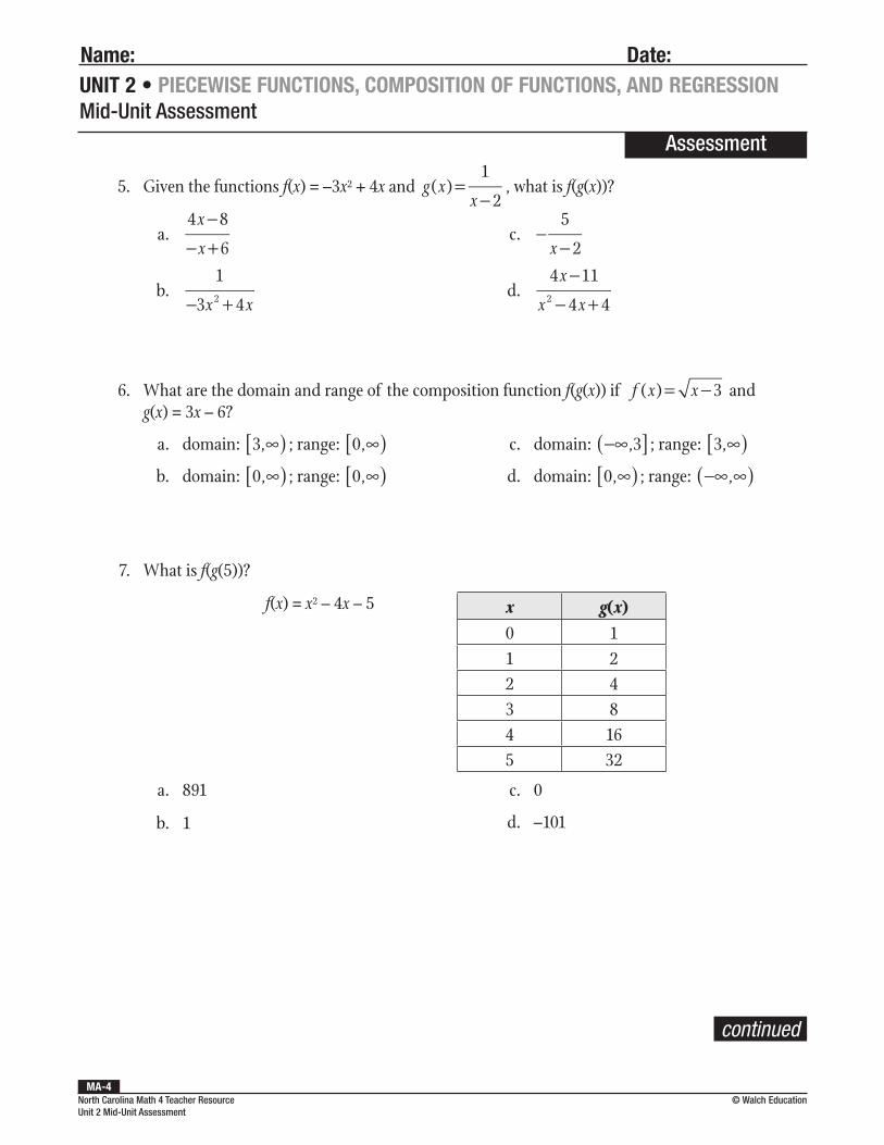
North Carolina Math 4 Teacher Resource Unit 2 Mid-Unit Assessment
© Walch EducationMA-4
UNIT 2 • PIECEWISE FUNCTIONS, COMPOSITION OF FUNCTIONS, AND REGRESSIONMid-Unit Assessment
Assessment
Name: Date:
5. Given the functions f(x) = –3x2 + 4x and ( )1
2g x
x=
−, what is f(g(x))?
a. 4 8
6
x
x
−− +
b. 1
3 42x x− +
c. 5
2x−
−
d. 4 11
4 42
x
x x
−− +
6. What are the domain and range of the composition function f(g(x)) if ( ) 3f x x= − and g(x) = 3x – 6?
a. domain: 3,[ )∞ ; range: 0,[ )∞
b. domain: 0,[ )∞ ; range: 0,[ )∞
c. domain: ,3](−∞ ; range: 3,[ )∞
d. domain: 0,[ )∞ ; range: ,( )−∞ ∞
7. What is f(g(5))?
f(x) = x2 – 4x – 5 x g(x) 0 11 22 43 84 165 32
a. 891
b. 1
c. 0
d. –101
continued

North Carolina Math 4 Teacher Resource Unit 2 Mid-Unit Assessment
© Walch EducationMA-5
UNIT 2 • PIECEWISE FUNCTIONS, COMPOSITION OF FUNCTIONS, AND REGRESSIONMid-Unit Assessment
Assessment
Name: Date:
8. What is g(f(0))?
x f(x)
0 10
1 9.5
2 9
3 8.5
4 8
5 7.52 4 6 8 10
10
1 3 5 7 9
–2
–4
–6
–8
8
6
4
2
0
y
x
–10
–1–2–3–4–5–6–7–8–9–10
g(x)
a. 8.5
b. 10
c. 3
d. 7
continued

North Carolina Math 4 Teacher Resource Unit 2 Mid-Unit Assessment
© Walch EducationMA-6
UNIT 2 • PIECEWISE FUNCTIONS, COMPOSITION OF FUNCTIONS, AND REGRESSIONMid-Unit Assessment
Assessment
Name: Date:
9. Let f(x) = 2 sin (πx) and g(x) = 2 • 0.5x. Which graph shows g(f(2))?
a.
(2, 2)
2 4 6 8 10
10
1 3 5 7 9
–2
–4
–6
–8
8
6
4
2
0
y
x
–10
–1–2–3–4–5–6–7–8–9–10
b.
(2, 2)
2 4 6 8 10
10
1 3 5 7 9
–2
–4
–6
–8
8
6
4
2
0
y
x
–10
–1–2–3–4–5–6–7–8–9–10
c.
(2, 0)2 4 6 8 10
10
1 3 5 7 9
–2
–4
–6
–8
8
6
4
2
0
y
x
–10
–1–2–3–4–5–6–7–8–9–10
d.
2 4 6 8 10
10
1 3 5 7 9
–2
–4
–6
–8
8
6
4
2
0
y
x
–10
–1–2–3–4–5–6–7–8–9–10
(2, 0.5)
continued

North Carolina Math 4 Teacher Resource Unit 2 Mid-Unit Assessment
© Walch EducationMA-7
UNIT 2 • PIECEWISE FUNCTIONS, COMPOSITION OF FUNCTIONS, AND REGRESSIONMid-Unit Assessment
Assessment
Name: Date:
Use the given information to complete all parts of problem 10.
10. A family data plan costs $50 per month. If all the data is used, additional data is automatically
added to the family account 10 gigabytes at a time, for a fee. Each additional 10 gigabytes
costs $10. The total billed to the family account can be modeled using the ceiling function
( ) 50 1010
P xx
= +
, where x is the number of gigabytes the family used over the plan
amount. The following graph depicts this function.
40 80
100
80
60
40
20
20 60 100
y
x
Bill
tota
l ($)
Data over plan (gigabytes)
0
a. How much would the family be charged if they were over plan by 14.2 gigabytes?
b. If the family account was billed $100 one month, how much data was used?
c. Write a piecewise function that gives the same values as P(x) over the interval [0, 60). Be sure to include domain restrictions for each piece.

North Carolina Math 4 Teacher Resource Unit 2 Mid-Unit Assessment
© Walch EducationMA-8
UNIT 2 • PIECEWISE FUNCTIONS, COMPOSITION OF FUNCTIONS, AND REGRESSIONMid-Unit Assessment
Instruction
Unit 2 Mid-Unit Assessment Answer KeyMultiple Choice
Answer Standard(s)
1. d NC.M4.AF.4.1
2. c NC.M4.AF.4.1
3. c NC.M4.AF.4.2
4. a NC.M4.AF.4.2
5. d NC.M4.AF.1.1
6. a NC.M4.AF.1.1
7. a NC.M4.AF.1.2
8. c NC.M4.AF.1.2
9. b NC.M4.AF.1.2
Extended Response
Answer Standard(s)
10. a. $70
b. at least 40 gigabytes but less than 50 gigabytes
c. ( )
10; 0 1020; 10 20
30; 20 30
40; 30 40
50; 40 50
60; 50 60
f x
xx
x
x
x
x
=
≤ <≤ <≤ <≤ <≤ <≤ <
NC.M4.AF.4.1, NC.M4.AF.4.2

North Carolina Math 4 Teacher Resource Unit 2 End-of-Unit Assessment
© Walch EducationEA-1
UNIT 2 • PIECEWISE FUNCTIONS, COMPOSITION OF FUNCTIONS, AND REGRESSIONEnd-of-Unit Assessment
Assessment
Name: Date:
Unit 2 End-of-Unit Assessment
Circle the letter of the best answer.
1. Which function matches the following graph?
2 4 6 8 10
10
1 3 5 7 9
–2
–4
–6
–8
8
6
4
2
0
y
x
–10
–1–2–3–4–5–6–7–8–9–10
a. ( ) 5f x x= −
b. ( ) 5f x x x= + +
c. ( ) 5f x x= +
d. ( ) 5f x x x= + −
continued

North Carolina Math 4 Teacher Resource Unit 2 End-of-Unit Assessment
© Walch EducationEA-2
UNIT 2 • PIECEWISE FUNCTIONS, COMPOSITION OF FUNCTIONS, AND REGRESSIONEnd-of-Unit Assessment
Assessment
Name: Date:
2. Reina is distributing crayons to her five young cousins. Each child will get an equal number of
crayons. The number of crayons distributed is represented in the graph of ( )5
f xx
=
. What
piecewise function has the same graph over the domain [10, 20)?
10 20 30 40 50
10
8
6
4
2
7
5
3
1
0
9
5 15 25 35 45
y
60 70 80 9055 65 75 85
18
16
14
12
17
15
13
11
x
Total number of crayons
Cray
ons
per c
hild
95
19
a. ( )2; 10 15
3; 15 20f x
xx
=≤ <≤ <
b. ( )
2; 10 15
3; 15 20
4; 20
f x
xx
x=
≤ <≤ <=
c. ( )
1; 10
2; 10 15
3; 15 20
f x
x
x
x
==< << <
d. ( )2; 10 153; 15 20
f xxx
=< << <
continued

North Carolina Math 4 Teacher Resource Unit 2 End-of-Unit Assessment
© Walch EducationEA-3
UNIT 2 • PIECEWISE FUNCTIONS, COMPOSITION OF FUNCTIONS, AND REGRESSIONEnd-of-Unit Assessment
Assessment
Name: Date:
3. When you start to drag a concrete block across a flat surface, two types of friction will act on the block: static friction, which prevents the block from moving, and kinetic friction, which slows down the movement of the block. The magnitude of the static friction, fs, acting on the concrete block is equal to the magnitude of the pulling force acting on the block, F, unless F is greater than a certain value, fmax. If F is greater than fmax, the block begins to slide, and kinetic friction begins to act on the block. The kinetic friction, fk, acting on the block follows the law fk = 9.8µkm, where µk is the coefficient of static friction for the block and m is the mass of the object. Suppose m = 10 kg and µk = 0.62. Which function models the force due to friction, f, in terms of the pulling force, F, acting on the block?
a. ;
9.8 10 0.62 ;max
max
fF F f
F f( ) ( )=
≤
>
b. ;
9.8 10 0.62 ;max max
max
ff F f
F f( ) ( )=
≤
>
c. 9.8 10 0.62 ;
;max
max
fF f
F F f
( ) ( )=
≤>
d. ;
;max
max max
fF F f
f F f=
≤>
4. The composition of two functions g(f(x)) results in the new function ( ) 73h x x= − . Which two functions could be f(x) and g(x)?
a. ( )f x x= and g(x) = x3 – 7
b. f(x) = x3 and g(x) = –7
c. ( ) 7f x x= − and g(x) = x3
d. f(x) = x3 – 7 and ( )g x x=
5. Let f(x) = 2x and g x x( ) log2= . What is g f x( )( ) ?
a. g f x x(log )22( )( )=
b. g f x x2 log2( )( )=c. g f x x( )( )=d. g f x x2( )( )=
continued
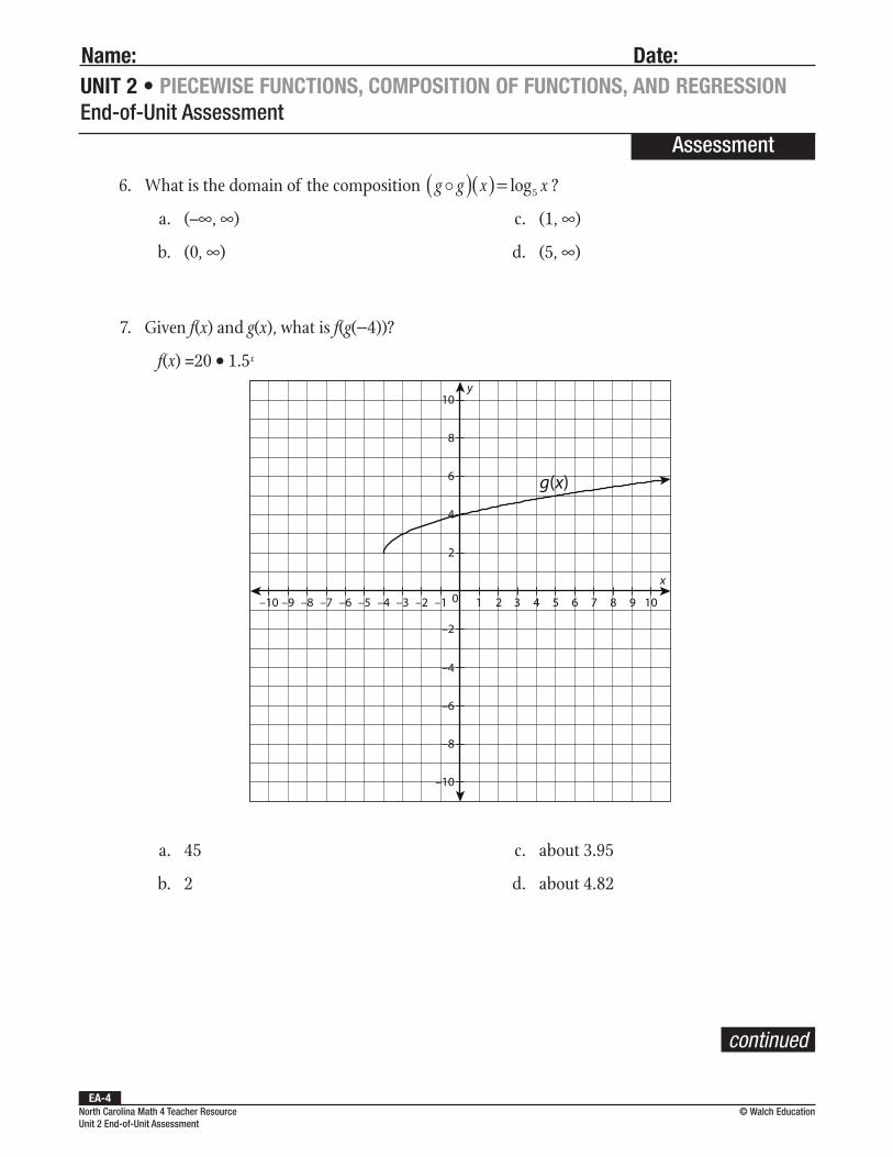
North Carolina Math 4 Teacher Resource Unit 2 End-of-Unit Assessment
© Walch EducationEA-4
UNIT 2 • PIECEWISE FUNCTIONS, COMPOSITION OF FUNCTIONS, AND REGRESSIONEnd-of-Unit Assessment
Assessment
Name: Date:
6. What is the domain of the composition g g x xlog5( )( )= ?
a. (–∞, ∞)
b. (0, ∞)
c. (1, ∞)
d. (5, ∞)
7. Given f(x) and g(x), what is f(g(−4))?
f(x) =20 • 1.5x
2 4 6 8 10
10
1 3 5 7 9
–2
–4
–6
–8
8
6
4
2
0
y
x
–10
–1–2–3–4–5–6–7–8–9–10
g(x)
a. 45
b. 2
c. about 3.95
d. about 4.82
continued
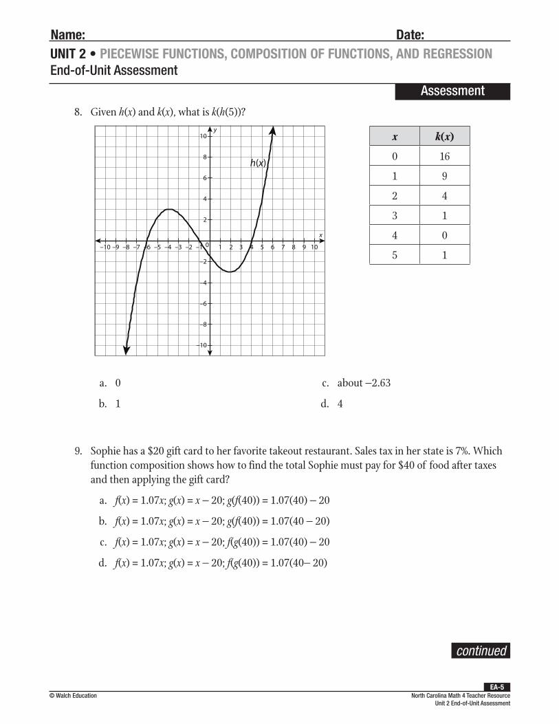
North Carolina Math 4 Teacher Resource Unit 2 End-of-Unit Assessment
© Walch EducationEA-5
UNIT 2 • PIECEWISE FUNCTIONS, COMPOSITION OF FUNCTIONS, AND REGRESSIONEnd-of-Unit Assessment
Assessment
Name: Date:
8. Given h(x) and k(x), what is k(h(5))?
2 4 6 8 10
10
1 3 5 7 9
–2
–4
–6
–8
8
6
4
2
0
y
x
–10
–1–2–3–4–5–6–7–8–9–10
h(x)
x k(x)
0 16
1 9
2 4
3 1
4 0
5 1
a. 0
b. 1
c. about −2.63
d. 4
9. Sophie has a $20 gift card to her favorite takeout restaurant. Sales tax in her state is 7%. Which function composition shows how to find the total Sophie must pay for $40 of food after taxes and then applying the gift card?
a. f(x) = 1.07x; g(x) = x − 20; g(f(40)) = 1.07(40) − 20
b. f(x) = 1.07x; g(x) = x − 20; g(f(40)) = 1.07(40 − 20)
c. f(x) = 1.07x; g(x) = x − 20; f(g(40)) = 1.07(40) − 20
d. f(x) = 1.07x; g(x) = x − 20; f(g(40)) = 1.07(40− 20)
continued
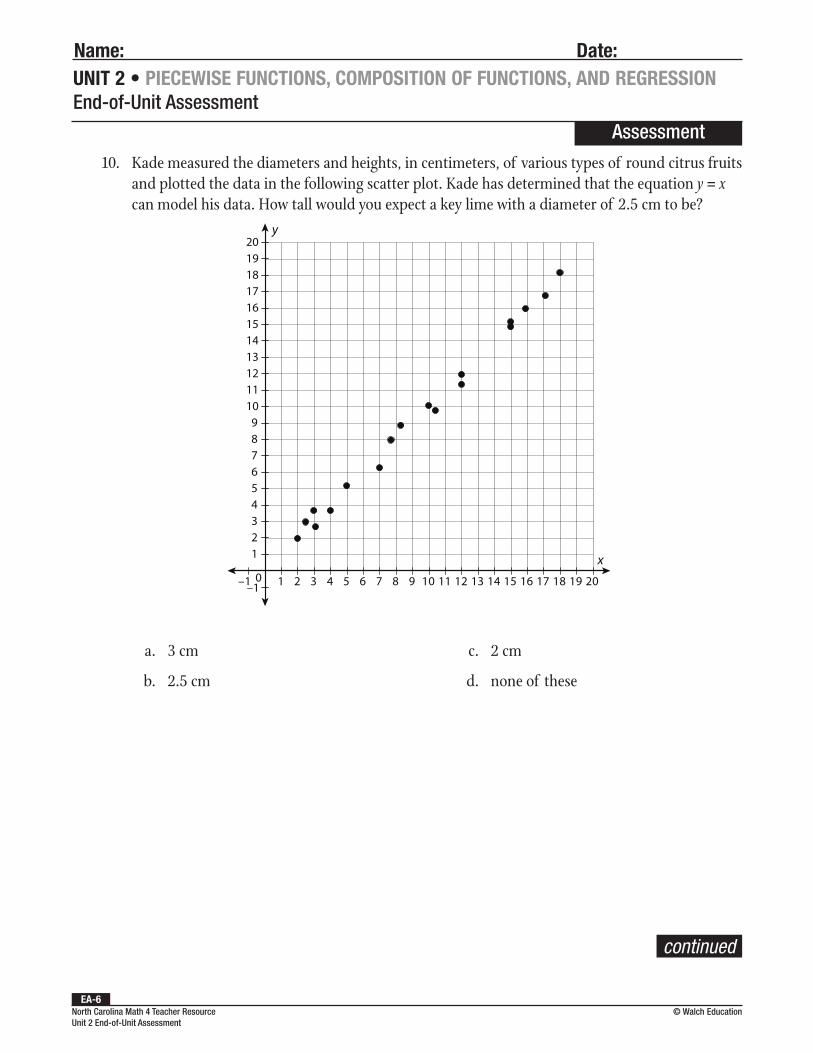
North Carolina Math 4 Teacher Resource Unit 2 End-of-Unit Assessment
© Walch EducationEA-6
UNIT 2 • PIECEWISE FUNCTIONS, COMPOSITION OF FUNCTIONS, AND REGRESSIONEnd-of-Unit Assessment
Assessment
Name: Date:
10. Kade measured the diameters and heights, in centimeters, of various types of round citrus fruits and plotted the data in the following scatter plot. Kade has determined that the equation y = x can model his data. How tall would you expect a key lime with a diameter of 2.5 cm to be?
2 4 6 8 10
10
8
6
4
2
7
5
3
1
0
9
1 3 5 7 9
y
12 14 16 18 2011 13 15 17 19
20
18
16
14
12
17
15
13
11
19
x
–1–1
a. 3 cm
b. 2.5 cm
c. 2 cm
d. none of these
continued

North Carolina Math 4 Teacher Resource Unit 2 End-of-Unit Assessment
© Walch EducationEA-7
UNIT 2 • PIECEWISE FUNCTIONS, COMPOSITION OF FUNCTIONS, AND REGRESSIONEnd-of-Unit Assessment
Assessment
Name: Date:
11. Which regression model is the best fit for the data in the following scatter plot?
2 4 6 8 10
10
8
6
4
2
7
5
3
1
0
9
1 3 5 7 9
y
12 14 16 18 2011 13 15 17 19
20
18
16
14
12
17
15
13
11
19
x
–1–1
a. y = 0.98x − 3.15
b. y = 0.1x2 − 0.73x + 2.05
c. y = 0.6 • 1.23x
d. None of these are a good fit.
continued
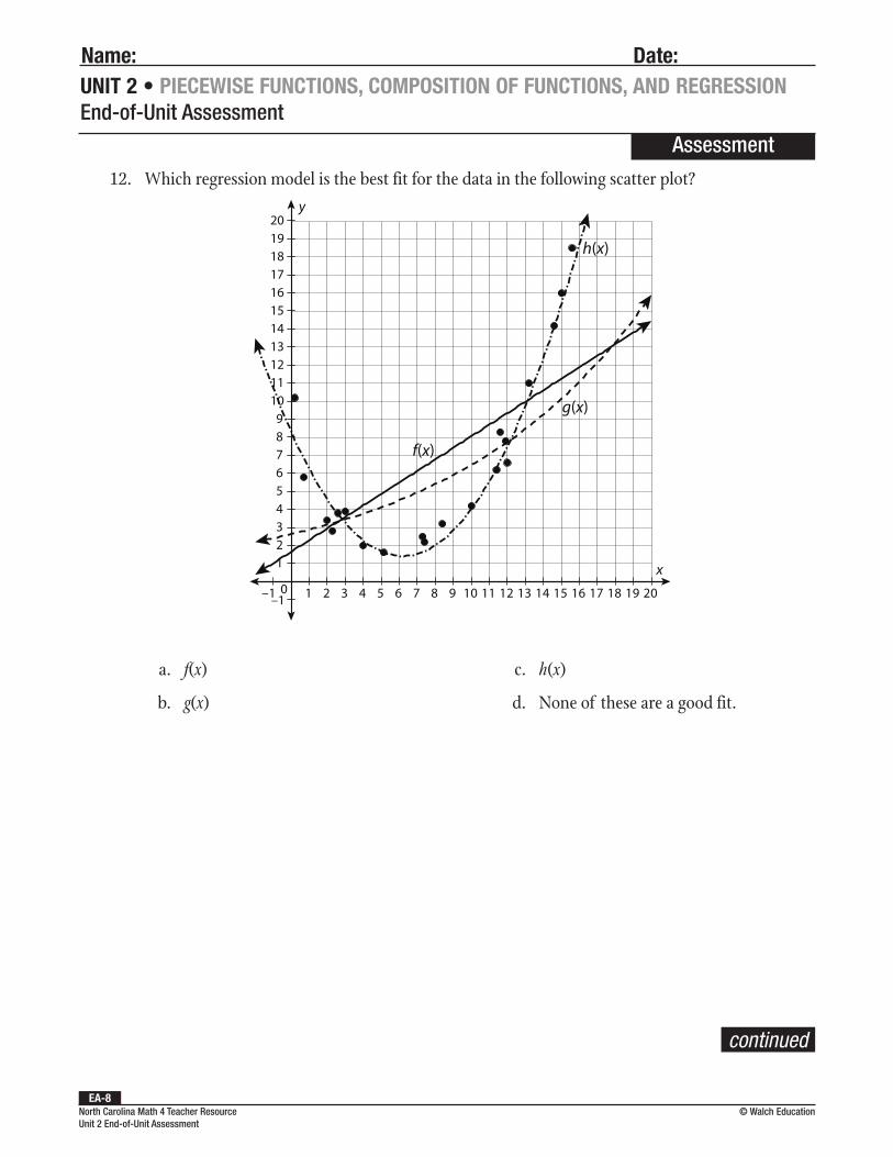
North Carolina Math 4 Teacher Resource Unit 2 End-of-Unit Assessment
© Walch EducationEA-8
UNIT 2 • PIECEWISE FUNCTIONS, COMPOSITION OF FUNCTIONS, AND REGRESSIONEnd-of-Unit Assessment
Assessment
Name: Date:
12. Which regression model is the best fit for the data in the following scatter plot?
f(x)
2 4 6 8 10
10
8
6
4
2
7
5
3
1
0
9
1 3 5 7 9
y
12 14 16 18 2011 13 15 17 19
20
18
16
14
12
17
15
13
11
19
x
–1–1
h(x)
g(x)
a. f(x)
b. g(x)
c. h(x)
d. None of these are a good fit.
continued

North Carolina Math 4 Teacher Resource Unit 2 End-of-Unit Assessment
© Walch EducationEA-9
UNIT 2 • PIECEWISE FUNCTIONS, COMPOSITION OF FUNCTIONS, AND REGRESSIONEnd-of-Unit Assessment
Assessment
Name: Date:
13. Gila fit a linear function to her data and plotted the residuals. The residual plot is shown in the following graph. Which of the following statements best describes the residual graph?
2 4 6 8 10
10
8
6
4
2
7
5
3
10
9
1 3 5 7 9 12 14 16 18 2011 13 15 17 19
x
–1
y
–2
–4
–6
–8
–10
–5
–7
–9
–3
a. A linear function is a good fit for the data.
b. A linear function is not a good fit for the data. She should use a quadratic function.
c. A linear function is not a good fit for the data. She should use an exponential function.
d. A linear function is not a good fit for the data. She should not use a linear function, but it cannot be determined from the given information what model is best to use instead.
continued

North Carolina Math 4 Teacher Resource Unit 2 End-of-Unit Assessment
© Walch EducationEA-10
UNIT 2 • PIECEWISE FUNCTIONS, COMPOSITION OF FUNCTIONS, AND REGRESSIONEnd-of-Unit Assessment
Assessment
Name: Date:
14. A linear and a quadratic function were fitted to a data set. Their residual plots are shown in the following graphs. Which function is the better fit?
Linear
2 4 6 8 10
10
8
6
4
2
7
5
3
10
9
1 3 5 7 9 12 14 16 18 2011 13 15 17 19
x
–1
y
–2
–4
–6
–8
–10
–5
–7
–9
–3
Quadratic
2 4 6 8 10
10
8
6
4
2
7
5
3
10
9
1 3 5 7 9 12 14 16 18 2011 13 15 17 19
x
–1
y
–2
–4
–6
–8
–10
–5
–7
–9
–3
a. linear
b. quadratic
c. Both functions are a good fit.
d. Neither function is a good fit.
continued

North Carolina Math 4 Teacher Resource Unit 2 End-of-Unit Assessment
© Walch EducationEA-11
UNIT 2 • PIECEWISE FUNCTIONS, COMPOSITION OF FUNCTIONS, AND REGRESSIONEnd-of-Unit Assessment
Assessment
Name: Date:
15. A quadratic and an exponential function were fitted to a data set. Their residual plots are shown in the following graphs. Which function is the better fit?
Quadratic
2 4 6 8 10
10
8
6
4
2
7
5
3
10
9
1 3 5 7 9 12 14 16 18 2011 13 15 17 19
x
–1
y
–2
–4
–6
–8
–10
–5
–7
–9
–3
Exponential
2 4 6 8 10
10
8
6
4
2
7
5
3
10
9
1 3 5 7 9 12 14 16 18 2011 13 15 17 19
x
–1
y
–2
–4
–6
–8
–10
–5
–7
–9
–3
a. quadratic
b. exponential
c. Both functions are a good fit.
d. Neither function is a good fit.

North Carolina Math 4 Teacher Resource Unit 2 End-of-Unit Assessment
© Walch EducationEA-12
UNIT 2 • PIECEWISE FUNCTIONS, COMPOSITION OF FUNCTIONS, AND REGRESSIONEnd-of-Unit Assessment
Instruction
Unit 2 End-of-Unit Assessment Answer Key
Answer Standard(s)
1. d NC.M4.AF.4.1
2. a NC.M4.AF.4.1, NC.M4.AF.4.2
3. a NC.M4.AF.4.2
4. d NC.M4.AF.1.1
5. c NC.M4.AF.1.1
6. c NC.M4.AF.1.1
7. a NC.M4.AF.1.2
8. a NC.M4.AF.1.2
9. a NC.M4.AF.1.2
10. b NC.M4.AF.5.1
11. c NC.M4.AF.5.1
12. c NC.M4.AF.5.1
13. d NC.M4.AF.5.2
14. a NC.M4.AF.5.2
15. b NC.M4.AF.5.2