NNT - Software Manual
210
Rev. 2.5 – March, 1 st 2011 Page 1 of 210 NNT MANUAL Software Version 3.10 Rev. 2.5 March, 1 st 2011 Cod. 97050192
-
Upload
carlrossus -
Category
Documents
-
view
246 -
download
10
Transcript of NNT - Software Manual
Rev. 2.5 – March, 1st 2011 Page 1 of 210
NNT
MANUALSoftware Version 3.10
Rev. 2.5March, 1st 2011
Cod. 97050192

Rev. 2.5 – March, 1st 2011 Page 2 of 210
NOTES:This document is provided for the own use of the operator of the equipment.
QR s.r.l. reserves the right to change the contents of this manual without notice.
This document may not, in whole or in part, be modified, copied, reproduced, distributed, translated, storedon magnetic or optical media and published, over networks, electronic bulletin boards, web sites or other on-line services, without the express written permission of QR s.r.l.
The original version of this manual has been written in english language.
NNT is a registered trademark of QR s.r.l.All other products and brand names are registered trademarks or trademarks of their respective companies.
NNT is manufactured and distributed by:
QR srlVia Silvestrini, 2037135 VeronaItalyPhone: ++39 045 8202727Fax ++39 045 8203040e-mail: info @qrverona.itwww.qrverona.it
All rights reserved.
Rev. 2.5 – March, 1st 2011 Page 3 of 210
TABLE OF CONTENTS
1 ABOUT THIS MANUAL................................. ....................................................................................... 7
1.1 CONTENTS........................................................................................................................................... 71.2 DEFINITIONS ........................................................................................................................................ 71.3 STRUCTURE ......................................................................................................................................... 71.4 STILISTIC CONVENTIONS ........................................................................................................................ 8
2 GETTING STARTED............................................................................................................................ 9
2.1 SOFTWARE INSTALLATION...................................................................................................................... 92.2 SOFTWARE CONFIGURATION .................................................................................................................. 92.3 WORKSTATION ....................................................................................................................................10
2.3.1 Newtwork switches......................................................................................................................112.3.2 Validated graphic cards...............................................................................................................12
2.4 MAIN WINDOW .....................................................................................................................................132.5 DEVICES DIFFERENCES.........................................................................................................................14
3 PRESCAN OPERATIONS................................ ...................................................................................15
3.1 PERFORMING THE X-RAY SOURCE CONDITIONING ...................................................................................153.2 RUNNING A DAILY CHECK ......................................................................................................................163.3 COLLIMATOR CHECK.............................................................................................................................173.4 BLANK ACQUISITION.............................................................................................................................18
4 SCANNING .........................................................................................................................................19
4.1 SCANNING A PATIENT ...........................................................................................................................194.1.1 Selecting the FOV for scanning ...................................................................................................194.1.2 Entering a patient’s data..............................................................................................................204.1.3 Positioning the patient and running the scan................................................................................22
4.2 SCANNING A DENTURE..........................................................................................................................264.2.1 Preliminary operations.................................................................................................................264.2.2 Positioning the denture and starting a new scan..........................................................................27
4.3 SCANNING A PATIENT OR A DENTURE IN A THIRD-PARTY SOFTWARE ENVIROMENT ........................................304.4 REMOTE PATIENT POSITION ADJUSTMENT ...............................................................................................30
5 RUNNING A PRIMARY RECONSTRUCTION .................. ...................................................................32
5.1 INTRODUCTION ....................................................................................................................................325.2 OPENING RAWDATA ............................................................................................................................325.3 RAWDATA WINDOW .............................................................................................................................345.4 CHECKING THE SCAN............................................................................................................................365.5 MODIFYING THE PRIMARY RECONSTRUCTION PARAMETERS......................................................................37
5.5.1 Procedure for devices with automatic reconstruction ...................................................................375.5.2 Procedure for devices with manual reconstruction or with Advanced mode enabled.....................375.5.3 Procedure for devices with Primary & Study reconstruction enabled ............................................385.5.4 Reconstruction parameters window.............................................................................................38
5.6 STARTING A PRIMARY RECONSTRUCTION ...............................................................................................405.7 STARTING PRIMARY & STUDY RECONSTRUCTIONS ..................................................................................435.8 NIGHT RECONSTRUCTION.....................................................................................................................45
5.8.1 Storing multiple Primary Reconstructions ....................................................................................455.8.2 Running multiple primary reconstruction......................................................................................45
5.9 MANAGEMENT OF NON RECONSTRUCTED SCAN .......................................................................................46
6 VOLUMETRIC DATA ................................... .......................................................................................47
6.1 INTRODUCTION ....................................................................................................................................476.2 OPENING A VOLUMETRIC DATA .............................................................................................................476.3 VOLUMETRIC VIEW ...............................................................................................................................496.4 MPR VIEW..........................................................................................................................................50
6.4.1 Modifying the zoom .....................................................................................................................526.5 MODIFYING THE STUDY RECONSTRUCTION PARAMETERS .........................................................................536.6 CREATING A NEW STUDY.......................................................................................................................546.7 MULTIPLE STUDY RECONSTRUCTIONS ....................................................................................................56
Rev. 2.5 – March, 1st 2011 Page 4 of 210
6.8 EXPORTING THE AXIAL IMAGES IN DICOM FORMAT..................................................................................57
7 WORKING WITH A STUDY.............................. ...................................................................................58
7.1 INTRODUCTION ....................................................................................................................................587.2 OPENING A STUDY ...............................................................................................................................587.3 STUDY WINDOW...................................................................................................................................597.4 AXIAL IMAGES .....................................................................................................................................61
7.4.1 What is an axial image? ..............................................................................................................617.4.2 Axial images overview.................................................................................................................617.4.3 Moving among axial images. .......................................................................................................62
7.5 CREATING NEW IMAGES ........................................................................................................................637.5.1 Single Cross Sections .................................................................................................................637.5.2 Sequence of Cross Sections .......................................................................................................657.5.3 Panoramic Sections ....................................................................................................................687.5.4 Multiplanar images ......................................................................................................................707.5.5 3D MIP, Ray Cast and Volume images........................................................................................737.5.6 Dynamic 3D images ....................................................................................................................84
7.6 DELETING EXISTING IMAGES. .................................................................................................................887.6.1 Deleting single cross sections from a sequence of cross sections................................................88
7.7 FUNCTIONS TO EXTRACT AND CONVERT IMAGES. .....................................................................................897.7.1 Extracting single cross sections from a sequence of cross sections .............................................897.7.2 Extracting panoramic sections from a multiplanar image..............................................................927.7.3 Extracting sequence of cross sections from a multiplanar image..................................................937.7.4 Extracting Coronal and Sagittal sections from the MPR view .......................................................947.7.5 Converting a Panoramic image into a Sequence of Cross Sections. ............................................957.7.6 Converting a Sequence of Cross Sections into a Panoramic image. ............................................96
7.8 MODIFYING AN EXISTING IMAGE. ............................................................................................................977.8.1 Standard drag .............................................................................................................................977.8.2 Real time drag.............................................................................................................................997.8.3 Modifying the axial stack ...........................................................................................................100
7.9 MOVING AMONG DIFFERENT IMAGES.....................................................................................................1027.10 MODIFYING IMAGE APPEARANCE. .......................................................................................................102
7.10.1 Visualization window ...............................................................................................................1027.10.2 Modifying the zoom .................................................................................................................104
7.11 MANAGING IMAGES. .........................................................................................................................1057.11.1 Saving the study configuration.................................................................................................105
7.12 HIDING THE IMAGES OVERLAYS..........................................................................................................1067.13 SAVING IMAGES IN DIFFERENT FILE FORMATS ......................................................................................106
7.13.1 Screen shot command ............................................................................................................1077.14 EXPORTING/IMPORTING THE AXIAL IMAGES IN DICOM FORMAT ............................................................107
7.14.1 Exporting the axial images in DICOM format ...........................................................................1087.14.2 Importing the axial images in DICOM format............................................................................1087.14.3 DICOM Settings ......................................................................................................................1097.14.4 Integration between NNT and third party softwares (partnering software).................................109
7.15 WORKING WITH TOOLBARS................................................................................................................1107.15.1 Images creation toolbar ...........................................................................................................1107.15.2 Working with angles ................................................................................................................1107.15.3 Working with lines and arrows .................................................................................................1137.15.4 Working with distances............................................................................................................1197.15.5 Working with 3D distances ......................................................................................................1237.15.6 Working with markers..............................................................................................................1267.15.7 Working with profiles ...............................................................................................................1277.15.8 Working with text.....................................................................................................................1297.15.9 Tools Toolbar ..........................................................................................................................135
7.16 ENABLE/DISABLE THE DELETE CONFIRMATION MESSAGES.....................................................................135
8 TEMPLATES......................................... ............................................................................................137
8.1 INTRODUCTION ..................................................................................................................................1378.2 CREATING A NEW TEMPLATE ...............................................................................................................1378.3 MODIFYING AN EXISTING TEMPLATE .....................................................................................................1408.4 DELETING TEMPLATES ........................................................................................................................141

Rev. 2.5 – March, 1st 2011 Page 5 of 210
8.5 CONVERTING A TEMPLATE ..................................................................................................................1428.6 COPYING A TEMPLATE ........................................................................................................................143
9 WORKING WITH REPORTS .............................................................................................................145
9.1 CREATING A NEW REPORT ..................................................................................................................1459.1.1 Open a template .......................................................................................................................1459.1.2 Add images to the report ...........................................................................................................1479.1.3 Automated images insertion ......................................................................................................1499.1.4 Delete images from a report ......................................................................................................1509.1.5 Insert notes in the report ...........................................................................................................1509.1.6 Remove notes from the report ...................................................................................................1529.1.7 Report notes database ..............................................................................................................1529.1.8 Adding new pages to a report....................................................................................................1539.1.9 Removing pages from a report ..................................................................................................154
9.2 ADVANCED REPORT FUNCTIONS ..........................................................................................................1559.2.1 Modifying the template of a report page.....................................................................................1559.2.2 Modifying the appearance of the report images .........................................................................1559.2.3 Use of the “Draw Only On Reference Image” menu item. ..........................................................1569.2.4 Use of the “Highlight crosses on panoramics” menu item...........................................................1579.2.5 Performing measures of distances or angles .............................................................................1589.2.6 Including exam/pazient data in the report ..................................................................................159
9.3 PRINTING A REPORT ...........................................................................................................................1599.4 SAVING A REPORT..............................................................................................................................1599.5 SAVING A REPORT IN PDF FORMAT .....................................................................................................1609.6 OPENING A REPORT...........................................................................................................................160
9.6.1 Modifying the patient’s data of a report ......................................................................................161
10 OTHER FUNCTIONS.....................................................................................................................162
10.1 EDITING THE HEADER OF THE REPORT ................................................................................................16210.2 ENABLING THE “ADVANCED MODE” OPTION .........................................................................................16410.3 MODIFYING THE NNT THEMES...........................................................................................................16410.4 MODIFY THE APPEARANCE OF THE GRAPHICS TOOLS............................................................................165
10.4.1 Using the GDI+ options ...........................................................................................................16810.4.2 Changing the report colors ......................................................................................................16810.4.3 Select the data to be included in the report ..............................................................................16910.4.4 Changing the Overlay Color Conversion (B/W printers only) ....................................................17010.4.5 Changing the Printer color usage and color conversion ...........................................................17010.4.6 Print Optimize..........................................................................................................................17110.4.7 Apply a ruler on the images.....................................................................................................171
10.5 REPORT PRINT ENHANCEMENT ..........................................................................................................17210.6 3M PRINTERS & DICOM ..................................................................................................................17310.7 SYSTEM FILES BACKUP .....................................................................................................................17510.8 USE OF THE VDDS PROTOCOL .........................................................................................................175
11 MANAGING DOCUMENTS............................... .............................................................................177
11.1 IMPORTING DOCUMENTS ...................................................................................................................17711.1.1 Importing by document............................................................................................................17711.1.2 Importing by patient.................................................................................................................178
11.2 IMPORTING OLD NEWTOM SCAN.........................................................................................................17911.3 EXPORTING DOCUMENTS ..................................................................................................................179
11.3.1 Export by patient .....................................................................................................................17911.3.2 Export by document ................................................................................................................181
11.4 DELETE DOCUMENTS .......................................................................................................................18311.5 CREATE CDS AND DVDS..................................................................................................................183
11.5.1 Create a disc by Document .....................................................................................................18411.5.2 Create a disc by Patient ..........................................................................................................18411.5.3 Create a Free Viewer ..............................................................................................................18511.5.4 NNTBurner..............................................................................................................................186
12 QUALITY ASSURANCE ................................ ................................................................................189
12.1 SELECTING THE FOV FOR THE SCAN..................................................................................................189
Rev. 2.5 – March, 1st 2011 Page 6 of 210
12.2 RUNNING THE QA SCAN ...................................................................................................................18912.3 TROUBLESHOOTING .........................................................................................................................19612.4 SAMPLES OF IMAGES ........................................................................................................................19612.5 COPY OF QA IMAGES .......................................................................................................................19712.6 STORAGE OF QA DATA.....................................................................................................................197
13 TROUBLESHOOTING.................................. .................................................................................198
13.1 ERRORS GUIDE ...............................................................................................................................19813.2 LOG ERROR ....................................................................................................................................19813.3 REMOTE SUPPORT ...........................................................................................................................199
14 IEC61223 STANDARD: ACCEPTANCE TEST ............... ...............................................................200
14.1 POSITIONING OF THE PATIENT SUPPORT [PARAGRAPH 5.1]....................................................................20014.2 PATIENT POSITIONING ACCURACY [PARAGRAPH 5.2] ............................................................................200
14.2.1 Axial patient positioning accuracy [paragraph 5.2.1] ................................................................20014.2.2 Sagittal and coronal patient positioning light [paragraph 5.2.2].................................................200
14.3 TOMOGRAPHIC SECTION THICKNESS [PARAGRAPH 5.3].........................................................................20114.3.1 Tomographic section thickness for axial scanning [paragraph 5.3.1] ........................................20114.3.2 Tomographic section thickness for helical scanning [paragraph 5.3.2] .....................................204
14.4 DOSE [PARAGRAPH 5.4] ...................................................................................................................20414.5 NOISE, MEAN CT NUMBER AND UNIFORMITY [PARAGRAPH 5.5]..............................................................20414.6 SPATIAL RESOLUTION [PARAGRAPH 5.6] .............................................................................................207
15 APPENDIX A ....................................... ..........................................................................................210
15.1 GETTING OUT THE SOFTWARE ...........................................................................................................21015.2 CHECKING THE CONNECTION BETWEEN COMPUTER AND SCANNER.........................................................21015.3 RUNNING THE X-RAY SOURCE FORMING PROCESS...............................................................................210
Quality assurance
Rev. 2.5 – March, 1st 2011 Page 7 of 210
1 About this Manual
1.1 ContentsThis manual has been conceived as a mean of reference to provide information and instructions on the useof the NNT software.The user shall fully read and understand this manual before using the equipment. It is highly recommendedto keep this manual along with further documentation and to use it as an handbook in order to instruct newstaff in using the equipment.
1.2 Definitions
Definition Meaning
MAIN WORKSTATION Computer connected the CT scan.
SECONDARY WORKSTATIONAny computer running NNT software for the sole data processing/view.
Thus, all the MAIN WORKSTATIONS are excluded from thiscathegory.
MACHINE USER MANUAL Manual dedicated to the equipment running the NNT software.
FOV Acronym of Field Of View.
MULTI FOV DEVICE Equipment which allows to switch to a different FOV.
1.3 StructureThis manual includes the following sections:
• Chapter 1 (“About this Manual ”): provides general information about the structure and the stylisticconventions of the manual.
• Chapter 2 (“Getting started ”): contains a general description of the machine and its maincomponents.
• Chapter 3 (“Errore. L'origine riferimento non è stata trovata.”): illustrates the steps to run the dailycheck procedure.
• Chapter 4 (“Scanning ”): contains the description of the procedure to scan a patient.• Chapter 5 (“Running a Primary Reconstruction ”): describes the Primary Reconstruction process
and the steps to run it.• Chapter 6 (“Volumetric Data ”): introduces the volumetric data views and includes the procedure to
create a study.• Chapter 7 (“Working with a Study ”): contains the description of all the tools and utilities to perform
a secondary reconstruction and a complete analysis of the study.• Chapter 8 (“Templates ”): introduces the templates and illustrates how to create, modify and delete
templates.• Chapter 0 (“Working with reports ”): illustrates the steps to create a report and the related utilities.• Chapter 10 (“Other functions ”): contains the description of other functionality included in the
software.• Chapter 11 (“Managing documents ”): describes how to manage the different type of documents
(raw data, volumetric data, study and report).• Chapter 12 (“Quality assurance ”): illustrates the steps to run the Quality Assurance process.• Chapter 13 (“

About this manual
Rev. 2.5 – March, 1st 2011 Page 8 of 210
• Troubleshooting”): illustrates how to spot and solve problems.• Chapter 14 (“IEC61223 Standard: Acceptance Test ”): illustrates the software utilities to perform
equipment Acceptance Test according to IEC61223 Standard.
• APPENDIX A: it illustrates some utilities not tackled in other chapters.
1.4 Stilistic conventionsThe following table illustrates the stylistic conventions adopted by this manual:
Text format Example Meaning
Bold Italic File →→→→ Open… Menu or toolbar item
Italic Patient File Window Title
Bold Underlined Apply Button Command
<text> <Demonstration template> Typed text
CAPITAL LETTER ENTER keyboard command
Important safety information and notes are highlighted in the manual as follows:
WARNING:Warns you of the presence of a potential hazard, which may cause injury or fatality.
CAUTION:Cautions you of the presence of a potential hazard, which may cause damage to theequipment.
NOTE:Draws your attention to important but non-hazardous information.
Getting started
Rev. 2.5 – March, 1st 2011 Page 9 of 210
2 Getting started
2.1 Software installationIn order to properly install and uninstall NNT software, the user shall refer to the documentation included intothe setup CD.
2.2 Software configurationThis paragraph provides with a description of the various available NNT software suites which can beconfigured by using a specific USB dongle key (not in case of Basic configuration).
Hereafter a brief description of each NNT software suite is provided:
SCAN TM: NNT Scan TM suite is used to control the equipment. It allows to perform scanning and primaryreconstruction.The acquired data can be saved on a local computer or sent to the network which the computer is connectedto (thus, processed by other workstation provided with a different NNT software configuration/suite).
EXPERT: NNT Expert suite allows to perform all the NNT tasks. In particular, if the computer which the NNTExpert suite is installed on is a PRIMARY WORKSTATION (see paragraph “1.2 Definitions ”), the user willbe able to perform scanning along with all the other tasks (primary, volumetric, secondary and 3D imagingreconstructions, and report creation and printing). Otherwise, if the computer is a SECONDARYWORKSTATION (see paragraph “1.2 Definitions ”), it will be possible to perform all the above mentionedtasks but scanning.
PROFESSIONAL: NNT Professional suite allows to create new studies, to perform secondary reconstructionand to create and print reports, beginning from volumetric data (created by primary reconstruction).
BASIC: NNT Basic suite allows to view, print, and save into a personale archive, previously created reports.The user will be also able to add distance and angle measurements and to modify images brightness andcontrast.
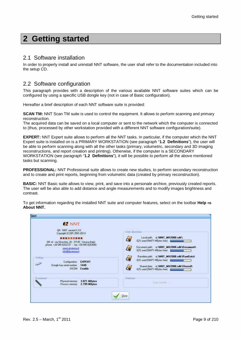
To get information regarding the installed NNT suite and computer features, select on the toolbar Help ⇒⇒⇒⇒About NNT.
Getting started
Rev. 2.5 – March, 1st 2011 Page 10 of 210
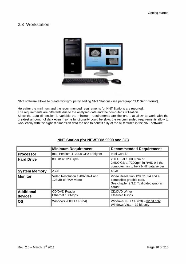
2.3 Workstation
NNT software allows to create workgroups by adding NNT Stations (see paragraph “1.2 Definitions ”).
Hereafter the minimum and the recommended requirements for NNT Stations are reported.The requirements are differents due to the analysed data and the computer’s utilization.Since the data dimension is variable the minimum requirements are the one that allow to work with thegreatest amounth of data even if some functionality could be slow; the recommended requirements allow towork easily with the highest dimension data too and to benefit fully of the all features in the NNT software.
NNT Station (for NEWTOM 9000 and 3G)
Minimum Requirement Recommended RequirementProcessor Intel Pentium 4 ≥ 2.8 GHz or higher Intel Core i7
Hard Drive 80 GB at 7200 rpm 250 GB at 10000 rpm or2x500 GB at 7200rpm in RAID 0 if thecomputer has to be a NNT data server
System Memory 2 GB 4 GB
Monitor Video Resolution 1280x1024 and128MB of RAM video
Video Resolution 1280x1024 and acompatible graphic card.See chapter 2.3.2 “Validated graphiccards”
Additionaldevices
CD/DVD ReaderEthernet 100Mbps
CD/DVD WriterEthernet 1Gbps
OS Windows 2000 + SP (≥4) Windows XP + SP (≥3) – 32 bit onlyWindows Vista – 32 bit only
Getting started
Rev. 2.5 – March, 1st 2011 Page 11 of 210
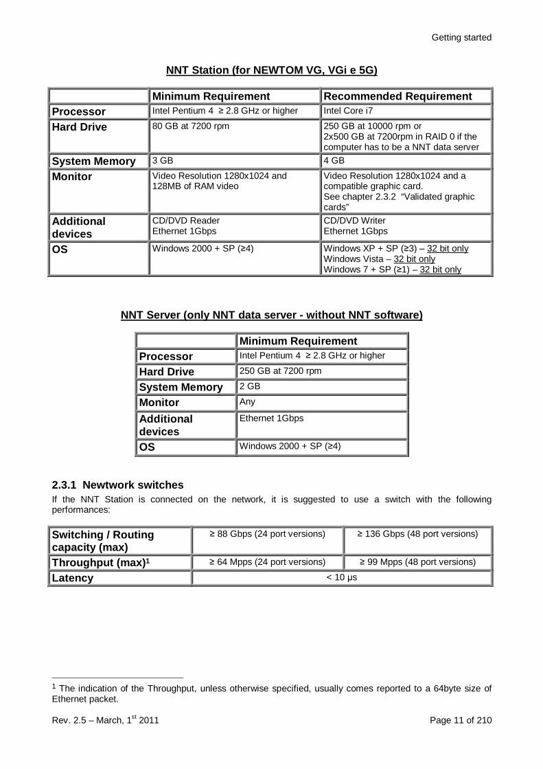
NNT Station (for NEWTOM VG, VGi e 5G)
Minimum Requirement Recommended RequirementProcessor Intel Pentium 4 ≥ 2.8 GHz or higher Intel Core i7
Hard Drive 80 GB at 7200 rpm 250 GB at 10000 rpm or2x500 GB at 7200rpm in RAID 0 if thecomputer has to be a NNT data server
System Memory 3 GB 4 GB
Monitor Video Resolution 1280x1024 and128MB of RAM video
Video Resolution 1280x1024 and acompatible graphic card.See chapter 2.3.2 “Validated graphiccards”
Additionaldevices
CD/DVD ReaderEthernet 1Gbps
CD/DVD WriterEthernet 1Gbps
OS Windows 2000 + SP (≥4) Windows XP + SP (≥3) – 32 bit onlyWindows Vista – 32 bit onlyWindows 7 + SP (≥1) – 32 bit only
NNT Server (only NNT data server - without NNT soft ware)
Minimum RequirementProcessor Intel Pentium 4 ≥ 2.8 GHz or higher
Hard Drive 250 GB at 7200 rpm
System Memory 2 GB
Monitor Any
Additionaldevices
Ethernet 1Gbps
OS Windows 2000 + SP (≥4)
2.3.1 Newtwork switchesIf the NNT Station is connected on the network, it is suggested to use a switch with the followingperformances:
Switching / Routingcapacity (max)
≥ 88 Gbps (24 port versions) ≥ 136 Gbps (48 port versions)
Throughput (max) 1 ≥ 64 Mpps (24 port versions) ≥ 99 Mpps (48 port versions)
Latency < 10 µs
1 The indication of the Throughput, unless otherwise specified, usually comes reported to a 64byte size ofEthernet packet.

Getting started
Rev. 2.5 – March, 1st 2011 Page 12 of 210
2.3.2 Validated graphic cardsThese graphic cards have been tested and validated in QR for using with NNT software:ATI Radeon HD 4850 / 4870 / 4890 / 5770 / 5850 / 5870 / 6850 / 6870 with 1GB or greater.Sapphire Radeon HD 6750 / 6770 – VaporX – 1GB (or greater) – RAM GDDR5.Sapphire Radeon HD 6950 – VaporX if available – 1GB (or greater) – RAM GDDR5.Sapphire Radeon HD 6970 – VaporX if available – 2GB (or greater) – RAM GDDR5.
Getting started
Rev. 2.5 – March, 1st 2011 Page 13 of 210
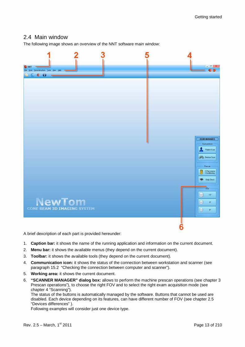
2.4 Main windowThe following image shows an overview of the NNT software main window:
A brief dexcription of each part is provided hereunder:
1. Caption bar: it shows the name of the running application and information on the current document.
2. Menu bar: it shows the available menus (they depend on the current document).
3. Toolbar: it shows the available tools (they depend on the current document).
4. Communication icon: it shows the status of the connection between workstation and scanner (seeparagraph 15.2 “Checking the connection between computer and scanner”).
5. Working area: it shows the current document.
6. “SCANNER MANAGER” dialog box: allows to perform the machine prescan operations (see chapter 3Prescan operations”), to choose the right FOV and to select the right exam acquisition mode (seechapter 4 “Scanning”).The status of the buttons is automatically managed by the software. Buttons that cannot be used aredisabled. Each device depending on its features, can have different number of FOV (see chapter 2.5“Devices differences” ).Following examples will consider just one device type.

Getting started
Rev. 2.5 – March, 1st 2011 Page 14 of 210
2.5 Devices differencesThis chapter shows the software differences based on used equipment type.The explanation of each single option will be covered in the related chapter.
Available Field Of Views (FOV):
NewTom 3G 12” NewTom VG NewTom VG 3 FOVNewTom VGi 3 FOV NewTom VGi 7 FOV NewTom 5G
Management of the scan data and primary reconstruction options:
Manual Automatic Advancedmode
Primary &study
Voxel options Scan optionchoice
NewTom DVT9000 9000NewTom 3G X X 3GNewTom VG X StandardNewTom VGi 3 FOV X X AdvancedNewTom 5G X X Advanced XNewTom VGi 7 FOV X X Advanced
Daily Check
Rev. 2.5 – March, 1st 2011 Page 15 of 210
3 Prescan operations
In this chapter are described all the mandatory operations to be performed before the patient acquisitions.Some of these operations must be performed every day depending on the scanner model.It will not be possible to perform a patient’s scan before the above mentioned operations are successfullycompleted.This chapter only regards MAIN WORKSTATIONS (see paragraph “1.2 Definitions”).Refer to the MACHINE USER MANUAL to know when and how to do do these prescan operations.
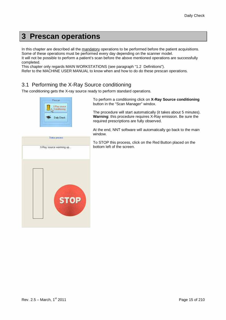
3.1 Performing the X-Ray Source conditioningThe conditioning gets the X-ray source ready to perform standard operations.
To perform a conditioning click on X-Ray Source conditioningbutton in the “Scan Manager” windox.
The procedure will start automatically (it takes about 5 minutes).Warning : this procedure requires X-Ray emission. Be sure therequired prescriptions are fully observed.
At the end, NNT software will automatically go back to the mainwindow.
To STOP this process, click on the Red Button placed on thebottom left of the screen.

Daily Check
Rev. 2.5 – March, 1st 2011 Page 16 of 210
3.2 Running a daily checkThrough the daily check the system verifies whether all the components are operating properly.
To run a daily check click on Daily Check button on the “ScanManager” window.
Note: Daily Check will start automatically after the X-Ray sourceConditioning Procedure described before.
Make sure the gantry is empty (see MACHINE USER MANUAL,see paragraph “1.2 Definitions ”).
The “Daily check” window will open.
Click on “Start ” to begin the process.
The system will perform each test and display the resulting statusin real time.
When the last test is completed click on “Close ”.
Now it is possible to scan a patient.
During the daily check two types of error can occur. The critical error will be displayed in red, the procedurewill stop and it will not be possible to perform any patient scan. The not critical error will be displayed inorange, the procedure will continue and it will be possible to perform a patient scan. In both cases, contactthe technical support.
Daily Check
Rev. 2.5 – March, 1st 2011 Page 17 of 210
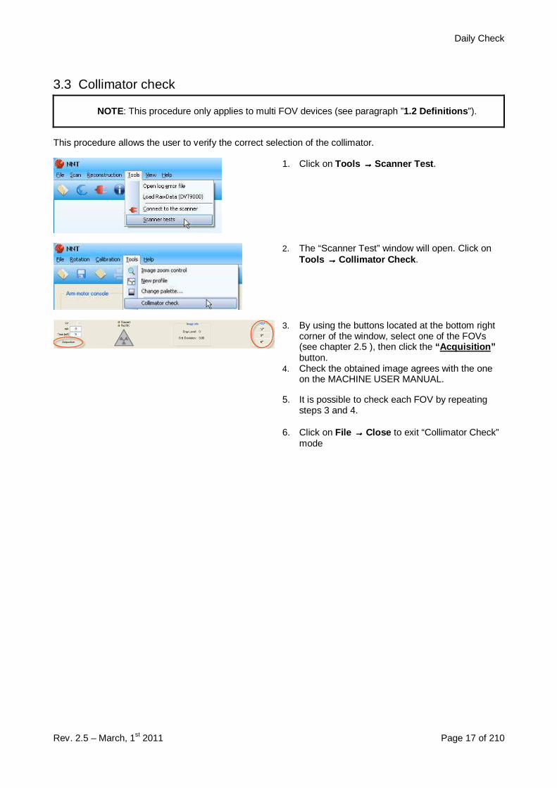
3.3 Collimator check
NOTE: This procedure only applies to multi FOV devices (see paragraph ”1.2 Definitions ”).
This procedure allows the user to verify the correct selection of the collimator.
1. Click on Tools →→→→ Scanner Test .
2. The “Scanner Test” window will open. Click onTools →→→→ Collimator Check .
3. By using the buttons located at the bottom rightcorner of the window, select one of the FOVs(see chapter 2.5 ), then click the “Acquisition”button.
4. Check the obtained image agrees with the oneon the MACHINE USER MANUAL.
5. It is possible to check each FOV by repeatingsteps 3 and 4.
6. Click on File →→→→ Close to exit “Collimator Check”mode
Blank acquisition
Rev. 2.5 – March, 1st 2011 Page 18 of 210
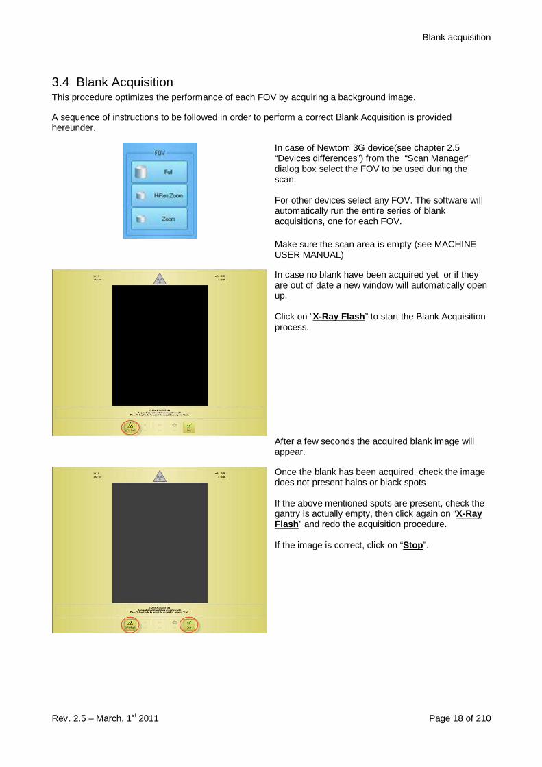
3.4 Blank AcquisitionThis procedure optimizes the performance of each FOV by acquiring a background image.
A sequence of instructions to be followed in order to perform a correct Blank Acquisition is providedhereunder.
In case of Newtom 3G device(see chapter 2.5“Devices differences”) from the “Scan Manager”dialog box select the FOV to be used during thescan.
For other devices select any FOV. The software willautomatically run the entire series of blankacquisitions, one for each FOV.
Make sure the scan area is empty (see MACHINEUSER MANUAL)
In case no blank have been acquired yet or if theyare out of date a new window will automatically openup.
Click on “X-Ray Flash ” to start the Blank Acquisitionprocess.
After a few seconds the acquired blank image willappear.
Once the blank has been acquired, check the imagedoes not present halos or black spots
If the above mentioned spots are present, check thegantry is actually empty, then click again on “X-RayFlash ” and redo the acquisition procedure.
If the image is correct, click on “Stop ”.

Scanning a patient
Rev. 2.5 – March, 1st 2011 Page 19 of 210
4 ScanningThis chapter deals with the procedures to be followed in order to get a patient’s scan.See MACHINE USER MANUAL for the instructions on patient’s positioning.
4.1 Scanning a patient
4.1.1 Selecting the FOV for scanning
At the end of the patient’s positioning, it is possible to start the scan.
Select a FOV on the FOV dialog box (see chapter 2.5“Devices differences”)
If the FOV is different from the one previouslyselected, it could be asked to perform a BlankAcquisition (see chapter 3.4 “Blank Acquisition”).
To start a scan click on Scan →→→→ Patient scan .
If a scan option choice is available (see chapter 2.5“Devices differences”), select the preferred option onthe “Choose scan option” window.
(Regular Scan: default option, reduced scan time andexposure time.Enhanced Scan: improved image quality, increasedscan and exposure time.)
Scanning a patient
Rev. 2.5 – March, 1st 2011 Page 20 of 210
4.1.2 Entering a patient’s data
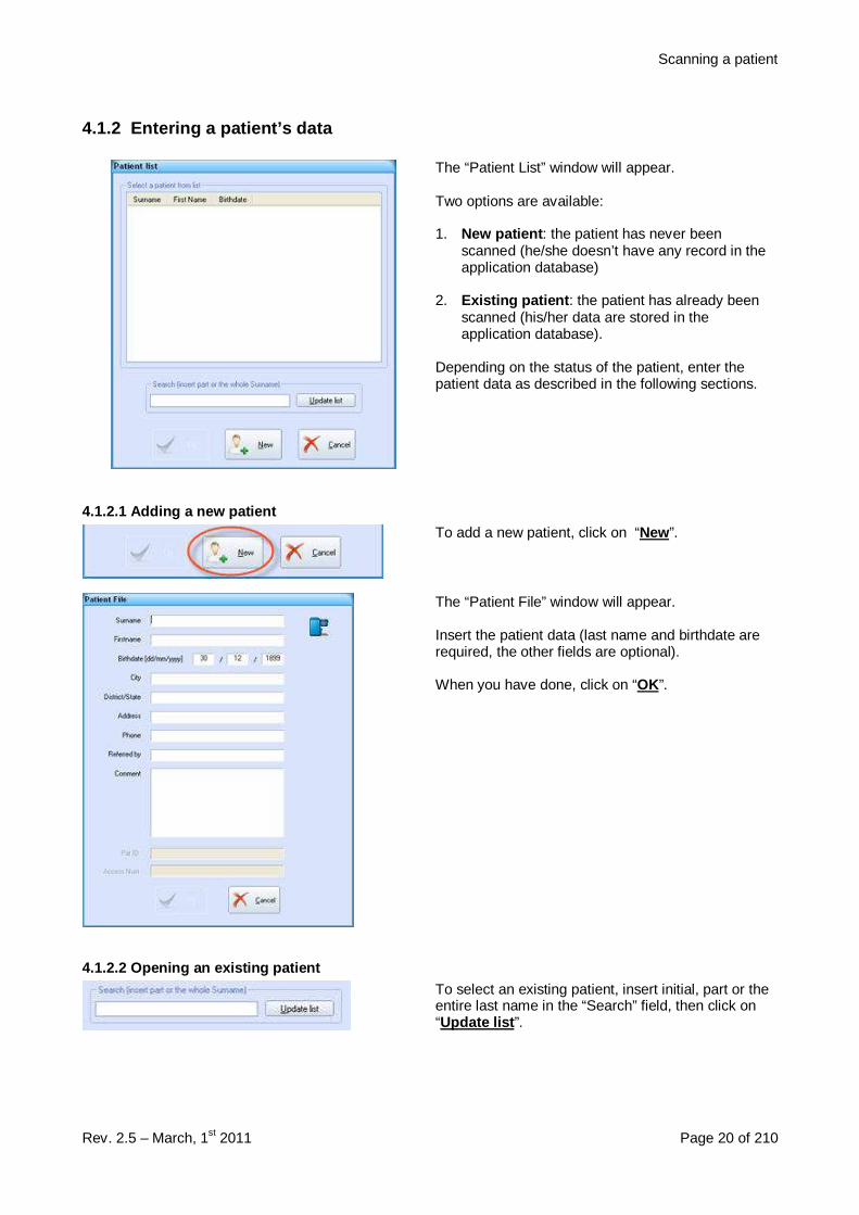
The “Patient List” window will appear.
Two options are available:
1. New patient : the patient has never beenscanned (he/she doesn’t have any record in theapplication database)
2. Existing patient : the patient has already beenscanned (his/her data are stored in theapplication database).
Depending on the status of the patient, enter thepatient data as described in the following sections.
4.1.2.1 Adding a new patientTo add a new patient, click on “New”.
The “Patient File” window will appear.
Insert the patient data (last name and birthdate arerequired, the other fields are optional).
When you have done, click on “OK”.
4.1.2.2 Opening an existing patientTo select an existing patient, insert initial, part or theentire last name in the “Search” field, then click on“Update list ”.
Scanning a patient
Rev. 2.5 – March, 1st 2011 Page 21 of 210
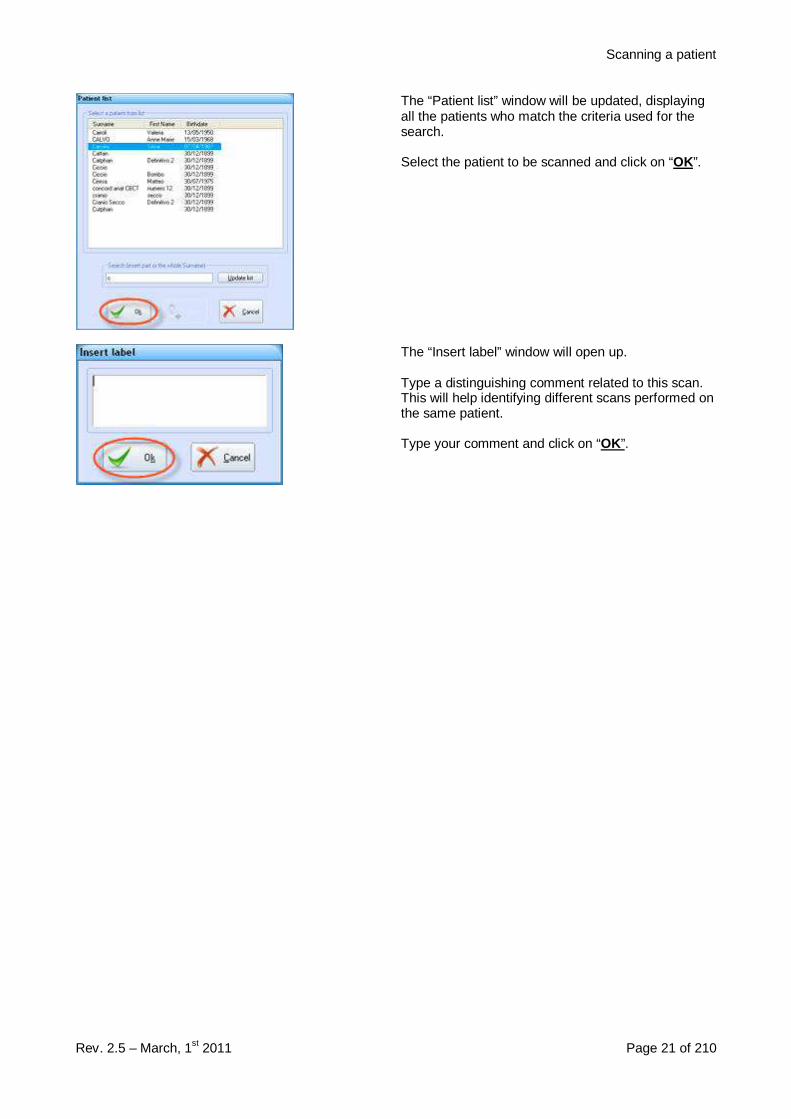
The “Patient list” window will be updated, displayingall the patients who match the criteria used for thesearch.
Select the patient to be scanned and click on “OK”.
The “Insert label” window will open up.
Type a distinguishing comment related to this scan.This will help identifying different scans performed onthe same patient.
Type your comment and click on “OK”.

Scanning a patient
Rev. 2.5 – March, 1st 2011 Page 22 of 210
4.1.3 Positioning the patient and running the scanAfter the patient’s data have been entered, thefollowing two windows will briefly appear.
The first one points out the memory to be used forthe scan has been initialized.
The second one points out the rotating arm is movingto the starting position.
At the end of the process a new window will appear.Now it is possible to place the patient into the scanarea (see MACHINE USER MANUAL).
Once the patient has been placed, go back to theMAIN WORKSTATION and click on “Next ”.
Click on “X-Ray Flash ”.
Scanning a patient
Rev. 2.5 – March, 1st 2011 Page 23 of 210
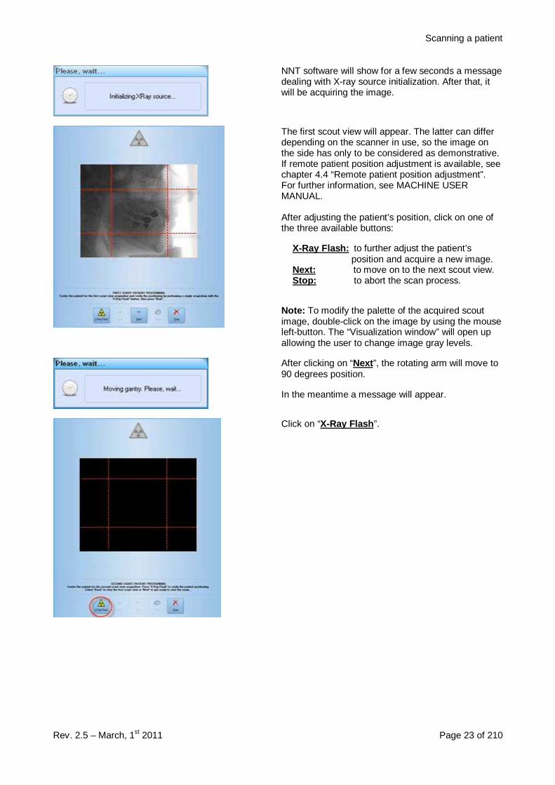
NNT software will show for a few seconds a messagedealing with X-ray source initialization. After that, itwill be acquiring the image.
The first scout view will appear. The latter can differdepending on the scanner in use, so the image onthe side has only to be considered as demonstrative.If remote patient position adjustment is available, seechapter 4.4 “Remote patient position adjustment”.For further information, see MACHINE USERMANUAL.
After adjusting the patient’s position, click on one ofthe three available buttons:
X-Ray Flash: to further adjust the patient’sposition and acquire a new image.
Next: to move on to the next scout view.Stop: to abort the scan process.
Note: To modify the palette of the acquired scoutimage, double-click on the image by using the mouseleft-button. The “Visualization window” will open upallowing the user to change image gray levels.
After clicking on “Next ”, the rotating arm will move to90 degrees position.
In the meantime a message will appear.
Click on “X-Ray Flash ”.
Scanning a patient
Rev. 2.5 – March, 1st 2011 Page 24 of 210
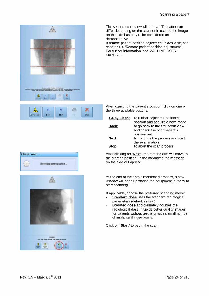
The second scout view will appear. The latter candiffer depending on the scanner in use, so the imageon the side has only to be considered asdemonstrative.If remote patient position adjustment is available, seechapter 4.4 “Remote patient position adjustment”.For further information, see MACHINE USERMANUAL.
After adjusting the patient’s position, click on one ofthe three available buttons:
X-Ray Flash: to further adjust the patient’sposition and acquire a new image.
Back: to go back to the first scout viewand check the prior patient’sposition out.
Next: to continue the process and startthe examination.
Stop: to abort the scan process.
After clicking on “Next ”, the rotating arm will move tothe starting position. In the meantime the messageon the side will appear.
At the end of the above mentioned process, a newwindow will open up stating the equipment is ready tostart scanning.
If applicable, choose the preferred scanning mode:- Standard dose uses the standard radiological
parameters (default setting)- Boosted dose approximately doubles the
radiological dose; it yields better quality imagesfor patients without teeths or with a small numberof implants/fillings/crowns.
Click on “Start ” to begin the scan.

Scanning a patient
Rev. 2.5 – March, 1st 2011 Page 25 of 210
A progress dialog box will open up showing thepercentage of the completed scan process.
Note: during the scan, it is recommended to informthe patient on the scan process status (e.g.: we areone-quarter done with the scan, one half done…,etc.)
At this point the acquired data will be manually or automatically managed depending on the currentconfiguration (see chapter 2.5 “Devices differences”).
4.1.3.1 Manual managementIn case of manual management of the RawData at theend of the scan the Raw Data window will automaticallyopen.
Refer to chapter 5 “Running a Primary Reconstruction“to get a panoramic of all available functions.
4.1.3.2 Automatic managementIf the Primary Reconstruction planning is not expected thereconstruction will automatically start. (Please refere tothe MACHINE USER MANUAL for further information.)Once the process is finished the “Visualization window”will appear, allowing to adjust the palette of the slicesgenerated by the primary reconstruction process.After the palette has been adjusted the volumetricwindow will automatically open (refere to chapter “6Volumetric Data “).To modify the automatic reconstruction parameters referto paragraph 5.5.1 “Procedure for devices with automaticreconstruction“In case the reconstruction has not successfullycompleted, at the software start up the “Recover scanmanager” window wil appear allowing to run thereconstruction in a second time (vedi capitolo 5.9“Management of non reconstructed scan” )
Scanning a patient
Rev. 2.5 – March, 1st 2011 Page 26 of 210
4.2 Scanning a denture
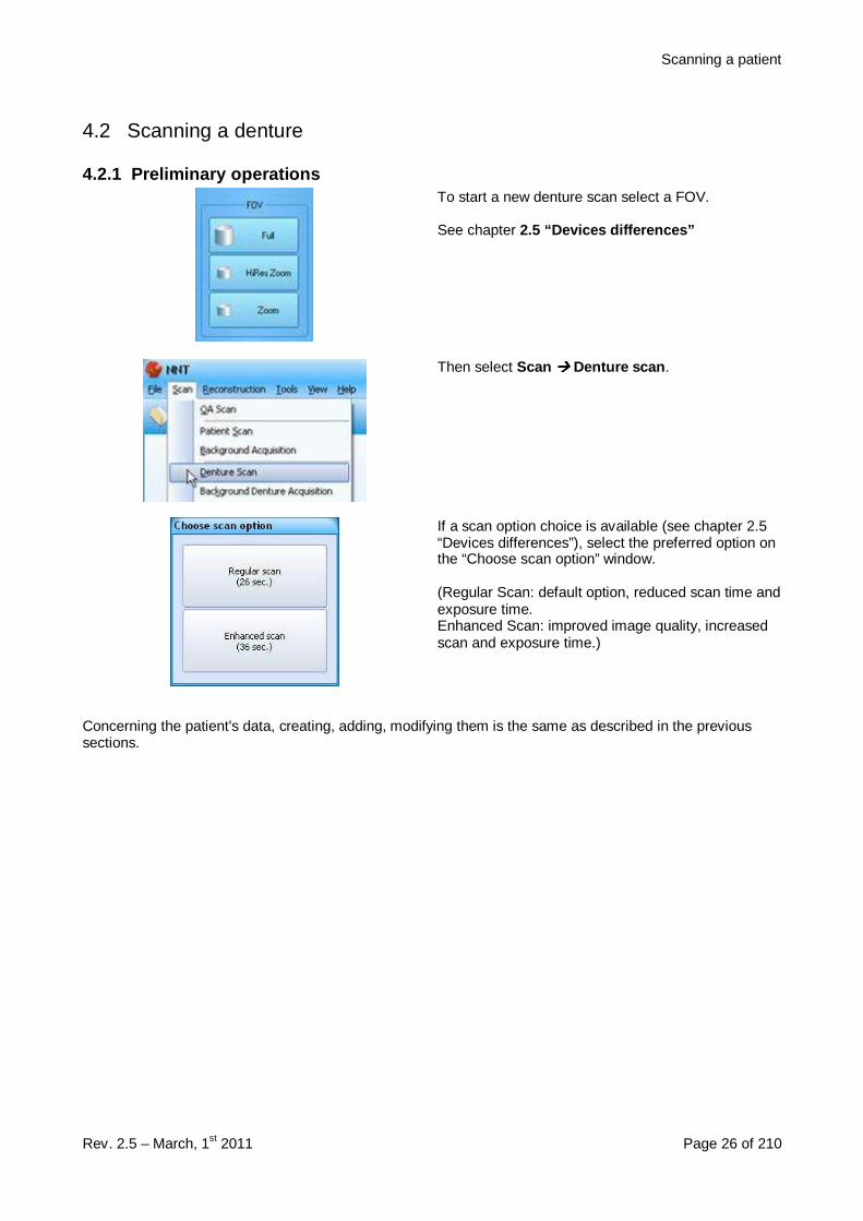
4.2.1 Preliminary operationsTo start a new denture scan select a FOV.
See chapter 2.5 “Devices differences”
Then select Scan ���� Denture scan .
If a scan option choice is available (see chapter 2.5“Devices differences”), select the preferred option onthe “Choose scan option” window.
(Regular Scan: default option, reduced scan time andexposure time.Enhanced Scan: improved image quality, increasedscan and exposure time.)
Concerning the patient's data, creating, adding, modifying them is the same as described in the previoussections.
Scanning a patient
Rev. 2.5 – March, 1st 2011 Page 27 of 210
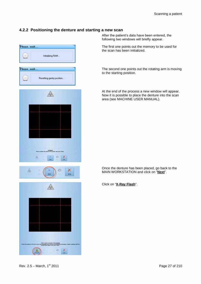
4.2.2 Positioning the denture and starting a new s canAfter the patient’s data have been entered, thefollowing two windows will briefly appear.
The first one points out the memory to be used forthe scan has been initialized.
The second one points out the rotating arm is movingto the starting position.
At the end of the process a new window will appear.Now it is possible to place the denture into the scanarea (see MACHINE USER MANUAL).
Once the denture has been placed, go back to theMAIN WORKSTATION and click on “Next ”.
Click on “X-Ray Flash ”.
Scanning a patient
Rev. 2.5 – March, 1st 2011 Page 28 of 210
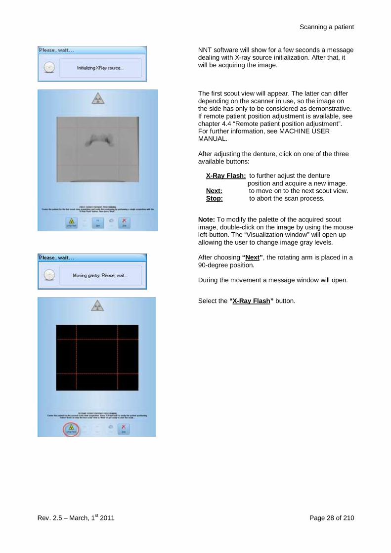
NNT software will show for a few seconds a messagedealing with X-ray source initialization. After that, itwill be acquiring the image.
The first scout view will appear. The latter can differdepending on the scanner in use, so the image onthe side has only to be considered as demonstrative.If remote patient position adjustment is available, seechapter 4.4 “Remote patient position adjustment”.For further information, see MACHINE USERMANUAL.
After adjusting the denture, click on one of the threeavailable buttons:
X-Ray Flash: to further adjust the dentureposition and acquire a new image.
Next: to move on to the next scout view.Stop: to abort the scan process.
Note: To modify the palette of the acquired scoutimage, double-click on the image by using the mouseleft-button. The “Visualization window” will open upallowing the user to change image gray levels.
After choosing “Next” , the rotating arm is placed in a90-degree position.
During the movement a message window will open.
Select the “X-Ray Flash” button.

Scanning a patient
Rev. 2.5 – March, 1st 2011 Page 29 of 210
The second scout view will appear. This image canbe different according to the device type, this picturehas to be considered just as an example.If remote patient position adjustment is available, seechapter 4.4 “Remote patient position adjustment”.Refer to the MACHINE USER MANUALl for furtherdetails.
Once the denture position has been arranged, selectone of the buttons:
X-Ray Flash if a further image is neededBack to return to the first scout view window
to verify again the first positioningNext to go on with the scan process.Stop to stop the scan process and return to
the software main window.
After selecting “Next” , the rotating arm will be resetto the starting position, this message will bedisplayed.
Then, the window will be updated, displaying thewait-for-scan state.
Select the “Start” button to start the scan.
A progress bar will display the percentage ofcompleted scan process.
Once the scan is over, the reconstruction options in the case of a patient's scan are available. Refer to thefirst part of this chapter for details.
Scanning a patient
Rev. 2.5 – March, 1st 2011 Page 30 of 210
4.3 Scanning a patient or a denture in a third-party software enviromentNNT software allows for starting a scan procedure through proper third-party softwares. Refer to suchsoftwares manuals for informations about the management of the procedure. Regarding other steps see 4.1Scanning a patient and 4.2 Scanning a denture paragraphs.Patients data are not to be managed in NNT software with this type of scan (as this is done automatically);more, NNT software returns the scan data (tipically DICOM axials) to third-party softwares.
4.4 Remote patient position adjustmentIf the unit allows the correction of the patient position by means of the workstation (please refer to the USERMANUAL to verify whether this option is available), it is possible to perform the patient centering proceduredirectly from the Main Workstation during the scout acquisition.
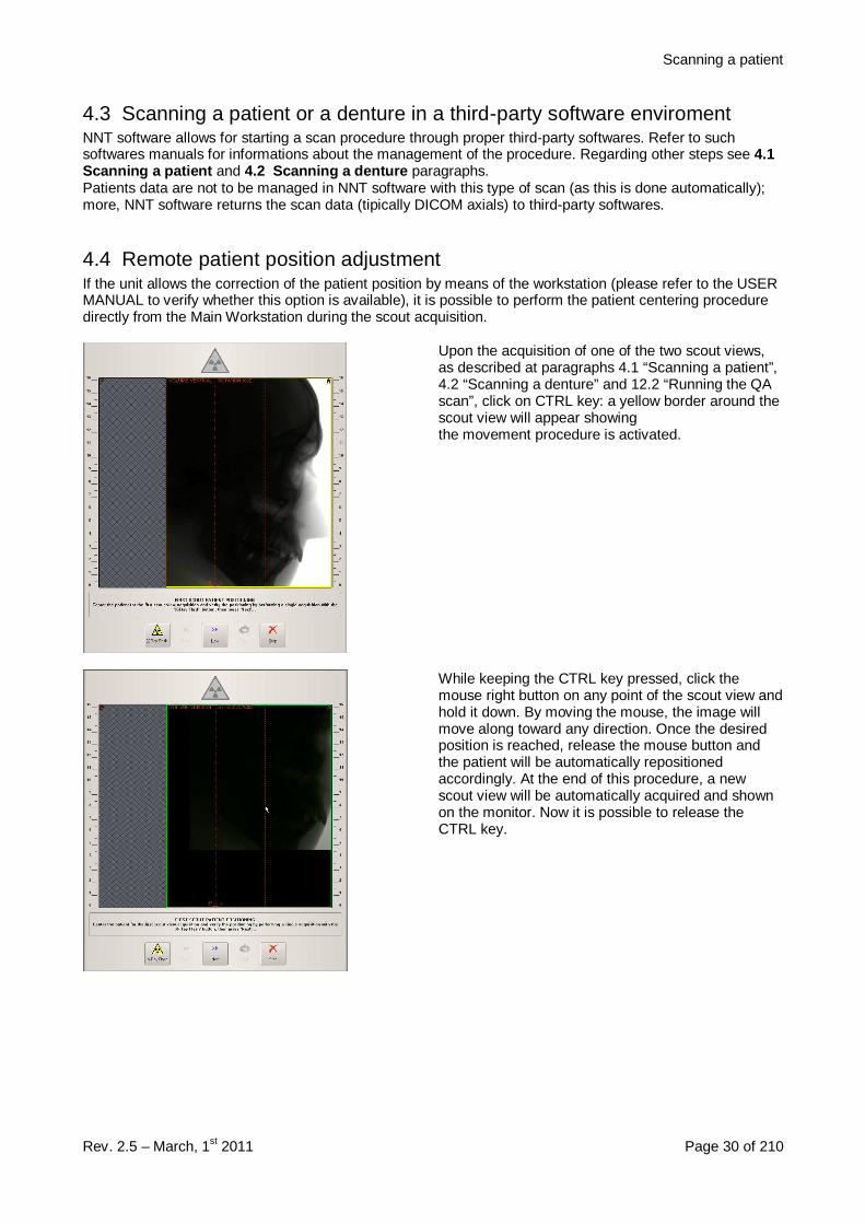
Upon the acquisition of one of the two scout views,as described at paragraphs 4.1 “Scanning a patient”,4.2 “Scanning a denture” and 12.2 “Running the QAscan”, click on CTRL key: a yellow border around thescout view will appear showingthe movement procedure is activated.
While keeping the CTRL key pressed, click themouse right button on any point of the scout view andhold it down. By moving the mouse, the image willmove along toward any direction. Once the desiredposition is reached, release the mouse button andthe patient will be automatically repositionedaccordingly. At the end of this procedure, a newscout view will be automatically acquired and shownon the monitor. Now it is possible to release theCTRL key.
Scanning a patient
Rev. 2.5 – March, 1st 2011 Page 31 of 210
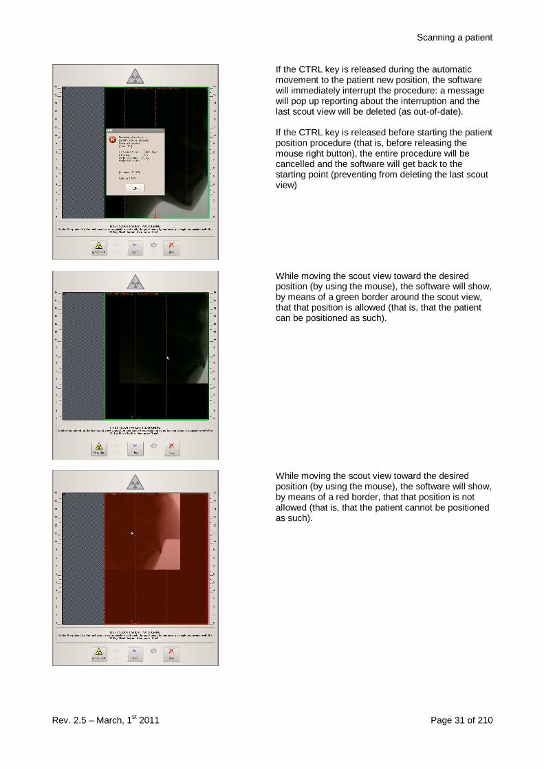
If the CTRL key is released during the automaticmovement to the patient new position, the softwarewill immediately interrupt the procedure: a messagewill pop up reporting about the interruption and thelast scout view will be deleted (as out-of-date).
If the CTRL key is released before starting the patientposition procedure (that is, before releasing themouse right button), the entire procedure will becancelled and the software will get back to thestarting point (preventing from deleting the last scoutview)
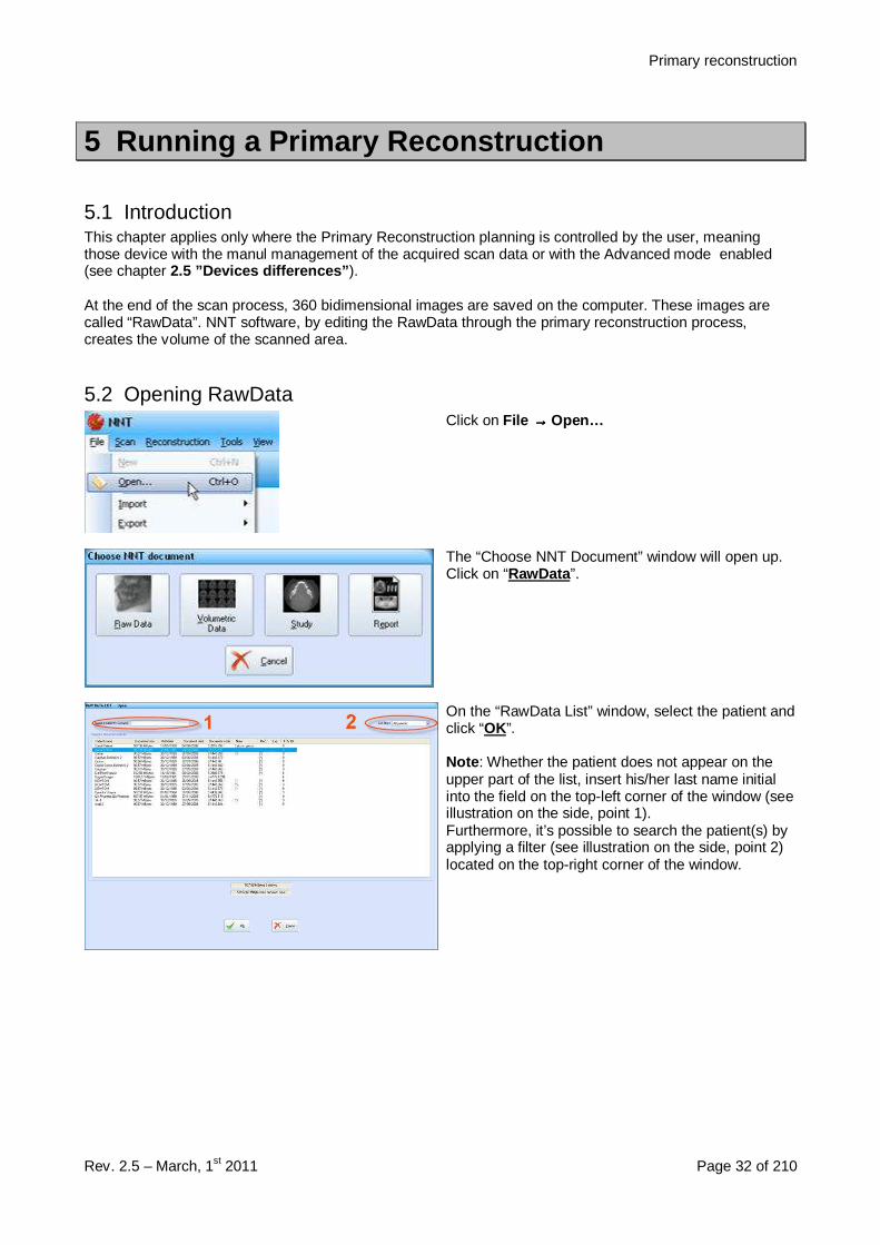
While moving the scout view toward the desiredposition (by using the mouse), the software will show,by means of a green border around the scout view,that that position is allowed (that is, that the patientcan be positioned as such).
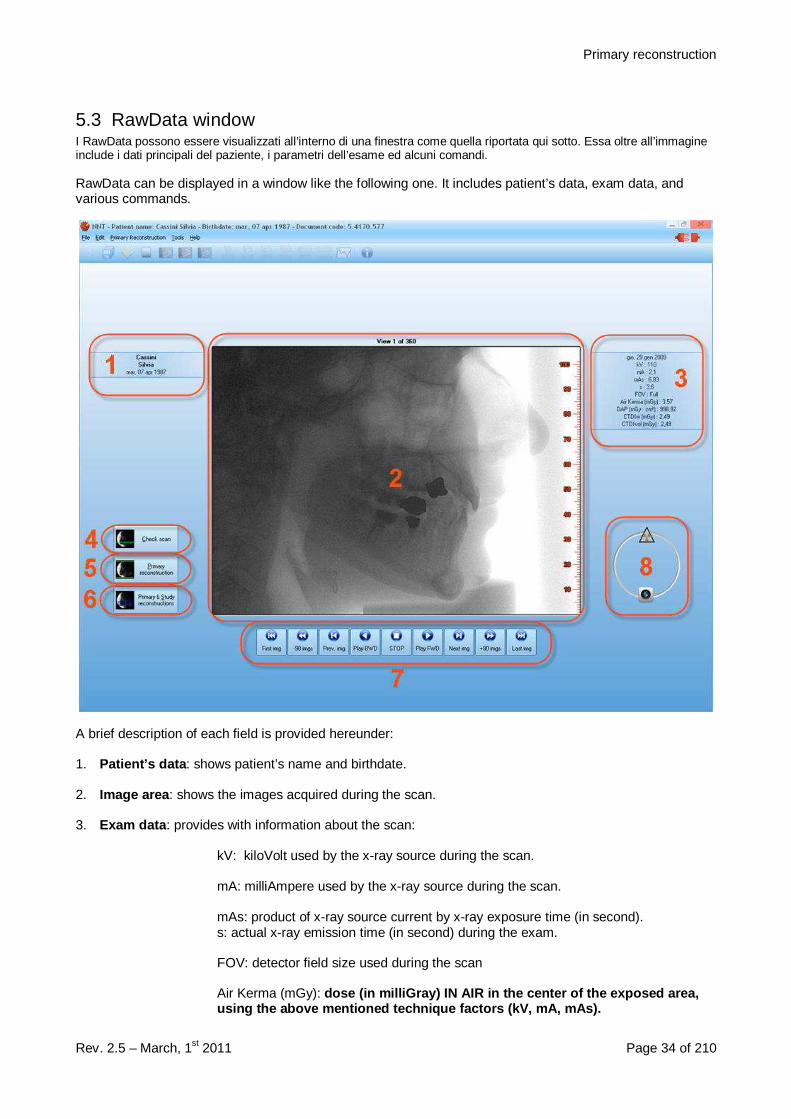
While moving the scout view toward the desiredposition (by using the mouse), the software will show,by means of a red border, that that position is notallowed (that is, that the patient cannot be positionedas such).
Primary reconstruction
Rev. 2.5 – March, 1st 2011 Page 32 of 210
5 Running a Primary Reconstruction
5.1 IntroductionThis chapter applies only where the Primary Reconstruction planning is controlled by the user, meaningthose device with the manul management of the acquired scan data or with the Advanced mode enabled(see chapter 2.5 ”Devices differences” ).
At the end of the scan process, 360 bidimensional images are saved on the computer. These images arecalled “RawData”. NNT software, by editing the RawData through the primary reconstruction process,creates the volume of the scanned area.
5.2 Opening RawDataClick on File →→→→ Open…
The “Choose NNT Document” window will open up.Click on “RawData ”.
On the “RawData List” window, select the patient andclick “OK”.
Note : Whether the patient does not appear on theupper part of the list, insert his/her last name initialinto the field on the top-left corner of the window (seeillustration on the side, point 1).Furthermore, it’s possible to search the patient(s) byapplying a filter (see illustration on the side, point 2)located on the top-right corner of the window.

Primary reconstruction
Rev. 2.5 – March, 1st 2011 Page 33 of 210
The main RawData window will open up showing thefirst image of the scan.
Primary reconstruction
Rev. 2.5 – March, 1st 2011 Page 34 of 210
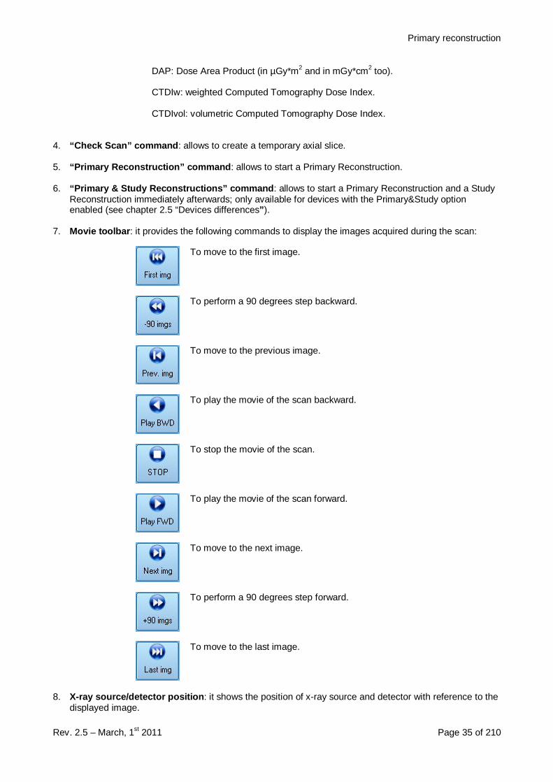
5.3 RawData windowI RawData possono essere visualizzati all’interno di una finestra come quella riportata qui sotto. Essa oltre all’immagineinclude i dati principali del paziente, i parametri dell’esame ed alcuni comandi.
RawData can be displayed in a window like the following one. It includes patient’s data, exam data, andvarious commands.
A brief description of each field is provided hereunder:
1. Patient’s data : shows patient’s name and birthdate.
2. Image area : shows the images acquired during the scan.
3. Exam data : provides with information about the scan:
kV: kiloVolt used by the x-ray source during the scan.
mA: milliAmpere used by the x-ray source during the scan.
mAs: product of x-ray source current by x-ray exposure time (in second).s: actual x-ray emission time (in second) during the exam.
FOV: detector field size used during the scan
Air Kerma (mGy): dose (in milliGray) IN AIR in the center of the exp osed area,using the above mentioned technique factors (kV, mA , mAs).
Primary reconstruction
Rev. 2.5 – March, 1st 2011 Page 35 of 210
DAP: Dose Area Product (in µGy*m2 and in mGy*cm2 too).
CTDIw: weighted Computed Tomography Dose Index.
CTDIvol: volumetric Computed Tomography Dose Index.
4. “Check Scan” command : allows to create a temporary axial slice.
5. “Primary Reconstruction” command : allows to start a Primary Reconstruction.
6. “Primary & Study Reconstructions” command : allows to start a Primary Reconstruction and a StudyReconstruction immediately afterwards; only available for devices with the Primary&Study optionenabled (see chapter 2.5 “Devices differences” ).
7. Movie toolbar : it provides the following commands to display the images acquired during the scan:
To move to the first image.
To perform a 90 degrees step backward.
To move to the previous image.
To play the movie of the scan backward.
To stop the movie of the scan.
To play the movie of the scan forward.
To move to the next image.
To perform a 90 degrees step forward.
To move to the last image.
8. X-ray source/detector position : it shows the position of x-ray source and detector with reference to thedisplayed image.
Primary reconstruction
Rev. 2.5 – March, 1st 2011 Page 36 of 210
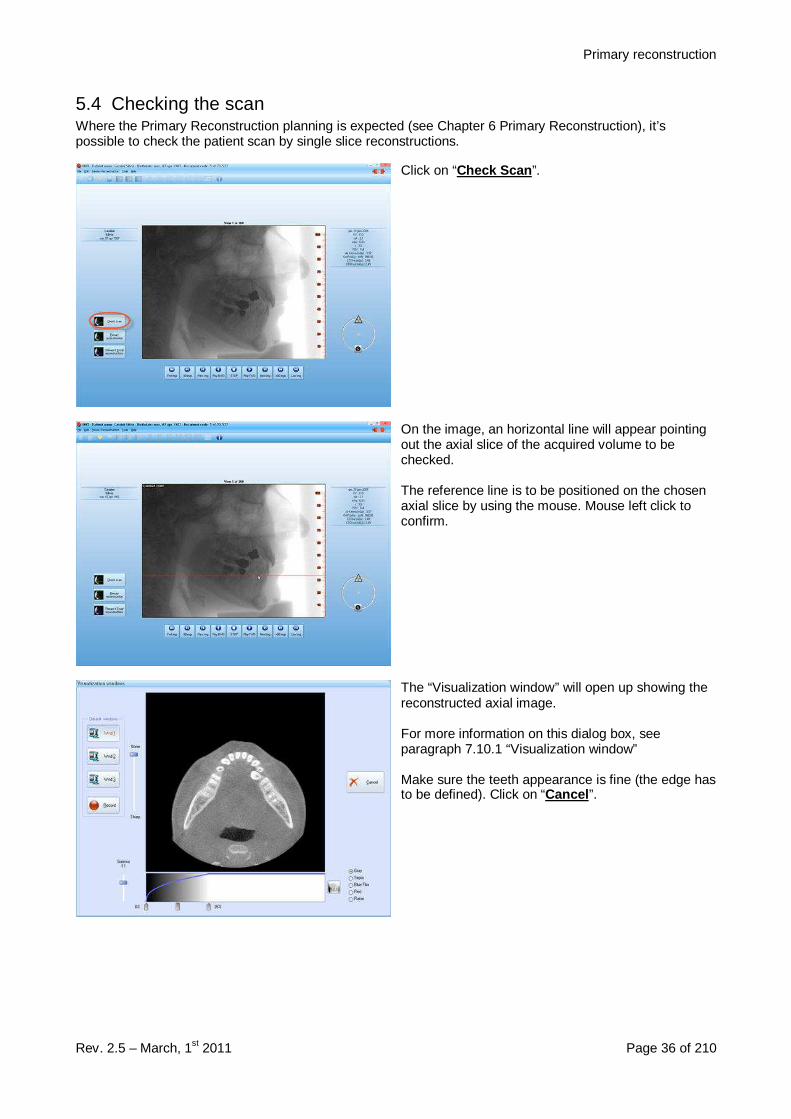
5.4 Checking the scanWhere the Primary Reconstruction planning is expected (see Chapter 6 Primary Reconstruction), it’spossible to check the patient scan by single slice reconstructions.
Click on “Check Scan ”.
On the image, an horizontal line will appear pointingout the axial slice of the acquired volume to bechecked.
The reference line is to be positioned on the chosenaxial slice by using the mouse. Mouse left click toconfirm.
The “Visualization window” will open up showing thereconstructed axial image.
For more information on this dialog box, seeparagraph 7.10.1 “Visualization window”
Make sure the teeth appearance is fine (the edge hasto be defined). Click on “Cancel ”.
Primary reconstruction
Rev. 2.5 – March, 1st 2011 Page 37 of 210
5.5 Modifying the Primary Reconstruction parametersNext are the steps to be followed in order to customize and store the default primary reconstruction settings.
The procedure differs depending on the way the system managed the Raw Data (Automatic reconstruction,Advanced mode enabbled/disabled, Primary&Study reconstruction available (see paragraph 2.5 “Devicesdifferences” ).
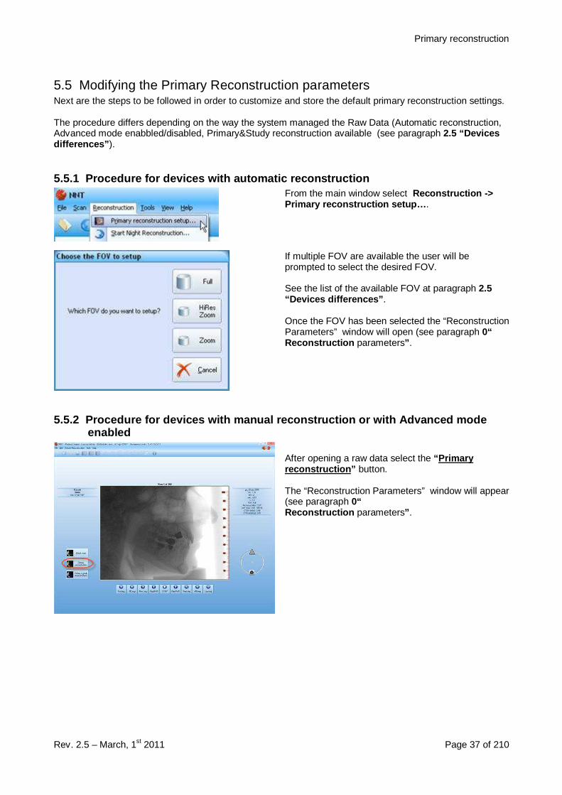
5.5.1 Procedure for devices with automatic reconst ructionFrom the main window select Reconstruction ->Primary reconstruction setup… .
If multiple FOV are available the user will beprompted to select the desired FOV.
See the list of the available FOV at paragraph 2.5“Devices differences” .
Once the FOV has been selected the “ReconstructionParameters” window will open (see paragraph 0“Reconstruction parameters” .
5.5.2 Procedure for devices with manual reconstruc tion or with Advanced modeenabled
After opening a raw data select the “Primaryreconstruction” button.
The “Reconstruction Parameters” window will appear(see paragraph 0“Reconstruction parameters” .
Primary reconstruction
Rev. 2.5 – March, 1st 2011 Page 38 of 210
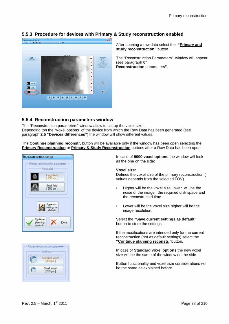
5.5.3 Procedure for devices with Primary & Study r econstruction enabled
After opening a raw data select the “Primary andstudy reconstruction” button.
The “Reconstruction Parameters” window will appear(see paragraph 0“Reconstruction parameters” .
5.5.4 Reconstruction parameters windowThe “Reconstruction parameters” window allow to set up the voxel size.Depending ton the “Voxel options” of the device from which the Raw Data has been generated (seeparagraph 2.5 “Devices differences” ) the window will show different values.
The Continue planning reconstr. button will be available only if the window has been open selecting thePrimary Reconstruction or Primary & Study Reconstruction buttons after a Raw Data has been open.
In case of 9000 voxel options the window will lookas the one on the side:
Voxel size:Defines the voxel size of the primary reconstruction (values depends from the selected FOV).
• Higher will be the voxel size, lower will be thenoise of the image, the required disk space andthe reconstructed time.
• Lower will be the voxel size higher will be theimage resolution.
Select the “Save current settings as default”button to store the settings.
If the modifications are intended only for the currentreconstruction (not as default settings) select the“Continue planning reconstr.” button.
In case of Standard voxel options the new voxelsize will be the same of the window on the side.
Button functionality and voxel size considerations willbe the same as explained before.
Primary reconstruction
Rev. 2.5 – March, 1st 2011 Page 39 of 210
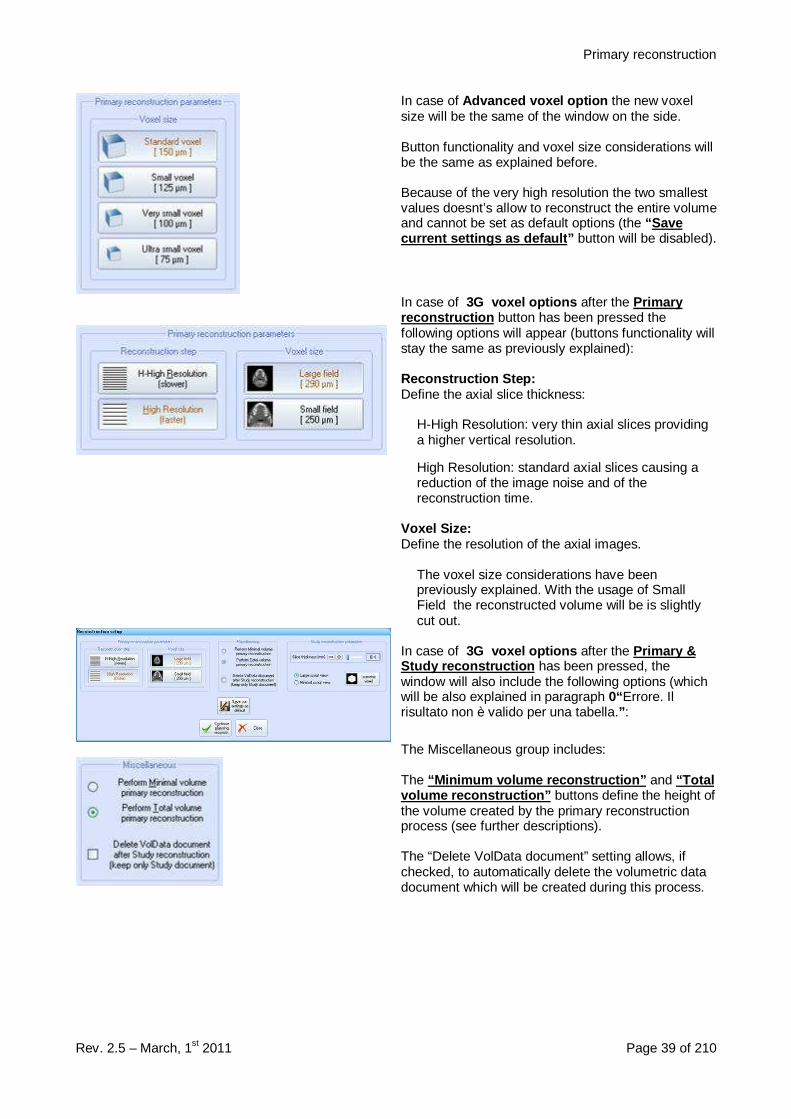
In case of Advanced voxel option the new voxelsize will be the same of the window on the side.
Button functionality and voxel size considerations willbe the same as explained before.
Because of the very high resolution the two smallestvalues doesnt’s allow to reconstruct the entire volumeand cannot be set as default options (the “Savecurrent settings as default ” button will be disabled).
In case of 3G voxel options after the Primaryreconstruction button has been pressed thefollowing options will appear (buttons functionality willstay the same as previously explained):
Reconstruction Step:Define the axial slice thickness:
H-High Resolution: very thin axial slices providinga higher vertical resolution.
High Resolution: standard axial slices causing areduction of the image noise and of thereconstruction time.
Voxel Size:Define the resolution of the axial images.
The voxel size considerations have beenpreviously explained. With the usage of SmallField the reconstructed volume will be is slightlycut out.
In case of 3G voxel options after the Primary &Study reconstruction has been pressed, thewindow will also include the following options (whichwill be also explained in paragraph 0“ Errore. Ilrisultato non è valido per una tabella.” :
The Miscellaneous group includes:
The “Minimum volume reconstruction” and “Totalvolume reconstruction” buttons define the height ofthe volume created by the primary reconstructionprocess (see further descriptions).
The “Delete VolData document” setting allows, ifchecked, to automatically delete the volumetric datadocument which will be created during this process.
Primary reconstruction
Rev. 2.5 – March, 1st 2011 Page 40 of 210
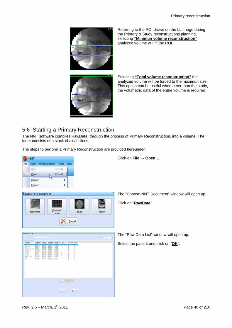
Referring to the ROI drawn on the LL image duringthe Primary & Study reconstructions planning,selecting “Minimun volume reconstruction”analyzed volume will fit the ROI.
Selecting “Total volume reconstruction” theanalyzed volume will be forced to the maximun size.This option can be useful when other than the study,the volumetric data of the entire volume is required.
5.6 Starting a Primary ReconstructionThe NNT software compiles RawData, through the process of Primary Reconstruction, into a volume. Thelatter consists of a stack of axial slices.
The steps to perform a Primary Reconstruction are provided hereunder:
Click on File →→→→ Open…
The “Choose NNT Document” window will open up.
Click on “RawData ”.
The “Raw Data List” window will open up.
Select the patient and click on “OK”.
Primary reconstruction
Rev. 2.5 – March, 1st 2011 Page 41 of 210
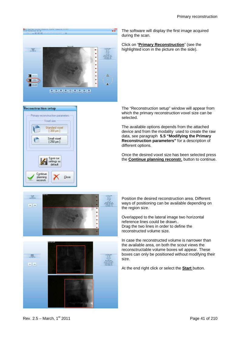
The software will display the first image acquiredduring the scan.
Click on “Primary Reconstruction ” (see thehighlighted icon in the picture on the side).
The “Reconstruction setup” window will appear fromwhich the primary reconstruction voxel size can beselected.
The available options depends from the attacheddevice and from the modality used to create the rawdata, see paragraph 5.5 “Modifying the PrimaryReconstruction parameters” for a description ofdifferent options.
Once the desired voxel size has been selected pressthe Continue planning reconstr. button to continue.
Position the desired reconstruction area. Differentways of positioning can be available depending onthe region size.
Overlapped to the lateral image two horizontalreference lines could be drawn..Drag the two lines in order to define thereconstructed volume size.
In case the reconstructed volume is narrower thanthe available area, on both the scout views thereconsctructable volume boxes wil appear. Theseboxes can only be positioned without modifying theirsize.
At the end right click or select the Start button.
Primary reconstruction
Rev. 2.5 – March, 1st 2011 Page 42 of 210
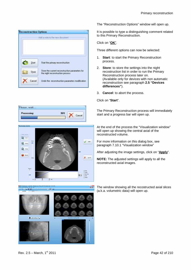
The “Reconstruction Options” window will open up.
It is possible to type a distinguishing comment relatedto this Primary Reconstruction.
Click on “OK”.
Three different options can now be selected:
1. Start : to start the Primary Reconstructionprocess.
2. Store : to store the settings into the nightrecostruction list in order to run the PrimaryReconstruction process later on.(Available only for devices with non automaticreconstruction see paragraph 2.5 “Devicesdifferences” ).
3. Cancel : to abort the process.
Click on “Start ”.
The Primary Reconstruction process will immediatelystart and a progress bar will open up.
At the end of the process the “Visualization window”will open up showing the central axial of thereconstructed volume.
For more information on this dialog box, seeparagraph 7.10.1 “Visualization window”
After adjusting the image settings, click on “Apply ”.
NOTE: The adjusted settings will apply to all thereconstructed axial images.
The window showing all the recostructed axial slices(a.k.a. volumetric data) will open up.
Primary reconstruction
Rev. 2.5 – March, 1st 2011 Page 43 of 210
5.7 Starting Primary & Study ReconstructionsThe Primary & Study Reconstructions consists of two automatic and consecutive processes which allow theuser to create a Study directly from the RawData.This option is available only for Raw Data created by device with the Primary & study options (see paragraph2.5 “Devices differences” )The steps to perform the above mentioned process are provided hereunder:
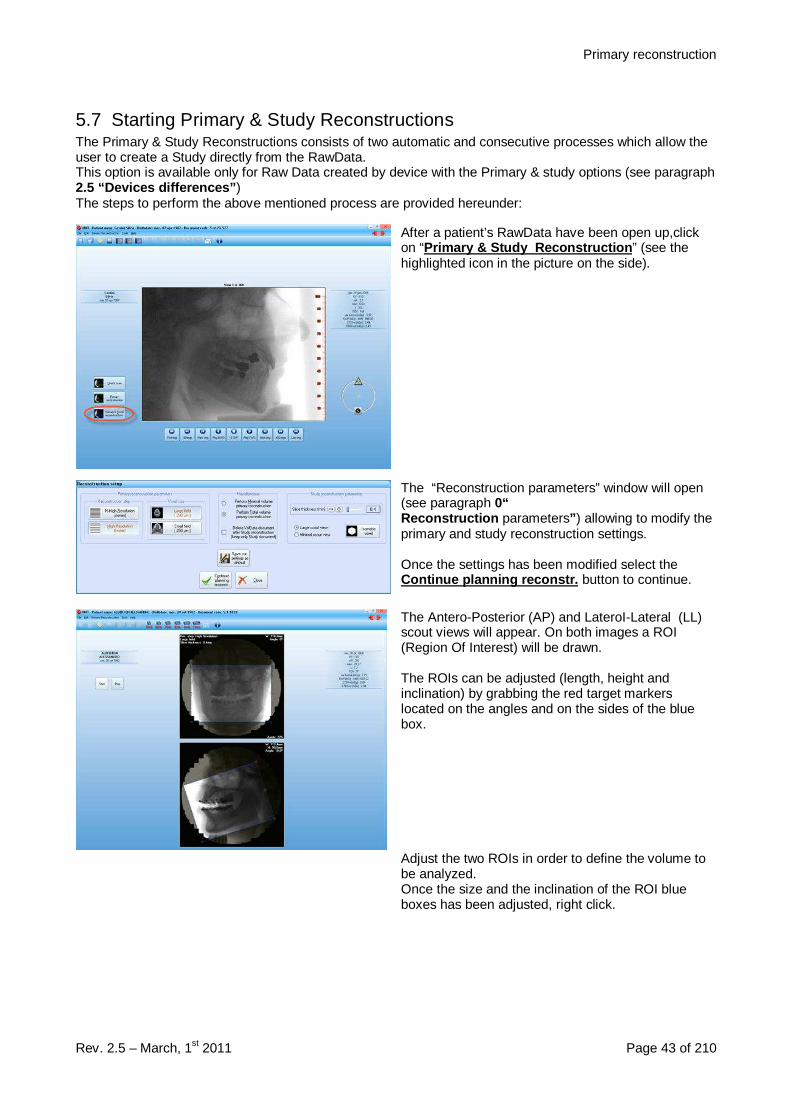
After a patient’s RawData have been open up,clickon “Primary & Study Reconstruction ” (see thehighlighted icon in the picture on the side).
The “Reconstruction parameters” window will open(see paragraph 0“Reconstruction parameters” ) allowing to modify theprimary and study reconstruction settings.
Once the settings has been modified select theContinue planning reconstr. button to continue.
The Antero-Posterior (AP) and LateroI-Lateral (LL)scout views will appear. On both images a ROI(Region Of Interest) will be drawn.
The ROIs can be adjusted (length, height andinclination) by grabbing the red target markerslocated on the angles and on the sides of the bluebox.
Adjust the two ROIs in order to define the volume tobe analyzed.Once the size and the inclination of the ROI blueboxes has been adjusted, right click.

Primary reconstruction
Rev. 2.5 – March, 1st 2011 Page 44 of 210
The “Reconstruction Options” dialog box will open up.
It is possible to type a distinguishing comment relatedto these Primary and Study Reconstructions.
1. Start : to start the Primary Reconstructionprocess.
4. Store : to store the settings into the nightrecostruction list in order to run the PrimaryReconstruction process later on. (Available onlyfor devices with non automatic reconstruction seeparagraph 2.5 “Devices differences” ).
2. Cancel : to abort the process.
Click on “Start ”.
The reconstruction process will immediately start anda progress bar will open up.
At the end of the process the “Visualization window”will open up showing the central axial of thereconstructed volume.
For more information on this dialog box, seeparagraph 7.10.1 “Visualization window”.
After adjusting the image settings, click on “Apply ”.
NOTE: the adjusted settings will apply to all thereconstructed axial images.
The window showing the study will open up.
Primary reconstruction
Rev. 2.5 – March, 1st 2011 Page 45 of 210
5.8 Night ReconstructionNight Reconstruction allows to store the settings of many Primary Reconstructions which can be performedlater on.This functionality is available only for devices with non automatic reconstruction see paragraph 2.5 “Devicesdifferences” ).
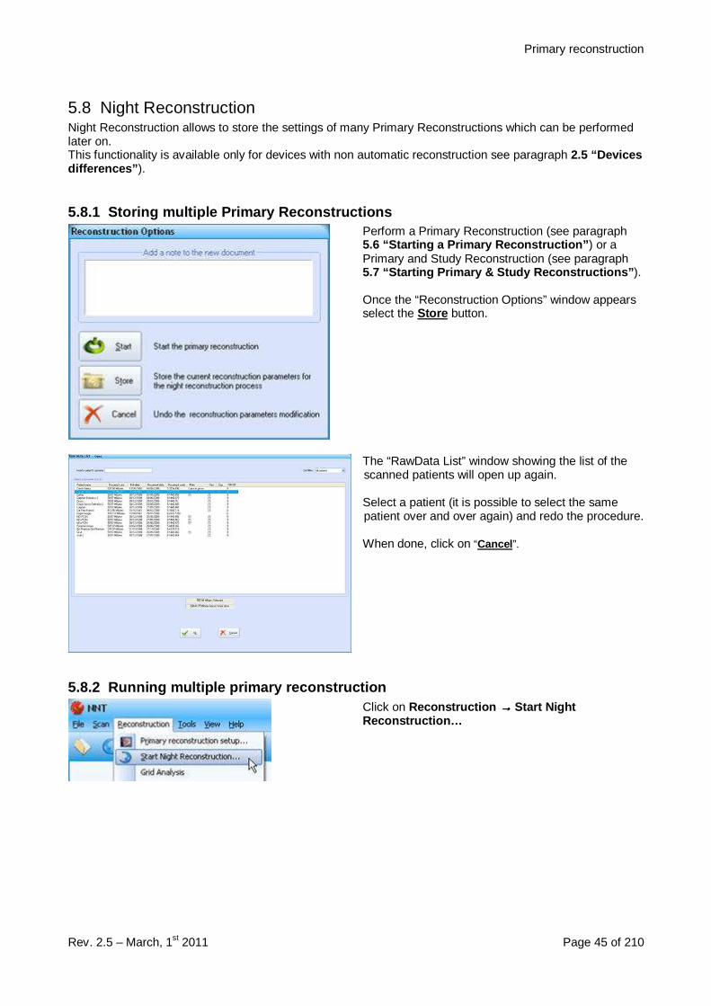
5.8.1 Storing multiple Primary ReconstructionsPerform a Primary Reconstruction (see paragraph5.6 “Starting a Primary Reconstruction” ) or aPrimary and Study Reconstruction (see paragraph5.7 “Starting Primary & Study Reconstructions” ).
Once the “Reconstruction Options” window appearsselect the Store button.
The “RawData List” window showing the list of thescanned patients will open up again.
Select a patient (it is possible to select the samepatient over and over again) and redo the procedure.
When done, click on “Cancel ”.
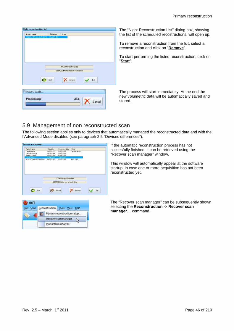
5.8.2 Running multiple primary reconstructionClick on Reconstruction →→→→ Start NightReconstruction…
Primary reconstruction
Rev. 2.5 – March, 1st 2011 Page 46 of 210
The “Night Reconstruction List” dialog box, showingthe list of the scheduled recostructions, will open up.
To remove a reconstruction from the lsit, select areconstruction and click on “Remove ”.
To start performing the listed reconstruction, click on“Start ”.
The process will start immediately. At the end thenew volumetric data will be automatically saved andstored.
5.9 Management of non reconstructed scanThe following section applies only to devices that automatically managed the reconstructed data and with thel’Advanced Mode disabled (see paragraph 2.5 “Devices differences”).
If the automatic reconstruction process has notsuccesfully finished, it can be retrieved using the“Recover scan manager” window.
This window will automatically appear at the softwarestartup, in case one or more acquisition has not beenreconstructed yet.
The “Recover scan manager” can be subsequently shownselecting the Reconstruction -> Recover scanmanager… command.
Volumetric Data
Rev. 2.5 – March, 1st 2011 Page 47 of 210
6 Volumetric Data
6.1 IntroductionAfter the Primary Reconstruction is finished a stack of axial slices has been generated. This stack of axialslices is called Volumetric Data.The axial slices that form the Volumetric Data are always horizontal.Two different views can be used to display the volumetric data: the Volumetric view and the MPR view.
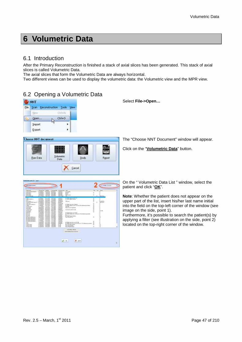
6.2 Opening a Volumetric DataSelect File->Open…
The “Choose NNT Document” window will appear.
Click on the “Volumetric Data ” button.
On the “ Volumetric Data List ” window, select thepatient and click “OK”.
Note : Whether the patient does not appear on theupper part of the list, insert his/her last name initialinto the field on the top-left corner of the window (seeimage on the side, point 1).Furthermore, it’s possible to search the patient(s) byapplying a filter (see illustration on the side, point 2)located on the top-right corner of the window.
Volumetric Data
Rev. 2.5 – March, 1st 2011 Page 48 of 210
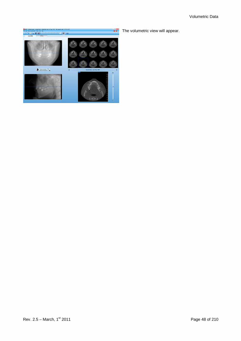
The volumetric view will appear.
Volumetric Data
Rev. 2.5 – March, 1st 2011 Page 49 of 210
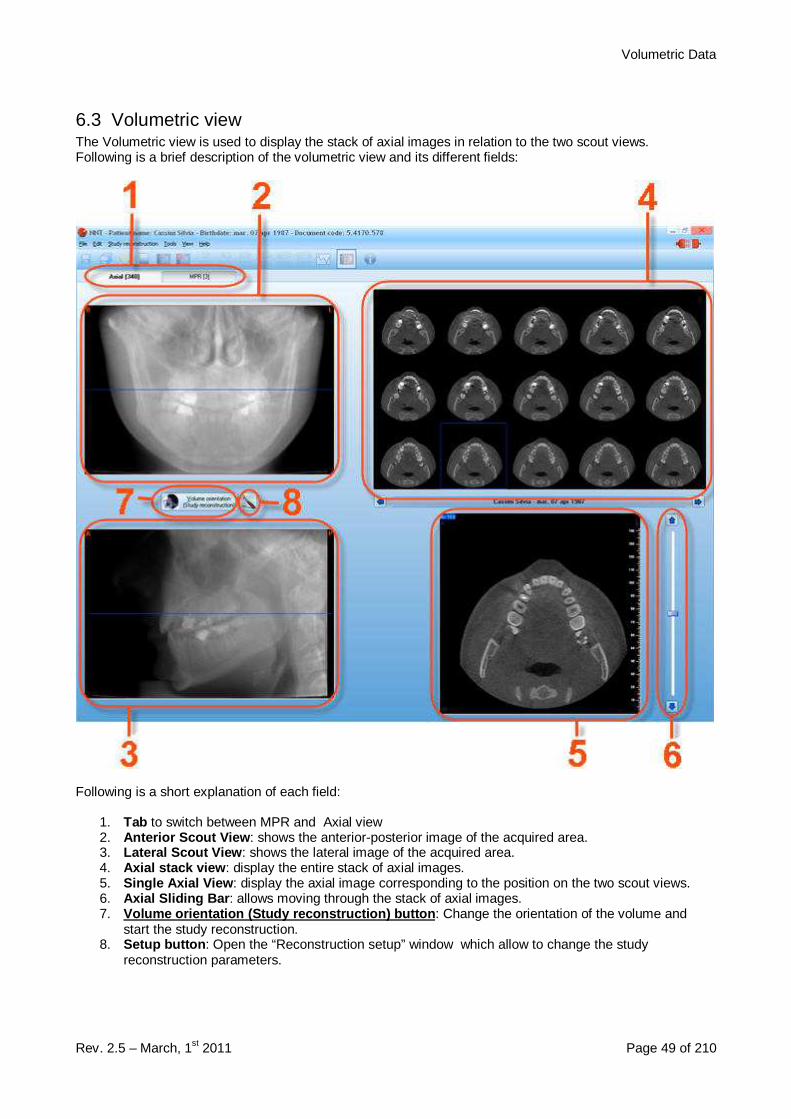
6.3 Volumetric viewThe Volumetric view is used to display the stack of axial images in relation to the two scout views.Following is a brief description of the volumetric view and its different fields:
Following is a short explanation of each field:
1. Tab to switch between MPR and Axial view2. Anterior Scout View : shows the anterior-posterior image of the acquired area.3. Lateral Scout View : shows the lateral image of the acquired area.4. Axial stack view : display the entire stack of axial images.5. Single Axial View : display the axial image corresponding to the position on the two scout views.6. Axial Sliding Bar : allows moving through the stack of axial images.7. Volume orientation (Study reconstruction) button : Change the orientation of the volume and
start the study reconstruction.8. Setup button : Open the “Reconstruction setup” window which allow to change the study
reconstruction parameters.
Volumetric Data
Rev. 2.5 – March, 1st 2011 Page 50 of 210
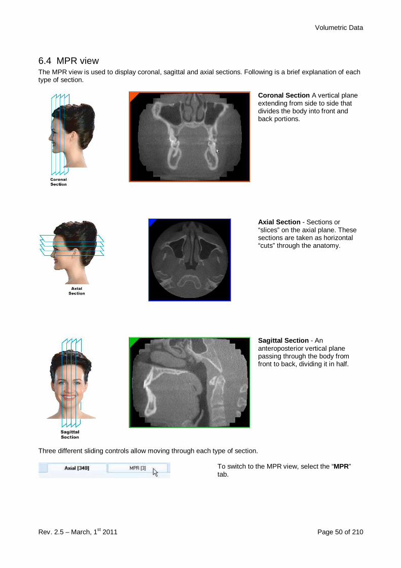
6.4 MPR viewThe MPR view is used to display coronal, sagittal and axial sections. Following is a brief explanation of eachtype of section.
Coronal Section A vertical planeextending from side to side thatdivides the body into front andback portions.
Axial Section - Sections or“slices” on the axial plane. Thesesections are taken as horizontal“cuts” through the anatomy.
Sagittal Section - Ananteroposterior vertical planepassing through the body fromfront to back, dividing it in half.
Three different sliding controls allow moving through each type of section.
To switch to the MPR view, select the “MPR”tab.
Volumetric Data
Rev. 2.5 – March, 1st 2011 Page 51 of 210
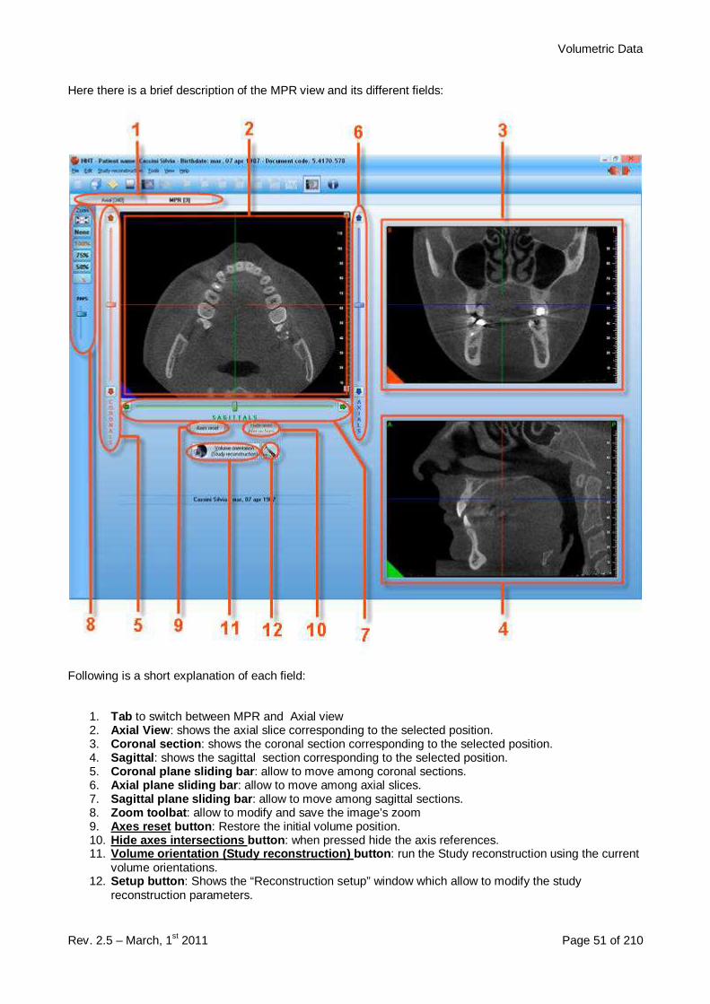
Here there is a brief description of the MPR view and its different fields:
Following is a short explanation of each field:
1. Tab to switch between MPR and Axial view2. Axial View : shows the axial slice corresponding to the selected position.3. Coronal section : shows the coronal section corresponding to the selected position.4. Sagittal : shows the sagittal section corresponding to the selected position.5. Coronal plane sliding bar : allow to move among coronal sections.6. Axial plane sliding bar : allow to move among axial slices.7. Sagittal plane sliding bar : allow to move among sagittal sections.8. Zoom toolbat : allow to modify and save the image’s zoom9. Axes reset button : Restore the initial volume position.10. Hide axes intersections button : when pressed hide the axis references.11. Volume orientation (Study reconstruction) button : run the Study reconstruction using the current
volume orientations.12. Setup button : Shows the “Reconstruction setup” window which allow to modify the study
reconstruction parameters.
Volumetric Data
Rev. 2.5 – March, 1st 2011 Page 52 of 210
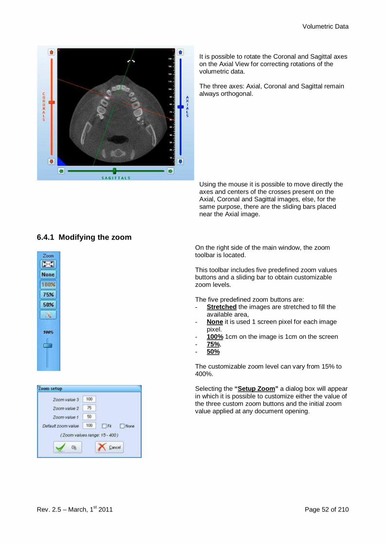
It is possible to rotate the Coronal and Sagittal axeson the Axial View for correcting rotations of thevolumetric data.
The three axes: Axial, Coronal and Sagittal remainalways orthogonal.
Using the mouse it is possible to move directly theaxes and centers of the crosses present on theAxial, Coronal and Sagittal images, else, for thesame purpose, there are the sliding bars placednear the Axial image.
6.4.1 Modifying the zoomOn the right side of the main window, the zoomtoolbar is located.
This toolbar includes five predefined zoom valuesbuttons and a sliding bar to obtain customizablezoom levels.
The five predefined zoom buttons are:- Stretched the images are stretched to fill the
available area,- None it is used 1 screen pixel for each image
pixel.- 100% 1cm on the image is 1cm on the screen- 75%,- 50%
The customizable zoom level can vary from 15% to400%.
Selecting the “Setup Zoom” a dialog box will appearin which it is possible to customize either the value ofthe three custom zoom buttons and the initial zoomvalue applied at any document opening.
Volumetric Data
Rev. 2.5 – March, 1st 2011 Page 53 of 210
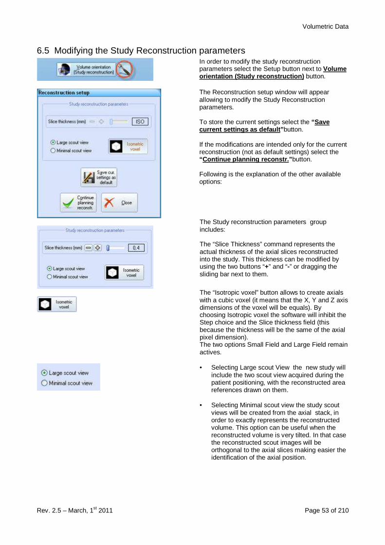
6.5 Modifying the Study Reconstruction parametersIn order to modify the study reconstructionparameters select the Setup button next to Volumeorientation (Study reconstruction) button.
The Reconstruction setup window will appearallowing to modify the Study Reconstructionparameters.
To store the current settings select the “Savecurrent settings as default” button.
If the modifications are intended only for the currentreconstruction (not as default settings) select the“Continue planning reconstr.” button.
Following is the explanation of the other availableoptions:
The Study reconstruction parameters groupincludes:
The “Slice Thickness” command represents theactual thickness of the axial slices reconstructedinto the study. This thickness can be modified byusing the two buttons “+” and “-” or dragging thesliding bar next to them.
The “Isotropic voxel” button allows to create axialswith a cubic voxel (it means that the X, Y and Z axisdimensions of the voxel will be equals). Bychoosing Isotropic voxel the software will inhibit theStep choice and the Slice thickness field (thisbecause the thickness will be the same of the axialpixel dimension).The two options Small Field and Large Field remainactives.
• Selecting Large scout View the new study willinclude the two scout view acquired during thepatient positioning, with the reconstructed areareferences drawn on them.
• Selecting Minimal scout view the study scoutviews will be created from the axial stack, inorder to exactly represents the reconstructedvolume. This option can be useful when thereconstructed volume is very tilted. In that casethe reconstructed scout images will beorthogonal to the axial slices making easier theidentification of the axial position.

Volumetric Data
Rev. 2.5 – March, 1st 2011 Page 54 of 210
6.6 Creating a new studyTo create a new study select the Volumeorientation (Study reconstruction) button.
In case the Volume orientation (Studyreconstruction) button has been selected from thevolumetric view:
A blue ROI box (Region Of Interest) will appear onboth the two scout views.
The ROI of the two images is the same area viewedfrom two different points of view.
On the axial image a blu cross will appear, itdetermines the rotation of the study respect thanthe volumetric.
On each scout image the ROI can be adjusted bygrabbing the red target markets located at thecorners of the ROI and in the middle of the borders.
On the anterior scout view the inclination, theposition and the width of the ROI can be adjusted.
On the top right corner of the image the width (inmm) and the inclination of the ROI are shown.
On the bottom right corner the amount of resultingaxial slices is displayed.
On the lateral scout view, the height, width,inclination and position of the ROI can be adjusted.
On the top right corner of the image the width andheight (in mm), and the inclination of the ROI areshown.
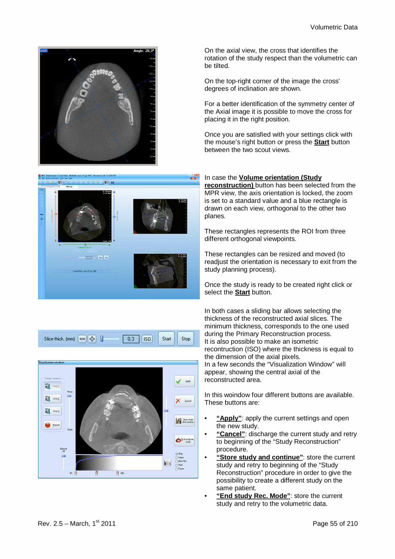
Volumetric Data
Rev. 2.5 – March, 1st 2011 Page 55 of 210
On the axial view, the cross that identifies therotation of the study respect than the volumetric canbe tilted.
On the top-right corner of the image the cross’degrees of inclination are shown.
For a better identification of the symmetry center ofthe Axial image it is possible to move the cross forplacing it in the right position.
Once you are satisfied with your settings click withthe mouse’s right button or press the Start buttonbetween the two scout views.
In case the Volume orientation (Studyreconstruction) button has been selected from theMPR view, the axis orientation is locked, the zoomis set to a standard value and a blue rectangle isdrawn on each view, orthogonal to the other twoplanes.
These rectangles represents the ROI from threedifferent orthogonal viewpoints.
These rectangles can be resized and moved (toreadjust the orientation is necessary to exit from thestudy planning process).
Once the study is ready to be created right click orselect the Start button.
In both cases a sliding bar allows selecting thethickness of the reconstructed axial slices. Theminimum thickness, corresponds to the one usedduring the Primary Reconstruction process.It is also possible to make an isometricrecontruction (ISO) where the thickness is equal tothe dimension of the axial pixels.In a few seconds the “Visualization Window” willappear, showing the central axial of thereconstructed area.
In this woindow four different buttons are available.These buttons are:
• “Apply” : apply the current settings and openthe new study.
• “Cancel” : discharge the current study and retryto beginning of the “Study Reconstruction”procedure.
• “Store study and continue” : store the currentstudy and retry to beginning of the “StudyReconstruction” procedure in order to give thepossibility to create a different study on thesame patient.
• “End study Rec. Mode” : store the currentstudy and retry to the volumetric data.
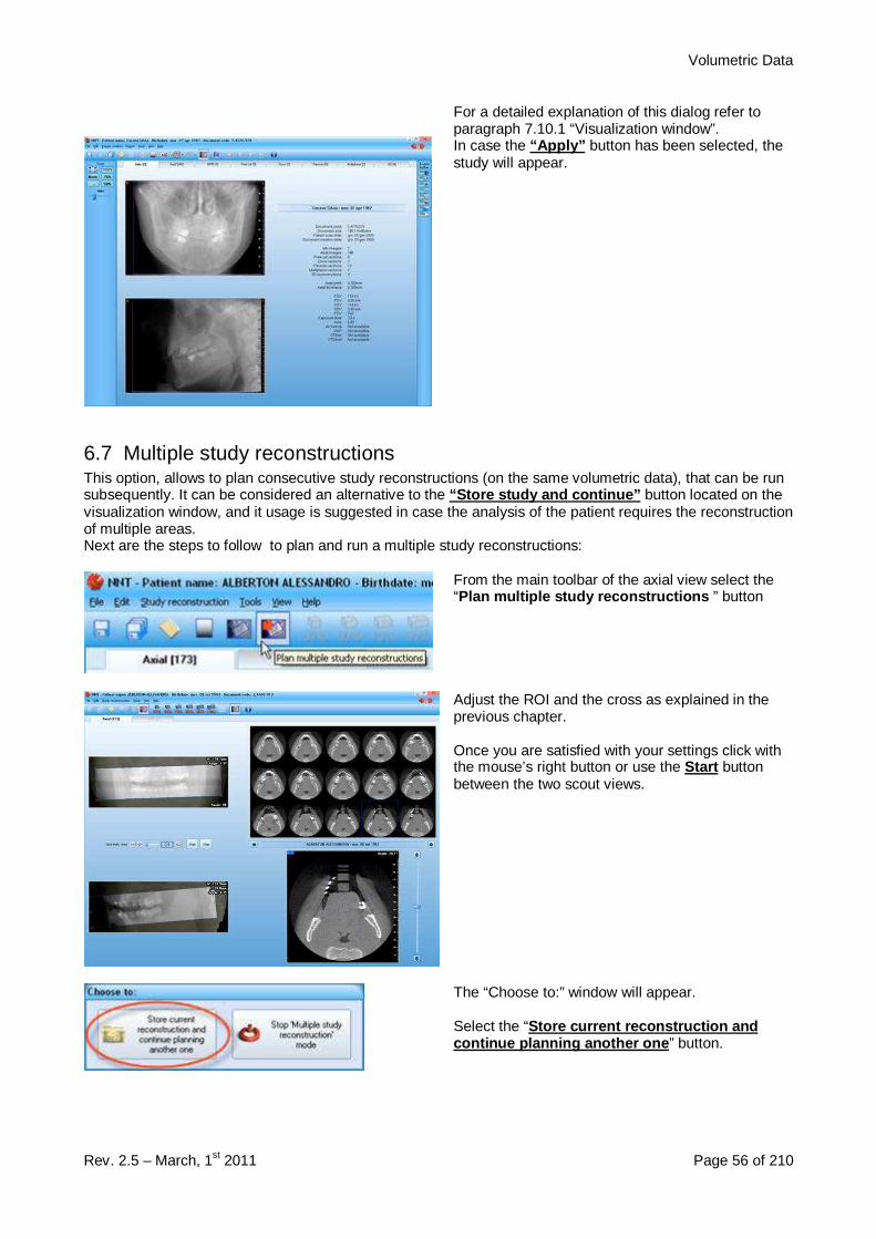
Volumetric Data
Rev. 2.5 – March, 1st 2011 Page 56 of 210
For a detailed explanation of this dialog refer toparagraph 7.10.1 “Visualization window”.In case the “Apply” button has been selected, thestudy will appear.
6.7 Multiple study reconstructionsThis option, allows to plan consecutive study reconstructions (on the same volumetric data), that can be runsubsequently. It can be considered an alternative to the “Store study and continue” button located on thevisualization window, and it usage is suggested in case the analysis of the patient requires the reconstructionof multiple areas.Next are the steps to follow to plan and run a multiple study reconstructions:
From the main toolbar of the axial view select the“Plan multiple study reconstructions ” button
Adjust the ROI and the cross as explained in theprevious chapter.
Once you are satisfied with your settings click withthe mouse’s right button or use the Start buttonbetween the two scout views.
The “Choose to:” window will appear.
Select the “Store current reconstruction andcontinue planning another one ” button.
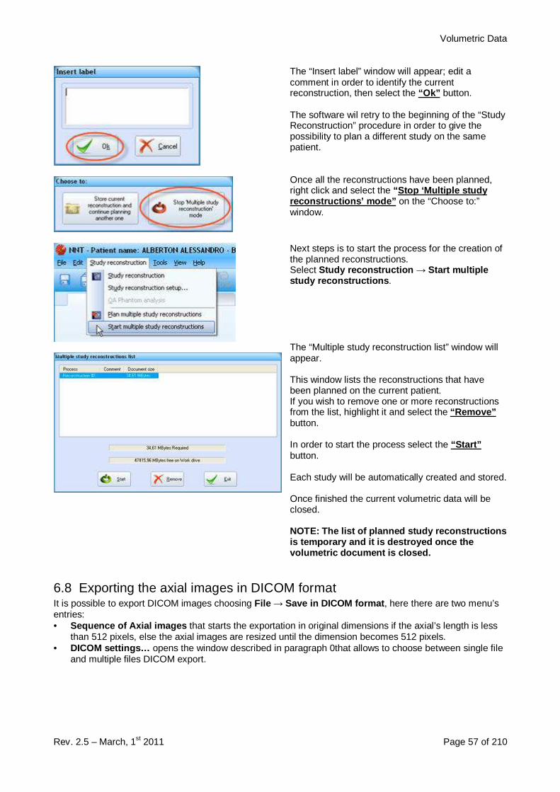
Volumetric Data
Rev. 2.5 – March, 1st 2011 Page 57 of 210
The “Insert label” window will appear; edit acomment in order to identify the currentreconstruction, then select the “Ok” button.
The software wil retry to the beginning of the “StudyReconstruction” procedure in order to give thepossibility to plan a different study on the samepatient.
Once all the reconstructions have been planned,right click and select the “Stop ‘Multiple studyreconstructions’ mode” on the “Choose to:”window.
Next steps is to start the process for the creation ofthe planned reconstructions.Select Study reconstruction → Start multiplestudy reconstructions .
The “Multiple study reconstruction list” window willappear.
This window lists the reconstructions that havebeen planned on the current patient.If you wish to remove one or more reconstructionsfrom the list, highlight it and select the “Remove”button.
In order to start the process select the “Start”button.
Each study will be automatically created and stored.
Once finished the current volumetric data will beclosed.
NOTE: The list of planned study reconstructionsis temporary and it is destroyed once thevolumetric document is closed.
6.8 Exporting the axial images in DICOM formatIt is possible to export DICOM images choosing File → Save in DICOM format , here there are two menu’sentries:• Sequence of Axial images that starts the exportation in original dimensions if the axial’s length is less
than 512 pixels, else the axial images are resized until the dimension becomes 512 pixels.• DICOM settings… opens the window described in paragraph 0that allows to choose between single file
and multiple files DICOM export.

Working with a Study
Rev. 2.5 – March, 1st 2011 Page 58 of 210
7 Working with a Study
7.1 IntroductionAfter a study has been created, it contains only the two scout views and the stack of axial images generatedfrom the ROI set up inside the Volumetric data window.
7.2 Opening a StudySelect File->Open…
The “Choose NNT Document” window will appear.
Click on the “Study ” button.
On the “ Study List ” window, select the patient andclick “OK”.
Note : Whether the patient does not appear on theupper part of the list, insert his/her last name initialinto the field on the top-left corner of the window (seeimage on the side, point 1).Furthermore, it’s possible to search the patient(s) byapplying a filter (see illustration on the side, point 2)located on the top-right corner of the window.
The study view will appear.
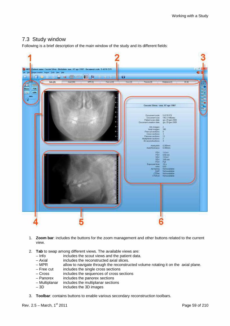
Working with a Study
Rev. 2.5 – March, 1st 2011 Page 59 of 210
7.3 Study windowFollowing is a brief description of the main window of the study and its different fields:
1. Zoom bar : includes the buttons for the zoom management and other buttons related to the currentview.
2. Tab to swap among different views. The available views are:– Info includes the scout views and the patient data.– Axial includes the reconstructed axial slices.– MPR allow to navigate through the reconstructed volume rotating it on the axial plane.– Free cut includes the single cross sections– Cross includes the sequences of cross sections– Panorex includes the panorex sections– Multiplanar includes the multiplanar sections– 3D includes the 3D images
3. Toolbar : contains buttons to enable various secondary reconstruction toolbars.
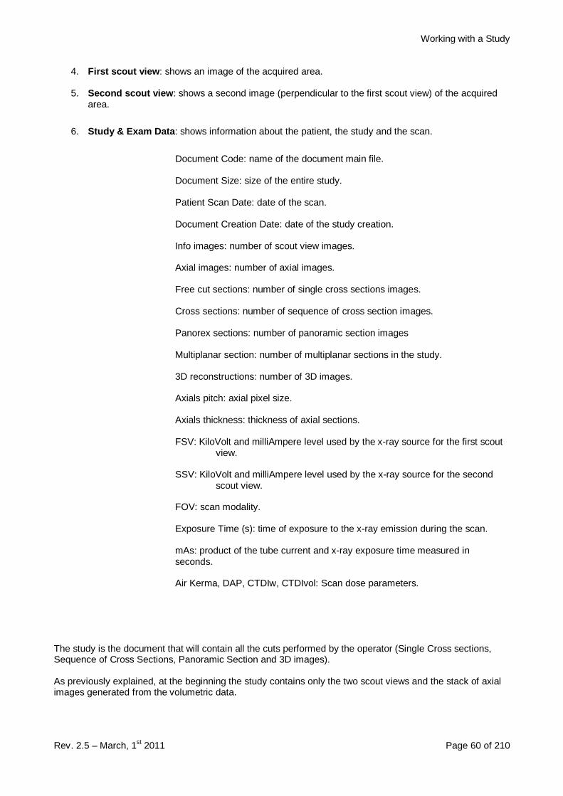
Working with a Study
Rev. 2.5 – March, 1st 2011 Page 60 of 210
4. First scout view : shows an image of the acquired area.
5. Second scout view : shows a second image (perpendicular to the first scout view) of the acquiredarea.
6. Study & Exam Data : shows information about the patient, the study and the scan.
Document Code: name of the document main file.
Document Size: size of the entire study.
Patient Scan Date: date of the scan.
Document Creation Date: date of the study creation.
Info images: number of scout view images.
Axial images: number of axial images.
Free cut sections: number of single cross sections images.
Cross sections: number of sequence of cross section images.
Panorex sections: number of panoramic section images
Multiplanar section: number of multiplanar sections in the study.
3D reconstructions: number of 3D images.
Axials pitch: axial pixel size.
Axials thickness: thickness of axial sections.
FSV: KiloVolt and milliAmpere level used by the x-ray source for the first scoutview.
SSV: KiloVolt and milliAmpere level used by the x-ray source for the secondscout view.
FOV: scan modality.
Exposure Time (s): time of exposure to the x-ray emission during the scan.
mAs: product of the tube current and x-ray exposure time measured inseconds.
Air Kerma, DAP, CTDIw, CTDIvol: Scan dose parameters.
The study is the document that will contain all the cuts performed by the operator (Single Cross sections,Sequence of Cross Sections, Panoramic Section and 3D images).
As previously explained, at the beginning the study contains only the two scout views and the stack of axialimages generated from the volumetric data.
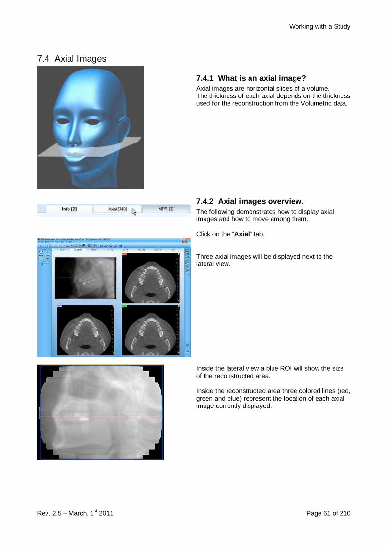
Working with a Study
Rev. 2.5 – March, 1st 2011 Page 61 of 210
7.4 Axial Images
7.4.1 What is an axial image?Axial images are horizontal slices of a volume.The thickness of each axial depends on the thicknessused for the reconstruction from the Volumetric data.
7.4.2 Axial images overview.The following demonstrates how to display axialimages and how to move among them.
Click on the “Axial ” tab.
Three axial images will be displayed next to thelateral view.
Inside the lateral view a blue ROI will show the sizeof the reconstructed area.
Inside the reconstructed area three colored lines (red,green and blue) represent the location of each axialimage currently displayed.
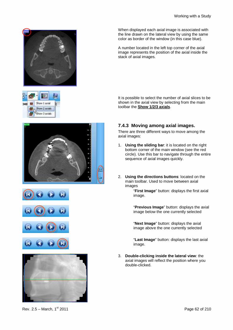
Working with a Study
Rev. 2.5 – March, 1st 2011 Page 62 of 210
When displayed each axial image is associated withthe line drawn on the lateral view by using the samecolor as border of the window (in this case blue).
A number located in the left top corner of the axialimage represents the position of the axial inside thestack of axial images.
It is possible to select the number of axial slices to beshown in the axial view by selecting from the maintoolbar the Show 1/2/3 axials .
7.4.3 Moving among axial images.There are three different ways to move among theaxial images:
1. Using the sliding bar : it is located on the rightbottom corner of the main window (see the redcircle). Use this bar to navigate through the entiresequence of axial images quickly.
2. Using the directions buttons : located on themain toolbar. Used to move between axialimages
“First Image ” button: displays the first axialimage.
“Previous Image ” button: displays the axialimage below the one currently selected
“Next Image ” button: displays the axialimage above the one currently selected
“Last Image ” button: displays the last axialimage.
3. Double-clicking inside the lateral view : theaxial images will reflect the position where youdouble-clicked.
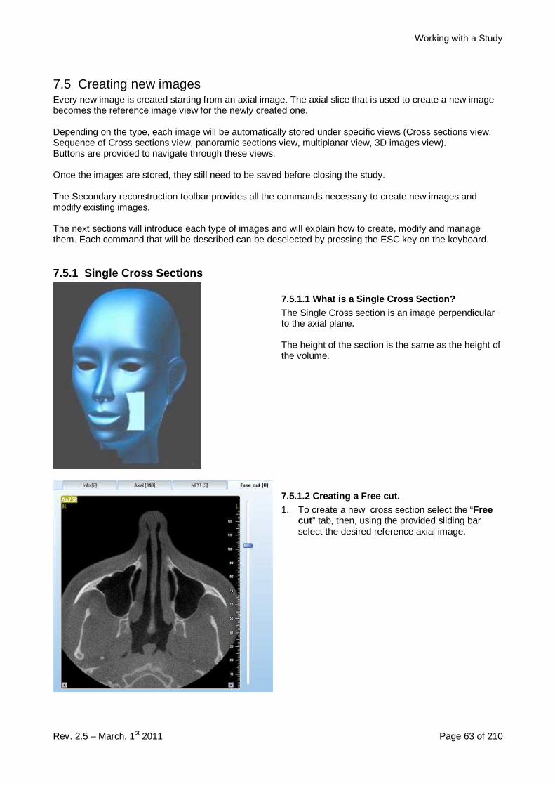
Working with a Study
Rev. 2.5 – March, 1st 2011 Page 63 of 210
7.5 Creating new imagesEvery new image is created starting from an axial image. The axial slice that is used to create a new imagebecomes the reference image view for the newly created one.
Depending on the type, each image will be automatically stored under specific views (Cross sections view,Sequence of Cross sections view, panoramic sections view, multiplanar view, 3D images view).Buttons are provided to navigate through these views.
Once the images are stored, they still need to be saved before closing the study.
The Secondary reconstruction toolbar provides all the commands necessary to create new images andmodify existing images.
The next sections will introduce each type of images and will explain how to create, modify and managethem. Each command that will be described can be deselected by pressing the ESC key on the keyboard.
7.5.1 Single Cross Sections
7.5.1.1 What is a Single Cross Section?The Single Cross section is an image perpendicularto the axial plane.
The height of the section is the same as the height ofthe volume.
7.5.1.2 Creating a Free cut.1. To create a new cross section select the “Free
cut ” tab, then, using the provided sliding barselect the desired reference axial image.
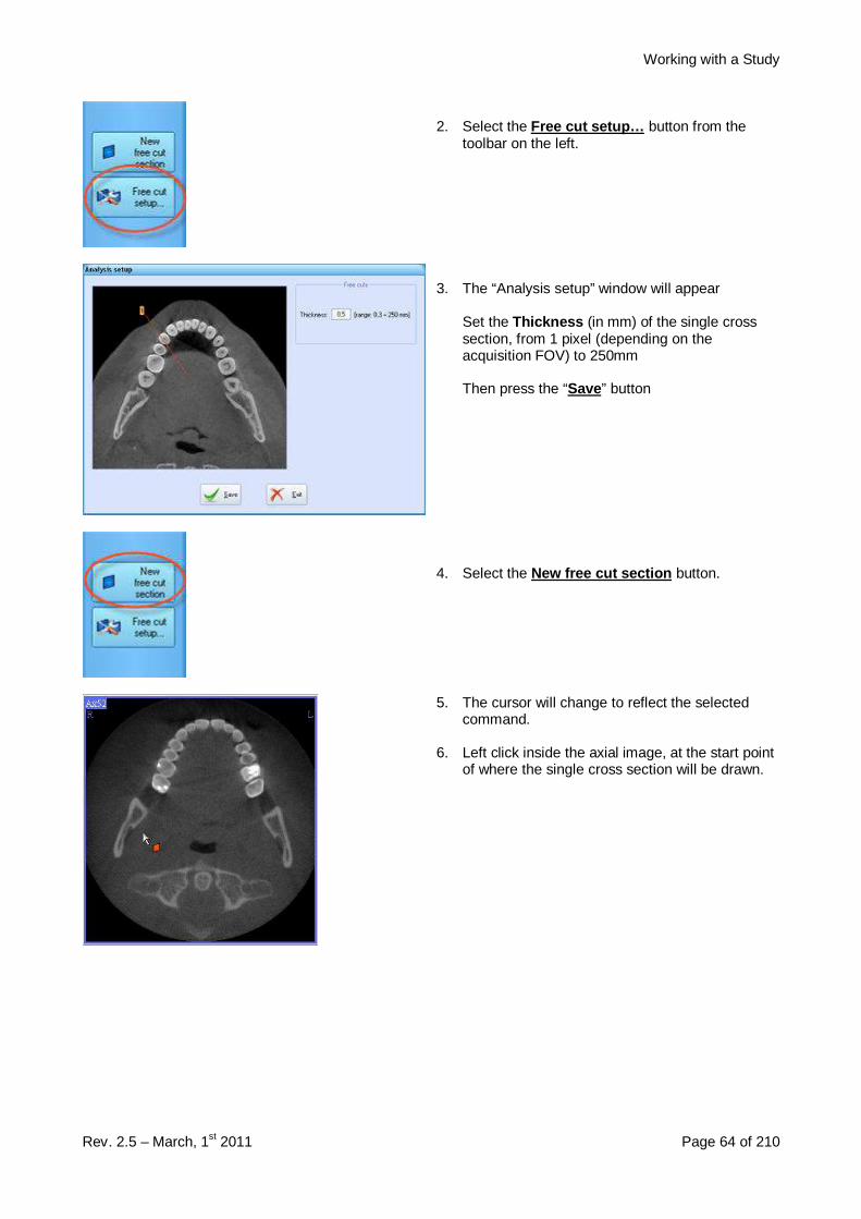
Working with a Study
Rev. 2.5 – March, 1st 2011 Page 64 of 210
2. Select the Free cut setup… button from thetoolbar on the left.
3. The “Analysis setup” window will appear
Set the Thickness (in mm) of the single crosssection, from 1 pixel (depending on theacquisition FOV) to 250mm
Then press the “Save” button
4. Select the New free cut section button.
5. The cursor will change to reflect the selectedcommand.
6. Left click inside the axial image, at the start pointof where the single cross section will be drawn.

Working with a Study
Rev. 2.5 – March, 1st 2011 Page 65 of 210
7. Drag the line to define the end point of thesection. Using the mouse wheel it is possibleto navigate through the axial images whiletracing the line.
8. Left (or right) click to set the end point of yourcross section.
9. The new image will appear beside the axial sliceused as reference image.
7.5.2 Sequence of Cross Sections
7.5.2.1 What is a Sequence of Cross Sections?The Sequence of Cross Sections is a series of singlecross sections, perpendicular to a traced path.
The height of each section is the same as the heightof the volume.
The width, thickness and distance between eachsection can vary.
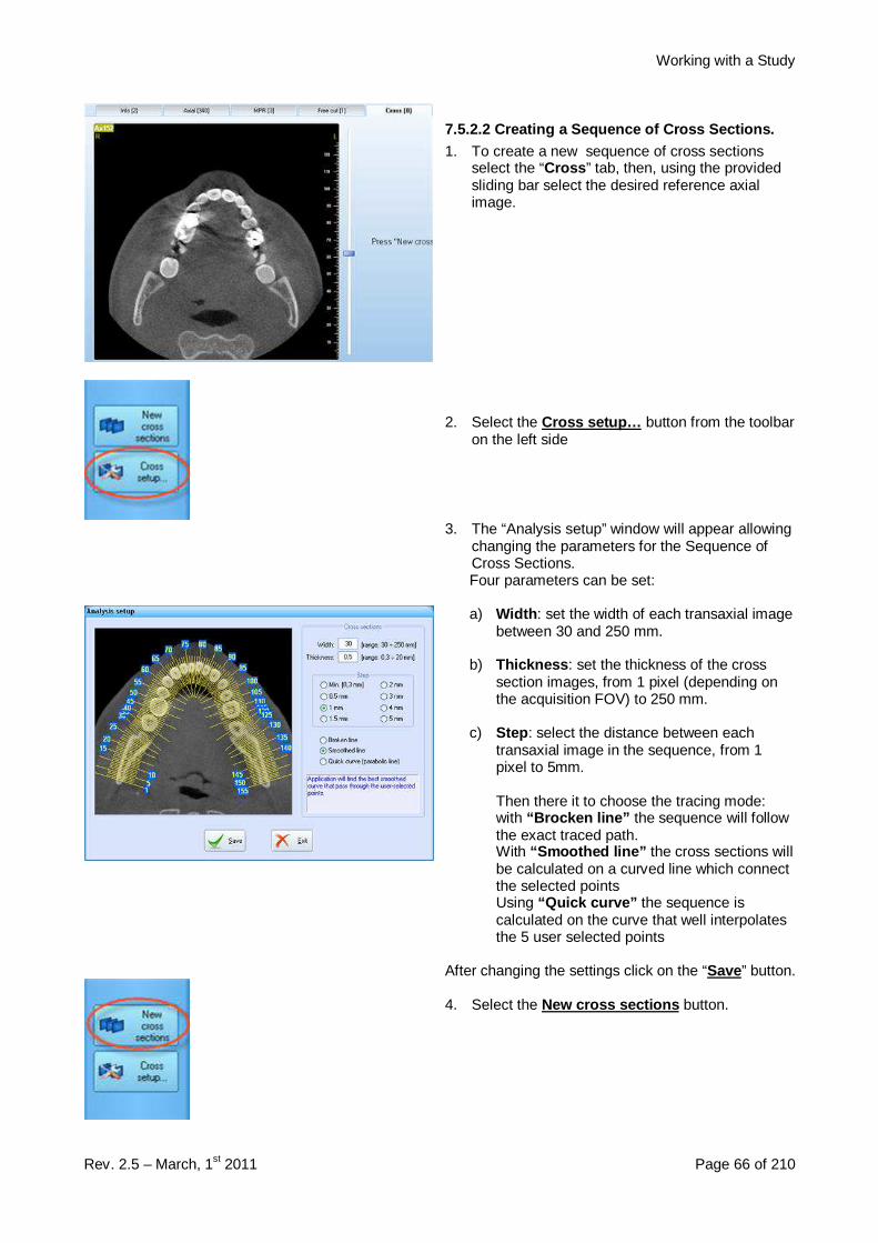
Working with a Study
Rev. 2.5 – March, 1st 2011 Page 66 of 210
7.5.2.2 Creating a Sequence of Cross Sections.1. To create a new sequence of cross sections
select the “Cross ” tab, then, using the providedsliding bar select the desired reference axialimage.
2. Select the Cross setup… button from the toolbaron the left side
3. The “Analysis setup” window will appear allowingchanging the parameters for the Sequence ofCross Sections.Four parameters can be set:
a) Width : set the width of each transaxial imagebetween 30 and 250 mm.
b) Thickness : set the thickness of the crosssection images, from 1 pixel (depending onthe acquisition FOV) to 250 mm.
c) Step : select the distance between eachtransaxial image in the sequence, from 1pixel to 5mm.
Then there it to choose the tracing mode:with “Brocken line” the sequence will followthe exact traced path.With “Smoothed line” the cross sections willbe calculated on a curved line which connectthe selected pointsUsing “Quick curve” the sequence iscalculated on the curve that well interpolatesthe 5 user selected points
After changing the settings click on the “Save” button.
4. Select the New cross sections button.

Working with a Study
Rev. 2.5 – March, 1st 2011 Page 67 of 210
5. The cursor will change to reflect the selectedcommand.
6. Left click inside the axial image, to define the firstpoint of the path of the sequence.
7. Drag the line and left click where you wish tobend your arch. Using the mouse wheel it ispossible to navigate through the axial imageswhile tracing the arch.
8. Right click to set the end point of the path.
9. The new image will appear beside the axial sliceused as reference image.
Clicking on the axial image the correspondingcross section will be highlighted.

Working with a Study
Rev. 2.5 – March, 1st 2011 Page 68 of 210
7.5.3 Panoramic Sections
7.5.3.1 What is a Panoramic section?Panoramics are images perpendicular to the axialplane.
The height of the images is the same as the height ofthe volume.
The thickness and distance between each image canvary.
7.5.3.2 Creating a Panoramic Section.1. To create a new panoramic select the “Panorex ”
tab, then, using the provided sliding bar selectthe desired reference axial image.
2. Select the Panorex Setup… button ftom thetoolbar on the left.
3. The “Analysis setup” window will appear allowingchanging the parameters for the Panoramicsections.Three parameters can be set:
a) Number of panoramics : number ofpanoramics created by the software; one canchoose between:• Single (maximum thickness = 50mm)• Multiple, selecting an odd number
between 3 and 31 (maximum thickness =15 mm);

Working with a Study
Rev. 2.5 – March, 1st 2011 Page 69 of 210
b) Thickness : set the thickness of the imagesbetween the size of a Voxel and themaximum allowed.
c) Distance : set the distance between eachimage between the size of a Voxel and 10mm.
d) Show pano thick highlights the panoramicthisckenss.
e) Draw middle line (available only if the Showpano thick button is enabled) drawn thecentral reference of the panoramic.
f) Then there it to choose the tracing mode:with “Brocken line” the panoramic will followthe exact traced path.With “Smoothed line” the panoramic sectionwill be calculated on a curved line whichconnect the selected pointsUsing “Quick curve” the panoramic iscalculated on the curve that well interpolatesthe 5 user selected points
After changing the settings click on the “Save” button.
4. Select the New panorex section(s) button.
5. The cursor will change to reflect the selectedcommand.Left click inside the axial image, to define thefirst point of the path of the panoramic section.
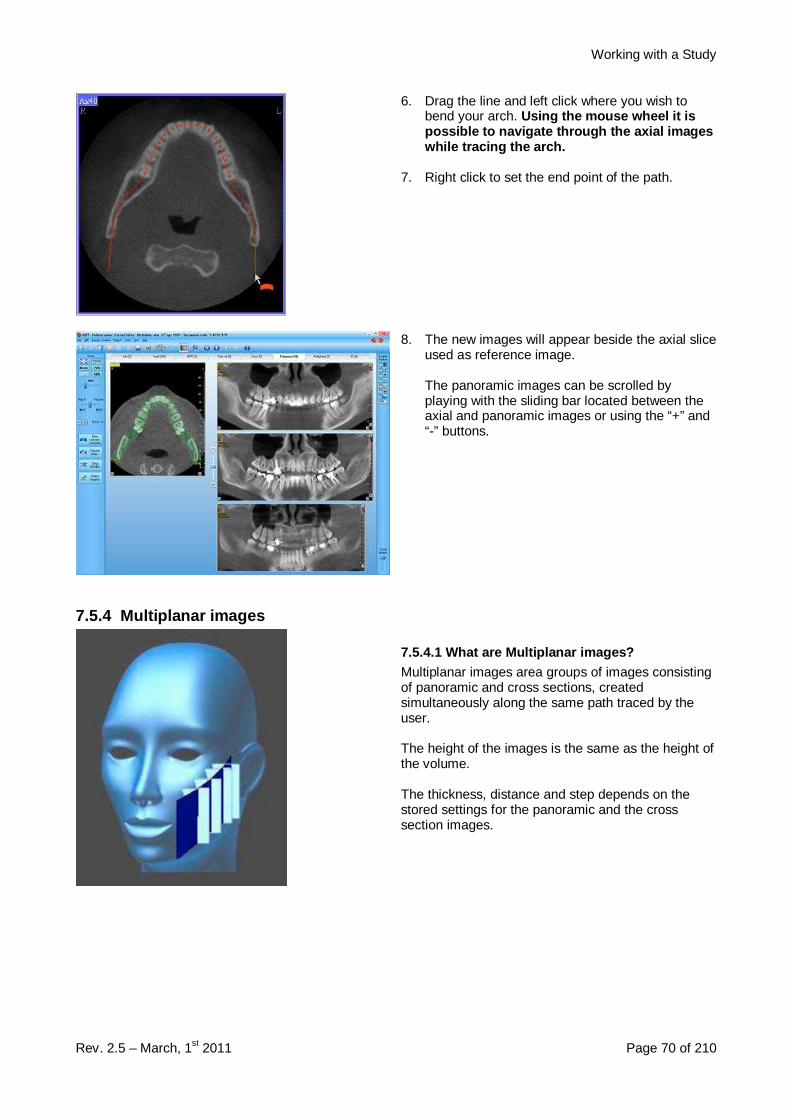
Working with a Study
Rev. 2.5 – March, 1st 2011 Page 70 of 210
6. Drag the line and left click where you wish tobend your arch. Using the mouse wheel it ispossible to navigate through the axial imageswhile tracing the arch.
7. Right click to set the end point of the path.
8. The new images will appear beside the axial sliceused as reference image.
The panoramic images can be scrolled byplaying with the sliding bar located between theaxial and panoramic images or using the “+” and“-” buttons.
7.5.4 Multiplanar images
7.5.4.1 What are Multiplanar images?Multiplanar images area groups of images consistingof panoramic and cross sections, createdsimultaneously along the same path traced by theuser.
The height of the images is the same as the height ofthe volume.
The thickness, distance and step depends on thestored settings for the panoramic and the crosssection images.

Working with a Study
Rev. 2.5 – March, 1st 2011 Page 71 of 210
7.5.4.2 Creating Multiplanar images.1. To create a new panoramic select the
“Multiplanar ” tab, then, using the providedsliding bar select the desired reference axialimage.
2. From the left bar select the Cross + Panorexsetup… button
In this case the “Analysis setup” window containsboth the cross parameters and the panoramic ones(see paragraph 7.5.2.2 and 7.5.3.2)
3. Select the New multiplanar section button.

Working with a Study
Rev. 2.5 – March, 1st 2011 Page 72 of 210
4. The cursor will change to reflect the selectedcommand.Left click inside the axial image, to define the firstpoint of the path of the panoramic section.
5. Drag the line and left click where you wish tobend your arch. Using the mouse wheel it ispossible to navigate through the axial imageswhile tracing the arch.
6. Right click to set the end point of the path.
7. The new images will appear beside the axial sliceused as reference image.
Depending on the visualization status of eachsingle cross section, the reference line drawn onthe axial image could be:
• Continue if the cross section is completelyshown.
• Dashed if the cross section is partially shown
• Hide if the cross section is not shown.
Vertical reference lines are drawn, using the samecriteria of the axials, on the panoramic image torepresent where the cross sections are located.These lines can be hide unchecking the optionslocated under the View → Show/Hide crossreference on panoramic menu.
For additional information about the panoramicimages please refer to chapter 0 “Panoramic Sections”.
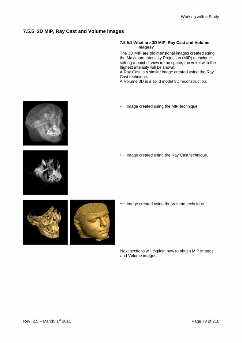
Working with a Study
Rev. 2.5 – March, 1st 2011 Page 73 of 210
7.5.5 3D MIP, Ray Cast and Volume images
7.5.5.1 What are 3D MIP, Ray Cast and Volumeimages?
The 3D MIP are tridimensional images created usingthe Maximum Intenstity Projection (MIP) technique:setting a point of view in the space, the voxel with thehighest intensity will be shown.A Ray Cast is a similar image created using the RayCast technique.A Volume 3D is a solid model 3D reconstruction.
← Image created using the MIP technique.
← Image created using the Ray Cast technique.
← Image created using the Volume technique.
Next sections will explain how to obtain MIP imagesand Volume images.

Working with a Study
Rev. 2.5 – March, 1st 2011 Page 74 of 210
7.5.5.2 Creating 3D MIP, Ray Cast and solid (RayCast + shadow) images.
1. To create a new panoramic select the “3D” tab,then, using the provided sliding bar select thedesired reference axial image.
2. Select the New 3D model button from the toolbaron the left.
3. The 3D MIP/RayCast/Volume window will appear.Initially only three buttons are enabled: the“Load3D” and the 3D default settings buttons locatedon the top left corner and the “Exit” button,located on the bottom right corner. The first timethis window is used is necessary to load andelaborate the initial 3D model.
4. Before loading the model is possible to choose thetype of image you wish to create: MIP, Ray Cast ora solid reconstruction (Volume); in this examplethe default settings will be kept in order to showthe functionalities of this window.The “Surface smooth” flag applies a smooth filter inorder to remove irregularities or roughness fromthe image .The “Edge enhancer” option applies an edgeenhancer filter on the 3D model to improve thesharpness of the image, this function isrecommended in the RayCast reconstruction.
5. It is now possible to select the quality of thereconstructed model, using the ‘+’ and ‘-’ buttonsof the Model quality field. Increasing the quality willrequire longer processing time, so it is suggestedto start working with the default settings andchange the quality subsequently.
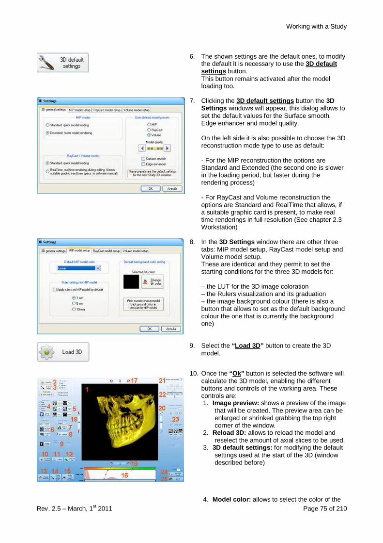
Working with a Study
Rev. 2.5 – March, 1st 2011 Page 75 of 210
6. The shown settings are the default ones, to modifythe default it is necessary to use the 3D defaultsettings button.This button remains activated after the modelloading too.
7. Clicking the 3D default settings button the 3DSettings windows will appear, this dialog allows toset the default values for the Surface smooth,Edge enhancer and model quality.
On the left side it is also possible to choose the 3Dreconstruction mode type to use as default:
- For the MIP reconstruction the options areStandard and Extended (the second one is slowerin the loading period, but faster during therendering process)
- For RayCast and Volume reconstruction theoptions are Standard and RealTime that allows, ifa suitable graphic card is present, to make realtime renderings in full resolution (See chapter 2.3Workstation)
8. In the 3D Settings window there are other threetabs: MIP model setup, RayCast model setup andVolume model setup.These are identical and they permit to set thestarting conditions for the three 3D models for:
– the LUT for the 3D image coloration– the Rulers visualization and its graduation– the image background colour (there is also abutton that allows to set as the default backgroundcolour the one that is currently the backgroundone)
9. Select the “Load 3D” button to create the 3Dmodel.
10. Once the “Ok” button is selected the software willcalculate the 3D model, enabling the differentbuttons and controls of the working area. Thesecontrols are:1. Image preview: shows a preview of the image
that will be created. The preview area can beenlarged or shrinked grabbing the top rightcorner of the window.
2. Reload 3D: allows to reload the model andreselect the amount of axial slices to be used.
3. 3D default settings: for modifying the defaultsettings used at the start of the 3D (windowdescribed before)
4. Model color: allows to select the color of the
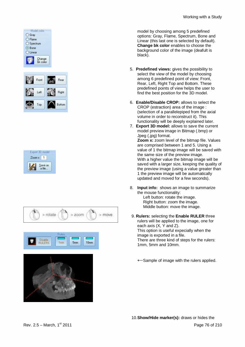
Working with a Study
Rev. 2.5 – March, 1st 2011 Page 76 of 210
model by choosing among 5 predefinedoptions: Gray, Flame, Spectrum, Bone andLinear (this last one is selected by default).Change bk color enables to choose thebackground color of the image (deafult isblack).
5. Predefined views: gives the possibility toselect the view of the model by choosingamong 6 predefined point of view: Front,Rear, Left, Right Top and Bottom. Thesepredefined points of view helps the user tofind the best position for the 3D model.
6. Enable/Disable CROP: allows to select theCROP (estraction) area of the image :(selection of a parallelepiped from the axialvolume in order to reconstruct it). Thisfunctionality will be deeply explained later.
7. Export 3D model: allows to save the currentmodel preview image in Bitmap (.bmp) orJpeg (.jpg) format.Zoom x: zoom level of the bitmap file. Valuesare comprised between 1 and 5. Using avalue of 1 the bitmap image will be saved withthe same size of the preview image.With a higher value the bitmap image will besaved with a larger size, keeping the quality ofthe preview image (using a value greater than1 the preview image will be automaticallyupdated and moved for a few seconds).
8. Input info: shows an image to summarizethe mouse functionality:
Left button: rotate the image.Right button: zoom the image.Middle button: move the image.
9. Rulers: selecting the Enable RULER threerulers will be applied to the image, one foreach axis (X, Y and Z).This option is useful expecially when theimage is exported in a file.There are three kind of steps for the rulers:1mm, 5mm and 10mm.
←Sample of image with the rulers applied.
10. Show/Hide marker(s): draws or hides the
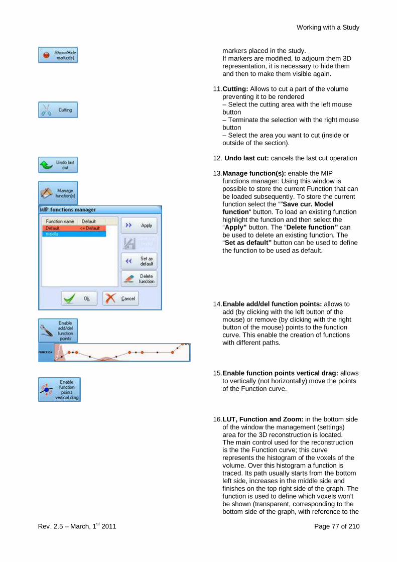
Working with a Study
Rev. 2.5 – March, 1st 2011 Page 77 of 210
markers placed in the study.If markers are modified, to adjourn them 3Drepresentation, it is necessary to hide themand then to make them visible again.
11. Cutting: Allows to cut a part of the volumepreventing it to be rendered– Select the cutting area with the left mousebutton– Terminate the selection with the right mousebutton– Select the area you want to cut (inside oroutside of the section).
12. Undo last cut: cancels the last cut operation
13. Manage function(s): enable the MIPfunctions manager: Using this window ispossible to store the current Function that canbe loaded subsequently. To store the currentfunction select the “”Save cur. Modelfunction “ button. To load an existing functionhighlight the function and then select the“Apply” button. The “Delete function” canbe used to delete an existing function. The“Set as default” button can be used to definethe function to be used as default.
14. Enable add/del function points: allows toadd (by clicking with the left button of themouse) or remove (by clicking with the rightbutton of the mouse) points to the functioncurve. This enable the creation of functionswith different paths.
15. Enable function points vertical drag: allowsto vertically (not horizontally) move the pointsof the Function curve.
16. LUT, Function and Zoom: in the bottom sideof the window the management (settings)area for the 3D reconstruction is located.The main control used for the reconstructionis the the Function curve; this curverepresents the histogram of the voxels of thevolume. Over this histogram a function istraced. Its path usually starts from the bottomleft side, increases in the middle side andfinishes on the top right side of the graph. Thefunction is used to define which voxels won’tbe shown (transparent, corresponding to thebottom side of the graph, with reference to the
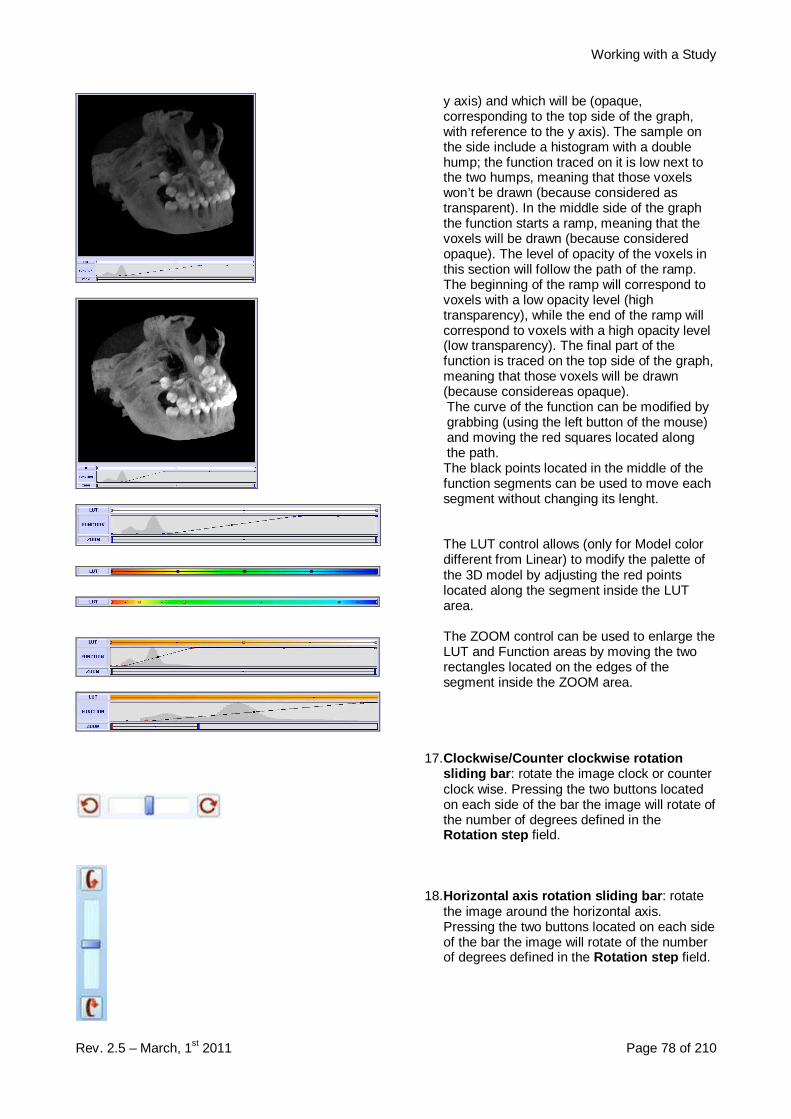
Working with a Study
Rev. 2.5 – March, 1st 2011 Page 78 of 210
y axis) and which will be (opaque,corresponding to the top side of the graph,with reference to the y axis). The sample onthe side include a histogram with a doublehump; the function traced on it is low next tothe two humps, meaning that those voxelswon’t be drawn (because considered astransparent). In the middle side of the graphthe function starts a ramp, meaning that thevoxels will be drawn (because consideredopaque). The level of opacity of the voxels inthis section will follow the path of the ramp.The beginning of the ramp will correspond tovoxels with a low opacity level (hightransparency), while the end of the ramp willcorrespond to voxels with a high opacity level(low transparency). The final part of thefunction is traced on the top side of the graph,meaning that those voxels will be drawn(because considereas opaque).The curve of the function can be modified bygrabbing (using the left button of the mouse)and moving the red squares located alongthe path.The black points located in the middle of thefunction segments can be used to move eachsegment without changing its lenght.
The LUT control allows (only for Model colordifferent from Linear) to modify the palette ofthe 3D model by adjusting the red pointslocated along the segment inside the LUTarea.
The ZOOM control can be used to enlarge theLUT and Function areas by moving the tworectangles located on the edges of thesegment inside the ZOOM area.
17. Clockwise/Counter clockwise rotationsliding bar : rotate the image clock or counterclock wise. Pressing the two buttons locatedon each side of the bar the image will rotate ofthe number of degrees defined in theRotation step field.
18. Horizontal axis rotation sliding bar : rotatethe image around the horizontal axis.Pressing the two buttons located on each sideof the bar the image will rotate of the numberof degrees defined in the Rotation step field.

Working with a Study
Rev. 2.5 – March, 1st 2011 Page 79 of 210
19. Vertical axis rotation sliding bar : rotate theimage around the vertical axis. Pressing thetwo buttons located on each side of the barthe image will rotate of the number of degreesdefined in the Rotation step field.
20. Zoom sliding bar : increase/decrease themagnification of the image
21. Rotation step : define the number of degreeof which the image will rotate when therotation sliding bar buttons are pressed.
22. Slider rotation speed : set the image’srotational slider sensibility.Only the correct slider is active.
23. Model axis adjustment: permette diaggiustare l’orientamento di default delmodello. Allows to adjust the axis modelorientation. This functionality will be deeplyexplained later
24. Add image to study: add the image of thepreview area, magnified by a factor defined bythe Zoom x field, to the study under the 3Dimages section.Higher will be the zoom value higher will bethe resolution of the printed image.
25. Exit: close the window and return to thestudy. Besides the window is closed it is stillactive, meaning that next time it will be open itwill keep the last settings avoiding to reloadthe model.
11. Selecting the “Enable CROP” button, the “SetCROP (X, Y)” and “Set CROP (Z) ” buttonsbecame available.
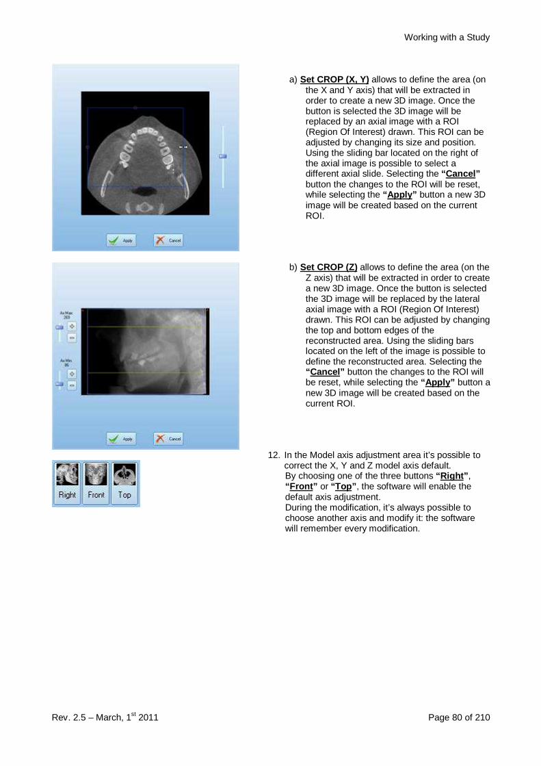
Working with a Study
Rev. 2.5 – March, 1st 2011 Page 80 of 210
a) Set CROP (X, Y) allows to define the area (onthe X and Y axis) that will be extracted inorder to create a new 3D image. Once thebutton is selected the 3D image will bereplaced by an axial image with a ROI(Region Of Interest) drawn. This ROI can beadjusted by changing its size and position.Using the sliding bar located on the right ofthe axial image is possible to select adifferent axial slide. Selecting the “Cancel”button the changes to the ROI will be reset,while selecting the “Apply” button a new 3Dimage will be created based on the currentROI.
b) Set CROP (Z) allows to define the area (on theZ axis) that will be extracted in order to createa new 3D image. Once the button is selectedthe 3D image will be replaced by the lateralaxial image with a ROI (Region Of Interest)drawn. This ROI can be adjusted by changingthe top and bottom edges of thereconstructed area. Using the sliding barslocated on the left of the image is possible todefine the reconstructed area. Selecting the“Cancel” button the changes to the ROI willbe reset, while selecting the “Apply” button anew 3D image will be created based on thecurrent ROI.
12. In the Model axis adjustment area it’s possible tocorrect the X, Y and Z model axis default.By choosing one of the three buttons “Right” ,“Front” or “Top ” , the software will enable thedefault axis adjustment.During the modification, it’s always possible tochoose another axis and modify it: the softwarewill remember every modification.
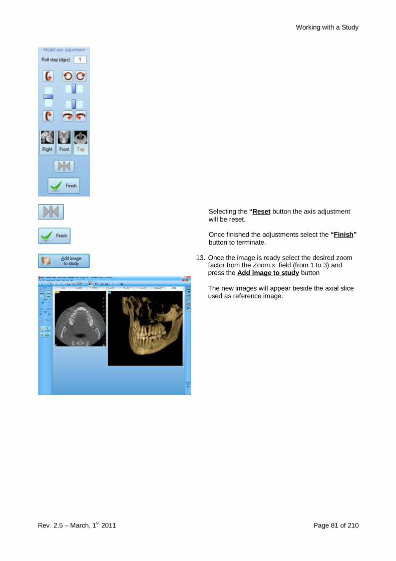
Working with a Study
Rev. 2.5 – March, 1st 2011 Page 81 of 210
Selecting the “Reset button the axis adjustmentwill be reset.
Once finished the adjustments select the “Finish”button to terminate.
13. Once the image is ready select the desired zoomfactor from the Zoom x field (from 1 to 3) andpress the Add image to study button
The new images will appear beside the axial sliceused as reference image.
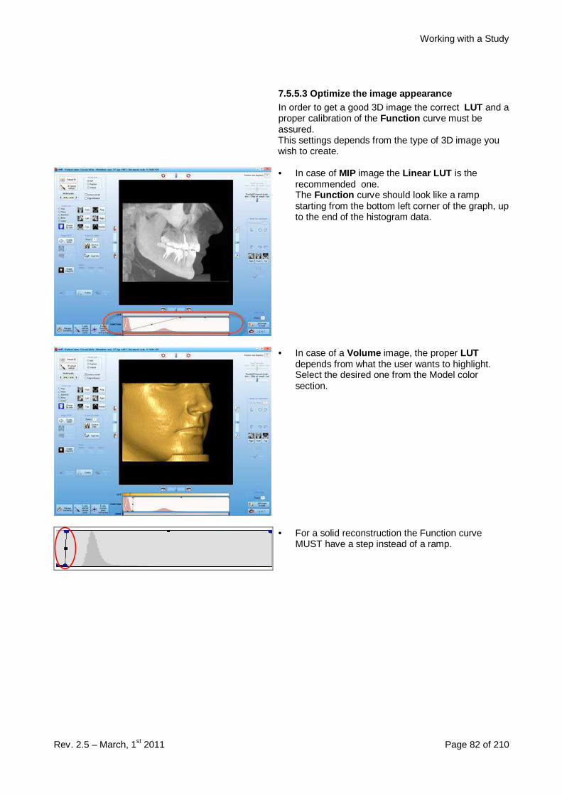
Working with a Study
Rev. 2.5 – March, 1st 2011 Page 82 of 210
7.5.5.3 Optimize the image appearanceIn order to get a good 3D image the correct LUT and aproper calibration of the Function curve must beassured.This settings depends from the type of 3D image youwish to create.
• In case of MIP image the Linear LUT is therecommended one.The Function curve should look like a rampstarting from the bottom left corner of the graph, upto the end of the histogram data.
• In case of a Volume image, the proper LUTdepends from what the user wants to highlight.Select the desired one from the Model colorsection.
• For a solid reconstruction the Function curveMUST have a step instead of a ramp.

Working with a Study
Rev. 2.5 – March, 1st 2011 Page 83 of 210
• Adjust the Function curve to select the tissue(bone or soft) you wish to display.
← Image with bone tissue highlighted.
← Image with soft tissue highlighted.

Working with a Study
Rev. 2.5 – March, 1st 2011 Page 84 of 210
7.5.6 Dynamic 3D images
7.5.6.1 What is a dynamic 3D image?The dynamic 3D images are images similar to the onesdescribed in the previous chapter, created with adifferent method.The dynamic 3D images include additional settingsand features like the possibility to apply differentcolors, transparency levels, zoom levels etc...
For each image the height, width and deep can bechanged.
7.5.6.2 Creating a dynamic 3D image.The menu for the dynamic 3D image is alwaysenabled, also if other images are currently showed onthe screen.
1. From the menu selectImages creation ���� New dynamic 3D
2. A window showing a black image will appear.Initially only two buttons are enabled: the“Loadimage” button located on the top left corner andthe “Exit” button, located on the bottom rightcorner.The first time the dynamic 3D window is used isnecessary to load and elaborate the initial 3Dmodel.For this purpose select the “Load image” button.
3. The software will create the initial 3D model andwill enabled the different controls of the window.These controls include:
1. Preview area: show a preview of the imagethat will be created.
2. Reload Img: allow to reload the model andselect the amount of axial to be used for itscreation.
3. Reset image: reset all the applied settingsand retry to the initial 3D model.
4. Image quality: Allows to select the imagequality of the 3D model: Very high , High ,Mean and Low . The image quality affects thecalculation times, so higher quality will meanlonger times. It is suggested to use a lowquality during the 3D model adjustements andmove to a higher quality right before insertingthe image in the study. If the amount of axialimage is higher than 150, the Very highoption will be disable.

Working with a Study
Rev. 2.5 – March, 1st 2011 Page 85 of 210
The Smooth flag applies a smooth filter to theimage.
5. Enable/Disable CROP: allows to select theCROP (estraction) area of the image :(selection of a parallelepiped from the axialvolume in order to reconstruct it). Thisfunctionality will be deeply explained later.
6. Bone level: Using this sliding bar it ispossible to select the level of the tissue thatwill be shown; to visualize only the teeth usehigh levels, for the teeth and the skull useintermediate values while for the soft tissuelow values are suggested.
7. Opacity: Using this sliding bar it is possible toapply a transparency to the image thatincrease reducing the selected value. Thetransparency allows to view the internal areasof the skull.
8. Export 3D model: allows to save the currentmodel preview image in Bitmap (.bmp) orJpeg (.jpg) format.Zoom x: zoom level of the bitmap file. Valuesare comprised between 1 and 5. Using avalue of 1 the bitmap image will be saved withthe same size of the preview image.With a higher value the bitmap image will besaved with a larger size, keeping the quality ofthe preview image (using a value greater than1 the preview image will be automaticallyupdated and moved for a few seconds).For values of Zoom higher than 1 only theBMP storage format (not JPEG) will beavailable.
9. Input info: show a image to summarize themouse functionality.Left button: rotate the image.Right button: zoom the image.Middle button: Move the image.
10. Input type: switch between two differentfunctionality for the rotation, zoom andmovements of the image:Manual: After one of the mouse buttons ispressed the mouse must be move manually inorder to apply the desired changes.Automatic: After one of the mouse buttons ispressed the associated action (rotation, zoomand movement) is automatically started by thesoftware until the button is released.
11. Change bk color: allows to change thebackground color (usually black).
12. Color specular: allows to apply a lightreflection effect to the image.
13. Color diffuse: allows to change thebrightness of the color.
14. Enable/Disable cut planes: allows to applyto the 3D model three different planes (X, Y eZ). Once the planes are enabled they can bemoved by adjusting the corresponding slidingbars.The Enable cut X , Enable cut Y and Enablecut Z buttons enable/disable the single
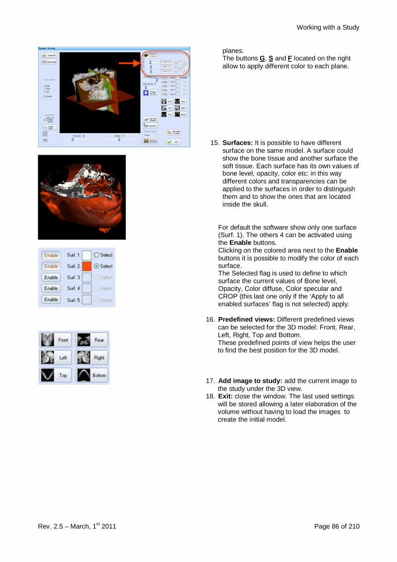
Working with a Study
Rev. 2.5 – March, 1st 2011 Page 86 of 210
planes.The buttons G, S and F located on the rightallow to apply different color to each plane.
15. Surfaces: It is possible to have differentsurface on the same model. A surface couldshow the bone tissue and another surface thesoft tissue. Each surface has its own values ofbone level, opacity, color etc: in this waydifferent colors and transparencies can beapplied to the surfaces in order to distinguishthem and to show the ones that are locatedinside the skull.
For default the software show only one surface(Surf. 1). The others 4 can be activated usingthe Enable buttons.Clicking on the colored area next to the Enablebuttons it is possible to modify the color of eachsurface.The Selected flag is used to define to whichsurface the current values of Bone level,Opacity, Color diffuse, Color specular andCROP (this last one only if the ‘Apply to allenabled surfaces’ flag is not selected) apply.
16. Predefined views: Different predefined viewscan be selected for the 3D model: Front, Rear,Left, Right, Top and Bottom.These predefined points of view helps the userto find the best position for the 3D model.
17. Add image to study: add the current image tothe study under the 3D view.
18. Exit: close the window. The last used settingswill be stored allowing a later elaboration of thevolume without having to load the images tocreate the initial model.

Working with a Study
Rev. 2.5 – March, 1st 2011 Page 87 of 210
7. Selecting the “Enable CROP” button, the “SetCROP (X, Y)” and “Set CROP (Z) ” buttonsbecame available.
a) Set CROP (X, Y) allows to define the area (on theX and Y axis) that will be extracted in order tocreate a new 3D image. Once the button isselected the 3D image will be replaced by an axialimage with a ROI (Region Of Interest) drawn. ThisROI can be adjusted by changing its size andposition. Using the sliding bar located on the rightof the axial image is possible to select a differentaxial slide. Selecting the “Cancel” button thechanges to the ROI will be reset, while selectingthe “Apply” button a new 3D image will becreated based on the current ROI.
b) Set CROP (Z) allows to define the area (on the Zaxis) that will be extracted in order to create a new3D image. Once the button is selected the 3Dimage will be replaced by the lateral axial imagewith a ROI (Region Of Interest) drawn. This ROIcan be adjusted by changing the top and bottomedges of the reconstructed area. Using the slidingbars located on the left of the image is possible todefine the reconstructed area. Selecting the“Cancel” button the changes to the ROI will bereset, while selecting the “Apply” button a new 3Dimage will be created based on the current ROI.
Using the ‘Apply to all enabled surfaces ’ it ispossible to apply the CROP to all the selectedsurfaces (the ones with the ‘Enable ’ buttonselected) or only to the currente selected.
8. Once the image has been created, select the “Addimage to study” to insert it in the study.

Working with a Study
Rev. 2.5 – March, 1st 2011 Page 88 of 210
9. The new 3D image will appear beside the axialreference image. This axial is the one currentlyshown on the axial view. If three axial images arecurrently shown, the central one will be visualized.
7.6 Deleting existing images.The only images that can be deleted are Single Cross sections (Free cut ), sequence of cross sections(Cross ), panoramic (Panorex ), Multiplanar and 3D. Lateral view, axial images and MPR images cannot bedeleted, since they represent the base of the study.
1. Select the Tab which represents the image typeto delete.
2. From the toolbar on the left, select the “DeleteImage(s) ” button.
3. The cursor will change to reflect the selectedcommand. Left click inside the image(s) you wantto delete.
4. Right click to terminate the command.
7.6.1 Deleting single cross sections from a sequen ce of cross sectionsIt is possible to delete one or more single sections, belonging to a sequence of cross sections.
1. From the “Image creation tools” toolbar, selectthe “Delete Single Image ” button.
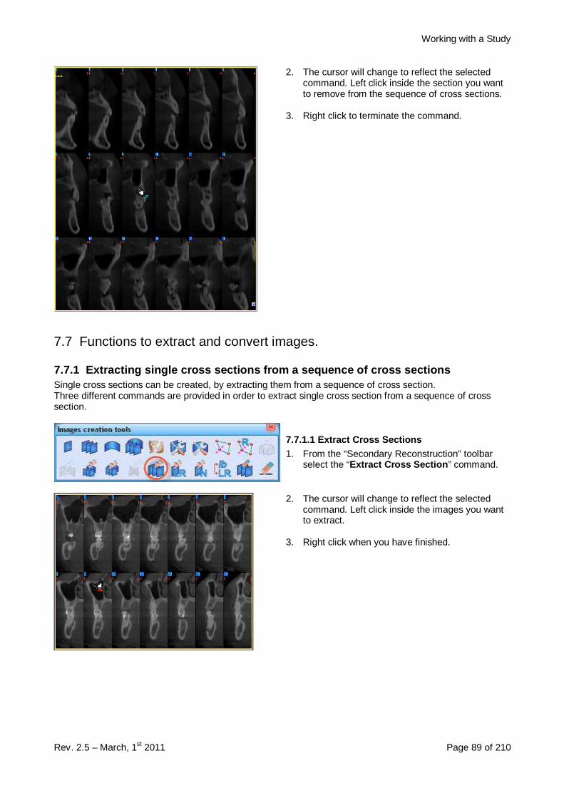
Working with a Study
Rev. 2.5 – March, 1st 2011 Page 89 of 210
2. The cursor will change to reflect the selectedcommand. Left click inside the section you wantto remove from the sequence of cross sections.
3. Right click to terminate the command.
7.7 Functions to extract and convert images.
7.7.1 Extracting single cross sections from a sequ ence of cross sectionsSingle cross sections can be created, by extracting them from a sequence of cross section.Three different commands are provided in order to extract single cross section from a sequence of crosssection.
7.7.1.1 Extract Cross Sections1. From the “Secondary Reconstruction” toolbar
select the “Extract Cross Section ” command.
2. The cursor will change to reflect the selectedcommand. Left click inside the images you wantto extract.
3. Right click when you have finished.
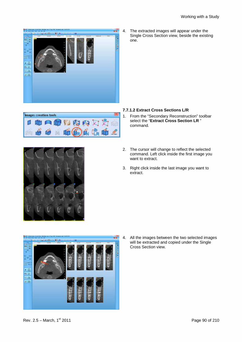
Working with a Study
Rev. 2.5 – March, 1st 2011 Page 90 of 210
4. The extracted images will appear under theSingle Cross Section view, beside the existingone.
7.7.1.2 Extract Cross Sections L/R1. From the “Secondary Reconstruction” toolbar
select the “Extract Cross Section LR ”command.
2. The cursor will change to reflect the selectedcommand. Left click inside the first image youwant to extract.
3. Right click inside the last image you want toextract.
4. All the images between the two selected imageswill be extracted and copied under the SingleCross Section view.
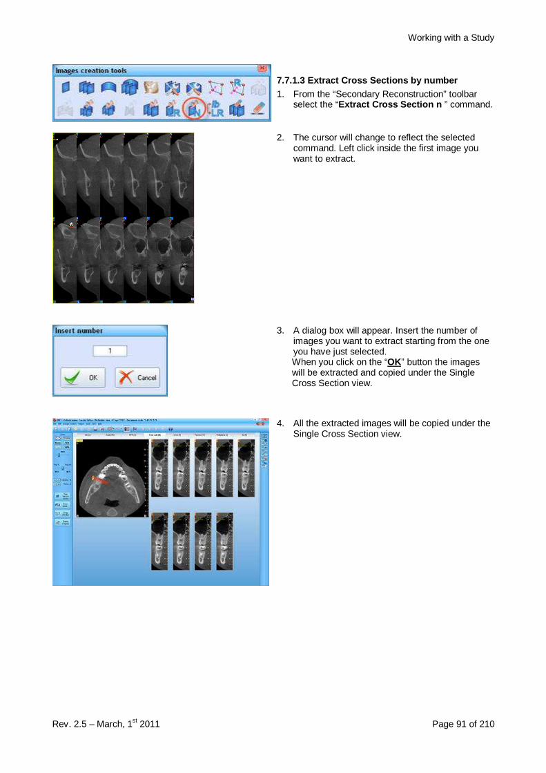
Working with a Study
Rev. 2.5 – March, 1st 2011 Page 91 of 210
7.7.1.3 Extract Cross Sections by number1. From the “Secondary Reconstruction” toolbar
select the “Extract Cross Section n ” command.
2. The cursor will change to reflect the selectedcommand. Left click inside the first image youwant to extract.
3. A dialog box will appear. Insert the number ofimages you want to extract starting from the oneyou have just selected.When you click on the “OK” button the imageswill be extracted and copied under the SingleCross Section view.
4. All the extracted images will be copied under theSingle Cross Section view.
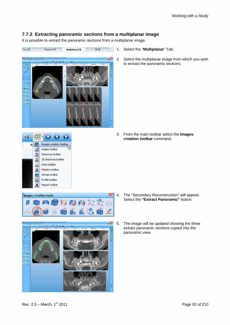
Working with a Study
Rev. 2.5 – March, 1st 2011 Page 92 of 210
7.7.2 Extracting panoramic sections from a multipl anar imageIt is possible to extract the panoramic sections from a multiplanar image.
1. Select the “Multiplanar ” Tab.
2. Select the multiplanar image from which you wishto extract the panoramic sections.
3. From the main toolbar select the Imagescreation toolbar command.
4. The “Secondary Reconstruction” will appear.Select the “Extract Panoramic” button.
5. The image will be updated showing the threeextract panoramic sections copied into thepanoramic view.

Working with a Study
Rev. 2.5 – March, 1st 2011 Page 93 of 210
7.7.3 Extracting sequence of cross sections from a multiplanar imageIt is possible to extract sequence of cross sections from a multiplanar image.
1. Select the “Multiplanar ” Tab.
2. Select the multiplanar image from which you wishto extract the panoramic sections.
3. From the main toolbar select the Imagescreation toolbar command.
4. The “Secondary Reconstruction” will appear.Select the “ Extract sequence ” button.
5. The image will be updated showing the extractedsequence of cross sections.

Working with a Study
Rev. 2.5 – March, 1st 2011 Page 94 of 210
7.7.4 Extracting Coronal and Sagittal sections fro m the MPR view1. Select the “MPR” Tab.
2. The MPR view will appear. For a completeexplanation of this view please refere to chapter6.4 “MPR view“.
3. From the main toolbar select “Images creationtoolbar ” button.
4. The “Secondary Reconstruction” will appear.Select the “ Extract coronal/sagittal” button.
5. The cursor will change to reflect the selectedcommand. Click on the image (coronal orsagittal) you wish to extract.
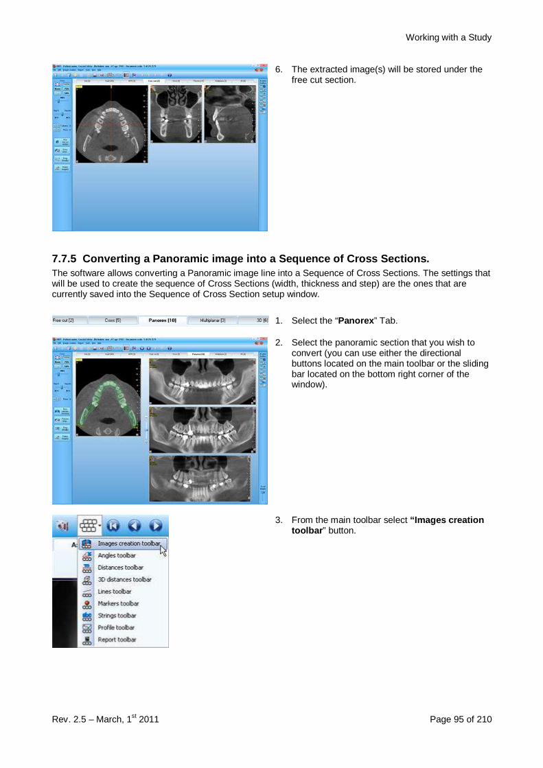
Working with a Study
Rev. 2.5 – March, 1st 2011 Page 95 of 210
6. The extracted image(s) will be stored under thefree cut section.
7.7.5 Converting a Panoramic image into a Sequence of Cross Sections.The software allows converting a Panoramic image line into a Sequence of Cross Sections. The settings thatwill be used to create the sequence of Cross Sections (width, thickness and step) are the ones that arecurrently saved into the Sequence of Cross Section setup window.
1. Select the “Panorex ” Tab.
2. Select the panoramic section that you wish toconvert (you can use either the directionalbuttons located on the main toolbar or the slidingbar located on the bottom right corner of thewindow).
3. From the main toolbar select “Images creationtoolbar ” button.

Working with a Study
Rev. 2.5 – March, 1st 2011 Page 96 of 210
4. The “Secondary Reconstruction” toolbar willappear. Select the “Panorex -> Crosses ” button.
5. The new Sequence of Cross Sections will bedisplayed.
7.7.6 Converting a Sequence of Cross Sections into a Panoramic image.Another possibility is to convert a Sequence of Cross Sections into Panoramic images. The settings that willbe used to create the Panoramic images (thickness and distance) are the ones that are currently saved intothe Panoramic setup window.
1. Select the “Cross ” Tab.
2. Select the Sequence of Cross Sections that youwish to convert (you can use either thedirectional buttons located on the main toolbar orthe sliding bar located on the bottom right cornerof the window).
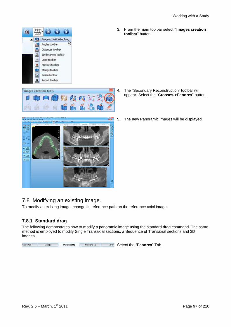
Working with a Study
Rev. 2.5 – March, 1st 2011 Page 97 of 210
3. From the main toolbar select “Images creationtoolbar ” button.
4. The “Secondary Reconstruction” toolbar willappear. Select the “Crosses->Panorex ” button.
5. The new Panoramic images will be displayed.
7.8 Modifying an existing image.To modify an existing image, change its reference path on the reference axial image.
7.8.1 Standard dragThe following demonstrates how to modify a panoramic image using the standard drag command. The samemethod is employed to modify Single Transaxial sections, a Sequence of Transaxial sections and 3Dimages.
Select the “Panorex ” Tab.

Working with a Study
Rev. 2.5 – March, 1st 2011 Page 98 of 210
Select the panoramic section you want to modify (youcan use either the directional buttons located on themain toolbar or the sliding bar located on the bottomright corner of the window).
Click on the “Drag ” button located on the “ Imagescreation tools”.
The reference path on the axial image will behighlighted along with red targets used to drag thepath for image modification.
Left click in the targets and drag the target with theleft button depressed. Release the button when thetarget is in the desired location.Clicking between to red targets is possible to movethe entire curve
Clicking on the yellow targets in the middle it ispossible to stretch the curve.Clicking on the yellow targets in the corners it ispossible to rotate the curve
Pressing the CTRL key and moving the mouse wheelit is possible to enlarge/reduce the curve.
Using the mouse wheel it is possible to navigatethrough the axial images while dragging the arch(not available for drag of single cross and 3D).
To terminate the command right click.
A message will appear.
Click on the “Modify Current Image ” button tomodify the existing panoramic image.
Click on the “Create New Image ” button to create anew image without modifying the existing image.
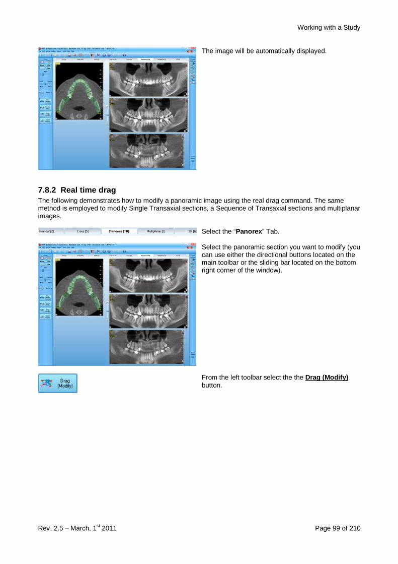
Working with a Study
Rev. 2.5 – March, 1st 2011 Page 99 of 210
The image will be automatically displayed.
7.8.2 Real time dragThe following demonstrates how to modify a panoramic image using the real drag command. The samemethod is employed to modify Single Transaxial sections, a Sequence of Transaxial sections and multiplanarimages.
Select the “Panorex ” Tab.
Select the panoramic section you want to modify (youcan use either the directional buttons located on themain toolbar or the sliding bar located on the bottomright corner of the window).
From the left toolbar select the the Drag (Modify)button.
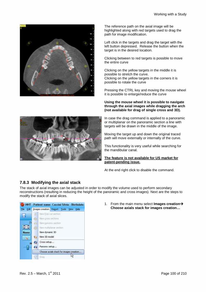
Working with a Study
Rev. 2.5 – March, 1st 2011 Page 100 of 210
The reference path on the axial image will behighlighted along with red targets used to drag thepath for image modification.
Left click in the targets and drag the target with theleft button depressed. Release the button when thetarget is in the desired location.
Clicking between to red targets is possible to movethe entire curve
Clicking on the yellow targets in the middle it ispossible to stretch the curve.Clicking on the yellow targets in the corners it ispossible to rotate the curve
Pressing the CTRL key and moving the mouse wheelit is possible to enlarge/reduce the curve
Using the mouse wheel it is possible to navigatethrough the axial images while dragging the arch(not available for drag of single cross and 3D).
In case the drag command is applied to a panoramicor multiplanar on the panoramic section a line withtargets will be drawn in the middle of the image.
Moving the target up and down the original tracedpath will move externally or internally of the curve.
This functionality is very useful while searching forthe mandibular canal.
The feature is not available for US market forpatent-pending issue.
At the end right click to disable the command.
7.8.3 Modifying the axial stackThe stack of axial images can be adjusted in order to modify the volume used to perform secondaryreconstructions (resulting in reducing the height of the panoramic and cross images). Next are the steps tomodify the stack of axial slices.
1. From the main menu select Images creation ����
Choose axials stack for images creation…
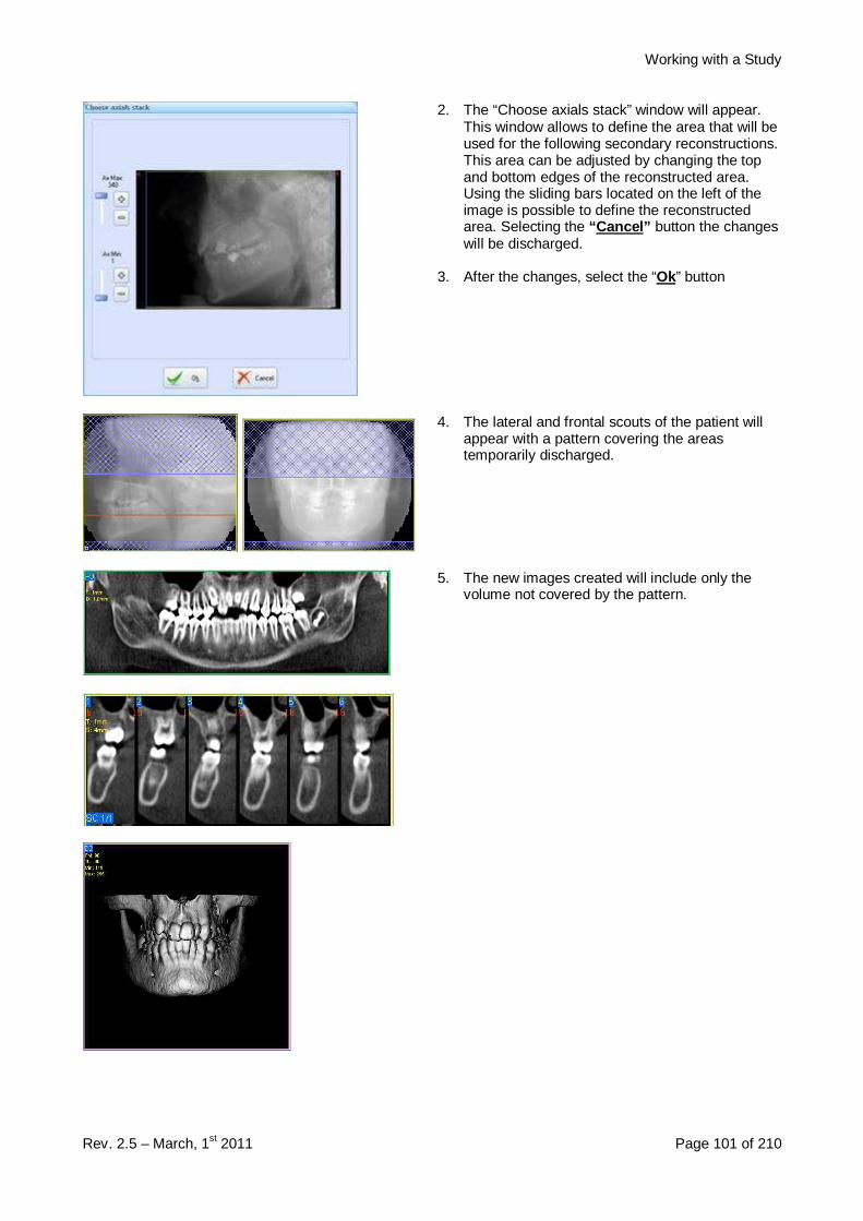
Working with a Study
Rev. 2.5 – March, 1st 2011 Page 101 of 210
2. The “Choose axials stack” window will appear.This window allows to define the area that will beused for the following secondary reconstructions.This area can be adjusted by changing the topand bottom edges of the reconstructed area.Using the sliding bars located on the left of theimage is possible to define the reconstructedarea. Selecting the “Cancel” button the changeswill be discharged.
3. After the changes, select the “Ok” button
4. The lateral and frontal scouts of the patient willappear with a pattern covering the areastemporarily discharged.
5. The new images created will include only thevolume not covered by the pattern.

Working with a Study
Rev. 2.5 – March, 1st 2011 Page 102 of 210
7.9 Moving among different images.Five buttons located on the main toolbar are available to switch among different types of images.
Info Tab: displays the scout images.
Axial Tab: displays the axial images.
MPR Tab: displays the MPR images.
Free cut Tab: displays the singlecross sections images.
Cross Tab: displays the seq. of crosssection view.
Panorex Tab: displays the panoramicimages.
Multiplanar Tab: displays themultiplanar images.
3D Tab: displays the 3D images.
To move between multiple images of the same type, use the four direction buttons. These buttons areenabled only if you have more than one image of the same type.
First image button: display the first image of the selected type.
Previous image button: display the previous image of the selected type.
Next image button: display the next image of the selected type.
Last image button: display the last image of the selected type.
7.10 Modifying image appearance.
7.10.1 Visualization windowThe visualization window allows selecting the tissues to display on the image depending on their density (itmodifies the relation between the 256 levels of gray that can be visualized and the values of the single pixelsof the image). It also allows adjusting the filter that can be applied to the images.
1. The “Visualization Window” can be open in twodifferent ways:
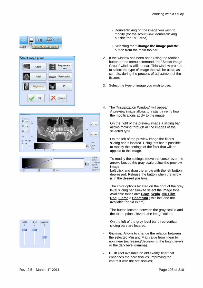
Working with a Study
Rev. 2.5 – March, 1st 2011 Page 103 of 210
• Doubleclicking on the image you wish tomodify (for the scout view, doubleclickingoutside the ROI area).
• Selecting the “Change the image palette ”button from the main toolbar.
2. If the window has been open using the toolbarbutton or the menu command, the “Select ImageGroup” window will appear. This window promptsto select the type of image that will be used, assample, during the process of adjustment of thetissues.
3. Select the type of image you wish to use.
4. The “Visualization Window” will appear.A preview image allows to instantly verify howthe modifications apply to the image.
On the right of the preview image a sliding barallows moving through all the images of theselected type.
On the left of the preview image the filter’ssliding bar is located. Using this bar is possibleto modify the settings of the filter that will beapplied to the image.
To modify the settings, move the cursor over thearrows beside the gray scale below the previewimage.Left click and drag the arrow with the left buttondepressed. Release the button when the arrowis in the desired position.
The color options located on the right of the graylevel sliding bar allow to select the image tone.Available tones are: Gray , Sepia, Blu Film ,Red, Flame e Spectrum ,( this last one notavailable for old exam).
The button located between the gray scakle andthe tone options, inverts the image colors.
On the left of the gray level bar three verticalsliding bars are located:
- Gamma : Allows to change the relation betweenthe selected Min and Max value from linear tononlinear (increasing/decreasing the bright levelsor the dark level gamma)..
- BErh (not available on old exam): filter thatenhances the hard tissues, improving thecontrast with the soft tissues;.

Working with a Study
Rev. 2.5 – March, 1st 2011 Page 104 of 210
- STS (not available on old exam): filter thatsmooth the soft tissues
It is possible to customize and save threepredefined levels for the gray scale and the filter.To do that:
a) Click one of “Wnd1 ”, “Wnd2 ” or “Wnd3 ”buttons. The “Record ” button will appear.
b) Modify the gray scale window.c) Click on the “Record ” button.
You will be able to use the stored windowssettings later by clicking on the corresponding“Wnd ” button.
NOTE: before a new document is created the Wnd1is set for default.
5. Once you are satisfied with your settings selectthe “Apply ” button.
6. The “Apply To” window will appear.Select how you want to apply your changes.Three options are available:
a) Current Image : changes will be applied onlyto the selected image.
b) Current Image Group : changes will beapplied only to the images belonging to theselected image group (Single Cross Section,Pano, 3D etc…)
c) All images : (could be disabled) changes willbe applied to all the images of the study.(Selecting this options a short messagge willappear, stating that the filter will not beapplied to any image and the palette will notbe applied to the 3D and Scout images).
7. Once chosen click on the “OK” button.
7.10.2 Modifying the zoomOn the right side of the main window, the zoomtoolbar is located.
This toolbar includes five predefined zoom valuesbuttons and a sliding bar to obtain customizablezoom levels.
The five predefined zoom buttons are:- Stretched the images are stretched to fill the
available area,- 100% 1cm on the image is 1cm on the screen- 75%,- 50%- None it is used 1 screen pixel for each image
pixel.
The customizable zoom level can vary from 15% to400%.
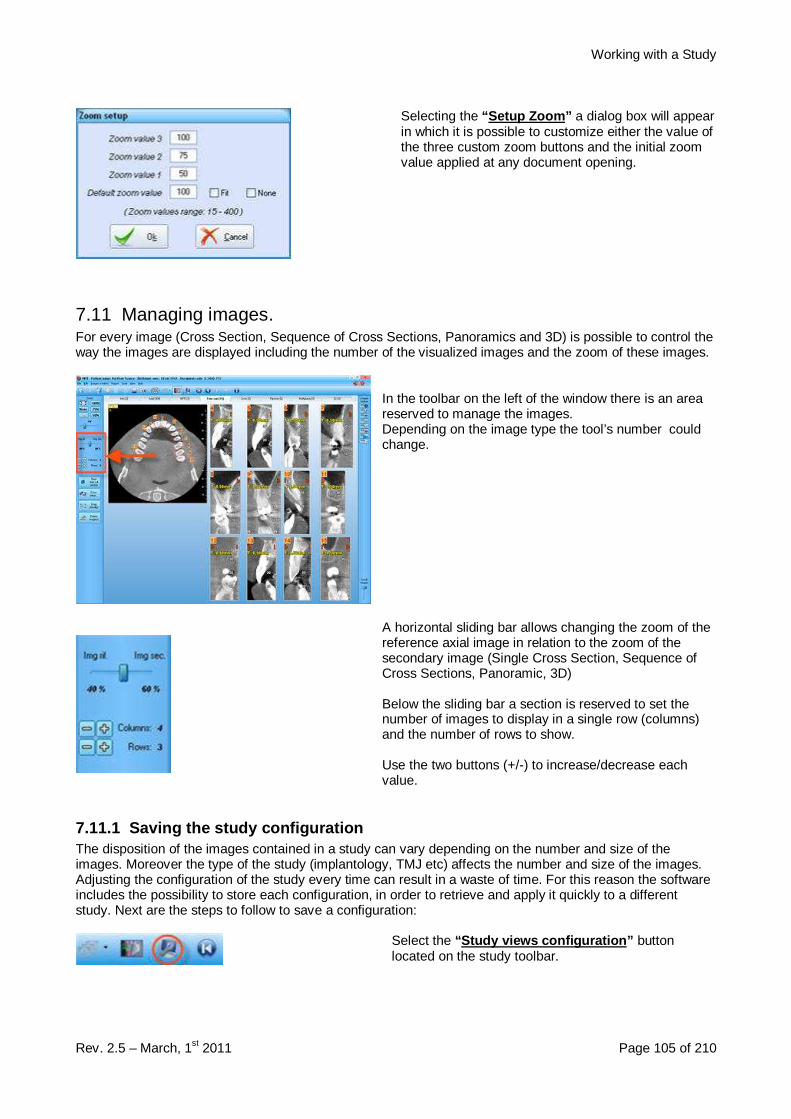
Working with a Study
Rev. 2.5 – March, 1st 2011 Page 105 of 210
Selecting the “Setup Zoom” a dialog box will appearin which it is possible to customize either the value ofthe three custom zoom buttons and the initial zoomvalue applied at any document opening.
7.11 Managing images.For every image (Cross Section, Sequence of Cross Sections, Panoramics and 3D) is possible to control theway the images are displayed including the number of the visualized images and the zoom of these images.
In the toolbar on the left of the window there is an areareserved to manage the images.Depending on the image type the tool’s number couldchange.
A horizontal sliding bar allows changing the zoom of thereference axial image in relation to the zoom of thesecondary image (Single Cross Section, Sequence ofCross Sections, Panoramic, 3D)
Below the sliding bar a section is reserved to set thenumber of images to display in a single row (columns)and the number of rows to show.
Use the two buttons (+/-) to increase/decrease eachvalue.
7.11.1 Saving the study configurationThe disposition of the images contained in a study can vary depending on the number and size of theimages. Moreover the type of the study (implantology, TMJ etc) affects the number and size of the images.Adjusting the configuration of the study every time can result in a waste of time. For this reason the softwareincludes the possibility to store each configuration, in order to retrieve and apply it quickly to a differentstudy. Next are the steps to follow to save a configuration:
Select the “ Study views configuration” buttonlocated on the study toolbar.
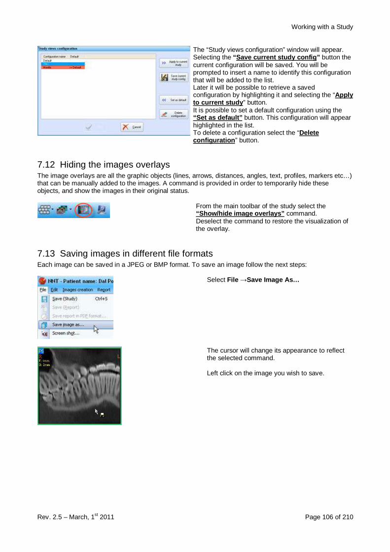
Working with a Study
Rev. 2.5 – March, 1st 2011 Page 106 of 210
The “Study views configuration” window will appear.Selecting the “Save current study config” button thecurrent configuration will be saved. You will beprompted to insert a name to identify this configurationthat will be added to the list.Later it will be possible to retrieve a savedconfiguration by highlighting it and selecting the “Applyto current study ” button.It is possible to set a default configuration using the“Set as default” button. This configuration will appearhighlighted in the list.To delete a configuration select the “Deleteconfiguration ” button.
7.12 Hiding the images overlaysThe image overlays are all the graphic objects (lines, arrows, distances, angles, text, profiles, markers etc…)that can be manually added to the images. A command is provided in order to temporarily hide theseobjects, and show the images in their original status.
From the main toolbar of the study select the“Show/hide image overlays” command.Deselect the command to restore the visualization ofthe overlay.
7.13 Saving images in different file formatsEach image can be saved in a JPEG or BMP format. To save an image follow the next steps:
Select File →Save Image As…
The cursor will change its appearance to reflectthe selected command.
Left click on the image you wish to save.
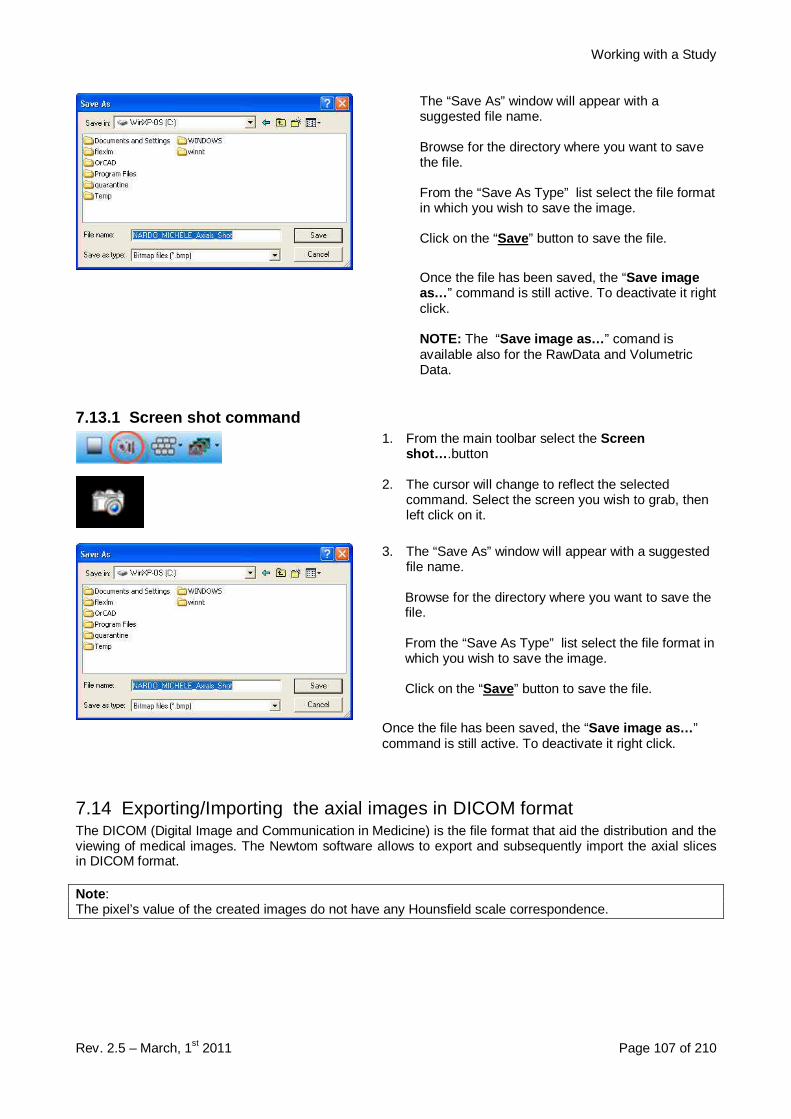
Working with a Study
Rev. 2.5 – March, 1st 2011 Page 107 of 210
The “Save As” window will appear with asuggested file name.
Browse for the directory where you want to savethe file.
From the “Save As Type” list select the file formatin which you wish to save the image.
Click on the “Save” button to save the file.
Once the file has been saved, the “Save imageas…” command is still active. To deactivate it rightclick.
NOTE: The “Save image as… ” comand isavailable also for the RawData and VolumetricData.
7.13.1 Screen shot command1. From the main toolbar select the Screen
shot… .button
2. The cursor will change to reflect the selectedcommand. Select the screen you wish to grab, thenleft click on it.
3. The “Save As” window will appear with a suggestedfile name.
Browse for the directory where you want to save thefile.
From the “Save As Type” list select the file format inwhich you wish to save the image.
Click on the “Save” button to save the file.
Once the file has been saved, the “Save image as… ”command is still active. To deactivate it right click.
7.14 Exporting/Importing the axial images in DICOM formatThe DICOM (Digital Image and Communication in Medicine) is the file format that aid the distribution and theviewing of medical images. The Newtom software allows to export and subsequently import the axial slicesin DICOM format.
Note :The pixel’s value of the created images do not have any Hounsfield scale correspondence.
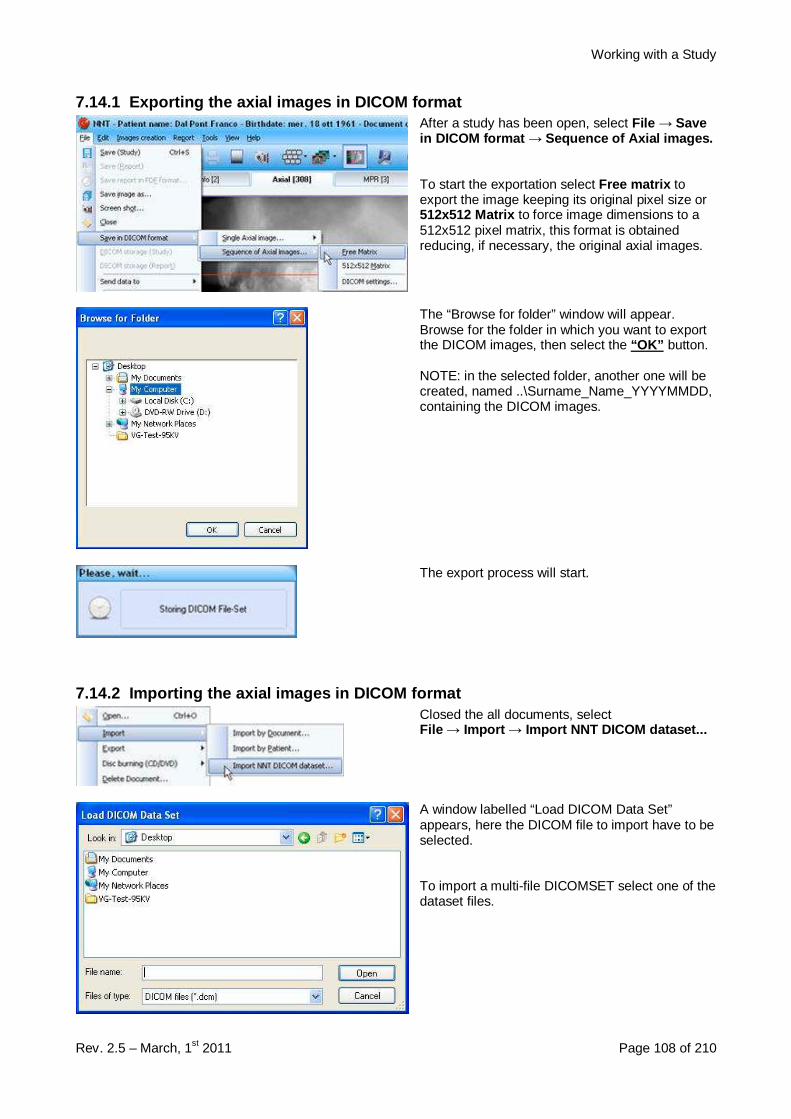
Working with a Study
Rev. 2.5 – March, 1st 2011 Page 108 of 210
7.14.1 Exporting the axial images in DICOM formatAfter a study has been open, select File → Savein DICOM format → Sequence of Axial images.
To start the exportation select Free matrix toexport the image keeping its original pixel size or512x512 Matrix to force image dimensions to a512x512 pixel matrix, this format is obtainedreducing, if necessary, the original axial images.
The “Browse for folder” window will appear.Browse for the folder in which you want to exportthe DICOM images, then select the “OK” button.
NOTE: in the selected folder, another one will becreated, named ..\Surname_Name_YYYYMMDD,containing the DICOM images.
The export process will start.
7.14.2 Importing the axial images in DICOM formatClosed the all documents, selectFile → Import → Import NNT DICOM dataset...
A window labelled “Load DICOM Data Set”appears, here the DICOM file to import have to beselected.
To import a multi-file DICOMSET select one of thedataset files.
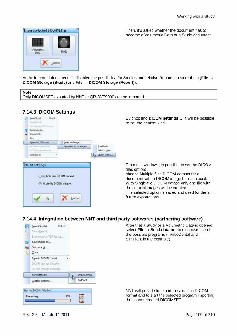
Working with a Study
Rev. 2.5 – March, 1st 2011 Page 109 of 210
Then, it’s asked whether the document has tobecome a Volumetric Data or a Study document.
At the imported documents is disabled the possibility, for Studies and relative Reports, to store them (File →DICOM Storage (Study) and File → DICOM Storage (Report) ).
Note :Only DICOMSET exported by NNT or QR-DVT9000 can be imported.
7.14.3 DICOM SettingsBy choosing DICOM settings… it will be possibleto set the dataset kind.
From this window it is possible to set the DICOMfiles option:choose Multiple files DICOM dataset for adocument with a DICOM image for each axial.With Single-file DICOM datase only one file withthe all axial images will be created.The selected option is saved and used for the allfuture exportations.
7.14.4 Integration between NNT and third party sof twares (partnering software)After that a Study or a Volumetric Data is openedselect File → Send data to , then choose one ofthe possible programs (InVivoDental andSimPlant in the example)
NNT will provide to export the axials in DICOMformat and to start the selected program importingthe sooner created DICOMSET.
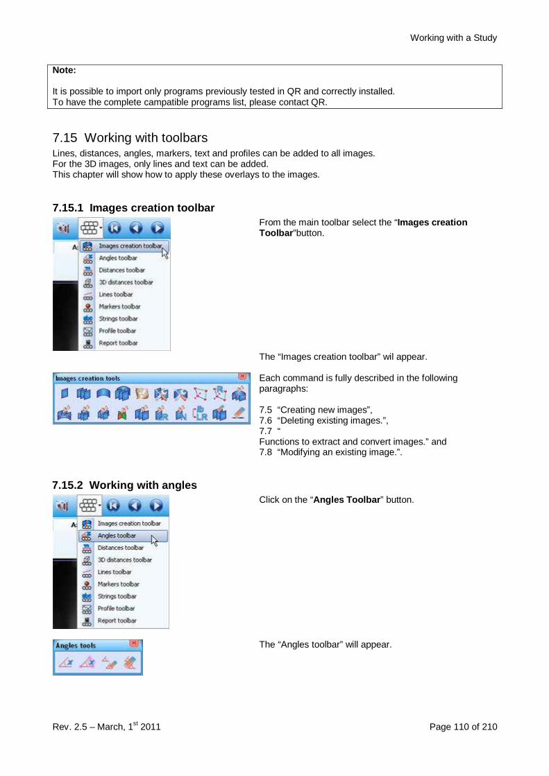
Working with a Study
Rev. 2.5 – March, 1st 2011 Page 110 of 210
Note:
It is possible to import only programs previously tested in QR and correctly installed.To have the complete campatible programs list, please contact QR.
7.15 Working with toolbarsLines, distances, angles, markers, text and profiles can be added to all images.For the 3D images, only lines and text can be added.This chapter will show how to apply these overlays to the images.
7.15.1 Images creation toolbarFrom the main toolbar select the “Images creationToolbar ”button.
The “Images creation toolbar” wil appear.
Each command is fully described in the followingparagraphs:
7.5 “Creating new images”,7.6 “Deleting existing images.”,7.7 “Functions to extract and convert images.” and7.8 “Modifying an existing image.”.
7.15.2 Working with anglesClick on the “Angles Toolbar ” button.
The “Angles toolbar” will appear.
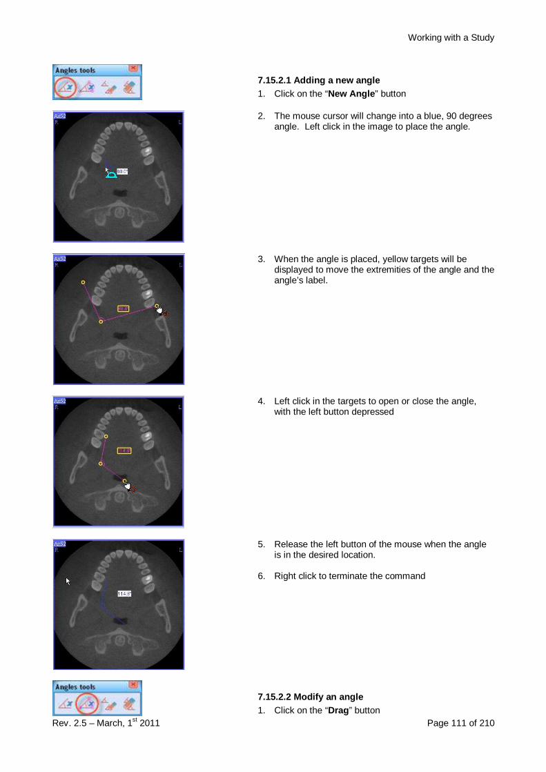
Working with a Study
Rev. 2.5 – March, 1st 2011 Page 111 of 210
7.15.2.1 Adding a new angle1. Click on the “New Angle ” button
2. The mouse cursor will change into a blue, 90 degreesangle. Left click in the image to place the angle.
3. When the angle is placed, yellow targets will bedisplayed to move the extremities of the angle and theangle’s label.
4. Left click in the targets to open or close the angle,with the left button depressed
5. Release the left button of the mouse when the angleis in the desired location.
6. Right click to terminate the command
7.15.2.2 Modify an angle1. Click on the “Drag ” button

Working with a Study
Rev. 2.5 – March, 1st 2011 Page 112 of 210
2. Yellow targets will be displayed to move theextremities of the angle and the angle’s label.
3. Left click in the targets to open or close the angle,keeping the left button of the mouse depressed.
4. Release the left button of the mouse when the targetsare in the desired location.
5. The label of the angle can be positioned by leftclicking in it and moving the mouse.
6. To terminate the command, right click
7.15.2.3 Delete an angle1. Click on the “Delete One Angle ” button
2. A yellow border will highlight the label of the angle.

Working with a Study
Rev. 2.5 – March, 1st 2011 Page 113 of 210
3. Left click inside the label to delete a specific angle.
4. Right click to finish.
7.15.2.4 Delete all angles1. Click on the “Delete All Angles ” button
2. Left click on the image where you want to remove allthe angles.
3. Right click to finish the command.
7.15.3 Working with lines and arrowsClick on the “Lines Toolbar” button.
The “Lines toolbar” will appear.
7.15.3.1 Trace a new line1. Click on the “New Line ” button.

Working with a Study
Rev. 2.5 – March, 1st 2011 Page 114 of 210
2. Left click in the image at the start point of thedistance.
3. Drag the line and left (or right) click at the end point ofthe distance.
4. To terminate the command, right click.
7.15.3.2 Trace a new line with text1. Click on the “New Line + Text ” button.
2. The “Text Editor” window will appear. Edit the text youwish to insert next to the line, then click on the “OK”button.
3. Left click in the image at the start point of thedistance.
4. Drag the line and left (or right) click at the end point ofthe distance.
5. Drag the text and left (or right) click in order to fix it.
6. To terminate the command, right click.

Working with a Study
Rev. 2.5 – March, 1st 2011 Page 115 of 210
7.15.3.3 Trace a new line with text from database1. Click on the “New Line + Text from DB ” button.
2. A window will appear showing the list of text in thedatabase.
3. Highlight a line of text then select one of the followingbuttons:
a) Apply as single line text : you will be ready to applythe text to the image as a single line.
b) Edit as single line text : the “Text editor” window willopen allowing you to modify the text before applying itas a single line to the image.
4. Left click in the image at the start point of thedistance.
5. Drag the line and left (or right) click at the end point ofthe distance.
6. Drag the text and left (or right) click in order to fix it.
7. To terminate the command, right click.
7.15.3.4 Trace a new arrow1. Click on the “New Arrow ” button.
2. Left click in the image where you want your arrow topoint.
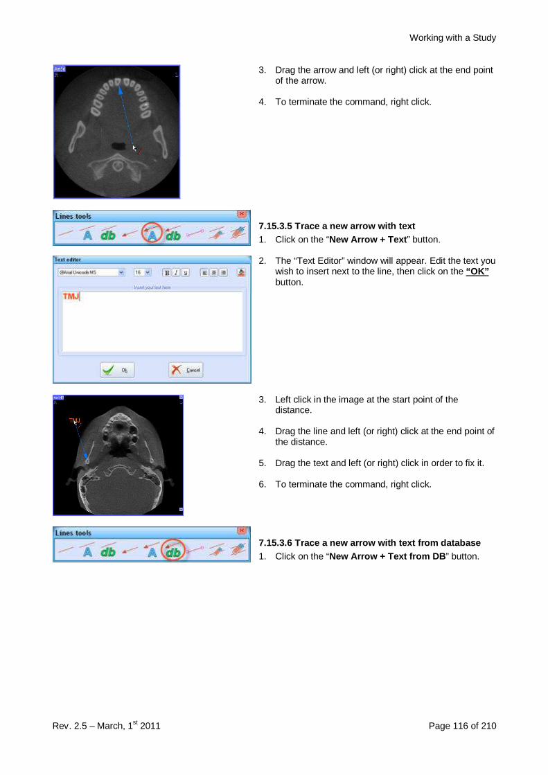
Working with a Study
Rev. 2.5 – March, 1st 2011 Page 116 of 210
3. Drag the arrow and left (or right) click at the end pointof the arrow.
4. To terminate the command, right click.
7.15.3.5 Trace a new arrow with text1. Click on the “New Arrow + Text ” button.
2. The “Text Editor” window will appear. Edit the text youwish to insert next to the line, then click on the “OK”button.
3. Left click in the image at the start point of thedistance.
4. Drag the line and left (or right) click at the end point ofthe distance.
5. Drag the text and left (or right) click in order to fix it.
6. To terminate the command, right click.
7.15.3.6 Trace a new arrow with text from database1. Click on the “New Arrow + Text from DB ” button.

Working with a Study
Rev. 2.5 – March, 1st 2011 Page 117 of 210
2. A window will appear showing the list of text in thedatabase.
3. Highlight a line of text then select one of the followingbuttons:
c) Apply as single line text : you will be ready to applythe text to the image as a single line.
d) Edit as single line text : the “Text editor” window willopen allowing you to modify the text before applying itas a single line to the image.
4. Left click in the image at the start point of thedistance.
5. Drag the line and left (or right) click at the end point ofthe distance.
6. Drag the text and left (or right) click in order to fix it.
7. To terminate the command, right click.
7.15.3.7 Modify a line or an arrow1. Click on the “Drag ” button.
2. Yellow target squares will be displayed to drag theline. Left click in the target and move the mouse withthe left mouse button depressed. The line color willbecome purple.

Working with a Study
Rev. 2.5 – March, 1st 2011 Page 118 of 210
3. Release the button when the line is at the desiredlocation.
4. To terminate the command, right click.
NOTE: In case a text has been inserted together with theline or arrow it will be possible to modify it by using thetext toolbar.
7.15.3.8 Deleting lines/arrows one at a time1. Click on the “Delete One Line ” button.
2. Yellow target squares will be displayed in order toselect the line to delete.
3. Left click in the target to delete the selected line.
4. To terminate the command, right click.
NOTE: In case a text has been inserted together with theline or arrow it will be possible to remove it by using thetext toolbar.
7.15.3.9 Deleting all lines and arrows1. Click on the “Delete all lines ” button.
2. Left click inside the image where you want to removeall the lines and/or arrows.
3. Right click to finish the command.
NOTE: In case a text has been inserted together with theline or arrow it will be possible to remove it by using thetext toolbar.

Working with a Study
Rev. 2.5 – March, 1st 2011 Page 119 of 210
7.15.4 Working with distancesClick on the “Distances Toolbar” button.
The “Distances toolbar” will appear.
7.15.4.1 Trace a new distance1. Click on the “New Distance ” button.
2. Left click in the image at the start point of thedistance.

Working with a Study
Rev. 2.5 – March, 1st 2011 Page 120 of 210
3. Drag the line and left (or right) click at the end point ofthe distance.
NOTE: In case the “Label auto positioning” flag (displayedin the “Graphic Options” window when the Distancesgroup is enabled) is unckeched, after the distance hasbeen traced you will be prompted to position the label bydragging it and left clicking with the mouse.
4. To terminate the command, right click.
7.15.4.2 Trace a new distance with arrow1. Click on the “New Distance (arrow) ” button.
2. Left click in the image at the start point of thedistance.
3. Drag the line and left (or right) click at the end point ofthe distance.
NOTE: In case the “Label auto positioning” flag (displayedin the “Graphic Options” window when the Distancesgroup is enabled) is unckeched, after the distance hasbeen traced you will be prompted to position the label bydragging it and left clicking with the mouse.
4. To terminate the command, right click.
7.15.4.3 Trace a new distance with hyphen1. Click on the “New Distance (hyphen) ” button.
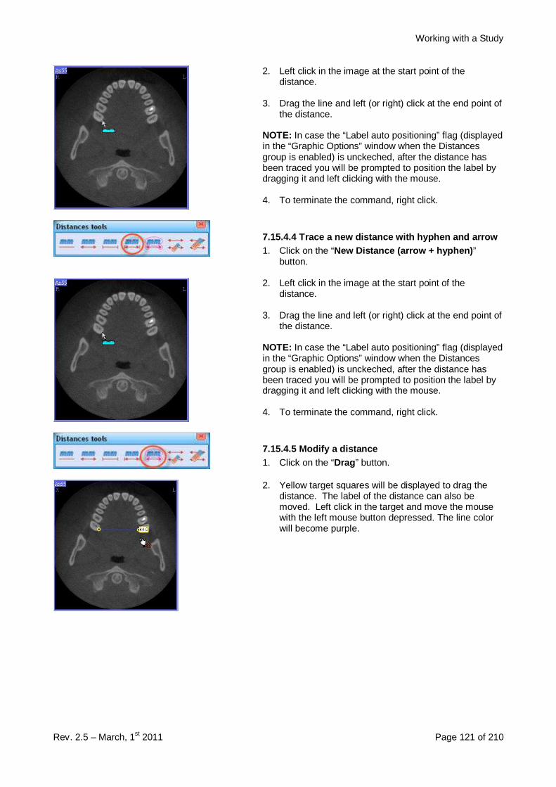
Working with a Study
Rev. 2.5 – March, 1st 2011 Page 121 of 210
2. Left click in the image at the start point of thedistance.
3. Drag the line and left (or right) click at the end point ofthe distance.
NOTE: In case the “Label auto positioning” flag (displayedin the “Graphic Options” window when the Distancesgroup is enabled) is unckeched, after the distance hasbeen traced you will be prompted to position the label bydragging it and left clicking with the mouse.
4. To terminate the command, right click.
7.15.4.4 Trace a new distance with hyphen and arrow1. Click on the “New Distance (arrow + hyphen) ”
button.
2. Left click in the image at the start point of thedistance.
3. Drag the line and left (or right) click at the end point ofthe distance.
NOTE: In case the “Label auto positioning” flag (displayedin the “Graphic Options” window when the Distancesgroup is enabled) is unckeched, after the distance hasbeen traced you will be prompted to position the label bydragging it and left clicking with the mouse.
4. To terminate the command, right click.
7.15.4.5 Modify a distance1. Click on the “Drag ” button.
2. Yellow target squares will be displayed to drag thedistance. The label of the distance can also bemoved. Left click in the target and move the mousewith the left mouse button depressed. The line colorwill become purple.
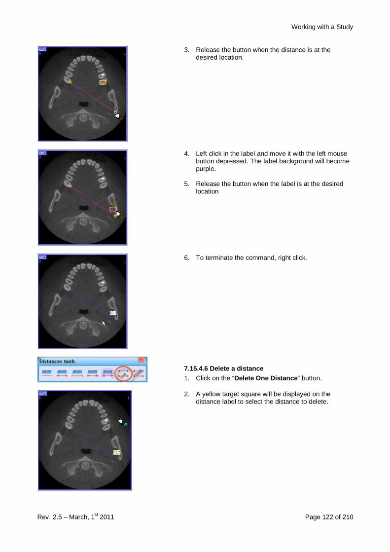
Working with a Study
Rev. 2.5 – March, 1st 2011 Page 122 of 210
3. Release the button when the distance is at thedesired location.
4. Left click in the label and move it with the left mousebutton depressed. The label background will becomepurple.
5. Release the button when the label is at the desiredlocation
6. To terminate the command, right click.
7.15.4.6 Delete a distance1. Click on the “Delete One Distance ” button.
2. A yellow target square will be displayed on thedistance label to select the distance to delete.

Working with a Study
Rev. 2.5 – March, 1st 2011 Page 123 of 210
3. Left click in the target to delete the selected distance.
4. To terminate the command, right click.
7.15.4.7 Delete all distances1. Click on the “Delete all distances ” button.
2. Left click inside the image where you want to removeall the distances.
3. Right click to finish the command.
7.15.5 Working with 3D distances
Click on the “3D Distances Toolbar” button.
The “3DDistance toolbar” will appear.
7.15.5.1 Trace a new 3D distance1. Click on the “New 3D Distance ” button.
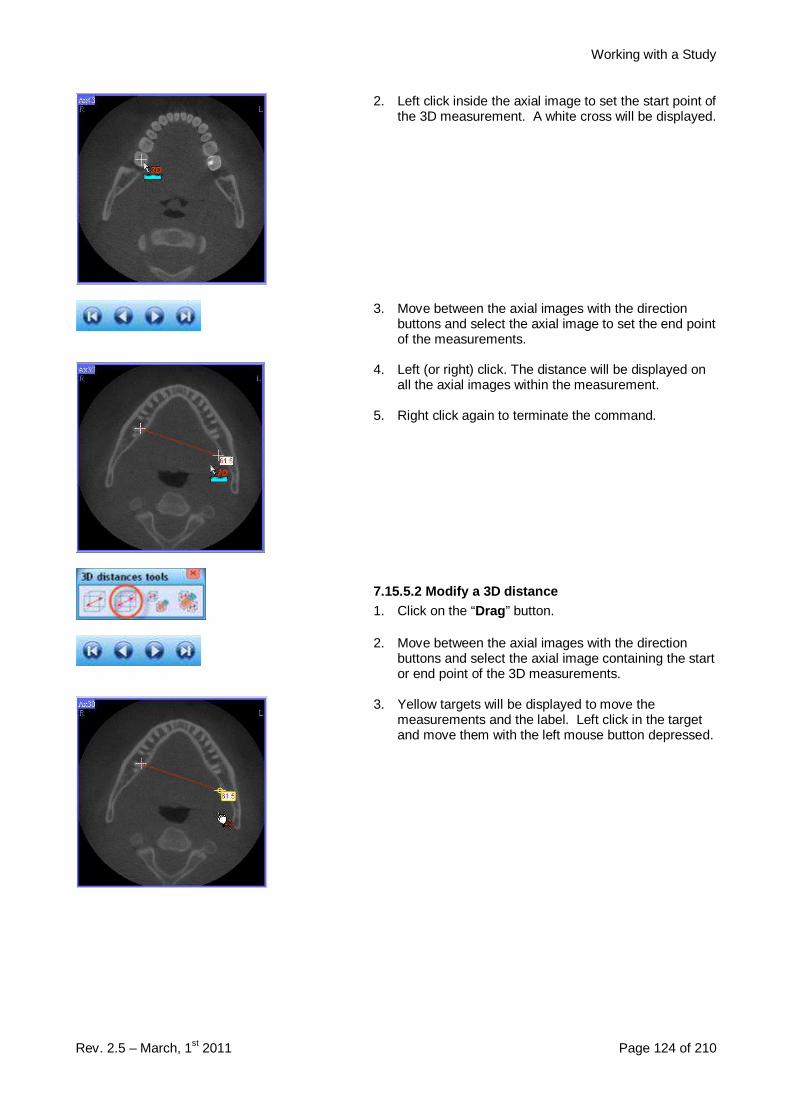
Working with a Study
Rev. 2.5 – March, 1st 2011 Page 124 of 210
2. Left click inside the axial image to set the start point ofthe 3D measurement. A white cross will be displayed.
3. Move between the axial images with the directionbuttons and select the axial image to set the end pointof the measurements.
4. Left (or right) click. The distance will be displayed onall the axial images within the measurement.
5. Right click again to terminate the command.
7.15.5.2 Modify a 3D distance1. Click on the “Drag ” button.
2. Move between the axial images with the directionbuttons and select the axial image containing the startor end point of the 3D measurements.
3. Yellow targets will be displayed to move themeasurements and the label. Left click in the targetand move them with the left mouse button depressed.
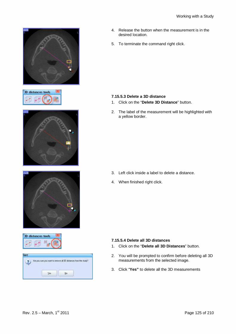
Working with a Study
Rev. 2.5 – March, 1st 2011 Page 125 of 210
4. Release the button when the measurement is in thedesired location.
5. To terminate the command right click.
7.15.5.3 Delete a 3D distance1. Click on the “Delete 3D Distance ” button.
2. The label of the measurement will be highlighted witha yellow border.
3. Left click inside a label to delete a distance.
4. When finished right click.
7.15.5.4 Delete all 3D distances1. Click on the “Delete all 3D Distances ” button.
2. You will be prompted to confirm before deleting all 3Dmeasurements from the selected image.
3. Click “Yes” to delete all the 3D measurements

Working with a Study
Rev. 2.5 – March, 1st 2011 Page 126 of 210
7.15.6 Working with markersThe marker is a graphic object that can be traced on axial, cross section and panoramic images (having athickness lower than 1 mm). Once the marker has been traced it will be reported on all the images that crossits path (with the exception of 3D images).
The typical usage of the marker is highlighting the path of the mandibular canal in the panoramic image, andrecognize its position in the cross sections.
Click on the “Markers Toolbar” button.
The “Markers toolbar” will appear.
7.15.6.1 Trace a small marker1. Click on the “New Small Marker ” button.
2. Trace the path of the marker left clicking while movingthe mouse.
3. To terminate the command right click.
7.15.6.2 Trace a medium marker1. Click on the “New Medium Marker ” button
2. Trace the path of the marker left clicking while movingthe mouse.
3. To terminate the command right click.
7.15.6.3 Trace a large marker1. Click on the “New Large Marker ” button.

Working with a Study
Rev. 2.5 – March, 1st 2011 Page 127 of 210
2. Trace the path of the marker left clicking while movingthe mouse.
3. To terminate the command right click.
7.15.6.4 Change the marker color1. Click on the “Change Default Marker color ”button.
2. The “Color” window will open. Select the desired colorfor the marker and click on the “OK” button.
7.15.6.5 Hide all the markers in the study1. Click on the “Hide All Markers ” button.
2. All the markers in the study will be hidden (to restorethe markers after they have been hidden, click againon the “Hide All Markers” button).
7.15.6.6 Delete a marker1. Click on the “Delete Marker ” button.
2. Select the marker to be deleted.
7.15.6.7 Delete all the markers from the study1. Click on the “Delete All Markers ” button.
2. You will be prompted to confirm before deleting all themarkers from the study. Select the “Yes” button.
3. All the markers will be removed from the study (Usethis command with caution! ).
7.15.7 Working with profilesA profile reports the value of each data point of an image on a scale from 0-65535.
Click on the “Profile Toolbar” button.
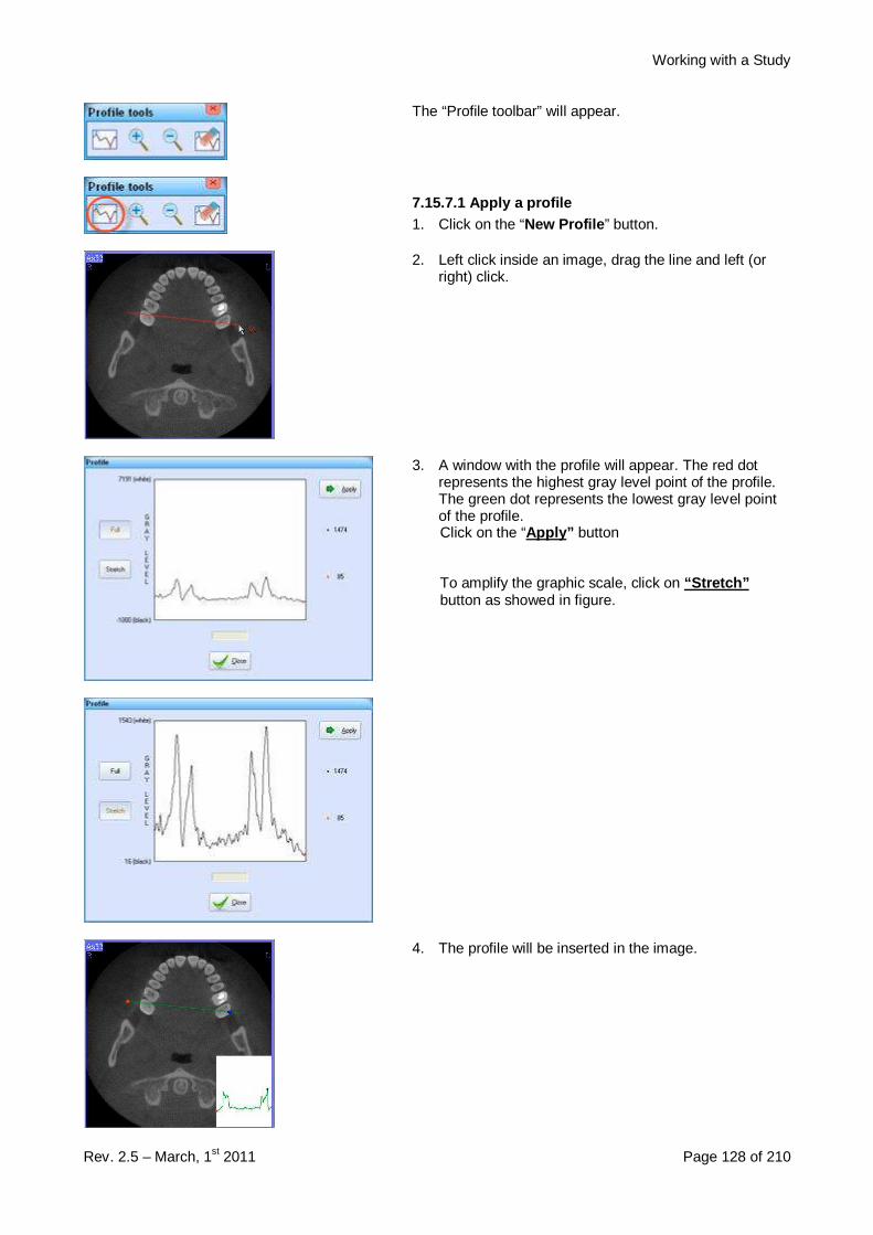
Working with a Study
Rev. 2.5 – March, 1st 2011 Page 128 of 210
The “Profile toolbar” will appear.
7.15.7.1 Apply a profile1. Click on the “New Profile ” button.
2. Left click inside an image, drag the line and left (orright) click.
3. A window with the profile will appear. The red dotrepresents the highest gray level point of the profile.The green dot represents the lowest gray level pointof the profile.Click on the “Apply” button
To amplify the graphic scale, click on “Stretch”button as showed in figure.
4. The profile will be inserted in the image.

Working with a Study
Rev. 2.5 – March, 1st 2011 Page 129 of 210
7.15.7.2 Increase the zoom of a profile1. Click on the “Zoom+ ” button.
2. Left click inside the image where you have applied theprofile.The graph of the profile will increase its size.
3. Right click to terminate the command.
7.15.7.3 Decrease the zoom of a profile1. Click on the “Zoom- ” button.
2. Left click inside the image where you have applied theprofile.The graph of the profile will decrease its size.
3. Right click to terminate the command.
7.15.7.4 Delete a profile1. Click on the “Delete Profile ” button.
2. Left click inside the image where you want to deletethe profile.
3. The profile will be removed from the image.
7.15.8 Working with textText can be apply to all the images in different ways
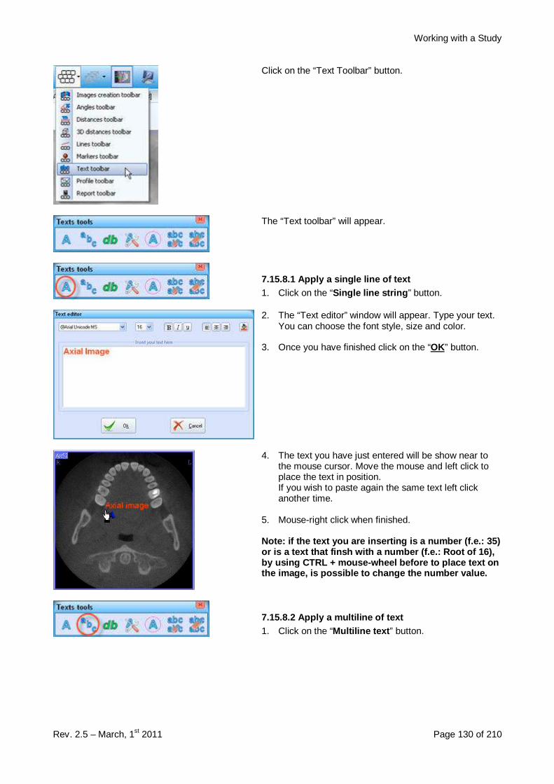
Working with a Study
Rev. 2.5 – March, 1st 2011 Page 130 of 210
Click on the “Text Toolbar” button.
The “Text toolbar” will appear.
7.15.8.1 Apply a single line of text1. Click on the “Single line string ” button.
2. The “Text editor” window will appear. Type your text.You can choose the font style, size and color.
3. Once you have finished click on the “OK” button.
4. The text you have just entered will be show near tothe mouse cursor. Move the mouse and left click toplace the text in position.If you wish to paste again the same text left clickanother time.
5. Mouse-right click when finished.
Note: if the text you are inserting is a number (f. e.: 35)or is a text that finsh with a number (f.e.: Root of 16 ),by using CTRL + mouse-wheel before to place text onthe image, is possible to change the number value.
7.15.8.2 Apply a multiline of text1. Click on the “Multiline text ” button.
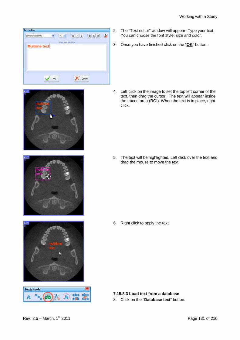
Working with a Study
Rev. 2.5 – March, 1st 2011 Page 131 of 210
2. The “Text editor” window will appear. Type your text.You can choose the font style, size and color.
3. Once you have finished click on the “OK” button.
4. Left click on the image to set the top left corner of thetext, then drag the cursor. The text will appear insidethe traced area (ROI). When the text is in place, rightclick.
5. The text will be highlighted. Left click over the text anddrag the mouse to move the text.
6. Right click to apply the text.
7.15.8.3 Load text from a database8. Click on the “Database text ” button.
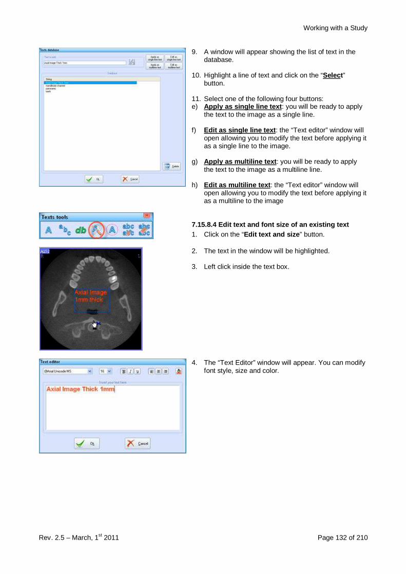
Working with a Study
Rev. 2.5 – March, 1st 2011 Page 132 of 210
9. A window will appear showing the list of text in thedatabase.
10. Highlight a line of text and click on the “Select ”button.
11. Select one of the following four buttons:e) Apply as single line text : you will be ready to apply
the text to the image as a single line.
f) Edit as single line text : the “Text editor” window willopen allowing you to modify the text before applying itas a single line to the image.
g) Apply as multiline text : you will be ready to applythe text to the image as a multiline line.
h) Edit as multiline text : the “Text editor” window willopen allowing you to modify the text before applying itas a multiline to the image
7.15.8.4 Edit text and font size of an existing tex t1. Click on the “Edit text and size ” button.
2. The text in the window will be highlighted.
3. Left click inside the text box.
4. The “Text Editor” window will appear. You can modifyfont style, size and color.

Working with a Study
Rev. 2.5 – March, 1st 2011 Page 133 of 210
5. Once you have completed your changes, click on the“OK” button.
6. The modified text will appear highlighted. Use themouse to change the size and the position of the boxthat contains the text.
7. Right click to apply the changes.
7.15.8.5 Moving text1. Click on the “Drag text ” button.
2. The text will appear highlighted. Use the mouse tochange the size and the position of the box thatcontains the text.

Working with a Study
Rev. 2.5 – March, 1st 2011 Page 134 of 210
3. Once you have moved the text right click to close thecommand.
7.15.8.6 Delete a line of text1. Click on the “Delete one text ” button.
2. A blue box will appear around each text.
3. Move the cursor over the text to highlight it and thenleft click to delete it.
7.15.8.7 Delete all the text from an image1. Click on the “Delete all texts ” button.
2. Left click over the image from which you want todelete all the text.
3. Right click to deselect the command.
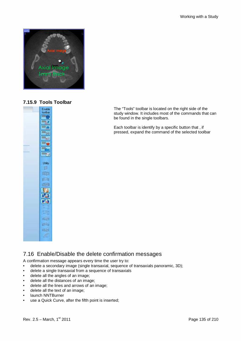
Working with a Study
Rev. 2.5 – March, 1st 2011 Page 135 of 210
7.15.9 Tools ToolbarThe “Tools” toolbar is located on the right side of thestudy window. It includes most of the commands that canbe found in the single toolbars.
Each toolbar is identify by a specific button that , ifpressed, expand the command of the selected toolbar
7.16 Enable/Disable the delete confirmation messagesA confirmation message appears every time the user try to:• delete a secondary image (single transaxial, sequence of transaxials panoramic, 3D);• delete a single transaxial from a sequence of transaxials• delete all the angles of an image;• delete all the distances of an image;• delete all the lines and arrows of an image;• delete all the text of an image;• launch NNTBurner• use a Quick Curve, after the fifth point is inserted;
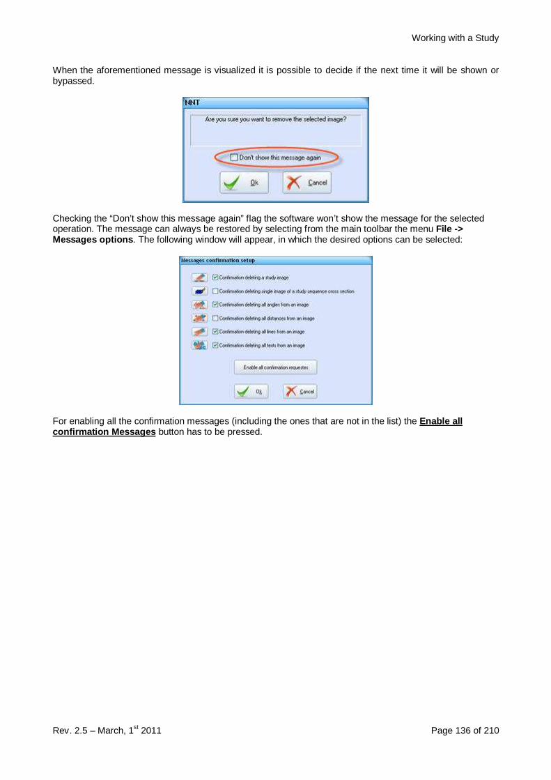
Working with a Study
Rev. 2.5 – March, 1st 2011 Page 136 of 210
When the aforementioned message is visualized it is possible to decide if the next time it will be shown orbypassed.
Checking the “Don’t show this message again” flag the software won’t show the message for the selectedoperation. The message can always be restored by selecting from the main toolbar the menu File ->Messages options . The following window will appear, in which the desired options can be selected:
For enabling all the confirmation messages (including the ones that are not in the list) the Enable allconfirmation Messages button has to be pressed.
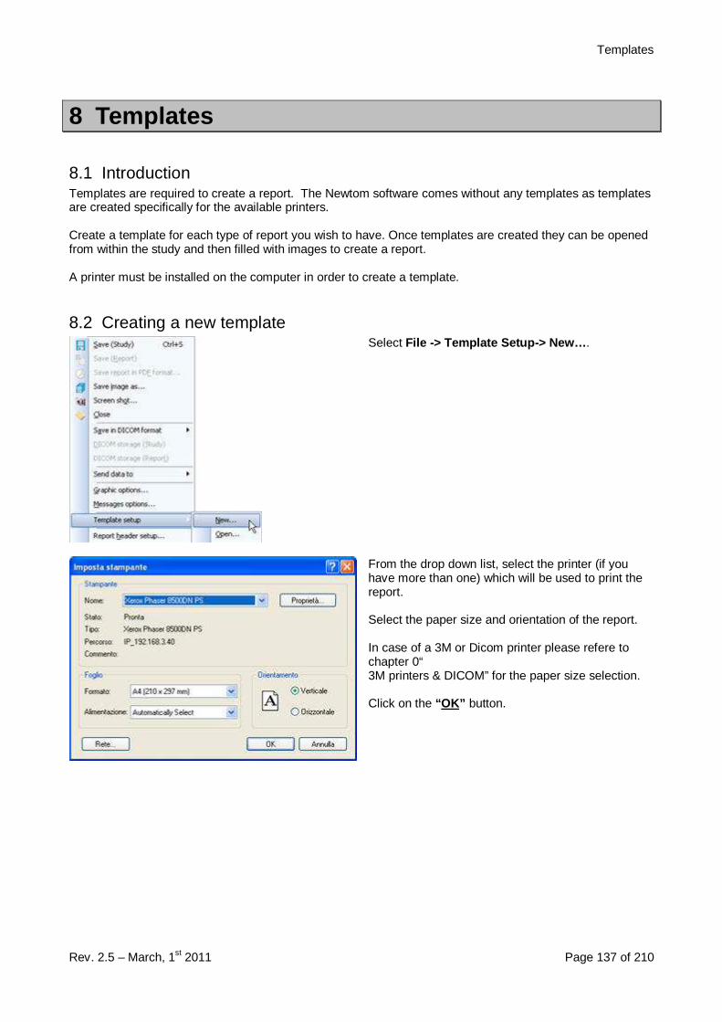
Templates
Rev. 2.5 – March, 1st 2011 Page 137 of 210
8 Templates
8.1 IntroductionTemplates are required to create a report. The Newtom software comes without any templates as templatesare created specifically for the available printers.
Create a template for each type of report you wish to have. Once templates are created they can be openedfrom within the study and then filled with images to create a report.
A printer must be installed on the computer in order to create a template.
8.2 Creating a new templateSelect File -> Template Setup-> New… .
From the drop down list, select the printer (if youhave more than one) which will be used to print thereport.
Select the paper size and orientation of the report.
In case of a 3M or Dicom printer please refere tochapter 0“3M printers & DICOM” for the paper size selection.
Click on the “ OK” button.
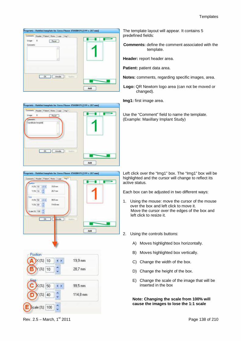
Templates
Rev. 2.5 – March, 1st 2011 Page 138 of 210
The template layout will appear. It contains 5predefined fields:
Comments: define the comment associated with thetemplate.
Header : report header area.
Patient : patient data area.
Notes : comments, regarding specific images, area.
Logo : QR Newtom logo area (can not be moved orchanged).
Img1 : first image area.
Use the “Comment” field to name the template.(Example: Maxillary Implant Study)
Left click over the “Img1” box. The “Img1” box will behighlighted and the cursor will change to reflect itsactive status.
Each box can be adjusted in two different ways:
1. Using the mouse: move the cursor of the mouseover the box and left click to move it.Move the cursor over the edges of the box andleft click to resize it.
2. Using the controls buttons:
A) Moves highlighted box horizontally.
B) Moves highlighted box vertically.
C) Change the width of the box.
D) Change the height of the box.
E) Change the scale of the image that will beinserted in the box
Note: Changing the scale from 100% willcause the images to lose the 1:1 scale

Templates
Rev. 2.5 – March, 1st 2011 Page 139 of 210
Position and resize the box as you wish.
Click on the “ Add ” button to add a new image box.
Adjust the new image box’s size and position.
Continue adding new image fields until finished withthe template.
Click on the “Remov e” button to delete thehighlighted box.
Click on the “ OK” button.
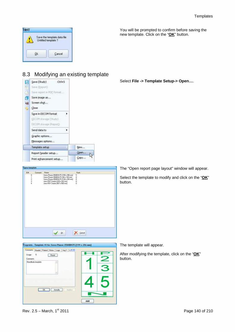
Templates
Rev. 2.5 – March, 1st 2011 Page 140 of 210
You will be prompted to confirm before saving thenew template. Click on the “OK” button.
8.3 Modifying an existing templateSelect File -> Template Setup-> Open… .
The “Open report page layout” window will appear.
Select the template to modify and click on the “OK”button.
The template will appear.
After modifying the template, click on the “OK”button.

Templates
Rev. 2.5 – March, 1st 2011 Page 141 of 210
You will be prompted to confirm before saving thechanges to the template.
Click on the “OK” button.
8.4 Deleting templatesSelect File -> Template Setup-> Delete… .
The “Delete report page layout” window will appear.
Select the template to delete and click on the “OK”button.
You will be prompted to confirm before deleting thetemplate.
Click on the “Yes” button to delete the template.
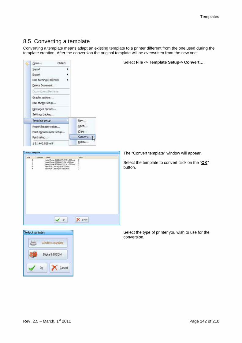
Templates
Rev. 2.5 – March, 1st 2011 Page 142 of 210
8.5 Converting a templateConverting a template means adapt an existing template to a printer different from the one used during thetemplate creation. After the conversion the original template will be overwritten from the new one.
Select File -> Template Setup-> Convert… .
The “Convert template” window will appear.
Select the template to convert click on the “OK”button.
Select the type of printer you wish to use for theconversion.
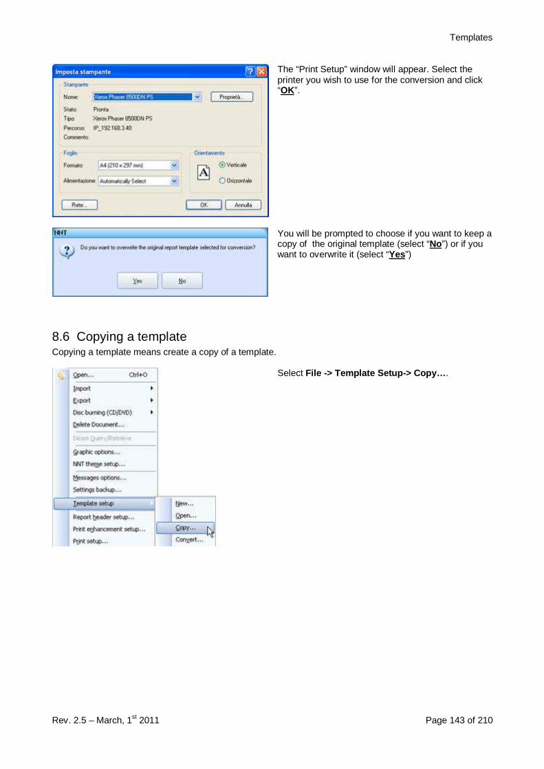
Templates
Rev. 2.5 – March, 1st 2011 Page 143 of 210
The “Print Setup” window will appear. Select theprinter you wish to use for the conversion and click“OK”.
You will be prompted to choose if you want to keep acopy of the original template (select “No”) or if youwant to overwrite it (select “Yes”)
8.6 Copying a templateCopying a template means create a copy of a template.
Select File -> Template Setup-> Copy… .
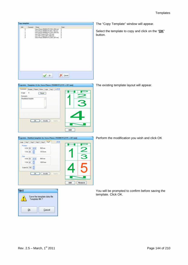
Templates
Rev. 2.5 – March, 1st 2011 Page 144 of 210
The “Copy Template” window will appear.
Select the template to copy and click on the “OK”button.
The existing template layout will appear.
Perform the modification you wish and click OK
You will be prompted to confirm before saving thetemplate. Click OK.
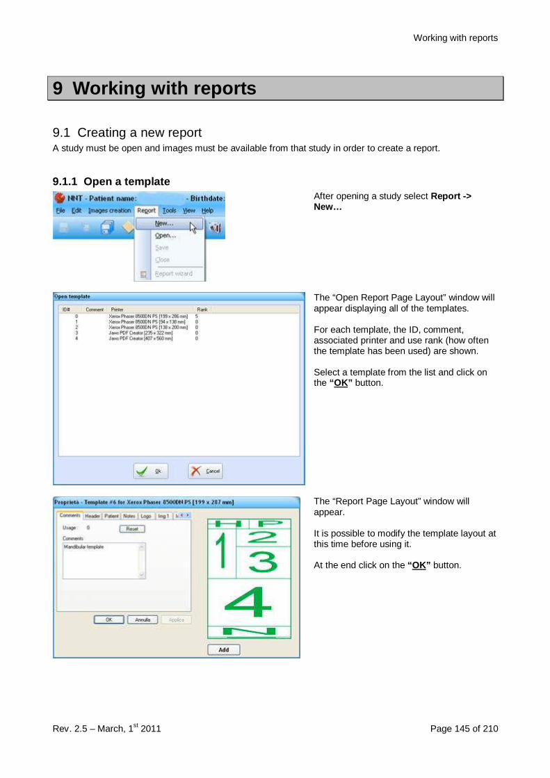
Working with reports
Rev. 2.5 – March, 1st 2011 Page 145 of 210
9 Working with reports
9.1 Creating a new reportA study must be open and images must be available from that study in order to create a report.
9.1.1 Open a templateAfter opening a study select Report ->New…
The “Open Report Page Layout” window willappear displaying all of the templates.
For each template, the ID, comment,associated printer and use rank (how oftenthe template has been used) are shown.
Select a template from the list and click onthe “ OK” button.
The “Report Page Layout” window willappear.
It is possible to modify the template layout atthis time before using it.
At the end click on the “ OK” button.
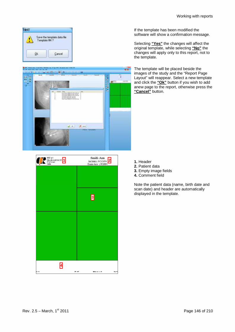
Working with reports
Rev. 2.5 – March, 1st 2011 Page 146 of 210
If the template has been modified thesoftware will show a confirmation message.
Selecting “Yes” the changes will affect theoriginal template, while selecting “No” thechanges will apply only to this report, not tothe template.
The template will be placed beside theimages of the study and the “Report PageLayout” will reappear. Select a new templateand click the “Ok” button if you wish to addanew page to the report, otherwise press the“Cancel” button.
1 2
3
4
1. Header2. Patient data3. Empty image fields4. Comment field
Note the patient data (name, birth date andscan date) and header are automaticallydisplayed in the template.
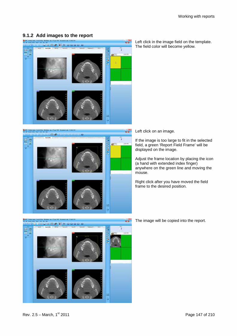
Working with reports
Rev. 2.5 – March, 1st 2011 Page 147 of 210
9.1.2 Add images to the reportLeft click in the image field on the template.The field color will become yellow.
Left click on an image.
If the image is too large to fit in the selectedfield, a green ‘Report Field Frame’ will bedisplayed on the image.
Adjust the frame location by placing the icon(a hand with extended index finger)anywhere on the green line and moving themouse.
Right click after you have moved the fieldframe to the desired position.
The image will be copied into the report.
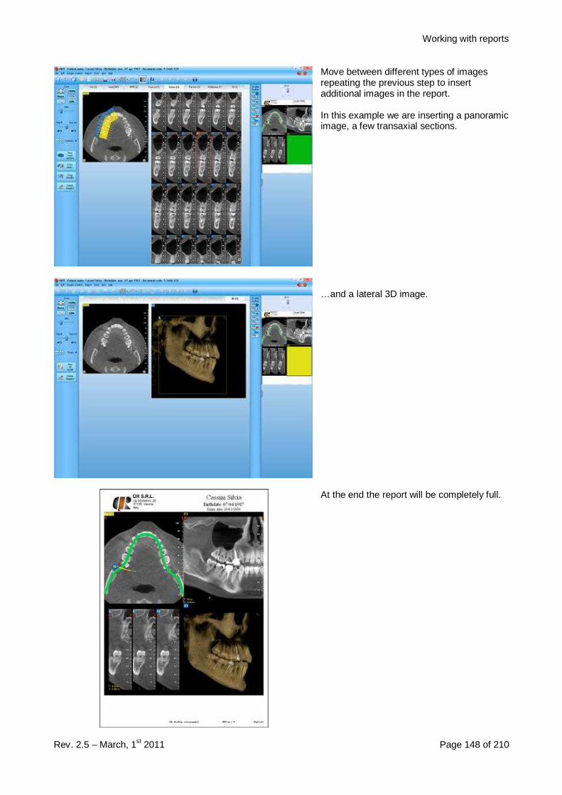
Working with reports
Rev. 2.5 – March, 1st 2011 Page 148 of 210
Move between different types of imagesrepeating the previous step to insertadditional images in the report.
In this example we are inserting a panoramicimage, a few transaxial sections.
…and a lateral 3D image.
At the end the report will be completely full.
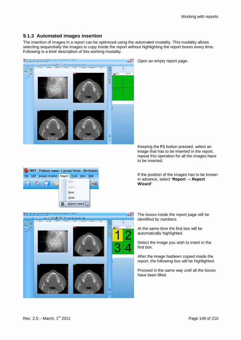
Working with reports
Rev. 2.5 – March, 1st 2011 Page 149 of 210
9.1.3 Automated images insertionThe insertion of images in a report can be optimized using the automated modality. This modality allowsselecting sequentially the images to copy inside the report without highlighting the report boxes every time.Following is a brief description of this working modality.
Open an empty report page.
Keeping the F1 button pressed, select animage that has to be inserted in the report,repeat this operation for all the images haveto be inserted.
If the position of the images has to be knownin advance, select “Report → ReportWizard ”
The boxes inside the report page will beidentified by numbers.
At the same time the first box will beautomatically highlighted.
Select the image you wish to insert in thefirst box.
After the image hasbeen copied inside thereport, the following box will be highlighted.
Proceed in the same way until all the boxeshave been filled.

Working with reports
Rev. 2.5 – March, 1st 2011 Page 150 of 210
9.1.4 Delete images from a reportTo delete an image from the report, rightclick on the image in the report.
A pop-up menu will appear.
Click on the “Remove ” menu item.
A red cross will be drawn on the selectedimage.
You will be prompted to confirm beforedeleting the image.
Click on Yes to delete the image.
9.1.5 Insert notes in the reportBe sure a note field has been designatedwithin the report.
Left click on the report to enable it.
Select Edit -> Report Page Notes…
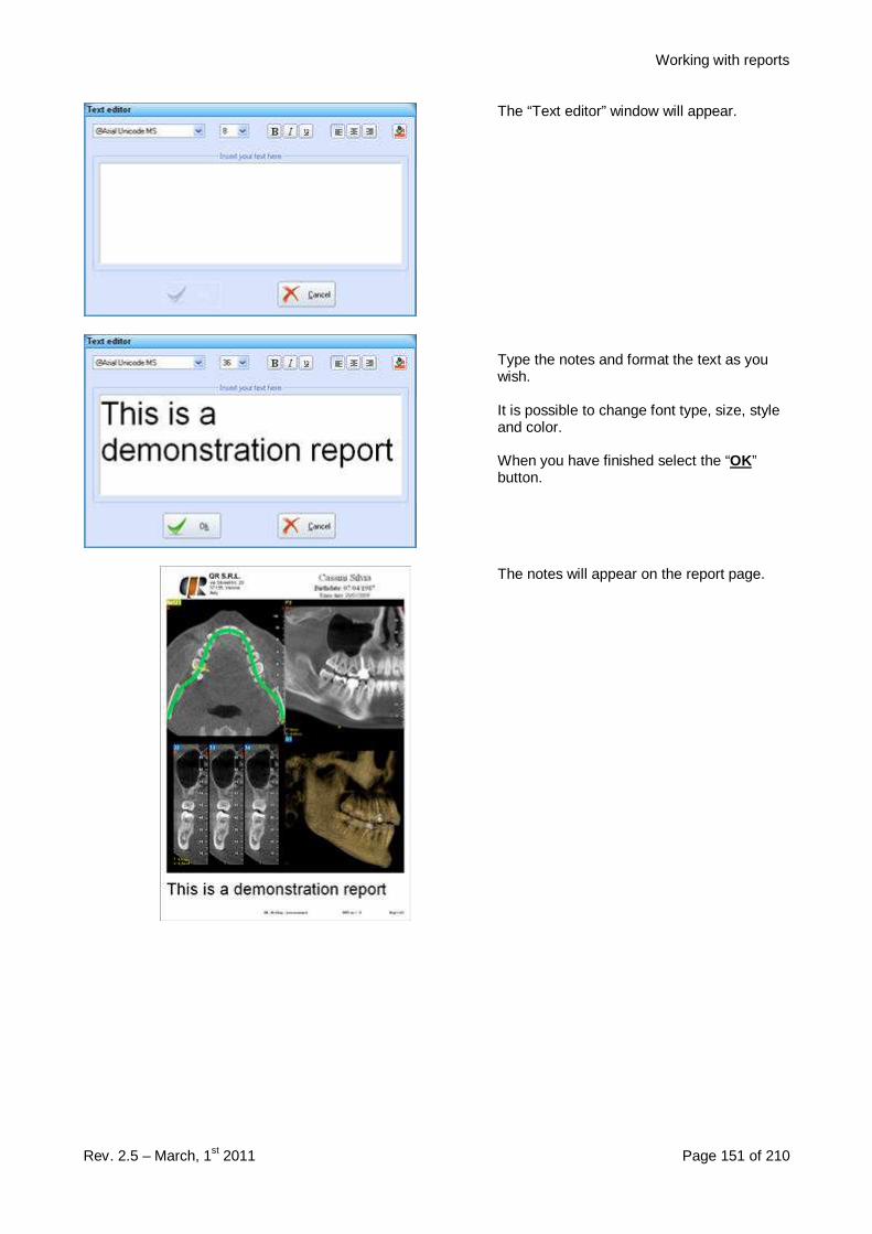
Working with reports
Rev. 2.5 – March, 1st 2011 Page 151 of 210
The “Text editor” window will appear.
Type the notes and format the text as youwish.
It is possible to change font type, size, styleand color.
When you have finished select the “OK”button.
The notes will appear on the report page.
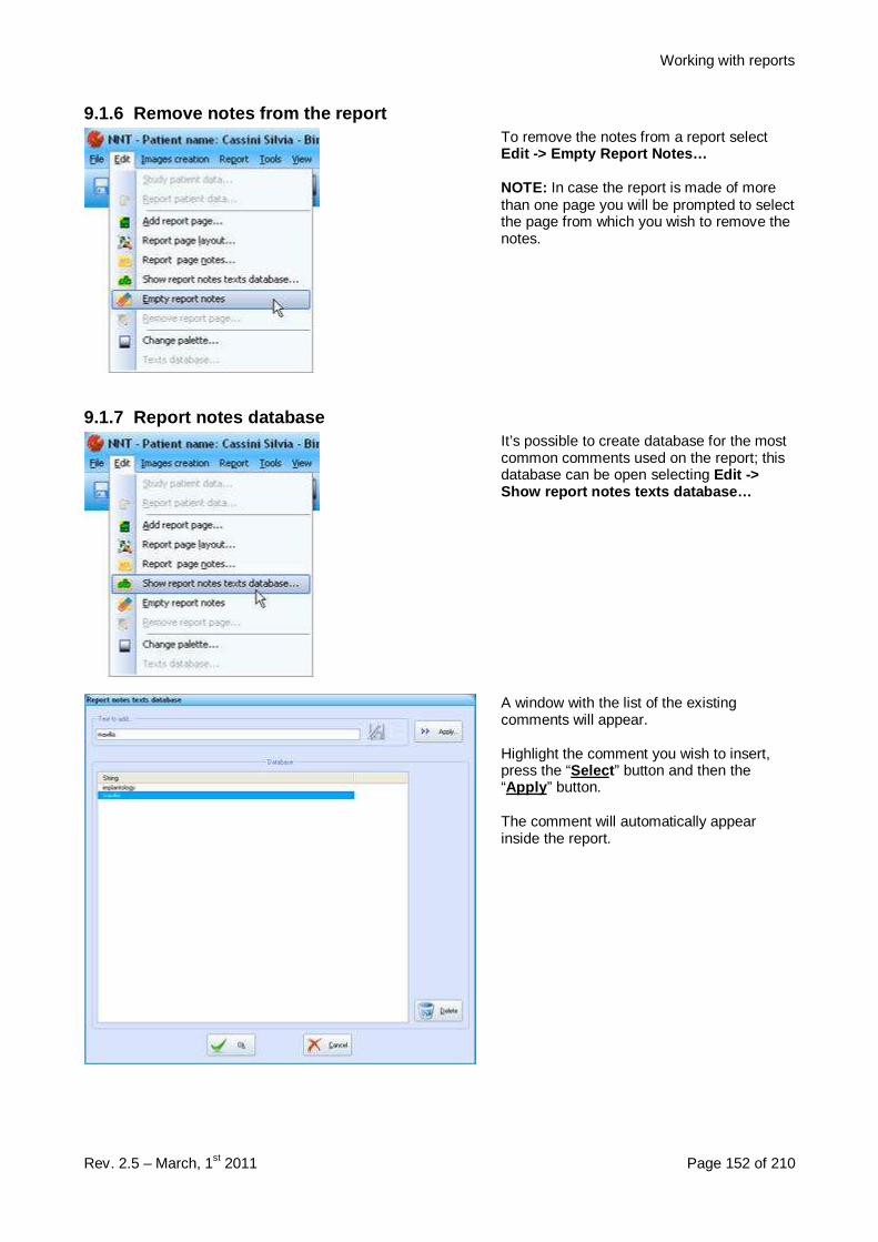
Working with reports
Rev. 2.5 – March, 1st 2011 Page 152 of 210
9.1.6 Remove notes from the reportTo remove the notes from a report selectEdit -> Empty Report Notes…
NOTE: In case the report is made of morethan one page you will be prompted to selectthe page from which you wish to remove thenotes.
9.1.7 Report notes databaseIt’s possible to create database for the mostcommon comments used on the report; thisdatabase can be open selecting Edit ->Show report notes texts database…
A window with the list of the existingcomments will appear.
Highlight the comment you wish to insert,press the “Select ” button and then the“Apply ” button.
The comment will automatically appearinside the report.
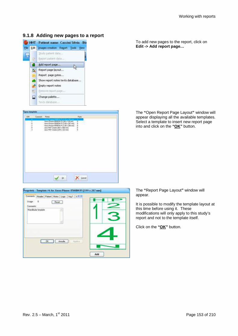
Working with reports
Rev. 2.5 – March, 1st 2011 Page 153 of 210
9.1.8 Adding new pages to a reportTo add new pages to the report, click onEdit -> Add report page…
The “ Open Report Page Layout” window willappear displaying all the available templates.Select a template to insert new report pageinto and click on the “ OK” button.
The “ Report Page Layout” window willappear.
It is possible to modify the template layout atthis time before using it. Thesemodifications will only apply to this study’sreport and not to the template itself.
Click on the “ OK” button.
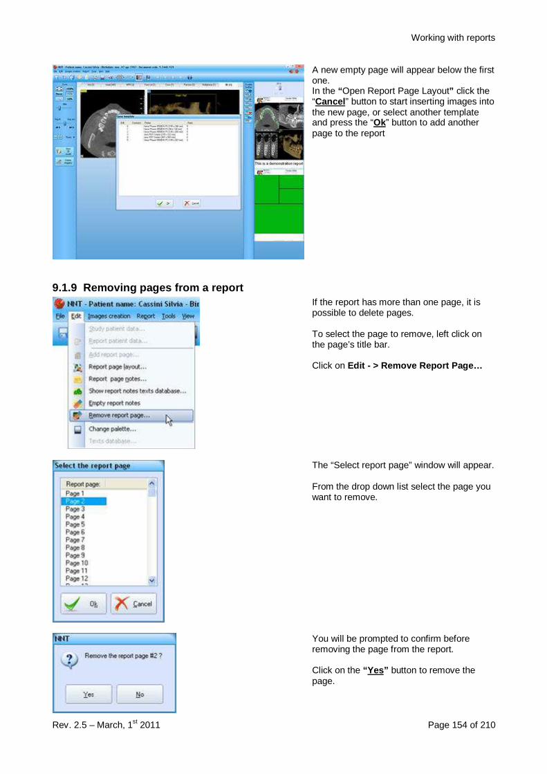
Working with reports
Rev. 2.5 – March, 1st 2011 Page 154 of 210
A new empty page will appear below the firstone.In the “ Open Report Page Layout” click the“Cancel ” button to start inserting images intothe new page, or select another templateand press the “Ok” button to add anotherpage to the report
9.1.9 Removing pages from a reportIf the report has more than one page, it ispossible to delete pages.
To select the page to remove, left click onthe page’s title bar.
Click on Edit - > Remove Report Page…
The “Select report page” window will appear.
From the drop down list select the page youwant to remove.
You will be prompted to confirm beforeremoving the page from the report.
Click on the “ Yes” button to remove thepage.
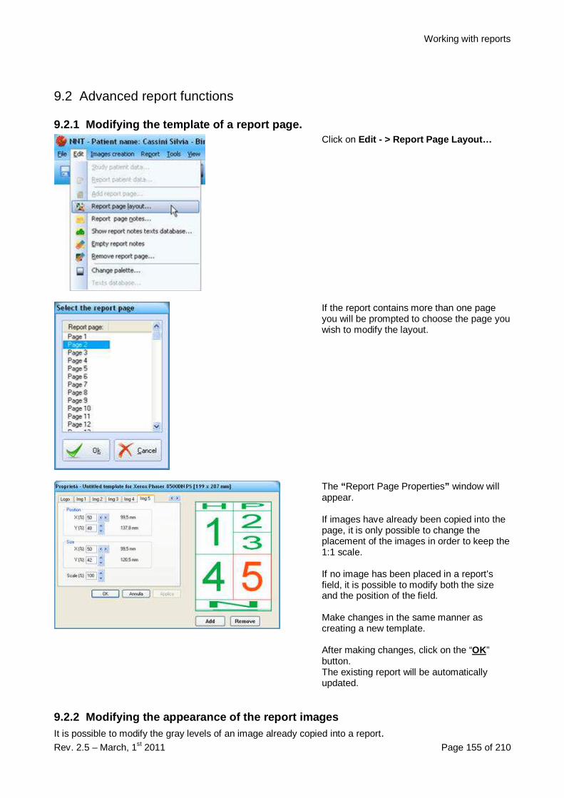
Working with reports
Rev. 2.5 – March, 1st 2011 Page 155 of 210
9.2 Advanced report functions
9.2.1 Modifying the template of a report page.Click on Edit - > Report Page Layout…
If the report contains more than one pageyou will be prompted to choose the page youwish to modify the layout.
The “ Report Page Properties” window willappear.
If images have already been copied into thepage, it is only possible to change theplacement of the images in order to keep the1:1 scale.
If no image has been placed in a report’sfield, it is possible to modify both the sizeand the position of the field.
Make changes in the same manner ascreating a new template.
After making changes, click on the “OK”button.The existing report will be automaticallyupdated.
9.2.2 Modifying the appearance of the report image sIt is possible to modify the gray levels of an image already copied into a report.
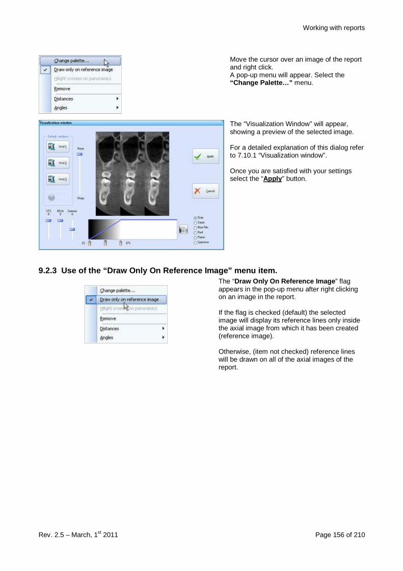
Working with reports
Rev. 2.5 – March, 1st 2011 Page 156 of 210
Move the cursor over an image of the reportand right click.A pop-up menu will appear. Select the“ Change Palette… ” menu.
The “Visualization Window” will appear,showing a preview of the selected image.
For a detailed explanation of this dialog referto 7.10.1 “Visualization window”.
Once you are satisfied with your settingsselect the “Apply ” button.
9.2.3 Use of the “Draw Only On Reference Image” me nu item.The “Draw Only On Reference Image ” flagappears in the pop-up menu after right clickingon an image in the report.
If the flag is checked (default) the selectedimage will display its reference lines only insidethe axial image from which it has been created(reference image).
Otherwise, (item not checked) reference lineswill be drawn on all of the axial images of thereport.

Working with reports
Rev. 2.5 – March, 1st 2011 Page 157 of 210
Axial image without reference lines
Axial image with reference lines
9.2.4 Use of the “Highlight crosses on panoramics” menu itemThe “Highlight crosses on panoramics” flag appears inthe pop-up menu after right clicking on a single transaxialor sequence of transaxial images in a report.
If checked, each transaxial view will draw a completereference line on each panoramic image, otherwise,(default condition) only a partial reference will bedisplayed at the bottom of the panoramic images.

Working with reports
Rev. 2.5 – March, 1st 2011 Page 158 of 210
At the first command selection the reference lines arecomplete
Panoramic with complete reference lines for transaxialsections
At the second command selection the reference lines arepartially colored.
Panoramic with partial reference lines for transaxialsections
At the third command selection the reference lines aredisabled and only a minimum references are drawn.
Panoramic with minimum reference lines for transaxialsections (only on the bottom part)
9.2.5 Performing measures of distances or anglesOn the images of the report it is possible to perform measures of distances or angle as it is done on theimages of the study. (see chapter 7.15 “Working with toolbars”).
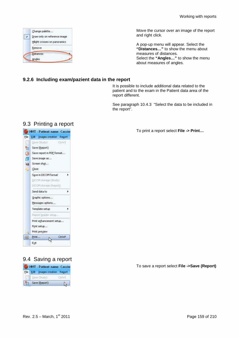
Working with reports
Rev. 2.5 – March, 1st 2011 Page 159 of 210
Move the cursor over an image of the reportand right click.
A pop-up menu will appear. Select the“ Distances… ” to show the menu aboutmeasures of distances.Select the “ Angles… ” to show the menuabout measures of angles.
9.2.6 Including exam/pazient data in the reportIt is possible to include additional data related to thepatient and to the exam in the Patient data area of thereport different.
See paragraph 10.4.3 “Select the data to be included inthe report”.
9.3 Printing a reportTo print a report select File -> Print…
9.4 Saving a reportTo save a report select File ->Save (Report)
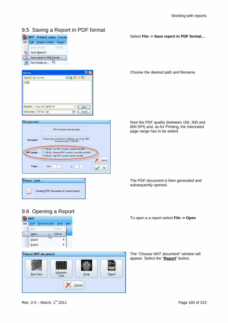
Working with reports
Rev. 2.5 – March, 1st 2011 Page 160 of 210
9.5 Saving a Report in PDF formatSelect File -> Save report in PDF format…
Choose the desired path and filename.
Now the PDF quality (between 150, 300 and600 DPI) and, as for Printing, the interestedpage range has to be setted.
The PDF document is then generated andsubsequently opened.
9.6 Opening a ReportTo open a a report select File -> Open
The “Choose NNT document” window willappear. Select the “Report ” button.
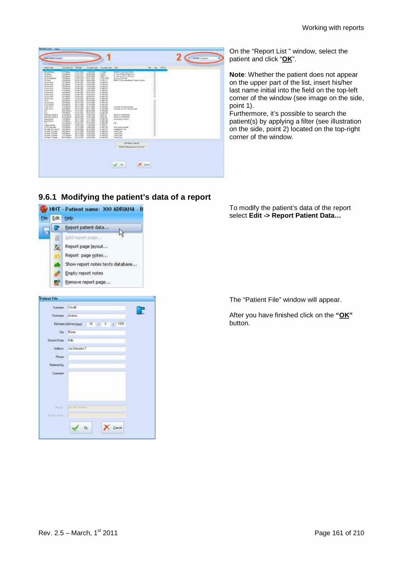
Working with reports
Rev. 2.5 – March, 1st 2011 Page 161 of 210
On the “Report List ” window, select thepatient and click “OK”.
Note : Whether the patient does not appearon the upper part of the list, insert his/herlast name initial into the field on the top-leftcorner of the window (see image on the side,point 1).Furthermore, it’s possible to search thepatient(s) by applying a filter (see illustrationon the side, point 2) located on the top-rightcorner of the window.
9.6.1 Modifying the patient’s data of a reportTo modify the patient’s data of the reportselect Edit -> Report Patient Data…
The “Patient File” window will appear.
After you have finished click on the “OK”button.
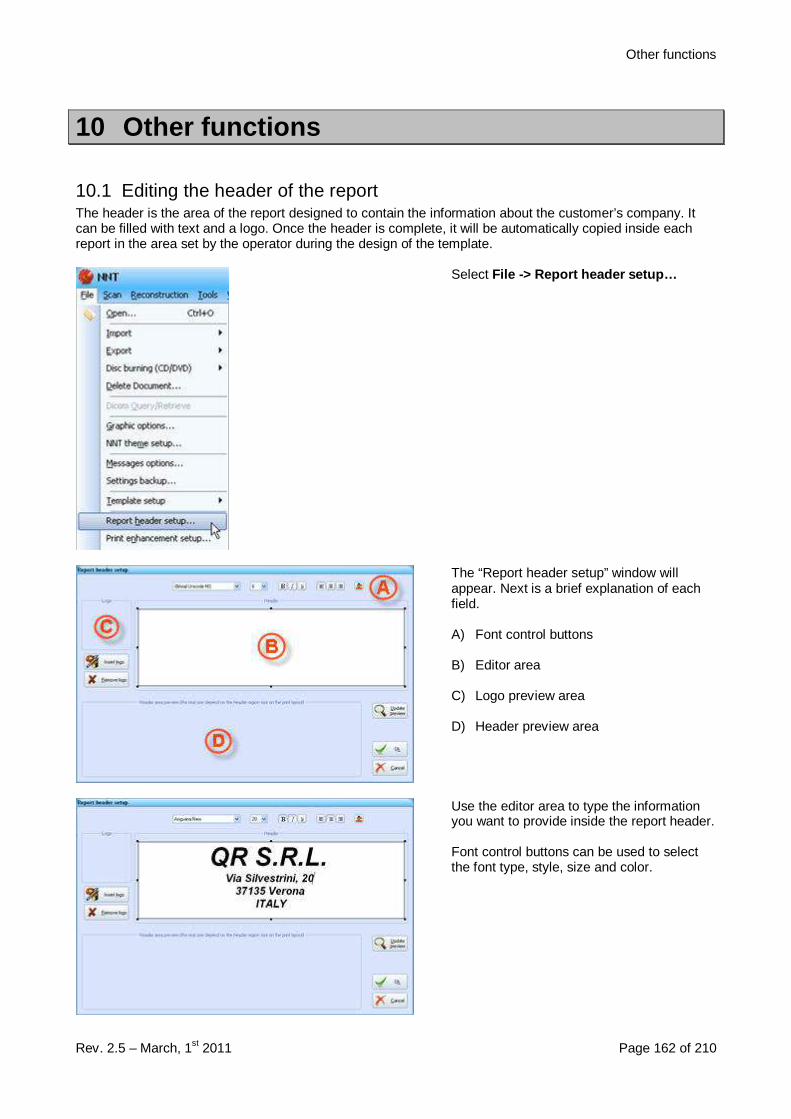
Other functions
Rev. 2.5 – March, 1st 2011 Page 162 of 210
10 Other functions
10.1 Editing the header of the reportThe header is the area of the report designed to contain the information about the customer’s company. Itcan be filled with text and a logo. Once the header is complete, it will be automatically copied inside eachreport in the area set by the operator during the design of the template.
Select File -> Report header setup…
The “Report header setup” window willappear. Next is a brief explanation of eachfield.
A) Font control buttons
B) Editor area
C) Logo preview area
D) Header preview area
Use the editor area to type the informationyou want to provide inside the report header.
Font control buttons can be used to selectthe font type, style, size and color.
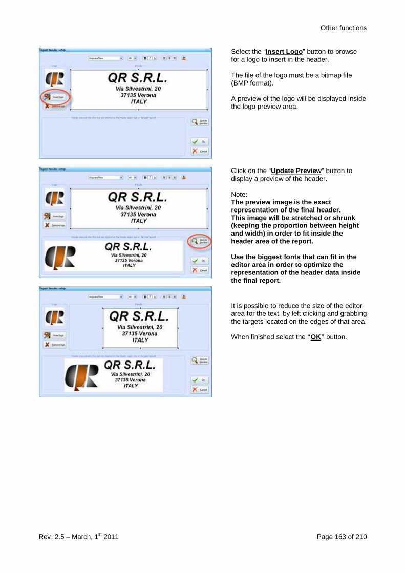
Other functions
Rev. 2.5 – March, 1st 2011 Page 163 of 210
Select the “Insert Logo ” button to browsefor a logo to insert in the header.
The file of the logo must be a bitmap file(BMP format).
A preview of the logo will be displayed insidethe logo preview area.
Click on the “Update Preview ” button todisplay a preview of the header.
Note:The preview image is the exactrepresentation of the final header.This image will be stretched or shrunk(keeping the proportion between heightand width) in order to fit inside theheader area of the report.
Use the biggest fonts that can fit in theeditor area in order to optimize therepresentation of the header data insidethe final report.
It is possible to reduce the size of the editorarea for the text, by left clicking and grabbingthe targets located on the edges of that area.
When finished select the “OK” button.
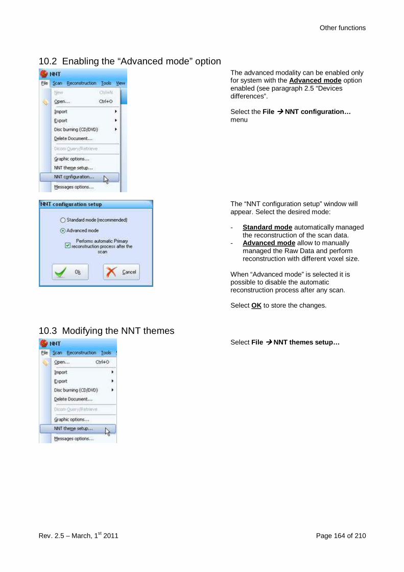
Other functions
Rev. 2.5 – March, 1st 2011 Page 164 of 210
10.2 Enabling the “Advanced mode” optionThe advanced modality can be enabled onlyfor system with the Advanced mode optionenabled (see paragraph 2.5 “Devicesdifferences”.
Select the File ���� NNT configuration…menu
The “NNT configuration setup” window willappear. Select the desired mode:
- Standard mode automatically managedthe reconstruction of the scan data.
- Advanced mode allow to manuallymanaged the Raw Data and performreconstruction with different voxel size.
When “Advanced mode” is selected it ispossible to disable the automaticreconstruction process after any scan.
Select OK to store the changes.
10.3 Modifying the NNT themesSelect File ���� NNT themes setup…
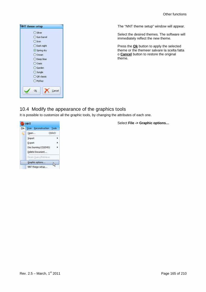
Other functions
Rev. 2.5 – March, 1st 2011 Page 165 of 210
The “NNT theme setup” window will appear.
Select the desired themes. The software willimmediately reflect the new theme.
Press the Ok button to apply the selectedtheme or the themeer salvare la scelta fattao Cancel button to restore the originaltheme.
10.4 Modify the appearance of the graphics toolsIt is possible to customize all the graphic tools, by changing the attributes of each one.
Select File -> Graphic options…

Other functions
Rev. 2.5 – March, 1st 2011 Page 166 of 210
This page should NOT be released to the final user
Rev n. Date1.0 2007/06/15 End of first version1.1 2007/08/06 Chapter 3.1: "warm up" is replaced by "conditioning"
Scan Pad "RX Shot" is replaced by "X-Ray Flash" along the manualChapter 2.4: added a new image representing the prescan padChapter 3 improvedChapter 4 is renamed into Chapter 3.4
1.2 2007/11/08 Reference to the software 2.11 release updatedRemoved any reference to the LITE versionAdded notes about the DICOM-images folder creation (11.3.1, 11.3.2 and 7.14)Removed restrictions about modifying a patient's data (9.2.3)Modified the figure about the study scout views and its description (7.3)Chapter 4: split into scan for patient and for dentureAdded paragraph 4.3Paragraph 7.5.3: added 1-3 panoramics number selection
2.0 2008/07/01 Paragraph 7.14 modified and its title is changed in “DICOM”Paragraphs 7.14.1, 7.14.2, 7.14.3, 7.14.4 addedChapters 11.1, 11.1.1, 11.1.2 adjournedChapters 11.3, 11.3.1, 11.3.2 adjournedChapter 9.6 addedChapters 11.5, 11.5.1, 11.5.2, 11.5.3, 11.5.4 addedChapter 14.2 changed
2.1 2009/02/15 Paragraphs 4.1.3 and 4.1.1 adjourned with new "NNT F.O.V. menu" imageChapter 10.6 addedParagraphs 11.5.1, 11.5.2, 11.5.3 and 11.5.4 adjournedChapters 13.1 and 13.2 deleted, chapter 13 modifiedChapters 6.4, 6.5 and 6.6 modified and 6.7 addedParagraphs 7.5.1, 7.5.2, 7.5.3, 7.5.6, 7.5.7, 7.14.1, 7.14.2 and 7.16 adjournedChapter 5.3 and 12.2 modifiedParagraph 9.1.3 adjournedChapter 2.3 modified
2.2 2009/10/24 Paragraph 5.4.1 modifiedParagraphs 7.5.1, 7.5.2, 7.5.3 modifiedChapter 13.3 added
2.3 2010/05/13 Paragraph 2.3.1 addedParagraphs 7.5.3 and 7.5.7 modified
2.4 2010/07/30 Manual completely adjourned for NNT version 3.0
Released and approved by the project manager:

Other functions
Rev. 2.5 – March, 1st 2011 Page 167 of 210
The “Graphics Options” window will appear.
On the left side of the dialog, the objects list(A) can be used to select the object tomodify.
The preview image (B) displays a preview ofthe selected object with its current attributes.
On the right side of the dialog box thegraphics attributes (C) are listed. Dependingon the selected object, attributes could behidden or grayed.Following is a list of the attributes:
• Font type : allows changing the texttype, style and size of the object.
• Font color : allows changing the textcolor of the object.
• BK font color : used to change thebackground color of the text of theobject.
• Transparent : set the background of thefont as transparent (no background)
• Overlay color : allows changing thecolor of the object.
• Ovl width : allows changing thethickness of the object.
Clicking on the “Save” button the newsettings will be applied.
Additional settings can be found for the lastfour objects listed on the left side of thewindow (“Single cross setup param”, “Crossseq. Setup param”, “Panoramic setupparam”, “3D setup param”).
The name and presence of these settingsvary depending on the selected object. Thefollowing are the fields that can be foundselecting the “Single cross setup param”object:
• Top-left corner on report: if selecteddraw the image parameters (D) (in thiscase only the thickness) on the top-leftcorner of the image (applicable only forthe report, not the study).
• Bottom-left corner on report: ifselected draw the image parameters (D)(in this case only the thickness) on thebottom-left corner of the image(applicable only for the report, not the
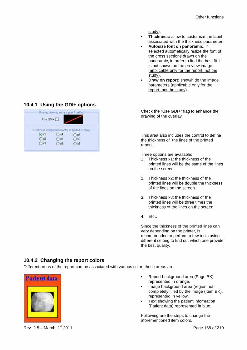
Other functions
Rev. 2.5 – March, 1st 2011 Page 168 of 210
study).• Thickness: allow to customize the label
associated with the thickness parameter.• Autosize font on panoramic: if
selected automatically resize the font ofthe cross sections drawn on thepanoramic, in order to find the best fit. Itis not shown on the preview image.(applicable only for the report, not thestudy).
• Draw on report: show/hide the imageparameters (applicable only for thereport, not the study).
10.4.1 Using the GDI+ optionsCheck the “Use GDI+” flag to enhance thedrawing of the overlay.
This area also includes the control to definethe thickness of the lines of the printedreport.
Three options are available:1. Thickness x1: the thickness of the
printed lines will be the same of the lineson the screen.
2. Thickness x2: the thickness of theprinted lines will be double the thicknessof the lines on the screen.
3. Thickness x3: the thickness of theprinted lines will be three times thethickness of the lines on the screen.
4. Etc…
Since the thickness of the printed lines canvary depending on the printer, isrecommended to perform a few tests usingdifferent setting to find out which one providethe best quality.
10.4.2 Changing the report colorsDifferent areas of the report can be associated with various color; these areas are:
• Report background area (Page BK)represented in orange.
• Image background area (region notcompletely filled by the image (Item BK),represented in yellow.
• Text showing the patient information(Patient data) represented in blue.
Following are the steps to change theaforementioned item colors.
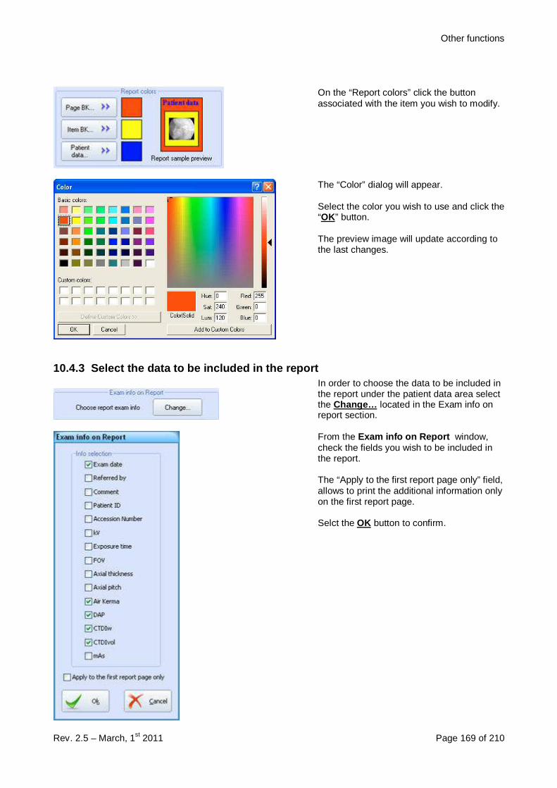
Other functions
Rev. 2.5 – March, 1st 2011 Page 169 of 210
On the “Report colors” click the buttonassociated with the item you wish to modify.
The “Color” dialog will appear.
Select the color you wish to use and click the“OK” button.
The preview image will update according tothe last changes.
10.4.3 Select the data to be included in the repor tIn order to choose the data to be included inthe report under the patient data area selectthe Change… located in the Exam info onreport section.
From the Exam info on Report window,check the fields you wish to be included inthe report.
The “Apply to the first report page only” field,allows to print the additional information onlyon the first report page.
Selct the OK button to confirm.
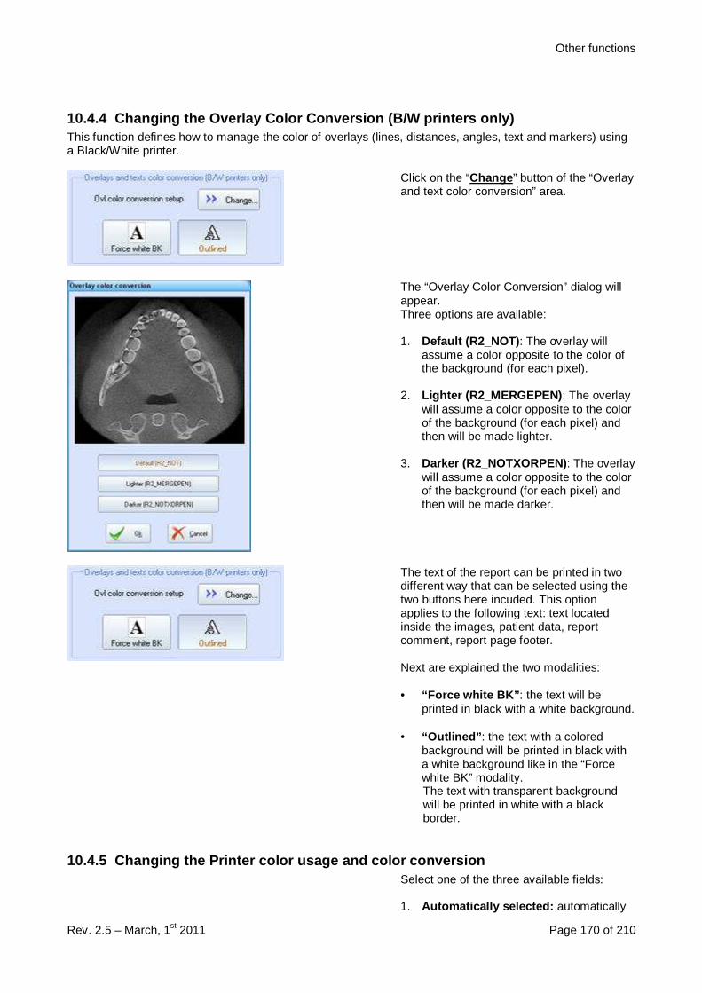
Other functions
Rev. 2.5 – March, 1st 2011 Page 170 of 210
10.4.4 Changing the Overlay Color Conversion (B/W printers only)This function defines how to manage the color of overlays (lines, distances, angles, text and markers) usinga Black/White printer.
Click on the “Change ” button of the “Overlayand text color conversion” area.
The “Overlay Color Conversion” dialog willappear.Three options are available:
1. Default (R2_NOT) : The overlay willassume a color opposite to the color ofthe background (for each pixel).
2. Lighter (R2_MERGEPEN) : The overlaywill assume a color opposite to the colorof the background (for each pixel) andthen will be made lighter.
3. Darker (R2_NOTXORPEN) : The overlaywill assume a color opposite to the colorof the background (for each pixel) andthen will be made darker.
The text of the report can be printed in twodifferent way that can be selected using thetwo buttons here incuded. This optionapplies to the following text: text locatedinside the images, patient data, reportcomment, report page footer.
Next are explained the two modalities:
• “Force white BK” : the text will beprinted in black with a white background.
• “Outlined” : the text with a coloredbackground will be printed in black witha white background like in the “Forcewhite BK” modality.The text with transparent backgroundwill be printed in white with a blackborder.
10.4.5 Changing the Printer color usage and color conversionSelect one of the three available fields:
1. Automatically selected: automatically

Other functions
Rev. 2.5 – March, 1st 2011 Page 171 of 210
recognize the type of printer and how tomanage colors.
2. Force colors: print objects and overlaysalways using color (or variations ofgray), for any printer.
3. Force Monochrome: print objects andoverlays always using black and white(reversing overlay background system),for any printer.
10.4.6 Print OptimizeThe Optimized print process optionlocated on the Printing section, whenenabled, use a slightly slow process thatimproves the compatibility with differentprintersr.
10.4.7 Apply a ruler on the imagesIt is possible to insert a ruler on the right side of scout, axials, transaxials (single and sequence) andpanoramics images. Once the ruler is enabled it will be applied to all the aforementioned images. Next arethe steps to follow:
On the “Image ruler” area select the “Setup ”button.
The “ Image ruler setup ” window willappear. Select the “Enable ” button.
The following options will became enabled:
• Ruler color: allows to choose the colourof the ruler.
• Ruler step: set the step between twotags (1 or 5 mm).
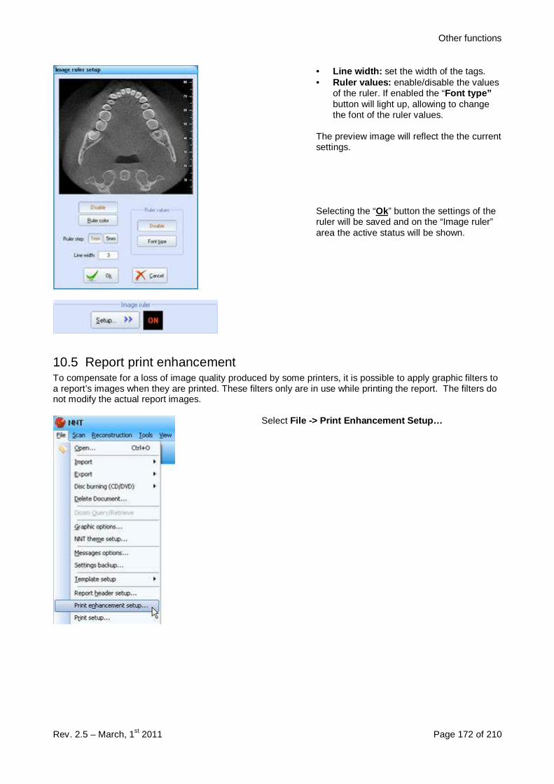
Other functions
Rev. 2.5 – March, 1st 2011 Page 172 of 210
• Line width: set the width of the tags.• Ruler values: enable/disable the values
of the ruler. If enabled the “Font type”button will light up, allowing to changethe font of the ruler values.
The preview image will reflect the the currentsettings.
Selecting the “Ok” button the settings of theruler will be saved and on the “Image ruler”area the active status will be shown.
10.5 Report print enhancementTo compensate for a loss of image quality produced by some printers, it is possible to apply graphic filters toa report’s images when they are printed. These filters only are in use while printing the report. The filters donot modify the actual report images.
Select File -> Print Enhancement Setup…

Other functions
Rev. 2.5 – March, 1st 2011 Page 173 of 210
The “Print Enhancement Filter Setup ” window willappear. Left click on the drop down lists to select a filter.
Five filters are available:1) None (no filter applied).
2) Soften: Low-pass filter. Smoothes the edges ofthe images and reduces noise.
3) Sharpen: High-pass filter. Sharpens the edges ofthe image.
4) Enhance Edge: Enhances the edges of theimage.
5) Adaptive: Analyzes the image, and for each pixelchooses a filter depending on the pixelinformation. It will consider both the noise(reducing it) and the real information(emphasizing it.)
It is strongly recommended users, to print a report thenchange the filter and print the same report once again.The results depend upon the printer. The results of theseadjustments are purely subjective. After making changesto the settings, click on “OK”. The settings will be used forall the following print jobs.
10.6 3M printers & DICOMIf a 3M printer (printers using a 3M interface card) or a DICOM printer is used, it will require uniqueconsiderations in its setup.The setup of the printer is performed at a service level by the technician. To display the configuration of theprinter follow the next steps.
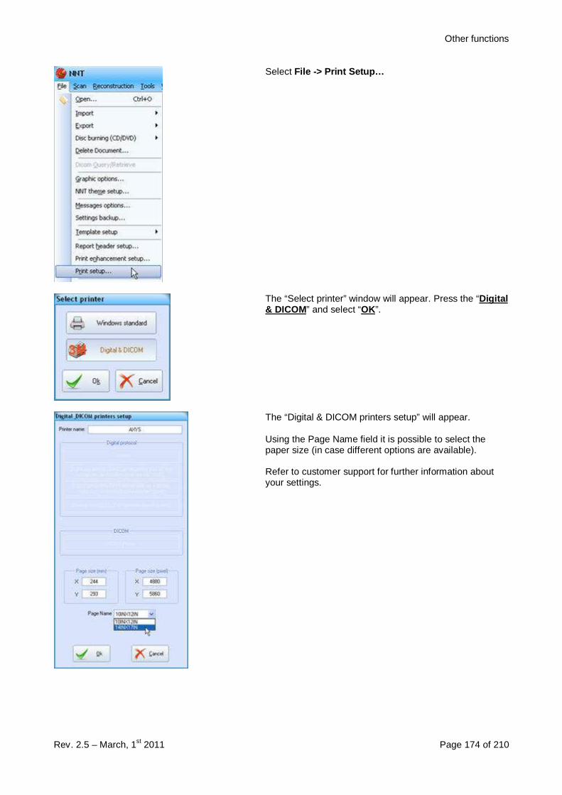
Other functions
Rev. 2.5 – March, 1st 2011 Page 174 of 210
Select File -> Print Setup…
The “Select printer” window will appear. Press the “Digital& DICOM” and select “OK”.
The “Digital & DICOM printers setup” will appear.
Using the Page Name field it is possible to select thepaper size (in case different options are available).
Refer to customer support for further information aboutyour settings.

Other functions
Rev. 2.5 – March, 1st 2011 Page 175 of 210
10.7 System files backupThe backup of the system files, consists in an automatic backup of a few files containing data regarding thescanner configuration (only for the main workstation), software customized user settings and other softwareconfiguration files.It is suggested to perform a backup of this files at least once a week. Next are the steps to perform thebackup:
1. From the main menu bar select File -> SettingsBackup.
2. The “Import/Export path setup” window will appear.The “Current path” field define the directory where thebackup of the system file will be stored.
Select the “Change path” button to change thecurrent path.
Use the “New Folder” field to type the name of a newfolder. Select the “Add Folder” button to add the newfolder to the current path.
3. Once done, select the “Go on”.
4. The backup process will start in background. At theend a message will appear informing that the processis finished.
NOTE: If error messages appear during the backupprocess, ignore them. These messages refer to files thatare installed only on the main workstation(scannerconsole).
10.8 Use of the VDDS protocolIn the NNT software only one functionality of the VDDS protocol has been implemented: the patient dataimport.To active this function it is necessary, after a correct NNT installation, to launch the NNT_VDDS.exeprogram that is in the same directory than NNT.exe.

Other functions
Rev. 2.5 – March, 1st 2011 Page 176 of 210
To permit other VDDS programs to launch NNT with preloaded patient data the Registration is needed;when it has to return at the previous condition (VDDS disabled) the Unregistration button has to be clicked.Now, after the assuring that NNT is not running, using any VDDS patient managing program it is possible tochoose a patient and to launch, directly from there, NNT.
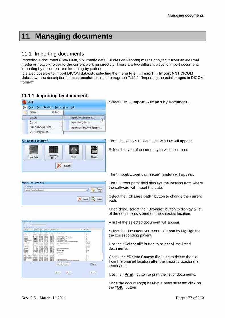
Managing documents
Rev. 2.5 – March, 1st 2011 Page 177 of 210
11 Managing documents
11.1 Importing documentsImporting a document (Raw Data, Volumetric data, Studies or Reports) means copying it from an externalmedia or network folder to the current working directory. There are two different ways to import document:importing by document and importing by patient.It is also possible to import DICOM datasets selecting the menu File →→→→ Import →→→→ Import NNT DICOMdataset… , the description of this procedure is in the paragraph 7.14.2 “Importing the axial images in DICOMformat”
11.1.1 Importing by documentSelect File →→→→ Import →→→→ Import by Document…
The “Choose NNT Document” window will appear.
Select the type of document you wish to import.
The “Import/Export path setup” window will appear.
The “Current path” field displays the location from wherethe software will import the data.
Select the “Change path” button to change the currentpath.
Once done, select the “Browse” button to display a listof the documents stored on the selected location.
A list of the selected document will appear.
Select the document you want to import by highlightingthe corresponding patient.
Use the “Select all” button to select all the listeddocuments.
Check the “Delete Source file” flag to delete the filefrom the original location after the import procedure isterminated.
Use the “Print” button to print the list of documents.
Once the document(s) has/have been selected click onthe “OK” button
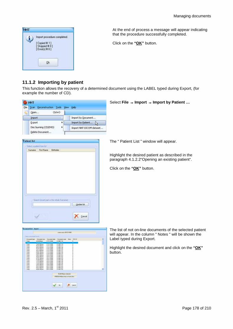
Managing documents
Rev. 2.5 – March, 1st 2011 Page 178 of 210
At the end of process a message will appear indicatingthat the procedure successfully completed.
Click on the “OK” button.
11.1.2 Importing by patientThis function allows the recovery of a determined document using the LABEL typed during Export, (forexample the number of CD).
Select File →→→→ Import →→→→ Import by Patient …
The “ Patient List ” window will appear.
Highlight the desired patient as described in theparagraph 4.1.2.2“Opening an existing patient“.
Click on the “OK” button.
The list of not on-line documents of the selected patientwill appear. In the column " Notes " will be shown theLabel typed during Export.
Highlight the desired document and click on the “OK”button.
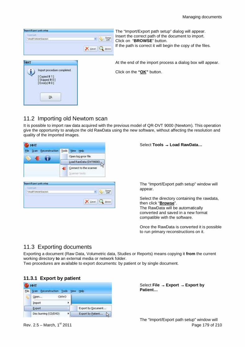
Managing documents
Rev. 2.5 – March, 1st 2011 Page 179 of 210
The “Import/Export path setup” dialog will appear.Insert the correct path of the document to import.Click on “BROWSE” button.If the path is correct it will begin the copy of the files.
At the end of the import process a dialog box will appear.
Click on the “OK” button.
11.2 Importing old Newtom scanIt is possible to import raw data acquired with the previous model of QR-DVT 9000 (Newtom). This operationgive the opportunity to analyze the old RawData using the new software, without affecting the resolution andquality of the imported images.
Select Tools →→→→ Load RawData…
The “Import/Export path setup” window willappear.
Select the directory containing the rawdata,then click “Browse ”.The RawData will be automaticallyconverted and saved in a new formatcompatible with the software.
Once the RawData is converted it is possibleto run primary reconstructions on it.
11.3 Exporting documentsExporting a document (Raw Data, Volumetric data, Studies or Reports) means copying it from the currentworking directory to an external media or network folder.Two procedures are available to export documents: by patient or by single document.
11.3.1 Export by patientSelect File →→→→ Export →→→→ Export byPatient…
The “Import/Export path setup” window will

Managing documents
Rev. 2.5 – March, 1st 2011 Page 180 of 210
appear.
The “Current path” field displays the locationwhere the software will export the data.
Select the “Change path” button to changethe current path.
Use the “New Folder” field to type the nameof a new folder. Select the “Add Folder”button to add the new folder to the currentpath.
Once done, select the “Go on”
NOTE: exporting RawData, Volumetric Data,Studies and Reports, in the added folderanother one will be created, named..\Surname_Name_AAAAMMGGOfBirth.Such folder will store the DICOM images.
The “Patient List” window will appear.
To select a patient type the initial, part or theentire surname inside the “Search” field,then click on the “Update list” button.
The “Patient list” window will be updateddisplaying all the patients that match thecriteria used for the search.
Highlight the patient to be exported andselect the “OK” button.
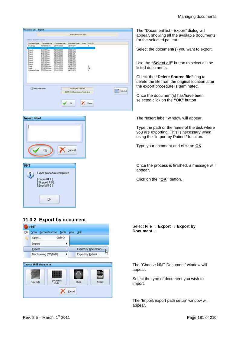
Managing documents
Rev. 2.5 – March, 1st 2011 Page 181 of 210
The “Document list - Export” dialog willappear, showing all the available documentsfor the selected patient.
Select the document(s) you want to export.
Use the “Select all” button to select all thelisted documents.
Check the “Delete Source file” flag todelete the file from the original location afterthe export procedure is terminated.
Once the document(s) has/have beenselected click on the “OK” button
The “Insert label” window will appear.
Type the path or the name of the disk whereyou are exporting. This is necessary whenusing the “Import by Patient” function.
Type your comment and click on OK.
Once the process is finished, a message willappear.
Click on the “OK” button.
11.3.2 Export by documentSelect File →→→→ Export →→→→ Export byDocument…
The “Choose NNT Document” window willappear.
Select the type of document you wish toimport.
The “Import/Export path setup” window willappear.

Managing documents
Rev. 2.5 – March, 1st 2011 Page 182 of 210
The “Current path” field displays the locationwhere the software will export the data.
Select the “Change path” button to changethe current path.
Use the “New Folder” field to type the name ofa new folder. Select the “Add Folder” buttonto add the new folder to the current path.
Once done, select the “Go on”
NOTE: exporting RawData, Volumetric Data,Studies and Reports, in the added folderanother one will be created, named..\Surname_Name_AAAAMMGGOfBirth. Suchfolder will store the DICOM images.
The selected document export list dialog willappear, showing all the available patients forthe selected document.
Select the patient(s) you want to export.
Use the “Select all” button to select all thelisted patients.
Check the “Delete Source file” flag to deletethe file from the original location after theexport procedure is terminated.
Once the document(s) has/have been selectedclick on the “OK” button
The “Insert label” window will appear.
Type a distinguishing comment related to thisexport process. This identifies the differentexport operations completed.
Type your comment and click on OK.
Once the process is finished, a message willappear.
Click on the “OK” button.
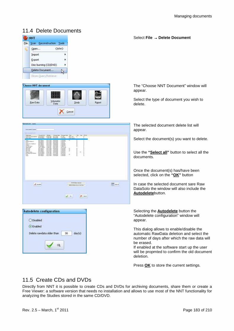
Managing documents
Rev. 2.5 – March, 1st 2011 Page 183 of 210
11.4 Delete DocumentsSelect File →→→→ Delete Document
The “Choose NNT Document” window willappear.
Select the type of document you wish todelete.
The selected document delete list willappear.
Select the document(s) you want to delete.
Use the “Select all” button to select all thedocuments.
Once the document(s) has/have beenselected, click on the “OK” button
In case the selected document sare RawDataSolo the window will also include theAutodelete button.
Selecting the Autodelete button the“Autodelete configuration” window willappear.
This dialog allows to enable/disable theautomatic RawData deletion and select thenumber of days after which the raw data willbe erased.If enabled at the software start up the userwill be propmted to confirm the old documentdeletion.
Press OK to store the current settings.
11.5 Create CDs and DVDsDirectly from NNT it is possible to create CDs and DVDs for archiving documents, share them or create aFree Viewer: a software version that needs no installation and allows to use most of the NNT functionality foranalyzing the Studies stored in the same CD/DVD.
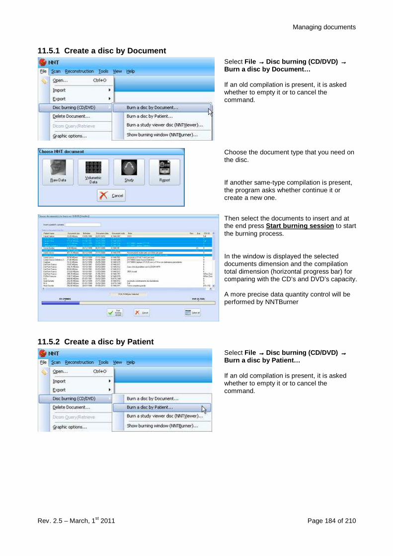
Managing documents
Rev. 2.5 – March, 1st 2011 Page 184 of 210
11.5.1 Create a disc by DocumentSelect File →→→→ Disc burning (CD/DVD) →→→→Burn a disc by Document…
If an old compilation is present, it is askedwhether to empty it or to cancel thecommand.
Choose the document type that you need onthe disc.
If another same-type compilation is present,the program asks whether continue it orcreate a new one.
Then select the documents to insert and atthe end press Start burning session to startthe burning process.
In the window is displayed the selecteddocuments dimension and the compilationtotal dimension (horizontal progress bar) forcomparing with the CD’s and DVD’s capacity.
A more precise data quantity control will beperformed by NNTBurner
11.5.2 Create a disc by PatientSelect File →→→→ Disc burning (CD/DVD) →→→→Burn a disc by Patient…
If an old compilation is present, it is askedwhether to empty it or to cancel thecommand.
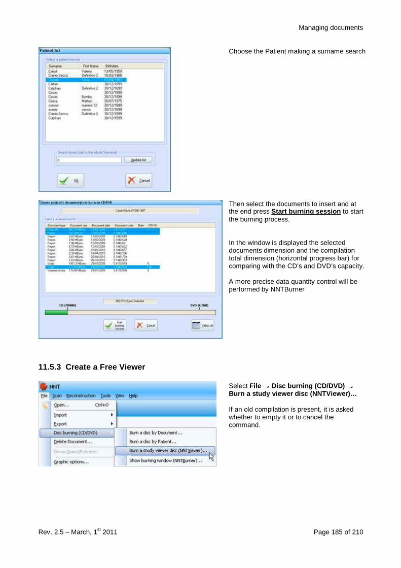
Managing documents
Rev. 2.5 – March, 1st 2011 Page 185 of 210
Choose the Patient making a surname search
Then select the documents to insert and atthe end press Start burning session to startthe burning process.
In the window is displayed the selecteddocuments dimension and the compilationtotal dimension (horizontal progress bar) forcomparing with the CD’s and DVD’s capacity.
A more precise data quantity control will beperformed by NNTBurner
11.5.3 Create a Free Viewer
Select File →→→→ Disc burning (CD/DVD) →→→→Burn a study viewer disc (NNTViewer)…
If an old compilation is present, it is askedwhether to empty it or to cancel thecommand.
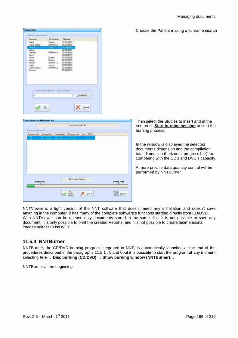
Managing documents
Rev. 2.5 – March, 1st 2011 Page 186 of 210
Choose the Patient making a surname search
Then select the Studies to insert and at theend press Start burning session to start theburning process.
In the window is displayed the selecteddocuments dimension and the compilationtotal dimension (horizontal progress bar) forcomparing with the CD’s and DVD’s capacity.
A more precise data quantity control will beperformed by NNTBurner
NNTViewer is a light version of the NNT software that doesn’t need any installation and doesn’t saveanything in the computer, it has many of the complete software’s functions starting directly from CD/DVD.With NNTViewer can be opened only documents stored in the same disc, it is not possible to save anydocument, it is only possible to print the created Reports, and it is not possible to create tridimensionalimages neither CDs/DVDs.
11.5.4 NNTBurnerNNTBurner, the CD/DVD burning program integrated in NNT, is automatically launched at the end of theprocedures described in the paragraphs 11.5.1 , 0 and 0but it is possible to start the program at any momentselecting File →→→→ Disc burning (CD/DVD) →→→→ Show burning window (NNTBurner)…
NNTBurner at the beginning:
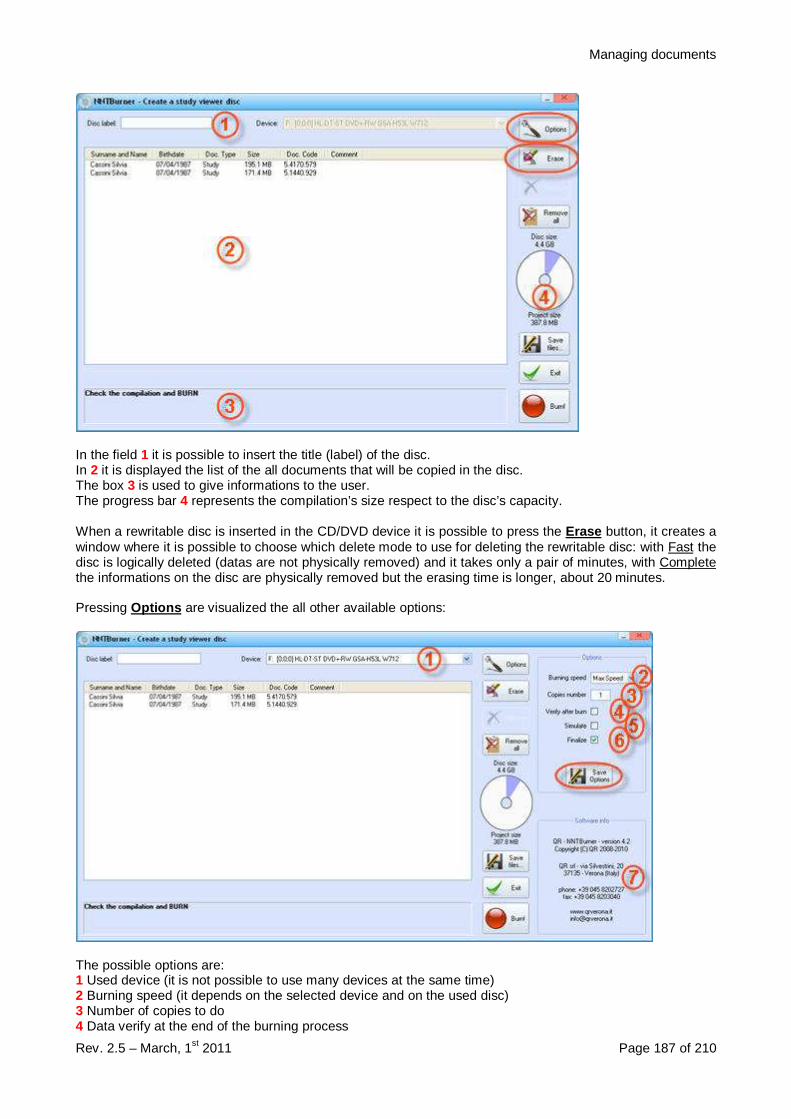
Managing documents
Rev. 2.5 – March, 1st 2011 Page 187 of 210
In the field 1 it is possible to insert the title (label) of the disc.In 2 it is displayed the list of the all documents that will be copied in the disc.The box 3 is used to give informations to the user.The progress bar 4 represents the compilation’s size respect to the disc’s capacity.
When a rewritable disc is inserted in the CD/DVD device it is possible to press the Erase button, it creates awindow where it is possible to choose which delete mode to use for deleting the rewritable disc: with Fast thedisc is logically deleted (datas are not physically removed) and it takes only a pair of minutes, with Completethe informations on the disc are physically removed but the erasing time is longer, about 20 minutes.
Pressing Options are visualized the all other available options:
The possible options are:1 Used device (it is not possible to use many devices at the same time)2 Burning speed (it depends on the selected device and on the used disc)3 Number of copies to do4 Data verify at the end of the burning process
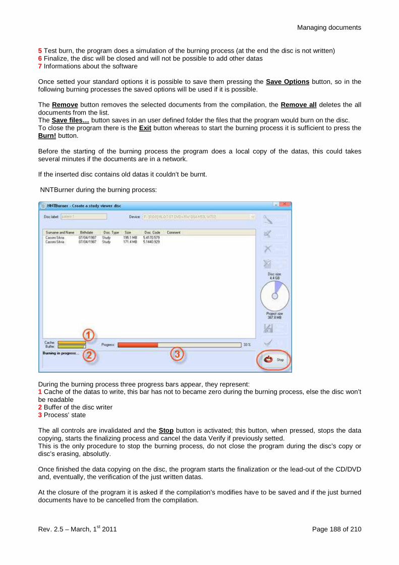
Managing documents
Rev. 2.5 – March, 1st 2011 Page 188 of 210
5 Test burn, the program does a simulation of the burning process (at the end the disc is not written)6 Finalize, the disc will be closed and will not be possible to add other datas7 Informations about the software
Once setted your standard options it is possible to save them pressing the Save Options button, so in thefollowing burning processes the saved options will be used if it is possible.
The Remove button removes the selected documents from the compilation, the Remove all deletes the alldocuments from the list.The Save files… button saves in an user defined folder the files that the program would burn on the disc.To close the program there is the Exit button whereas to start the burning process it is sufficient to press theBurn! button.
Before the starting of the burning process the program does a local copy of the datas, this could takesseveral minutes if the documents are in a network.
If the inserted disc contains old datas it couldn’t be burnt.
NNTBurner during the burning process:
During the burning process three progress bars appear, they represent:1 Cache of the datas to write, this bar has not to became zero during the burning process, else the disc won’tbe readable2 Buffer of the disc writer3 Process’ state
The all controls are invalidated and the Stop button is activated; this button, when pressed, stops the datacopying, starts the finalizing process and cancel the data Verify if previously setted.This is the only procedure to stop the burning process, do not close the program during the disc’s copy ordisc’s erasing, absolutly.
Once finished the data copying on the disc, the program starts the finalization or the lead-out of the CD/DVDand, eventually, the verification of the just written datas.
At the closure of the program it is asked if the compilation’s modifies have to be saved and if the just burneddocuments have to be cancelled from the compilation.
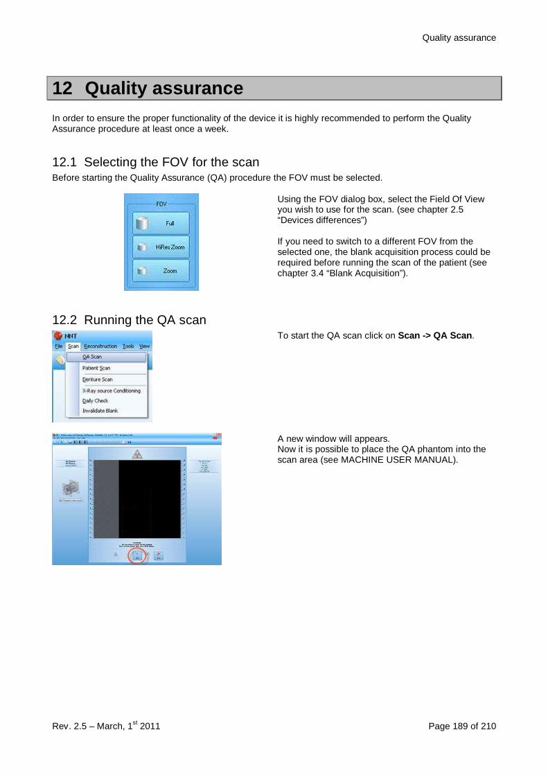
Quality assurance
Rev. 2.5 – March, 1st 2011 Page 189 of 210
12 Quality assuranceIn order to ensure the proper functionality of the device it is highly recommended to perform the QualityAssurance procedure at least once a week.
12.1 Selecting the FOV for the scanBefore starting the Quality Assurance (QA) procedure the FOV must be selected.
Using the FOV dialog box, select the Field Of Viewyou wish to use for the scan. (see chapter 2.5“Devices differences”)
If you need to switch to a different FOV from theselected one, the blank acquisition process could berequired before running the scan of the patient (seechapter 3.4 “Blank Acquisition”).
12.2 Running the QA scanTo start the QA scan click on Scan -> QA Scan .
A new window will appears.Now it is possible to place the QA phantom into thescan area (see MACHINE USER MANUAL).
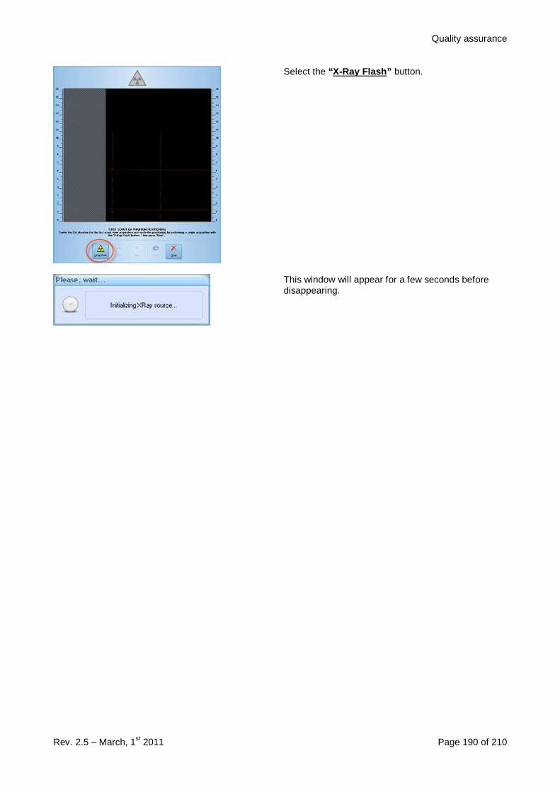
Quality assurance
Rev. 2.5 – March, 1st 2011 Page 190 of 210
Select the “ X-Ray Flash ” button.
This window will appear for a few seconds beforedisappearing.
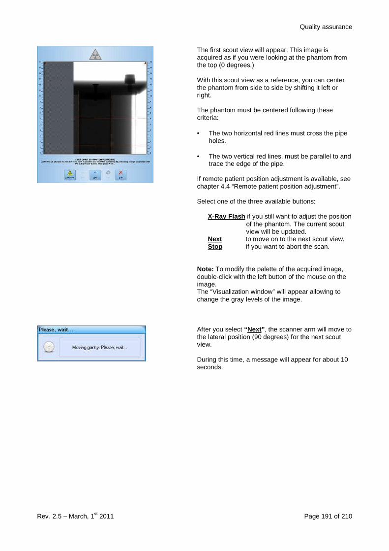
Quality assurance
Rev. 2.5 – March, 1st 2011 Page 191 of 210
The first scout view will appear. This image isacquired as if you were looking at the phantom fromthe top (0 degrees.)
With this scout view as a reference, you can centerthe phantom from side to side by shifting it left orright.
The phantom must be centered following thesecriteria:
• The two horizontal red lines must cross the pipeholes.
• The two vertical red lines, must be parallel to andtrace the edge of the pipe.
If remote patient position adjustment is available, seechapter 4.4 “Remote patient position adjustment”.
Select one of the three available buttons:
X-Ray Flash if you still want to adjust the positionof the phantom. The current scoutview will be updated.
Next to move on to the next scout view.Stop if you want to abort the scan.
Note: To modify the palette of the acquired image,double-click with the left button of the mouse on theimage.The “Visualization window” will appear allowing tochange the gray levels of the image.
After you select “Next” , the scanner arm will move tothe lateral position (90 degrees) for the next scoutview.
During this time, a message will appear for about 10seconds.
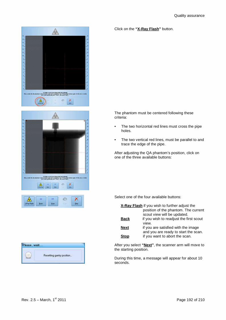
Quality assurance
Rev. 2.5 – March, 1st 2011 Page 192 of 210
Click on the “X-Ray Flash” button.
The phantom must be centered following thesecriteria:
• The two horizontal red lines must cross the pipeholes.
• The two vertical red lines, must be parallel to andtrace the edge of the pipe.
After adjusting the QA phantom’s position, click onone of the three available buttons:
Select one of the four available buttons:
X-Ray Flash if you wish to further adjust theposition of the phantom. The currentscout view will be updated.
Back if you wish to readjust the first scoutview.
Next if you are satisfied with the imageand you are ready to start the scan.
Stop if you want to abort the scan.
After you select “Next” , the scanner arm will move tothe starting position.
During this time, a message will appear for about 10seconds.
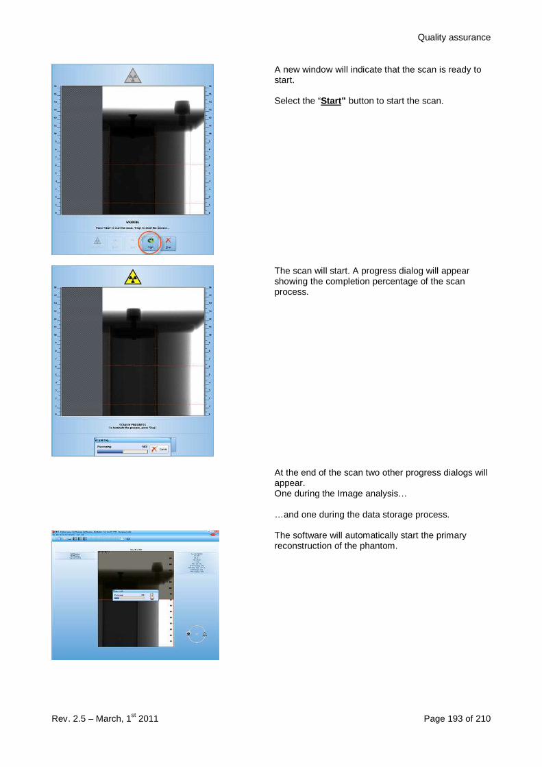
Quality assurance
Rev. 2.5 – March, 1st 2011 Page 193 of 210
A new window will indicate that the scan is ready tostart.
Select the “Start” button to start the scan.
The scan will start. A progress dialog will appearshowing the completion percentage of the scanprocess.
At the end of the scan two other progress dialogs willappear.One during the Image analysis…
…and one during the data storage process.
The software will automatically start the primaryreconstruction of the phantom.
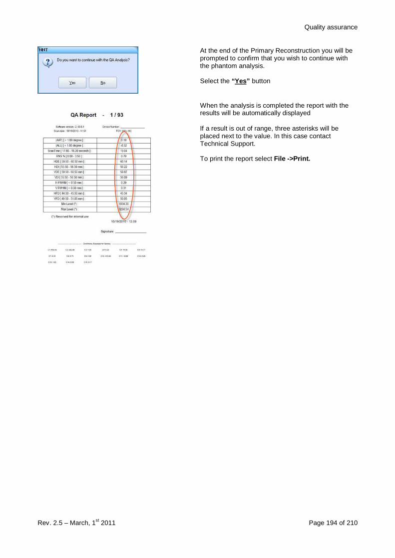
Quality assurance
Rev. 2.5 – March, 1st 2011 Page 194 of 210
At the end of the Primary Reconstruction you will beprompted to confirm that you wish to continue withthe phantom analysis.
Select the “Yes” button
When the analysis is completed the report with theresults will be automatically displayed
If a result is out of range, three asterisks will beplaced next to the value. In this case contactTechnical Support.
To print the report select File ->Print.

Quality assurance
Rev. 2.5 – March, 1st 2011 Page 195 of 210
The following table illustrates the meaning of each analysis result.
Abbreviation Name Description
AAP Phantom’s angle on theFirst scout view
Inclination angle of the phantom’s axis of symmetry in the First scoutview (0°)
AAL Phantom’s angle on theSecond scout view
Inclination angle of the phantom’s axis of symmetry in the Secondscout view (90°)
ScanTime Scan Time Scan time in seconds
RNS% Noise per cent Noise per cent on the phantom’s central axial image expressed asstandard deviation of the density values as to their average value inan area in the middle of the image (in correspondence of the water).
HDE External HorizontalDiameter
External diameter of the aluminum cylinder along the x-axis in thecentral axial image
HDI Internal HorizontalDiameter
Internal diameter of the aluminum cylinder along the x-axis in thecentral axial image
VDE External VerticalDiameter
External diameter of the aluminum cylinder along the y-axis in thecentral axial image
VDI Internal VerticalDiameter
Internal diameter of the aluminum cylinder along the y-axis in thecentral axial image
H FWHM Full Width HalfMaximum horizontal
Spatial resolution (millimeters) on the horizontal diameter of thecentral axial image
V FWHM Full Width HalfMaximum vertical
Spatial resolution (millimeters) on the vertical diameter of the centralaxial image
HFD Horizontal Distanceamong holes
Average horizontal distance among the holes of the cylinder on thepanoramic image
VFD Vertical Distanceamong holes
Average vertical distance among the holes of the cylinder on thepanoramic image
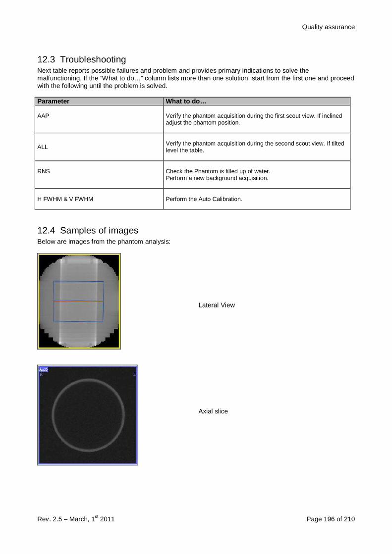
Quality assurance
Rev. 2.5 – March, 1st 2011 Page 196 of 210
12.3 TroubleshootingNext table reports possible failures and problem and provides primary indications to solve themalfunctioning. If the “What to do…” column lists more than one solution, start from the first one and proceedwith the following until the problem is solved.
Parameter What to do…
AAP Verify the phantom acquisition during the first scout view. If inclinedadjust the phantom position.
ALLVerify the phantom acquisition during the second scout view. If tiltedlevel the table.
RNS Check the Phantom is filled up of water.Perform a new background acquisition.
H FWHM & V FWHM Perform the Auto Calibration.
12.4 Samples of imagesBelow are images from the phantom analysis:
Lateral View
Axial slice
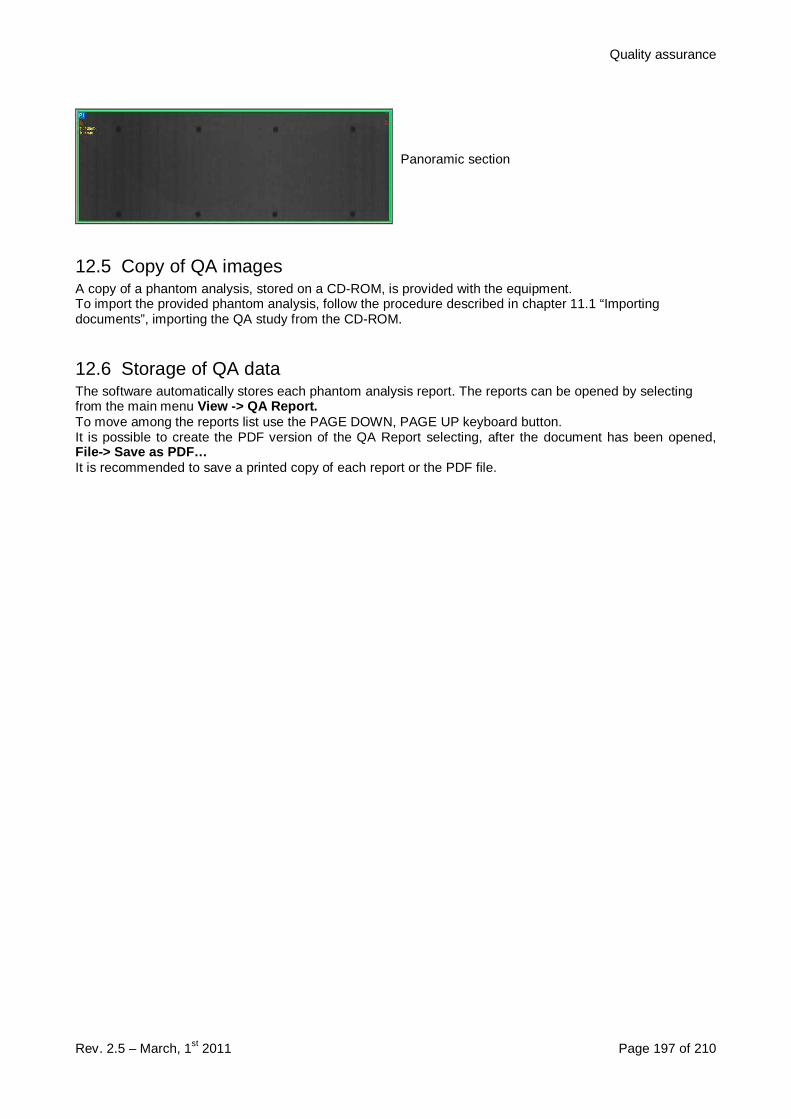
Quality assurance
Rev. 2.5 – March, 1st 2011 Page 197 of 210
Panoramic section
12.5 Copy of QA imagesA copy of a phantom analysis, stored on a CD-ROM, is provided with the equipment.To import the provided phantom analysis, follow the procedure described in chapter 11.1 “Importingdocuments”, importing the QA study from the CD-ROM.
12.6 Storage of QA dataThe software automatically stores each phantom analysis report. The reports can be opened by selectingfrom the main menu View -> QA Report.To move among the reports list use the PAGE DOWN, PAGE UP keyboard button.It is possible to create the PDF version of the QA Report selecting, after the document has been opened,File-> Save as PDF…It is recommended to save a printed copy of each report or the PDF file.
Troubleshooting
Rev. 2.5 – March, 1st 2011 Page 198 of 210
13 Troubleshooting
13.1 Errors GuideFor simplifying the solution of eventual problems that could appear in NNT it was created an attached document thatcollect the all possible software’s errors code, the description of the occurred error and its possible solutions.
This document is called Errors Guide and it is a part of the setup CD.
This is the first page:
13.2 Log ErrorAny occurred error is saved in a Log file and the errors history can be seen selecting, at the software start,Tools->Open log error file .The Log Error can be printed or saved in PDF format, in this last case additional informations about thecomputer are inserted in the file.

Troubleshooting
Rev. 2.5 – March, 1st 2011 Page 199 of 210
13.3 Remote support
To have remote support on yourcomputer, after ensuring that it isconnected on a network that allow internetaccess, select from the starting menuHelp����NNT Remote Support…
The NNT Remote Support will belauched.
Do not close the program andcommunicate to Service the ID and thePassword that you can read in theappropriate fields.
If some connection problems happenedthis screenshot would appear.
In this situation contact your networkadministrator and ask for NNT RemoteSupport (TeamViewer) to work properly.
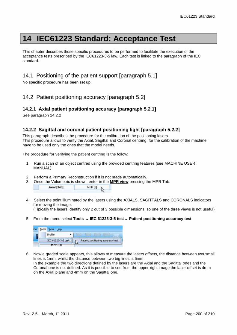
IEC61223 Standard
Rev. 2.5 – March, 1st 2011 Page 200 of 210
14 IEC61223 Standard: Acceptance TestThis chapter describes those specific procedures to be performed to facilitate the execution of theacceptance tests prescribed by the IEC61223-3-5 law. Each test is linked to the paragraph of the IECstandard.
14.1 Positioning of the patient support [paragraph 5.1]No specific procedure has been set up.
14.2 Patient positioning accuracy [paragraph 5.2]
14.2.1 Axial patient positioning accuracy [paragra ph 5.2.1]See paragraph 14.2.2
14.2.2 Sagittal and coronal patient positioning li ght [paragraph 5.2.2]This paragraph describes the procedure for the calibration of the positioning lasers.This procedure allows to verify the Axial, Sagittal and Coronal centring; for the calibration of the machinehave to be used only the ones that the model needs.
The procedure for verifying the patient centring is the follow:
1. Run a scan of an object centred using the provided centring features (see MACHINE USERMANUAL).
2. Perform a Primary Reconstruction if it is not made automatically.3. Once the Volumetric is shown, enter in the MPR view pressing the MPR Tab.
4. Select the point illuminated by the lasers using the AXIALS, SAGITTALS and CORONALS indicatorsfor moving the image.(Tipically the lasers identify only 2 out of 3 possible dimensions, so one of the three views is not useful)
5. From the menu select Tools →→→→ IEC 61223-3-5 test →→→→ Patient positioning accuracy test
6. Now a graded scale appears, this allows to measure the lasers offsets, the distance between two smalllines is 1mm, whilst the distance between two big lines is 5mm.In the example the two directions defined by the lasers are the Axial and the Sagittal ones and theCoronal one is not defined. As it is possible to see from the upper-right image the laser offset is 4mmon the Axial plane and 4mm on the Sagittal one.
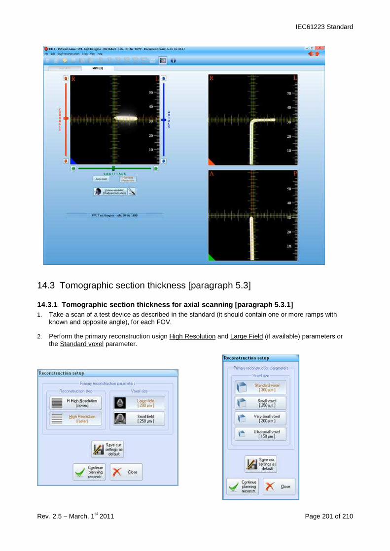
IEC61223 Standard
Rev. 2.5 – March, 1st 2011 Page 201 of 210
14.3 Tomographic section thickness [paragraph 5.3]
14.3.1 Tomographic section thickness for axial sca nning [paragraph 5.3.1]1. Take a scan of a test device as described in the standard (it should contain one or more ramps with
known and opposite angle), for each FOV.
2. Perform the primary reconstruction usign High Resolution and Large Field (if available) parameters orthe Standard voxel parameter.

IEC61223 Standard
Rev. 2.5 – March, 1st 2011 Page 202 of 210
3. At the end of the reconstruction, select [Study Reconstruction] from the [Study Reconstruction] menu.The slice thickness should be fixed to 0.5, 1 and 5mm.
4. Align the inclination of the Roi to the test device (in standard CT has to be done at the scanning time, inNewtom can be done at the reconstruction time).
5. For each slice thickness, open the study and visualize axial images. Set the single axial mode andbrowse the images till the ramp will appear.
6. Select [IEC 61223-3-5 test] and then [Tomographic Slice thickness test] from the [Tools] menu.
7. Trace a line (press the left button of the mouse, move it and at the end press the left button again), aslongitudinal as possible, over the bar that has to be analyzed (see following picture).

IEC61223 Standard
Rev. 2.5 – March, 1st 2011 Page 203 of 210
8. Appear the window of the density profile. Move the mouse inside the graph until a half of backgrounddisappear (a half of the image is white and a half is black). Press the left button of the mouse to fix thebackground value.
9. Move the mouse inside the graph and fix (with the left button of the mouse) the new line to the maximumgray level.
10. The software will calculate the FWHM value, showed in the square under the graph. Multiply themeasured FWHM by the tangent ramp-scan plane to obtain the slice thickness.
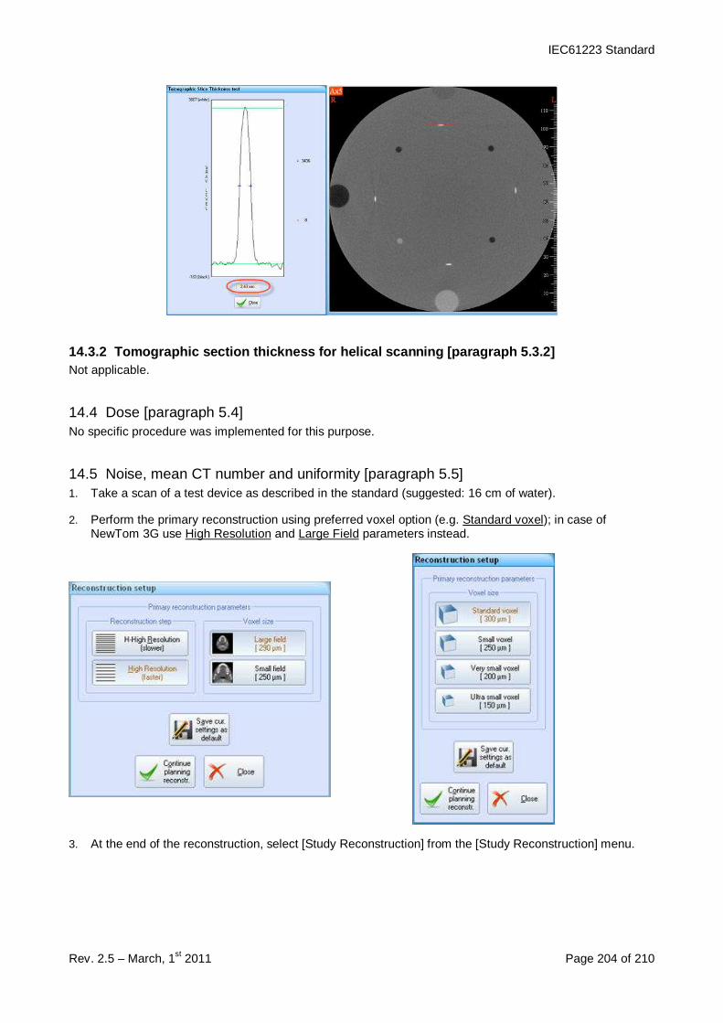
IEC61223 Standard
Rev. 2.5 – March, 1st 2011 Page 204 of 210
14.3.2 Tomographic section thickness for helical s canning [paragraph 5.3.2]Not applicable.
14.4 Dose [paragraph 5.4]No specific procedure was implemented for this purpose.
14.5 Noise, mean CT number and uniformity [paragraph 5.5]1. Take a scan of a test device as described in the standard (suggested: 16 cm of water).
2. Perform the primary reconstruction using preferred voxel option (e.g. Standard voxel); in case ofNewTom 3G use High Resolution and Large Field parameters instead.
3. At the end of the reconstruction, select [Study Reconstruction] from the [Study Reconstruction] menu.

IEC61223 Standard
Rev. 2.5 – March, 1st 2011 Page 205 of 210
4. Press the 100% button on the toolbar to enlarge the reconstruction area to the maximum.
5. Set the slice thickness to 0.5mm.
6. Move the Roi to reconstruct the volume where it has the maximum width, then press the right button ofthe mouse to run the Study reconstruction.
7. Open the study and visualize axial images. Set the single axial mode and browse the images till asection with the maximum diameter is showed.
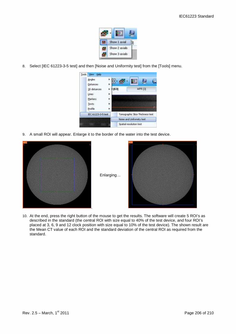
IEC61223 Standard
Rev. 2.5 – March, 1st 2011 Page 206 of 210
8. Select [IEC 61223-3-5 test] and then [Noise and Uniformity test] from the [Tools] menu.
9. A small ROI will appear. Enlarge it to the border of the water into the test device.
.
Enlarging…
10. At the end, press the right button of the mouse to get the results. The software will create 5 ROI’s asdescribed in the standard (the central ROI with size equal to 40% of the test device, and four ROI’splaced at 3, 6, 9 and 12 clock position with size equal to 10% of the test device). The shown result arethe Mean CT value of each ROI and the standard deviation of the central ROI as required from thestandard.
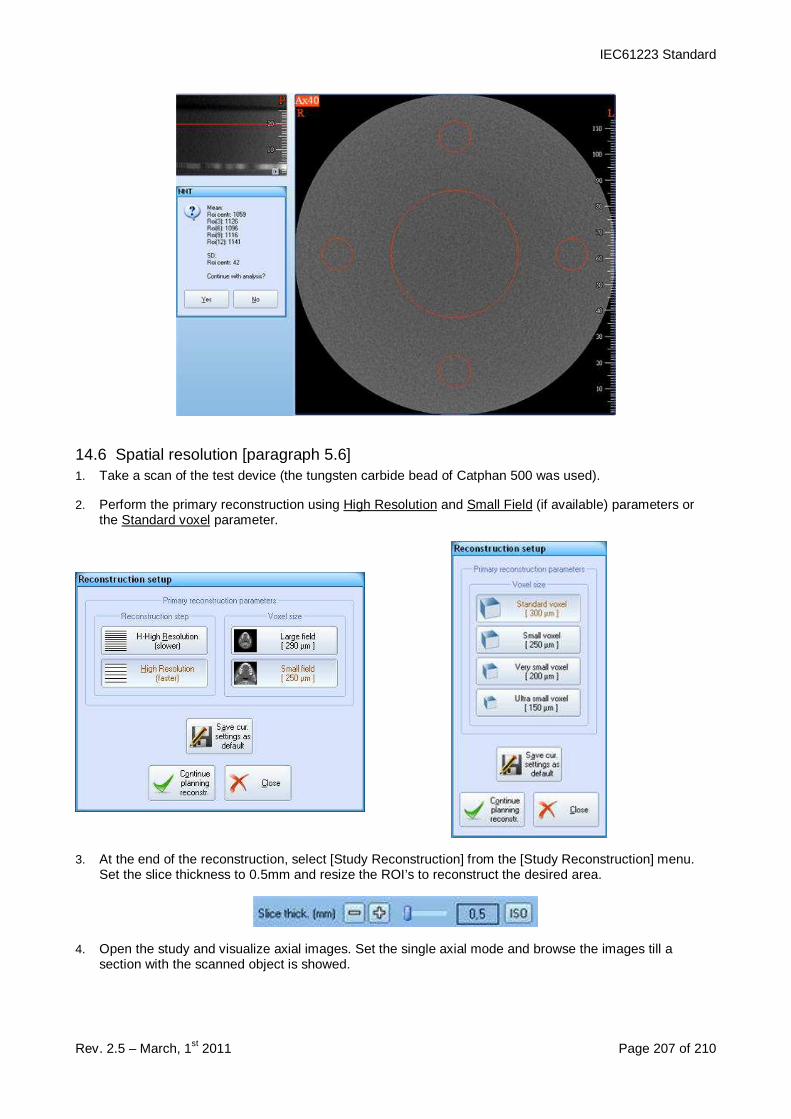
IEC61223 Standard
Rev. 2.5 – March, 1st 2011 Page 207 of 210
14.6 Spatial resolution [paragraph 5.6]1. Take a scan of the test device (the tungsten carbide bead of Catphan 500 was used).
2. Perform the primary reconstruction using High Resolution and Small Field (if available) parameters orthe Standard voxel parameter.
3. At the end of the reconstruction, select [Study Reconstruction] from the [Study Reconstruction] menu.Set the slice thickness to 0.5mm and resize the ROI’s to reconstruct the desired area.
4. Open the study and visualize axial images. Set the single axial mode and browse the images till asection with the scanned object is showed.
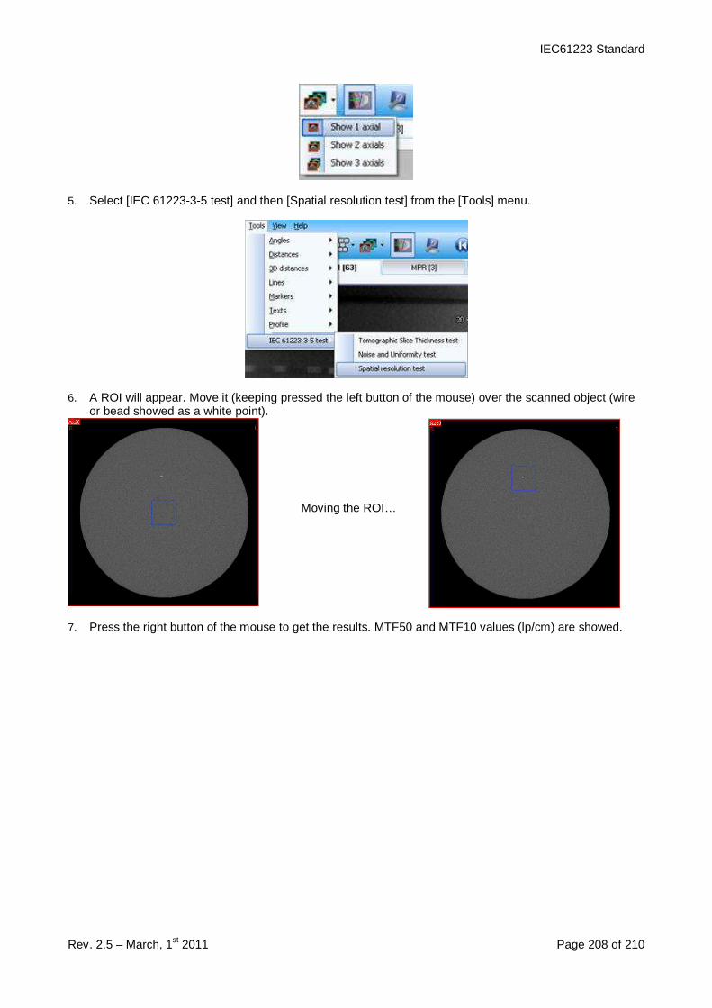
IEC61223 Standard
Rev. 2.5 – March, 1st 2011 Page 208 of 210
5. Select [IEC 61223-3-5 test] and then [Spatial resolution test] from the [Tools] menu.
6. A ROI will appear. Move it (keeping pressed the left button of the mouse) over the scanned object (wireor bead showed as a white point).
Moving the ROI…
7. Press the right button of the mouse to get the results. MTF50 and MTF10 values (lp/cm) are showed.
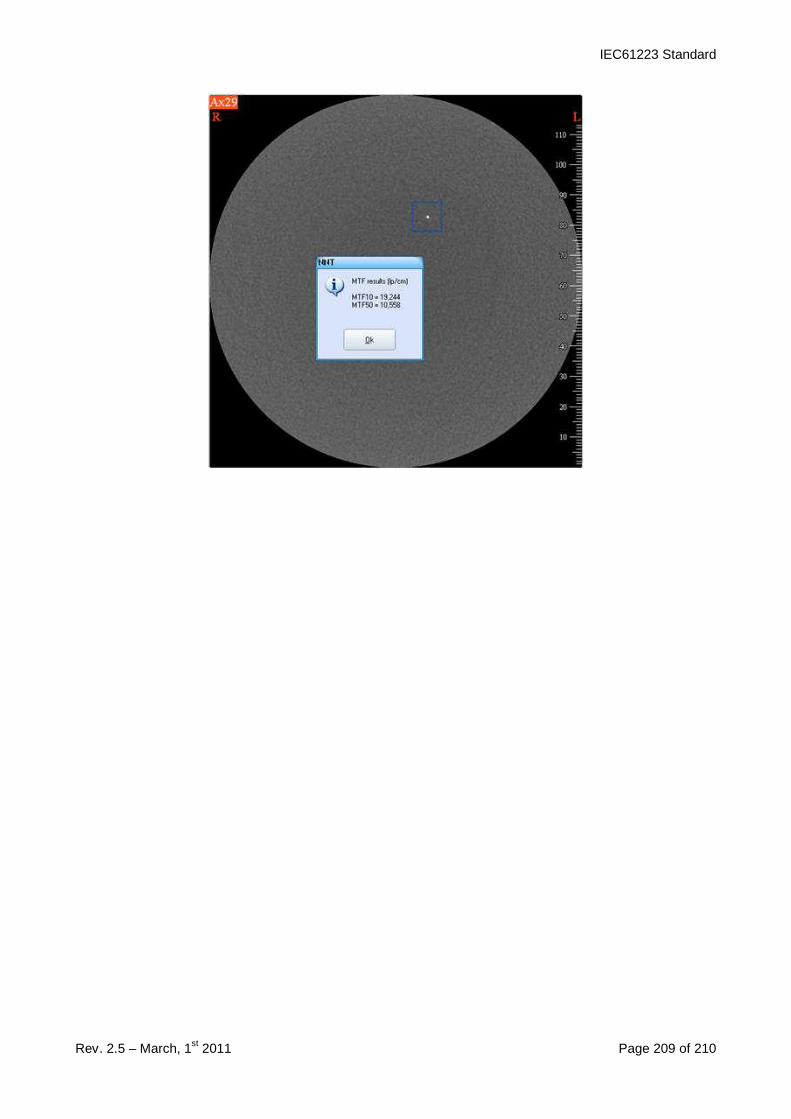
IEC61223 Standard
Rev. 2.5 – March, 1st 2011 Page 209 of 210
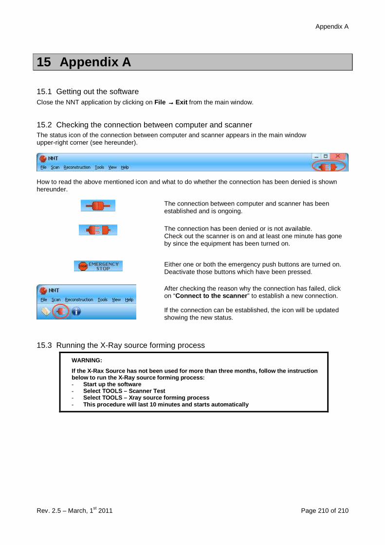
Appendix A
Rev. 2.5 – March, 1st 2011 Page 210 of 210
15 Appendix A
15.1 Getting out the softwareClose the NNT application by clicking on File →→→→ Exit from the main window.
15.2 Checking the connection between computer and scannerThe status icon of the connection between computer and scanner appears in the main windowupper-right corner (see hereunder).
How to read the above mentioned icon and what to do whether the connection has been denied is shownhereunder.
The connection between computer and scanner has beenestablished and is ongoing.
The connection has been denied or is not available.Check out the scanner is on and at least one minute has goneby since the equipment has been turned on.
Either one or both the emergency push buttons are turned on.Deactivate those buttons which have been pressed.
After checking the reason why the connection has failed, clickon “Connect to the scanner ” to establish a new connection.
If the connection can be established, the icon will be updatedshowing the new status.
15.3 Running the X-Ray source forming process
WARNING:
If the X-Rax Source has not been used for more than three months, follow the instructionbelow to run the X-Ray source forming process:- Start up the software- Select TOOLS – Scanner Test- Select TOOLS – Xray source forming process- This procedure will last 10 minutes and starts auto matically