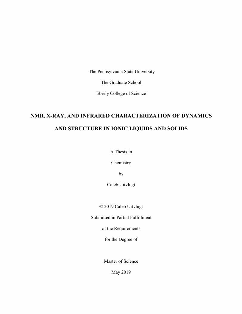
The Pennsylvania State University

The Graduate School

Eberly College of Science

NMR, X-RAY, AND INFRARED CHARACTERIZATION OF DYNAMICS

AND STRUCTURE IN IONIC LIQUIDS AND SOLIDS

A Thesis in

Chemistry

by

Caleb Uitvlugt

© 2019 Caleb Uitvlugt

Submitted in Partial Fulfillment

of the Requirements

for the Degree of

Master of Science

May 2019

ii

The thesis of Caleb Uitvlugt was reviewed and approved* by the following:

Mark Maroncelli

Distinguished Professor of Chemistry

Thesis Adviser

Scott A. Showalter

Associate Professor of Chemistry, Biochemistry, & Molecular Biology

Graduate Program Chair

Alexey Silakov

Assistant Professor of Chemistry

Michael Hickner

Professor of Materials Science & Engineering, Chemical Engineering

Philip Bevilacqua

Distinguished Professor of Chemistry, Biochemistry, & Molecular Biology

*Signatures are on file in the Graduate School.

iii

Abstract

In this work, the structure and dynamics of ionic liquid systems were investigated using

nuclear magnetic resonance (NMR) spectroscopy, differential scanning calorimetry (DSC), X-ray

scattering, and infrared (IR) spectroscopy. Two studies of the ionic liquid 1-butyl-3-

methylimidazolium tetrafluoroborate ([Im41][BF4]) were performed. These are described in

Chapter 1. One entailed studying the rotation of dimethylbenzene (DMBz) analogues and the other

rotation and translational diffusion in mixtures of [Im41][BF4] with the polar aprotic solvent

acetonitrile (ACN). A third study was conducted of the solid form of the ionic liquid

trimethyldecylammonium bis(perfluoroethylsulfonyl)imide ([N10,111][beti]) or DTAB.

The first set of rotational diffusion studies analyzed solutions of 1,4-dimethylbenzene-d10

(DMBz), 1,4-dimethylpyridinium-d7 hexafluorophosphate (DMPy), and p-tolunitrile-d7 (CMBz)

in [Im41][BF4]. These measurements, combined with molecular dynamics (MD) simulations

performed by Chris Rumble, investigated the effects of molecular size, shape, and electrostatics

on rotational dynamics in ionic liquids. For the second project, T1 relaxation times were measured

in a set of mixtures ranging from neat [Im41][BF4] to neat ACN with benzene as a solute. T1

relaxation measurements were taken of [Im41][BF4], ACN, and benzene to investigate the

rotational dynamics of a simple solutes as well as the solvent ions and the mixture was used to ask

if there are fundamental differences. The NMR measurements gave the average rotation times of

the [Im41][BF4] + ACN mixture, which were used by Brian Conway as a point of comparison for

MD simulations.

The third study examines the solid phase of the ionic compound [N10,111][beti] which forms

a unique optically clear solid near room temperature. Preliminary X-ray diffraction (XRD) and 13C

nuclear magnetic resonance (NMR) measurements indicated a superposition of order and

amorphous structure in the solid phase. Subsequent DSC, X-ray scattering, 2H NMR, and infrared

iv

spectroscopy data are used to attempt to assign the solid phase of DTAB to three possible

frameworks: plastic crystal, glacial state, and Frank-Kasper phases.

v

Table of Contents List of Figures ............................................................................................................................... vii

List of Tables ................................................................................................................................. ix

Ionic Liquid Nomenclature ..............................................................................................................x

Chapter 1. Rotation in Ionic Liquids ...........................................................................................1

1.1. Introduction ...........................................................................................................................1

1.2. Solute Rotation in Ionic Liquids ...........................................................................................2

1.3. Solute Dynamics in an Ionic Liquid ......................................................................................4

A. Experimental ........................................................................................................................4

B. Results and Discussion ........................................................................................................5

1.4. Solute and Solvent Dynamics in an IL and Acetonitrile Mixture .........................................6

A. Introduction .........................................................................................................................6

B. Experimental ........................................................................................................................6

C. Results and Discussion ........................................................................................................7

Chapter 2. [N10,111][beti], a Distinctive Ionic Solid ...................................................................11

2.1. Introduction .........................................................................................................................11

A. Preliminary NMR Data ......................................................................................................11

B. Preliminary X-ray Data ......................................................................................................12

2.2. Types of Solids ....................................................................................................................14

A. Plastic Crystals ..................................................................................................................14

B. Glacial States .....................................................................................................................17

C. Frank-Kasper Phases..........................................................................................................18

2.3. Differential Scanning Calorimetry ......................................................................................20

A. Introduction .......................................................................................................................20

B. Experimental ......................................................................................................................21

vi

C. Results ................................................................................................................................21

2.4. X-ray Scattering ..................................................................................................................24

A. Introduction .......................................................................................................................24

B. Results ................................................................................................................................24

C. Time Evolution of DTAB ..................................................................................................27

2.5. 2H NMR ...............................................................................................................................30

A. Introduction .......................................................................................................................30

B. Results ................................................................................................................................31

C. Discussion ..........................................................................................................................33

2.6. Infrared Spectroscopy .........................................................................................................35

A. Introduction .......................................................................................................................35

B. Results ................................................................................................................................36

2.7. Discussion of the Nature of the DTAB Solid ......................................................................38

A. Is the DTAB Solid a Plastic Crystal? ................................................................................38

B. Is the DTAB Solid a Glacial State? ...................................................................................39

C. Is the DTAB Solid Forming Frank-Kasper Phases? ..........................................................40

2.8. Conclusion ...........................................................................................................................42

Chapter 3. Summary and Conclusions .....................................................................................43

Appendix: NMR Calibration ......................................................................................................45

References ..................................................................................................................................52

vii

List of Figures Figure 1.1. 2H NMR probe molecules ............................................................................................4

Figure 1.2. Rotation times as a function of temperature for probe molecules .................................5

Figure 1.3. Deuterated [Im41][BF4] ..................................................................................................6

Figure 1.4. T1 times as a function of viscosity in [Im41][BF4]/ACN mixtures ...............................7

Figure 1.5. Simple pulsed field gradient NMR pulse sequence .......................................................9

Figure 1.6. Comparison of Simulated and Experimental Diffusion Coefficients ..........................10

Figure 2.1. [N10,111][Tf2N] and [N10,111][beti] structures ................................................................11

Figure 2.2. 13C spectra of [N10,111][beti] at 20 °C and 50 °C .........................................................11

Figure 2.3. X-ray diffraction spectra of [N10,111][Tf2N] and [N10,111][beti] ...................................12

Figure 2.4. NMR linewidths for 1H and 19F of [P1224][PF6] ..........................................................16

Figure 2.5. Low-frequency Raman spectra of triphenyl phosphite ...............................................17

Figure 2.6. Differential scanning calorimetry heating curve of [Nip311][Tf2N]..............................20

Figure 2.7. Differential scanning calorimetry curves of [N10,111][Tf2N], [N10,111][beti], and

[Pr10,1][beti] ....................................................................................................................................22

Figure 2.8. Crystal structure of [N12,111][Br] ..................................................................................26

Figure 2.9. Wide-angle X-ray scattering of [N10,111][Br], [N10,111][Tf2N], [N10,111][beti], and

[Pr10,1][beti] ....................................................................................................................................26

Figure 2.10. Isothermal aging of [N10,111][beti] X-ray scattering data at 17 °C ............................28

Figure 2.11. Carbon-deuterium bond against a magnetic field and a Pake doublet ......................30

Figure 2.12. 2H NMR lineshape data of DTAB-d21 .......................................................................32

Figure 2.13. Isothermal aging of DTAB-d21 2H NMR lineshape data at 17 °C and 10 °C ............32

Figure 2.14. Comparison of DTAB-d21 lineshape against nonadecane-d40 and deuterated

polyethylene ...................................................................................................................................33

Figure 2.15. Cisoid and transoid conformations of [beti]- .............................................................35

viii

Figure 2.16. Temperature dependent infrared spectra of [N10,111][beti] ........................................36

Figure 2.17. Arrhenius plot of relative infrared peak heights for [N10,111][beti] ............................37

Figure A.1. Temperature calibration for 300 MHz and 500 MHz NMR instruments using

methanol and ethylene glycol ........................................................................................................46

Figure A.2. Comparison of diffusion coefficients between pulsed field gradient NMR and

molecular dynamics simulations ....................................................................................................47

Figure A.2. Comparison of experimental pulsed field gradient diffusion coefficients against

literature and simulation values .....................................................................................................48

Figure A.3. Solid-echo NMR pulse sequence ................................................................................49

ix

List of Tables Table 2.1. Calorimetric Data for [N10,111][beti], [Pr10,1][beti], and [N10,111][Tf2N] ........................22

Table 2.2. X-ray scattering q ranges ..............................................................................................25

Table 2.3. Summary of solid phases ..............................................................................................42

x

Ionic Liquid Nomenclature

Nomenclature used to denote ionic liquid components in this thesis: Ionic liquids are designated according to cation type Im, Py, P, and N together with numbers indicating the length of appended n-alkyl chains, i, j, k, l. Ionic liquids are labeled [cation][anion]. For example, [Im41][BF4] is 1-butyl-3-methylimidazolium tetrafluoroborate.

NNRnRm

NRm

NRm Rn

RiN

Rj RkRl

F3C SO

ON S CF3

O

OC2F5 S

O

ON S C2F5

O

O

"Immn+" "Prmn

+"

imidazolium pyridinium

"Nijkl+""Pym

+"

ammoniumpyrrolidinium

"Tf2N-" "beti"

FB

F FF

FP F

F

FFF

Cations

Anions

BF4-

PF6-

1

Chapter 1: Rotation in Ionic Liquids

1.1 Introduction

Ionic liquids (ILs), defined as salts with melting temperatures at or below 100 °C, have

many favorable properties such as low vapor pressure, high thermal stability, and are generally

chemically inert1. ILs have a lot of potential for various applications because their viscosity,

density, and other physical properties are tunable through selection of the cation and anion pair or

through modification of the functional groups appended to these ions. For example, ILs tuned for

low viscosity could be used as green solvents for reactions2 and battery electrolytes3. To properly

utilize ILs, and guide the best choice of cation and anion, a fundamental understanding of their

properties is necessary. As a means of probing the friction operating on solutes undergoing

reactions, we have studied rotational dynamics in the prototypical ionic liquid 1-butyl-3-

methylimidazolium tetrafluoroborate ([Im41][BF4]) and its mixtures with a polar protic solvent.

2

1.2 Solute Rotation in Ionic Liquids

I contributed to two projects that focused on the rotational diffusion of solutes in the ionic

liquid [Im41][BF4]. A combination of molecular dynamics (MD) simulations and NMR T1

relaxation experiments were conducted to elucidate the molecular origins of friction on rotational

motion in ionic liquids. These two studies are now published as Refs 4 and 5.

In the MD simulations, rotations of molecules can be directly observed in model systems.

In such a model the cations, anions, and solute molecules are objects with defined properties such

as size, shape, and partial charge. These molecules are initially equilibrated, and then classical

trajectory data is collected over hundreds of nanoseconds. To characterize rotations from these

trajectories in an average manner appropriate for comparison to experiment, rotational time

correlation functions (RTCFs), are calculated.

𝐶𝐶𝑟𝑟𝑟𝑟𝑟𝑟(2) = 3

2⟨𝑢𝑢�(0) ∙ 𝑢𝑢�(𝑡𝑡)⟩2 − 1

2 (1)

In this expression 𝑢𝑢� is the direction of some particular bond within a molecule and the brackets

indicate averaging over like molecules and time. The RTCF characterizes the timescales of

different motions involved in rotation6. It decays from 1 at t = 0 down to 0 at long times. By fitting

this decay, time constants for the rotational motion can be extracted.

NMR can experimentally access the rotations of molecules through observation of nuclear

spin relaxation. For an NMR active nucleus, the rotation of the molecule is weakly coupled to the

relaxation of the nuclear spins. There are multiple mechanisms for the relaxation of nuclear spins

such as dipole-dipole interactions, chemical shift anisotropy, and quadrupolar interactions. Here I

will discuss the case of deuterium spin relaxation, in which case, the quadrupolar interactions

dominate the relaxation of a deuterium spin characterized by a spin-lattice relaxation time T17.

𝑇𝑇1−1 = 3𝜋𝜋2

10�1 + 1

3𝜂𝜂𝑄𝑄2� 𝜒𝜒2�𝑗𝑗(𝜔𝜔0) + 4𝑗𝑗(2𝜔𝜔0)� (2)

3

Values of ηQ and χ2, the asymmetry parameter and the quadrupole coupling constant respectively,

were calculated for each species studied using electronic structure calculations4. T1 relates to

rotation occurring at the Larmor frequency, (ω0) and its overtone (2ω0) because j(ω) in Eq 2 is the

spectral density of rotational motion.

𝑗𝑗(𝜔𝜔) = ∫ 𝐶𝐶𝑟𝑟𝑟𝑟𝑟𝑟(2)∞

0 (𝑡𝑡) cos(𝜔𝜔𝑡𝑡)𝑑𝑑𝑡𝑡 (3)

Seen in Equation 3, the spectral density function is the Fourier transform of the RTCF, the function

output by the MD simulations. By measuring the T1 relaxation time, we have a point of comparison

to validate the MD simulations. There is an additional result seen in Equation 3. The spectral

density function is frequency dependent. The cos(ωt) term can be reduced to a constant if the value

ωt does not change for the range of the RTCF. In this case the spectral density terms reduce to the

integral rotation time (τrot), i.e. 𝜏𝜏𝑟𝑟𝑟𝑟𝑟𝑟 = 𝑗𝑗(0) = ∫ 𝐶𝐶𝑟𝑟𝑟𝑟𝑟𝑟(2)∞

0 (𝑡𝑡)𝑑𝑑𝑡𝑡. This simplification provides

𝑇𝑇1−1 = 3𝜋𝜋2

10�1 + 1

3𝜂𝜂𝑄𝑄2� 𝜒𝜒2𝜏𝜏𝑟𝑟𝑟𝑟𝑟𝑟 when 𝜏𝜏𝑟𝑟𝑟𝑟𝑟𝑟𝜔𝜔0 ≪ 1. (4)

in which there is an inverse relationship between the T1 time and τrot. The region where the

condition 𝜏𝜏𝑟𝑟𝑟𝑟𝑟𝑟𝜔𝜔0 ≪ 1 holds is termed the extreme narrowing limit. This region provides for easy

comparison between the MD simulation and experiment, but the frequency dependent behavior is

lost, yielding only an averaged rotation time. The two rotational diffusion projects I worked on

used 2H T1 measurements within the extreme narrowing limit to simplify interpretation of the

NMR data.

4

1.3 Solute Dynamics in an Ionic Liquid

A. Experimental:

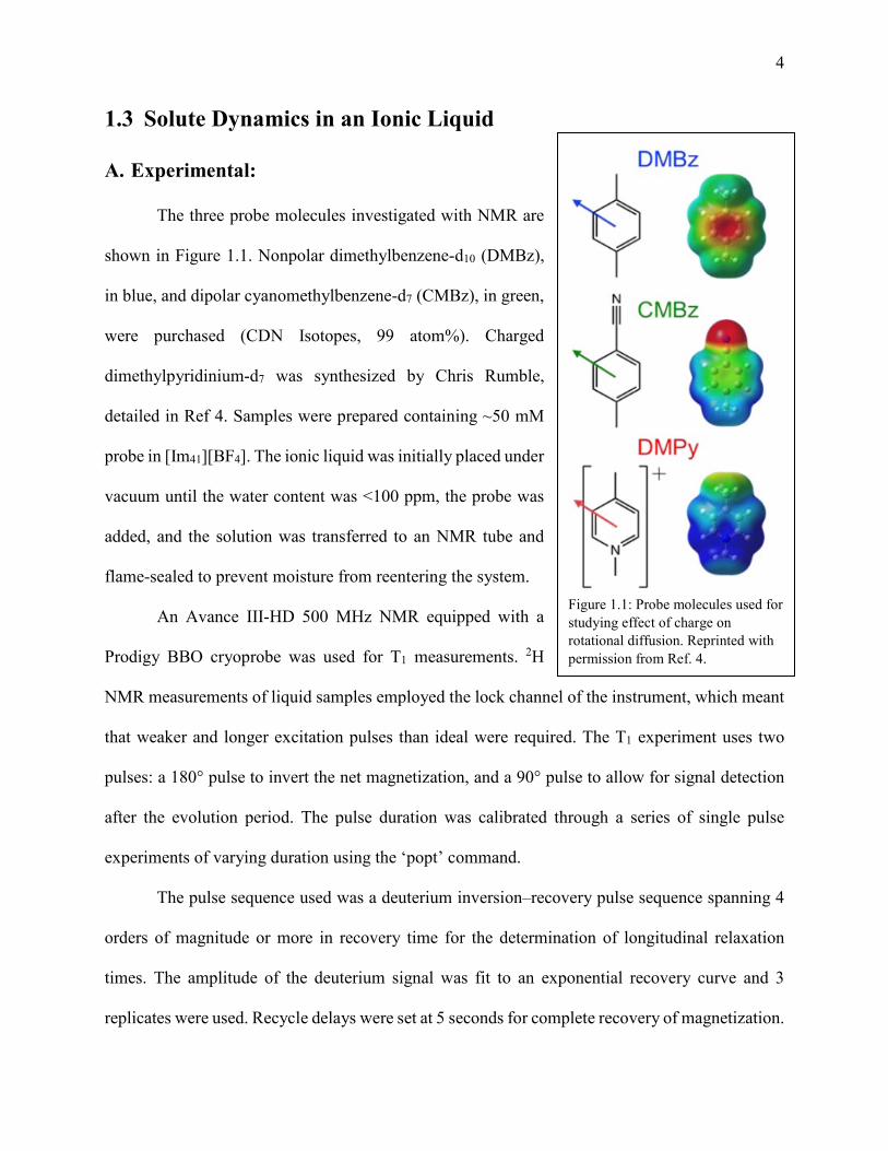
The three probe molecules investigated with NMR are

shown in Figure 1.1. Nonpolar dimethylbenzene-d10 (DMBz),

in blue, and dipolar cyanomethylbenzene-d7 (CMBz), in green,

were purchased (CDN Isotopes, 99 atom%). Charged

dimethylpyridinium-d7 was synthesized by Chris Rumble,

detailed in Ref 4. Samples were prepared containing ~50 mM

probe in [Im41][BF4]. The ionic liquid was initially placed under

vacuum until the water content was <100 ppm, the probe was

added, and the solution was transferred to an NMR tube and

flame-sealed to prevent moisture from reentering the system.

An Avance III-HD 500 MHz NMR equipped with a

Prodigy BBO cryoprobe was used for T1 measurements. 2H

NMR measurements of liquid samples employed the lock channel of the instrument, which meant

that weaker and longer excitation pulses than ideal were required. The T1 experiment uses two

pulses: a 180° pulse to invert the net magnetization, and a 90° pulse to allow for signal detection

after the evolution period. The pulse duration was calibrated through a series of single pulse

experiments of varying duration using the ‘popt’ command.

The pulse sequence used was a deuterium inversion–recovery pulse sequence spanning 4

orders of magnitude or more in recovery time for the determination of longitudinal relaxation

times. The amplitude of the deuterium signal was fit to an exponential recovery curve and 3

replicates were used. Recycle delays were set at 5 seconds for complete recovery of magnetization.

Figure 1.1: Probe molecules used for studying effect of charge on rotational diffusion. Reprinted with permission from Ref. 4.

5

The temperature calibration is covered in Sec. A.1. The arrow on each molecule in Figure 1.1 gives

the vector accessed through the NMR experiment, i.e. the aromatic deuterons for each probe.

B. Results and Discussion:

Figure 1.2 shows the

rotation times as temperature

was varied from 297–338 K.

DMBz has the fastest

rotation, followed by DMPy,

and finally CMBz.

Intuitively, one might expect

the order from fastest to

slowest to be DMBz, CMBz,

then DMPy, i.e. ordering

solutes from nonpolar,

dipolar, to charged. Instead we observe ordering of nonpolar, charged, to dipolar. This reflects the

subtle differences in the interactions of localized solute charges with the solvent ions. DMPy has

the greatest total interaction with the solvent because it has a net charge. The local environment of

DMPy is a shell consisting predominantly of anions. CMBz however has a dipole that is localized

to the cyano-group. The local environment consists of both positively and negatively charged areas

oriented around the molecule. Rotation of the molecules requires a larger local environmental

response in CMBz than DMPy, leading to a slower rotation time for CMBz than DMPy.

Figure 1.2: Rotation times calculated from the T1 relaxation measurements versus temperature.

6

1.4 Solute and Solvent Dynamics in an IL and Acetonitrile Mixture

A. Introduction:

The second system I studied was the mixture of [Im41][BF4] with acetonitrile (ACN). The

high viscosities of many ILs limit their utility as solvents for synthesis and as electrolytes in

batteries, because it limits the rate of reactant and charge transport. One option to overcome this

limitation is to mix the IL with a less viscous conventional solvent, enhancing the fluidity of the

ionic liquid, but often still retaining many of the IL’s desirable properties. The binary mixture

[Im41][BF4] + ACN is completely miscible at room temperature8, making it a useful prototype of

an ionic + dipolar aprotic liquid mixture with which to investigate how rotational and translational

motion change with changing composition and viscosity. Brian Conway performed MD

simulations of the solvent mixtures from neat ACN to neat [Im41][BF4] with and without benzene

as a solute. I performed complimentary NMR T1 measurements; this work is detailed in Ref 5.

B. Experimental:

Deuterated ACN

was purchased in small

ampules from Cambridge

Isotope Laboratories and

opened just before sample

preparation to minimize

water contamination. [Im41][BF4] was deuterated at the single site shown in Figure 1.3 following

a procedure of a previous group member, Anne Kaintz8. The C(2) proton of the imidazolium ring

is the most acidic proton and was found to exchange when [Im41][BF4] is refluxed in 9:1 D2O: H2O

for eight hours. Deuteration was check via 1H NMR by measuring the relative depletion of peak

Figure 1.3: [Im41][BF4] with the most acidic hydrogen deuterated.

7

intensity before and after deuteration. This process achieved ~20% deuteration of the C2 carbon

and no detectable deuteration at the other carbon positions. The ionic liquid was then heated to

~50 °C and dried under vacuum until the water content was <100 ppm as measured by Karl Fisher.

The deuterated ACN was purchased in ampules from Cambridge Isotope Laboratories and opened

just before sample preparation to minimize water content. The components were weighed

separately and combined into NMR tubes, which were then flame-sealed to prevent evaporation

of ACN and uptake of water by the ionic liquid.

Because the relaxation times of acetonitrile, benzene, and the imidazolium cation were

typically very different, separate sets of delay times were used in this experiment to capture the

behavior of each component.

C. Results and Discussion:

The comparison between

experimental T1 times (triangles) and

simulated values (circles) is shown in

Figure 1.4. Acetonitrile T1 times are in

blue, the [Im41]+ cation times in red,

and the benzene solute times in

purple. The ordering of the three

molecules follows size, as ACN is the

smallest, followed by benzene, and

the largest and slowest is the [Im41]+

cation. Benzene was chosen as a

solute because it provided a natural extension of previous work by Chris Rumble and Anne Kaintz

Figure 1.4: T1 times for ACN (blue), Benzene (purple), and [Im41]+ (red). Comparison between experimental data (triangles) and MD simulations (circles). Reprinted with permission from Ref. 5.

8

using MD simulations and NMR T1 relaxation measurements in [Im41][BF4]6. It is interesting that

there is an approximate power law relationship between the T1 times and the viscosity of the

solution. One could expect for a mixture between two dissimilar solvents that as the composition

changes, the solvents do not mix completely; instead the solvents would form into regions with a

higher concentration of one solvent as is observed in mixtures of ionic liquids with water9. These

T1 data do not appear to indicate anything but nearly ideal mixing. T1 times measured using NMR

for the two solvents as well as the solute of benzene agree reasonably with the simulated times

over the span of the sampled viscosities, which provides confidence in the choice of parameters

used to model the mixture.

Closely related to rotation times are translational diffusion rates. Using the simulation

trajectories, translational diffusion coefficients for the two solvents and benzene were also

calculated and compared with pulsed field gradient (PFG) NMR measurements. Calculation of the

diffusion coefficients (D) from the MD simulations followed Equation 5.

𝐷𝐷 = 16

lim𝑟𝑟→∞

𝑑𝑑𝑑𝑑𝑟𝑟⟨�𝑟𝑟(𝑡𝑡) − 𝑟𝑟(0)�

2⟩ (5)

It is straightforward to follow the positions of molecules as a function of time, 𝑟𝑟(t), from which

the squared displacement of each molecule can be tracked. Averaging this quantity over all

molecules of a given type provides mean squared displacement ⟨�𝑟𝑟(𝑡𝑡) − 𝑟𝑟(0)�2⟩. At short times,

the mean squared displacement does not track diffusion because translational motion is dominated

by small scale vibrational and librational motions of the molecules moving and impacting against

adjacent molecules. Only at long times does the slope of the mean squared displacement over time,

reflect the diffusion coefficient of the molecules.

9

The PFG NMR

technique, shown in

Figure 1.58, uses a

different approach than

T1 relaxation to measure

the translational

diffusion coefficient. At

the start of the PFG

experiment, the net

magnetization is aligned

with the external magnetic field, or along the vertical z-axis in Figure 1.5. A radio frequency (r.f.)

pulse is applied that rotates the net magnetization 90°, into the xy-plane. This is followed by a

gradient pulse to induce a gradient of the magnetic field with respect to the z-axis, essentially

encoding the position of each spin along the z-axis. As the local magnetic field increases, it causes

the transverse magnetization to precess at higher frequencies, as seen at the top of Figure 1.5

following the first “g” pulse. After a wait time (Δ), a second matching gradient pulse reverse the

effects of the first gradient. If no diffusion occurred along the z-axis, this second pulse would

completely reverse the effects of the first gradient pulse, causing no signal attenuation. If there is

diffusion, the resulting NMR signal is attenuated in proportion to the distance moved. The

relationship between the initial signal area (I(0)) and the detected attenuated signal area (I(g)) is

provided by Equation 6.

𝐼𝐼(𝑔𝑔) = 𝐼𝐼(0)𝑒𝑒𝑒𝑒𝑒𝑒 �𝐷𝐷(𝛾𝛾𝛾𝛾𝑔𝑔)2 �∆ − 𝛿𝛿3− 𝜏𝜏

3�� (6)

Figure 1.5: PFG NMR experiment with a z-gradient magnetic field. Grey boxes are gradient pulses and white boxes are radio frequency pulses. Reprinted with permission from Ref. 8.

τ τ

10

D is the diffusion coefficient, the value we use to compare between experiment and simulation.

During the PFG experiment, there are two gradient pulses with a wait time between them (Δ). The

gradient pulse duration (δ), and the gradient pulse intensity (g) can be varied to determine the

diffusion coefficient. The gyromagnetic ratio (γ) is dependent on the nucleus selected. Gradient

pulses cause electrical eddy currents that add artifacts and noise to the spectrum, τ is the wait time

to allow these eddy currents to relax before any subsequent pulse is applied. For our experiments,

Δ and δ were held constant as g was varied to characterize the attenuation due to diffusion.

The comparison between MD simulated diffusion coefficients (red) and experimentally

measured values (blue) is shown in Figure 1.6. The separation between the data is not a constant

factor as there is a larger separation between experiment and simulation for the low viscosity data

than the high viscosity data. The simulation data agrees with previously published diffusion

coefficients published by Liang et al.10 It has been determined the NMR diffusion coefficients

were incorrectly measured as the gradient strength (g) was incorrectly reported during these

measurements. Section A.2 details the steps taken to calibrate the PFG NMR experiment. Future

PFG NMR

measurements

should utilize an

external standard

for scaling of the

diffusion

coefficients to a

literature value. Figure 1.6: Comparison of experimental (blue) and simulation (red) diffusion coefficients of benzene in the [Im41][BF4]/ACN mixture samples.

1.00E-02

1.00E-01

1.00E+00

1.00E+01

1.0E-01 1.0E+00 1.0E+01 1.0E+02 1.0E+03

Diffu

sion

Coe

ffici

ent (

m^2

/s)/

10^-

11

Viscosity (cP)

11

Chapter 2 [N10,111][beti] a Distinctive Ionic Solid

2.1 Introduction

The structure of DTAB is seen in Figure 2.1. DTAB is an ionic liquid with a melting

temperature of 31 °C, making it an optically clear solid at room temperature. No other ionic liquid

known forms an optically clear room-temperature solid of this sort; ionic liquids tend to form

glasses at much lower temperatures or polycrystalline solids near room temperature. When the

DTAB anion is substituted for [N(SO2CF3)2]-, ([Tf2N]) also shown in Figure 2.1, the ionic liquid

persists in the liquid phase to a much lower temperature, forming

a crystalline solid near -30 °C11. The unique nature of the solid

phase of DTAB spurred initial nuclear magnetic resonance

(NMR) and X-ray diffraction (XRD) experiments that were used

when deciding on a framework for further analyses of DTAB.

A. Preliminary NMR Data:

Figure 2.2 shows preliminary 13C NMR spectra of DTAB collected by a former student

Bernie O’Hare in

2009. The top

spectrum is at 20 °C,

in the solid phase,

and the spectrum on

the bottom is at 50

°C, in the liquid. The

50 °C spectrum, with

its sharp well-separated resonances, is typical of a spectrum of a liquid of small molecules. The

Figure 2.1: Structures of DTAB and [N10,111][Tf2N].

N

SN

SO

O

O

OC2F5 C2F5

beti

SN

SO

O

O

OF3C CF3

Tf2N(Liquid) (Solid)

[N10,111]+

Figure 2.2: 13C spectra of [N10,111][beti] at 20 °C (solid) and 50 °C (liquid).

12

spectrum of the solid shows much broader peaks, but many of the peaks are still resolved. Solid-

state systems typically produce much broader and less resolved spectra because molecular level

motions are no longer fast on the NMR timescale12. The fact that the 13C spectrum of DTAB in the

solid-state shows some resolution indicates the presence of motional narrowing greater than is

typical in a glassy or crystalline solid. Such motional narrowing is the result of molecular motions

within the solid phase of DTAB that I’ve attempted to characterize using NMR, as described in

Sec 2.5.

B. Preliminary X-ray Data:

Several years ago, Edward Castner Jr. our collaborator at Rutgers University, took the X-

ray diffraction (XRD) data shown in Figure 2.3. DTAB is plotted in red and [N10,111][Tf2N] in

black. These XRD spectra were taken at room temperature where DTAB is a solid and

[N10,111][Tf2N] a liquid. The spectra show the scattered intensity as a function of momentum

transfer, q, defined by q = (4π/λ)sinθ where λ is the x-ray wavelength and θ is the scattering angle.

Large q corresponds to intramolecular distances while small q are intermolecular distances.

Narrow peaks in the XRD spectrum indicate a highly

ordered structure like that expected for a crystal. Broad

peaks indicate amorphous structure characteristic of a

liquid or glass. Both DTAB and [N10,111][Tf2N] have broad

intramolecular peaks. For lower q, the intermolecular

scale, [N10,111][Tf2N] has additional broad peaks while the

peaks of DTAB are sharper and more distinct, indicating

some degree of crystallinity in the solid phase of DTAB. It is unusual that both crystalline and

amorphous structure are present in the solid phase.

Figure 2.3: XRD spectra of DTAB (red) and [N10,111][Tf2N] (black) both spectra taken at 25 °C. Unpublished results.

Room Temp XRD

13

The preliminary NMR and X-ray data suggest that the solid phase formed by DTAB is

unusual. The research in this chapter is aimed to explore that nature of the solid in more detail.

14

2.2 Types of Solids

Solid phases of molecular compounds range from glassy to crystalline solids. A crystalline

solid is: “a crystal structure is a regular arrangement of atoms of molecules.13” Additionally, the

average position of an atom within the crystal structure does not change with time. A crystalline

solid is well ordered and it takes substantial energy is usually required to change a crystalline solid

to a liquid. On the other end is the glassy solid. Glassy solids are amorphous solids where the

arrangement of atoms or molecules is random and disordered, like a liquid. A glass to liquid state

transition requires less energy than a crystal to liquid transition because there is less ordering in

the solid phase.

The preliminary data from XRD indicates that DTAB is not simply an amorphous solid or

an ordered solid, but a superposition of both. The NMR data indicates that there is significant

motion occurring into the solid phase of DTAB. In this thesis, I will discuss three different types

of solids: plastic crystals, glacial solids, and Frank-Kasper phases as possible frameworks for

understanding the structure and dynamics of DTAB. The general features of these solids are

described below.

A. Plastic Crystals:

The classification “plastic crystal” stems from the fact that some organic crystals,

particularly those comprised of quasi-spherical molecules, have high plasticity14 rather than being

brittle, as is the case for “normal” organic crystals. Plastic crystals possess long-range translational

order but are orientationally disordered. Typically, a plastic crystalline phase is not the only solid

phase formed by a compound. Plastic crystals are often observed to undergo multiple solid-solid

phase transition; they form crystalline solids at lowest temperatures and different rotational

motions become less restricted as temperature is increased. The enhancement of orientational and

15

rotational motions as temperature is increased can be a sudden process, reflected in a phase change,

or a gradual process. In either case, the entropy changes from plastic crystal to liquid or between

two plastic crystalline phases are smaller in magnitude than the entropy change between a

crystalline solid and a liquid. For this reason, Timmerman proposed one metric for determining

whether a compound is a plastic crystal is that it possesses a low entropy of fusion (<20 J K-1 mol-

1)15.

The dynamics within a plastic crystal are often complex. Cyclohexane, as discussed in a

paper by McGrath et al. provides an entry point16. Cyclohexane forms a single plastic crystalline

phase between -87 °C and its melting point, 6 °C. McGrath and Weiss considered three

mechanisms for the dynamics within cyclohexane: rotational, translational, and conformational.

They measured 1H, 13C, and 2H lineshapes as a function of temperature. The different nuclei

experienced changes to their lineshapes at different temperatures within the plastic crystalline

phase of cyclohexane. Through an analysis of the different relaxation mechanisms involved for

the different nuclei, McGrath et al. determined time scales for the motions of cyclohexane, most

notably rotation of molecules occurring on μs-ns time scales.

More recent examples of plastic crystals include organic ionic plastic crystals (OIPCs).

OIPCs are ionic compounds made from imidazolium17, phosphonium18, and ammonium19 cations

usually combined with smaller inorganic anions that form plastic crystals in the solid state. Jin et

al. studied the OIPC [P1224][PF6]20. Differential scanning calorimetry (DSC) showed this

compound to undergo 4 solid-solid phase transitions between the well-ordered crystal and the

liquid. Jin et al. used NMR lineshape measurements to examine the rotational motion within the

solid phases. An advantage of studying the compound ([P1224][PF6]) was that hydrogen and

fluorine are only contained in the cation and anion respectively, which enabled Jin et al. to observe

16

their motions independently. They found that some of the phase changes produced abrupt

linewidth changes in either the hydrogen or fluorine peaks, as shown in Figure 2.4. This behavior

indicates motion of the cation or anion are primarily involved in each transition. Jin et al. observed

four solid phases of [P1,224][PF6] labeled I-IV where IV is the lowest temperature solid phase. In

the NMR spectra, there are two changes observed. At low temperatures, there is a broad peak that

gradually narrows as the temperature increases. Additionally, a narrow peak appears on top of the

broad peak, indicating a growing fraction of [P1,224][PF6] is in a less restricted environment. Phase

IV shows a gradual decrease in the 1H and 19F linewidth. Jin et al. connect this to rotation of the

methyl and ethyl groups of the cation and isotropic tumbling of the anion respectively. The

transition to phase III produces linewidth jumps for both nuclei. This is attributed to rotation of

the cation around an individual axis. Phase II produces a dramatic change in the fluorine linewidth

while the change to hydrogen is less dramatic. Jin et al. connect this to diffusive motion of the

anion while the cation rotation is gradually becoming less restricted. The final solid-solid phase

transition to phase I does not have significant change in the fluorine lineshape as it is already

diffusive motion. The broad peak of the hydrogen disappears as the cation also undergoes diffusive

motion. NMR lineshape was used by Jin et al. to obtain a detailed understanding of molecular

Figure 2.4: NMR linewidths as a function of temperature for 1H (a) and 19F in the plastic crystal [P1224][PF6] Reprinted with permission from Ref. 20.

17

motions in an ionic compound. Similar measurements will be useful to characterize the molecular

motions of DTAB.

B. Glacial States:

Glacial states consist of nanocrystallites

imbedded in an amorphous phase. These states

may be formed when crystallization occurs near

the glass transition, creating conditions in which

only nm-scale crystallites can be formed before

further growth of the crystallites is halted.

Glacial states have only been clearly identified

in a small number of systems. One of the most

studied examples is triphenyl phosphite (TPP).

Guinet et al. used low-frequency Raman spectra

to characterize the glacial state formed by TPP

forms under specific temperature protocols.

One method of forming the glacial state of TPP is to hold it isothermally at 220 K, ~20 K above

the glass transition temperature. Figure 2.5, from the paper by Guinet et al., demonstrates the

mixed nature of the glacial state21. The glacial state spectrum contains both broad and sharp peaks,

indicative of the amorphous and crystalline phases respectively. Additionally, the inset shows

development of the crystalline peaks over the course of an hour as the glacial state develops from

isothermal aging.

The only ionic compound so far reported to form a glacial phase is [N4111][Tf2N] by Faria

et al.22 [N4111][Tf2N] formed the glacial phase through two temperature protocols: rapid cooling

Figure 2.5: Low-frequency Raman of TPP as a supercooled liquid, a glacial state, and a crystal. The time dependence of the Raman spectrum is shown in the inset. Reprinted with permission from Ref. 21.

18

followed by slow heating, and isothermal aging. Faria et al. used Raman spectroscopy to

characterize the conformations of the Tf2N- anion, which can adopt into cisoid and transoid forms.

If the solid formed were a single crystal, only a single form of the anion is expected. The solid

phase formed by [N4111][Tf2N] through the isothermal aging method primarily adopted the cisoid

conformation, but the transoid conformation was present as well.

C. Frank-Kasper Phases:

Frank and Kasper originally observed FK phases in metal alloys23. Elemental metals

typically adopt body-centered cubic (BCC) or face-centered cubic (FCC) structures, which have 2

and 4 atoms per unit cell, respectively. In contrast, many metal alloys composed of 2 or more

elements adopt much more complex structures having anywhere from 12 up to 30 atoms per unit

cell. Driving the formation of these more complex FK structures is the desire to achieve topological

close packing (TCP) where the structures that have TCP have exclusively tetrahedral interstices13.

Packing in this manner can achieve a lower total energy than the other arrangements when the

main interactions involve central potentials.

In addition to alloys, FK phases have recently been found to occur in systems of simple

aqueous surfactants24 and neat diblock copolymers25. The surfactants and diblock copolymers form

into micelles that then organize into FK phases. In both the surfactant and the diblock copolymer

systems, FK phases were detected using small-angle X-ray scattering (SAXS) analysis. In the

SAXS spectra, numerous peaks are visible due to the large number of distinct sites in the unit cell.

In the case of the diblock copolymer, the FK phases were formed via isothermal aging like the

formation of the glacial state.

The three solid phases described above present comparisons for the analysis of DTAB.

Plastic crystals, glacial states, and FK phases all form in systems composed of molecules similar

19

to [N10,111][beti]. The spectroscopic techniques that are discussed in the remainder of this chapter

include differential scanning calorimetry (DSC), X-ray scattering, 2H NMR, and infrared (IR)

spectroscopy. DSC identifies the phase transitions and the temperatures of interest to help guide

subsequent experiments with the other techniques. The X-ray scattering data is used in both plastic

crystals and FK phases to examine the degree of ordering and identify the structure of the solid.

NMR lineshapes have been used in plastic crystals to examine the dynamics within the solid and

identify transitions in the motion. Infrared spectroscopy is used like Raman spectroscopy to

examine the possibility of a glacial state. Isothermal aging is a key component in the formation of

both the glacial state and the FK phases and is used in the NMR, X-ray, and IR analyses.

20

2.3 Differential Scanning Calorimetry

A. Introduction:

DSC measurements provide a starting point for the characterization of DTAB. DSC

compares the amount of heat required to change the temperature of a compound at a constant rate

against a reference with a known heat capacity. Here and in almost all cases the reference is simply

an empty pan. When the compound of interest undergoes a phase transformation, the amount of

heat required differs from the reference. An endothermic phase transition requires more heat

flowing to the sample to change the temperature at the same rate as the reference, whereas in an

exothermic phase transition heat flows out of the sample. Another type of transition is a glass

transition, signaled by an inflection point in the DSC curve, indicating an abrupt change in the heat

capacity of the sample. Data can either be collected upon heating or cooling the sample, but a

complete experiment includes both the heating and cooling curves.

Figure 2.6 shows a representative DSC curve of

the ionic compound [Nip311][Tf2N], taken from a

previous Maroncelli group paper26. The baseline heat

flow is negative, indicating that it is a heating curve.

There is an inflection point below 200 K, indicative of a

glass transition. The temperature of this transition (Tg) is

taken at the inflection point. At 225 K there is an

exothermic peak indicative of crystallization of the

sample. The two important pieces of information about

such a peak are the temperature of the transition (Tcr),

and the enthalpy of the transition. Tcr is determined from the onset of the transition. For this heating

Figure 2.6: DSC heating curve for [Nip311][Tf2N] from reference 16. Heating curve shows glass transition Tg, cold crystallization peak Tcr, and fusion peak Tfus. Reprinted with permission from Ref. 26.

21

curve, Tcr is measured from the left side of the peak at the point where the left slope intersects the

baseline. The enthalpy of the transition is the area under the curve multiplied by the calorimetric

constant, which is instrument dependent. The third peak near 280 K is an endothermic peak

indicative of fusion of the sample. The temperature of fusion (Tfus) and enthalpy of fusion are

determined in the same way as for the crystallization peak.

As illustrated in Figure 2.6, the temperature at which a sample crystallizes may be far

removed from the temperature at which it melts. This hysteresis is a kinetic effect in samples that

are readily supercooled. The extent of the hysteresis depends on the rate of heating and cooling. A

slower rate should reduce the size of the hysteresis. For a more complete understanding of the

behavior of a compound, multiple rates of temperature ramping should be used.

B. Experimental:

Data was collected on a TA Instruments Q2000 Modulated Differential Scanning

Calorimeter. The pans used to hold the samples and serve as a reference were “Tzero” aluminum

pans. Compounds studied were [N10,111][beti], [N10,111][Tf2N], and [Pr10,1][beti]. Samples were

melted prior to placing them in the sample pan. The heating/cooling protocol brought the sample

to 60 °C then cooled to -90 °C at 10 °C/min. The sample was then heated back to 60 °C at 10

°C/min. Table 2.1 contains the sample weights. Only single DSC scans of [N10,111][Tf2N] and

[Pr10,1][beti] collected to date. DTAB scans are similar to scans obtained by our collaborators Jim

Wishart and Bratoljub Milosavljevic.

C. Results:

DSC curves of DTAB and two other ionic liquids, [Pr10,1][beti] and [N10,111][Tf2N], used

for comparison are shown in Figure 2.7. Transition data are compiled in Table 2.1. DTAB ([N-

10,111][beti]) (red curve) has a relatively simple DSC scan. There is a single peak in the cooling run,

22

indicating a liquid to solid phase transition. The heating run shows a single peak for the solid-to-

liquid transition. There is a hysteresis of about 18 °C where DTAB is in a supercooled liquid state.

The ionic liquid [N10,111][Tf2N] (black curve) has a few more features in the DSC scan. In the

cooling curve there is no crystallization peak, just a change in heat flow near -45 °C which is not

consistent with crystallization at lower temperature upon heating. On the heating curve there are

two exothermic peaks indicative of cold crystallization. Upon further heating a melting peak is

observed.

Figure 2.7: DSC scans of [N10,111][beti] (red), [Pr10,1][beti] (blue), and [N10,111][Tf2N] (black).

- 10 °C/min

10 °C/min

Tc= 12 °CΔHc = -6.4 kJ/mol

Tcc = -57 °CΔHcc = -4.7 kJ/mol

Tcc = -45 °CΔHcc = -18.0 kJ/mol

Tm =16 °CΔHm = 38.7 kJ/mol

Tm = 30 °CΔHm = 7.9 kJ/mol

Table 2.1: Calorimetric Data Ionic liquid Tcr °C ΔcrH

kJ mol-1 Tfus °C ΔfusH

kJ mol-1 ΔfusS kJ mol-1 K-1

Sample weight (mg)

[N10,111][beti] 12 6.37 30 7.94 0.026 5.7

[Pr10,1][beti] – – – – – 6.8

[N10,111][Tf2N]1 -57, -45 4.69, 18.00 16 38.71 0.13 7.6

Tcr, ΔcrH, Tfus, and ΔfusH are the temperatures and enthalpies of crystallization and fusion. 1The crystallization temperatures for [N10,111][Tf2N] were measured upon heating whereas those of [N10,111][beti] were measured upon cooling.

23

[N10,111][Tf2N] provides a point of comparison with Mizuhata et al. as they examined a

series of [Nn,111][Tf2N] ionic liquids via DSC11. My values for the melting point and entropy of

fusion (ΔfusS) are 16 °C and 0.13 kJ mol-1 K-1 respectively, which are comparable with values

reported by Mizuhata et al. of 23 °C and 0.16 kJ mol-1 K-1. In examining where their DSC curve

intersects the baseline for [N10,111][Tf2N], their melting point is also ~16 °C. Comparison of the

cold crystallization peaks shows that on subsequent heating/cooling cycles, there is a single cold

crystallization peak. Multiple peaks are likely due to the sample not being uniform within the

aluminum pan and thus separate portions of the sample undergo the phase changes at slightly

different temperatures.

The third ionic liquid [Pr10,1][beti] does not have apparent melting or crystallization peaks.

Jin et al. report that there is a glass transition near -80 °C in [Pr10,1][Tf2N]26.

DTAB sits between the other two ionic liquids in terms of the phase changes. It has

crystallization and melting peaks unlike [Pr10,1][beti], but the entropy of these transitions are much

lower than those seen in [N10,111][Tf2N]. The ΔfusS is 0.026 kJ mol-1 K-1 for DTAB which is five

times less than for [N10,111][Tf2N] at 0.13 kJ mol-1 K-1. The difference in magnitude between the

two compounds indicates a difference in the degree of ordering in the solid phase. The larger the

entropy difference, the higher the degree of ordering in the solid phase. DTAB has a lower degree

of ordering than [N10,111][Tf2N] by a significant margin. The value of 0.026 kJ mol-1 K-1 is

comparable to Timmerman’s observation about plastic crystals (<0.02 kJ mol-1 K-1)15. The DTAB

DSC results are consistent with measurements taken by our collaborators Jim Wishart and

Bratoljub Milosavljevic. More measurements are being performed. Additional experiments

examining the scan rate are planned as one of the key identifiers of the glacial phase is a variation

in the solid formed based on scan rate22.

24

2.4 X-ray Scattering

A. Introduction:

Multiple techniques fall under the term X-ray scattering. All are used to characterize the

spatial structure of materials. A beam of monochromatic X-rays interacts with a sample. The X-

rays are scattered by the electrons in the sample and the measured interference pattern yields

information about the sample’s atomic structure. Sharp, well defined peaks indicate a more well-

ordered system, whereas broad and less intense peaks indicate a more disordered system.

Scattering at small angles/scatter vectors q reflect intermolecular distances and large q reflects

intramolecular distances. Lattice spacings d are related to q by d =2π/q.

To examine the possibility that the DTAB solid should be viewed as a type of FK phase, a

glacial state, or a plastic crystalline phase, markers in the X-ray scattering data are required. In the

case of FK phases a significant time dependence is often found for their formation. For example,

Lee et al. observed that block copolymer systems that form FK phases first order into a body-

centered cubic (BCC) structure during the first 5 hours of isothermal aging25. As aging continued,

the BCC peaks decay away and are slowly replaced by the final FK phase. It is unclear what

timescale to expect for similar changes in the DTAB system.

The formation of a glacial state should also be accompanied by a time evolution in the data.

Faria’s work on the glacial state of [N4,111][Tf2N] does not include X-ray scattering, but the Raman

data indicates formation of nanocrystallites during isothermal aging that should be visible by

XRD22. These nanocrystallites occur over a range of sizes and are enmbedded in an amorphous

phase, producing a complicated X-ray scattering pattern. The X-ray studies of the glacial state

formed by TPP show a q-4 dependence at q < 0.04 Å-1 (d>150 nm) due to the presence of a

distribution of nanocrystal sizes27.

25

Plastic crystals are typically more crystalline than a glacial state or FK phase. X-ray

scattering experiments reflect this, as the data can be fit to crystal structures19. One common aspect

of plastic crystals is that multiple solid-solid phase transitions are often visible as peaks in the

DSC. The different solid phases organize into different crystal structures17, which is reflected in

different sets of peaks at different temperatures in the X-ray scattering data.

X-ray scattering experiments were performed using a Xenocs Xeuss 2.0 instrument,

equipped with microfocus sealed tube (copper) with an X-ray wavelength of 1.54 Å (50 kV, 0.6

mA). Scattering data were collected under vacuum. Samples were prepared in 1 mm diameter

quartz capillaries and sealed with epoxy. Two instrumental setups were used to obtain different

scattering vector (q) ranges. For each setup the overall q range observable depended on the number

of images collected. These ranges are given in Table 2.2. Exposure times were 300 seconds except

the 60 °C and the initial 17 °C SAXS spectra of DTAB, which had an exposure time of 60 seconds

per image. The 2D images were converted into one-dimensional plots of scattering intensity I(q)

(arbitrary units) versus q by integrating semicircular portions of the images.

B. Results:

Four ionic compounds were examined in X-ray scattering experiments: [N10,111][beti]

(DTAB), [N10,111][Tf2N], [Pr10,1][beti], and [N10,111][Br]. The bromide was added as a reference

because it is a high-melting solid expected to have a well-ordered crystal structure similar to the

structure published for the homologous compound [N12,111][Br]28.

Table 2.2: X-ray Scattering Ranges Small angle X-ray scattering (SAXS) Wide angle X-ray scattering (WAXS)

Min. q (Å-1) Max. q (Å-1) Images Min. q (Å-1) Max. q (Å-1) Images 0.008 0.236 1 0.10 1.68 1 0.008 0.400 2 0.10 2.60 2 0.008 0.480 3 0.10 2.90 3

26

In the case of

crystalline [N12,111][Br],

shown in Figure 2.8, cations

organize into sheets of all

trans C12 chains. The cation

heads alternate with Br- anions

to form a polar region and the

alkyl tails remain mostly trans

but with a small twist and fill

a nonpolar domain between

the polar regions.

Figure 2.9 compares the X-ray scattering patterns of the four compounds. The [N10,111][Br]

data were recorded at 25 °C, because it has a melting point above 200 °C. The [N10,111][Tf2N] and

[Pr10,1][beti] data were taken at -60 °C, which is below Tcr of the [Tf2N] ionic liquid (-57 °C).

[Pr10,1][beti] is likely a

supercooled liquid at this

temperature. [N10,111][beti]

data were taken at 25 °C

after an isothermal aging

process, discussed in Sec.

C, and having been cooled

to low temperature. The

[N10,111][Br] spectrum, in Figure 2.9: WAXS spectra of [N10,111][Br] (green), [N10,111][Tf2N] (black), [N10,111][beti] (red), and [Pr10,1][beti] (blue).

0.1

1

10

100

1000

0.1 0.3 0.5 0.7 0.9 1.1 1.3 1.5 1.7

Inte

nsity

(arb

. Uni

ts)

q (1/Å)

Figure 2.8: Crystal structure of [N12,111][Br]. Reprinted with permission from Ref. 28.

27

green, shows peaks that are sharp and well defined. It is expected that the crystal structure of

[N10,111][Br] should be similar to that of the known structure of [N12,111][Br], with the main

difference being that the size of nonpolar domains would be slightly smaller. Initial attempts to fit

the unit cell parameters to the scattering pattern observed for [N10,111][Br] yielded several

possibilities similar to the [N12,111][Br] case.

There is a clear difference between the powder patterns shown by [N10,111][Br] (green),

[N10,111][Tf2N] (black), and the two beti compounds (red and blue). Both the [Tf2N] and [Br]

compounds have sharp, well defined peaks at regular intervals, indicating a high degree of order.

[N10,111][beti] (DTAB) in red has a much higher number of overlapping peaks, indicating there is

order, but the order is not regular throughout the sample. [Pr10,1][beti] in blue on the other hand

shows only 3 broad peaks common to most ionic liquids29. These broad peaks indicate [Pr10,1][beti]

is either a liquid or a glass and remains largely disordered at -60 °C.

These observations agree with the DSC results in that the much larger fusion entropy of

[N10,111][Tf2N] compared to DTAB suggests a much more ordered solid. While sharp peaks in the

DTAB spectrum indicate substantial order, the broad underlying scattering indicates substantial

amorphous character as well.

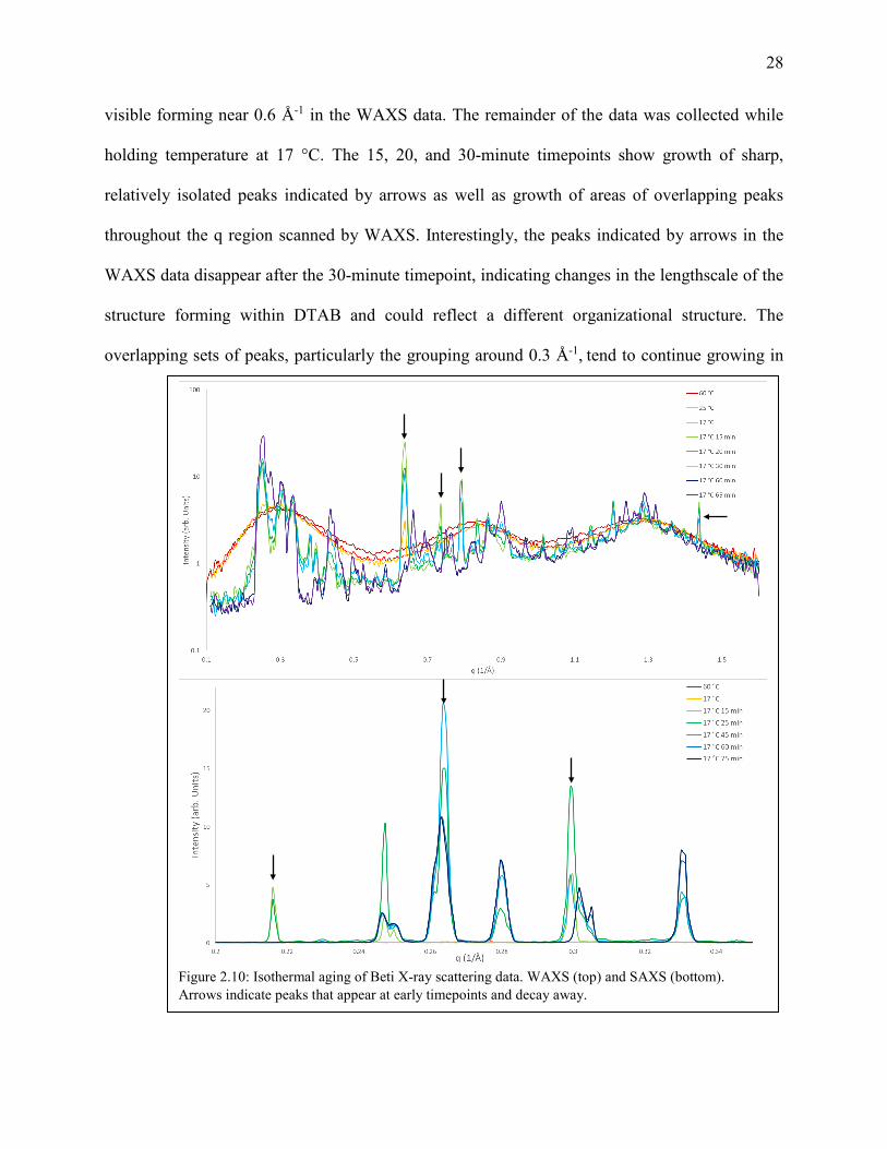
C. Time Evolution of DTAB

Figure 2.10 includes multiple temperatures and a time evolution of DTAB to elucidate the

formation of the solid. The top panel shows data recorded using the WAXS setup and the bottom

panel the SAXS setup. The 60 °C data (dark red) displays three broad peaks characteristic of ionic

liquids and similar to the [Pr10,1][beti] data in Figure 2.9 (blue). This was the starting point for the

set of experiments; DTAB in the liquid state. Similar broad peaks are visible in the 25 °C (red) and

initial 17 °C (orange) spectra. The initial 17 °C spectrum includes small sharper peaks, the most

28

visible forming near 0.6 Å-1 in the WAXS data. The remainder of the data was collected while

holding temperature at 17 °C. The 15, 20, and 30-minute timepoints show growth of sharp,

relatively isolated peaks indicated by arrows as well as growth of areas of overlapping peaks

throughout the q region scanned by WAXS. Interestingly, the peaks indicated by arrows in the

WAXS data disappear after the 30-minute timepoint, indicating changes in the lengthscale of the

structure forming within DTAB and could reflect a different organizational structure. The

overlapping sets of peaks, particularly the grouping around 0.3 Å-1, tend to continue growing in

Figure 2.10: Isothermal aging of Beti X-ray scattering data. WAXS (top) and SAXS (bottom). Arrows indicate peaks that appear at early timepoints and decay away.

29

intensity to the 60 and 65-minute timepoints. This is more expected for a liquid changing to a solid,

the peaks grow in intensity as a larger percentage of the compound adopts the final structure.

There are similar results in the SAXS data where peaks labeled with arrows grow in over

the first 30 minutes but disappear before the 60-minute mark. SAXS also provides a rough estimate

of the lattice spacings within DTAB as d =2π/q. The smallest q peaks are approximately at 0.21,

0.25, and 0.26 Å-1, which reflect distances of ~30, 25, and 24 Å respectively. 30 Å is a reasonable

size for a single micelle but is smaller than a supermolecular ordering of micelles as is expected in

FK phases. No small angle scattering was observed below the peak at 0.21 Å-1. Thus, the q-4

dependence expected in the formation of a distribution of crystallite sizes is not observed.

30

2.5 2H NMR

A. Introduction

In Chapter 1, I discussed the use of deuterium NMR T1 measurements to aid in

understanding rotational motion in ionic liquids4. Deuterium NMR is also a useful tool in

understanding motion in solid systems30, but there is much less freedom of motion in solids.

Interactions that are typically averaged in a liquid, such as electric quadrupolar and magnetic

dipolar interactions, now depend on molecular orientation within the solid12. This causes a

substantial broadening of the spectrum.

Deuterium has a nucleus of spin 1 and

so, in the presence of a magnetic field,

has three energy levels corresponding

to spin quantum numbers mz = +1, 0,

and -1 and two single-quantum

transitions among these levels.

The shape of the 2H spectrum indicates the nature of the solid phase. A crystalline solid

comprised of immobile molecules all oriented in a similar manner has two Lorentzian peaks from

the two allowed transitions. A powder sample also has two peaks, but each peak is broadly

distributed as seen in Figure 2.1131. This pattern is due to the various alignments different crystals

adopt relative to the instrument’s magnetic field. This line shape is called a Pake pattern, and is

typical of powder samples32. The splitting of the peaks in the Pake pattern is significant. In the

absence of molecular motion, The splitting between the outermost shoulders in a Pake doublet is

3CQ/2 and the splitting between the prominent inner peaks is 3CQ/4, where CQ is the quadrupolar

coupling constant7.

Figure 2.11: Illustration of the orientation of the carbon-deuterium bond against the magnetic field (left) and the Pake doublet (right). Reprinted with permission from Ref. 31.

31

Solid-state NMR measurements were taken on an Avance-III-HD solid state 500 MHz

instrument with a quadruple-tuned 4-mm cross polarized magic angle spinning (CPMAS) probe.

Samples were paced in 4 mm rotor tubes with a Vespel cap and held immobile as the NMR spectra

were collected. Spectra were recorded using a spin-echo pulse sequence, which involves two R.F.

pulses to rotate the net magnetization. Two pulses are used due to the rapid decay of the net

magnetization in the solid state. The initial 90° pulse rotates the net magnetization into the

detectable window, followed by a 30 μs delay time before the second 90° pulse which refocuses

the net magnetization. The magnetization refocuses based on the delay time and acquisition can

collect the refocused echo, enhancing the signal in comparison to a single pulse probe experiment.

1024 scans were used for all spectra, and a sweep width of 156 kHz was used to observe the entire

width of the Pake pattern, resulting in a spectrum taking 200 seconds to collect. Details on the

calibration of experimental parameters are discussed in Sec. A.3. The sample used for 2H lineshape

measurements, [N10,111][beti]-d21 (DTAB-d21) contained a perdeuterated decyl tail. It was

synthesized by Gary Baker at the University of Missouri.

B. Results

Presented in Figure 2.12a are 2H solid state spectra of DTAB-d21 at 10, 17, and 40 °C.

Calorimetric data indicate that the liquid-to-solid transition of DTAB occurs between 10 and 17

°C upon cooling, so two of the spectra are of the liquid state and one of the solid state. The peak

in the solid spectrum (10 °C) is significantly broader, as seen in the normalized spectra of Figure

2.12b. Recent work on the ionic compound [P1224][PF6] provides some insight into the significance

of the broadening upon solidification. The findings of Jin et al. are discussed in detail in sec. 2.320.

Jin et al. demonstrated that large-scale changes in the linewidths of 1H or 19F peaks at the phase

changes of [P1224][PF6] reflect changes in the molecular motion of the cation or anion respectively.

32

In DTAB, a broadening of the deuterium

peak reflects the fact that cation motion,

specifically motion of the deuterated decyl

tail, is markedly slowed as a result of

solidification.

To elucidate the isothermal aging

observed in the XRD experiments,

analogous isothermal aging experiments

were performed on DTAB-d21. The X-ray

data showed structural equilibration was

required to form a solid at 17 °C. Shown in

Figure 2.13 are the normalized spectra of

DTAB-d21 during isothermal aging at 17 °C

(left) and 10 °C (right) after cooling from 40 °C. The 40 °C spectrum is shown in red in both cases.

The 17 °C series does not show significant change during the 60-minute experiment. The final

linewidth is larger than at 40 °C, indicative of slowing of molecular motions, but no evolution of

the lineshape is visible. At 10 °C there is a larger change that occurs over the course of multiple

Figure 2.13: Isothermal aging of DTAB-d21 at 17 °C (left) and 10 °C (right).

Figure 2.12: 2H spectra of DTAB-d21 at 10 °C (blue), 17 °C (green), and 40 °C (red). Unnormalized (a) and Normalized (b).

a)

b)

33

scans as the line broadens into the final width after the first 6-10 minutes. This is interesting as the

X-ray scattering saw development of peaks out to 60 minutes and some of the most dramatic

changes occurred after 30 minutes.

C. Discussion

Upon solidification,

the 2H spectra of DTAB-d21

do not form into a Pake

doublet, the line shape

expected when motion is

significantly hindered on the

microsecond time scale.

Figure 2.14 compares the

normalized DTAB-d21

spectra against nonadecane-

d40 (“C19”) and deuterated

polyethylene (“PE”) at

several temperatures33-34. C19

exhibits two solid phases

before melting at 32 °C.

Below 22 °C (yellow), C19 exists in a crystalline structure wherein molecules organize into layers

of all trans chains. At 25 °C (blue) C19 is termed a “rotator” phase, a type of plastic crystal having

similar chain layering as the crystal but disordered orientations of the chains, which also include

some gauche defects. In the C19 spectra of both phases, multiple sets of Pake doublets are visible.

Figure 2.14: Normalized spectra of DTAB-d21 (solid lines) plotted against nonadecane-d40 (top) and deuterated polyethylene (bottom).

0

0.1

0.2

0.3

0.4

0.5

0.6

0.7

0.8

0.9

1

-100000 -50000 0 50000 100000

Norm

aliz

ed In

tens

ity

Freq (Hz)

C19 20 °C

C19 25 °C

Beti 10 °C

Beti 17 °C

Beti 40 °C

0

0.1

0.2

0.3

0.4

0.5

0.6

0.7

0.8

0.9

1

-100000 -50000 0 50000 100000

Norm

aliz

ed In

tens

ity

Freq (Hz)

PE 20 °CPE 40 °CPE 60 °CPE 80 °CPE 100 °CPE 110 °CPE 120 °CBeti 10 °CBeti 17 °CBeti 40 °C

34

In the 20 °C spectrum, the widest Pake doublet has a quadrupole splitting of 120 kHz while the

narrower Pake doublet has a quadrupole splitting of 35 kHz. The narrower line collapses due to

the rotation of the methyl group30. It is clear that the cation decyl chain of DTAB undergoes much

more μs timescale motion than does C19 in its rotor phase.

The PE spectra shown in the bottom panel of Fig 2.14 provides a more complete set of

spectra for comparison. At 120 °C (dark red), near its melting point, PE contains a narrow, liquid-

like spectrum superimposed over 2 broad, weak peaks at -60 and 60 kHz. These small peaks grow

in prominence as the temperature is reduced, but a central liquid-like peak remains. This evolution

reflects a fraction of PE is freely rotating at high temperatures and as the temperature is reduced,

that fraction shrinks. It is unclear whether the spectrum of DTAB-d21 at 10 °C reflects a similar

phenomenon.

The solid-state spectrum of DTAB-d21 reflects the disorder of the cation. Surprisingly, the

motion of the decyl tail is sufficient to average the expected Pake pattern into a singlet peak at 17

°C, whereas X-ray scattering indicated the formation of ordering in the solid phase. Thus, the decyl

tail is not involved in the formation of ordering seen in X-ray scattering.

35

2.6 Infrared Spectroscopy

A. Introduction

The IR data primarily provides a means to investigate cation and anion conformational

changes. Shown in Figure 2.15 are the two conformers of

the beti anion. Grondin et al. performed ab initio

calculations as well as IR and Raman studies on [Li][beti]

dissolved in glyme as well as [N1111][beti] to distinguish

between the cisoid (top) and transoid (bottom)

conformations35. Ab initio calculations indicate the

transoid conformation is 6 kJ mol-1 more stable than the

cisoid conformation. Estimates based on the termpeature

dependence of beti band intensities in the 550–650 cm-1

region in the IR spectrum yielded a similar value of 4.7 kJ

mol-1 for [Li][beti] dissolved in glyme. The cisoid and transoid conformations absorb at 601 and

615 cm-1 respectively. As the temperature was reduced, the fraction of beti- anions in the transoid

conformation increased. [N1111][beti] forms a crystal and IR spectra indicated all transoid

conformation of the anion.

IR spectra were taken on a Bruker Vertex V70 IR spectrometer using a diamond ATR

crystal. Spectra were recorded using 1 cm-1 resolution over the range of 4000–550 cm-1.

Figure 2.15: Conformations of [beti]- cisoid (top) and transoid (bottom). Reprinted with permission from Ref. 35.

36

B. Results

IR spectra of the region of interest are presented in Figure 2.16. Spectra were taken at four

temperatures: 100 °C (dark red), 60 °C (red), 25 °C (orange), and 10 °C (green). The spectra are

shown normalized to the peak at 615 cm-1. There is an obvious decrease in the relative height of

the 601 cm-1 peak as the temperature decreases consistent with the observation of Grondin et al.35.

There is also a large decrease in the relative intensity between the liquid spectrum at 25 °C and the

solid spectrum at 10 °C.

These relative intensities are displayed in the form of an Arrhenius plot in Figure 2.17.

From this plot, a preliminary estimate of ~4 kJ mol-1 is obtained for the energy difference between

the cisoid and transoid conformations of the beti- anion, comparable to the value found by Grondin

et al. for [Li][beti] in glyme (4.7 kJ mol-1). Figure 2.17 also highlights the discontinuous change

in the conformer ratio between the liquid and solid states. However, it is important to note that the

presence of the 601 cm-1 peak indicates a significant population of cisoid conformer persists in the

Figure 2.16: Normalized IR spectra of DTAB.

0

0.1

0.2

0.3

0.4

0.5

0.6

0.7

0.8

0.9

1

580600620640660680700

Norm

aliz

ed In

tens

ity

Wavenumbers (1/cm)

100 °C

60 °C

25 °C

10 °C

37

solid. After the 17 °C experiment,

the IR temperature was set to 10

°C, which was reached within 5

minutes. IR experiments were run

every 5 minutes for an hour and

there were no changes in the IR

spectra from the initial 10 °C

spectrum. Thus the IR spectra, like

the NMR spectra did not exhibit the same slow relaxation (taking place over ~1 hour) that the

XRD data did.

Figure 2.17: Arrhenius plot of relative peak height at 601 and 615 cm-1. Liquid-state points (red) were fitted to a line while the solid-state point (green) does not match the same slope.

y = -3.8E-01x + 6.2E-01

-1.4

-1.2

-1

-0.8

-0.6

-0.4

-0.2

0

2.6 2.8 3 3.2 3.4 3.6

ln(6

01/6

15)

1000/T

Arrhenius Plot

38

2.7 Discussion of the Nature of the DTAB Solid

The initial XRD and 13C NMR data suggested that the DTAB solid is something

intermediate in order between a crystalline solid and an amorphous glass. In this thesis I consider

three known types of solid that exhibit such an intermediate state of order: plastic crystals, glacial

states, and FK phases. I now ask to what extent does the DTAB solid seem to fit into one of these

three categories.

A. Is the DTAB Solid a Plastic Crystal?

Plastic crystals are the most well studied of the three types of solids considered. The criteria

for a plastic crystal are that a compound has translational order but rotational or orientational

disorder. Based on the X-ray scattering data, DTAB does not seem to form a plastic crystal. The

isothermal aging of DTAB at 17 °C demonstrated that order is forming in the supercooled liquid

as it transitions slowly into the solid. The peaks grow in and decay within the isothermal aging.

This indicates multiple structures are possible. Plastic crystals do adopt different structures as they

go through solid-solid phase transitions, but do not exhibit the growth and decay of peaks during

the isothermal aging. The number of peaks in the X-ray scattering data of DTAB does not appear

to coincide with a single unique crystal structure for DTAB. Plastic crystalline compounds have

translational ordering and the peaks can be fit to crystal structures.

2H NMR data is inconclusive. At 10 °C, the DTAB deuterium spectrum lacks a Pake

doublet, indicating motion is still significant on the NMR timescale. The singlet peak that is present

is significantly broadened in comparison to liquid-state data, indicating cation motion is markedly

reduced in the solid. The broadening of the deuterium spectrum does not provide detailed

information of the particular motions beyond the fact that it reorients the C-D bonds of the decyl

39

tail of the N10,111+ cation. Additional experiments are required to isolate the specific motions

slowed in the cooling process.

The IR data is also inconclusive in terms of the plastic crystalline phase. The IR data

indicates that both conformations of the anion, cisoid and transoid, are present within the solid. If

a well-ordered crystal was formed, I would expect only a single conformer to be present. The

presence of both conformations indicates some disorder in the solid phase of DTAB, but it does

not comment on the nature of the disorder.

B. Is the DTAB Solid a Glacial State?

Glacial states consist of crystallites imbedded in an amorphous phase. In the case of

triphenyl phosphite (TPP), the glacial state was formed through isothermal aging 20 °C above the

glass transition temperature21. In DTAB, we observed structural changes via XRD as the system

transformed from a supercooled liquid to a solid at 17 °C. Aspects of the XRD data support the

formation of something akin to a glacial state. During the isothermal aging, order develops as

indicated by sharp peaks growing in, like what is observed in TPP. I do not expect peaks to decay

during isothermal aging in a glacial state; there is no indication that the crystallites forming in a

glacial state would change between multiple structures. An additional consideration is the low q

SAXS data. The formation of a distribution of quasi-spherical nanocrystallites of varying size

should be accompanied by a q-4 dependence at low q. The lowest peaks observed in DTAB do not

reflect the formation of crystallites as they occur near 0.21 Å-1 (d~25 Å).

The 2H NMR data also do not support the formation of a glacial state. In such a state I

would expect a superposition of a sharp liquid-like peak and a Pake doublet for the amorphous

phase and the crystallites respectively. It is possible the amount of the crystalline phase is too small

to be clearly visible, but that does not account for the isothermal aging component. In the XRD,

40

measurements at 17 °C were taken for 60 minutes. There were peaks growing in and decaying past

30 minutes. In the analogous 2H NMR experiments, the spectra were similarly collected for 60+

minutes, but no significant changes were seen after 3 minutes. This is an order of magnitude

difference in the equilibration time of the XRD and 2H NMR. This suggests the N10,111+ cations are

not involved in the development of ordering seen in XRD.

The IR isothermal aging experiments do not reflect the formation of a glacial phase. Like

the 2H NMR data, I would expect the IR data to reflect the development of ordering during the

isothermal aging. The ratio of the two conformations does not change during the isothermal aging

of the IR data. I would expect the formation of crystallites to be accompanied by a shifting of the

ratio to the more favorable conformation in the crystallites.

C. Is the DTAB Solid Forming Frank-Kasper Phases?

Observation of FK phases in soft-matter systems to date has involved packing of micellar

structures. For DTAB to conform to this mold, it must first form micelles that then organize into

the FK type structures. Additionally, in previously reported systems, there is XRD evidence that

the micelles initially organize into a BCC structure and over time convert into the FK structure. In

DTAB, the isothermal aging process sees initial sharp peaks that appear and decay away as many

additional peaks grow in. One qualitative explanation is the initial BCC structure forms and then

develops into the FK structure.

However, the SAXS data does not support identification of the DTAB solid as an FK phase.

I envision the formation of micelles in DTAB would entail the beti- anion plus cation heads

forming the core of the micelle while the decyl tails of the N10,111+ cation form the outer layer. It is

unclear whether the alkyl portion of DTAB would be able to fill space between micelles, which

puts the idea of FK phases in further doubt. More importantly, the lowest q peak observed in DTAB

41

is at q = 0.2 Å-1 (d~25 Å). This size is roughly consistent with the size of a micelle, but if large

scale ordering occurs sharp peaks should form at lower q than in the liquid. Additionally, there

may be a q-4 dependence, as is expected in a glacial state for the formation of crystallites, if micelles

were forming. Overall, the XRD data yields some evidence for and against the formation of FK

phases in DTAB.

It is more difficult to consider what the FK structure would appear as in the 2H NMR data.

If the decyl tails make up the corona of the micelles, they would be rather fluid and would explain

the absence of a Pake doublet. I would expect some arresting of motion during the isothermal aging

as the micelles pack, but I did not find an example of NMR lineshapes in FK phases.

The IR data are consistent with a FK phase. IR indicates that the anion conformational

equilibrium does not change during the isothermal aging. NMR indicates the cation does not reflect

the order developing either. This suggests the ordering observed in the X-ray scattering is on a

larger length scale than is picked up by the conformational changes seen by IR or the mobility of

the alkyl chain observed by NMR. It is reasonable to conclude the ordering of micelles wouldn’t

be reflected in the NMR or IR data.

42

2.8 Conclusion

In conclusion, DTAB does not appear to form a plastic crystal, glacial phase, or Frank-

Kasper phases. A summary of the broad points just discussed is presented in Table 2.3. X-ray

scattering data indicates the development of ordering during a period of isothermal aging. The

isothermal aging is not reflected in the 2H NMR and IR spectra, suggesting the order is on a larger

length scale than is picked up by either technique. SAXS data does not indicate the formation of

crystallites or micelles since there is not q-4 dependence. The 2H NMR lacking a Pake doublet

indicates a high degree of disorder in the decyl tail of the cation. IR spectra demonstrate significant

population of both conformers of the beti- anion in the solid phase of DTAB; indicative of

conformational disorder.

Table 2.3: Summary of Solid Phases

Type of Solid Plastic Crystal Glacial State Frank-Kasper Phases

[N10,111][beti]

Translational Ordering

Yes No Yes Not on a longer length scale than the liquid (XRD)

Rotational/ Conformational ordering

No Crystallites should be ordered, amorphous not.

No No, 2H NMR does not show Pakepattern.

Isothermal aging No Yes Yes X-ray shows evolution while 2H NMR and IR do not

43

Chapter 3: Summary and Conclusions

My initial research concerned NMR measurements of rotational diffusion in 1-butyl-3-

methylimidazolium tetrafluoroborate ([Im41][BF4]) and its mixture with acetonitrile. One study

focused on three solutes, dimethylbenzene, cyanomethylbenzene, and dimethylpyridinium

hexafluorophosphate in neat [Im41][BF4]. A second study included rotational and translational

diffusion in [Im41][BF4] mixtures with acetonitrile with benzene as a solute. This work was

performed to support computational studies by other group members, and it has already been

published. My most recent and independent research involved X-ray scattering, NMR, and IR to

characterize the solid phase of trimethyldecylammonium bis(perfluoroethylsulfonyl)imide

([N10,111][beti]).

The first rotational diffusion study investigated the effects of molecular size, shape and

electrostatics on rotational dynamics in ionic liquids. It could be expected that the magnitude of

the solute charge would directly correlate to retardation of the rotational correlation time.

However, the distribution of charge within the probe molecule changed the ordering of the local

environment. In order from fastest to slowest rotational correlation time was dimethylbenzene,

dimethylpyridinium, and cyanomethylbenzene with the slowest rotational correlation times. Thus

the rotation of solutes within [Im41][BF4] depends on the localization of charge and not simply

magnitude.

The second study investigated rotational and translational diffusion and provided

experimental comparisons for molecular dynamics simulations of mixtures of [Im41][BF4] with

acetonitrile using benzene as a solute. This prototypical system was used to investigate how

rotational motion changes with changing composition and viscosity. Rotational diffusion

44

measurements were found to agree well with simulation, but translational diffusion measurements

do not agree for reasons that are still unclear.

The goal of the final study reported here was to determine the nature of the unique solid

phase formed by [N10,111][beti]. Preliminary XRD and 13C NMR experiments indicated a

superposition of crystalline and amorphous order in the solid phase of [N10,111][beti]. Three likely

solid phases: plastic crystal, glacial state, and Frank-Kasper phases were used as a framework for

subsequent X-ray, NMR, and IR studies. The main foci of experimentation was characterization

of the isothermal aging and the length scale of the order in the solid. None of the chosen

frameworks provided a full explanation of the data collected, indicating [N10,111][beti] does not

form a plastic crystal, glacial state, or Frank-Kasper phases in the solid phase. Further analysis of

[N10,111][beti] is required to more completely determine the nature of its solid phase.

45

Appendix: NMR Calibration

A.1 Temperature Calibration

To verify that our measurements occurred within the extreme narrowing limit, T1 relaxation

times were collected on a 300 MHz instrument as well as the 500 MHz instrument to check the

frequency independence of T1. Initial comparisons at multiple temperatures did not agree as

anticipated and we suspected that the disagreement might be due to errors in the temperature

calibrations of the two spectrometers. We therefore devoted some time to calibrating both

instruments.

Temperature calibration of NMR spectrometers usually relies upon measuring chemical

shift differences in reference materials. Raiford et al. published a temperature calibration based on

the separation between the methyl and hydroxyl protons at different temperatures36. The

separation, in ppm, fits to the equation:

429.2 − (62.26 × ∆𝛾𝛾)− 13.85 × (∆𝛾𝛾)2 (A.1)

where Δδ is the ppm difference between the two peaks of methanol. Raiford et al. determined

methanol had the best fit over the temperature range 240-310 K. For higher temperatures, ethylene

glycol was used similarly. The separation of the peaks fits to the equation:

466.0 − 101.64 × ∆𝛾𝛾 (A.2)

which has a good fit over the temperature range 303-372 K. A later paper by Findeisen et al. found

that cryoprobes yield extremely broad lines and differences in tuning and matching resulted in

differences in the chemical shifts reported37. They instead utilized 1H spectra of methanol-d4 and

fit the temperature calibration to Eq. A.3.

𝑇𝑇 = −16.7467 × (∆𝛾𝛾)2 − 52.5130 × ∆𝛾𝛾 + 419.1381 (A.3)

46

Eq. A.3. and methanol-d4 was

used to calibrate the HD 500

MHz instrument.

Figure A.1 shows the

results of the calibration of the

300 and 500 MHz instruments.

The x-axis reports the

temperature reported by the

instrument and the y-axis

reports the temperatures

calculated using the chemical

shift difference. The methanol

fit (blue) was used to adjust the

temperatures below 310 K and

the fit of the ethylene glycol

data (red) was used to calibrate

temperatures above 310 K. The

dashed black line indicates the

1:1 between instrument

temperature and calculated temperature. The 300 MHz instrument has large discrepancies. Where

the instrument reported 318 K, the actual temperature was 329 K, which makes up nearly ¼ the

total temperature range observed. The 500 MHz instrument has an internal temperature calibration

and so little change was observed between our calculated values and the instrument values.

Figure A.1: Calibration curves for 300 MHz (top) and 500 MHz (bottom) NMR instruments. Methanol (blue) and ethylene glycol (orange) temperature data utilize the difference between the proton chemical shifts at different temperatures.

y = 1.4446x - 128.12R² = 0.989

y = 1.0009x + 8.3561R² = 0.9809

290

295

300

305

310

315

320

325

330

335

340

290 300 310 320 330

Corr

ect T

emp

(K)

Instrument Temp (K)

Temp Calibration 300 MHzMethanol

Ethylene Glycol

1:1 line

y = 0.9908x + 2.1218R² = 0.9964

y = 0.9562x + 13.471R² = 0.9985

290.0

295.0

300.0

305.0

310.0

315.0

320.0

325.0

330.0

335.0

340.0

290 300 310 320 330 340

Corr

ect T

emp

(K)

Instrument Temp (K)

Temp Calibration 500 MHz

Methanol

Ethylene Glycol

1:1 Line

47

A.2 Pulsed Field Gradient Calibration

The PFG

experiment is similar

in setup to the T1

experiment. In some

ways it is simpler

because PFG looks at

the proton spectrum

and so does not

require deuteration

of the sample. The main difference is calibration of the gradient pulse. In the T1 experiment, the

delay time is varied to obtain full relaxation. PFG uses a single delay time and varies the gradient

strength applied to attenuate the signal. Figure A.2 shows a comparison of the diffusion

coefficients of benzene measured experimentally (blue) and calculated in MD simulations (red)

within the [Im41][BF4]/ACN mixture samples.

The diffusion coefficient for a given PFG experiment utilizes the gradient strength of the

NMR instrument used. This gradient strength is a fixed value within the Topspin program that can

be manually adjusted. The value for the gradient strength was not calibrated for the PFG

experimental results shown in Figure A.2. To determine the accuracy of the gradient strength in

Topspin, the experimental diffusion coefficients were compared against simulation values in

Figure A.3. In green are the experimentally determined diffusion coefficients for benzene in the

[Im41][BF4]/ACN mixtures compared against the simulation values from Brian Conway. In blue

are conventional solvents compared against literature values for the diffusion coefficients. A 1:1

Figure A.2: Comparison of experimental (blue) and simulation (red) diffusion coefficients of benzene in the [Im41][BF4]/ACN mixture samples.

1.00E-02

1.00E-01

1.00E+00

1.00E+01

1.0E-01 1.0E+00 1.0E+01 1.0E+02 1.0E+03

Diffu

sion

Coe

ffici

ent (

m^2

/s)/

10^-

11

Viscosity (cP)

48

curve is plotted as a black

dashed line. The error

between the standard values

of the diffusion coefficients

and the experimentally

measured values appears to

be a systematic error. I

believe this is caused by a

difference between the

gradient strength reported in the Topspin program and the actual gradient strength delivered to the

sample. The error when comparing the experimentally measured diffusion coefficients to the

simulated ones has a constant factor as well. I believe this is the same error, but since the sets of

data were taken at different times, it is unclear what the difference between reported gradient

strength and actual gradient strength was at the time the benzene diffusion data was taken. My

recommendation for future PFG experiments is to use an external standard before and after the set

of experiments to ensure the correct calibration of the diffusion coefficient of the samples.

Figure A.3: Comparison of diffusion coefficient values measured by PFG NMR. Common solvents (blue) and benzene within mixture samples (green) were measured.

DMSO

Benzene

Acetonitrile

49

A.3 Solid-state NMR Calibration

The same assumptions that go into setting up a liquid-state NMR experiment do not directly

translate to the solid state. The first difference is the solid-state sample needs to be packed into the

tube. If the sample is poorly packed into the solid-state tube, the balance will be off, preventing

magic-angle spinning (MAS). This was not as important for the 2H NMR experiments since they

did not spin. It is also important to consider the thermal history of a sample when running MAS

experiments. When DTAB was heated above its melting point, the sample would no longer be

well-packed for MAS and was off balance. The tube also has a rotor cap to achieve MAS. Certain

caps have a smaller effective temperature window because they contact and tend to come off

during an experiment. The materials for the caps that we used were Kel-F and Vespel. The Kel-F

is meant to be used above 270 K whereas the Vespel caps can go down closer to 230 K.

Calibration of the

instrumental parameters was

accomplished using external

standards of adamantane for 1H

and 13C chemical shifts and the

shimming parameters. For

deuterium lineshape

experiments, hexamethylbenzene-d18 (HMB) and nonadecane-d40 (C19) were used to calibrate the

NMR experiments by comparing to literature spectra31, 33. Shown in Figure A.5 are the various

timings within the solid echo pulse sequence.

Pulse length (p1) was calibrated like the liquid-state experiments. The pulse duration was

varied, and I found p1~6.5 μs yielded the maximum signal. The acquisition time was a qualitative

Figure A.5: Quadrupole echo pulse sequence with pulse (“p”) and delay (“d”) notation used below. Reprinted with permission from Ref. 31.

50

adjustment. The only criterion was to avoid truncation of the signal, in order to avoid artifacts in

the spectrum. This adjustment was more important for the C19 and the DTAB compounds, which

were more liquid-like near room temperature, thus the FID decayed slowly. All spectra used an

acquisition time of at least 8 ms, which seemed long enough for signal to fully decay. The recycle

delay (d1), like in the liquid-state, allows the sample to relax to a near equilibrium state before

replicate scans are recorded. I used the rule of thumb d1> 5×T1 to maximize the signal. Kinnun et

al. used a 0.3 second recycle delay for HMB whereas the nonadecane article used d1 = 60 seconds,

due to the rather different values of T1 for these two solids. However, as long as d1 is much greater

than the other times in the pulse sequence, I do not expect d1 to affect the lineshapes obtained.

The two other parameters, the interpulse delay (d6) and the dead time (d7), were more

difficult to calibrate. Manipulating these values caused marked changes in the lineshape, but

determination of the “correct” value was unclear. Mark and I corresponded with Bruker

technicians. The recommendation we received was that additional steps could be taken during the

data processing if the d6 or d7 times were not set perfectly. The focus is collecting data beginning

at the top of the echo. The interpulse delay sets what time the echo appears, and it is possible to

vary d7 to collect from the top of the echo, but it is more reproducible to use left-shifting. For the

solid echo pulse sequence, the lineshape is dependent on where data collection starts. If the data

collection starts before or after the start of the echo, the signal is distorted. Left shifting simply

truncates the data.

Adjusting d6 and d7 to determine the correct lineshape is an iterative process. It involves

examining the FID to locate the top of the echo. Hovering the cursor over this point will display

an “index number”. This index number is how far to left shift the data using the formula (2x-2)

where x is the index number. Type “nsp” for number of shift points and enter the 2x-2 result.

51

Finally, type “ls” to left shift the data and observe the correction. The unshifted data is present so

it is simple to vary the nsp value to determine the best shifting.

52

References:

1. Baker, G. A.; Baker, S. N.; Pandey, S.; Bright, F. V., An analytical view of ionic liquids. Analyst 2005, 130 (6), 800-8. 2. Cevasco, G.; Chiappe, C., Are ionic liquids a proper solution to current environmental challenges? Green Chemistry 2014, 16 (5), 2375-2385. 3. MacFarlane, D. R.; Tachikawa, N.; Forsyth, M.; Pringle, J. M.; Howlett, P. C.; Elliott, G. D.; Davis, J. H.; Watanabe, M.; Simon, P.; Angell, C. A., Energy applications of ionic liquids. Energy & Environmental Science 2014, 7 (1), 232-250. 4. Rumble, C. A.; Uitvlugt, C.; Conway, B.; Maroncelli, M., Solute Rotation in Ionic Liquids: Size, Shape, and Electrostatic Effects. J. Phys. Chem. B 2017, 121 (19), 5094-5109. 5. Conway, B.; Uitvlugt, C.; Maroncelli, M., Simulations of 1-Butyl-3-methylimidazolium Tetrafluoroborate + Acetonitrile Mixtures: Force-Field Validation and Frictional Characteristics. The Journal of Physical Chemistry B 2018, 122 (29), 7385-7393. 6. Rumble, C. A.; Kaintz, A.; Yadav, S. K.; Conway, B.; Araque, J. C.; Baker, G. A.; Margulis, C.; Maroncelli, M., Rotational Dynamics in Ionic Liquids from NMR Relaxation Experiments and Simulations: Benzene and 1-Ethyl-3-Methylimidazolium. J. Phys. Chem. B 2016, 120 (35), 9450-67. 7. Levitt, M. H., Spin Dynamics: Basics of Nuclear Magnetic Resonance. 2nd ed.; John Wiley & Sons Ltd: West Sussex PO19 8SQ, England, 2008; p 714. 8. Kaintz, A. E.; Maroncelli, M., Translational and rotational diffusion in ionic liquids. p. 1 electronic document (176 pages) Ph.D. Thesis. https://etda.libraries.psu.edu/paper/17703/. 9. Jiang, W.; Wang, Y.; Voth, G. A., Molecular dynamics simulation of nanostructural organization in ionic liquid/water mixtures. J. Phys. Chem. B 2007, 111 (18), 4812-8. 10. Liang, M.; Zhang, X. X.; Kaintz, A.; Ernsting, N. P.; Maroncelli, M., Solvation dynamics in a prototypical ionic liquid + dipolar aprotic liquid mixture: 1-butyl-3-methylimidazolium tetrafluoroborate + acetonitrile. J. Phys. Chem. B 2014, 118 (5), 1340-52. 11. Mizuhata, M.; Maekawa, M.; Deki, S., Ordered structure in room temperature molten salts containing aliphatic quaternary ammonium ions. ECS Transactions 2007, 3 (35), 89-95. 12. Apperley, D. C.; Harris, R. K.; Hodgkinson, P., Solid-State NMR: Basic Principles and Practice. Momentum Press: 2012. 13. De Graef, M.; McHenry, M. E., Structure of materials: an introduction to crystallography, diffraction and symmetry. Cambridge University Press: 2012. 14. MacFarlane, D. R.; Forsyth, M., Plastic Crystal Electrolyte Materials: New Perspectives on Solid State Ionics. Adv. Mater. 2001, 13 (12‐13), 957-966. 15. Timmermans, J., Plastic Crystals - a Historical Review. J. Phys. Chem. Solids 1961, 18 (1), 1-8. 16. McGrath, K. J.; Weiss, R. G., NMR Investigation of Molecular Motion in the Neat Solid and Plastic-Crystalline Phases of Cyclohexane1. Langmuir 1997, 13 (16), 4474-4479. 17. Zhu, H.; Wang, X.; Vijayaraghava, R.; Zhou, Y.; MacFarlane, D. R.; Forsyth, M., Structure and Ion Dynamics in Imidazolium-Based Protic Organic Ionic Plastic Crystals. The journal of physical chemistry letters 2018, 9 (14), 3904-3909. 18. Makhlooghiazad, F.; Guazzagaloppa, J.; O’Dell, L. A.; Yunis, R.; Basile, A.; Howlett, P. C.; Forsyth, M., The influence of the size and symmetry of cations and anions on the physicochemical behavior of organic ionic plastic crystal electrolytes mixed with sodium salts. PCCP 2018, 20 (7), 4721-4731.

53

19. Seeber, A. J.; Forsyth, M.; Forsyth, C. M.; Forsyth, S. A.; Annat, G.; MacFarlane, D. R., Conductivity, NMR and crystallographic study of N, N, N, N-tetramethylammonium dicyanamide plastic crystal phases: an archetypal ambient temperature plastic electrolyte material. PCCP 2003, 5 (12), 2692-2698. 20. Jin, L.; Nairn, K. M.; Forsyth, C. M.; Seeber, A. J.; MacFarlane, D. R.; Howlett, P. C.; Forsyth, M.; Pringle, J. M., Structure and transport properties of a plastic crystal ion conductor: diethyl (methyl)(isobutyl) phosphonium hexafluorophosphate. J. Am. Chem. Soc. 2012, 134 (23), 9688-9697. 21. Guinet, Y.; Denicourt, T.; Hedoux, A.; Descamps, M., The contribution of the Raman spectroscopy to the understanding of the polyamorphism situation in triphenyl phosphite. J. Mol. Struct. 2003, 651, 507-517. 22. Faria, L. F.; Matos, J. R.; Ribeiro, M. C., Thermal analysis and Raman spectra of different phases of the ionic liquid butyltrimethylammonium bis(trifluoromethylsulfonyl)imide. J. Phys. Chem. B 2012, 116 (30), 9238-45. 23. Frank, F. t.; Kasper, J., Complex alloy structures regarded as sphere packings. II. Analysis and classification of representative structures. Acta Crystallogr. 1959, 12 (7), 483-499. 24. Kim, S. A.; Jeong, K.-J.; Yethiraj, A.; Mahanthappa, M. K., Low-symmetry sphere packings of simple surfactant micelles induced by ionic sphericity. Proceedings of the National Academy of Sciences 2017, 114 (16), 4072-4077. 25. Lee, S.; Bluemle, M. J.; Bates, F. S., Discovery of a Frank-Kasper σ phase in sphere-forming block copolymer melts. Science 2010, 330 (6002), 349-353. 26. Jin, H.; O'Hare, B.; Dong, J.; Arzhantsev, S.; Baker, G. A.; Wishart, J. F.; Benesi, A. J.; Maroncelli, M., Physical Properties of Ionic Liquids Consisting of the 1-Butyl-3-Methylimidazolium Cation with Various Anions and the Bis(trifluoromethylsulfonyl)imide Anion with Various Cations. The Journal of Physical Chemistry B 2008, 112 (1), 81-92. 27. Murata, K.-i.; Tanaka, H., Microscopic identification of the order parameter governing liquid–liquid transition in a molecular liquid. Proceedings of the National Academy of Sciences 2015, 201501149. 28. Szulzewsky, K.; Schulz, B.; Vollhardt, D., The crystal structure of dodecyltrimethylammoniumbromide. Cryst. Res. Technol. 1983, 18 (8), 1003-1008. 29. Araque, J. C.; Hettige, J. J.; Margulis, C. J., Modern Room Temperature Ionic Liquids, a Simple Guide to Understanding Their Structure and How It May Relate to Dynamics. The Journal of Physical Chemistry B 2015, 119 (40), 12727-12740. 30. Jelinski, L. W., Solid state deuterium NMR studies of polymer chain dynamics. Annu. Rev. Mater. Sci. 1985, 15 (1), 359-377. 31. Kinnun, J. J.; Leftin, A.; Brown, M. F., Solid-State NMR Spectroscopy for the Physical Chemistry Laboratory. J. Chem. Educ. 2013, 90 (1), 123-128. 32. Pake, G. E., Nuclear resonance absorption in hydrated crystals: fine structure of the proton line. The Journal of chemical physics 1948, 16 (4), 327-336. 33. Taylor, M. G.; Kelusky, E. C.; Smith, I. C.; Casal, H. L.; Cameron, D. G., A 2H NMR study of the solid‐phase behavior of nonadecane. The Journal of Chemical Physics 1983, 78 (8), 5108-5112. 34. Hentschel, D.; Sillescu, H.; Spiess, H., Chain motion in the amorphous regions of polyethylene as revealed by Deutron magnetic resonance. Macromolecules 1981, 14 (5), 1605-1607.

54

35. Grondin, J.; Talaga, D.; Lassègues, J.; Johansson, P.; Henderson, W., Spectroscopic and ab initio characterization of the conformational states of the bis (perfluoro‐ethanesulfonyl) imide anion (BETI−). Journal of Raman Spectroscopy 2007, 38 (1), 53-60. 36. Raiford, D. S.; Fisk, C. L.; Becker, E. D., Calibration of Methanol and Ethylene-Glycol Nuclear Magnetic-Resonance Thermometers. Anal. Chem. 1979, 51 (12), 2050-2051. 37. Findeisen, M.; Brand, T.; Berger, S., A 1H NMR thermometer suitable for cyroprobes. Magn. Reson. Chem. 2007, 45, 4.