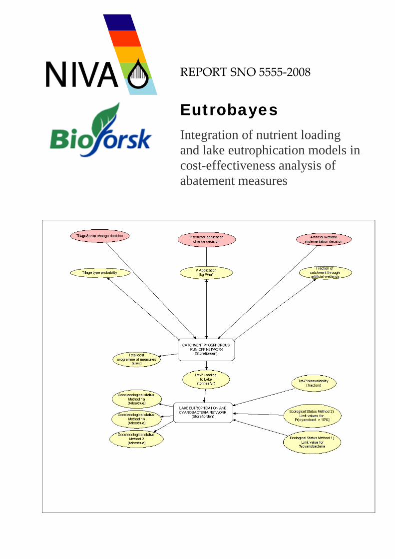
REPORT SNO 5555‐2008  

Eutrobayes Integration of nutrient loading and lake eutrophication models in cost-effectiveness analysis of abatement measures  

REPORTNorwegian Institute for Water Research – an institute in the Environmental Research Alliance of Norway

Main Office Regional Office, Sørlandet Regional Office, Østlandet

Regional Office, Vestlandet

Regional Office, Midt-Norge

Gaustadalléen 21 Televeien 3 Sandvikaveien 41 P.O.Box 2026 P.O.Box 1266 N-0349 Oslo, Norway N-4879 Grimstad, Norway N-2312 Ottestad, Norway N-5817 Bergen, Norway N-7462 Trondheim,

Norway Phone (47) 22 18 51 00 Phone (47) 22 18 51 00 Phone (47) 22 18 51 00 Phone (47) 22 18 51 00 Phone (47) 22 18 51 00 Telefax (47) 22 18 52 00 Telefax (47) 37 04 45 13 Telefax (47) 62 57 66 53 Telefax (47) 55 23 24 95 Telefax (47) 73 54 63 87 Internet: www.niva.no

Title

Eutrobayes Integration of nutrient loading and lake eutrophication models in cost-effectiveness analysis of abatement measures

Serial No.

5555-2008

Project number

26014

Date

September 2008

Pages

82

Author(s)

David N. Barton, Marianne Bechmann, Hans Olav Eggestad, Jannicke Moe, Tuomo Saloranta, Sakari Kuikka, Phil Haygarth

Topic group

Integrated water resources management

Geographical area

Norway

Distribution

Free

Printed

NIVA

Client(s)

Norges Forskningsråd (Research Council of Norway)

Client ref. EutroBayes (171692/S30) and Model SIP (172708/S30)

Abstract

Bayesian network methodology is used in the catchment of Storefjorden, South Eastern Norway, to integrate models of phosphorus (P) abatement costs and effects, as well as models of lake P and eutrophication dynamics. The Bayesian network integrated model was used to explore and evaluate the probable (and improbable) outcomes and uncertainties of (i) the eutrophication problem and (ii) the cost-effectiveness analysis of the corresponding abatement measures. In addition, factors which affect the reliability of transferring cost-effectiveness data for nutrient abatement measures between river basins were detected with a view to informing Norwegian implementation of the EU Water Framework Directive, and the relative uncertainty of model components within the Bayesian influence network was evaluated, with an aim to uncovering "information gaps" in abatement planning, and as a tool for prioritising future eutrophication research.

4 keywords, Norwegian 4 keywords, English

1. Tiltaksanalyse 1. Environmental Impact Assessment 2. Eutrofiering 2. Eutrophication 3. EUs Rammedirektiv for Vann 3. EU Water Framework Directive 4. Bayesianske nettverk 4. Bayesian belief networks

ISBN 978-82-577-5290-3

Tuomo Saloranta Project manager Øyvind Kaste Research manager Jarle Nygard Strategy Director

Eutrobayes

Integration of nutrient loading and lake eutrophication models in cost-effectiveness

analysis of abatement measures

NIVA 5555-2008

Preface

This report describes and summarizes much of the work done to develop Bayesian network models to study the eutrophication problem, its solutions and uncertainties in lakes in the EutroBayes and Model-SIP projects. These projects have provided us a marvellous opportunity to take some long leaps forward in the exciting and novel field of Bayesian modelling in environmental science. We would like to thank the Norwegian Research Council for funding for the EutroBayes (171692/S30) and Model SIP (172708/S30) research projects.

Oslo, September 2008

David N. Barton and Tuomo Saloranta

NIVA 5555-2008

ContentsPreface 3 Contents 4

Sammendrag 6 Overview of the EutroBayes Project 12

1. INTRODUCTION TO BAYESIAN NETWORKS 15

2. INTEGRATED MODEL 21

2.1 Lake Storefjorden and its catchment 21

2.2 Object oriented network for Lake Storefjorden catchment 22

2.3 Results – effectiveness and cost effectiveness of nutrient abatement measures 25

2.4 Sensitivity analyses 27 2.4.1 Interaction of abatement measures 30 2.4.2 Value of information analysis 31 2.4.3 Evidence sensitivity analysis using Hugin 33 2.4.4 Other examples of policy sensitivity analysis 35

3. LAKE EUTROPHICATION MODELS 39

3.1 MyLake eutrophication model 39 3.1.1 Model description 39 3.1.2 Model setup and results 39 3.1.3 Model sensitivity analysis 41

3.2 Cyanobacteria model 43 3.2.1 Model description 43 3.2.2 Data and discretisation 44 3.2.3 Results and sensitivity analysis 46 3.2.4 Assessment of ecological status: alternative approaches 46

4. NUTRIENT LOADING MODEL 49

4.1 Tillage and crop changes 51

4.2 Soil P content and P leaching 53

4.3 Artificial wetlands 54

4.4 Total catchment loading 55

5. NUTRIENT ABATEMENT COSTS 56

5.1 Tillage and crop changes 56

5.2 P-Application changes 56

NIVA 5555-2008

5.3 Artificial wetlands 58

6. STAKEHOLDER DEFINED CAUSE-EFFECT NETWORKS FOR ABATEMENT MEASURES 60

7. MODEL TRANSFERABILITY BETWEEN SITES 65

7.1 Lake Steinsfjorden and its catchment 66

7.2 Erosion risk 67

7.3 Crop distribution and management 68

7.4 Soil P status 68

7.5 Soil P application 69

7.6 Crop yields 70

7.7 Conclusions regarding transferability across catchments 70

8. DISCUSSION AND FUTURE RESEARCH QUESTIONS 72

9. CONCLUSION 76

10. REFERENCES 81

11. APPENDIX 1 83

12. APPENDIX 2 85

NIVA 5555-2008

Sammendrag

Tiltakseffektivitet og kostnadseffektivitet Hovedmålsetningen med EutroBayes1 prosjektet har vært å bruke såkalt Bayesiansk nettverk-metode til å integrere belastnings- og kostnadsmodeller for avbøtende tiltak for fosfor med en innsjømodell for prediksjon av fosfor-konsentrasjon og eutrofieringsdynamikk. Bayesianske nettverk er brukt for å vurdere sannsynlige (og usannsynlige) scenarier og usikkerhet i (i) eutrofieringseffekter, og (ii) kostnadseffektivitet av avbøtende tiltak. Videre har vi vurdert forhold som påvirker påliteligheten av å overføre kostnadseffektivitets-vurderinger mellom nedbørfelt. Dette er en relevant problemstilling i forbindelse med implementering av den nye Vannforskriften og EUs Vannrammedirektiv (VRD). Den integrerte nettverks-modellen ble også brukt til å avdekke informasjonsgap i tiltaksanalyse og identifisere behov for fremtidig forskning innen modellering av eutrofiering. Bayesianske nettverk er kraftige beregningsmodeller som utgjør intuitive og visuelle verktøy for a kombinere kvantitative informasjon fra mange ulike kilder i et felles rammeverk for tiltaksanalyse. Bayesianske nettverk beskriver sannsynlighetsbaserte - til forskjell fra deterministiske - sammenhenger mellom variable på tvers av ulike forklaringsmodeller. Med en nettverks-modell for Storefjordens nedbørfelt og innsjø (Morsa) har vi demonstrert hvordan vi kan beskrive kvantitativt ”risiko for ikke å nå god økologisk status”, eller alternative sannsynligheten for å nå god status (miljømålet i Vannforskriften og VRD). Vi har tatt for oss ett enkelt kriterie – cyanobacterie-forekomst – for å demonstrere prinsippet. Figure 9-1 viser det overordnede netteverket for tiltaksanalysen og dagens tilstand uten ytterligere tiltak. Figur 9-1. Nettverk som illustrerer dagens status uten tiltak

Merknad til Figur 9-1: variablene i nettverket vises med ellipser og årsak-virkning sammenhenger med piler mellom dem. Søylediagrammene viser sannsynlighetsfordelingene til hver variabel der det 1 Modelling EUTROphication with BAYESian networks

6

NIVA 5555-2008

første tallet er sannsynligheten og det andre tallene er tilstander (utrykket som intervaller eller enkeltverdier). Storefjorden er i “god status” med en sannsynlighet som varierer mellom 63 til 84.7%, avhengig av hvilken klassifiseringsmetode vi bruker for cyanobakterier. Dette er et eksempel på karakterisering av økologisk status som også fanger opp naturlig variasjon i vannforekomstens tilstand. I forbindelse med vurderingen av et handlingsprogram for vannområdet, ønsker man videre å kvantifisere kostnadseffektiviteten av ulike tiltak (redusert jordarbeiding, redusert gjødsling og fangdammer er tiltakene som ble vurdert.). Figur 9-2 viser det samme nettverket, men nå med implementering av tre tiltak (all høstpløying stoppes til fordel for stubb; reduksjon i gjødslingsnivåer til 0 ved P-Al tall over 15; økning av arealet som drenerer til fangdammer fra 23% til 30-50%). Effekten av denne tiltakspakken til sammen er å øke sannsynlighet av at Storefjorden er i ”god status” fra 63% til 73.5%, med andre ord en økning på litt over 10 %-enheter i sannsynlighet. Tiltakene som her vurderes er omfattende: om lag 2500 nye hektar under stubb i stedet for høstpløyd; mellom 700-2700 nye hektar som drenerer til fangdammer; en halvering av gjennomsnittelig gjødsling/hektar. I dette arbeidet har vi ikke vurdert hva nytten av en 10 %-enheter økning i sannsynligheten for god økologisk status vil si for brukere av Storefjorden. En tidligere studie av en annen tiltakspakke der man brukte en tidligere versjon av nettverksmodellen fant at tiltakskostnadene oversteg nytten i form av betalingsvillighet for vann som er egnet for rekreasjons- og drikkevannsformål (Barton et al. 2008). Figur 9-2. Nettverk som illustrerer økologisk status med en tiltakspakke

Hva er så kostnadseffektiviteten av de tre ulike tiltakene? Tabell 9-1 oppsummerer resultatene. Redusert gjødsling er det mest kostnadseffektive tiltaket da det har stor effekt og er antatt kostnadsbesparende. En besparelse på kr 1000 i fosfor kostnader2 resulterer i en reduksjon på 2.28 kg fosfor belastning av Storefjorden. Det er et ”vinn-vinn” tiltak. Redusert jordarbeiding er mer 2 Basert på en beregnet skyggepris for fosfor (se kapittel 5)

7

NIVA 5555-2008

kostnadseffektivt enn fangdammer. For disse siste to tiltakene er kostnadseffektiviteten flere ganger lavere enn beregninger som ble gjort i tiltaksanalysen for Morsa’s nedbørfelt (Lyche Solheim og andre 2001). Sistnevnte var en deterministisk studie som vurderte tiltakseffektivitet på ”optimale” arealer. Sammenligningsgrunnlaget med vår studie på ”gjennomsnittsarealer” er derfor ikke identisk. Målrettet bruk av tiltak i delnedbørfelt vil ha større kostnadseffektivitet enn den vi finner med vår nettverksmodell. Det illustrerer imidlertid poenget med at kostnadseffektivitet avhenger av variasjonen over de arealene man har med i tiltaksvurderingen. Tabell 9-1. Kostnadseffektivitet av tiltakene Tiltak:

Kostnadseffektivitet (lavt-høyt estimat) (reduksjon i kg Tot-P /tusen kroner) Lyche Solheim et al.(2001)

Forventet kostnadseffektivitet (reduksjon i kg Tot-P /tusen kroner) Denne studien

Kostnads-effektivitets-rangering

Redusert P gjødsling Ikke beregnet -2.28 1

Redusert jordarbeiding

4.00 - 11.11 1.14 2

Fangdammer 0.88 - 2.04 0.18 3

Note: redusert gjødsling er et kostnadsbesparende tiltak som gjør at kostnadseffektivitet vises som et negativt tall (positiv effekt delt på negative kostnader=negativ kostnadseffektivitet). På den andre siden har vi antatt at det er 100% tiltaksgjennomføring på årsbasis og uten forsinkelser eller andre kostnader enn utgifter til tiltaket og evt. redusert avkastning fra arealer. Vi har fått forvaltningen og andre interessenter til å sette opp egne konsekvens-nettverk som beskriver de sammenhengene de er mest opptatt av. Denne øvelsen - som omtales nærmere i kapittel 6 – avdekket et stort kunnskapsgap om betydningen av faktorer som betinger bondens implementering av tiltak. Dette temaet er ikke vurdert i vår modell. Tiltaksvurdering under Vannforskriften Vannrammedirektivet og den norske Vannforskriften krever at vannområder gjennomfører karakterisering av nedbørfelt som har som hovedmålsetting å vurdere risiko for at enkelt vannforekomster ikke når ”god økologisk status” og også beskrive et basisscenario som skal brukes i tiltaksvurdering (en fremskrivning av dagens bruksomfang og tilstand)3 . Veilederen går lite inn i betydningen av å dokumentere naturlig variasjon som en del av tilstandsbeskrivelsen, ei heller hvordan man skal forholde seg til og dokumentere usikkerhet. I tilfeller der naturlig variasjon er en tilstandsparameter i beskrivelsen av økologisk status, kan Bayesianske nettverk være et godt rammeverk for dokumentasjon (i form av sannsynlighetsfordelinger), som senere også kan brukes til vurdering av tiltakseffektivitet. Tiltaksprogrammet under Vannforskriften skal så vurderes i forhold til kostnadseffektivitet. Veilederen4 som er utviklet anbefaler lokale myndigheter som skal utføre det praktiske planarbeidet å vurdere tiltakseffektivitet kvalitativt ved hjelp av en skala på 3 nivåer som reflekterer konsekvens og omfang (p.21). I praksis anbefaler man også at tiltakseffektivitet vurderes på tiltakstedet (ved jordekanten, enden av røret) heller enn i vannforekomsten. Man erkjenner at dose-respons informasjon er mangelfull på lokalt nivå. Vurderingen av kostnadseffektivitet blir i den forstand en ekspertskjønnsbasert vurdering. Veilederen sier lite om metoder for å dokumentere dette skjønnet, for 3 “Metodikk for Karakterisering av Vannforekomster i Norge”. Versjon 1, 13.08.07 http://www.vannportalen.no/hoved.aspx?m=45147 4 ”Veileder i Arbeidet med Miljøtiltak”, Direktoratsgruppen, Versjon 1. 12.09.07 http://www.vannportalen.no/hoved.aspx?m=45149 )

8

NIVA 5555-2008

eksempel hvordan man skal vekte konsekvens per arealenhet (for eksempel redusert P belastning per hektar) med omfang (for eksempel antall hektar tiltaket gjennomføres over). Selv om dose-respons forhold er dårlig kjent skal forhold av relevans for kostnadseffektivitet så langt som mulig dokumenteres (s. 22, Tiltaksveileder):

Sesongvariasjon Forsinkelser i tiltakseffekt Avstand fra tiltakssteder til vannforekomsten Tidligere dokumenterte tiltakseffekter med overvåkningsdata Andre stedsspesifikke forhold

Denne rapporten viser at Bayesianske nettverk kan brukes til å dokumentere disse forholdene, både i form av ekspertskjønn eller der kvantitative data er tilgjengelig. Rapporten viser hvordan kvantitativ kostnadseffektivitetsrangering av tiltak kan gjøres med et ”blandet” datagrunnlag. Den mest sannsynlige anvendelsen av Bayesianske nettverk under Vannforskriften vil likevel kunne være i vurderinger av unntak fra miljømålet. Tiltaksveilederen anbefaler bruk av en stor feilmargin i vurderingen av om tiltakskostnadene er uforholdsmessig store i forhold til nytten av å nå god økologisk status. Videre anbefaler veilederen at tiltaks effektivitet bør vurderes som en del av tiltakspakker heller enn enkeltvis (s. 34). En vurdering av ”uforholdsmessighet” som samtidig også skal sikre store ”feilmarginer” nødvendiggjør en kvantitativ tilnærming. Bayesianske nettverk er også godt egnet til å håndtere effekten av flere tiltak samtidig, og spesielt tilfeller der effekten av noen oppstrømstiltak betinger effekten av andre nedstrømstiltak. I mangel av data om tiltaksnytte anbefaler tiltaksveilederen at man trinnvis vurderer miljømåloppnåelse ved å fjerne ett og ett tiltak fra tiltakspakken, der man begynner med det minst kostnadseffektive tiltaket og jobber seg bakover inntil man har nådd miljømålet. I denne rapporten demonstrerer vi hvordan Bayesianske nettverk kan gjøre slik ”bakover ressonering” lettere (kapittel 2). Vi svarer på spørsmålet, ’hvilket tiltaksnivå er nødvendig for å være sikker på at man når eller ikke når miljømålet?’ I programvaren Hugin kan en spesifisere en hvilket som helst sikkerhetsmargin som forvalterne ønsker å bruke i tiltaksvurderingen. Forskningsprosjektet EutroBayes har demonstrert et potentsiale for Bayesianske nettverk i kvantitative tiltaksanalyser. Hva vil kreves for å bringe Bayesianske nettverk fra forskningen over i anvendelse i forvaltningen? Denne rapporten gir noen indikasjoner på gap som fortsatt eksisterer: (i) risiko-kommunikasjon (ii) metodologisk usikkerhet (iii) tekniske begrensninger i programvare: (i) Risiko-kommunikasjon:

• Tiltakskostnader og effekter beskrives som sannsynlighetsfordelinger, noe som ofte oversettes til “usikkerhet”. Forskere kan gjøre en bedre jobb i å fokusere på hva vi vet og hvor sikkert det er. I denne studien fant vi for eksempel at sannsynligheten for at Storefjorden er i ”god status” økte fra 63% til 73.5% med en tiltakspakke. Vi ble 10 %-enheter sikrere om miljømålet med en tiltakspakke.

• ”Bayesianske nettverk” er et teknisk begrep som det ikke finnes noen god oversettelse for. Vi har brukt ”konsekvens-nettverk” i diskusjoner med forvaltningen og bønder. Man bør fokusere på at det er en metode for ”kvantitativ og integrert tiltaksanalyse”

(ii) Metodologisk usikkerhet:

• Nettverkene bruker sannsynligheter om miljøforhold i et bestemt nedbørfelt (for eksempel arealbruk, erosjonsrisiko, fosfor-nivåer i jorden). GIS data om romlig fordeling av slike forhold er en forutsetning for at man skal gjøre en korrekt analyse. I noen tilfeller mangler slike data (for eksempel på fordelingen av P-Al tall) noe som gjør at sannsynlighetsfordelingene for gjødslingstiltak ikke blir korrekte (med andre ord man beregner mer variasjon/usikkerhet enn det som faktisk finnes ved ikke å arealvekte dataene).

9

NIVA 5555-2008

• Nettverket vårt for tiltakseffekt og –kostnader antar at tiltak implementeres 100% i utvalgte

arealer. Man antar at kostnader er forbundet med tekniske tiltak og eventuelt tap i avling, men ikke at det finnes andre implementeringskostnader, eller at visse gårder velger ikke å implementere tiltak. Dette gjør samtidig at forventet kostnadseffektivitet i tiltakene overestimeres, og usikkerheten ved effekt underestimeres. Dette er ikke et problem for rangering av tiltak så lenge manglende implementering straffer tiltakene likt. Det er imidlertid et problem i forhold til vurdering av miljømåloppfyllelse, og vurderingen av uforholdsmessighet i tiltakskostnadene. Fremtidige scenarie-analyse må derfor jobbe med hvilke forhold som påvirker implementeringsgraden av ulike tiltak hos aktørene (for eksempel juridiske og finansielle insentiver).

• Innsjø-modellen var forenklet for å kunne raskt gjøre simuleringer som danner grunnlaget for

sannsynlighetsfordelingene av fosfor-konsentrasjoner, algebiomasse og forekomst av blå-grønnalger. Modellen av planktonsamfunn tok ikke høyde for populasjonsdynamikk, ei heller rollen til nitrogen som mulig næringsbegrensning. Dette medfører at variabilitet i cyanobakterie-nivåer muligens er underestimert.

• I denne rapporten har vi illustrert vurdering av ”god økologisk status” på ett enkelt

kvalitetselement (blågrønnalger). I praksis vil økologisk status bli definert av flere kvalitetselementer og støtteparametre (makroinvertebrater, fytoplankton, fytobentos, macrofyter, makroalger, angiosperm, fisk, kjemisk vannkvalitet). Dette kompliserer vurderingen av risiko for ikke å nå ”god status”, spesielt når spørsmålet om uforholdsmessighet skal vurderes. Det kan for eksempel være interaksjoner mellom de ulike kvalitetselementene, eller at ulike tiltak har ulike effekt på ulike kvalitetselementer (for eksempel effekten av geomorfologiske tiltak versus forurensningstiltak på alger versus fisk). Bayesianske nettverk gir et metode-rammeverk for å vurdere slike samspillseffekter.

(iii) Tekniske begrensninger

• Kausale nettverk må defineres for en gitt tidsperiode. De egner seg best for

miljøproblemstillinger der tiltakseffekter gjør seg gjeldende i løpet av ett år (bakteriologisk forurensning, eutrofiering, akutt forurensning og opprydding). Kausale nettverk egner seg mindre godt til å analysere dynamiske forhold i flerperiode systemer da feed-back effekter er vanskelige å modellere. Dette gjør dem i utgangspunktet mindre egnet til studie av persistent forurensning som miljøgifter.

• Kausale nettverk må defineres for et gitt geografisk område. For at sannsynligheter om miljøforhold skal beregnes på en sammenlignbar måte, må de ulike datakildene gjelde det samme geografiske området. I praksis kan dette være vanskelig i store nedbørfelt med mange kommuner med ulik praksis for overvåkning. En mulig løsning er å lage flere netteverk som er koblet sammen.

• Sannsynlighetsfordelinger som beskriver naturforhold vil ofte måtte angis som intervaller (”diskrete fordelinger”), for eksempel at sannsynligheten for fosfor-konsenstrasjon ligger i et intervall på 20-25, 25-30, 30-35 mg/m3 etc. Dette fordi vi mangler detaljert nok data på årsakene (i dette tilfellet P-belastning). Hvilke intervaller sannsynlighetsfordelingene deles opp i kan ha avgjørende betydning for beregningen av tiltakseffektivitet. Det krever at fordelingene er godt dokumenterte og vurderes i følsomhetsanalyser.

Hovedalternativet til Bayesianske nettverk i kostnadseffektivitetsanalyse av tiltak er regneark som Excel® (e.g. Lyche Solheim et al. 2001). Alle begrensningene som er nevnt ovenfor gjelder også for regneark (med unntak av problemet med diskretisering av sannynlighetsfordelinger). Imidlertid har regneark som Excel tre ulemper i forhold til Bayesianske nettverk slik de er anvendt i for eksempel Hugin Expert®: (i) regneark tar ikke hensyn til variabilitet med mindre de brukes sammen med simuleringsverktøy som for eksempel @Risk; (ii) de visualiserer ikke de kausale sammenhengene i

10

NIVA 5555-2008

modell-strukturen, regnearket er en ”svart boks” for utenforstående, (iii) regneark kan ikke brukes til ”induktiv” ressonering (for eksempel for å svare på spørsmålet, hva er sannsynligheten for ulike gjødslingsnivåer ig jordbruket gitt en observert forsfor-konsentrasjon i innsjøen?). Vi som har deltatt i EutroBayes prosjektet tror dette er tre viktige grunner til å anvende Bayesianske nettverk i kvantitativ konsekvensanalyser under Vannrammedirektivet.

11

NIVA 5555-2008

Overview of the EutroBayes Project

Bayesian network methodology provides a powerful, intuitively and visually appealing tool for combining (uncertain) information from different sources into a common framework and for analysing this particular system’s functioning and characteristics. Bayesian networks utilise probabilistic, rather than deterministic, expressions to describe relationships among variables. In a Bayesian network the system is represented as a directed graphical model, in which the subsystems (i.e. variables) are represented by nodes and the causal interactions between the variables by arrows linking the particular nodes (Figures 1-3). Each dependence indicated by an arrow represents a conditional probability distribution (in form of a discrete “conditional probability table”, CPT) that describes the relative likelihood of each value of the down-arrow node, conditional on every possible combination of values of the parent nodes. The principal project objective of the EutroBayes project was to use Bayesian network methodology in the two case study river basins, Storefjorden and Steinsfjorden, to integrate models of phosphorus (P) abatement costs and effects, as well as models of lake P and eutrophication dynamics. Due to time and data limitations the project established a full model only for the Storefjorden catchment. The Bayesian network integrated model was used to explore and evaluate the probable (and improbable) outcomes and uncertainties of (i) the eutrophication problem and (ii) the cost-effectiveness analysis of the corresponding abatement measures. In addition, factors which affect the reliability of transferring cost-effectiveness data for nutrient abatement measures between river basins were detected with a view to informing Norwegian implementation of the EU Water Framework Directive, and the relative uncertainty of model components within the Bayesian influence network was evaluated, with an aim to uncovering "information gaps" in abatement planning, and as a tool for prioritising future eutrophication research. In the project we have, according to the goals set, used the Bayesian network methodology to successfully integrate models of P abatement costs and effects with lake P and eutrophication dynamics (the MyLake model). The finished product, Bayesian network integrated models for Storefjorden catchment, formulated in the Hugin software (www.hugin.com), can now be used to explore and evaluate the outcomes of different abatement measures in a probabilistic way, for example the question of what the probability of achieving a good lake status (defined as the fraction of cyanobacteria < 10% of the total algae biomass in June-September) will be after a certain abatement measure has brought the lake into a new quasi-steady state. Among the factors which most affect the reliability of the abatement cost-effectiveness data transfer between river basins are assumptions about (i) cyanobacteria limit values, (ii) bioavailable P fraction, (iii) tillage and cropping patterns, (iv) fertiliser application recommendations, and (v) effectiveness of artificial wetlands. The largest "information gaps" in abatement planning were related to (i) modelling the effect of altered fertiliser application over time on soil P concentrations, (ii) the effect of changed tillage practices for other crops than wheat, and (iii) changes in crop yield and production costs due to changing tillage and fertilisation practices. Our modelling of alternative approaches to evaluating lake status based on chemical and biological parameters also reflects continued uncertainty at the policy level regarding an operational definition of good ecological status in the Water Framework Directive. In the EutroBayes project we have shown that Bayesian networks can successfully be used to evaluate the ‘disproportionate cost’ issue posed by the EU Water Framework Directive. The most common nutrient mitigation measures (reduced tillage practices, reduced fertiliser application, and artificial wetlands) had, however, in our case a relatively diffuse effect on lake water quality when uncertainty in the models, data and expert opinion underlying the driver-pressure-state-impact chain is modelled explicitly in a Bayesian networks and influence diagrams. Although it is possible that the “smearing” of the effect of the abatement measures downstream in the river basin in the Bayesian network might still be partly due to non-optimal model design, we strongly believe that this vague response is mainly a result of explicitly modelling the uncertainty underlying the complicated biogeochemical river basin system and the effect of abatement measures carried out over a variable landscape. Consequently, the

12

NIVA 5555-2008

Bayesian network may well help us to understand why measures don't seem to work as the high variability in the river basin system may mask or "buffer" their effect. The relatively lacking effectiveness of the programme of measures may, however, be counter-intuitive to managers used to working on deterministic models. This underlines the point that the integrating and multi-disciplinary process of defining a network, determining its probability distributions and conducting sensitivity analysis may be more important than the results of the analysis itself. The Bayesian network for Storefjorden catchment was quality controlled and errors were spotted by an external reviewer in a matter of a few hours, showing that a Bayesian network can portray a complex management problem in an easily accessible fashion. While we see Bayesian decision analysis as an important addition to river basin managers’ toolbox, we feel that further work must be done on the limitations before Bayesian networks can gain wider appeal in management of water resources. These limitations include: (i) discretisation, i.e. that relative to a continuous probability function, there is some information loss at each node due to discretisation assumptions; (ii) steady-state assumption, i.e. that dynamic time-dependent models are difficult and laborious to build in form of a Bayesian network; (iii) difficulties in assuring the spatial and temporal consistency of probability distributions across a number of models, datasets and expert judgments from different disciplines; (iv) hidden correlation of assumed unconditional probability distributions through catchment-wide processes (e.g. rainfall), leading to overestimation of uncertainties, (v) limitations on modelling dynamic feedback effects on land-uses over the multi-annual period under consideration (2005-2015; this was particularly problematic in determining the interaction between fertilisation practices and the store of soil-P). The reported advantages of Bayesian networks in promoting integrated/inter-disciplinary evaluation of uncertainty in integrated river basin management, as well as the apparent advantages for risk communication with stakeholders, are also moderated in our case by the cost of obtaining reliable probabilistic data. The most central research tasks in the EutroBayes project have been:

• Sharing and learning the Bayesian network modelling skills in numerous project meetings and expert workshops (NIVA, Univ. Helsinki).

• Building a river basin model for estimating the effects of different nutrient abatement measures in the river basin on the total P load. This model has been built to be rather general so that it can easily be transferred between different river basins (Bioforsk, IGER).

• Using the MyLake model for simulating the effect of the total P load into lakes Vansjø-Storefjorden and Steinsfjorden on the total P and chlorophyll concentration in the lake water. The model was also thoroughly analysed for its sensitivity to different parameters, and adapted for simulating metalimnetic algae populations in Steinsfjorden (NIVA).

• Constructing empirical models by using data from all counties of Norway (in total 1326 samples). These models were relating water temperature as well as the total P and chlorophyll concentration in the lake water to the proportion of cyanobacteria of the total algae biomass in the lake. Three different modelling methods were tested and assessed. The proportion of cyanobacteria was used as indicator for lake status in Vansjø-Storefjorden. In lake Steinsfjorden chlorophyll was used as indicator for lake status due to deeper subsurface cyanobacteria population (NIVA).

• Discussing and defining suitable interfaces, in terms of spatiotemporal resolution, variable selection and discretization, in order to couple the three submodels of the three river basin domains (soil and runoff system, lake chemistry, lake biology) into one functioning network (NIVA, Bioforsk, IGER, Univ. Helsinki).

• Addressing different uncertainties which affect the credibility and reliability of the results emerging from the integrated Bayesian network (NIVA, Bioforsk, IGER, Univ. Helsinki).

• Involving stakeholders in the design and evaluation of the Bayesian network models in two meetings arranged in the county of Østfold where the Lake Vansjø-Storefjorden is located (NIVA, Bioforsk).

13

NIVA 5555-2008

• Identifying available data on costs of nutrient abatement measures across the cropping systems and agronomic practices that are relevant for highly eutrophic catchments in Norway, and which are expected to be the focus of programmes of measures under the Water Framework Directive (NIVA, Bioforsk, IGER).

• Evaluating alternative approaches to cost-effectiveness analysis under uncertainty made possible by Bayesian belief networks (NIVA).

The major sources of uncertainty in the models and the gaps in our knowledge were identified by different sensitivity analysis techniques, as well as by qualitative discussions. The simple Monte Carlo simulation based uncertainty analysis approach used with the lake model will provide a straightforward and easy way to propagate some specific parameter uncertainties into the nutrient abatement scenario results. However, a Markov chain Monte Carlo based technique might in the future be preferred for combined model calibration and uncertainty analysis. This technique is well-suited for tracing and quantifying the extent of confounding parameter identification (i.e., different parameter value combinations may produce the same model result), parameter correlations and uncertainties, although its application in practise may be more time- and skill-demanding. For the other models, expert judgement and statistical analysis were used for quantification of uncertainties. It is good to bear in mind, however, that the quantification of uncertainties will always remain uncertain in itself. For example, the fact that the lake model cannot itself simulate shifts in the composition of the phytoplankton community, or that population dynamics of the phytoplankton-predating species (or the food web in general) are not simulated in the model, represent methodological model uncertainties, which are not captured in the Monte Carlo simulations. Thus, we have also considered during the project the more qualitative expressions of uncertainties, as well as the detection of problems where uncertainty can and cannot be reduced, whether the variability/uncertainty is too large for a model to be useful, or the contrary, whether a simpler model would also be less "honest". The work with using the Bayesian networks in integrating models for uncertainty analysis and risk assessment will continue in other ongoing projects, notably NIVAs Strategic Institute Programme (SIP) on Modelling.

14

NIVA 5555-2008

1. Introduction to Bayesian Networks

In this section we give a short introduction to Bayesian Networks, and briefly explain their extension to decision analysis in what is known as Influence Diagrams. We also explain the meaning of an “object-oriented Bayesian network” (OOBN). Object-oriented Bayesian networks are used through the report to conduct impact analysis and cost-effectiveness analysis. Figure 1-1 illustrates both a Bayesian network and an influence diagram in the context of a generic driver-pressure-state-impact model, for example for water quality management (Barton et al. 2008). In this stylised example the management context is made up of the states of an exogenous variable X conditioning water quality state S, and the decision D on whether the pressure P mitigating measure is implemented or not. In this framework prior knowledge of water quality could be expressed as probability of a state S given pressure P and exogenous variable X: Pr (S | P, X); similarly probability of nutrient loading pressure P dependent on the decision D : Pr (P | D). In an impact analysis a manager may be interested in determining the posterior probability for a state given a pressure and the states of context variables c=c(D,X): Pr (S | P , c), or conversely a likelihood, expressed as a probability of pressure given a state given context variables: Pr (P | S , c). Figure 1-1. A graphical definition of Bayesian Networks and Influence Diagrams in a Driver-Pressure-State-Impact modelling framework

Source: Barton et al. 2006. Note: Prior knowledge: Probability of water quality state S: Pr(S); Probability of nutrient loading pressure P: Pr(P). Posterior: Probability of a state given a pressure: Pr( S | P). Likelihoods: Probability of pressure given a state: Pr (P | S) Bayes’ rule (eq.1) expresses the relationship between the prior, likelihood and posterior probabilities in the network.

(1) )|Pr(

)|Pr(),|Pr(),|Pr(cP

cScSPcPS ×=

15

NIVA 5555-2008

Whereas a BN is a model for reasoning under uncertainty, an influence diagram (ID) is a probabilistic network for reasoning about decision-making under uncertainty (Kjærulff and Madsen, 2005). The focus of the EutroBayes was on cost-effectiveness analysis, where cost and effectiveness outcomes are measured with different units, i.e. on different (utility) scales, as opposed to cost-benefit analysis (CBA) where outcomes are measured in monetary units. Cost and benefit outcomes can be expressed as utilities, making Influence diagrams well suited for CBA For an example of benefit-cost analysis using Influence Diagrams see Barton et al. (2006, 2008). We used the commercially available software called Hugin Expert® (www.hugin.com) to implement the Bayesian calculus shown in equation (1).

Bayesian networks are made of a series of chance nodes which are expressed as conditional probability tables (CPTs) that are linked together in cause-effect chains (Figure 1-2). A CPT is a ”response surface” representing data correlations, model simulations or expert opinion regarding the relationship between input (causes) and an output (effect) variables. Bayesian networks (without decision and utility nodes) are sufficient for evaluating cost-effectiveness issues. However, a brief explanation of Influence Diagrams is as follows. Referring back to the generic influence diagram in Fig. 1-1, the software depicts decision nodes as rectangles (exogenous policy drivers). Utility nodes representing impacts of decisions (costs and benefits) are

depicted as diamonds. Chance nodes (ovals) are used to depict exogenous variables described by unconditional probability distributions, as well as endogenous variables described by joint probability distributions conditional on the states of one or more parent nodes. Influence diagrams with decision and utility nodes estimate expected (net) utility of decisions accounting for all probability distributions of the network.

Figure 1-2. Conditional probability table

Note: CPT is a ”response surface” representing data correlations, model simulations or expert opinion regarding the relationship between input (causes) and an output (effect) variables.

Conditional probability distributions (CPT) are displayed in a particular way in the Hugin Expert® software we use to structure the analysis. Figure 1-3 shows two examples of probability distributions used in the model in this report. The upper panel A shows the probability of finding different tillage land use types in the catchment. This is based on geographical information system (GIS) calculation of relative areas of each land use type. The distribution basically says that if you picked a random hectare in the Storefjorden catchment there would be a 45.04% chance that it would be managed as stubble during the winter. Lower panel B shows an discrete distribution of erosion at plot level. It reads as follows; there is a 50.8% chance of erosion risk lying between 0-500 kg suspended solids per hectare per year (kg SS/ha yr).

Figure 1-3A. Example of a categorical probability distribution of different tillage land use types

Figure 1-3B. Example of a discrete probability distribution of erosion at plot level

16

NIVA 5555-2008

A discrete distribution splits a continuous variable into intervals, showing that we have limited information (there is uncertainty about) the exact nature of erosion within each interval. A continous distribution withouot intervals contains the most information, but is also the most computationally heavy to handle in a model. In this report we use either categorical or discrete distributions as shown in Figure 1-3. Figure 1-4 shows how probability distributions are conditional within a network. The probability distributions in the network are illustrated next to its respective variable, so-called network “nodes”. We see that ‘erosion’ at plot level is conditional on C-factors5, Soil Erosion Risk factor (KLS) and precipitation R-factor. The erosivity or C-factors are conditional in turn on the land use type, which is in turn conditional on tillage and crop change decisions (whether to implement a particular tillage policy or not). This little network in fact illustrates the so-called Universal Soil Loss Equation (USLE) for the Storefjorden catchment. Figure 1-4. Example of a Bayesian network where erosion risk is a probability distribution conditional on C-factors, Soil Erosion Risk factor (KLS) and precipitation R-factor.

The “e” on the ‘Tillage&crop change decision’ node shows that the network has been given ‘evidence’ stating that we are looking at a scenario with “no measures”, i.e. the current land use situation. Throughout this report we use “object-oriented Bayesian networks” (OOBNs) (Figure 1-5). Hugin Expert can be used to organise several different sub-networks representing different model simulations, data-correlations and expert judgement (erosion risk modelled in Figure 1-4 could be such a sub-network). Uncertain processes are described in the form of CPTs which are organised in Bayesian Networks, which in turn are organised as objects in a hierarchy. The whole hierarchical problem structure is called an Object-Oriented Bayesian Network (OOBN). 5 C: cover and management factor. K: soil erodability factor. LS: topographic factor. R: erosivity of rain factor

17

NIVA 5555-2008

Figure 1-5. Object-oriented Bayesian network (OOBN)

Source: Barton et al. 2006.

18

NIVA 5555-2008

Figure 1-6. Example of an object oriented bayesian network (OOBN) in Hugin. The nodes “Catchment phosphorus run-off network” and “Lake eutrophication and cyanobacteria network” (shown here) are sub-networks illustrated as white rectangles.

Evaluating Bayesian networks A number of different sensitivity and scenario analyses can be performed in Bayesian networks using the Hugin Expert functionality. Some of these will be illustrated in this report.

• Number of variables

o One variable at a time – this is the “traditional” approach to sensitivity analysis often seen in e.g. Excel models

o Several variables at a time – this is also known as “scenario analysis”

• Direction of reasoning

o Deductively – this is a “top-down” analysis where causal factors are adjusted and the result on effect variables is evaluated

o Inductively – this is “bottom-up” analysis where effect variables are adjusted and the

required values in causal variables is evaluated

• Method

19

NIVA 5555-2008

o Manually – the use adjusts the probability values of the variables as desired, one by one or in groups

o Value of information analysis tool in Hugin - given a Bayesian network model and a

hypothesis variable, the task is to identify the variable, which is most informative with respect to the hypothesis variable.

o “Evidence sensitivity analysis” tool in Hugin.

o “Parameter sensitivity analysis” tool in Hugin (Parameter sensitivity analysis is

disabled for influence diagrams and OOBNs, so this tool cannot be used with our models.)

20

NIVA 5555-2008

2. Integrated model

2.1 Lake Storefjorden and its catchment The catchment draining to Lake Storefjorden via the Hobøl River is somewhat smaller than the whole Morsa catchment shown in Figure 2-1, which also includes a sub-catchment draining locally to Vestre Vansjø Lake. The Bayesian network focuses on the part of the Morsa catchment draining to Lake Storefjorden. It comprises a total cultivated area of 10285 hectares and a non-cultivated area of 50215 hectares. In the network the cultivated area is subject to nutrient abatement measures while the non-cultivated area contributes with a background nutrient loading. The Morsa catchment has been the site of many years environmental monitoring and a comprehensive study of municipal and agricultural abatement measures which in many ways is the precursor to the present study using Bayesian networks (Lyche Solheim et al. 2001). One advantage of the Morsa catchment is the close proximity to Skuterud, one of the so-called JOVA-sites for permanent monitoring of agricultural practices and run-off. Figure 2-1. Lake Storefjorden and Vestre Vansjø catchment (Morsa)

Note: The area immediately to the north of Moss town and Lake Vestre Vansjø is outside Lake Storefjordens sub-catchment.

21

NIVA 5555-2008

2.2 Object oriented network for Lake Storefjorden catchment Figure 2-2 shows the integrated object oriented Bayesian network for ecological lake status. The different components of the model are explained in greater detail in subsections further below. Figure 2-2. The integrated object oriented Bayesian network for ecological lake status.

Note: The structure of the Bayesian network integrated model for Lake Storefjorden catchment. In a Bayesian network the system is represented as a directed graphical model, in which the subsystems (i.e. variables) are represented by nodes, and the causal interactions between the variables by arrows linking the particular nodes. Each dependence indicated by an arrow represents a conditional probability distribution (in the form of a discrete “conditional probability table”, CPT) that describes the relative likelihood of each value of the node at the end of the arrow, conditional on every possible combination of values of the parent nodes. The network in Figure 2-2 provides an overview of selected unconditional nodes that may be catchment specific, the underlying sub-networks, and the conditional nodes showing policy relevant results such as whether “good ecological status” is attained and the “total cost of the programme of measures”.

22

NIVA 5555-2008

This is the most aggregated level of the model displaying only the main drivers – decisions to implement different nutrient loading abatement measures and the resulting distributions of tillage types, phosphorus fertiliser application and fraction of the catchment run-off being treated by artificial wetlands. The “catchment phosphorus run-off network (Storefjorden)” is an underlying network in the hierarchy which is driven by the aforementioned remediation decisions. This underlying network summarises expert knowledge and empirical models of phosphorus run-off processes in the Morsa catchment draining into Lake Storefjorden (the model for Lake Steinsfjorden is shown in appendix). Two main results are derived from this underlying network, namely the “total cost of the programme of measures” and the “tot-P loading to Lake”. The latter is a truncated distribution with a range from 5 to 30 tonnes tot-P/year. The truncation reflects the historical range of nutrient loading to Storefjorden which drives the underlying “lake eutrophication and cyanobacteria network (Storefjorden)”. The truncation is highlighted here to reflect that the range and discretisation of probability distributions in Bayesian networks are assumptions behind the model which are not visible in the graphical user interface shown above. The “lake eutrophication and cyanobacteria network (Storefjorden)” calculates the probability of “good ecological status” following three different methods (lower left hand Figure 2-2). Along with Tot-P loading, assumptions about Tot-P bioavailability, and limit values at which to evaluate good ecological status are shown (lower right hand Figure 2-2).

23

NIVA 5555-2008

Figure 2-3. Nutrient loading model for three different nutrient abatement measures showing their interaction

Note: The structure of the catchment runoff network depicted previously as a sub-network node in Figure 2-2. This network in turn contains sub-networks for costs of individual measures. This object-oriented Bayesian network modelling structure means that sub-networks can easily be replaced when new problem structures and data are used. Nodes encircled in solid grey lines are output nodes transmitting information to another network, nodes encircled in dashed grey lines are input nodes receiving information from another network.

24

NIVA 5555-2008

2.3 Results – effectiveness and cost effectiveness of nutrient abatement measures Cost-effectiveness has to be calculated outside the current network. For an example of a network where cost-effectiveness and benefit-cost analysis are conducted within the network see (Barton et al. 2008). The upper part of Figure 2-4 shows that the measures are set6 to the state “no measures”. The distributions under “tillage type probability”, “P Application” and “Fraction of catchment through wetlands” show the current situation as observed in Storefjorden Lake’s catchment today. Distributions further down show the resulting nutrient loading water quality and ecological status based on alternative methods of classification. The network shows quite a wide distribution for Tot-P loading to the lake Storefjorden in the status quo, but with a mean(μ) of 17,9 tonnes Tot-P/year (variance σ2= 67.9). This is around 0,5 tonnes Tot-P/year above the calibrated MyLake model values. This small deviation from observed mean nutrient loading may be due to the distribution having been truncated at 5 and 30 tonnes Tot-P/year. Truncation was carried out in order to fit the range of nutrient loadings from the abatement measures with the range of situations the MyLake model was simulated for . Figure 2-4. Network illustrating “no measures” or status quo probabilities

What is the ecological status of Lake Storefjorden today as it might be described in a River Basin characterisation report under the Water Framework Directive? Basing ecological status only on the cyanobacteria criteria (for demonstration purposes), Storefjorden is likely in “good status” with probabilities ranging from 63% to 84,7% depending on the classification method chosen. There is a 35,6% probability of Tot-P loadings above 25 tonnes Tot-P/year, and a 25,7 % probability of Tot-P loadings below 10 tonnes Tot-P/year. This is higher than the variance of monitored Tot-P loadings, because uncertainty regarding the effectiveness of measures under alternative scenarios is 6 The technical jargon is that evidence is “instantiated” in the network

25

NIVA 5555-2008

also reflected in the status quo situation. Note also that neither fixed value of R-bio, nor limit values for calculating the probability of good ecological status based on cyanobacteria probabilities have been assumed. Figure 2-5 illustrates the effects of implementing a proposed package of measures. The measures are illustrated in the three probability distributions at the top of the figure. Amongst others, the area under stubble is increased at the expense of autumn ploughing. Fertilisation intensity is reduced. The proportion of catchment run-off passing through wetlands is increased from 23% to somewhere between 30-50%. The effect of these measures is to increase the probability of good status from 63% to 73.5% (Method 2). Figure 2-5. Network illustrating a scenario “with measures”

The message of this sensitivity analysis of ecological status (Figure 2-5) is quite clear. Reduced fertiliser application is the most effective in reducing P-loading and increasing the probability of good status, as well as being a cost-saving measure.

26

NIVA 5555-2008

Reduced fertiliser application is the most effective in reducing P-loading and increasing the probability of good status, as well as being a cost-saving measure. A saving of kr. 1000 in P input costs7 results in a reduction of 2.28 kg of P loading to Storefjorden and is a “win-win” measure. Reduced ploughing measures is more cost-effective than artificial wetland construction relative to tot-P loading (Table 9-1). Cost effectiveness is shown to be much lower for reduced tillage and artificial wetland than in the most recent impact assessment from the catchment using a deterministic approach (no uncertainty) (Lyche Solheim et al 2001). Table 9-1. Cost-effectiveness of measures Measure Low-high estimate

effect/cost (reduction kg Tot-P /thousand kroner) Lyche Solheim et al 2001 (p.68)

Expected effect/cost (reduction kg Tot-P /thousand kroner) This study

Expected effect/cost (Increased % probability of good ecological status)/ million kroner This study

Cost-effectiveness ranking This study

Reduced fertiliser use

n.a. -2.28 -5.08 1

Reduced tillage 4.00 - 11.11 1.14 2.53 2

Artificial wetlands alone

0.88 - 2.04 0.18 0.41 3

Note: reduced fertiliser use is a cost-saving measure for reducing Tot-P loading(positive effect divided by negative costs). An analysis of different abatement measure packages showed that the cost-effectiveness of wetlands is 1/3 as great when implemented in combination with other measures which reduce upstream nutrient loading at source/in-field. Another way of looking at cost-effectiveness in Table 8.1 in the recipient is to look at the increase in probability that the water body will be of “good ecological status” per million kroner spent on abatement. In the case of reduced tillage a million kroner in increased tillage costs for farmers will result in a 2.53 % increase in the probability of good status, while for artificial wetlands a million kroner in increased costs results in an increased probability of good status by half a percent. The results in Table 9-1 should be read as indicative of what kind of analysis is possible with Bayesian networks rather than as the final word on relative cost-effectiveness of measures. The figures shown are means for the whole catchment and hide a lot of site specific variation, i.e. the ranking of reduced tillage and wetlands measures may be reversed in specific sites. 2.4

Sensitivity analyses In this section we illustrate inductive sensitivity analysis of ecological status (Figure 2-6a and b). The possibility to conduct inductive analysis is a feature Bayesian networks which is not possible to carry out in e.g. spreadsheet models. We also illustrate the “value of information” analysis tool which, amongst others, gives a ranking of the information in each node in the model relative to a so-called hypothesis variable, in this case “good ecological status”.

7 Using a computed shadow price for phosphate (see chapter 5)

27

NIVA 5555-2008

28

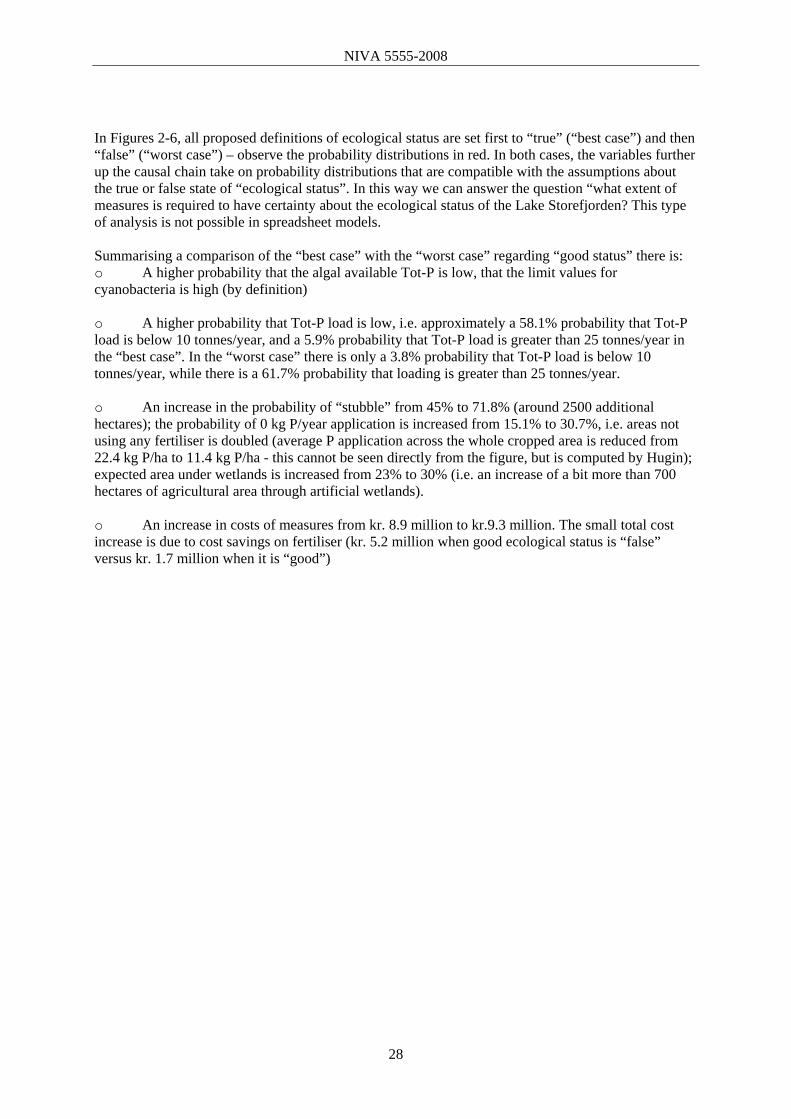
In Figures 2-6, all proposed definitions of ecological status are set first to “true” (“best case”) and then “false” (“worst case”) – observe the probability distributions in red. In both cases, the variables further up the causal chain take on probability distributions that are compatible with the assumptions about the true or false state of “ecological status”. In this way we can answer the question “what extent of measures is required to have certainty about the ecological status of the Lake Storefjorden? This type of analysis is not possible in spreadsheet models. Summarising a comparison of the “best case” with the “worst case” regarding “good status” there is: o A higher probability that the algal available Tot-P is low, that the limit values for cyanobacteria is high (by definition) o A higher probability that Tot-P load is low, i.e. approximately a 58.1% probability that Tot-P load is below 10 tonnes/year, and a 5.9% probability that Tot-P load is greater than 25 tonnes/year in the “best case”. In the “worst case” there is only a 3.8% probability that Tot-P load is below 10 tonnes/year, while there is a 61.7% probability that loading is greater than 25 tonnes/year. o An increase in the probability of “stubble” from 45% to 71.8% (around 2500 additional hectares); the probability of 0 kg P/year application is increased from 15.1% to 30.7%, i.e. areas not using any fertiliser is doubled (average P application across the whole cropped area is reduced from 22.4 kg P/ha to 11.4 kg P/ha - this cannot be seen directly from the figure, but is computed by Hugin); expected area under wetlands is increased from 23% to 30% (i.e. an increase of a bit more than 700 hectares of agricultural area through artificial wetlands). o An increase in costs of measures from kr. 8.9 million to kr.9.3 million. The small total cost increase is due to cost savings on fertiliser (kr. 5.2 million when good ecological status is “false” versus kr. 1.7 million when it is “good”)

NIVA 5555-2008

Figure 2-6a. Sensitivity analysis of ecological status (Storefjorden) “Best case” for ecological status

Figure 2-6b. Sensitivity analysis of ecological status (Storefjorden) “Worst case” for ecological status

29

NIVA 5555-2008

2.4.1 Interaction of abatement measures What is the effectiveness of measures alone and in combination? The Bayesian network can be used to evaluate this question. Figure 2-7 shows the nutrient loading network. We will evaluate the node “Particulate P” under different scenarios for implementation of artificial wetlands. The effects of the different combinations of measures are presented in Figure 2-8. While the effects of wetlands on nutrient loading are small both alone and in combination with other measures, they are clearly greater when implemented alone. The cost-effectiveness of wetlands will therefore be lower than what is suggested in table 2-1 because it is a “downstream” measure. Figure 2-7. Evaluating the effectiveness of artificial wetlands alone and in combination with reduced fertiliser and tillage practices using the nutrient loading network

Note: The effectiveness of artificial wetlands on particulate P loading is evaluated by looking at the decision nodes for the measures and the nodes “Particulate P(Out)” Figure 2-8. Results: Evaluating the effectiveness of artificial wetlands alone and in combination with reduced fertiliser and tillage practices. Baseline wetland (23% of

cultivated areas draining through artificial wetlands):

Wetlands implemented alone (30-50% of cultivated area through wetlands):

Mean effectiveness of wetlands on net nutrient loading

Effectiveness of wetlands alone

δμ= 0.15 kg P /ha

Only other measures implemented (no additional wetlands):

Wetlands implemented with other measures:

Effectiveness of wetlands in combination with other measures

δμ =0.05 kg P /ha

30

NIVA 5555-2008

2.4.2 Value of information analysis Consider the situation where a decision maker has to make a decision based on the probability distribution of a hypothesis variable (Hugin Expert 6.9 Manual). Prior to deciding on a remediation measure the decision-maker may have the option to gather additional information about the cost and effectiveness of the measure such as through additional monitoring, modelling or experiment. Given a range of variables for which one may gather information, which option should the decision-maker choose? That is, which of the given options will produce the most information? These questions can be answered by a value of information analysis.

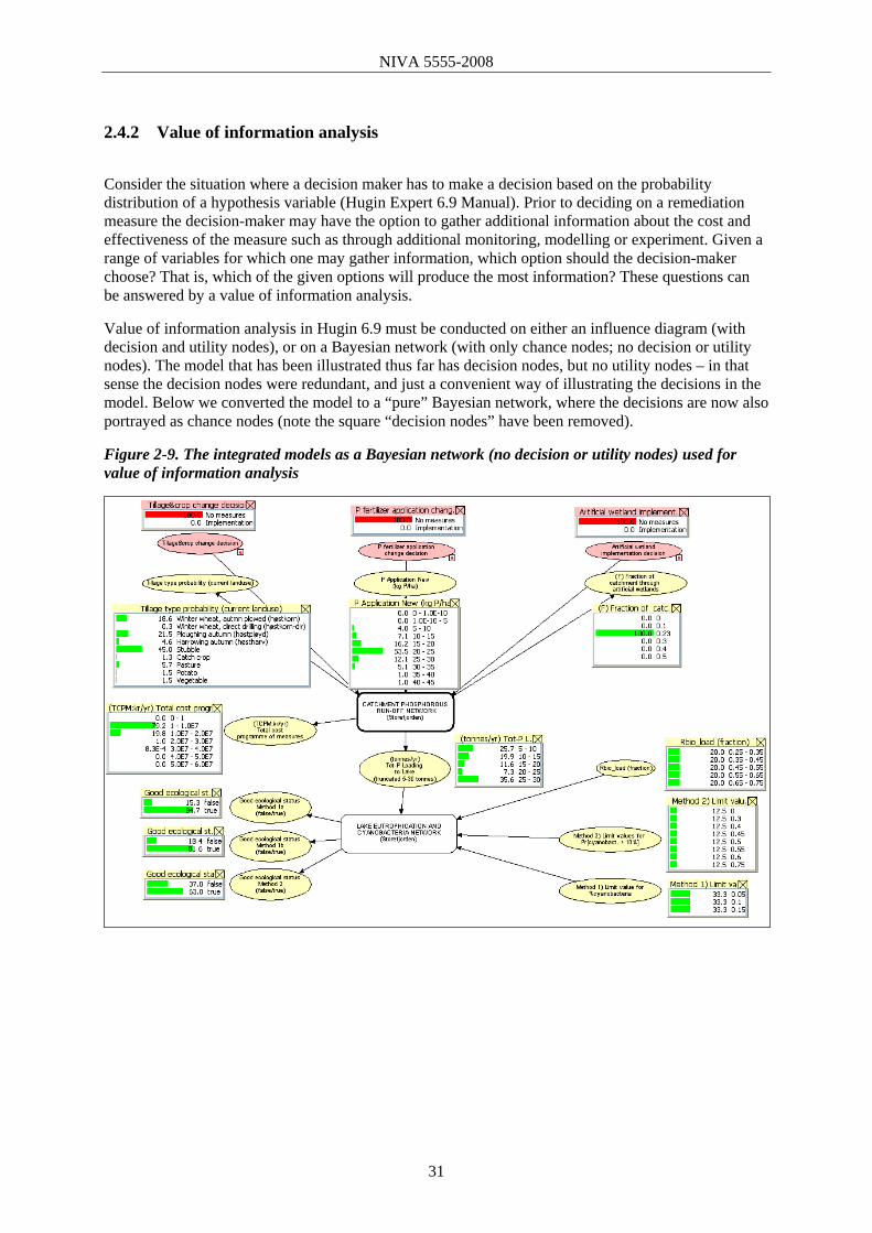
Value of information analysis in Hugin 6.9 must be conducted on either an influence diagram (with decision and utility nodes), or on a Bayesian network (with only chance nodes; no decision or utility nodes). The model that has been illustrated thus far has decision nodes, but no utility nodes – in that sense the decision nodes were redundant, and just a convenient way of illustrating the decisions in the model. Below we converted the model to a “pure” Bayesian network, where the decisions are now also portrayed as chance nodes (note the square “decision nodes” have been removed).

Figure 2-9. The integrated models as a Bayesian network (no decision or utility nodes) used for value of information analysis

31

NIVA 5555-2008

Figure 2-10. Analysis of the value of information of all variables relative to “good ecological status (Method 2)”

Figure 2-10 shows a value of information analysis for the whole integrated model (all variables are evaluated for their contribution to information in “good ecological status (Method 2)”. Unsurprisingly, the definition of the limit value in method 2 is the most important, followed by Tot-P loading to Lake and the fraction of biologically available P (Rbio_load). Amongst the nodes related to remediation measures in the catchment, additional information about tillage type probability would contribute most to knowledge about ecological status in the lake. Figure 2-11. Analysis of the value of information of remediation measure variables in relation to “Total P loading to Lake ”

Figure 2-11 shows a ranking of what variables are of most value observing in the catchment related to remediation measures. Not surprisingly, direct measurement of total agricultural loading (in tributary rivers and streams) gives most information about Total P loading to Lake. Measurement of Total or

32

NIVA 5555-2008

particulate P at the plot level (kg P/ha) is a second best monitoring strategy. As a third best, “erosion SS/ha” followed by “dissolved P”. Observation of soil P concentrations and soil P leaching then follow on the ranking of variables to be observed. 2.4.3 Evidence sensitivity analysis using Hugin In this section we illustrate evidence sensitivity analysis, or so-called“what-if” analysis in Hugin Expert version 6.9. To illustrate what-if analysis, we show the sensitivity of probability of “good ecological status” to different levels of Tot-P loading to Lake Storefjorden, and to the fraction of bioavailable P (Rbio). Figure 2-12, right panel, shows the sensitivity of “good ecological status (method 2)” to different levels of Tot-P loading to Lake Storefjorden in tonnes P per year. As Tot-P loading increases the probability of good status being “true” drops from approximately 90% to 40%. Figure 2-12. What-if analysis – showing sensitivity of “good ecological status (method 2)” to different levels of Tot-P loading to Lake Storefjorden (tonnes/yr).

33

NIVA 5555-2008

Figure 2-13 shows the probability of good ecological status (using method 2) being true/false under different assumptions about the fraction of bioavailable P (Rbio). Assuming Rbio is 0.25-0.35 probability of good status is approximately 80%. If the bioavailable fraction is 0.65-0.75 the probability of good status is approximately 60%. Figure 2-13. What-if analysis – showing sensitivity of “good ecological status (method 2)” to different fractions of bioavailable P.

34

NIVA 5555-2008

2.4.4 Other examples of policy sensitivity analysis The EU project EXIOPOL is evaluating linkages between macro-economic models and catchment level modelling of pollution loading changes, water quality and the economic value of water quality improvements. Macro-economic “computable general equilibrium” (CGE) and “input-output” (I/O) models predict changes in economic activity at the level of a sector and for a whole region, for a whole year at a time. In this section we use the Bayesian network for Lake Storefjorden to explore how scenarios of a % change in agricultural activity could be evaluated. A percentage increase in agricultural activity could be realised in at least three different ways, or a combination of them, which may be evaluated using our model:

1) An increase in spending on pollution mitigation measures. Our model assumes a specific composition of measures which could be employed to evaluate the impacts of changes in the node “total costs of programme of measures”.

2) An increase in the extent of cropping. Given assumptions about the current distribution of

tillage practices we can assume an increase in “agricultural area” at the expense of “non-agricultural area”.

3) An increase in the intensity of land use. Assuming that increased agricultural land-use

intensity is reflected in increased use of fertiliser we can increase “P-application new” relative to “P application current “.

The network for Lake Storefjorden illustrates the extent of assumptions that must be made in order to compute economic damages from water pollution increases associated with increases in agricultural activity. In general, we can say that changes in agricultural economic activity predicted by macro-economic CGE and I/O models will be in the order of tens of percentage points at the most over time periods of several years. Uncertainty and natural variation reflected in the network means that such changes have a relatively marginal impact on expected lake ecological status. Year to year variation in rainfall, erosion and P-loading to lakes such as Storefjorden can be expected to exceed % annual changes in agricultural activity predicted by macro-economic models. In addition to natural variation, the network also expresses uncertainty in our understanding of causal relationships. In order to compute marginal costs of environmental impacts of the agricultural sector on water uses the Bayesian network model would have to be reduced to a deterministic model by setting variables at specific values instead of using probability distributions. These issues are illustrated in the “what-if” analyses below.

35

NIVA 5555-2008

1) An increase in spending on pollution mitigation measures: Figure 2-14 shows that there is a non-linear relationship between spending and tillage practices. This is caused by the fact that different remediation measures, including tillage practices, have different costs. Without any further assumptions about what tillage or other measures are implemented as a result of an increase in economic activity in the agricultural sector, the model uses the cost level to infer which measures are implemented. At different cost levels different combinations of tillage practice are inferred, resulting in non-linear impacts on erosion and finally on ecological status in the lake. Figure 2-14. Sensitivity of “good ecological status” to changes in costs of tillage measures

36

NIVA 5555-2008

2) An increase in the extent of cropping. Figure 2-15 illustrates the sensitivity of ecological status to increases in agricultural loading to Lake Storefjorden. An increase in agricultural loading would be a direct consequence of increasing the area of cropped agricultural land. The model is sensitive to these changes (which are large, implying increases of up to several hundred percent in agricultural area). In practice, land use change is highly restricted in the catchment due to land use regulations and would be restricted to changes of a few percent over a number of years. Figure 2-15. Sensitivity of “good ecological status” to changes in agricultural loading to lake

37

NIVA 5555-2008

3) An increase in land use intensity. Figure 2-16 shows that ecological status is only sensitive to changes in fertiliser application intensity over large changes of up to several hundred percent (rounding hides some of the sensitivity in the figure).

Figure 2-16. Sensitivity of “good ecological status” to changes in new P fertiliser application levels

38

NIVA 5555-2008

3. Lake eutrophication models

3.1

3.1.1

3.1.2

MyLake eutrophication model

Model description The one-dimensional lake model code MyLake (v.1.2) was used to simulate relationships between phosphorus (P) load from the catchment and lake water quality in Lake Vansjø-Storefjorden. MyLake (Multi-year Lake simulation model; Saloranta and Andersen (2004; 2007)) is a process-based model code for simulation of daily vertical distribution of lake water temperature and thus density stratification, evolution of seasonal lake ice and snow cover, sediment-water interactions, and phosphorus-phytoplankton dynamics. A special feature in the MyLake model code development has been the aim to make it well-suited for Monte Carlo simulation (see, e.g., Cullen and Frey, 1999), and thus for application of many comprehensive sensitivity and uncertainty analysis techniques, as well as for simulation of a large number of lakes or over long periods (decades). We have attempted to reach this aim by the use of a professional modelling platform (MATLAB), by making the automated manipulation of the model parameters easy, and by obtaining a relatively short model execution time. Moreover, the basic idea behind the MyLake model code development has been to include only the most significant physical, chemical and biological processes in a well-balanced and robust way. Consequently, MyLake has a relatively simple and transparent model code structure and it is easy to set up for an application. The inclusion of lake ice and snow cover submodel makes MyLake also suitable for simulation of lakes in colder climates. Required data for setting up a MyLake model application are 1) time series of meteorological variables and inflow properties, 2) lake morphometry and initial profiles, and 3) model parameter values.

Model setup and results The MyLake model application and parameterisation in Vansjø-Storefjorden follows closely that described in Saloranta and Andersen (2007). However, in this study the time series of total P (TotP) and suspended solids (SS) concentrations in the water inflow to the lake from a nearby Skuterud monitoring field were used instead of Kure station (Bechmann, pers. comm.). The modelling period was from May 2001 to December 2004, but the (half) year 2001 was considered as a “spin-up” period and thus the results from this period were omitted in later analysis. The model results presented here represent the period 2002-2004. The calibrated model application by Saloranta and Andersen (2007) resulted in 1990-1999 mean June-September TotP and chlorophyll concentrations of 17.4 and 6.5 mg m-3, respectively, in the 0-4 m surface layer. Observations (Stålnacke et al., 2005) show similar concentrations of 17.6 and 6.9 mg m-

3. The simulated mean yearly P load in 1990-1999 was 17.7 tonnes/year with a mean potentially bioavailable P fraction Rbio (defined as the ratio of total reactive P and TotP) of 0.36 on the whole year basis and 0.49 if only June-September was considered. For comparison, Lyche Solheim et al. (2001) estimated a yearly TotP load to Vansjø-Storefjorden of 17.6 tonnes/year and Rbio~0.5 (for summer season) based on data from 1997-1999. Our aim was to construct conditional probability tables (CPTs), i.e. probabilities of different discrete value ranges of water quality variables, conditioned on different discrete value ranges of total yearly P load to the lake and the Rbio in this P load. Our main water quality variables of interest were the 2002-2004 June-September means of TotP and chlorophyll concentration, as well as probability of the fraction of cyanobacteria of total algae biomass exceeding 10 %. The cyanobacteria calculations were based on empirical models (J. Moe & T. Andersen, pers. comm.) using daily water temperature and concentrations of TotP and chlorophyll as predictor variables (see Figure 3-1).

39

NIVA 5555-2008

In order to provide simulation data for calculation of these CPTs the model was run 1300 times (total model execution time ~18 hours) in a Monte Carlo simulation where the inflow concentration time series of TotP and SS (Skuterud data) were scaled with factors CTotP and CSS in order to obtain yearly TotP loads in the range 5-30 tonnes/year and Rbio in this load in the range 0.25-0.75. These scaling factors were in the Monte Carlo simulation sampled randomly from uniform distributions between 0.3-1.9 for CTotP and 0.7-4.2 for CSS on each model run (note that TotP time series is scaled by CTotP while SS time series is scaled by the product CTotP * CSS). When the scaled load was 17.7 tonnes/year with Rbio of 0.36 in this load (corresponding to the calibrated model application by Saloranta and Andersen (2006, submitted ms.) discussed above), then the simulated 2002-2004 mean June-September TotP and chlorophyll concentrations were 17.4 and 6.5 mg m-3, respectively, i.e. equal to those in the calibrated model application by Saloranta and Andersen (2007) discussed above. Currently, the only parameter uncertainties that are taken into account in model simulations (Figure 3-2) are the uncertainties for the three parameters defining the empirical relation between TotP (or chlorophyll), temperature and Pr(>10 % cyanobacteria). Values for these three parameters are sampled on each Monte Carlo simulation round (1300 model runs in total) randomly from normal distributions defined by their standard error estimates, taking also into account the estimated correlations between these parameters in the random sampling. Figure 3-2 shows the simulated 2002-2004 June-September means of TotP, chlorophyll, and Pr(>10 % cyanobacteria) in Lake Vansjø-Storefjorden as function of different total P loads and Rbio in this load. Figure 3-1. Probability of having more than 10 % cyanobacteria in the total algae biomass as function of water temperature and TotP (left panel) or chlorophyll (right panel)

Note: (J. Moe & T. Andersen, pers. comm.). The relation is based on data (1326 samples) from whole Norway. Mean values of the three parameters in the relation are used in the figure.

40

NIVA 5555-2008

Figure 3-2. Simulated 2002-2004 June-September means of TotP, chlorophyll, and Pr(>10 % cyanobacteria) as function of different TotP loads and Rbio in this load, based on the 1300 model runs executed in the Monte Carlo analysis.

Note: Whether TotP or chlorophyll is used with temperature in calculating the Pr(>10 % cyanobacteria) is denoted by “~TP” and “~Chl” in the y-axis label, respectively. 3.1.3 Model sensitivity analysis The sensitivity of the MyLake model application in Vansjø-Storefjorden was analysed by Saloranta and Andersen (2007) using the Extended Fourier Amplitude Sensitivity Test (Extended FAST) global sensitivity analysis method (Saltelli et al. 1999; 2000). In the Extended FAST method values for the model parameters that are included in the analysis are sampled in a wave-like form, so that the amplitude of the particular wave is equal to the parameter’s predefined variation range (e.g., minimum-maximum). The frequencies of the waves are chosen to be incommensurate in such a way that none of the waves can be constructed as a linear combination of the other waves using integer coefficients up to a specific value. Each parameter is thus “labelled” with its own frequency, and the sampling covers well the whole multidimensional parameter space. The model is then run numerous times choosing at each run a new set of parameter values from the wave-like parameter samples, and the model output is monitored. Finally, individual relative contributions of the different parameters on the model output variance can be identified from the periodogram based on the discrete Fourier transformation of the model output. The Extended FAST method reveals both the parameter’s main effect on the model output and the sum of the effects due to its higher-order interactions with other parameters. The sensitivity indices shown in Figure 3-2 reflect both the parameters’ role in the model code and our knowledge of their possible value ranges (Table 3-1). Table 3-1 lists the min-max ranges that were defined for the 13 model parameters that were included in the sensitivity analysis. The model output, for which parameters’ sensitivity was monitored, were

41

NIVA 5555-2008

June-September 2000 mean values of TotP, dissolved reactive phosphorus, chlorophyll and SS in the 0-4 m surface layer. The model was run from May 1999 to September 2000. Sampling rate in Extended FAST was the Nyquist frequency taking into account four harmonics of the basic frequency, and the selected total number of model runs was ~10000. Vertical resolution (Δz) was set to 1 m.

Figure 3-3 shows the sensitivities of the four output variables for the different model parameters. Of all the 13 studied parameters the phytoplankton sedimentation speed wChl and the scaling of TotP concentration in the river inflow (TPIN scaling) were the two most influential parameters for TotP, and similarly, the specific mineralisation rate m(20) and the light saturation level of photosynthesis I’ for dissolved reactive P. For chlorophyll the two most influential parameters were wChl and I’, and for SS, the particle sedimentation speed wSIS and the resuspension rate Ures. In addition, none of the investigated output variables was very sensitive to the model grid size Δz, which indicates that the numerical solution algorithms are working stably in the model code. Figure 3-3. Sensitivity indices, i.e., part of the total variance in model output explained by the 13 parameters analysed by the Extended Fourier Amplitude Sensitivity Test (Extended FAST) sensitivity analysis method.

Note:Studied model output variables are the June-September 1999 mean values of TotP, dissolved reactive P (PD), chlorophyll (PChl), and suspended inorganic particulate matter (SIS) in the 0-4 m surface layer of in Lake Vansjø-Storefjorden, Norway. ”Main effect” denotes the part of total variance explained by the particular parameter alone and “Interactions” similarly the part explained by all parameter interactions where the particular parameter is included. Parameter symbols and their variation ranges used in the sensitivity analysis are explained in Table 3-1.

42

NIVA 5555-2008

Table 3-1. Nominal values of model parameters and minimum-maximum ranges of those included in the sensitivity analysis. parameter value min max remark Δz [m] 1 0.5 2 vertical grid size ak [-] 0.0164 - - turbulent diffusion scaling, open water

period ak [-] 0.000898 - - turbulent diffusion scaling, ice covered

period N2

min [s-2] 7.0×10-5 - - minimum possible stability frequency (N2)

Wstr [-] 0.74 - - wind sheltering parameter I’ [mol m-2 s-1] 3×10-5 10-5 10-4 light saturation level for phytoplankton βC [m2 mg-1] 0.015 0.005 0.045 phytoplankton shading parameter TPIN scaling [-] 0.59 0.4 0.8 scaling of total P conc. in river inflow SISIN scaling [-] 0.89 0.65 1.1 scaling of SS conc. in river inflow ε0 [m-1] 1 0.8 1.3 water PAR attenuation coefficient

(chlorophyll excluded) Ures_epi [m d-1, dry sediment]

3.3×10-7 7.3×10-8 1.8×10-6 resuspension rate for epilimnion

Ures_hypo [m d-1, dry sediment]

3.3×10-8 - - resuspension rate for hypolimnion

Hsed [m] 0.03 - - depth of active sediment layer Psat [mg m-3 ] 2500 - - sediment-water P partitioning isotherm

parameter Fmax [mg kg-3 ] 8000 5000 10000 sediment-water P partitioning isotherm

parameter Fstable [mg kg-3 ] 655 - - sediment-water P partitioning isotherm

parameter wSIS [m d-1] 0.3 0.1 1 sedimentation speed for SS wChl [m d-1] 0.15 0.05 0.5 sedimentation speed for chlorophyll m(20) [d-1] 0.2 0.1 0.3 specific phytoplankton mineralisation

rate at 20° C μ’(20) [d-1] 1.5 1.0 1.5 max. attainable phytoplankton growth

rate at 20° C ksed(20) [d-1] 2.0×10-4 - - sedimented chlorophyll mineralization

rate P’ [mg m3] 0.2 0.2 2 P half-saturation parameter for

phytoplankton

3.2

3.2.1

Cyanobacteria model

Model description The sub-network in Figure 3-4 links the TotP load (predicted by MyLake) to the proportion of cyanobacteria and to subsequent assessment of lake status. The sub-network was modelled by three alternative methods (Method 1a, Method 1b, and Method 2). In addition, both TotP and Chl-a were used as alternative predictor variables. Here the model based on TotP will be described. The main difference between the methods was the construction of the conditional probability tables (CPTs) that linked predicted the proportion of cyanobacteria (nodes 4, 5 and 11). For methods 1a and 1b, the CPT was calculated from the empirical relationship between TotP and %cyanobacteria (Figure 3-5A). For

43

NIVA 5555-2008

method 2, a statistical model (logistic regression) was used to estimate the relationship between TotP and the probability of %cyanobacteria > 10. The estimated statistical relationship was then used to predict the probability of %cyanobacteria > 10 from TotP load. Figure 3-4. Bayesian network model for eutrophication in Lake Storfjorden: sub-network representing the links from phosphorus load to cyanobacterial blooms. The figure displays the model based on total phosphorus (TP) concentrations predicted by the model MyLake (a corresponding network based on predicted Chlorophyll a (Chl-a) concentrations is also analysed). The network contains three parallel methods with different CPTs (conditional probability tables) for the link from the predictor variable (TP or Chl a) to the response variable (risk of cyanobacterial bloom): Method 1a: CPTs based on empirical relationship; Chl-a node has regular intervals. Method 1b: CPTs based on empirical relationship; Chl-a node has irregular intervals determined by regression tree analysis. Method 2b: CPTs based on statistical relationship (logistic regression). 3.2.2 Data and discretisation The data used for parametrising the sub-network from TotP load to %cyanobacteria are mainly from the regional eutrophication survey in 1988 (describe in Lyche-Solheim et al. 2004), additional samples are from 1989-2001. We have selected samples from months 5-9, from all counties of Norway. Only samples with information on TotP, Chl-a, %cyanobacteria and temperature were used, in total 1326 of out of 2521 samples. Methods 1a and 1b differed by the discretisation of the of the TotP node (alternatively, the Chl-a node). For Method 1a, the borders between the intervals were not set at specific values, but with regular distances except for the last interval (0, 5, 10, 15, 20, 25, 30, 35, 40, Inf). For Method 1b, the borders were selected by a regression method called Classification and Regression Trees (CART). We have used the package “rpart” (Recursive Partitioning and Regression Trees; Therneau & Atkinson 2006) in the statistical software R (R Development Core Team 2006). This regression method is not dependent on distributions, and is thus more robust than ordinary regression methods. The regression tree helped optimising TotP intervals in such a way that variation in %cyanobacteria values was low within the intervals and high among the intervals. The resulting interval borders were 0, 11, 16, 23, 29, 46, 56, Inf. For the Chl-a node, the original regular intervals were 0, 3, 6, 9, 12, 15, 18, 21, Inf, and the intervals determined by CART were 0, 6, 15, 28, 49, 100, Inf.

44

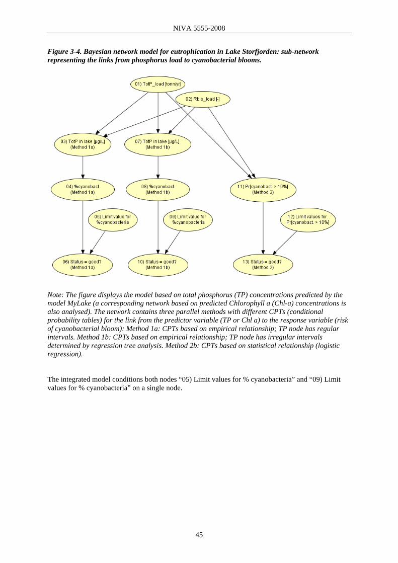
NIVA 5555-2008

Figure 3-4. Bayesian network model for eutrophication in Lake Storfjorden: sub-network representing the links from phosphorus load to cyanobacterial blooms.

Note: The figure displays the model based on total phosphorus (TP) concentrations predicted by the model MyLake (a corresponding network based on predicted Chlorophyll a (Chl-a) concentrations is also analysed). The network contains three parallel methods with different CPTs (conditional probability tables) for the link from the predictor variable (TP or Chl a) to the response variable (risk of cyanobacterial bloom): Method 1a: CPTs based on empirical relationship; TP node has regular intervals. Method 1b: CPTs based on empirical relationship; TP node has irregular intervals determined by regression tree analysis. Method 2b: CPTs based on statistical relationship (logistic regression). The integrated model conditions both nodes “05) Limit values for % cyanobacteria” and “09) Limit values for % cyanobacteria” on a single node.

45

NIVA 5555-2008

3.2.3 Results and sensitivity analysis Entropy of predictor node (Table 5-2) is lower for Method 1b (where node intervals are determined by a regression tree analysis). This implies that the information (on the distribution of the predictor node values) is better preserved in method 1b. The lower number of intervals for the predictor node in Method 1b compared to 1a contributes to the reduction in entropy. Table 3-2. Sensitivity analysis. Lower entropy value normally indicates that the predictor node is more informative. Scenario Entropy of

predictor node (Tot P or Chl-a)

Sensitivity of response node (%cyanobacteria or P[cyano>10%])

to variation in Tot P load Method 1a Method 1b Method 1a Method 1b Method 2

Pred

icto

r va

riab

le

Tot

P Best 0.84 0.71

Default 1.92 1.58 2.85 % 2.93 % 41.2% Worst 1.58 0.93

Chl

-a Best 1.0 0.53

Default 1.84 0.98 3.98 % 4.21 % 31.7 % Worst 1.78 0.69

For the response node (cyanobacteria), the entropy value is not so useful as a measure of information preservation. The reason is that the distribution of cyanobacteria is not unimodal: there is a very high probability of low values, a low probability of intermediate values, and a somewhat higher probability of very high values. Here, Method 1b better predicts of the probabilities of high %cyanobacteria, but this results in higher entropy (because the information is more scattered on both low and high values of %cyanobacteria). In this case, the higher entropy should be interpreted as a higher probability of detecting the extreme events of cyanobacterial blooms. The sensitivity of the response nodes to variation in TotP load (Table 3-2) is higher for Method 1b than for Method 1a. This results shows that Method 1b has succeeded in in setting intervals that better represents changes in the TotP - Chl-a relationship than the regular intervals in Method 1a do. For Method 2, however, the sensitivity is around 10 times higher. This shows that the signal (effect of TotP variation on Chla concentration) is much stronger in this version. 3.2.4 Assessment of ecological status: alternative approaches Figure 3-6 summarises the assessments for the three methods, using either TotP or Chl-a as a predictor variable. For all three methods, the model predicts a reduced probability of status = good, as could be expected. When TotP is used as predictor, Method 1b gives a slightliy stricter assessment (lower probability of status = good) than Method 1a, while the opposite is the case when Chl-a is used as predictor. Method 2, however, gives a much stricter assessment than Methods 1 and 2. Here TotP as predictor gives a considerably stricter assessment than Chl-a.

46

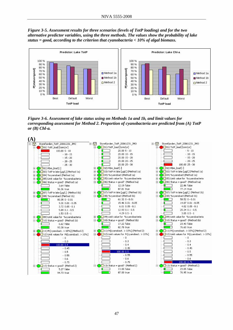
NIVA 5555-2008

Figure 3-5. Assessment results for three scenarios (levels of TotP loading) and for the two alternative predictor variables, using the three methods. The values show the probability of lake status = good, according to the criterion that cyanobacteria < 10% of algal biomass.

Predictor: Lake TotP

0 %10 %20 %30 %40 %50 %60 %70 %80 %90 %

100 %

Best Default Worst

TotP load

P[st

atus

=goo

d]

Method 1a

Method 1b

Method 2

Predictor: Lake Chl-a

0 %10 %20 %30 %40 %50 %60 %70 %80 %90 %

100 %

Best Default Worst

TotP load

P[st

atus

=goo

d]

Method 1a

Method 1b

Method 2

Figure 3-6. Assessment of lake status using on Methods 1a and 1b, and limit values for corresponding assessment for Method 2. Proportion of cyanobacteria are predicted from (A) TotP or (B) Chl-a. (A)

47

NIVA 5555-2008

(B)

48

NIVA 5555-2008

49

4. Nutrient loading model

The nutrient loading model illustrated in Figure 4-1 is based on our present knowledge, measured values and expert opinion on processes causing P losses from agricultural areas. The underlying understanding of processes has been described by Haygarth and Jarvis (1999). They have built a conceptual model where they split P loss processes into different forms and pathways. The total P transfer comprises a soluble mode of transfer, particulate mode of transfer and transfers when fertilizer/dung or manure is removed from the land surface coincident with hydrological factors. The hydrological pathways consist of 1) saturated and preferential flow transferring P through the soil to the tile drains, ground water or directly to the stream water and 2) overland flow causing erosion, intersurface and incidental transfer of P. These processes are represented in the model structure. The components are set up in a similar way as in the P index (Sharpley et al., 2003; Bechmann et al., 2007). The network describing nutrient loading is driven by decisions (red square nodes) regarding changes in tillage practices (upper left hand), P application changes (upper right hand) and artificial wetland implementation (middle). The effects of tillage practices on particle P loading and of P application on dissolved P leaching from soil are modified by the extent of catchment run-off treated by artificial wetlands. The decisions regarding tillage, fertilisation and artificial wetlands lead to changes in costs which are calculated in sub-networks (shown in white). In section 5 the sub-networks for calculating costs of measures are discussed. Below we discuss the different P pathways illustrated in Figure 4-1 in detail.

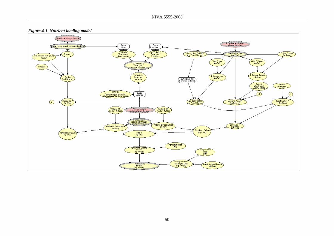
NIVA 5555-2008

Figure 4-1. Nutrient loading model

50

4.1 Tillage and crop changes In this section we look in detail at the part of the nutrient loading network dedicated to calculating particle loading (Figure 4-2).

Figure 4-2. Section of nutrient loading model illustrating particle loading process

Note: upper left hand side of Figure 4-1 “Catchment phosphorus run-off network (Storefjorden”).

Erosion is one of the most important processes causing P losses in Norway. Besides the natural factors causing risk of erosion, e.g. slope, soil texture and precipitation, the soil management is important for the total risk of erosion. To describe the influence of soil management on erosion risk, Lundekvam (2002) has developed factors that quantify the effect in relation to a standard soil management. The standard soil management is defined by a combination of spring cereals and autumn ploughing and are developed for the region Romerike. Soil erosion risk maps (Norwegian Institute for Forest and Landscape) are available for most agricultural soil in Norway at this standard soil management. However, in the present model we derived the KLS-factor from the soil mapping and developed a precipitation factor for the actual area. The soil management factor (C-factor) describing the effect of crops grown and the soil tillage is presented in Figure 4-3. The effect of soil management on erosion may differ for different areas. For example for flat areas there may be nearly no effect of reduced soil tillage on erosion risk. In this approach a simplification of the C-factor is chosen, meaning that the C-factor does not differ for the different erosion risk of the areas. However, the probability distribution describes the variability of the C-factor. In the model structure it is possible to include the variability in C-factor caused by difference in slope and soil (KLS), if more specific data are available. The estimated erosion in the catchment of Lake Storefjorden is calculated as the sum for all areas of the multiplied K*LS factor, precipitation factor and the soil management factor. Erosion and soil P status is combined to give the final particulate P loading.

51

NIVA 5555-2008

Figure 4-3. Probability estimates for the soil management factor (C-factor) for erosion risk.

0-0,

025

0,02

5-0,

05

0,05

-0,1

0,1-

0,15

0,15

-0,2

0,2-

0,25

0,25

-0,3

0,3-

0,4

0,4-

0,5

0,5-

0,6

0,6-

0,7

0,7-

0,8

0,8-

0,9

0,9-

1

1-1,

1

1,1-

1,2

1,2-

1,5

WW-AP

WW-DD

APLAH

STCC

PASTPOT

VEG

0

0,1

0,2

0,3

0,4

0,5

0,6

WW-APWW-DDAPLAHSTCCPASTPOTVEG

Note: WW-AP=winter wheat, autumn ploughing; WW-DD=winter wheat, direct drilling; APL=autumn ploughing; AH=autumn harrowing; ST=stubble; CC=catch crop; PAST=pasture;POT=potato; VEG=vegetables. The KLS factor does have an appropriate mass in the upper interval (21.8%). However, in earlier version of the model the Erosion factor had a very large mass in the upper interval, since 50,8% of the area is in the erosion risk class from 0-500. In the latest version of the network the discretisation of the erosion factor was changed to represent more classes in the lower range from 0-500. The classes are now 0-100, 100-200, 200-300, 300-400, 400-500, 500-600, 600-700, 700-1000, 1000-2000, 2000-8000, 8000-14000. The data for risk of soil erosion are derived from the National soil type maps (Norwegian Institute for Forest and Landscape). The uncertainty in the erosion risk-data itself is not included in our approach, however the distribution of data show the spatial distribution of soil erosion risk in the lake catchments. The same method is used for the soil management and crop distribution. These data are based on national statistics (SSB) for the actual areas and describe the spatial variation in soil management for the case study areas.

52

NIVA 5555-2008

4.2 Soil P content and P leaching Figure 4-4. Section of nutrient loading model for calculating soil P content and P leaching

Note: upper right hand side of Figure 4-1“Catchment phosphorus run-off network (Storefjorden”). Phosphorus application practices and resulting soil P content and P leaching are calculated in the part of the network illustrated in Figure 4-4. The “P application change decision” conditions “P application new” which contains a set of rules for reduced P application dependant on the soil P status. The P application is unchanged from the current (in 2005) where the soil P-AL is below 5. Between P-AL 5 and 10, the P application can be max P yield minus 0.5 kg/ha. Between 10 and 15, the P application can be max P yield minus 5 kg/ha. Above P-AL 15, the P application is zero. Current soil P In Morsa the highest values measured are in the 40s. Values up to 100 has, however, been measured in other intensive agricultural areas. The data in Current soil P are in fact actual empirical distribution for current soil P. Current soil P and New soil P should have approx. the same discretization. We have suggested 0-5, 5-10, 10-15, 15-20, 20-25, 25-30, 30-35, 35-100.

53

NIVA 5555-2008

We have shown the distribution and the uncertainty in current soil P by giving the factor a probability mass in the upper and lower intervals. The lowest interval is based on measured P content in forest soils and the highest interval is based on P content in livestock/vegetable areas. The mass in each class is based on spatial distribution in the Morsa catchment. Particulate P The soil P content determines the transfer of particulate P in eroded particles. The soil P status (P-AL) at present is used to estimate the P content of eroded particles at present. An increase in soil P status (P-AL) increases the soil P content, though this is not a linear relationship. The new soil P content (in 2015) is calculated by: max (Current Soil P + tot_soilP_change_1_1_b * P_Surplus_New, 0), which means that the soil P status in 2015 is influenced by current soil P, the soil P change during these years and the P balance (P application minus P in yields) in crop production. The “P_Surplus_New” is a nutrient balance between the new P application based on the soil P status and P yield. Leaching of dissolved P The leaching of P from soil is calculated by P leaching= 0.02*runoff*P-AL*10. The total annual rainfall in mm is used as a scaling factor for the P transfer. We have used a linear relationship between P-AL and P leaching, though some results suggest that the P leaching may increase exponentially by increased soil P status. Dissolved P from applied P (incidental transfer) The risk of P transfer from surface applied P is generally low. It depends on the risk of getting high rainfall in a period after P application. Runoff after P application was estimated based on data from Skuterud catchment 1994-2006 in the spring period 25. April to 15. May (20 days), which gave a yearly mean of 15.8 mm (Rspring) and std. dev. of 7.7 mm. The loss of applied P = (e1 * Rspring * PAN, 0). The e1 is estimated to 100 µg P/L for cereal areas in spring and represents a parameter for dissolved P in runoff after P application. PAN is P application new represents the P application scenario. Total dissolved P The amount of dissolved P transfer is the sum of Leaching of dissolved P and dissolved P from applied P (incidental transfer). Total Particulate P transfer The total transfer of particulate P (PP) is calculated from the estimated erosion risk and the P content of these soil particles (SS) as follows: PP = SS * a* PAL. P-AL constitutes 10% of the total P and there is an enrichment factor of 1.3, which gives a mean value of a=1.3e-4. The distribution of "a" is based on expert evaluations. 4.3 Artificial wetlands Figure 4-5 illustrates the section of the nutrient loading model dedicated to calculating the effect of artificial wetlands on dissolved P and particulate P loading. At the catchment scale the effect of wetlands are calculated from the fraction of the catchment draining through a wetland. The effect of wetlands on P transfer in agricultural dominated catchments differs for different forms of P and hence

54

NIVA 5555-2008

the effect is calculated for dissolved P transfer and for particulate P transfer separately. The effect of wetlands on the particulate P loading is hence calculated from the share of the catchment draining through a wetland (F) and the effect of wetland on the particulate P as follows: PP(in) = F * PPloss. And PP (out) = (1 - WPP) * PP (in), where WPP is the retention factor. A similar approach is used for DP. Figure 4-5. Section of nutrient loading model illustrating the effect of artificial wetlands on dissolved P and particulate P loading

Note: lower middle part of Figure 4-1“Catchment phosphorus run-off network (Storefjorden”). 4.4 Total catchment loading The total P loading per ha of the agricultural area in the catchment is calculated as the sum of dissolved P and particulate P out of the wetland. To obtain the total loading information on the total agricultural area is included. The estimated contributions from forested and other areas within the catchment are based on standard values of P loading for these areas: Non-Agricultural Loading to Lake (NALL) = Non-agricultural area * Non-agricultural loading. The total Loading to Lake is then the sum of Agricultural Loading to Lake and Non-Agricultural Loading to Lake. Total loading to Lake = (ALL + NALL) / 1000 in kg/yr. Empirical data (kg P/ha) to compare the distribution of particulate P loss is difficult. We have measured data for the Hobølelva, but these data show only temporal variation. The variation in the network is not temporal but spatial. We have no spatial data to compare the results from our network. We have a set of data from lysimeter studies all over the country that could possibly be used for comparison, but these data were not at hand and they may not all be relevant for the conditions in Morsa. This is a weak point of our network, but at present we don't see a possibility to validate our results.

55

NIVA 5555-2008

5. Nutrient abatement costs

5.1 Tillage and crop changes Figure 5-1 illustrates the sub-network for calculating the costs of tillage and cropping changes. Figure 5-1. Sub-network for costs of tillage and crop changes

Expected annual costs of different tillage types were based on Framstad and Stalleland (1997). Costs are given in 2005 Norwegian kroner and are financial costs to the farmer of each type of tillage. An assumption of a +/-10% variation of the expected values were based loosely on a study of variation in returns to the 13 worst and 13 best wheat farms out of a sample 100 in South Eastern Norway (Haug, 2007). (i.e. using a discrete distribution we assume that 13% of farms have tillage costs 10% below the mean, and 13% of farms have tillage costs 10% above the mean.) Total costs of tillage (TCT) are calculated as the product of tillage costs per unit of area and agricultural area. Total costs of subsidies for reduced ploughing measures are also calculated in the model, based on state subsidy rates allocated at county level8. Cost of subsidies are not used in the calculation of total costs, but provided as a reference for decision-makers. 5.2

P-Application changes Figure 5-2 illustrates the sub-network used to calculate the costs of P application. Total cost of phosphorus fertiliser is the product of P application per unit of area, agricultural area and a so-called shadow price for phosphorus. A shadow price is an implicit price that takes into account the variation of the price of the compound fertiliser as a function of the relative amounts of its constituents. Calculation of a shadow price is necessary given that the cost of phosphorus as a raw material in fertiliser may misrepresent the actual cost of phosphorus in the actual fertiliser applied by farmers. A linear programming (LP) model (Rørstad 2006) was used on 8 different fertiliser compunds of N-P-K based on fertiliser prices for 1987-2005. LP modelling was carried out by Per Kristian Rørstad (University of Life Sciences).

8 Veiledende satser. Miljøtilskudd forurensning, Fylkesmannen i Østfold.

56

NIVA 5555-2008

Figure 5-2. Sub-network for costs of P application

Figure 5-3 shows the different fertiliser compounds used to calculate a shadow price for P (a pure P fertiliser was also included). The vertical axis indicates the (shadow) price of P. Figure 5-4 shows the average shadow price across compound fertilisers as compared to the price of a pure phosphate fertiliser and raw phosphate as input in other fertilisers. The average shadow price is the lower of the three and can be regarded as a conservative estimate of cost savings on changing to a fertiliser with lower P content. The shadow price of P shows large variation which is reflected in the probability distribution used in the network. Reasons for this is the small number of fertiliser compounds used in the LP model, variation in the price of raw materials (oil/gas), producers pricing of their products which cannot be attributed to the cost of the input factors, and the fertilisers have other characteristics that are not captured by the N-K-P relationship (pers. com. P.K. Rørstad). Figure 5-3. Fertiliser prices for different fertiliser compunds of N-P-K, 1987-2006, used in linear programming model of shadow price of P.

Note : « full fertiliser « N-P-K composition. Vertical axis : shadow price P. Source: personal communication Per Kristian Rørstad, IØR-UMB

57

NIVA 5555-2008

Figure 5-4. Shadow price of P compared to prices for raw P (“råfosfat”) and a simple P-fertiliser

Source: personal communication Per Kristian Rørstad, IØR-UMB.”Enkelt super”= pure P fertiliser;”råfosfat= price of raw phosphate. Vertical axis is the shadow price of P. 5.3 Artificial wetlands Figure 5-5 illustrates the sub-network for calculating the costs of constructing and maintaining artificial wetlands in the catchment. Figure 5-5. Sub-network for costs of artificial wetlands

The abatement measure is determined by the fraction of catchment assumed to be draining through artificial wetlands. Also, the recommended proportion of a wetland area (WA) to the total catchment area determines total wetland area. This is an expert recommendation determined by hydraulic

58

NIVA 5555-2008

loading. Lyche Solheim et al. (2001) suggest that WA=0,1% for Morsa whereas Framstad og Stalleland(1997) have used 0,1%-0,25% in Jæren in Western Norway. A particular issue arisesexpressing the geographical extent of measures in the Bayesian network. Discretisation of catchment area as as an interval distribution would lead to information loss relative to our knowledge of the fraction of the catchment over which the wetlands will drain. A numbered distribution is thereforeused - the network therefore only performs for predetermined scenarios of the fraction of catchmenunder wetlands.

when

t

he distribution for “average fixed costs” (AFC) of wetlands is based on actual costs and catchment

Total fixed costs wetlands”(FC) is the expected investment cost of wetlands. This network assumes

ixed Cost= 71,066*catchment area + 70695

Variable costs” (VC) of wetland maintenance were set at kr 588/daa yr (Stalleland og Framstad,

n annualisation factor for fixed costs =0,12 (10 years, 4% discount rate) is used to convert costs to

Total costs wetlands” per year is the sum of fixed and variable annual costs (TACW=AF * FC +

Tareas drained for 39 wetlands that have been constructed in the Morsa catchment (pers.com. Helga Gunnarsdottir, Morsa Project). “that wetland investment costs are proportional to catchment area drained, and are independent of the number of wetlands (as if a single wetland was scaled to fit total run-off for catchment). Four of the most expensive wetland projects removed from the distribution (about 11% of sample). We use the cost/area data directly as an empirical distribution. The following parametric approach was not used,but illustrates a significant relationship between fixed costs and catchment area draining to artificial wetlands: FR2 = 0,5185 “1997:4). Aannual figures which can be compared to annual tillage and fertiliser costs. “TWA * VC).

59

NIVA 5555-2008

6. Stakeholder defined cause-effect networks for abatement measures

Bayesian networks are well suited to exploring causes and effects in a qualitative way before proceding to quantification of relationships between them using conditional probabilities (see e.g. Bromley et al. 2005). Using the “graphical user interface” (GUI) of Bayesian network software and group participation methodologies, the problem structure can be explored and information gaps be identified taking advantage of local stakeholder expertise. Stakeholders definition of the problem universe using cause-effect diagrams may also help to uncover “methodological uncertainties”, i.e. factors that have not been included in the quantitative networks for want of data, models or expertise on how to treat them. Two workshops were conducted with stakeholders in the Morsa catchment to define such cause effect diagrams for the three eutrophication abatement measures considered in the EutroBayes project. See the Appendix for a description of the participative methodology used to generate the networks with stakeholders9.

The three abatement measures suggested by researchers for modelling was validated with the participants at the workshop.

• Artificial wetlands

• Reduced tillage • Reduced fertiliser

application Participants at the workshop requested to focus their evaluations on measures in the catchment of Vestre Vansjø, where eutrophication problems are at the worst. The cause-effect networks they generated are of general interest in the rest of the Morsa catchment

draining to the Storefjorden (which is one of two lakes that have been modelled in this report). The

Figure 6-1. The stakeholder evaluation of abatement measures focused on reduced tillage, reduced fertilisation and artificial wetlands

Source: adapted from Fylkesmannen i Østfold. Tilskudd til Regionale Miljøtiltak (2005)

9 Meetings were held in May and September 2006. Stakeholders/local expert participating in the definition of the different networks were: Reduced Fertiliser Application: Gerd Guren (LFR, agricultural), Peder Unum (Våler kommune) Reduced Tillage: Helga Gunnarsdottir (Morsa Project), Kristian Navestad (farmer) Artificial wetlands: Tyre Risnes Høyås (County of Østfold, FMOS), Karsten Butenschøn (Morsa Project), Knut Berg(LFR), Facilitators: David N. Barton (NIVA) and Marianne Bechmann (Bioforsk)

60

NIVA 5555-2008

Storefjorden had been the object of several years of previous monitoring and modelling and was chosen at the beginning of the EutroBayes project as the easiest location in which to conduct a “proof of principle” using Bayesian networks. However, this does point to the fact that our modelling research experiences a time lag relative to managers’ current focus in the catchment. The groups’ cause-effect networks (Figures 6-2, 6-3 and 6-4 below) are qualitatively different compared to the quantitative networks discussed in this report, one is not necessarily more valid than the other. However, a more in depth comparison of the qualitative and quantitative networks would be of interest to the extent that it uncovers:

(i) Implementation uncertainty. Explanations of cost-effectiveness which are not technical or

biophysical - e.g. factors that uncover the extent of implementation among farmers. (ii) Omitted variables. Other technical or biophysical drivers than those defined by

researchers. (iii) Uncertainty perception. Information gaps in the technical and biophysical factors which

researchers on the other hand deem to be of low uncertainty

Local stakeholders/experts recommended that sociological aspects have a greater role in future modelling exercises. The quantitative models in this report assume a 100% implementation rate of the abatement measures that are defined – uncertainty is wholly technical-biophysical. The comments stakeholders made to their own diagrammes reflect the lack of sociological explanations of uncertainty of the cost and effect of measures. Reduced fertiliser application Figure 6-2 shows the local stakeholder definition of factors affecting the cost-effectiveness of reduced fertiliser application. The most signficant variables and information gaps are identified (the network is evaluated for row crops such as potato). Main information gaps identified by stakeholders regarding cost-effectiveness of measures (reduced fertilisation)

• political priority setting of the implementation of fertilisation standards • research on fertilisation standards • availability of information and guidance to farmers on fertilisation practices • incremental costs of reduced fertiliser application and the effect of financial incentives on farmers

Stakeholder comments to reduced fertilisation measures (Figure 6-2) Due to limited research on fertilisation norms, agricultural extension services have limited advice on how low they can recommend farmers to go in phosphate content of fertilisers when the soil P-Al levels are high, without impacting crop yields. Many possible explanations of the cost-effectiveness of reduced fertilisation exist because so little research is available to farmers regarding crop yield functions of phosphate application. Factors include fertiliser amount, fertiliser composition (P-K-N), number of applications, cropping practices, soil P levels, soil pH, temperature etc. There are a number of ways for authorities to regulate reduced P application, but also ways for farmers to compensate for regulations. Currently, fertilisation practices largely do not take into account existing soil P levels. Fertilisation practices are influenced by market demand for crop quality (e.g. potatoes). Fertiliser vendors provide advice alongside agricultural extension services with little normative guidelines from authorities.

61

NIVA 5555-2008

Figure 6-2. Reduced fertiliser application

In summary, uncertainty concerning the cost-effectiveness of reduced fertilisation as a measure is perceived to be both political, regulatory and due to lacking research on recommended fertilisation norms. Political and regulatory uncertainty is wholly absent from the quantitative networks evaluated in this report. Fertilisation norms are based on researchers “best guesses” in our quantitative network without access to crop yield functions. Artificial wetlands Figure 6-3 illustrates stakeholders understanding of determinants of cost-effectiveness of artificial wetlands. Main information gaps identified by stakeholders regarding cost-effectiveness of measures (artificial wetlands)

• Access to peer experiences with artificial wetlands • Financial incentives • Legal basis for mandatory implementation • Fertilisation practices in catchments draining to wetlands • Direct losses of animal manure

62

NIVA 5555-2008

Figure 6-3. Artificial wetlands

Stakeholder comments to artificial wetland measures (Figure 6-3) A number of sociological and financial factors affect how many wetlands are constructed. Once wetlands are built their effectiveness is determined almost entirely by natural and technical factors. The use of financial incentives depends on the authorities – currently the Agricultural Agreement (Landbruksavtalen) is used to promote environmental measures. This means that the amount allocated to financial incentives competes with other agricultural interests. This means that the availability of financial incentives from year to year is highly uncertain. Because there is a lot of physical variation across sub-catchments where artificial wetlands are implemented, local erosion risk and fertilisation practices will determine how effective wetlands are. The correlation of high erosion risk, high soil-P areas with sub-catchments draining to artificial wetlands is not captured in the quantitative networks considered in this report. In other words our networks do not consider the coordinated targeting of measures, but assumes that they have an equal probability of implementation across the study area. This weakness is uncovered by the stakeholder cause-effect diagram.

63

NIVA 5555-2008

Reduced tillage Figure 6-4 illustrates stakeholders’ evaluation of factors affecting the cost-effectiveness of reduced tillage measures. Figure 6-4. Reduced tillage

Main information gaps identified by stakeholders regarding cost-effectiveness of measures (reduced tillage)

• Climate • Effects of channelisation • Interplay between information, capacity-building and existing local knowledge (which is

strong for established tillage practices) Stakeholder comments to reduced tillage measures (Figure 6-4) Sanctions and subsidies have greater effectiveness on farms with small economic returns. This is not considered in the cause effect diagram. The degree to which implementation of changed tillage practices depends on farm(er) characteristics is not considered in the quantitative networks in this report.

64

NIVA 5555-2008

7. Model transferability between sites

One aim of the EutroBayes project was to evaluate the transferability of Bayesian network models between case study sites. To what extent is site specific data (the unconditional nodes in the network) at Lake Steinsfjorden comparable to Lake Storefjorden? Would it results in very different cost-effectiveness results? For this purpose the initial model was developed for the Lake Storefjorden case and then the question asked of data acquisition in the Lake Steinsfjorden case (Figure 7-1). This chapter therefore describes the two case study sites only in terms of the site specific characteristics that condition the effectiveness of nutrient abatement measures (the unconditional nodes of the network). Figure 7-1. Location of Steinsfjorden and Storefjorden lakes evaluated for model transfer

Source: NVE Atlas The review of available data on abatement measures reveals gaps in catchment specific data for key variables (e.g. distribution of soil P levels) which mean that experts would generally use the same distributions in both catchments. Cost-effectiveness conclusions could be expected to be broadly similar, and we have not set up a separate model for Steinsfjorden.

65

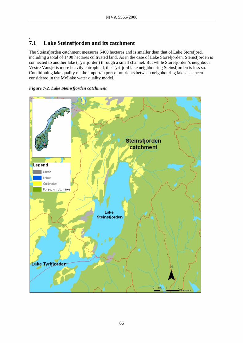
NIVA 5555-2008

. 7.1 Lake Steinsfjorden and its catchment The Steinsfjorden catchment measures 6400 hectares and is smaller than that of Lake Storefjord, including a total of 1400 hectares cultivated land. As in the case of Lake Storefjorden, Steinsfjorden is connected to another lake (Tyrifjorden) through a small channel. But while Storefjorden’s neighbour Vestre Vansjø is more heavily eutrophied, the Tyrifjord lake neighbouring Steinsfjorden is less so. Conditioning lake quality on the import/export of nutrients between neighbouring lakes has been considered in the MyLake water quality model. Figure 7-2. Lake Steinsfjorden catchment

66

NIVA 5555-2008

7.2 Erosion risk Erosion risk Lake Storefjorden Lake Storefjorden Erosion risk estimates consist of a topographic factor (LS), a soil erodibility factor (K) , a weather factor (R) (Figure 7-3) and a soil management factor (C). The soil management (production and soil tillage) is available on farm scale from Statistics Norway (SSB) (Figure 3-4). Yield is based on the farmers deliveries to Unikorn. The LS and K factors are derived from soil type maps produced by the Norwegian Institute for Forest and Landscape. The R factor is a combined effect of precipitation and snow melt, and is based on calibrated value for the Skuterud catchment in The Norwegian Monitoring Programme for Soil management and Water quality. The figures show the spatial distribution of the factors for the catchment of Lake Storefjorden. (http://www.skogoglandskap.no/kart/temakart_erosjon

Erosion risk estimates consist of a topographic factor (LS), a soil erodibility factor (K) , a weather factor (R) (Figure 7-3) and a soil management factor (C). The soil management (production and soil tillage) is available on farm scale from Statistics Norway (SSB) (Figure 3-4). Yield is based on the farmers deliveries to Unikorn. The LS and K factors are derived from soil type maps produced by the Norwegian Institute for Forest and Landscape. The R factor is a combined effect of precipitation and snow melt, and is based on calibrated value for the Skuterud catchment in The Norwegian Monitoring Programme for Soil management and Water quality. The figures show the spatial distribution of the factors for the catchment of Lake Storefjorden. (http://www.skogoglandskap.no/kart/temakart_erosjon). Figure 7-3. The spatial distribution of the soil (K) times the topographic (LS) factor

Lake Storefjorden catchment Steinsfjorden catchment Steinsfjorden The sources for data on erosion risk and land use are the same as for Storefjorden. There is however no JOVA-catchment in the neighbourhood of Steinsfjorden, so the distribution of the weather factor (R) is based on the distribution for Storefjorden and scaled relatively by the yearly normal precipitation. From a mean value of 283 for R in Storefjord, this gives a mean value for Steinsfjorden of 200. The distribution is also made a bit wider due to more variation in topography in the Steinsfjorden catchment than in the Storefjorden's. Figure 7-4. Distribution of the weather factor (R) in the catchment of Storefjord

as for Storefjorden but scaled by yearly normal precipitation

Lake Storefjorden catchment Steinsfjorden catchment

67

NIVA 5555-2008

7.3 Crop distribution and management Storefjorden The actual soil management before implementing measures consisted of 45% of the area in stubble during winter, 21% autumn ploughing, 19% winter wheat with ploughing. Agricultural measures can be modelled flexibly to study any land use scenario of interest in the Bayesian network. In this report a single scenario was analysed in which there was no autumn ploughing, as well as changing the area with autumn tilled winter wheat to direct drilled winter wheat. As a consequence, the distribution of the area in stubble became 67% and the direct drilled winter wheat 19% of the agricultural area. Figure 7-5. The area distribution of the crops and soil management in the catchment before and after implementation of measures.

Storefjorden Steinsfjorden

Steinsfjorden While the distribution of the area in stubble and the direct drilled winter wheat under implementation of reduced ploughing measures is the same, the current situation in Steinsfjorden is somewhat different from Storefjorden. The proportion of spring cereals with autumn ploughing was much larger, while the proportion under stubble was much lower in Steinsfjorden than Storefjorden. This may be because the Storefjorden catchment has for some years been the focus of additional subsidies for reduced ploughing. Consequently, the effect of the same policy proposal would be larger in Steinsfjorden than Storefjorden. The effect on water quality in Steinsfjorden however depends on the relative importance of reduced ploughing measures relative to other measures. 7.4 Soil P status The soil P status (P-AL) at present is derived from the National Soil Databank (Bioforsk) for the actual areas. In the case of Storefjorden more updated information was available and the last year of data was used (2005). In the case of Steinsfjorden the last 15 years of data were used to generate a distribution. The distributions of soil-P are nonetheless almost identical. A large weakness of the soil P data sets is that the soil-P values have not been weighted by area before being used in the Bayesian network. This means that high soil P figures may be over-represented and low soil P figures under-represented relative to area generating run-off. We would expect a lack of area-weighting to exaggerate the variation in soil P, thereby increasing uncertainty in the effect of measures.

68

NIVA 5555-2008

Figure 7-6. Soil P status (P-AL in mg/100g)

Storefjorden Steinsfjorden

7.5 Soil P application Current fertiliser application levels are compared in Figure 7-7. Fertiliser application per hectare exhibits less variation in Storefjorden catchment than the Steinsfjorden catchment, but is broadly similar in terms of average fertilisation per hectare. A large limitation of the P application data available is that it is available only for cereals and meadow. While this covers the majority of cultivated area in both catchments, potato and vegetable production are also known to have much higher fertilisation levels per unit area. The data in our model treats all cultivated area as cereals/meadow, when particular cost-effective reduction in fertiliser application may be found when targeted to vegetables and potatoes. Figure 7-7. Distribution of current P application, based on the 1999 Agricultural Census.

Storefjorden Steinsfjorden

69

NIVA 5555-2008

7.6 Crop yields The crop yields of cereals are available due to subsidies dependent on the amount of cereals the farmers delivers to the mills (Unikorn). On other crops, this information is scarce or not available. The yield of phosphorus is based on standard figures of P-content in the different cereals. The distribution however is an educated guess.

due to subsidies dependent on the amount of cereals the farmers delivers to the mills (Unikorn). On other crops, this information is scarce or not available. The yield of phosphorus is based on standard figures of P-content in the different cereals. The distribution however is an educated guess. Figure 7-8. Distribution of crop P yield Figure 7-8. Distribution of crop P yield

Storefjorden Steinsfjorden

According to the statistics of cereal deliveries to the mills, crop yields in the Steinsfjorden catchment are about 500-1000 kg/ha higher than in the Storefjorden catchment. The distribution of P yields is based on the distribution in the Storefjorden catchment, but shifted upwards to reflect this difference. As both distributions are based on expert “best guesses” it is not possible to evaluate the transferability of this data. 7.7 Conclusions regarding transferability across catchments The main limitations to transfering the conclusions on effectiveness and cost-effectiveness of measures from the Storefjorden to the Steinsfjorden catchment are:

• Current soil-P levels determine the recommended changes in P application under “reduced fertilisation” measures evaluated in the model. However, soil-P data is not weighted by the area each value represents. The probability distribution in the model therefore simply represents the number of observations in the dataset, rather than the probability of finding a given soil-P level when choosing a random hectare of cultivated land in the catchment. The only way to rectify this would be to evaluate whether land-use features with GIS coverage could be correlated with P-Al measurements, and then used to area-weight the P-Al observations.

• P application was not differentiated by crop type, with data available only for cereals and meadow. While area cultivated for vegetables and potatoes in Storefjorden catchment is small, reductions in fertiliser applications there may be highly cost-effective. Currently, there is no area under vegetables in the Steinsfjorden catchment so the use of cereals and meadows data may be more acceptable.

• Large difference in crop yield were observed between Steinsfjorden and Storefjorden catchments, while P application levels were broadly similar. This means that a greater proportion of applied P is exported from the Steinsfjorden catchment in the form of crop yield. Reduced fertiliser application measures in Steinsfjorden are therefore expected to have lower cost-effectiveness.

70

NIVA 5555-2008

In general, the status quo land-use and productivity is different between catchments. A given policy such as reduced fertilisation or prohibiting all autumn ploughing in favour of winter stubble in wheat will therefore have different effects on run-off, and different cost-effectiveness. However, the sensitivity analysis in the section 3 shows that within-site variation and modelling uncertainty may be as great as between site differences, thereby overshadowing errors due to transferring conclusions between sites.

71

NIVA 5555-2008

8. Discussion and future research questions

Stakeholder and researcher validation The researchers involved in the nutrient loading, abatement costs and lake quality sub-networks set out to create a model or network which would be as simple as possible, i.e. with as few nodes as possible. The lake model had only 13 nodes in total, but could have been reduced to only 7 as 6 of the nodes were due to alternative methodological approaches that were tested. The nutrient loading network had a total of 48 nodes, while the abatement cost sub-networks had a total of 20 nodes. In the prior case, the modelling complexity was incorporated in the underlying MyLake and cyanobacteria analytical models, while in the latter two cases the networks were based on empirical models and expert judgement. This illustrates Bayesian networks flexibility in adjusting to and integrating the information available and discipline specific knowledge. It also illustrates a trade-off between providing enough detail for validation of network assumption by independent researchers, while keeping the network focused on issues that are of interest to stakeholders and decision-makers. An approach to deal with this trade-off would be to use sub-networks to a greater extent to “hide” technical relationships that were unimportant for providing an overview of the model for stakeholders, while making modelling assumptions directly available to researchers in the network (rather than through references to underlying models). It is also revealing to contrast the issues that stakeholders find relevant when they construct causal chains of nutrient abatement, with what the EutroBayes researchers found relevant and were able to model. The comparison was undertaken for the part of the network relating to nutrient loading. Across all the measures, the main conclusion from the stakeholder constructed models was the lacking information on farmers’ degree of implementation of measures, conditional on legal and financial incentives that would be put in place. Due to the composisiton/priorities of the research team, there was no focus in the EutroBayes project on modelling of farmer behaviour. All uncertainty relating to implementation of measures was technical and biophysical. Future extensions to this work would focus on building a sub-network to evaluate the probability of farmer adoption of the nutrient abatement measures. Integrated model The integrated model represent a proof of principle approach, and uses available models, data and expert opinion. It is not possible to validate the conclusions of the integrated model in the sense of testing against data from monitoring or against an experiment. The only sub-network which was calibrated and validated in the statistical sense was the lake eutrophication model. Therefore, the credibility of the model depends crucially on the credibility of the experts who provided their “best guesses” on probability distributions and relationships. Furthermore, the integrated model must be transparent enough for decision-makers to quickly be able to see probability distributions and relationships between the variables. Finally, water quality and ecological status under the “current situation” must represent decision-makers understanding and the direction and magnitude of effects of abatement measures must be intuitively correct. The integrated network for Lake Storefjorden and its catchment fulfils these criteria on some, but not all counts. In general, verification of expected water quality for the baseline / historical situation can be validated, while the variance cannot. The catchment phosphorus run-off network generates expected tot-P loading to the lake in accordance with monitoring data. However, the variance of Tot-P loading is greater than the historical data suggest.

72

NIVA 5555-2008

One technical explanation is that the probability distributions conditioning nutrient loading due to measures are also active under the “no implementation” scenario. A solution is to (instantiate) nutrient loading into the lake model at the level actually observed, so that variability in erosion, fertiliser application and wetland implementation don’t inflate uncertainty. Ecological status depends crucially on the definition of threshold between moderate and good status, and the confidence levels decision-makers require to characterise something as good status. These thresholds are currently being evaluated in Norway in the context of the EU Framework Directive. When decided the nodes representing this uncertainty can be removed from the model, or “set” at the given value. The integrated model provides perhaps some counter-intuitive results in the magnitude of changes caused by the measures. For any given definition of threshold levels of good ecological status, the three abatement measures collectively implemented only result in approximately a 10 %-units increase in the probability of good ecological status. The magnitude of the measures is large: around 2500 additional hectares of winter wheat as “stubble” instead of e.g. autumn plowing, more than 700 additional hectares of agricultural land draining to artificial wetlands; and an approximate halving of mean P application/hectare. We have not evaluated the benefit of a 10 %-units increase in the probability of good ecological status and compared them to abatement costs. A previous study of a different programme of measures, not including fertiliser reduction, found costs to be larger than benefits to willingness to pay for measures for recreation (Barton, 2008). Physical lake and cyanobacteria sub-network The simple Monte Carlo simulation based uncertainty analysis approach used for the lake network will provide a straightforward and easy way to propagate some specific parameter uncertainties into the nutrient abatement scenario results. However, a Markov chain Monte Carlo based technique might in the future be preferred for combined model calibration and uncertainty analysis, as this technique is well-suited for tracing and quantifying both parameter unidentifiabilities (i.e., different parameter value combinations may produce the same model result), correlations and uncertainties (see e.g. Gamerman, 1997; Larssen et al., 2006). In this way also the model prediction uncertainties, due to uncertainties in model parameter values, will be integrated in the CPTs simulated by the model. This type of model parameter uncertainties is also called technical uncertainties. However, there may also be significant uncertainties of another type which are not accounted for in a usual uncertainty analysis, e.g uncertainties in how well the scientific knowledge behind the algorithms in the model code describes reality (methodological uncertainties) or uncertainties due to presently unknown processes of e.g. nutrient behaviour in a catchment or a lake (epistemological uncertainties). Below are listed some important processes that are not included in the model, but which may potentially affect the dynamics of the lake system. These processes represent thus a potential source of methodological uncertainties.

• As phytoplankton is in the model represented by a single state variable (chlorophyll) the model cannot itself simulate shifts in the composition of the phytoplankton community. However, values of the phytoplankton related parameters can in principle be changed during a simulation, so reflecting possible changes in the composition of the phytoplankton community.

73

NIVA 5555-2008

• Population dynamics of the phytoplankton-predating species (or the food web in general) are not simulated in the model. All phytoplankton loss processes (predation, respiration, lysis, parasitism, etc.) are aggregated to a single first-order remineralisation process. However, values of this loss rate parameter can be changed during a simulation, so reflecting possible changes in the predator populations.

• As nitrogen dynamics are not simulated in the MyLake model, the model cannot simulate

properly cases where the phytoplankton growth in the lake would turn to be nitrogen limited. The most urgent simulation model development needs are therefore:

• the inclusion of MCMC techniques to calibrate the model applications and analyse and take into account model parameter uncertainties in the resulting simulated CPTs;

• development of MyLake model code to better represent phytoplankton dynamics and

differences in the composition of phytoplankton (e.g. between the two subbasins of Lake Vansjø), e.g. by including two different algae groups in the model.

Cyanobacteria modelling questions A number of modelling questions were raised in the cyanobacteria component of the lake sub-network. How can model sensitivity be assessed, when entropy is not an appropriate measure? This is relevant when a distribution can be expected to be bimodal, such as proportion of cyanobacteria (we can expect either very low or very high values, but not intermediate). A more sensitive model will be able to predict also the very high values (more bimodal distribution), and will thereby have higher entropy. In this case higher entropy should not be interpreted as lower information10. What methods can be used to for obtaining an optimal discretisation, i.e. that gives most "sensitive" network with the fewest number of intervals? How should the sensitivity be weighted against the number of intervals? Could this be done by some sort of cross-validation, as in statistical model selection? Regression tree analysis was attempted and indicated a more optimal approach to discretisation (although computationally more demanding). Value-of-information analysis: The value of obtaining new information that may affect a decision, and thus costs and benefits, can be assessed within a Bayesian network (influence diagram). This kind of value-of-information analysis is most relevant for situations where completely new information can be obtained. In the case of lake monitoring, however, a more relevant situation will be to increase the number of samples of phytoplankton and/or chemistry. A higher number of samples will not give new information, but it can reduce the uncertainty (give higher precision and accuracy) of the measured values. How can this reduced uncertainty be evaluated? Can this be taken into account in some sort of value-of-information analysis? Nutrient loading and costs of abatement measures sub-networks The nutrient loading model is built on knowledge on known processes and pathways. However, the model has not been validated on independent datasets. The model only represents a first simplified 10 New versions of Hugin 6.9 now have “parameter sensitivity analysis” features which can be used in simple networks (disabled for OOBNs and Influence Diagrams).

74

NIVA 5555-2008

approach to a complicated model structure. Especially the lack of area-based probability weighing of different processes may not be realistic. The data sources for defining probability distributions for abatement costs of tillage, fertiliser application and construction of artificial wetlands are of varying quality. Although a specific study on costs of tillage practices was available for the Morsa / Lake Storefjorden catchment, it is now more than 10 years old. Furthermore, it contains only point estimates of costs with no information which may be used to determine the uncertainty or probability distributions. Variations in financial returns to different farms in South Eastern Norway are probably only weakly related to variations in tillage practice costs. The uncertainty about tillage costs is therefore probably underestimated. Costs of changing inputs of phosphate are calculated indirectly through the shadow price of phosphate in fertiliser compounds. While this shadow or implicit price represents variation due to variation in fertiliser prices and composition, it does not reflect any incremental costs farmers may have in changing their fertilisation practices. Such costs are assumed to be zero, and this may be reasonable for reductions in fertiliser use. Given the use of fertiliser compounds may not have exactly the fraction of phosphate suggested by the ideal P application rules specified in the network, farmers may not implement the P application suggestions exactly as specified. This leads to uncertainty in both P application and costs which is not captured in the model (methodological uncertainty) Cost data for artificial wetlands is the most accurate of the three sub-networks. We use the empirical distribution of historical wetland construction costs from the Morsa catchment which drains to Lake Storefjorden. To the extent that variation in historical costs reflects the variation in conditions under which wetlands in new sub-catchments may be built, this is as accurate a description of cost uncertainty as we can expect to get. However, only a single estimate was available on the maintenance costs of artificial wetland. Variation in operating costs is expected to be lower than for construction costs, but we don’t know by how much.

75

NIVA 5555-2008

9. Conclusion

For any given definition of threshold levels of good ecological status, the three abatement measures collectively implemented result in approximately a 10 %-units increase in the probability of good ecological status. The magnitude of the measures is large: around 2500 additional hectares of winter wheat as “stubble” instead of e.g. autumn ploughing, more than 700 additional hectares of agricultural land draining to artificial wetlands; and an approximate halving of mean P application/hectare. We have not evaluated the benefit of a 10 %-units increase in the probability of good ecological status and compared them to abatement costs. A previous study of a different programme of measures, not including fertiliser reduction, found costs to be larger than benefits to willingness to pay for measures for recreation (Barton et al. 2008). Our networks do not consider the coordinated targeting of measures, but assumes that they have an equal probability of implementation across the study area. This weakness is uncovered by the stakeholder cause-effect diagrams discussed in chapter 6. . What is the ecological status of Lake Storefjorden today as it might be described in a River Basin characterisation report under the Water Framework Directive? Basing ecological status only on the cyanobacteria criteria (for demonstration purposes), Storefjorden is in “good status” with probabilities ranging from 63% to 84,7% depending on the classification method chosen (Figure 9-1). Figure 9-1. Network illustrating “no measures” or status quo probabilities

76

NIVA 5555-2008

What are the effects of implementing a proposed package of measures including reduced tillage (stubble instead of autumn ploughing) , reduced fertiliser application and doubling of area of artificial wetlands? The effect of these measures is to increase the probability of good status from 63% to 73.5% (Figure 9-2). Figure 9-2. Network illustrating a scenario “with measures”

Reduced fertiliser application is the most effective in reducing P-loading and increasing the probability of good status, as well as being a cost-saving measure. A savings of kr. 1000 in P input costs11 results in a reduction of 2.28 kg of P loading to Storefjorden and is a “win-win” measure. Reduced ploughing measures is more cost-effective than artificial wetland construction relative to tot-P loading (Table 9-1). Cost effectiveness is shown to be much lower for reduced tillage and artificial wetland than in the most recent impact assessment from the catchment using a deterministic (no uncertainty) approach. 11 Using a computed shadow price for phosphate (see chapter 5)

77

NIVA 5555-2008

Table 9-1 Cost-effectiveness of measures Measure Low-high estimate effect/cost

(reduction kg Tot-P /thousand kroner) Lyche Solheim et al 2001 (p.68)

Expected effect/cost (reduction kg Tot-P /thousand kroner) This study

Cost-effectiveness ranking This study

Reduced fertiliser use

n.a. -2.28 1

Reduced tillage 4.00 - 11.11 1.14 2

Artificial wetlands alone

0.88 - 2.04 0.18 3

Note: reduced fertiliser use is a cost-saving measure for reducing Tot-P loading (positive effect divided by negative costs). The EutroBayes project has used Bayesian networks to bring together three different aspects of assessing the impacts of nutrient abatement measures; abatement costs, nutrient loading, and lake water quality. These aspects are brought together to conduct an assessment of the status quo in the Lake Steinsfjorden catchment, describing a baseline scenario which captures natural variation. The method can be used in the context of the assessment of measures under the Water Framework Directive. The EU Water Framework Directive requires that river basin authorities carry out a “river basin characterisation report” describing the current ecological status of water bodies, the risk of not reaching “good ecological status” and describing a baseline situation against which the effectiveness of measures is to be evaluated12. The guidance does not specify how to deal with natural variation, as well as uncertainty due to lacking data. Ecological status is not a static status quo situation, but rather depends on natural climate induced variation. In cases where uncertainty in the current ecological status is important, Bayesian networks offer an approach to documenting available knowledge on causes and effects this in a way that can be used in later assessments of measures. A programme of measures to achieve good ecological status or potential is called for under the Norwegian regulation on implementing the WFD – in Norway about 20% of river basin are so called “1st phase areas” and will need development of a programme of measures by 2009. Norwegian authorities have developed a Guidance Document for the assessment of environmental measures under the WFD13. The guidance document recommends that local authorities document the effects of measures at source (end-of-pipe, end-of-field) and use a qualitative 3 level scale to describe the scope and magnitude of effects of measures (p.21). This recommendation has been made based on the recognition that knowledge and data on dose-response relationships is poor at the municipal level which is charged with conducting the assessments. This leaves ample room for expert judgement, but the guidance offers little in the way of specific requirements for documenting this judgement. 12 “Metodikk for Karakterisering av Vannforekomster i Norge”. Versjon 1, 13.08.07 http://www.vannportalen.no/hoved.aspx?m=45147 13 ”Veileder i Arbeidet med Miljøtiltak”, Direktoratsgruppen, Versjon 1. 12.09.07 http://www.vannportalen.no/hoved.aspx?m=45149 )

78

NIVA 5555-2008

Despite the use of a simple effect scale in evaluating the cost-effectiveness of measures the Guidance goes on to recommend that a number of considerations be documented in judging effect (p 22):

Seasonal variation Delays in impact Distance from the site of abatement measures to the water body Documentation of effects of measures using monitoring data Other site specific conditions

As the example in this report show, Bayesian networks can be used to document available quantitative data on these issues alongside documentation of expert judgement of impacts. Using available quantative models and expert judgement we have shown how the Bayesian network can be used to conduct cost-effectiveness analysis, taking explicit account of uncertainty. However, the greatest relevance of the Bayesian network methodology to assessments under the WFD is in the context of evaluating “derogations” from the objective of good ecological status. The guidance document states that an “ample margin of error” should be considered and that measures should be considered in conjunction with one another (pp. 34). Assessments of derrogations requires that one answer the question of whether abatement costs are “disproportional” (to the benefits of achieving good ecological status). Assessing disproportionality and knowing what “margin of errors” one is dealing with requires a quantitative approach which Bayesian networks is well suited to handle. Furthermore, the conditional nature of causal chains means that one can assess the joint effect of different combinations of measures. The Guidance document also calls for the assessment of the cost-effectiveness measures using a “stepwise backwards” approach where the least cost-effective measures are removed one by one simulatenously assessing the achievement of good ecological status. In the senstivity analysis in this report we demonstrate how Bayesian networks can be used to reason in a recursive way (“inductively”), answering the question, what level and combination of measures do we need in order to achieve “good ecological status” with a certain probability level. The EutroBayes project would seem to have demonstrated that Bayesian networks are a tool that can be used for risk analysis in integrated assessments of measures under the Water Framework Directive. What will be needed to bring Bayesian networks from the research arena to use in practical policy assessment? We can use the experiences from the nutrient abatement example in this report to answer the question. The gaps are related to (i) limitation in communication of risk in policy assessment, (ii) methodological uncertainty, and (iii)software:

(i) Main communication gaps:

• Costs and effects are described in terms of probability distributions which in popular terms is often translated into “uncertainty”. A greater focus on what level of certainty policy recommendations were made under would be a more pedagogical approach to communicating results from the Bayesian network. In this study, the probability of good ecological status increased by 10 %-units in Lake Storefjorden as the result of a programme of measures.

• “Bayesian networks” is a technical terms that does not translate well in practical policy

analysis circles. A focus on “quantitative risk / impact analysis” would be more familiar to policy makers in Norway.

79

NIVA 5555-2008

(ii) Main methodological gaps:

• A Bayesian network describes probabilities of environmental conditions (e.g. erosion risk, soil P levels) across a defined catchment. GIS data is required to quantify the proportion (probability) of different conditions taking place. This was lacking for soil P and P yield in crops, making it difficult to correctly estimate probabilities of reduced fertilisation measures.

• The model assumes 100% and immediate implementation of measures among farmers, and

that the farmer only has technical implementation costs (i.e. no additional time costs regarding paper work). This overstates the cost-effectiveness of measures, as well as underestimating variability across farms in the catchment. Future models should focus on the probability of farmer implementation of measures given different types of incentives (financial, legal).

• A simple model of plankton communities was used without population dynamics. Nitrogen

dynamics was not included in the lake model. Not modelling nitrogen limitation and interaction between algae communities, as well as the role of greater climate variability, means that predictions of cyanobacteria levels probably underestimated variability.

• The example in this report focused a single criteria for “good ecological status”. In practice

ecological status will be determined by a number of different “quality elements” (macroinvertebrates, phytoplankton, phytobenthos, macrophytes, macroalgae, angiosperms, fish, chemical water quality) which will complicate a quantitative analysis of the risk of not achieving good status. Bayesian networks would be a useful tool in evaluating the importance of each quality element in the probability of achieving good status.

(iii) Main software/technical limitations: • Bayesian networks assume a given time frame over which variation is evaluated. They are

best suited to evaluating abatement measures whose impacts can be evaluated in a single year (bacteriological, eutrophication, accute spills). Multi-period and feed-back effects are not easily dealt with, making it less suited to evaluate e.g. persistent pollutants.

• Bayesian networks assume a given space over which variation is evaluated. For probabilities

to be correctly and consistently computed data source should have the same spatial scope.

• The way probability distributions are split up into intervals (“discretised”) can affect results. This needs to be tested using sensitivity analysis.

The main alternative to Bayesian networks in cost-effectiveness analysis as currently practiced in impact assessment is the spreadsheet (e.g. Lyche Solheim et al. 2001). All the limitations stated above also apply to spreadsheet models. The three great disadvantages of spreadsheet models in relation to Bayesian network are that they (i) do not consider variability (unless used in conjunction with simulation tools such as @Risk), (ii) do not visualise the problem structure or cause-effect chain, and (iii) they cannot be used for “recursive” or inductive reasoning. We feel that these are three strong reasons to give further consideration to Bayesian networks in quantitative risk and impact assessment under the Water Framework Directive.

80

NIVA 5555-2008

10. References

Barton, D. N., Saloranta, T., Moe, S. J., Eggestad, H. O. & Kuikka, S. 2008: Bayesian belief networks

as a meta-modelling tool in integrated river basin management – Pros and cons in evaluating nutrient abatement decisions under uncertainty in a Norwegian river basin. Ecological Economics 66: 91-104.

Barton, D. N., T. Saloranta, S. J. Moe, H.O.Eggestad, N.Vagstad, A. L. Solheim and J. R. Selvik (2006). Using belief networks in pollution abatement planning. Example from Morsa catchment, South Eastern Norway. NIVA Report SNo.5213-2006, Norwegian Institute for Water Research (NIVA).

Bechmann ME, Stålnacke P, Kværnø SK. 2007. Testing the Norwegian Phosphorus Index at the field scale. Agriculture, Ecosystems and Environment 120: 107-128.

Bromley, J., N. A. Jackson, O.J. Clymer, A.M. Giacomello, F.V. Jensen (2005). The use of Hugin to

develop Bayesian networks as an aid to integrated water resource planning. Environmental Modelling & Software 20: 231-242.

Cullen, A. C. and Frey, H. C., 1999. Probabilistic techniques in exposure assessment. Plenum Press,

New York, NY, 335 pp. Framstad B. and T. Stalleland (1997) Tiltak for å bedre vannkvaliteten i øvre del av Hobøl-Langen

vassdraget. Notat 1997:10 UTKAST. Norsk institutt for landbruksøkonomisk forskning (NILF) Gamerman, D. (1999). Markov Chain Monte Carlo: Stochastic simulation for Bayesian inference;

Chapman & Hall: London, UK. Haug (2007). Økonomien I jordbruket på Østlandet. Utviklingstrekk 2001-2005. Tabellsamling 2001-

2005. Senter for matpolitikk og marked (SeMM). Norsk institutt for landbruksøkonomisk forskning (NILF)

Haygarth, P. and Jarvis, S.C. 1999. Transfer of phosphorus from agricultural soils. Advances in

Agronomy 66: 195-249. Larssen, T., Huseby, R. B., Cosby, B. J., Høst, G., Høgåsen, T. and Aldrin, M. (2006). Forecasting

acidification effects using a Bayesian calibration and uncertainty propagation approach. Environ. Sci. Technol.40: 7841-7847.

Lyche Solheim. A., Vagstad, N., Kraft, P., Turtumøygard, S., Skoglund, S., Løvstad, Ø., Selvik, J.R.,

2001. Tiltaksanalyse for Morsa, Vansjø-Hobol-vassdraget: sluttrapport. NIVA rapport 4377-2001, Norwegian Institute for Water Research, Oslo, Norway, 104 pp. (in Norwegian).

Lundekvam H, ERONOR/USLENO - Empirical erosion models for Norwegian conditions. Report no.

6/2002. ISBN: 82-483-0022-6. pp 40. Kjærulff, U. B. and A. L. Madsen (2005). Probabilistic Networks - An Introduction to Bayesian

Networks and Influence Diagrams, Department of Computer Science, Aalborg University and HUGIN Expert A/S.

81

NIVA 5555-2008

R Development Core Team (2006). R: A language and environment for statistical computing. R Foundation for Statistical Computing, Vienna, Austria. ISBN 3-900051-07-0, URL http://www.R-project.org.

Rørstad, P.K.(2006) Økonomiske vurderinger av gjødslingspraksis I et JOVA-felt. Diskusjonsnotat

DP-01/06. Institutt for økonomi og ressursforvaltning. Universitetet for Miljø- og Biovitenskap. Saloranta, T. M. and Andersen, T. (2004). MyLake v. 1.1: technical documentation & user’s guide.

NIVA report 4838, Norwegian Institute for Water Research. Saloranta, T. M. and Andersen, T. (2007). MyLake – A multi-year lake simulation model suitable for

uncertainty and sensitivity analysis simulations. Ecol. Model. 207: 45-60. Saltelli, A., Tarantola, S., Chan, KP-S., and Scott, E. M. (1999). A quantitative model-independent

method for global sensitivity analysis of model output. Technometrics 41: 39-56. Saltelli, A., Chan, K., and Scott, E. M. (2000). Sensitivity analysis. Wiley; New York. Sharpley, A. N., Weld, J. L., Beegle, D. B., Kleinman, P. J. A., Gburek, W. L., Moore P. A. and

Mullins G. 2003. Development of phosphorus indices for nutrient management planning strategies in the U.S. Journal of Soil and Water Conservation 58: 137-152.

Solheim, A., Andersen, T., Brettum, P., Bækken, T., Bongard, T., Moy, F., Kroglund T., Olsgard, F. ,

Rygg, B. , Oug, E. (2004). BIOKLASS - Klassifisering av økologiske status i norske vannforekomster. Forslag til aktuelle kriterier og foreløpige grenseverdier mellom god og moderat økologisk status for utvalgte elementer og påvirkninger. NIVA report no. OR-4860. 63 pp.

Stalleland T. and Framstad B. (1997) Tiltak for å bedre vannkvaliteten i vassdrag på Jæren. Notat

1997:4. Norsk institutt for landbruksøkonomisk forskning (NILF) Stålnacke, P. G., Lyche Solheim, A. and Bechmann, M., 2005. Utvikling av vannkvaliteten i

Hobølelva og Vansjø: En foreløpig analyse av tidsserier. NIVA rapport 4937, Norwegian Institute for Water Research, Oslo, Norway, 30 pp. (in Norwegian).

Therneau, T. M. and B. Atkinson. R port by Brian Ripley <ripley@stats.ox.ac.uk>. (2006). rpart:

Recursive Partitioning. R package version 3.1-32. S-PLUS 6.x original at http://mayoresearch.mayo.edu/mayo/research/biostat/splusfunctions.cfm

82

NIVA 5555-2008

11. Appendix 1

KORT OPPSUMMERING - TRINN I Å LAGE EN ”PÅVIRKNINGSMODELL” AV TILTAK I JORDBRUKET. Trinn Oppgaver

Kort og generell beskrivelse av tiltaket (redusert jordbearbeiding, redusert gjødsling, fangdammer)

1

Hva er tiltaksmålet? Det kan være flere mål som tiltaket skal oppnå, for eksempel være kostnadseffektivt og ha stor total effekt på fosfor-reduksjoner med mer.

2

Hva er måleenhet skal brukes i rapportering av måloppnåelse? (for eksempel kostnadseffektivitet: kr./kg tot-P)

3

Hvilke faktorer påvirker måloppnåelse? Lage en liste på et A4 ark over de viktigste basert på egen kunnskap, erfaring og ”magefølelse”. Prøv å gruppere dem under kategorier som ”Naturgitte faktorer”, ”Tekniske faktorer”, ”Juridiske og administrative faktorer”, ”Økonomiske faktorer” etc. Skriv så navn på faktorene (maks 2-3 ord) ned på Post-It lapper og klistre dem på tavlene i omtrent en logisk årsak-virkning rekkefølge.

4

Hvordan påvirker faktorene hverandre? Bruk tusjpenn til å trekke piler på tavlen mellom faktorene i årsak-virkning retningen. Flytt på Post-It lapper og piler etter behov for å få en oversiktelig ”påvirkningsmodell” som kan forklares til andre grupper.

5

Hvordan kan du måle påvirkningsfaktorene (målenheter)? Skriv i (parentes) på Post-It lappene hvordan faktorene kan måles hvis man skulle skaffe informasjon om dem i forbindelse med tiltaksgjennomføring (for eksempel målbare enheter (kg løst fosfor), eller kvalitativt (ja/nei), (mye/lite), (høy-medium-lav), (1…6) etc.

6

Fanger ”påvirkningsmodellen” opp de viktigste faktorene og sammenhengene? Hvis ikke legg til faktorer og årsak-virkning piler etter behov.

7

Hvilke av faktorene har størst innflytelse på målsettingen? Se på alle faktorene som ikke er påvirket av noe annet i påvirkningsmodellen (ikke har noen piler inn i seg). På venstre side av hver Post-It og med blå tusjpenn, skriv ned et tall som viser om faktoren har svært stor innflytelse (=1), noe midt imellom(=2-8), eller svært liten innflytelse (=9).

8

9 Hvilke faktorer vet vi minst om? Se på de samme faktorene som i trinnet over. På høyre side av hver Post-It og med rød tusjpenn, skriv ned et tall som viser om faktoren har svært stor usikkerhet (=1), noe midt imellom(=2-8), eller svært liten usikkerhet (=9). Usikkerhet om faktoren kan skyldes (i) manglende forståelse av prosesser, (ii) manglende data om prosesser, (ii) eller naturgitt variasjon (eller en kombinasjon av i-iii).

10 Hvor har vi informasjonsgap? Se på de blå og røde tallene på hver faktor. Hvilke faktorer har stor innflytelse, men har også stor usikkerhet ? Hvilke av faktorene kan vi gjøre noe med på kort sikt, på lang sikt, eller ikke i det hele tatt? Oppsummering og presentasjon av gruppearbeidet 11 Felles diskusjon. Hva har kommet ut av denne øvelsen av nytte for Tiltaksplanen for Vestre Vansjø? For eksempel, oppfølging av informasjonsgap. Kan vi redusere informasjonsgapene (trinn 10) ved å beskrive påvirende faktorer i større detalj? Hvilke overvåknings eller utredningsoppgaver bør inkluderes i tiltaksplanen for å redusere disse informasjonsgapene?

12

83

NIVA 5555-2008

Summary of experiences with the stakeholder method of cause-effect networks The group’s composition dictates which variables/factors are selected in the model. A group composed of many different interests is expected to produce cause-effect networks of greater relevance for integrated modelling. Composing groups of experts within the same domain produces models with greater detail. Comparison of cause-effect networks for the same measures across different groups of experts is useful for uncovering methodological uncertainties in the factors affecting effectiveness of abatement measures. Some particular comments regarding the methodology were:

• Scoring of “importance” and “uncertainty” for the different factors was not clear enough (high versus low score)

• More time should have been spent on evaluating other objectives of the measures than simply cost-effectiveness of reductions in P loading

• Networks are easier to construct “branch-by-branch”, startin with the objective, than first making a complete list of factors and then linking these together. However, the branch-by-branch approach can lead to omission of some causal factors.

84

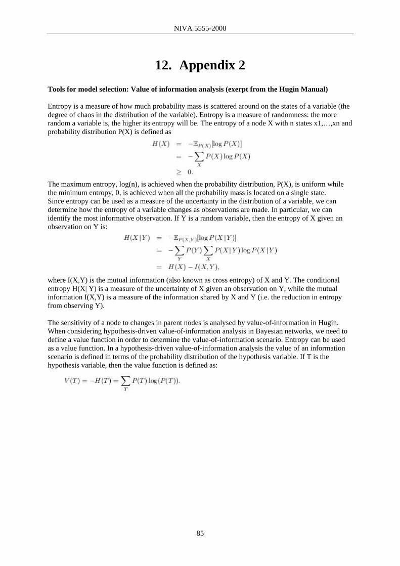
NIVA 5555-2008

85

12. Appendix 2

Tools for model selection: Value of information analysis (exerpt from the Hugin Manual) Entropy is a measure of how much probability mass is scattered around on the states of a variable (the degree of chaos in the distribution of the variable). Entropy is a measure of randomness: the more random a variable is, the higher its entropy will be. The entropy of a node X with n states x1,…,xn and probability distribution P(X) is defined as

The maximum entropy, log(n), is achieved when the probability distribution, P(X), is uniform while the minimum entropy, 0, is achieved when all the probability mass is located on a single state. Since entropy can be used as a measure of the uncertainty in the distribution of a variable, we can determine how the entropy of a variable changes as observations are made. In particular, we can identify the most informative observation. If Y is a random variable, then the entropy of X given an observation on Y is:

where I(X,Y) is the mutual information (also known as cross entropy) of X and Y. The conditional entropy H(X| Y) is a measure of the uncertainty of X given an observation on Y, while the mutual information I(X,Y) is a measure of the information shared by X and Y (i.e. the reduction in entropy from observing Y). The sensitivity of a node to changes in parent nodes is analysed by value-of-information in Hugin. When considering hypothesis-driven value-of-information analysis in Bayesian networks, we need to define a value function in order to determine the value-of-information scenario. Entropy can be used as a value function. In a hypothesis-driven value-of-information analysis the value of an information scenario is defined in terms of the probability distribution of the hypothesis variable. If T is the hypothesis variable, then the value function is defined as: