Networks and Misallocation:

Insurance, Migration, and the Rural-Urban Wage Gap ∗

Kaivan Munshi† Mark Rosenzweig‡

March 2015

Abstract

We provide an explanation for large spatial wage disparities and low male migrationin India that is based on the trade-off between consumption-smoothing, provided bycaste-based rural insurance networks, and the income-gains from migration. Our theorygenerates two key predictions, which we verify empirically: (i) relatively wealthy house-holds within the caste who benefit less from the redistributive (surplus-maximizing) net-work will be more likely to have migrant members, and (ii) households facing greaterrural income-risk (who benefit more from the insurance network) are less likely to havemigrant members. Structural estimates of the model show that even small improve-ments in formal insurance decrease the spatial misallocation of labor by substantiallyincreasing migration.

∗We are very grateful to Andrew Foster for his help with the structural estimation and for many usefuldiscussions that substantially improved the paper. Jiwon Choi and Scott Weiner provided outstandingresearch assistance. Viktoria Hnatkovskay and Amartya Lahiri graciously provided us with the NSS wagedata. Research support from NICHD grant R01-HD046940 and NSF grant SES-0431827 is gratefully ac-knowledged.†University of Cambridge‡Yale University

1 Introduction

The misallocation of resources is widely believed to explain a substantial proportion of the

variation in productivity and income across countries. Past work has documented both dif-

ferences in productivity across firms (e.g. Restuccia and Rogerson 2008, Hsieh and Klenow

2009) and the misallocation of resources across sectors; most notably the differences in

(marginal) productivity between agriculture and non-agriculture (Caselli 2005, Restuccia,

Yang, and Zhu 2008, Vollrath 2009, Gollin, Lagakos, and Waugh 2014). While this liter-

ature has devoted much attention to the relationship between misallocation, at the firm

or sectoral level, and cross-country income differences (e.g. Parente and Prescott 1999,

Lagos 2006, Buera and Shin 2013), relatively little is known about the determinants of the

misallocation itself.

In India, the rural-urban wage gap, corrected for cost-of-living-differences, is greater

than 25 percent and has remained large for decades, as we document in this paper. One

explanation for this large wage gap is that underlying market failures prevent workers

from taking advantage of arbitrage opportunities. A second explanation, based on a recent

paper by Alwyn Young (2014) is that the large wage gap solely reflects differences in skill

between rural and urban workers. In Young’s framework, there is perfect inter-sectoral

mobility and the size of the wage gap is completely determined by differences in the skill-

intensity of production between the rural and urban sectors. It follows that a country with

an exceptionally large wage gap, such as India, will be characterized by an exceptionally

large flow of workers sorting on skill. In contrast with this prediction, and indicative of

misallocation, we will see that internal migration is very low in India, both in absolute terms

as well as relative to other countries of comparable size and level of economic development.

The rural-urban wage divide is not the only symptom of spatial labor misallocation

in India. Rural wages differ substantially across Indian villages and districts, and studies

of rural wage determination have shown that shifts in local supply and demand affect

local wages, which would not be true if labor were spatially mobile (Rosenzweig 1978,

Jayachandran 2006). It is not that spatial mobility in India is generally low. Almost

all women leave their native village upon marriage (Rosenzweig and Stark 1990). The

question is why rural male workers have not taken advantage of the substantial economic

opportunities associated with spatial wage differentials in India to move permanently to

the city.

The explanation we propose, in the spirit of Banerjee and Newman (1998), is based

on a combination of well-functioning rural insurance networks and the absence of formal

insurance, which includes government safety nets and private credit. In rural India, informal

insurance networks are organized along caste lines. The basic marriage rule in India, which

recent genetic evidence indicates has been binding for 1900 years, is that no individual

1

is permitted to marry outside the sub-caste or jati (for expositional convenience we will

use the term caste, interchangeably with sub-caste, throughout the paper). Frequent social

interactions and close ties within the caste, which consists of thousands of households

and spans a wide area covering many villages, support very connected and exceptionally

extensive insurance networks (Caldwell, Reddy, and Caldwell 1986, Mazzocco and Saini

2012).

Households with migrant members will have reduced access to rural caste networks for

two reasons. First, migrants cannot be as easily punished by the network, and their family

back home in the village now has superior outside options (in the event that the household

is excluded from the network). It follows that households with migrants cannot credibly

commit to honoring their future obligations at the same level as households without mi-

grants. Second, an information problem arises if the migrant’s income cannot be observed.

If the household is treated as a collective unit by the network, it always has an incentive

to misreport its urban income so that transfers flow in its direction. If the resulting loss

in network insurance from migration exceeds the income gain, then large wage gaps could

persist without generating a flow of workers to higher-wage areas. Just as financial fric-

tions distort the allocation of capital across firms in Buerra, Kaboski, and Shin (2012),

the absence of formal insurance distorts the allocation of labor across sectors in the model

that we develop below. This distortion is paradoxically amplified when the informal insur-

ance networks work exceptionally well because rural households then have more to lose by

sending their members to the city.

One way to circumvent these restrictions on mobility would be for members of the ru-

ral community to move to the city (or another rural location) as a group. Members of the

group could monitor each other and enforce collective punishments, solving the information

and commitment problems described above. They would also help each other find jobs at

the destination. The history of industrialization and urbanization in India is indeed charac-

terized by the formation and the evolution of caste-based urban networks, sometimes over

multiple generations (Morris 1965, Chandravarkar 1994, Munshi and Rosenzweig 2006). A

limitation of this strategy is that a sufficiently large (common) shock is needed to jump-start

the new network at the destination, and such opportunities occur relatively infrequently

(Munshi 2011). Thus, while members of a relatively small number of castes with (fortu-

itously) well established destination networks can move with ease, most potential migrants

will lack the social support they need to move.

A second strategy to reduce the information and enforcement problems that restrict mo-

bility is to migrate temporarily. Seasonal temporary migration has, in fact, been increasing

over time in India (Morten 2012). The principal limitation of the temporary migration

strategy is that it will not fill the large number of jobs in developing economies in which

2

there is firm-specific or task-specific learning and where firms will set permanent wage

contracts.

Both strategies discussed above will be used by rural households and castes to facilitate

mobility. However, the central hypothesis of this paper is that most men will nevertheless

be discouraged by the loss in insurance from migrating and the labor market will not

clear, giving rise to the large spatial wage gaps and the low male permanent migration

rates that motivate our analysis.1 Previous studies have also made the connection between

insurance networks and migration in India. Rosenzweig and Stark (1990) show that marital

migration by women extends network ties beyond village boundaries. Morten (2012) links

opportunities for temporary migration to the performance of rural networks. Both of these

studies take participation in the network as given, whereas we hypothesize that permanent

male migration can result in the exclusion of entire households from the network. The

simplest test of the hypothesis that this potential loss in network services restricts mobility

in India would be to compare migration rates in populations with and without caste-based

insurance. This exercise is infeasible, given the pervasiveness of caste networks. What we

do instead is to look within the caste and theoretically identify which households benefit

less (more) from caste-based insurance. We then proceed to test whether it is precisely

those households that are more (less) likely to have migrant members.

When an insurance network is active, the income generated by its members is pooled

in each period and then distributed on the basis of a pre-specified sharing rule. This

smoothes consumption over time, making risk-averse individuals better off. The literature

on mutual insurance is concerned with ex post risk sharing, taking the size of the network

and the sharing rule as given.2 To derive the connection between networks and permanent

migration, however, it is necessary to take a step back and model the ex ante participation

decision and the optimal design of the income sharing rule. In our framework, households

can either remain in the village and participate in the insurance network or send one or

more of their members to the city, increasing their income but losing the services of the

network. The sharing rule that is chosen in equilibrium determines which households choose

to stay.

With diminishing marginal utility, the total surplus generated by the insurance arrange-

1While we provide a specific risk-based mechanism to explain large rural-urban wage gaps in India, theliterature on international migration merely postulates the existence of “migration costs” to explain thepersistence of global wage inequalities (e.g., Chiquiar and Hanson 2005, McKenzie and Rapoport 2010).

2With complete risk-sharing, the sharing rule is independent of the state of nature, generating simplestatistical tests that have been implemented with data from numerous developing countries. The generalresult is that high levels of risk-sharing are sustained, but complete risk-sharing is rejected (e.g. Townsend1994, Grimard 1997, Ligon 1998, Fafchamps and Lund 2003, Angelucci, De Georgi, and Rasul 2014). Theseempirical regularities have led, in turn, to a parallel line of research that characterizes and tests state (andhistory) dependent sharing rules under partial insurance (Coate and Ravallion 1993, Udry 1994, Ligon,Thomas, and Worrall 2002). The benchmark sharing-rule, in the initial period and when the participationconstraint does not bind, continues to be exogenously determined in these models.

3

ment can be increased by redistributing income so that relatively poor households consume

more than they earn on average. This gain from redistribution must be weighed against

the cost to the members of the network from the accompanying decline in its size, since

relatively wealthy households will now be more likely to leave and smaller networks are less

able to smooth consumption. We are able to show, under reasonable conditions, that the

income sharing rule will nevertheless be set so that there is some amount of redistribution

in equilibrium. This implies that relatively wealthy households within their caste benefit

less from the network and so will be more likely to have migrant members ceteris paribus,

providing the first prediction of the theory.3

While women’s migration at marriage diversifies the income of the network, migra-

tion by a male household member diversifies the household’s income and so is typically

assumed to lower the income-risk that the household faces (e.g., Lucas and Stark 1985).

The implicit assumption in our framework is that in the Indian context, the loss in net-

work insurance when an adult male from the household migrates dominates this gain from

income diversification. It follows that households who face higher rural income-risk and

who, therefore, benefit more from the network ceteris paribus, will be less likely to have

male migrant members. This second prediction is especially useful in distinguishing our

theory from alternative explanations for large rural-urban wage gaps and low migration in

India. One alternative explanation for the lack of mobility is that individuals cannot enter

the urban labor market without the support of a (caste) network at destination. There are

also alternative explanations (discussed below) available for redistribution within the caste

and the increased exit from the network by relatively wealthy households. However, none

of these explanations imply that households facing greater rural income-risk should be less

likely to have migrant members.

We begin the assessment of the theory by showing that there is substantial redistribution

3Our analysis is related, yet distinct in important respects, from Abramitzky (2008) who studies re-distribution and exit in Israeli kibbutzim. For an exogenously determined (equal) income-sharing rule, heshows that exit rates are decreasing in communal wealth (which is forfeited upon exit) and that those withsuperior outside options are more likely to leave. In our model, the wealthy do not have superior outsideoptions, wealth is private and is not forfeited, and the decision to participate and the income-sharing ruleare endogenously and jointly determined. In a second model, Abramitzky uses diminishing marginal utility,as we do, to motivate redistribution. However, the sharing-rule is chosen such that there is no ex post exitonce individuals’ abilities and outside options are revealed. Genicot and Ray (2003), in contrast, endoge-nize the size of the risk-sharing arrangement, but assume that all individuals are ex ante identical, whichimplies an equal sharing-rule by construction. Our model endogenizes both the size of the network (andcomplementary migration) as well as the sharing rule, in a framework with heterogeneous households thatbuilds naturally on existing models of ex post risk sharing. Other studies in the migration literature; e.g.McKenzie and Rapoport (2007) and Stark and Taylor (1991) also consider the relationship between relativewealth and migration. We focus on the effect of wealth inequality in the origin community on migration,whereas McKenzie and Rapoport study how migration changes inequality in the sending community. Starkand Taylor study how wealth inequality determines migration, as we do, but their theoretical predictionsare driven mechanically by an unverifiable assumption about individual preferences, which is that relativelypoor (deprived) households in the sending community have a greater incentive to migrate as a way of closingthe wealth-gap with their neighbors. Their prediction is at odds with the data, since we find (consistentwith our theory) that relatively wealthy households are more likely to have migrant members.

4

of income within castes, using data from the Indian ICRISAT panel surveys and from the

most recent, 2006, round of the Rural Economic Development Survey (REDS), a nationally

representative survey of rural Indian households that has been administered by the National

Council of Applied Economic Research at multiple points in time over the past four decades.

Following up on this result, we show (using data from a census of villages covered in the

2006 REDS) that relatively wealthy households within their caste are significantly more

likely to report that one or more adult male members have permanently left the village.4

The literature on migrant selection; e.g., McKenzie and Rapaport (2007, 2010), Munshi

(2011), indicates that migrant networks at destination support the movement of weaker –

less able, less educated, less wealthy – individuals. In our analysis, insurance networks at the

origin disproportionately discourage the movement of (relatively) less wealthy individuals.

Highlighting the role that rural income-risk plays in the migration decision, we also find

that households with a higher coefficient of variation in their (rural) income – who benefit

more from the rural insurance network – are less likely to have migrant members.5

Having found evidence consistent with the theory, we proceed to estimate the struc-

tural parameters of the model. Migration and the income-sharing rule are determined

endogenously in the model. Our estimates of the income-sharing rule indicate that there

is substantial redistribution within the caste, consistent with the descriptive evidence and

the tests of the theory. Counter-factual simulations that quantify the effect of formal insur-

ance on migration, leaving the rural insurance network in place, indicate that a 50 percent

improvement in risk-sharing for households with migrant members (which is still some way

from full risk-sharing) would more than double the migration rate, from 4 to 9 percent. In

contrast, (nearly) halving the rural-urban wage gap, from 18 percent to 10 percent, without

any change in formal insurance, would reduce migration by just one percentage point.

2 Descriptive Evidence

This section begins by documenting the exceptionally large rural-urban wage gap in India

and its exceptionally low migration rates. We subsequently describe the role played by

rural caste networks in providing insurance for their members. The theory developed in

the next section is based on the premise that migration is accompanied by a loss in these

4We subject this result to robustness tests that (i) use alternative measures of income and independentdata sets, and (ii) that examine the relationship between the household’s relative wealth and its participationin the caste-based insurance network. The latter test allows us to verify a key assumption of our model, andthat of Banerjee and Newman (1998), which is that migration should be associated with a loss in networkservices.

5We assume in the model that entire households do not migrate, consistent with evidence providedbelow, and that households with migrant members are treated by the network as a single collective unit.If entire households did migrate, or if individual migrants and the family members they left behind weretreated independently by the network, then we would expect rural income-risk to be positively associatedwith migration.

5

network services, connecting rural caste networks to the low mobility, and accompanying

labor misallocation, we have documented. This connection will be subjected to greater

scrutiny in the empirical analysis that completes the paper.

2.1 Rural-Urban Wage Gaps and Migration

An important indicator of spatial immobility is the rural-urban wage gap. To measure

the rural-urban wage gap in India we use the Government of India’s 61st National Sample

Survey (NSS) covering the period July 2004-June 2005. Schedule 10 provides, for a given

week during the survey period, the total number of days each person worked and, for

workers classified as regular salaried employees or casual wage laborers, their wage and

salary earnings both in cash and in kind. Based on this information, we computed a daily

wage for each rural and urban worker.6 Column 1 of Table 1 reports the mean of these

wages for rural and urban workers with less than primary education. We focus on this group

to avoid the confounding effects of differences in the returns to education in rural and urban

labor markets. Workers with little education will perform similar – menial – tasks in both

markets, and so wage gaps for them can be interpreted as an arbitrage opportunity. The

gap that we compute is very large - the urban wage is over 47 percent higher than the rural

wage. As a basis for comparison, Figure 1 provides the percentage rural-urban wage gap

in two large developing countries - China and Indonesia - computed from the 2005 Chinese

mini Census and the Indonesia Family Life Survey (IFLS) 4 (2007), respectively.7 As can

be seen, the wage gap for India, at over 45 percent, is much higher than the corresponding

gap for the other two countries, which is about 10 percent.

One reason that urban wages are higher than rural wages is that the cost of living

may differ across rural and urban areas. If the same bundle of goods consumed in urban

areas costs more in rural areas, then the wage gap in Column 1 of Table 1 may overstate

the real gain in earnings from migration. To adjust the wages for purchasing parity, we

used the consumption information provided in Schedule 1.0 from the same NSS. Schedule

1.0 provides the value and quantity for durable and non-durable goods consumed by rural

and urban households, enabling the computation of rural and urban unit prices. Table 1,

Column 2 reports the urban wage deflated by the Laspeyres index (rural or origin base) and

thus the real rural-urban wage gap. The PPP-adjusted urban wage is the nominal urban

wage, multiplied by the value of the consumption bundle of rural households whose heads

have less than primary education and then divided by the value of the same bundle based

6The NSS, as do other Indian data sets, defines the urban population to include residents of cities andtowns that exceed a population-size threshold. This threshold has changed over time, as discussed below.

7The wage for Indonesia is the hourly wage based on payments and wage work in the week precedingthe survey for male wage workers aged 25-49 with less than primary school completion. Forty-eight percentof rural male workers were in that schooling category. The cross-sectional weights with attrition were usedto compute the urban and rural means. The hourly wage for China is also for men aged 25-49 in the sameeducational category.

6

on urban prices. As can be seen, while this correction for standard of living substantially

cuts the earnings advantage from shifting from rural to urban employment, there is still a

real wage gap of over 27 percent. To assess the sensitivity of our results to the choice of

consumption bundle, we used the corresponding urban consumption bundle, appropriately

priced for rural and urban areas, to deflate the nominal urban wage. Using this destination-

based deflator (the Paasche index), the real wage-gap is even higher, at over 35 percent.8

Although the Chinese and Indonesian data we use to construct the wage-gaps in Figure

1 do not allow us construct the corresponding PPP-adjusted statistics, the nominal gaps

provide us with an upper bound on the real gaps since urban wages will always be higher

than rural wages. It follows that the real wage gap in India is at least 16 percentage points

larger than it is in China and Indonesia.

It is possible that the 2004-5 year was peculiar. To gage how the real wage gap has

changed over time in India we use the nominal rural and urban wages estimated from the

NSS rounds for 1983-4, 1993-4, 1999-2000, 2004-5, and 2009-10 by Hnatkovskay and Lahiri

(2013) to compute the real urban and rural wages. First we apply our PPP correction to

the urban wage series using the rural consumption bundle and unit prices from the 2004-5

NSS. We then apply the agricultural-worker CPI series and the industrial-worker CPI series

to the PPP-adjusted rural and urban wage series, respectively, to obtain an inflation- and

PPP-adjusted real wage series. Appendix Table A1 provides the nominal wages, the CPI

figures, and the deflated wages by year for rural and urban workers. Figure 2 plots the

movements in these wages over time. As can be seen, the real wage gap in 2004-5 actually

underestimates the average wage gap over the period 1983-2009. After a sharp decline

between 1999 and 2004, the wage gap remains stable from 2004-5 through 2009-10 at over

20 percent. This stability contrasts once again with changes over time in other countries.

Using successive rounds of the IFLS, and adjusting for inflation, the nominal wage-gap in

Indonesia declined from 72% in 1993 to 11% in 2007. This is what we would expect as

infrastructure improved with economic development, facilitating increased migration over

time. Based on the NSS statistics reported in Appendix Table A1, the inflation-adjusted

nominal wage-gap in India declined by much less, from 59% in 1993 to 30% in 2009, and

8As originally pointed out in Harris and Todaro (1970), migration responds to the expected wage; thatis, the potential migrant takes into account the probability of employment. Although in that article theemphasis was on unemployment in urban areas, unemployment in rural areas potentially matters as well.The NSS elicited, in Schedule 10, information on employment and unemployment in the past year forall workers. The survey provides for each worker the number of months without work and whether, ifwithout work, the worker made any efforts to get work on some or most days. From this informationwe computed the fraction of the year a worker was employed and/or unemployed for both rural and urbanworkers. Interestingly, but perhaps unsurprisingly given the seasonality of agriculture, non-employment andunemployment rates are higher in rural than in urban areas. We weighted real wages (where the nominalurban wage is deflated using the rural consumption bundle) by the rate of employment (fraction of theyear employed) and by the fraction of days not unemployed, respectively. The expected earnings gain frommigration using these figures is higher than the employment-unadjusted real wage-gap (Column 2), lyingbetween 32 percent and 35 percent.

7

most of this change can be accounted for by the decline in the wage gap between 1999 and

2004.

The change in the wage gap between 1999 and 2004 has two potential causes - a change

in the definition of “urban” and the general-equilibrium effect of increased rural-to-urban

migration. Hnatkovskay and Lahiri conclude that almost all of the change in the gap is

due to the changing criteria for urbanization. By reclassifying some rural populations as

urban, one would expect that the average urban wage would decrease but with possibly

little effect on average rural wages. This is exactly what we see in Figure 2; when there

is a decline in the wage gap, it is almost wholly due to a sharp urban wage decline. If

the decline in the wage gap was due to rural-urban migration, then urban wages would

decline and rural wages would increase. To provide additional support for the claim that

the decline in the wage gap between 1999 and 2004 is not being driven by migration, we

report migration rates based on decadal population censuses over the 1961-2001 period.

Following Foster and Rosenzweig (2008), migration rates are computed for the cohort of

males aged 15-24 (who are most likely to move for work) within each decade by comparing

their numbers, residing permanently in rural and urban areas, at the beginning and the end

of the decade.9 These migration rates are plotted in Figure 3, where no spike in migration

is visible in the 1991-2001 period. Despite the persistently large (real) wage-gaps that we

have documented, rural-urban migration in India has remained low for decades, reaching

a maximum of 5.4 percent in the earliest period and dropping below 4 percent in recent

decades.10

It is possible that the wage gap we quantify (conditional on education) merely reflects

sorting on unobserved skill, and a large difference in the skill-intensities of production

between rural and urban areas of India, as suggested by Young’s (2014) model. We do

not think sorting on skill explains the large wage gap in India. First, agriculture became

more skill-intensive as a result of the Green Revolution in many parts of India starting in

the 1970s and prior to the economic reforms of the 1990s (Foster and Rosenzweig 1995).

In contrast, TFP growth in manufacturing was close to zero or even declining during this

period (Balakrishnan and Pushpagandan 1994, Saha 2014). Young’s model would predict

9This method requires that mortality rates are similar across urban and rural populations. In the agegroup 15-24, mortality is very low. The method also assumes that definitions of rural and urban remainconstant across the decade. The urbanizing of the population by redefinition, as described above, will inflatethe migration rates computed using the cohort method. The rates that are computed are thus likely tobe upper bounds on true migration. The 2001 census indicates that movement due to marriage by womenaccounts for roughly 45 percent of all permanent migration in India, while employment, business, and themovement of entire families accounts for just 39 percent of migration (similar statistics are obtained in the1991 round). We consequently focus on male out-migration when measuring the spatial mobility that isassociated with the rural-urban wage gap.

10Although the detailed information needed to compute the migration rate from 2001 to 2011 is currentlyunavailable, provisional figures from the latest 2011 census indicate that the proportion of the populationthat is urban rose by only 3.8 percentage points between 2001 and 2011, to 31.6 percent (Ministry of HomeAffairs, 2011).

8

that the wage gap would therefore have declined in that period. It did not. Second, Young’s

model implies that migration rates from rural to urban and from urban to rural areas should

both be high where wage gaps are high to achieve the appropriate mix of skills in both

sectors. But in India, both urban and rural out-migration rates are low. An independent

measure of migration can be constructed from the nationally representative India Human

Development Survey (IHDS) conducted in 2005, which covers both rural and urban areas.

The survey provides information on the number of years that each sampled household has

been residing in the current location. We assume that a household has in-migrated if it

has resided in that location for less than 10 years. Based on this definition, and restricting

attention to households with male heads aged 25-49, the IHDS can be used to compute

urban-rural and rural-urban migration rates. These statistics are 1.06 percent and 6.48

percent, respectively. Using the same definitions applied to the male sub-sample of the

2005 Indian DHS, the rates are 5.55 and 5.34 percent. There is thus no evidence that the

exceptionally large wage gap in India is accompanied by a commensurate flow of workers, in

either direction, refuting the counter-argument that these gaps simply reflect differences in

(unobserved) skill.11 Even with the DHS statistics, which are substantially higher than the

corresponding IHDS statistics, migration rates are much lower in India than in countries of

similar size and levels of economic development. For example, the 1997 Brazil DHS, which

also includes a male sample, reports that urban-rural and rural-urban migration rates are

4.55 percent and 13.9 percent. The rural-urban migration rate, in particular, is more than

twice as large as India.

India’s unusually low mobility is also reflected in its urbanization rates. Figure 4 plots

the percent of the adult population living in the city, and the change in this percentage

over the 1975-2000 period, for four large developing countries: Indonesia, China, India, and

Nigeria (UNDP 2002). Urbanization in all four countries was low to begin with in 1975

but India falls far behind the rest by 2000. Deshingkar and Anderson (2004) show that

rates of urbanization in India are lower, by one full percentage point, than countries with

similar levels of urbanization, and that the fraction of the population that is urban in India

is 15 percent lower than in countries with comparable GDP per-capita. The exceptionally

low mobility in India, despite the apparent benefit from moving to the city, demands an

explanation. This is what we turn to next.

11Young (2014) reports balanced urban-rural and rural-urban migration rates above 20 percent in hissample of 65 countries. He uses DHS data and pools information on men and women. Men make up 10percent of the sample. This is evidently unsatisfactory for India where 88 percent of women move outsidetheir village when they marry (IHDS 2005). These women are not moving to clear the labor market, and thesame problem arises in all other patrilocal societies in his sample. This is why we focus on male migrantsin the discussion above.

9

2.2 Rural Insurance Networks

In this section we show that transfers (gifts and loans) from caste members are important

and preferred mechanisms through which consumption is smoothed in rural India. Much of

the evidence is based on the 1982 and 1999 REDS rounds, which covered 259 villages in 16

major Indian states. Table 2 reports the percentage of households in the two survey rounds

who gave or received caste transfers, which include gift amounts sent and received as well

as loans originating from or provided to fellow caste members, in the year prior to each

survey. The table shows that even in a single year, participation in the caste-based insurance

arrangement is high - 25 percent of the households in the 1982 survey and 20 percent in the

1999 round.12 We would expect multiple households to support the receiving household

when it is in need of help and consistent with this view, sending households contribute 5-7

percent of their annual income on average whereas the corresponding statistic for receiving

households is 20-40 percent.13

A variety of financial instruments are used to smooth consumption within the caste,

with caste loans accounting for just 23 percent of all within-caste transfers by value. Nev-

ertheless, the 1982 survey data in Table 3 indicate that although banks are the dominant

source of rural credit, accounting for 64.6 percent of all loans by value, caste members are

the dominant source of informal loans, making up 13.9 percent of the total value of loans

received by households in the year prior to the survey.14 This is more than the amount

households obtained from moneylenders (7.9 percent), friends (7.8 percent), and employers

(5.6 percent). Table 3 reports the proportion of loans in value terms both by source and

purpose. As can be seen, caste loans are disproportionately used to cover consumption ex-

penses and for meeting contingencies such as illness and marriage. For example, although

loans from caste members were 14 percent of all loans in value, they were 23 and 43 percent,

respectively, of the value of all consumption and contingency loans.15 In contrast, bank

loans are by far the dominant source of finance for investment and operating expenses, but

account for just 25 percent and 28 percent of loans received for consumption expenses and

contingencies.

Are the statistics in Table 3, representing the rural population of India in 1982, compa-

12The statistics in Table 2 are weighted using sample weights and thus are population statistics.13Some of these differences arise because sending households have higher income on average than receiving

households, indicative of redistribution within the the caste that will play an important role in the discussionthat follows. Nevertheless, it is easy to verify that the amount sent per household is less than the amountreceived.

14We restrict attention to the 1982 survey because the classification of activities that loans are used foris much coarser in 1999; in particular, consumption expenses do not appear as a separate category.

15Caldwell, Reddy and Caldwell (1986) surveyed nine villages in South India after a two-year drought andfound that nearly half (46%) of the sampled households had taken consumption loans during the drought.The sources of these loans (by value) were government banks (18%), moneylenders, landlord, employer(28%), relatives and members of the same caste community (54%), emphasizing the importance of casteloans for smoothing consumption.

10

rable to the current period? Columns 6-10 of Table 3 describe loans by source and purpose

using the 2005 IHDS. This survey, conducted on a representative sample of rural households

throughout the country, reports loans received over the five years preceding the survey by

source. Unfortunately the survey does not use caste-group as a category, although it does

identify loans from relatives, which we will assume are within-caste loans. Although some

caste loans will now be assigned to other categories (if they are provided by caste members

not directly related to the recipient), the basic patterns reported from the 1982 survey

round in Columns 1-5 remain unchanged. Loans from relatives, make up 9 percent of all

loans by value, more than both friends and employers. Looking across purposes, we see

once again that informal caste loans are most useful in smoothing consumption and meeting

contingencies. Overall, lending patterns have remained fairly constant over the two decades

covered in Table 3.16

We argue in this paper that caste networks restrict mobility because comparable ar-

rangements are unavailable, particularly for smoothing consumption and meeting contin-

gencies. Table 4 shows that loan terms are substantially more favorable for caste loans on

average. It is quite striking that of the caste loans received in the year prior to the 1982 sur-

vey, 20 percent by value required no interest payment and no collateral. The corresponding

statistic for the alternative sources of credit was close to zero, except for loans from friends

where 4 percent of the loans were received on similarly favorable terms. The IHDS does

not provide information on collateral but does report whether a loan was interest-free. We

see in Table 4, Column 5 that caste (extended family) loans are substantially more likely to

be interest-free than loans from other sources, matching the corresponding statistics from

the 1982 REDS in Column 1.17

Tables 3 and 4 establish that loans from caste members are important for smoothing

consumption and meeting contingencies, and continue to be advantageous to borrowers

compared with loans from major alternative sources of finance in rural India. It is important

to reiterate that these caste loans account for a small fraction of all within-caste transfers

by value. The cost of losing the services of the network is evidently substantial and may

explain why individuals continue to marry within their sub-caste, which is a prerequisite

for membership in the caste network, today.

Figure 5 reports rates of out-marriage (i.e. marriage between members of different

castes) in rural India for the children and siblings of household heads over the 1950-1999

period, based on retrospective information collected in the 1999 REDS round. Out-marriage

16NGO’s and credit groups, which have received a great deal of attention in the economics literature inrecent years are included in the “Other” category in the IHDS. However, these sources together account forless than 2.1 percent of all loans by value received by rural households.

17Regression results with 1982 REDS data, reported in Table A2, indicate that caste loans are signifi-cantly more likely to be interest-free than loans from banks, employers, and moneylenders. They are alsosignificantly more likely to be collateral-free than loans from banks.

11

is just above 5 percent of all marriages, closely matching other sample surveys conducted

in urban and rural India (IHDS 2005, Munshi and Rosenzweig 2006, Luke and Munshi

2011), and has remained stable over time. Recent genetic evidence indicates that binding

restrictions on out-marriage were put in place 1900 years ago and that the Indian population

today consists of 4,635 distinct genetic groups (Moorjani et al. 2013).18 These groups

consist of thousands of households. Marital endogamy, together with the fact that women

typically marry outside their natal village, allows caste networks to span wide areas, while

maintaining their connectedness.19 This connectedness across villages is complemented by

strong local ties, which arise as a consequence of the spatial segregation by caste within

villages. Households that renege on their obligations will thus be punished locally (in the

neighborhood) and in the wider caste community. Information will also flow very smoothly

through this inter-linked community. The analysis that follows examines the effect of these

exceptionally well-functioning caste networks on mobility and the rural-urban wage gap.

3 The Theory

Our theory describes how the existence of well-functioning rural insurance networks can

lead to low migration. The theoretical structure we develop will be taken to the data,

allowing us to quantify the magnitude of the mobility restrictions. It will also be used to

generate testable predictions that distinguish it from alternative explanations for the low

mobility in India.

3.1 Income, Preferences, and Risk-Sharing

The basic decision-making unit is the household, which consists of multiple earners. The

household belongs to a community within which all its social activities take place. Each

household derives income from its local activities. Income varies independently across

18These genetic groups are not restricted to the Hindu population. Muslims marry within biradaris andChristians continue to marry within their original (pre-conversion) sub-castes or jatis. In our data set,Muslim households report their biradari and Christian households report their jati.

19The main point of the paper is that men migrating independently (and permanently) to the city cannotbe monitored effectively by their rural communities and so will be excluded from rural-based insurancenetworks. By the same argument, caste networks will not be able to function effectively if their membersare spread thinly over a very wide rural area. However, we also note that migration can be sustainedwithout the loss of network insurance if members of a caste move together as a group. The group canthen monitor its members in the city. A caste could use an analogous strategy to support cooperation andreduce information problems when its members are spread over a wide area. A single caste will not havea presence in each village, but instead will cluster in select villages. This clustering shows up clearly inthe 2006 REDS census, where the mean number of castes per state is 64, while the mean number of castesper village is 12. With 340 households on average in a village, this implies that a caste will have about 30households in those villages where it is represented. The pattern of spatial clustering we have documentedhas theoretical foundations. Jackson et al. (2012) examine reciprocity in societies where any two individualsinteract too infrequently to support exchange but where the possible loss of multiple relationships (in theevent of default) can be used to support cooperation. They show that robust networks in such settings aresocial quilts: tree-like unions of completely connected subnetworks. Based on the statistics reported above,caste networks appear to exhibit precisely these properties.

12

households in the community and over time. In addition, one or more members of the

household receive a job opportunity in the city. The key decision is whether or not to send

them to the city.

We assume that the household has logarithmic preferences. This allows us to express

the expected utility from consumption, C, as an additively separable function of mean con-

sumption, M , and normalized risk, R ≡ V/M2, where V is the variance of consumption.20

EU(C) = log(M)− 1

2

V

M2.

Rural incomes vary over time and so risk-averse households benefit from a community-

based insurance network to smooth their consumption. Because our interest is in the ex

ante decision to participate in the rural insurance network, we assume that complete risk-

sharing can be maintained ex post (once the arrangement has formed). The advantage

of this assumption is that it allows us to derive closed-form solutions for the mean and

variance of consumption with insurance that lead, in turn, to a simple migration decision-

rule. This simplifies the theoretical analysis and later allows us to estimate a parsimonious

structural model. As noted in the Introduction, this assumption is, moreover, consistent

with evidence from all over the developing world, including India, documenting extremely

high levels of ex post risk-sharing.

The ex post commitment that is needed to support these high levels of risk-sharing is

maintained by social sanctions, which take the form of exclusion from social interactions

within the community when a participating household reneges on its obligations. These

sanctions are less effective when someone from the household has migrated to the city.21

With full risk-sharing, the household is either in the network, receiving a fixed fraction of

the income generated by the membership in each state of the world, or out of the network.

We assume that households with migrants cannot commit to reciprocating at the level

needed for full-risk sharing and so will be excluded from the network.

Individuals migrate independently (and permanently) in our model. Their urban income

is private information. If a household with migrants is included in the insurance network,

it will thus have an incentive to over-report the value of its urban income ex ante, as a

way of increasing its income-share. Once the risk-sharing arrangement is in place, however,

it will have an incentive to under-report its income realizations ex post, claiming a series

20This expression is obtained by evaluating log-consumption at mean consumption, M , and ignoringhigher-order terms. For the Taylor expansion to be valid, with CRRA preferences, consumption must lie inthe range [0, 2M ]. This implies that its coefficient of variation must be less than 0.31. The panel data thatwe use, described below, satisfies this condition for 90 percent of households with food consumption and 70percent of households with overall consumption (which includes durables).

21While the community could punish the remaining members of the household, this is not as effective aspunishing all members. One potential solution to this commitment problem would be for the remainingmembers to separate themselves from the migrants. This is not a credible strategy, however, becauseunobserved remittances can continue to flow within the household. The remaining household members alsohave better outside options (through their urban connection) which reduces their ability to commit.

13

of negative shocks, as a way of channelling transfers in its direction. Partial insurance,

which ties transfers to income realizations, will reduce the cost to the network from this

information problem, but it will not change the household’s incentive to misreport its

income. This “hidden income” problem is potentially more important than the commitment

problem in explaining why households with migrants will be excluded from the network.

Each household thus has two options. It can remain in the village and participate in

the insurance network, benefiting from the accompanying reduction in the variance of its

consumption, or it can send one or more of its members to the city and add to its income

but forego the services of the rural network.

3.2 The Participation Decision

Let MA, VA denote the mean and variance of the household’s income (which is the same

as its consumption in autarky) when all its members remain in the village. Denote the

mean and variance of its consumption if it participates in the insurance network by MI ,

VI , respectively. If one or more members move to the city, its mean income will increase

to MA(1 + ε̃), where ε̃ denotes the gain in income from urban wages net of any loss in

rural income due to their departure. This gain in income must be traded off against

the increased consumption-risk that the household will face. With network insurance,

(normalized) consumption-risk is denoted by RI ≡ VI/M2I . When the household sends

migrants to the city, it loses the services of the network and the corresponding risk is

βRA, where RA ≡ VA/M2A. The standard presumption is that the income diversification

that accompanies migration will reduce the income-risk that the household faces. Then

β < 1 even if a household with migrants has no alternative mechanism through which it

can smooth its consumption. As formal (non-network) insurance becomes available, the

risk-parameter β will decline even further. However, we continue to assume that migration

increases the consumption-risk that the household faces, RI < βRA. This is the wedge that

restricts mobility and allows a wage gap to be sustained in our theory. Note that this key

insight of our theory would apply with any model of ex post risk-sharing, as long as the

reduced access to the network resulted in increased consumption-risk for households with

migrants.

With logarithmic preferences, the household will thus choose to participate in the rural

insurance network and remain in the village if

log(MI)−1

2

VIM2I

≥ log(MA)− 1

2βVAM2A

+ ε, (1)

where ε ≡ log(1 + ε̃).22 Given the standard assumption in models of mutual insurance

22If the terms in inequality (1) describe per-period utility, then both sides of the inequality would bemultiplied by 1/(1 − δ) for an infinitely-lived household with discount factor δ. This would have no effecton the results that follow.

14

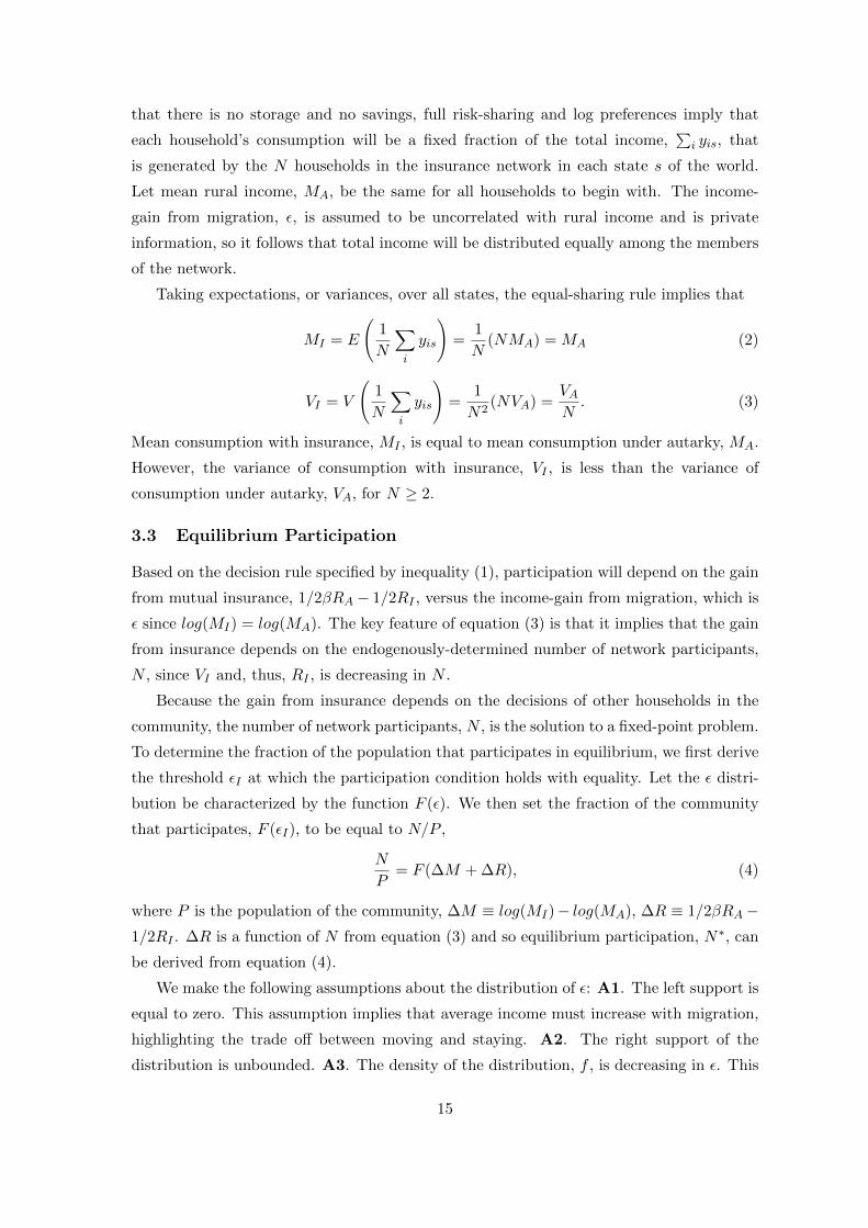
that there is no storage and no savings, full risk-sharing and log preferences imply that

each household’s consumption will be a fixed fraction of the total income,∑i yis, that

is generated by the N households in the insurance network in each state s of the world.

Let mean rural income, MA, be the same for all households to begin with. The income-

gain from migration, ε, is assumed to be uncorrelated with rural income and is private

information, so it follows that total income will be distributed equally among the members

of the network.

Taking expectations, or variances, over all states, the equal-sharing rule implies that

MI = E

(1

N

∑i

yis

)=

1

N(NMA) = MA (2)

VI = V

(1

N

∑i

yis

)=

1

N2(NVA) =

VAN. (3)

Mean consumption with insurance, MI , is equal to mean consumption under autarky, MA.

However, the variance of consumption with insurance, VI , is less than the variance of

consumption under autarky, VA, for N ≥ 2.

3.3 Equilibrium Participation

Based on the decision rule specified by inequality (1), participation will depend on the gain

from mutual insurance, 1/2βRA − 1/2RI , versus the income-gain from migration, which is

ε since log(MI) = log(MA). The key feature of equation (3) is that it implies that the gain

from insurance depends on the endogenously-determined number of network participants,

N , since VI and, thus, RI , is decreasing in N .

Because the gain from insurance depends on the decisions of other households in the

community, the number of network participants, N , is the solution to a fixed-point problem.

To determine the fraction of the population that participates in equilibrium, we first derive

the threshold εI at which the participation condition holds with equality. Let the ε distri-

bution be characterized by the function F (ε). We then set the fraction of the community

that participates, F (εI), to be equal to N/P ,

N

P= F (∆M + ∆R), (4)

where P is the population of the community, ∆M ≡ log(MI)− log(MA), ∆R ≡ 1/2βRA−1/2RI . ∆R is a function of N from equation (3) and so equilibrium participation, N∗, can

be derived from equation (4).

We make the following assumptions about the distribution of ε: A1. The left support is

equal to zero. This assumption implies that average income must increase with migration,

highlighting the trade off between moving and staying. A2. The right support of the

distribution is unbounded. A3. The density of the distribution, f , is decreasing in ε. This

15

assumption says that superior urban opportunities occur less frequently in the population.

Given these distributional assumptions,

Lemma 1. Equilibrium participation is characterized by a unique fixed point, N∗ ∈ (0, P ).

∆M = 0 because MI = MA. ∆R > 0 by assumption. This implies, from assumption

A1, that F (∆M + ∆R) > N/P at N = 0. Assumption A2 implies that F (∆M + ∆R) <

N/P at N = P . F (∆M+∆R) is increasing in N because RI is decreasing in N (hence, ∆R

must be increasing in N). By a continuity argument, a fixed point N∗ at which equation

(4) is satisfied must exist. We show in the Appendix that assumption A3 implies that

F (∆M + ∆R) is strictly concave, ensuring that this fixed point is unique.

3.4 Participation and Income-Sharing with Inequality

We now characterize equilibrium participation and the income-sharing rule with heteroge-

neous rural incomes. By introducing this realistic feature of communities, we are able to

derive an important implication of our theory, which is that relatively wealthy households

within the community will be more likely to send members to the city. To derive the new

equilibrium, we take advantage of the fact that the ratio of marginal utilities between any

two households participating in the network must be the same in all states of the world

with full risk-sharing. Dividing the community into K income classes of equal size, Pk, this

implies, given log preferences, that Cks/CKs = λk, where Cks, CKs denote the consumption

of households in income class k and K (the highest income class) in state s of the world.

Aggregating over all households who choose to participate in the network – Nk in each

income class k – each household in income class k consumes a fraction λk/∑k λkNk of the

total income,∑i yis, that is generated by the insurance network in each state of the world.

Note that we normalize so that λK equals one. Following the same steps as in equations

(2) and (3), expressions for the mean and variance of consumption with insurance in each

income class k are derived as follows:

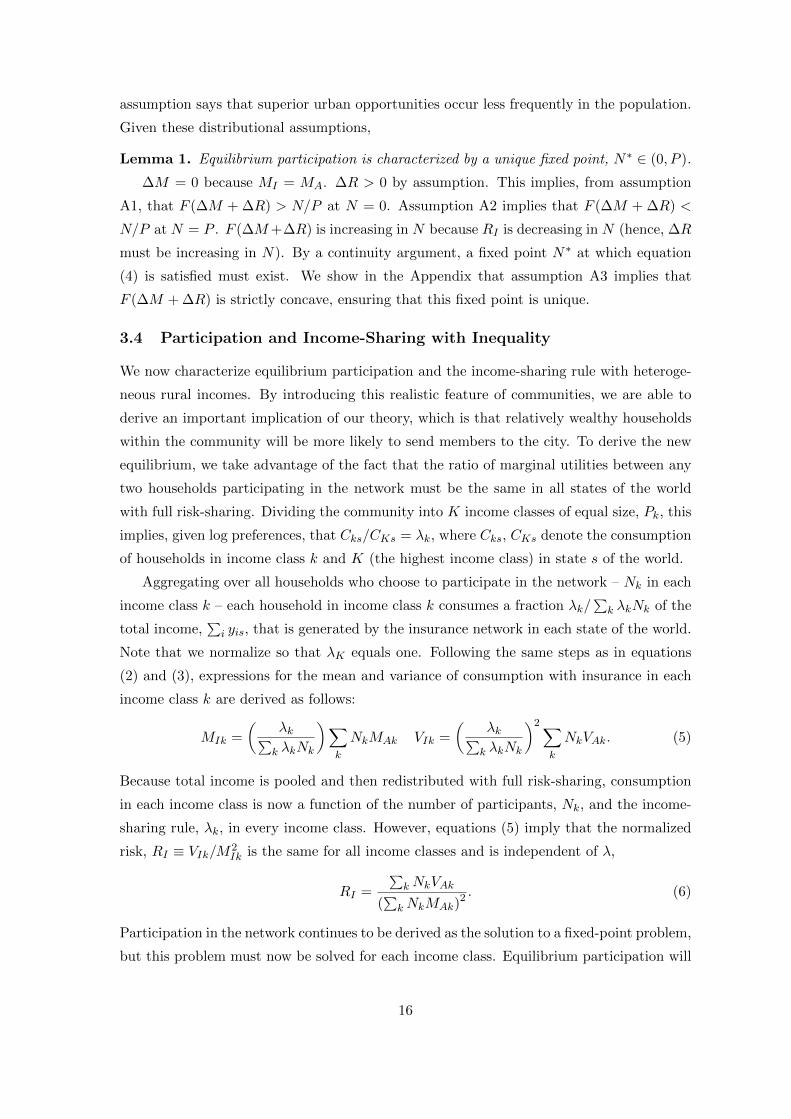
MIk =

(λk∑k λkNk

)∑k

NkMAk VIk =

(λk∑k λkNk

)2∑k

NkVAk. (5)

Because total income is pooled and then redistributed with full risk-sharing, consumption

in each income class is now a function of the number of participants, Nk, and the income-

sharing rule, λk, in every income class. However, equations (5) imply that the normalized

risk, RI ≡ VIk/M2Ik is the same for all income classes and is independent of λ,

RI =

∑kNkVAk

(∑kNkMAk)

2 . (6)

Participation in the network continues to be derived as the solution to a fixed-point problem,

but this problem must now be solved for each income class. Equilibrium participation will

16

satisfy the following conditions, corresponding to equation (4), for each income class k:

Nk

Pk= F (∆Mk + ∆Rk), (7)

where ∆Mk ≡ log(MIk)− log(MAk), ∆Rk ≡ 1/2βRAk − 1/2RI .

If we knew the income-sharing rule, λk, we could substitute expressions from equations

(5) and (6) in equation (7) to solve simultaneously for Nk in all K income classes. The more

challenging problem that we face is that the sharing-rule λk and participation Nk must be

derived simultaneously. To derive the sharing rule that is chosen by the community, we

assume that its objective is to maximize the surplus that is generated by the insurance

network. This surplus is the utility from participation in the network minus the utility in

autarky, summed over all income classes. Within each income class, k, the total number

of participants is determined by a threshold εIk = ∆Mk + ∆Rk. Households with ε > εIk

would send members to the city regardless of whether or not the insurance network was in

place. They can thus be ignored when computing the surplus generated by the network. If

β < 1, and given that ε > 0, households with ε < εIk will always send members to the city

when the network is absent. Total surplus can then be described by the expression,

W =∑k

Pk

∫ εIk

0

{[log(MIk)−

1

2RI

]−[log(MAk)−

1

2βRAk + ε

]}f(ε)dε.

Noting that Nk = Pk∫ εIk

0 f(ε)dε and collecting terms, the surplus function reduces to23

W =∑k

NkεIk − Pk∫ εIk

0εf(ε)dε. (8)

Equilibrium participation and the income-sharing rule can be jointly derived by maximiz-

ing W with respect to λk, subject to the fixed point conditions in equations (7), after

substituting in the expressions for MIk, RI from equations (5) and (6). We now use this

theoretical framework to identify which households benefit less (more) from the network

and who should therefore be more (less) likely to have migrant members.

3.5 Relative Wealth, Rural Risk, and Migration

If participation in the network were fixed, the community could increase the surplus gener-

ated by the network by redistributing income from richer households to poorer households

(given diminishing marginal utility). If households can select out of the network, how-

ever, the sharing-rule must be attentive to the possibility that increased exit by households

23If β > 1, then there exists a threshold ε, 0 < εAk < εIk, below which households do not send migrantsto the city even when the network is absent. The second term in square brackets in the preceding equationis then replaced by

∫ εAk

olog(MAk) − 1/2βRAk +

∫ εIkεAk

log(MAk) − 1/2βRAk + ε. We would then integrate

from εAk to εIk, rather than from zero to εIk, in equation (8). This would not, however, change any of theresults that follow.

17

who subsidize the rest of the network will make it smaller, reducing its ability to smooth

consumption. We nevertheless obtain the following result.

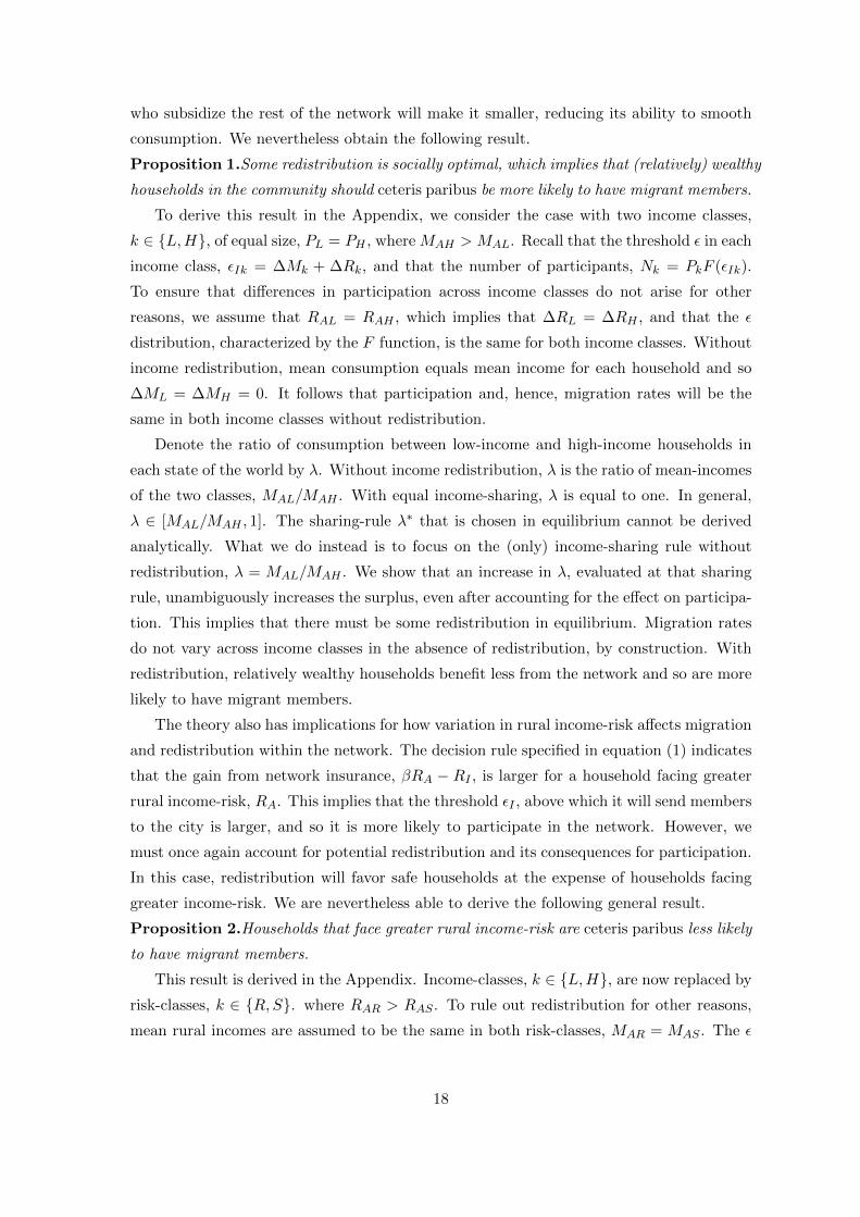
Proposition 1.Some redistribution is socially optimal, which implies that (relatively) wealthy

households in the community should ceteris paribus be more likely to have migrant members.

To derive this result in the Appendix, we consider the case with two income classes,

k ∈ {L,H}, of equal size, PL = PH , where MAH > MAL. Recall that the threshold ε in each

income class, εIk = ∆Mk + ∆Rk, and that the number of participants, Nk = PkF (εIk).

To ensure that differences in participation across income classes do not arise for other

reasons, we assume that RAL = RAH , which implies that ∆RL = ∆RH , and that the ε

distribution, characterized by the F function, is the same for both income classes. Without

income redistribution, mean consumption equals mean income for each household and so

∆ML = ∆MH = 0. It follows that participation and, hence, migration rates will be the

same in both income classes without redistribution.

Denote the ratio of consumption between low-income and high-income households in

each state of the world by λ. Without income redistribution, λ is the ratio of mean-incomes

of the two classes, MAL/MAH . With equal income-sharing, λ is equal to one. In general,

λ ∈ [MAL/MAH , 1]. The sharing-rule λ∗ that is chosen in equilibrium cannot be derived

analytically. What we do instead is to focus on the (only) income-sharing rule without

redistribution, λ = MAL/MAH . We show that an increase in λ, evaluated at that sharing

rule, unambiguously increases the surplus, even after accounting for the effect on participa-

tion. This implies that there must be some redistribution in equilibrium. Migration rates

do not vary across income classes in the absence of redistribution, by construction. With

redistribution, relatively wealthy households benefit less from the network and so are more

likely to have migrant members.

The theory also has implications for how variation in rural income-risk affects migration

and redistribution within the network. The decision rule specified in equation (1) indicates

that the gain from network insurance, βRA − RI , is larger for a household facing greater

rural income-risk, RA. This implies that the threshold εI , above which it will send members

to the city is larger, and so it is more likely to participate in the network. However, we

must once again account for potential redistribution and its consequences for participation.

In this case, redistribution will favor safe households at the expense of households facing

greater income-risk. We are nevertheless able to derive the following general result.

Proposition 2.Households that face greater rural income-risk are ceteris paribus less likely

to have migrant members.

This result is derived in the Appendix. Income-classes, k ∈ {L,H}, are now replaced by

risk-classes, k ∈ {R,S}. where RAR > RAS . To rule out redistribution for other reasons,

mean rural incomes are assumed to be the same in both risk-classes, MAR = MAS . The ε

18

distribution is also assumed to be the same in both classes. Relabel λ to be the ratio of

consumption between high-risk and low-risk households in each state of the world. Without

redistribution, λ = MAR/MAS = 1. If the two risk-classes are of equal size, PR = PS , then

the number of network participants will be greater in the risky class, NR > NS , because

∆MR = ∆MS = 0, ∆RR > ∆RS . The benefit of redistribution is that a dollar taken

from each participating risky household will be divided among a smaller number of safe

households. At the same time, the number of households that benefit is smaller than the

number who lose and this will be accounted for when computing the surplus. The effect of

redistribution on overall participation, with its consequences for consumption-smoothing,

must also be considered.

If there are net gains from redistribution, nevertheless, then λ will decline. However,

since the gains from redistribution arise because NR > NS , λ must be bounded below at a

level λ at which participation is the same in both risk classes; λ ∈ [λ, 1]. To prove Proposi-

tion 2 we focus on the (only) income-sharing rule with equal participation, λ = λ, and show

that an increase in λ evaluated at λ, unambiguously increases the surplus. This implies

that λ∗ > λ and, hence, that households facing greater rural income-risk have higher par-

ticipation rates (lower migration rates) in equilibrium even with redistribution. In contrast,

if networks are absent and we maintain the standard risk-diversification assumption, β < 1,

then households facing greater rural income-risk will be more likely to send migrants to the

city.24

4 Testing the Theory

The theory generates three testable predictions: (i) income is redistributed in favor of

poor households within the caste, (ii) relatively wealthy households who, therefore, benefit

less from the insurance network should be more likely to have migrant members, and (iii)

households facing greater rural income-risk who benefit more from the network should be

less likely to have migrant members. These tests shed light on the central hypothesis that

insurance provided by rural networks inhibits mobility. Additional tests validate the key

assumption that permanent male migration is associated with a loss in network services.

These results, taken together, can be used to distinguish between our explanation for large

24The available evidence supports the assumption that β < 1. As noted in Section 2, the NSS dataindicate that there is lower unemployment in urban versus rural areas in India. Everything else equal,this implies that income-risk declines with migration. β will certainly be less than one in that case, andthis is what we obtain when we estimate the structural parameters of the model. Without rural insurancenetworks, a household will not send migrants to the city if log(MA) − 1

2RA ≥ log(MA) − 1

2βRA + ε. If

β < 1, and we continue to assume ε > 0, then all households will send migrants, which is inconsistent withProposition 2. Once we introduce a migration cost, K, there exists a threshold ε∗ = K− 1

2(1−β)RA, above

which households send migrants. ε∗ is decreasing in RA, establishing a positive relationship between ruralincome-risk and migration in the absence of rural insurance networks that runs counter to Proposition 2once again.

19

wage gaps and low migration in India and alternative explanations that do not require a

role for rural insurance networks.

One explanation for low migration and large wage gaps in India is based on the existence

of urban caste-based labor market networks. While the members of a relatively small

number of castes with well-established urban networks will enjoy high wages in the city,

most potential migrants moving independently will be shut out of the urban labor market.

Past research; e.g. Munshi and Rosenzweig (2006), Munshi (2011), indicates that caste

networks continue to be active in Indian cities. However, this does not preclude the co-

existence of our theory, in which the loss in rural insurance reduces individual migration,

with this alternative explanation in which migrants must move as a group, which results

in lower overall mobility. Two distinguishing features of our theory are (i) that households

facing greater rural income-risk are less likely to have migrant members, and (ii) that

migration is associated with a loss in network services.25

There also can be alternative explanations for the first two predictions of our theory,

but no alternative that we are aware of delivers all three predictions. For example, it is

possible that communities provide other types of public goods financed by a progressive

payment scheme, also resulting in redistribution and increased exit by relatively wealthy

households.26 Moreover, there may be other reasons why higher household income, which

is positively correlated with relative income within the community, will be associated with

higher out-migration. Neither of these theories would explain why households facing greater

rural income-risk are less likely to have migrant members.

4.1 Evidence on Redistribution within Castes

We first empirically assess the extent of redistribution within castes. We begin with data

from the 2005-2011 Indian ICRISAT panel survey, which provides information on household

incomes over a seven-year period and consistent consumption data for the first four of

those years, for a sample of households in six villages in the states of Andhra Pradesh

and Maharashtra. The panel data enables us to compute the theoretically-relevant inter-

temporal mean values for consumption and income for each household.27

25Another explanation for low mobility, as in the literature on kin-tax in Africa; e.g. Platteau (2000), isthat origin networks tax migrants heavily. However, this would not explain why greater rural income-riskis associated with lower migration.

26Recent evidence from developing countries suggests that while payment schemes in rural communities areindeed redistributive, they are regressive rather than progressive (Olken and Singhal 2011). The empiricalevidence thus runs counter to this alternative explanation.

27These data provide the value of all foods and non-foods consumed, including self-produced and pur-chased items measured at various times over the year, that can be summed to obtain an annual total. TheIndian CPI for agricultural laborers is used to compute real consumption values expressed in 2005 rupees.Average real (inflation-adjusted) annual income is also computed for the same households over the entireseven-year period, including wages, salaries, and farm and non-farm income, but excluding any transfersand remittances.

20

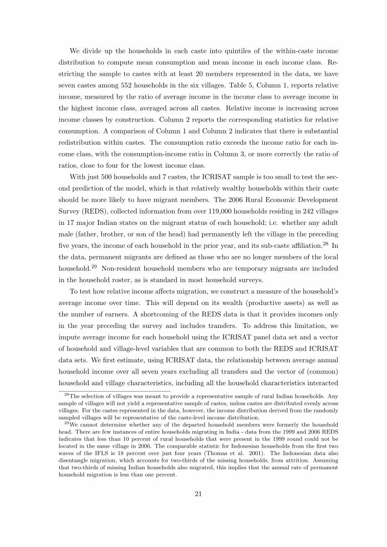
We divide up the households in each caste into quintiles of the within-caste income

distribution to compute mean consumption and mean income in each income class. Re-

stricting the sample to castes with at least 20 members represented in the data, we have

seven castes among 552 households in the six villages. Table 5, Column 1, reports relative

income, measured by the ratio of average income in the income class to average income in

the highest income class, averaged across all castes. Relative income is increasing across

income classes by construction. Column 2 reports the corresponding statistics for relative

consumption. A comparison of Column 1 and Column 2 indicates that there is substantial

redistribution within castes. The consumption ratio exceeds the income ratio for each in-

come class, with the consumption-income ratio in Column 3, or more correctly the ratio of

ratios, close to four for the lowest income class.

With just 500 households and 7 castes, the ICRISAT sample is too small to test the sec-

ond prediction of the model, which is that relatively wealthy households within their caste

should be more likely to have migrant members. The 2006 Rural Economic Development

Survey (REDS), collected information from over 119,000 households residing in 242 villages

in 17 major Indian states on the migrant status of each household; i.e. whether any adult

male (father, brother, or son of the head) had permanently left the village in the preceding

five years, the income of each household in the prior year, and its sub-caste affiliation.28 In

the data, permanent migrants are defined as those who are no longer members of the local

household.29 Non-resident household members who are temporary migrants are included

in the household roster, as is standard in most household surveys.

To test how relative income affects migration, we construct a measure of the household’s

average income over time. This will depend on its wealth (productive assets) as well as

the number of earners. A shortcoming of the REDS data is that it provides incomes only

in the year preceding the survey and includes transfers. To address this limitation, we

impute average income for each household using the ICRISAT panel data set and a vector

of household and village-level variables that are common to both the REDS and ICRISAT

data sets. We first estimate, using ICRISAT data, the relationship between average annual

household income over all seven years excluding all transfers and the vector of (common)

household and village characteristics, including all the household characteristics interacted

28The selection of villages was meant to provide a representative sample of rural Indian households. Anysample of villages will not yield a representative sample of castes, unless castes are distributed evenly acrossvillages. For the castes represented in the data, however, the income distribution derived from the randomlysampled villages will be representative of the caste-level income distribution.

29We cannot determine whether any of the departed household members were formerly the householdhead. There are few instances of entire households migrating in India - data from the 1999 and 2006 REDSindicates that less than 10 percent of rural households that were present in the 1999 round could not belocated in the same village in 2006. The comparable statistic for Indonesian households from the first twowaves of the IFLS is 18 percent over just four years (Thomas et al. 2001). The Indonesian data alsodisentangle migration, which accounts for two-thirds of the missing households, from attrition. Assumingthat two-thirds of missing Indian households also migrated, this implies that the annual rate of permanenthousehold migration is less than one percent.

21

with mean rainfall. The vector of regressors have sufficient predictive power, given that

this is a cross-sectional regression, with an R-squared around 0.3. The coefficients obtained

from the regression estimated with ICRISAT data are then used to impute average income

for each of the REDS households, based on their characteristics.30

As noted, the ICRISAT villages are located in Andhra Pradesh and Maharashtra.

For comparability, we restricted the REDS sample to four geographically contiguous and

broadly similar South Indian states – Maharashtra, Andhra Pradesh, Tamil Nadu, and Kar-

nataka – when imputing incomes.31 Average consumption is also imputed for the REDS

households from ICRISAT consumption data using the same method and the same first-

stage specification that was used to impute average income. Table 5, Columns 4-6 replicate

the computations carried out with the ICRISAT data for the REDS sample. A comparison

of Column 4 and Column 5 indicates that, as is true for the ICRISAT households (where

no values are imputed), there is substantial redistribution within castes. The consumption

ratio exceeds the income ratio for each income class, with the consumption-income ratio in

Column 6, or more correctly the ratio of ratios, close to three for the lowest income class.

Finally, Column 7 reports migration rates by income class. Consistent with the theory

and the redistribution documented in Table 5, we see that migration rates are increasing in

relative income. A household’s relative position within its caste’s income distribution will

be positively correlated with its absolute income. The statistics reported in Column 7 do

not account for the direct effect of (absolute) household income on migration, which would

dampen the increase in migration across relative income classes if wealthier households are

less likely to migrate for other reasons. The regression analysis that follows will control for

the direct effect of the household’s income on migration.

30Both data sets provide household-level information on total land area (together with a binary variableindicating whether the household is landless), irrigated area, soil type (red, black, sandy) and soil depth,household size, the number of earners, and the occupation of the household head. Each data set alsoprovides, at the village level, a time-series of rainfall; daily rainfall for all seven years for the ICRISATsurvey and monthly data over an eight-year period starting in 1999 for the REDS, from which we constructvillage-level mean annual rainfall and the variance of annual rainfall. When imputing average income forREDS households with permanent male migrants, we included those migrants among the earners. Theland characteristics, taken together, determine the value of land owned by the household. Although landwealth accounts for 85% of household wealth in rural India (Rosenzweig and Wolpin 1993), land salesare extremely infrequent (Foster and Rosenzweig 2002). This implies that land wealth is largely inheritedand can be treated as predetermined, at least from the perspective of current household members. Thehousehold’s permanent labor income is determined by the number of earners and the occupation of thehousehold head. Occupational choices are very limited in rural India. In the 2006 REDS census, 34% of theheads were cultivators; i.e. landowners and 38% were agricultural laborers and laborers not classified. Thenext most popular occupation shopkeepers accounted for just 2% of the household heads. Not surprisingly,the most important determinants of household income are landholding size and number of male earners.

31The advantage of including Karnataka and Tamil Nadu is that they increase the number of observations,particularly in the structural estimation where households are aggregated by income class in each caste.The reduced-form results reported below are largely unchanged and statistically significant when the sampleis restricted to the non-ICRISAT states (Karnataka and Tamil Nadu).

22

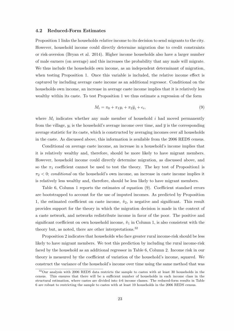
4.2 Reduced-Form Estimates

Proposition 1 links the households relative income to its decision to send migrants to the city.

However, household income could directly determine migration due to credit constraints

or risk-aversion (Bryan et al. 2014). Higher income households also have a larger number

of male earners (on average) and this increases the probability that any male will migrate.

We thus include the households own income, as an independent determinant of migration,

when testing Proposition 1. Once this variable is included, the relative income effect is

captured by including average caste income as an additional regressor. Conditional on the

households own income, an increase in average caste income implies that it is relatively less

wealthy within its caste. To test Proposition 1 we thus estimate a regression of the form

Mi = π0 + π1yi + π2yi + εi, (9)

where Mi indicates whether any male member of household i had moved permanently

from the village, yi is the household’s average income over time, and y is the corresponding

average statistic for its caste, which is constructed by averaging incomes over all households

in the caste. As discussed above, this information is available from the 2006 REDS census.

Conditional on average caste income, an increase in a household’s income implies that

it is relatively wealthy and, therefore, should be more likely to have migrant members.

However, household income could directly determine migration, as discussed above, and

so the π1 coefficient cannot be used to test the theory. The key test of Proposition1 is

π2 < 0; conditional on the household’s own income, an increase in caste income implies it

is relatively less wealthy and, therefore, should be less likely to have migrant members.

Table 6, Column 1 reports the estimates of equation (9). Coefficient standard errors

are bootstrapped to account for the use of imputed incomes. As predicted by Proposition

1, the estimated coefficient on caste income, π̂2, is negative and significant. This result

provides support for the theory in which the migration decision is made in the context of

a caste network, and networks redistribute income in favor of the poor. The positive and

significant coefficient on own household income, π̂1 in Column 1, is also consistent with the

theory but, as noted, there are other interpretations.32

Proposition 2 indicates that households who face greater rural income-risk should be less

likely to have migrant members. We test this prediction by including the rural income-risk

faced by the household as an additional regressor in Table 6, Column 2. Income risk in our

theory is measured by the coefficient of variation of the household’s income, squared. We

construct the variance of the household’s income over time using the same method that was

32Our analysis with 2006 REDS data restricts the sample to castes with at least 30 households in thecensus. This ensures that there will be a sufficient number of households in each income class in thestructural estimation, where castes are divided into 4-6 income classes. The reduced-form results in Table6 are robust to restricting the sample to castes with at least 10 households in the 2006 REDS census.

23

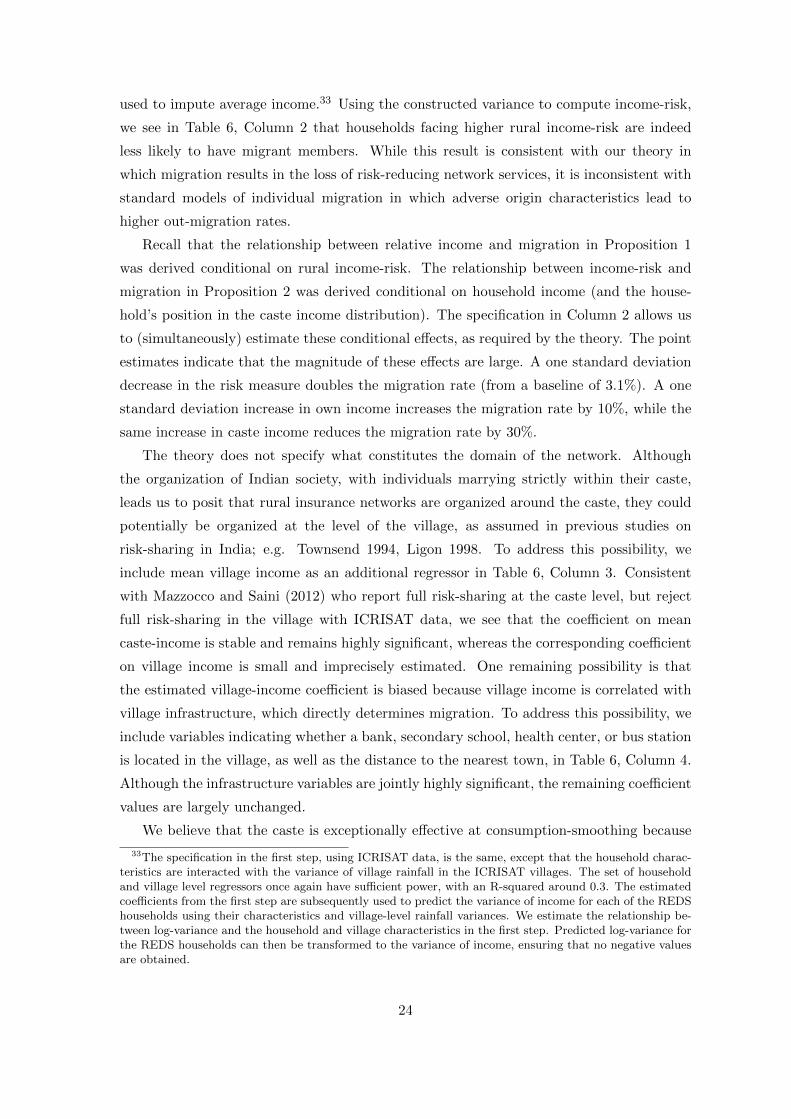
used to impute average income.33 Using the constructed variance to compute income-risk,

we see in Table 6, Column 2 that households facing higher rural income-risk are indeed

less likely to have migrant members. While this result is consistent with our theory in

which migration results in the loss of risk-reducing network services, it is inconsistent with

standard models of individual migration in which adverse origin characteristics lead to

higher out-migration rates.

Recall that the relationship between relative income and migration in Proposition 1

was derived conditional on rural income-risk. The relationship between income-risk and

migration in Proposition 2 was derived conditional on household income (and the house-

hold’s position in the caste income distribution). The specification in Column 2 allows us

to (simultaneously) estimate these conditional effects, as required by the theory. The point

estimates indicate that the magnitude of these effects are large. A one standard deviation

decrease in the risk measure doubles the migration rate (from a baseline of 3.1%). A one

standard deviation increase in own income increases the migration rate by 10%, while the

same increase in caste income reduces the migration rate by 30%.

The theory does not specify what constitutes the domain of the network. Although

the organization of Indian society, with individuals marrying strictly within their caste,

leads us to posit that rural insurance networks are organized around the caste, they could

potentially be organized at the level of the village, as assumed in previous studies on

risk-sharing in India; e.g. Townsend 1994, Ligon 1998. To address this possibility, we

include mean village income as an additional regressor in Table 6, Column 3. Consistent

with Mazzocco and Saini (2012) who report full risk-sharing at the caste level, but reject

full risk-sharing in the village with ICRISAT data, we see that the coefficient on mean

caste-income is stable and remains highly significant, whereas the corresponding coefficient

on village income is small and imprecisely estimated. One remaining possibility is that

the estimated village-income coefficient is biased because village income is correlated with

village infrastructure, which directly determines migration. To address this possibility, we

include variables indicating whether a bank, secondary school, health center, or bus station

is located in the village, as well as the distance to the nearest town, in Table 6, Column 4.

Although the infrastructure variables are jointly highly significant, the remaining coefficient

values are largely unchanged.

We believe that the caste is exceptionally effective at consumption-smoothing because

33The specification in the first step, using ICRISAT data, is the same, except that the household charac-teristics are interacted with the variance of village rainfall in the ICRISAT villages. The set of householdand village level regressors once again have sufficient power, with an R-squared around 0.3. The estimatedcoefficients from the first step are subsequently used to predict the variance of income for each of the REDShouseholds using their characteristics and village-level rainfall variances. We estimate the relationship be-tween log-variance and the household and village characteristics in the first step. Predicted log-variance forthe REDS households can then be transformed to the variance of income, ensuring that no negative valuesare obtained.

24

of its large size and scope (extending over many villages). While the preceding results

indicate that insurance networks in India are organized around the caste, they do not tell

us whether the network extends beyond village boundaries. To answer this question, we

replace village income with the mean income of caste households within the village in Table

6, Column 5. Reassuringly, the complete caste-income coefficient maintains its size and

significance, while the restrictive caste-income measure has little effect on migration and

is statistically insignificant. The stability of the caste-income coefficient to the inclusion

of a vector of village-level variables indicates that the results are not being driven by

unobserved village-level effects.34 Nevertheless, as a final robustness test, we include a

full set of village fixed effects in Column 6. Although the caste-income coefficient is now

only statistically significant at the 12 percent level (one-tailed test), it remains as large

(in absolute magnitude) as it was with the benchmark specification in Column 2. Results

from a Hausman test (available from the authors) indicate that the difference in the caste

income coefficient between the benchmark specification and the specification with village

fixed effects is not significant at the 5 percent level. The difference between the household

income coefficients is also not statistically significant, at any level. The only statistically

significant change is for the income-risk coefficient, but that coefficient is highly significant

in both specifications (and gets more negative in the fixed effects specification). Overall, our

results provide strong support for the hypothesized trade-off between the insurance provided

by rural caste-based networks and the income-gain from migration. Those households that

benefit less (more) from the rural network are more (less) likely to have migrant members.

4.3 Structural Estimates

Having found evidence consistent with the theory, we now estimate the structural param-

eters of the model. The structural estimates are used to (i) externally validate the model,

(ii) to provide independent support for the redistribution within castes that is predicted by

the theory, and (iii) to carry out counter-factual simulations that compare the sensitivity

of migration to the rural-urban wage gap and formal insurance. We also conduct counter-

factual policy simulations that quantify the mobility-enhancing effects of a government

safety net for poor households and a credit scheme benefiting wealthy households.

There are two exogenous variables in the model, measured at the level of the income-

class, k: mean-income, MAk, and normalized risk, RAk ≡ VAk/M2Ak. While there is a

single caste (community) in the theoretical analysis, there are 100 castes in the 2006 REDS

census, which we use for the structural estimation. To be consistent with the model, we

thus proceed to average mean-income, MAi, and the variance of income, VAi, which were

previously imputed for each household i, across all household in each income-class, k,

34Standard errors in Columns 3-5 are two-way clustered at the level of the caste and the village.

25

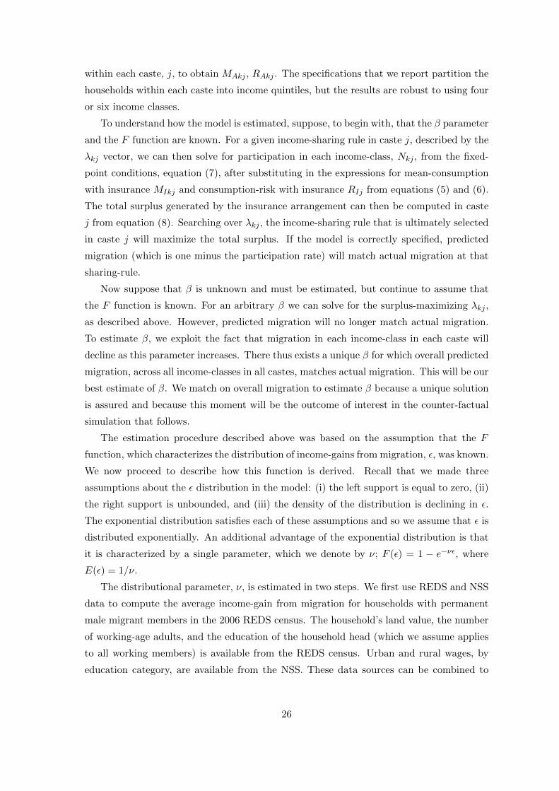
within each caste, j, to obtain MAkj , RAkj . The specifications that we report partition the

households within each caste into income quintiles, but the results are robust to using four

or six income classes.

To understand how the model is estimated, suppose, to begin with, that the β parameter

and the F function are known. For a given income-sharing rule in caste j, described by the

λkj vector, we can then solve for participation in each income-class, Nkj , from the fixed-

point conditions, equation (7), after substituting in the expressions for mean-consumption

with insurance MIkj and consumption-risk with insurance RIj from equations (5) and (6).

The total surplus generated by the insurance arrangement can then be computed in caste

j from equation (8). Searching over λkj , the income-sharing rule that is ultimately selected

in caste j will maximize the total surplus. If the model is correctly specified, predicted

migration (which is one minus the participation rate) will match actual migration at that

sharing-rule.

Now suppose that β is unknown and must be estimated, but continue to assume that

the F function is known. For an arbitrary β we can solve for the surplus-maximizing λkj ,

as described above. However, predicted migration will no longer match actual migration.

To estimate β, we exploit the fact that migration in each income-class in each caste will

decline as this parameter increases. There thus exists a unique β for which overall predicted

migration, across all income-classes in all castes, matches actual migration. This will be our

best estimate of β. We match on overall migration to estimate β because a unique solution

is assured and because this moment will be the outcome of interest in the counter-factual

simulation that follows.

The estimation procedure described above was based on the assumption that the F

function, which characterizes the distribution of income-gains from migration, ε, was known.

We now proceed to describe how this function is derived. Recall that we made three

assumptions about the ε distribution in the model: (i) the left support is equal to zero, (ii)

the right support is unbounded, and (iii) the density of the distribution is declining in ε.

The exponential distribution satisfies each of these assumptions and so we assume that ε is

distributed exponentially. An additional advantage of the exponential distribution is that

it is characterized by a single parameter, which we denote by ν; F (ε) = 1 − e−νε, where

E(ε) = 1/ν.

The distributional parameter, ν, is estimated in two steps. We first use REDS and NSS

data to compute the average income-gain from migration for households with permanent

male migrant members in the 2006 REDS census. The household’s land value, the number

of working-age adults, and the education of the household head (which we assume applies

to all working members) is available from the REDS census. Urban and rural wages, by

education category, are available from the NSS. These data sources can be combined to

26

compute the income-gain from migration, ε̃, and its utility equivalent, ε = log(1 + ε̃).35 We

assume that this derived income-gain, ε, is the representative (median) value for households

with migrants. For example, if 4 percent of households have permanent migrant members,

then ε applies to a household at the 98th percentile of the ε distribution. This assumption,

together with the properties of the exponential distribution, can be used to derive the

distributional parameter:

ν =−log(x/200)

ε, (10)

where x equals four in the preceding example. Once ν is computed, the risk-parameter, β,

can be estimated as described above.

As a basis for comparison with the estimates that follow, Table 7, Columns 1-2 list

relative consumption and migration in each of the five relative income-classes (averaged

across all castes). Columns 3-4, report the β estimate, predicted relative consumption, λk,

and predicted migration, 1−Nk/Pk, in each of those classes, k (once again averaged across

all castes, j). Jack-knifed standard errors, constructed by removing one caste at a time

and re-estimating the model, are reported in parentheses.36 The point-estimate for the β

parameter is 1.4. Similar results are obtained with four and six income-classes in Appendix

Table A3. β < 1 if migration reduces income-risk, as commonly assumed. We will see

momentarily that β does decline below one, and is much more precisely estimated, with a

flexible specification of the model that does a better job of matching the data.

The β parameter is estimated by matching on overall migration, which is 4.3 percent.

Notice, however, that migration rates predicted by the model are lower (higher) than actual

migration rates in low (high) income classes. In contrast, relative consumption levels (λ’s)

predicted by the model match closely with actual relative consumption. We cannot reject

that predicted and actual relative consumption are statistically equal, at conventional lev-

els, in each income class and across all specifications in Table 7. The match in terms of

magnitudes is very close (less than 5 percent error for each income-class with the benchmark

specification with a single ν).37 This close match in predicted and actual λ’s is effectively a

35We compute average rural income as 5 percent of the household’s total asset holdings at the beginningof the reference period (one year before the survey round) plus labor income, based on the assumption thatthe adults in the household work for 312 days in the year. Let V be the household’s asset value, L thenumber of adults, and WU , WR the education-adjusted urban and rural wages from the NSS. The averagenumber of working-age adults per household in the 2006 REDS census is 1.4, and so it is reasonable toassume that a single individual migrates. The income-gain from migration in that case is 312(WU−WR)

0.05V+312WRL.

This statistic is averaged across all households with migrants.36The jack-knifed standard error for any parameter θ is given by the expression [n/n− 1

∑i(θi − θ)2]1/2,

where n is the number of times the model is re-estimated, θi is the parameter estimate when it is re-estimatedfor the ith time, and θ is the average across all θi. In our case, with 100 castes, n = 100.

37An alternative approach to compare the closeness of the match, suggested by a referee, would be tocompute the probability that the predicted and actual λ’s are as close as they are by random chance. Weimplement this test for the lowest relative income-class, since it will certainly not subsidize any other income-class and so the range of feasible λ’s is known. Given that the relative income for the lowest income-classis 0.31 from Table 5, λ must lie in [0.31, 1]. If the predicted λ is distributed uniformly over this range, theprobability that it will lie within 0.04 of the actual λ, as observed for the benchmark specification in Table

27

test of external validity, given that consumption data are not used to estimate the model.

It provides empirical support for both the (logarithmic) distributional assumption and our

use of a utilitarian social welfare function, placing equal weight on all income classes in

equation (8). The substantial redistribution documented in Table 5 appears to be driven

entirely by an attempt to equate marginal utilities across income classes.

One possible explanation for the mismatch between predicted and actual migration

across income classes is that the income-gain from migration varies with rural income,

perhaps because members of wealthier households are better educated. Although the theo-

retical analysis assumes that the (proportional) income-gain is independent of rural income,

we relax this assumption when estimating the model in Table 7, Columns 5-6. The house-

holds in the 2006 REDS census are divided into five absolute income classes, without regard

to their caste affiliation, and the ν parameter is then computed in each income class using

the procedure described above.38 Each relative income-class k in caste j can be mapped

into an absolute income-class based on its mean income, MAkj . The ν parameter com-

puted for that absolute income-class is then assigned to class k in caste j. The results with

this flexible specification in Columns 5-6 are very similar to the results obtained with the

benchmark specification in Columns 3-4. Allowing the income-gain from migration to vary

with rural income evidently does not reduce the mismatch between predicted and actual

migration.

Although the theory focuses on the constraints faced by individuals migrating indepen-

dently, the empirical analysis must take account of the small number of castes that have

established urban networks in the city. While most castes report low migration rates in our

data, a few do have substantial rates of permanent male migration. We account for these

caste-level differences by estimating a flexible specification that allows for a caste-specific

ν parameter. The income-gain computed for households with migrants ε, using REDS and

NSS data as described above, does not vary substantially across castes. The important

difference is the point in the ε distribution where these households are located. For a caste

with a strong network and many migrants, x in equation (10) is relatively large, which

implies that ν = 1/E(ε) will be small. A strong urban caste network, reflected in a high

level of permanent migration in the data, thus effectively increases the income-gain from

migration. Despite the flexibility that is introduced with 100 ν parameters, the pattern of

λ’s and migration in Columns 7-8 is very similar to the benchmark estimates obtained with

7, is 12 percent. The standard error for the lowest income class is also small enough for us to reject thatthere is no redistribution (λ is equal to 0.31) with greater than 95 percent confidence.

38Appendix Table A4 shows, with five absolute income-classes, that land value, the number of working-age adults, and the education of the household head are all generally increasing across income classes asexpected. Although the NSS data indicate that the rural-urban wage gap is increasing with education(Hnatkovskay and Lahiri 2013), wealthier households are starting from a higher rural income-base and sothe proportional gain in income will naturally be smaller for them. There is no obvious relationship betweenabsolute income and the income-gain from migration, which is reflected in the migration rate, in Table A4.

28

a single ν parameter. Notice that the β coefficient is now smaller than one, consistent with

the standard assumption that migration reduces income-risk, although it continues to be

imprecisely estimated.

We assumed, when deriving the theoretical results, that there was a single ν and a single

β. The specifications reported in Columns 5-8 relax the first assumption. We now relax the

second assumption by allowing β to vary with rural household income (there is no reason to

allow β to vary by caste if households with migrants are excluded from their rural insurance

networks). Recall that β reflects the income diversification that accompanies migration as

well as access to non-network consumption-smoothing mechanisms. It is not obvious how

the reduction in income-risk through migration varies with rural income. While we would

expect wealthier households to have greater access to private credit, the effect on β is

theoretically ambiguous. Consider, for example, two households trying to smooth their

consumption with credit, where one household has twice as much income as the other in

each state of the world. To smooth consumption completely, the wealthier household must

receive twice as much credit in each state of the world. If land, the chief source of wealth

in rural India, is not fully collateralizable, then this condition may or may not be satisfied

and the β-income relationship will be ambiguous.

The structural estimates in Table 7, Columns 9-10 allow β to be a linear function of

average income in each relative income-class within each caste; β = α + γMAkj , without

any theoretical guidance about the sign of the γ parameter. Empirically, predicted mi-

gration rates were too high (low) for higher (lower) relative income-classes with a single

β parameter. With the flexible specification, we thus expect the gamma coefficient to be

positive to bring predicted migration in line with actual migration. The estimated coeffi-

cients in Columns 9-10 are consistent with this prediction. Since there are two parameters

to estimate – α and γ – we match on two moments: overall migration in the lowest and

the highest relative income class.39 It is reassuring to observe that predicted and actual

migration now match closely in the remaining three income-classes. We are even able to

generate the non-monotonicity from relative income-classes three to five, despite the fact

that β is specified to be increasing linearly in mean-income MAkj , without regard to the

relative position of group k in caste j.

To compare the parameter estimates with the flexible specification with what we ob-

tained earlier in Columns 3-8, we use the estimated α and γ parameters to compute β for

the representative household with mean-wealth in the REDS census. Jack-knifed standard

errors for the β parameter are constructed using the procedure described above. The β

parameter with the preferred flexible specification now lies below one and is very precisely

estimated. If we take a different approach that exploits variation in household income in

39The standard errors for these two income classes in Column 10 simply reflect the sampling error thatis generated when we re-estimate the model, removing one caste at a time, in the jack-knife procedure.

29

the sample, then the β parameter would be less than one (based on the estimated α and γ

parameters) for 86 percent of the households in the REDS census. This result is consistent

with evidence from the NSS indicating that employment-risk is lower in urban than in rural

areas, which implies (everything else equal) that income-risk will be lower in urban areas.

The fact that households facing greater rural income-risk were nevertheless less likely to

have migrant members in Table 6, indicates that the loss in network insurance must be large

enough to dominate the substantial income-gain and the (possible) income risk-reduction

associated with migration.

Given that the structural model appears to fit the data reasonably well, we use the

estimated parameter values to perform counter-factual simulations that quantify the mag-

nitude of the mobility restrictions we have uncovered. There are two structural parameters

in the model: the risk parameter, β, and the income-gain parameter, ν. We reduce the β

parameter to assess the effect of an improvement in formal insurance on migration, taking

as given the rural insurance arrangements that are in place. We assess the sensitivity of

migration to changes in the income-gain from migration by increasing the ν parameter.

Figure 7 reports overall migration rates over a range of counter-factual β values, using

both the benchmark specification (single ν, single β) and the flexible specification (caste-

specific ν, β increasing in household income). A 50 percent decline in β, which is still quite

far from full insurance (β equal to zero) more than doubles the migration rate from 4 to 9

percent with the more precisely estimated flexible specification, highlighting the importance

of risk in restricting mobility. How responsive is migration to an exogenous change in the

income-gain from migration? Given historically low migration rates, despite the persistently

large wage gap in India, we would expect predicted migration to be insensitive to changes

in the income-gain if the model is correct. Counter-factual simulations in Figure 7 that

vary the value of the ν parameter, but retain the assumption that formal insurance is

unavailable, verify that this is indeed the case. An 80 percent increase in the ν parameter,

which corresponds to an average decline in the income-gain from 18 percent to 10 percent

lowers migration by just one percentage point. This result further emphasizes the central

message of this paper, which is that inadequate access to formal insurance, rather than

wage differentials as commonly assumed in models of migration, may explain much of the

low mobility in India.40

40Counterfactual simulations reported in Appendix Figure A1 shift the ν parameter in the oppositedirection. A 50% decline in the ν parameter, which corresponds to a doubling of the wage-gap from 18%to 36%, increases the migration rate by just 1.5% percentage points from a baseline of 4.3%. However,migration is much more responsive to the wage-gap, in absolute and relative terms, when the β parameteris halved from a baseline value of 1.4; migration increases from 6% to 9%.

30

4.4 Testing the Mechanism

The key assumption underlying our theory is that permanent male migration is associated

with a loss in network services. We test this assumption by examining how a house-

hold’s relative wealth affects three variables: out-migration, network participation, and

out-marriage. Recall that marriage within the caste is a prerequisite for participation in

the network.

Each REDS round consists of a census of households in the representative sample of

villages, followed by a detailed survey of a sample of households in those villages. The

survey collects information on permanent migration by adult males, as in the census. In

addition, it collects information on financial transactions wihin the caste, which directly

measures participation in the insurance network, as well as marriage within the caste by

household members.41

Although the number of households in the detailed survey is relatively small, a major

advantage over the census is that they can be linked over successive REDS rounds. We

thus construct a panel, using the surveyed households in the 1982 and 1999 rounds of the

REDS, for the joint test of the key theoretical assumption.42 We eliminate all castes with

less than 10 households in the REDS survey, and then proceed to estimate the following

equation:

Xit = π1yit + π2yit + fi + εit, (11)

where yit is household i’s average income in survey round t (1982, 1999), yit is the corre-

sponding caste average, and fi is a household fixed effect. This is the same specification as

equation (9), except that household fixed effects and time subscripts are included. Equation

(11) is separately estimated with out-migration, out-marriage, and network participation

as dependent variables.

Average household income, yit, could be determined by unobserved household attributes

that independently determine the outcomes of interest. These attributes could also be

correlated with caste income, yit, to the extent that they are correlated across households

within the caste. Differencing over the two years allows us to purge these fixed attributes,

∆Xit = π1∆yit + π2∆yit + ∆εit. (12)

41Participation in the caste network is measured by a binary variable that takes the value one if thehousehold sent or received caste-transfers (gifts or loans from one or more members of the same sub-caste)in the year preceding each survey round. The measures of out-marriage and out-migration are constructedfrom the 1999 retrospective histories on the marriages and migration of all of the siblings and childrenof each household head in the sample. From these histories we created a variable indicating whether anychild of the household head married outside the caste in the 10-year period prior to each survey date. Themeasure of out-migration is whether any male aged 20-30 at the time of each survey and residing in thehousehold prior to the survey had left the village permanently by the survey date.

42To construct the panel, we start with the sample of households in the 1982 round. Because of householdpartitioning, many 1982 household members were distributed across multiple households in 1999. We thusaggregate all 1999 households to be consistent with 1982 household boundaries, resulting in a balancedpanel over the two years.

31

However, shocks to income could still be correlated with unobserved changes in the de-

terminants of out-migration, out-marriage, and network participation ∆εit; for example, if

schools, banks, or other infrastructure that independently changed incomes and the out-

comes of interest were introduced in the household’s village between 1982 and 1999. To

address this concern, we construct instruments for ∆yit, ∆yit in equation (12) above.

We make use of two technological features of the Indian Green Revolution to construct

these instruments: (i) only certain parts of the country could profit from the new HYV

seeds at the onset of the Green Revolution in the late 1960s, and (ii) the returns to invest-

ing in the HYV technology are much greater on irrigated land. The instrumental variable

strategy allows for the possibility that initial availability of HYV technology and access to

irrigation were independently correlated with unobserved village and household character-

istics that had long-term effects on the outcomes of interest by including them in the second

stage. Exploiting the technological complementarity between HYV and irrigation, and the

fact that simultaneous access to these inputs was quasi-random, only the interaction of

these variables, measured in 1971, is used as an instrument for changes in income from

1982 to 1999.43 To add statistical power, we include two more instruments: the amount

of land inherited by the household head, as reported in the 1982 REDS round, and the

triple interaction of inherited wealth, HYV, and irrigation. The corresponding caste-level

instruments are the caste averages of the three household-level instruments.

The income variable that we construct depends on the household’s assets and the num-

ber of working age adults (including permanent migrants, if any). The same procedure was

used in the structural estimation to construct the income-gain from migration for house-

holds with migrants, except that we now use the village-level daily wage in the survey year

rather than the NSS wage to measure rural labor income. Caste-level income is once again

simply the caste average of household incomes. Note that we no longer need to impute

43This instrument is constructed by interacting a binary variable indicating whether anyone in householdi’s village used HYV in 1971 with the share of irrigated land in the village in that year. These variables areobtained from the 1971 REDS round, which is at the onset of the Green Revolution but still close enoughin time to predict changes in income over the 1982-1999 period. All areas of the country did not benefitequally from the HYV technology at the onset of the Green Revolution (see Munshi, 2004, for details). Theearly rice varieties, in particular, were unsuitable for cultivation in many areas, and it was only by cross-breeding with local varieties that the new technology could be adopted throughout the country. Althoughthe new wheat varieties were more robust, marketing was restricted to specific districts in the early stagesof the Green Revolution. Where the new HYV technology did become available, credit constraints wouldhave prevented growers from making the complementary investments in irrigation that were required toexploit the enhanced potential of the new seeds. Access to irrigation at that time would have been largelydetermined by proximity to water bodies and pre-existing irrigation technologies like tanks and canals,which was independent of the program priorities and technological constraints that determined access toHYV. The simultaneous access to HYV technology and irrigation, conditional on access to each of theseinputs separately, can thus be treated as quasi-random (satisfying the exclusion restriction). At the sametime, the combination of these inputs, net of their direct effects, would still have determined initial farmprofits due to the fact that the new HYV technology performed much better on irrigated land. Givencredit constraints, these initial profits would have determined the subsequently income trajectory and thisis indeed what we observe in the first-stage regression.

32

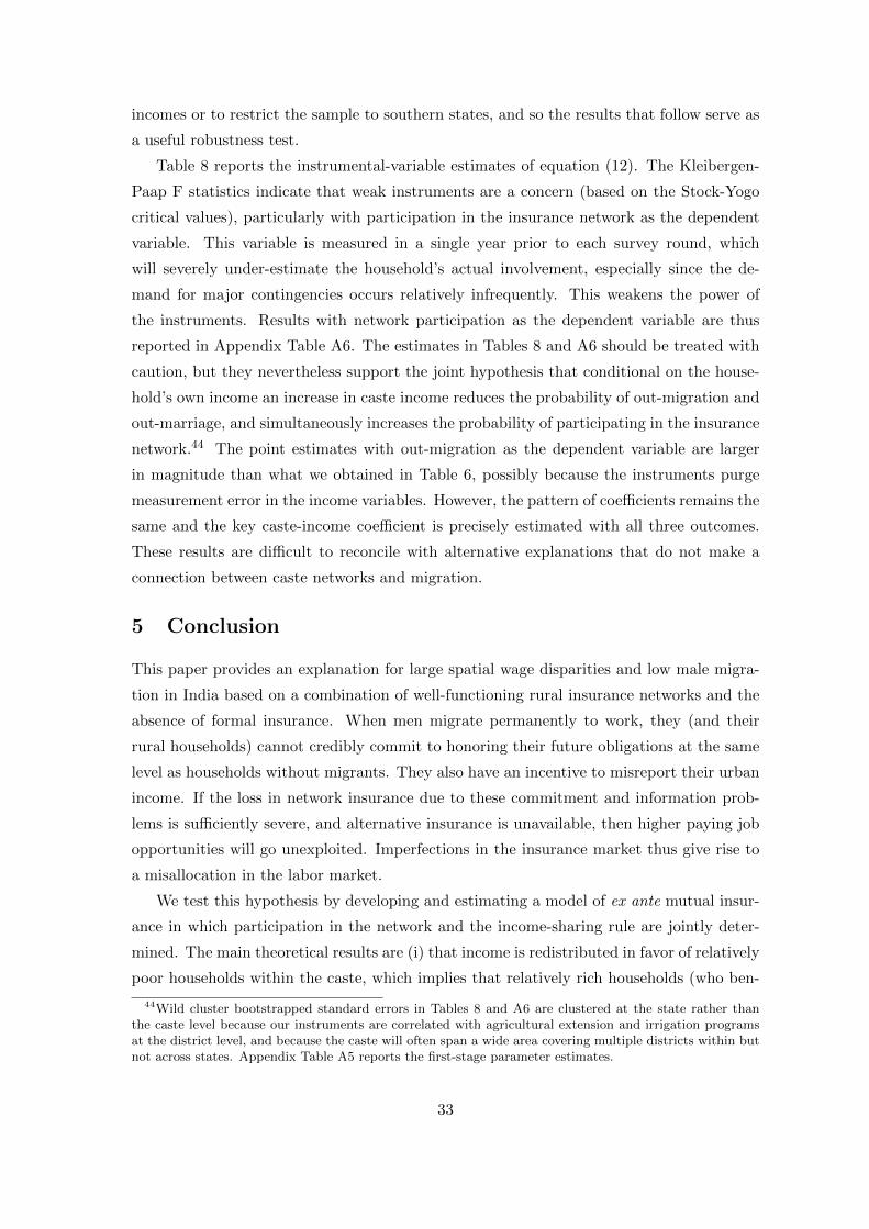
incomes or to restrict the sample to southern states, and so the results that follow serve as

a useful robustness test.

Table 8 reports the instrumental-variable estimates of equation (12). The Kleibergen-

Paap F statistics indicate that weak instruments are a concern (based on the Stock-Yogo

critical values), particularly with participation in the insurance network as the dependent

variable. This variable is measured in a single year prior to each survey round, which

will severely under-estimate the household’s actual involvement, especially since the de-

mand for major contingencies occurs relatively infrequently. This weakens the power of

the instruments. Results with network participation as the dependent variable are thus

reported in Appendix Table A6. The estimates in Tables 8 and A6 should be treated with

caution, but they nevertheless support the joint hypothesis that conditional on the house-

hold’s own income an increase in caste income reduces the probability of out-migration and

out-marriage, and simultaneously increases the probability of participating in the insurance

network.44 The point estimates with out-migration as the dependent variable are larger

in magnitude than what we obtained in Table 6, possibly because the instruments purge

measurement error in the income variables. However, the pattern of coefficients remains the

same and the key caste-income coefficient is precisely estimated with all three outcomes.

These results are difficult to reconcile with alternative explanations that do not make a

connection between caste networks and migration.

5 Conclusion

This paper provides an explanation for large spatial wage disparities and low male migra-

tion in India based on a combination of well-functioning rural insurance networks and the

absence of formal insurance. When men migrate permanently to work, they (and their

rural households) cannot credibly commit to honoring their future obligations at the same

level as households without migrants. They also have an incentive to misreport their urban

income. If the loss in network insurance due to these commitment and information prob-

lems is sufficiently severe, and alternative insurance is unavailable, then higher paying job

opportunities will go unexploited. Imperfections in the insurance market thus give rise to

a misallocation in the labor market.

We test this hypothesis by developing and estimating a model of ex ante mutual insur-

ance in which participation in the network and the income-sharing rule are jointly deter-

mined. The main theoretical results are (i) that income is redistributed in favor of relatively

poor households within the caste, which implies that relatively rich households (who ben-

44Wild cluster bootstrapped standard errors in Tables 8 and A6 are clustered at the state rather thanthe caste level because our instruments are correlated with agricultural extension and irrigation programsat the district level, and because the caste will often span a wide area covering multiple districts within butnot across states. Appendix Table A5 reports the first-stage parameter estimates.

33

efit less from the insurance network) should be more likely to have migrant members, and

(ii) that households facing greater rural income-risk (who benefit more from the network)

should be less likely to have migrant members. We find, using a variety of data sources

and estimation techniques, evidence that is consistent with these predictions. Structural

estimates of the model allow us to quantify the magnitude of the misallocation due to the

absence of formal insurance; a 50 percent improvement in risk-sharing for households with

migrant members would more than double the migration rate, from 4 to 9 percent.

Why does India have migration rates that are so much lower than other comparable

developing economies? In our framework, this could be because formal insurance, which

includes private credit and government safety nets, is particularly weak in India or because

informal insurance works particularly well there. There is no evidence suggesting that

credit markets work better in other low-income countries or that superior public safety

nets are available. Moreover, research on informal insurance has documented extremely

high levels of risk-sharing throughout the developing world, not just in India. There is,

however, more to consumption-smoothing than risk-sharing. If the size and geographic

scope of the network is small, as it often appears to be; e.g. Udry (1994), Fafchamps

and Lund (2003), Angelucci, De Giorgi, and Rasul (2014), then consumption will not be

smoothed appreciably even with full risk-sharing.45 What is exceptional about India is

the size and spatial-scope of the caste network, which appears to have given rise to an

equilibrium with strong rural insurance networks, weak formal insurance, and low mobility.

The model was developed to explain low mobility in India, but it is also useful in assess-

ing the mobility and distributional impacts of interventions that provide formal insurance

to rural households. One strategy would be to increase access to private credit, perhaps by

allowing rural households to collateralize their assets. In our model, this would result in a

decline in β for wealthier households. Figure 7 reports the results of a policy experiment

in which we proportionately reduce β in the top three absolute income classes, using the

flexible specification in Table 7, Columns 9-10.46 As can be seen, migration increases sub-

stantially for the highest relative income class as β declines. Although not reported, there

is a substantial increase in migration for the next two income classes as well. The accompa-

45To see why this is the case, consider a two-person network and a world with two income states: Hand L, that occur with equal probability and our distributed independently across individuals and overtime. With full risk-sharing, each individual consumes H with probability 1/4, L with probability 1/4, and(H + L)/2 with probability 1/2, so there is still substantial variation in consumption. This variation willdecline, however, as the number of individuals in the network increases. It will also decline if incomes arenegatively correlated; i.e. if income-risk can be diversified, which will be the case if the network is moredispersed.

46Access to credit depends on absolute (not relative) wealth. Each relative income class, k, within eachcaste, j, is thus assigned to one of five absolute income classes on the basis of its mean income, MAkj . Recallthat the absolute income classes were constructed by sorting households in the REDS census by averageincome, without regard to caste affiliation. We lower β ≡ α+ γMAkj for those relative income classes, kj,that are in the top three absolute income classes in Figure 7. The counter-factual simulation that followsin Figure 8 reduces β for relative income classes, kj, in the bottom two absolute income classes.

34

nying decline in the size of the network would adversely affect the ability of the households

that remain to smooth their consumption. More interestingly, there is a substantial re-

duction in redistribution within the caste, as a way of getting the wealthier households to

stay. For the lowest income class, for example, λ declines from 0.75 to 0.48, which is not

far from the sharing-rule without redistribution (λ = 0.31). Thus, while a credit program

may reduce the labor-market misallocation, it will have large and unintended negative dis-

tributional consequences for the lower income classes who continue to have low migration

rates. An evaluation of this credit program that failed to account for the interaction of

the treatment with underlying informal institutions would be hard-pressed to explain why

consumption declined in the untreated group.

We can also use the structural estimates to assess an alternative policy intervention that

reduces β for lower absolute income classes. The policy in this case could be a government

employment guarantee scheme for the rural poor, such as India’s NREGA. If rural insurance

networks were ignored, one would expect such a scheme to improve the welfare of the

poor and reduce their migration from rural areas. What we observe instead in Figure 8,

consistent with our theory, is that migration is increasing for the lowest (treated) income

classes as β declines. Migration increases as much for the highest income class (which

does not benefit directly from the scheme) as the lowest income class. The migration rate

increases in the highest income class because the increased exit by the directly-targeted low

income households reduces the ability of the network to smooth consumption. Once again,

spillovers within the network have substantial impacts on household behavior.

35

6 Appendix

Proof of Lemma 1 ∆M = 0 from equation (2). ∆R > 0 by assumption. The term

in parentheses in equation (4) is greater than zero. This implies, from assumption A1,

that F (∆M + ∆R) is greater than zero. F (∆M + ∆R) > N/P at N = 0. Moreover,

F (∆M + ∆R) is less than one from assumption A2. F (∆M + ∆R) < N/P at N = P .

F (∆M + ∆R) is increasing in N because RI is decreasing in N (hence, ∆R must be

increasing in N). By a continuity argument, a fixed point, N∗ ∈ (0, P ) at which equation

(4) is satisfied must exist.

From assumption A3, and given that dRI/dN < 0, d2RI/dN2 > 0 from equations (2)

and (3), F (∆M + ∆R(N)) is strictly concave:

F ′(∆M + ∆R) = −f · 1

2

dRIdN

> 0 (13)

F ′′(∆M + ∆R) = f ′ ·[

1

2

dRIdN

]2

− f · 1

2

d2RIdN2

< 0. (14)

This implies that the fixed point, which satisfies equation (4), is unique to complete the

proof of Lemma 1.

Proof of Proposition 1 We first establish that a unique fixed point exists for the sharing

rule without redistribution.

Lemma 2. Equilibrium participation in each income class k ∈ {L,H} is characterized

by a unique fixed point, N∗k ∈ (0, Pk).

Without redistribution, ∆Mk = 0 from equation (5). As with the case without income

heterogeneity, we assume that ∆Rk > 0. The term in parentheses in equation (7) is

positive for both income classes. The right hand side of the equation is strictly positive

from assumption A1 and less than one from assumption A2. Following the same argument

as in Lemma 1, this implies that the F function must cross the Nk/Pk line in equation (7)

at least once.

For a unique fixed point to be obtained, we need in addition that the F function should

be strictly concave. The conditions for strict concavity corresponding to inequalities (13)

and (14) are

F ′(∆Mk + ∆Rk) = f ·(

1

MIk

dMIk

dNk− 1

2

dRIdNk

)> 0

F ′′(∆Mk + ∆Rk) = f ′ ·(

1

MIk

dMIk

dNk− 1

2

dRIdNk

)2

+ f ·(

d

dNk

[1

MIk

dMIk

dNk

]− 1

2

d2RIdN2

k

)< 0.

Without redistribution, λk = MAk/MAK . It follows from equation (5) that MIk = MAk

and, hence, that dMIk/dNk = 0. Given assumption A3, the preceding inequalities will

evidently be satisfied if dRI/dNk < 0 and d2RI/dN2k > 0.

From equation (6),

36

dRIdNk

=VAk

∑kNkMAk − 2MAk

∑kNkVAk

(∑kNkMAk)3

. (15)

Given that RAk is the same (denoted by R) in all income classes, and that Nk is the same

(denoted by N) in all income classes in the absence of redistribution since they are of equal

size,dRIdNk

=R[M2

Ak

∑kMAk − 2MAk

∑kM

2Ak]

N2(∑kMAk)3

.

Collecting terms, the required condition is

MAk < 2

∑kM

2Ak∑

kMAk. (16)

From equation (15),

d2RIdN2

k

=−4VAkMAk

∑kNkMAk + 6M2

Ak

∑kNkVAk

(∑kNkMAk)4

. (17)

Simplifying as above,

d2RIdN2

k

=R[−4M3

Ak

∑kMAk + 6M2

Ak

∑kM

2Ak]

N3(∑kMAk)4

.

Collecting terms, the required condition is

MAk <3

2

∑kM

2Ak∑

kMAk. (18)

The condition in equation (18) is binding. For the case with two income classes, assume

without loss of generality that MAL = M(1−θ), MAH = M(1+θ). We showed in Lemma 1

that there is a unique fixed point when θ = 0. We now show that the condition in equation

(18) is satisfied for all θ ≥ 0. With two income classes, that condition can be rewritten as

MAH <3

2

(M2AL +M2

AH)

(MAL +MAH),

which reduces to

3θ2 − 2θ + 1 > 0.

The left hand side of the preceding inequality is positive for θ ≥ 0 (reaching a minimum

value of 2/3 at θ = 1/3) to complete the proof of Lemma 2.

The next step in proving Proposition 1 is to show that an increase in λ, evaluated at

λ = MAL/MAH , must increase the surplus generated by the insurance network.

W =∑

k=L,H

NkεIk − Pk∫ εIk

0εf(ε)dε,

where εIk = ∆Mk + ∆Rk.

37

Differentiate W with respect to λ, applying Leibniz integral rule and noting that ∆Mk,

RI are functions of NL and NH ,

dW

dλ=

∑k=L,H

[Nk − PkεIkf(εIk)]dεIkdλ

+

εIk +∑

m=L,H

[Nm − PmεImf(εIm)]dεImdNk

dNk

dλ

Nk = PkF (εIk) and so the terms in square brackets must be positive. Moreover, at λ =

MAL/MAH , εIL = εIH and NL − PLεILf(εIL) = NH − PHεIHf(εIH). Thus, the sign

of dW/dλ depends on dεIk/dλ, dεIm/dNk, dNk/dλ. We show below that dεIL/dλ >|dεIH/dλ |, dεIm/dNL > dεIm/dNH , dNL/dλ >| dNH/dλ | to establish that dW/dλ > 0.

Since RI is independent of λ,

dεIkdλ

=1

MIk

dMIk

dλ.

From equation (5), with two income classes,

1

MIL

dMIL

dλ=

NH

λ(λNL +NH)

1

MIH

dMIH

dλ=

−NL

(λNL +NH).

At λ = MAL/MAH , NL = NH since the two income classes are of equal size. Since λ < 1,

dεIL/dλ >| dεIH/dλ | and so the direct effect of an increase in λ on W is positive.

dεImdNk

=1

MIm

dMIm

dNk− 1

2

dRIdNk

.

We know from Lemma 2 that dMIm/dNk = 0 when there is no redistribution. We also know

from Lemma 2 that dRI/dNk < 0. We thus need to show that | dRI/dNL |>| dRI/dNH |.From equation (15), the required condition is

VALVAH

>(NL + 2NH) MAL

MAH−NH

(2NL +NH)−NLMALMAH

.

VAL/VAH = (MAL/MAH)2 because RAL = RAH by assumption. It follows that both

the left hand side (LHS) and the right hand side (RHS) of the preceding inequality are

increasing and convex functions of MAL/MAH . It is straightforward to verify that the LHS

starts above the RHS at MAL/MAH = 0, cuts it from above at MAL/MAH = NH/NL, and

then converges to the RHS from below at MAL/MAH = 1. The inequality, LHS > RHS,

is thus satisfied for MAL/MAH < NH/NL. NL = NH when λ = MAL/MAH . Since

MAL/MAH < 1 by construction, the preceding condition is always satisfied, ensuring that

| dRI/dNL |>| dRI/dNH |.To show that dNL/dλ >| dNH/λ |, apply the Implicit Function theorem to the fixed-

point equation (7), which we know has a unique solution from Lemma 2, to obtain,

dNk

dλ=

f(εIk)d∆Mkdλ

1Pk− f(εIk)

(d∆MkdNk

− 12dRIdNk

)38

Recall from Lemma 2 that the slope of the F function is shallower than the slope of the

straight line, 1/Pk, at the fixed-point since it cuts it from above. This implies that the

denominator of the preceding equation must be positive for each income class, k ∈ {L,H}.When λ = MAL/MAH , f(εIL) = f(εIH), d∆ML/dNL = d∆MH/dNH = 0, and as shown

above, | dRI/dNL |>| dRI/dNH |. PL = PH because income classes are of equal size.

This implies that the denominator must be smaller for the low income-class. Turning

to the numerator, we showed above that d∆MLdλ >| d∆MH

dλ | at λ = MAL/MAH . Since

f(εIL) = f(εIH), the numerator of the preceding equation will be greater for the low

income-class (in absolute magnitude), reinforcing the difference in the denominator derived

above, to establish that dNL/dλ >| dNH/dλ |.The indirect participation effect reinforces the direct effect, implying that dW/dλ is un-

ambiguously positive at λ = MAL/MAH . Thus, there must be redistribution in equilibrium,

λ∗ > MAL/MAH , to complete the proof.

Proof of Proposition 2 To prove Proposition 2, replace income classes, k ∈ {L,H}, with

risk classes, k ∈ {R,S}, and appropriately relabel key equations and inequalities that were

used to prove Proposition 1.

W =∑

k=R,S

NkεIk − Pk∫ εIk

0εf(ε)dε,

dW

dλ=

∑k=R,S

[Nk − PkεIkf(εIk)]dεIkdλ

+

εIk +∑

m=R,S

[Nm − PmεImf(εIm)]dεImdNk

dNk

dλ

We assumed when proving Proposition 1 that MAL < MAH , RAL = RAH . Since the

community is now divided by risk, we assume instead that RAR > RAS , MAR = MAS .

Without redistribution, λ = MAR/MAS = 1. ∆MR = ∆MS = 0. ∆RR > ∆RS . Given

that εIk = ∆Mk + ∆Rk, this implies that εIR > εIS . The ε distribution, characterized by

the F function, is assumed to be the same in both risk classes. Risk classes are of equal

size; PR = PS . Since Nk = PkF (εIk), it follows that NR > NS . If the surplus increases

with redistribution, we will see below that λ can decline only as far as a threshold λ at

which NR = NS ; λ ∈ [λ, 1]. We evaluate dW/dλ at λ = 1 and λ = λ. We will see that the

sign of the derivative is ambiguous at λ = 1 but strictly positive at λ = λ.

As with the proof of Proposition 1, we examine dεIk/dλ, dεIm/dNk, and dNk/dλ, in

turn.

dεIkdλ

=1

MIk

dMIk

dλ.

1

MIR

dMIR

dλ=

NS

λ(λNR +NS)

1

MIS

dMIS

dλ=

−NR

(λNR +NS).

39

Without redistribution, λ = 1 and NR > NS . This implies that dεIR/dλ <| dεIS/dλ |.Noting that Nk = PkF (εIk), it follows that NR − PRεIRf(εIR) > NS − PSεISf(εIS). The

direct effect of an increase in λ on W is consequently ambiguous. If the sign of the derivative

is positive, λ = 1 and NR > NS in equilibrium. If the sign of the derivative is negative, the

surplus can be increased by reducing λ, but only as long as NR > NS . As λ declines, the

gap between NR and NS declines. At λ < 1, εIR = εIS and NR = NS . From the equations

above, the direct effect is unambiguously positive at λ = λ.

dεImdNk

=1

MIm

dMIm

dNk− 1

2

dRIdNk

.

From equation (5),

MIk =

(λk∑k λkNk

)∑k

NkMAk.

MIR =

(λ

λNR +NS

)(NRMAR +NSMAS) MIS =

(1

λNR +NS

)(NRMAR +NSMAS).

1

MIR

dMIR

dNR=

(1− λ)

(λNR +NS)

NS

NR +NS

1

MIR

dMIR

dNS=−(1− λ)

(λNR +NS)

NR

NR +NS

1

MIS

dMIS

dNR=

(1− λ)

(λNR +NS)

NS

NR +NS

1

MIS

dMIS

dNS=−(1− λ)

(λNR +NS)

NR

NR +NS

Without redistribution (λ = 1) we have already noted that d∆MIm/dNk = 0. With re-

distribution, the preceding equations indicate that d∆MIR/dNR > d∆MIR/dNS , d∆MIS/dNR >

d∆MIS/dNS .

dRIdNk

=VAk

∑kNkMAk − 2MAk

∑kNkVAk

(∑kNkMAk)3

.

Given that MAk is the same in all risk-classes, it is straightforward to show that dRI/dNk <

0. The required condition, from the preceding equation, is

VAk < 2

∑kNkVAk∑kNk

.

With two risk-classes, the binding condition is

VAR < 2(NRVAR +NSVAS)

(NR +NS),

which reduces to

VAR(NR −NS) + 2NSVAS > 0.

NR ≥ NS for λ ∈ [λ, 1], which implies that this condition is always satisfied.

Given that dRI/dNk < 0, we can show that | dRI/dNR |>| dRI/dNS |. The required

condition isVARVAS

>(NR + 2NS) MAR

MAS−NS

(2NR +NS)−NRMARMAS

,

40

which is always satisfied since MAR = MAS and VAR > VAS .

For m ∈ {R,S}, d∆MIm/dNR = ∆MIm/dNS = 0 when λ = 1. d∆MIm/dNR >

d∆MIm/dNS when λ = λ. | dRI/dNR |>| dRI/dNS |. Thus, dεIm/dNR > dεIm/dNS for

λ = 1 and λ = λ. When λ = 1, εIR > εIS and NR − PRεIRf(εIR) > NS − PSεISf(εIS).

When λ = λ, εIR = εIS and NR − PRεIRf(εIR) = NS − PSεISf(εIS). The term in curly

brackets in the dW/dλ equation is thus unambiguously larger for the risky class.

dNk

dλ=

f(εIk)d∆Mkdλ

1Pk− f(εIk)

(d∆MkdNk

− 12dRIdNk

)At λ = 1, εIR > εIS , d∆Mk/dNk = 0, and | dRI/dNR |>| dRI/dNS |. At λ = λ,

εIR = εIS , d∆MR/dNR > d∆MS/dNS , and | dRI/dNR |>| dRI/dNS | The denominator

of the right hand side of the preceding equation is unambiguously smaller for the risky

class. However, without redistribution, d∆MR/dλ <| d∆MS/dλ |. The numerator is not

necessarily larger for the risky class. At λ, however, εIR = εIS , and we saw above that

d∆MR/dλ >| d∆MS/dλ |. It follows that dNR/dλ >| dNS/dλ |.Each term on the right hand side of the dW/dλ equation is positive at λ = λ. This

implies that λ > λ in equilibrium and, hence, that NR > NS to complete the proof.

41

References

[1] Abramitzky, Ran. 2008. The Limits of Equality: Insights from the Israeli Kibbutz,

Quarterly Journal of Economics 123(3):1111-1159.

[2] Angelucci, Manuela, Gicomo De Giorgi, and Imran Rasul. 2014. Resource Pooling

within Family Networks: Insurance and Investment, University of Michigan typescript.

[3] Balakrishnan, P. and K. Pushpangadan. 1994. Total Factor Productivity Growth in

Manufacturing Industry in India: A Fresh Look, Economic and Political Weekly 29:

2028-2035.

[4] Banerjee, Abhijit and Andrew Newman. 1998. Information, the Dual Economy, and

Development, Review of Economic Studies 65: 631-653.

[5] Bryan, Gharad, Shyamul Chowdhury, and Ahmed Mushfiq Mobarak. 2014. Underin-

vestment in a Profitable Technology: The Case of Seasonal Migration in Bangladesh,

Economterica 82(5): 1671-1748.

[6] Buera, Francisco, Joseph P. Kaboski and Yongseok Shin. 2012. Finance and Develop-

ment: A Tale of Two Sectors, American Economic Review 101(5):1964-2002.

[7] Buera, Francisco and Yongseok Shin. 2013. Financial Frictions and the Persistence of

History: A Quantitative Exploration, Journal of Political Economy. 121(2):221-272.

[8] Caldwell, John C., P.H. Reddy, Pat Caldwell. 1986. Periodic High Risk as a Cause of

Fertility Decline in a Changing Rural Environment: Survival Strategies in the 1980-

1983 South Indian Drought, Economic Development and Cultural Change 677-701.

[9] Caselli, Francesco. 2005. Accounting for Cross-Country Income Differences, in Hand-

book of Economic Growth ed. P. Aghion and S. Durlauf.

[10] Chandavarkar, Rajnarayan. 1994. The Origins of Industrial Capitalism in India: Busi-

ness strategies and the working classes in Bombay, 1900-1940. Cambridge: Cambridge

University Press.

[11] Chiquiar, Daniel and Gordon Hanson. 2005. International Migration, Self-Selection,

and the Distribution of Wages: Evidence from Mexico and the United States, Journal

of Political Economy 113(2): 239-281.

[12] Coate, Stephen and Martin Ravallion. 1993. Reciprocity without Commitment: Char-

acterization and Performance of Informal Insurance Arrangements, Journal of Devel-

opment Economics 40: 1-24.

42

[13] Deshingkar, Priya and Edward Anderson. 2004. People on the Move: New Policy Chal-

lenges for Increasingly Mobile Populations, Natural Resources Perspectives. Number

92, June. Overseas Development Institute.

[14] Fafchamps, Marcel and Susan Lund. 2003. Risk-Sharing Networks in Rural Philippines,

Journal of Development Economics 71(2):261-287.

[15] Foster, Andrew D. and Mark R. Rosenzweig. 1995. Learning by Doing and Learning

from Others: Human Capital and Technical Change in Agriculture, Journal of Political

Economy 103(6): 1176-1209.

[16] Foster, Andrew D. and Mark R. Rosenzweig. 2002. Household Division and Rural

Economic Growth, Review of Economic Studies 69(4): 839-869.

[17] Foster, Andrew D. and Mark R. Rosenzweig. 2008. Rural Non-Farm Employment Gen-

eration and Rural Out- Migration in South Asia, Handbook of Development Economics,

Vol. 4, North Holland.

[18] Genicot, Garance and Debraj Ray. 2003. Group Formation in Risk-Sharing Arrange-

ments, Review of Economic Studies 70(1): 87-113.

[19] Gollin, Douglas, David Lagakos, and Michael E. Waugh. 2014. The Agricultural Pro-

ductivity Gap, Quarterly Journal of Economics, forthcoming.

[20] Grimard, Franque. 1997. Household Consumption Smoothing through Ethnic Ties:

Evidence from Cote d’Ivoire, Journal of Development Economics 53(3):319-422.

[21] Harris, John R. and Michael P. Todaro. 1970. Migration, Unemployment and Devel-

opment: A Two-Sector Analysis, American Economic Review 60(1):126-142.

[22] Hnatkovskay, Viktoria and Amartya Lahiri. 2013. Structural Transformation and the

Rural-Urban Divide, University of British Columbia, typescript.

[23] Hsieh, Chang-Tai and Peter J. Klenow. 2009. Misallocation and Manufacturing TFP

in China and India, Quarterly Journal of Economics 124(4):1403-1448.

[24] Jackson, Matthew O., Tomas Rodriguez-Barraquer, and Xu Tan. 2012. Social Capital

and Social Quilts: Network Patterns of Exchange, American Economic Review 102(5):

1857-1897.

[25] Lagos, Ricardo. 2006. A Model of TFP, Review of Economic Studies 73(4):983-1007.

[26] Ligon, Ethan. 1998. Risk-Sharing and Information in Village Economies, Review of

Economic Studies 65: 847-864.

43

[27] Ligon, Ethan, Jonathan P. Thomas and Tim Worrall. 2002. Informal Insurance Ar-

rangements with Limited Commitment: Theory and Evidence from Village Economies,

Review of Economic Studies 69:209-244.

[28] Lucas, Robert E.B. and Oded Stark. 1985. Motivations to Remit: Evidence from

Botswana, Journal of Political Economy 93(5): 901-918.

[29] Luke, Nancy and Kaivan Munshi. 2011. Women as Agents of Change: Female Income

and Mobility in India, Journal of Development Economics 94(1):1-17.

[30] Mazzocco, Maurizio and Shiv Saini. 2012. Testing Efficient Risk-Sharing with Hetero-

geneous Risk Preferences, American Economic Review 102(1): 428-468.

[31] McKenzie, David and Hillel Rapoport. 2007. Network Effects and the Dynamics of

Migration and Inequality: Theory and Evidence from Mexico, Journal of Development

Economics 84: 1-24.

[32] McKenzie, David and Hillel Rapoport. 2010. Self-Selection Patterns in Mexico-U.S.

Migration: The Role of Migration Networks, Review of Economics and Statistics 92(4):

811-821.

[33] Ministry of Home Affairs. 2011. Rural Urban Distribution of Population (Provisional

Population Totals), Census of India 2011.

[34] Morris, Morris David. 1965. The Emergence of an Industrial Labor Force in India:

A Study of the Bombay Cotton Mills, 1854-1947. Berkeley: University of California

Press.

[35] Morten, Melanie. 2012. Temporary Migration and Endogenous Risk Sharing in Village

India, Stanford University typescript.

[36] Munshi, Kaivan. 2004. Social Learning in a Heterogeneous Population: Technology

Diffusion in the Indian Green Revolution, Journal of Development Economics 73(1):

185-215.

[37] Munshi, Kaivan. 2011. Strength in Numbers: Networks as a Solution to Occupational

Traps, Review of Economic Studies 78:1069-1101.

[38] Munshi, Kaivan and Mark R. Rosenzweig. 2006. Traditional Institutions Meet the

Modern World: Caste, Gender and Schooling Choice in a Globalizing Economy. Amer-

ican Economic Review 96(4): 1225-1252.

[39] Olken, Benjamin and Monica Singhal. 2011. Informal Taxation, American Economic

Journal: Applied Economics 3(4): 1-28.

44

[40] Parente, Stephen L. and Edward C. Prescott. 1999. Monopoly Rights: A Barrier to

Riches, American Economic Review 89(5):1216-1233.

[41] Platteau, Jean-Marie. 2000. Institutions, Social Norms, and Economic Development,

Psychology Press.

[42] Restuccia, Diego and Richard Rogerson. 2008. Policy Distortions and AggregatePro-

ductivity with Heterogeneous Plants, Review of Economic Dynamics 11:707-720.

[43] Restuccia, Diego, D. T. Yang, and X. Zhu. 2008. Agriculture and Aggregate Pro-

ductivity: A Quantitative Cross-Country Analysis, Journal of Monetary Economics

55:234-250.

[44] Rosenzweig, Mark R. 1978. Rural Wages, Labor Supply, and Land Reform: A Theo-

retical and Empirical Analysis, American Economic Review 68(5): 847-861.

[45] Rosenzweig, Mark R. and Oded Stark. 1989. Consumption Smoothing, Migration, and

Marriage: Evidence from Rural India, Journal of Political Economy 97(4): 905-926.

[46] Rosenzweig, Mark R. and Kenneth I. Wolpin. 1993. Credit Market Constraints, Con-

sumption Smoothing, and the Accumulation of Durable Production Assets in Low-

Income Countries: Investments in Bullocks in India, Journal of Political Economy

101(2): 223-244.

[47] Saha, Sanjoy. 2014. Total Factor Productivity Trends in India: A Conventional Ap-

proach, The NEHU Journal 12(1): 95-106.

[48] Stark, Oded and J. Edward Taylor. 1991. Migration Incentives, Migration Types: The

Role of Relative Deprivation, em Economic Journal 101(408):1163-1178.

[49] Thomas, Duncan, Elizabeth Frankenberg and James P. Smith. 2001. Lost but not

forgotten: Attrition and follow-up in the Indonesia Family Life Survey, Journal of

Human Resources 36(3): 556-592.

[50] Townsend, Robert. 1994. Risk and Insurance in Village India. Econometrica 62(3):171-

84.

[51] Udry, Christopher. 1994. Risk and Insurance in a Rural Credit Market: An Empirical

Investigation in Northern Nigeria. Review of Economic Studies 61(3): 495-526.

[52] UNDP. 2002. Deepening Democracy in a Fragmented World. Human Development

Report.

[53] Vollrath, Dietrich. 2009. How Important are Dual Economy Effects for Aggregate

Productivity? Journal of Development Economics 88(2): 325-334.

45

[54] Young, Alwyn. 2014. Inequality, the Urban-Rural Gap and Migration, Quarterly Jour-

nal of Economics forthcoming.

46

Table 1: Rural-Urban Wage Gaps in India in 2004

Sector: nominalPPP-adjusted

(rural consumption)PPP-adjusted

(urban consumption)

(1) (2) (3)

Urban 62.66 54.05 57.58

Rural 42.54 42.54 42.54

% gain 47.30 27.06 35.35

Source: National Sample Survey.Wages are measured as daily wages for individuals with less than primary education.PPP-adjustment is based on rural and urban consumption bundles, respectively, for those individuals.

wage

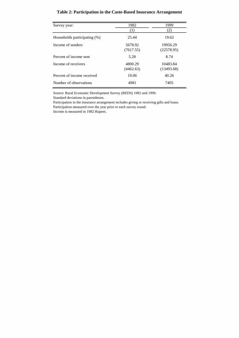
Table 2: Participation in the Caste-Based Insurance Arrangement

Survey year: 1982 1999(1) (2)

Households participating (%) 25.44 19.62

Income of senders 5678.92 19956.29(7617.55) (22578.95)

Percent of income sent 5.28 8.74

Income of receivers 4800.29 10483.84(4462.63) (13493.68)

Percent of income received 19.06 40.26

Number of observations 4981 7405

Source: Rural Economic Development Survey (REDS) 1982 and 1999.Standard deviations in parentheses.Participation in the insurance arrangement includes giving or receiving gifts and loans.Participation measured over the year prior to each survey round.Income is measured in 1982 Rupees.

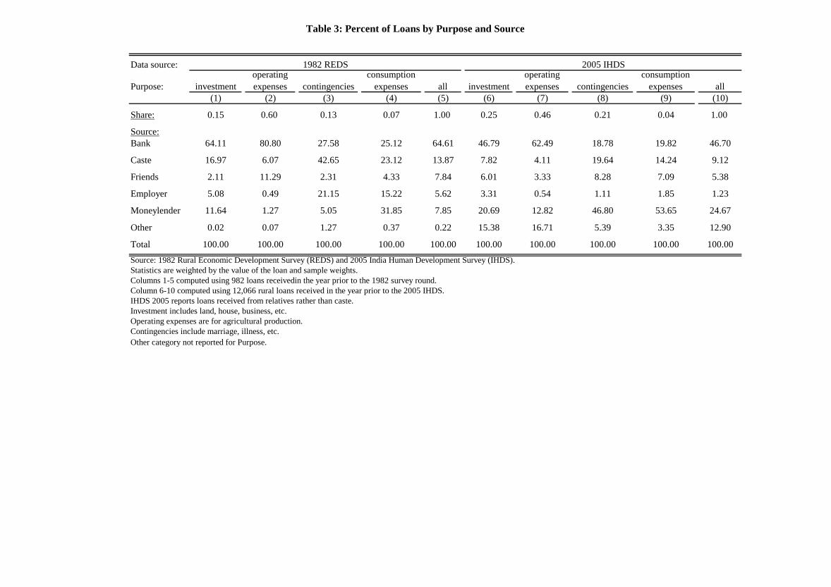
Table 3: Percent of Loans by Purpose and Source

Data source:

Purpose: investmentoperating expenses contingencies

consumption expenses all investment

operating expenses contingencies

consumption expenses all

(1) (2) (3) (4) (5) (6) (7) (8) (9) (10)

Share: 0.15 0.60 0.13 0.07 1.00 0.25 0.46 0.21 0.04 1.00

Source:Bank 64.11 80.80 27.58 25.12 64.61 46.79 62.49 18.78 19.82 46.70

Caste 16.97 6.07 42.65 23.12 13.87 7.82 4.11 19.64 14.24 9.12

Friends 2.11 11.29 2.31 4.33 7.84 6.01 3.33 8.28 7.09 5.38

Employer 5.08 0.49 21.15 15.22 5.62 3.31 0.54 1.11 1.85 1.23

Moneylender 11.64 1.27 5.05 31.85 7.85 20.69 12.82 46.80 53.65 24.67

Other 0.02 0.07 1.27 0.37 0.22 15.38 16.71 5.39 3.35 12.90

Total 100.00 100.00 100.00 100.00 100.00 100.00 100.00 100.00 100.00 100.00

Source: 1982 Rural Economic Development Survey (REDS) and 2005 India Human Development Survey (IHDS).Statistics are weighted by the value of the loan and sample weights.Columns 1-5 computed using 982 loans receivedin the year prior to the 1982 survey round.Column 6-10 computed using 12,066 rural loans received in the year prior to the 2005 IHDS.IHDS 2005 reports loans received from relatives rather than caste.Investment includes land, house, business, etc.Operating expenses are for agricultural production.Contingencies include marriage, illness, etc.Other category not reported for Purpose.

1982 REDS 2005 IHDS

Table 4: Percent of Loans by Type and Source

Data source: 2005 IHDS

Loan type: without interest without collateralwithout collateral

or interest without interest(1) (2) (3) (4)

Source:

Bank 0.57 23.43 0.38 0.00

Caste 28.99 60.27 20.38 44.62

Friends 9.35 91.72 3.89 21.5

Employer 0.44 65.69 0.44 10.75

Moneylender 0.00 98.71 0.00 0.27

Source: 1982 Rural Economic Development Survey (REDS) and 2005 India Human Development Survey (IHDS).Statistics are weighted by the value of the loan and sample weights.Columns 1-3 computed using 982 loans received in the year prior to the 1982 survey round.Column 4 computed using 12,066 rural loans received in the 5 years prior to the 2005 IHDS.IHDS 2005 reports loans received from relatives rather than caste.The reference category is caste loans.

1982 REDS

Table 5: Income and Consumption within the Caste

Data Source: relative income

relative consumption

consumption-income ratio

relative income

relative consumption

consumption-income ratio migration

(1) (2) (3) (4) (5) (6) (7)Relative Income class:

1 0.119 0.460 3.871 0.316 0.843 2.665 0.0322 0.281 0.625 2.224 0.416 0.854 2.052 0.0343 0.373 0.626 1.680 0.513 0.871 1.697 0.0514 0.510 0.673 1.319 0.627 0.887 1.413 0.0465 1.000 1.000 1.000 1.000 1.000 1.000 0.051

Note: Income classes are defined by quintiles within each caste.Income and consumption are measured relative to the highest (fifth) income class.REDS 2006 income and consumption are inputted from ICRISAT data.REDS data consists of 100 castes, while ICRISAT data consist of 7 castes. Sample-size restriction is at least 30 households per caste with REDS data and 20 households per caste with ICRISAT data.

ICRISAT REDS 2006

Table 6: Reduced-Form Migration Estimates

Dependent variable:(1) (2) (3) (4) (5) (6)

Household Income 0.0059 0.0051 0.0026 0.0025 0.0021 0.0021(0.0024) (0.0024) (0.0033) (0.0033) (0.0030) (0.0036)

Caste Income -0.016 -0.018 -0.022 -0.024 -0.025 -0.017(0.0043) (0.0055) (0.008) (0.0107) (0.0107) (0.014)

Income Risk -- -0.00038 -0.00037 -0.00053 -0.00053 -0.00053(0.00015) (0.00016) (0.00017) (0.00017) (0.00011)

Village Income 0.007 0.006 -- --(0.011) (0.013) -- --

Village/ Caste Income 0.0073 0.0088(0.013) (0.028)

Village Fixed Effects No No No No No YesInfrastructure Variables No No No Yes Yes No

Joint sig. of infrastructure variables:χ2 -- -- -- 16.14 16.59 --

-- -- -- [0.0011] [0.00090] --

Number of observations 19,362 19,362 19,362 19,362 19,362 19,362

Source: 2006 Rural Economic Development Survey (REDS) census.Bootstrapped standard errors in parentheses are clustered at the caste level in Columns 1 - 2 and 6 and two-way clustered at the caste and village level in Columns 3 - 5.Income measured in lakhs of Rupees, (1 lakh = 100,000).Infrastructure variables : whether there is a bank, secondary school, health center, or bus station in the village, as well as distance to the nearest town. chi-square p-value reported in square brackets.Sample-size restricted to castes with at least 30 households.

migration

Table 7: Structural Estimates

relative consumption migration

relative consumption migration

relative consumption migration

relative consumption migration

relative consumption migration

(1) (2) (3) (4) (5) (6) (7) (8) (9) (10)Relative Income Class:

1 0.843 0.032 0.801 0.000 0.794 0.000 0.751 0.000 0.730 0.032(0.071) (0.00020) (0.058) (0.00018) (0.097) (0.000081) (0.083) (0.0095)

2 0.854 0.034 0.817 0.014 0.810 0.014 0.767 0.011 0.744 0.032(0.070) (0.0073) (0.059) (0.0075) (0.092) (0.010) (0.064) (0.052)

3 0.871 0.051 0.834 0.039 0.827 0.039 0.792 0.029 0.765 0.046(0.063) (0.0083) (0.053) (0.0088) (0.070) (0.025) (0.055) (0.027)

4 0.887 0.046 0.868 0.060 0.863 0.060 0.842 0.055 0.825 0.044(0.044) (0.0089) (0.038) (0.0095) (0.044) (0.033) (0.037) (0.013)

5 1.000 0.051 1.000 0.100 1.000 0.101 1.000 0.119 1.000 0.051(0.014) (0.019) (0.062) (0.0074)

overall 0.043 0.043 0.043 0.043 0.041β

α

γ

Source: 2006 Rural Economic Development Survey (REDS) census.Structural estimation is based on 100 castes with at least 30 households in the census.Relative income classes are defined by quintiles within each caste. Consumption is measured relative to the highest (fifth) income class in Columns 1, 3, 5, 7, and 9.Relative consumption and migration are computed as the average in each income-class across all castes.Jackknifed standard errors in parentheses.We match on two moments - migration in the lowest and the highest relative income class - in the flexible specification (Columns 9-10).Standard errors for those two income classes in Column 10 thus reflect sampling error due to the jack-knife procedure.β = α + γMak in Columns 9-10. The estimated α and γ parameters are used to compute β for the representative household with mean-wealth in the REDS census.

1.410

(0.050)

(0.91)4.45

(0.92)0.012--

estimating ν by absolute income-classmeasured estimating ν by caste

-- ----

0.991(0.18)

1.218 0.845(0.91)

--

single ν

(0.78)--

Table 8: FE-IV Migration and Out-Marriage Estimates

Data source:Dependent variable: migration out-marriage

(1) (2)

Household income 0.262 0.166(0.147) (0.102)

Caste income -0.110 -0.111(0.053) (0.054)

Time trend 0.059 0.026(0.020) (0.011)

Kleibergen-Paap F-statistic 10.52 8.05

Number of observations 1,049 998

Wild cluster bootstrapped standard errors are clustered at the state level.Income is constructed using wealth- and wage-based measure. Income measured in lakhs of Rupees, (1 lakh = 100,000).Additional regressors: whether anyone in the village used HYV and share of village land irrigated in 1971 (household and caste average). Excluded variables: inherited land, interaction of any HYV and irrigation share, interaction of inherited land, any HYV and irrigation share (household and caste average).

households with heads at least age 18 in 1982.Stock-Yogo weak ID test: 5% critical value 15.72, 10% critical value 9.48.

1982 REDS

Source: Rural Economic Development Survey (REDS) panel, 1982 and 1999.

Sample restricted to castes with at least 10 households in the panel and

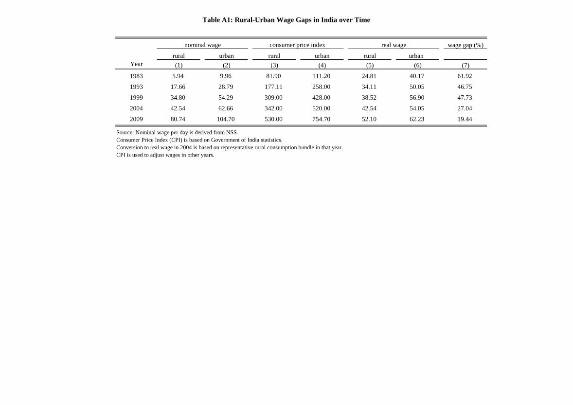
Table A1: Rural-Urban Wage Gaps in India over Time

wage gap (%)

rural urban rural urban rural urban Year (1) (2) (3) (4) (5) (6) (7)

1983 5.94 9.96 81.90 111.20 24.81 40.17 61.92

1993 17.66 28.79 177.11 258.00 34.11 50.05 46.75

1999 34.80 54.29 309.00 428.00 38.52 56.90 47.73

2004 42.54 62.66 342.00 520.00 42.54 54.05 27.04

2009 80.74 104.70 530.00 754.70 52.10 62.23 19.44

Source: Nominal wage per day is derived from NSS.Consumer Price Index (CPI) is based on Government of India statistics.Conversion to real wage in 2004 is based on representative rural consumption bundle in that year. CPI is used to adjust wages in other years.

nominal wage consumer price index real wage

Table A2: Loan Characteristics by Source

Dependent Variable: without interest without collateral

(1) (2)

Bank -0.243 -0.329(0.021) (0.037)

Friends -0.058 0.127(0.041) (0.072)

Employer -0.227 0.009(0.030) (0.052)

Moneylender -0.247 -0.005(0.025) (0.044)

Other 0.075 0.206(0.061) (0.108)

Number of Observations 1045 1045

Note: The other categories are not reported.Observations are weighted by the value of the loan and sample weights.Caste is the omitted source in these regressions.

loan type

Table A3: Household Characteristics, Income-gain, Migration rate and ν parameter by Absolute Income-Classes

household income land value

number of working adults

education of household head

income-gain from migration

migration rate ν parameter

(1) (2) (3) (4) (5) (6) (7)Absolute Income class:

1 0.023 38084.74 1.462 4.684 0.218 0.043 19.609

2 0.040 35956.19 1.451 3.909 0.228 0.010 27.352

3 0.051 114863.00 1.656 3.744 0.179 0.024 28.030

4 0.100 129849.50 1.777 5.083 0.190 0.051 21.576

5 0.894 90414.75 1.950 4.741 0.166 0.026 27.329

Source: 2006 Rural Economic Development Survey (REDS) census.Absolute income classes are defined by quintiles across the entire income distribution, without regard to caste affiliation.Household income based on assets, number of working adults, education (from REDS) and rural, urban wages (from NSS).Income-gain is computed assuming a single member of the household migrates.Migration rate is obtained from the REDS, and together with the income-gain from migration, is used to derive the ν parameter.

Table A4: Structural Estimates with 4 and 6 Relative Income-Classes

Number of relative income-classes:

relative consumption migration

relative consumption migration

relative consumption migration

relative consumption migration

(1) (2) (3) (4) (5) (6) (7) (8)Relative Income class:

1 0.857 0.031 0.817 0.000 0.831 0.033 0.785 0.000(0.059) (0.0008) (0.052) (0.0000)

2 0.880 0.042 0.837 0.022 0.837 0.027 0.797 0.013(0.058) (0.0084) (0.052) (0.0073)

3 0.894 0.048 0.866 0.051 0.854 0.050 0.812 0.025(0.044) (0.0077) (0.049) (0.0106)

4 1.000 0.050 1.000 0.097 0.854 0.047 0.829 0.043(0.0138) (0.045) (0.0110)

5 -- -- -- -- 0.883 0.047 0.867 0.064(0.037) (0.0102)

6 -- -- -- -- 1.000 0.053 1.000 0.113(0.0178)

overall 0.043 0.043 0.043 0.043(0.0060) (0.0063)

β

Source: 2006 Rural Economic Development Survey (REDS) census.Structural estimation is based on 100 castes with at least 30 households in the census.Four and six equal-sized income classes are constructed within each caste. Benchmark specification (single v) in all estimations.Consumption is measured relative to the highest income class in Column 1 and Column 5.Relative consumption and migration are computed as the average in each relative income-class across all castes.Jackknifed standard errors in parentheses.

(0.814)(0.813)1.319 1.487

four six

estimated estimatedmeasured measured

Table A5: First-Stage Estimates

Dependent variable: hh

income change

caste income change

(1) (2)

Anyone in the village used HYV (household) -2787.65 20369.17 (3719.06) (17642.30)

Anyone in the village used HYV (caste average) -3348.87 -42467.91 (4990.63) (39691.53)

Share of village land irrigated (household) -56.24 5578.18 (4063.92) (9886.26)

Share of village land irrigated (caste average) -4094.89 -22929.07 (3144.29) (32659.12)

HYV*irrigation share (household) 1844.46 -26942.14 (5847.23) (22377.58)

HYV*irrigation share (caste average) -1646.46 24413.53 (6428.40) (45272.26)

inherited land (household) 3.48 -5.32 (1.12) (4.55)

inherited land (caste average) 6.48 24.11 (7.88) (43.01)

HYV*irrigation share*inherited land (household) 3.44 6.58 (6.06) (14.78)

HYV*irrigation share*inherited land (caste average) 41.09 140.68

(19.56) (37.31) Constant 8084.81 25683.28

(2828.20) (20544.49) F statistic (excluded variables) 104.96 12.28 p-value 0.00 0.00 R-squared 0.02 0.07 Number of observations 2335 2335 Standard errors in parentheses are robust to clustering at the state level. Dependent variables are computed as the change between 1982 and 1999. Income is constructed using a wealth-based measure. Excluded variables: HYV*irrigation, inherited land, HYV*irrigation*inherited land (household and caste average) Regressions restricted to castes with at least 10 households in sample and households with heads at least age 18 in 1982.

 

 

 

 

 

Table A6: FE-IV Network Participation Estimates

Data source: 1982 REDSDependent variable: network participation

(1)

Household income -0.520(0.684)

Caste income 0.327(0.173)

Time trend 0.014(0.123)

Kleibergen-Paap F-statistic 10.52

Number of observations 1,049

Wild cluster bootstrapped standard errors are clustered at the state level.Income is constructed using wealth- and wage-based measure. Income measured in lakhs of Rupees, (1 lakh = 100,000).Additional regressors: whether anyone in the village used HYV and share of village land irrigated in 1971 (household and caste average). Excluded variables: inherited land, interaction of any HYV and irrigation share, interaction of inherited land, any HYV and irrigation share (household and caste average).

households with heads at least age 18 in 1982.Stock-Yogo weak ID test: 5% critical value 15.72, 10% critical value 9.48.

Source: Rural Economic Development Survey (REDS) panel, 1982 and 1999.

Sample restricted to castes with at least 10 households in the panel and

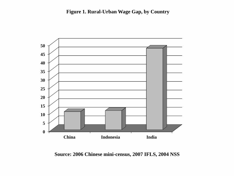
Figure 1. Rural-Urban Wage Gap, by Country

0

5

10

15

20

25

30

35

40

45

50

China Indonesia India

Source: 2006 Chinese mini-census, 2007 IFLS, 2004 NSS

15

20

25

30

35

40

45

50

55

60

65

1983 1993 1999 2004 2009

Figure 2. Real Rural and Urban Wages in India

Source: 1983-2009 NSS

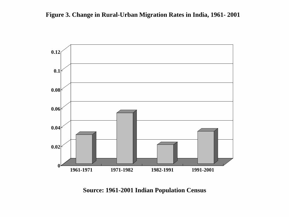
0

0.02

0.04

0.06

0.08

0.1

0.12

1961-1971 1971-1982 1982-1991 1991-2001

Figure 3. Change in Rural-Urban Migration Rates in India, 1961- 2001

Source: 1961-2001 Indian Population Census

0

5

10

15

20

25

30

35

40

45

China Indonesia India Nigeria

1975 2000

Figure 4. Change in Percent Urbanized, by Country, 1975-2000

Source: UNDP 2002

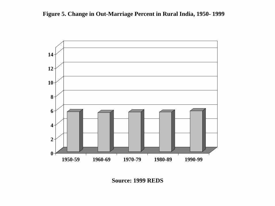
Figure 5. Change in Out-Marriage Percent in Rural India, 1950- 1999

0

2

4

6

8

10

12

14

1950-59 1960-69 1970-79 1980-89 1990-99

Source: 1999 REDS

Figure 6. Counter-Factual Simulation

0

0.03

0.06

0.09

0.12

0.15

0.18

0.21

0 10 20 30 40 50 60 70 80 90

Pred

icte

d M

igra

tion

Percent Change in β and ν

flexiblebenchmark

β

ν

Figure 7. Reducing Risk in Higher Income-classes

0.45

0.50

0.55

0.60

0.65

0.70

0.75

0.00

0.05

0.10

0.15

0.20

0.25

0.30

0 10 20 30 40 50 60 70 80 90

Pred

icte

d L

ambd

a

Pred

icte

d M

igra

tion

Percent Decrease in Beta (third, fourth and fifth absolute income-classes)

lambda (lowest class)

migration (highest class)

migration (lowest class)

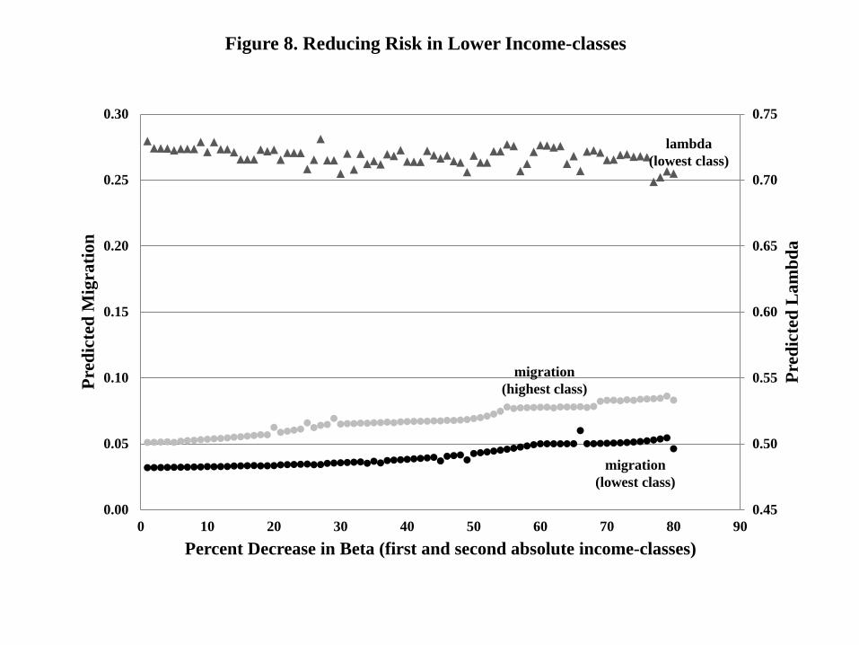
Figure 8. Reducing Risk in Lower Income-classes

0.45

0.50

0.55

0.60

0.65

0.70

0.75

0.00

0.05

0.10

0.15

0.20

0.25

0.30

0 10 20 30 40 50 60 70 80 90

Pred

icte

d L

ambd

a

Pred

icte

d M

igra

tion

Percent Decrease in Beta (first and second absolute income-classes)

lambda (lowest class)

migration (highest class)

migration (lowest class)

0.03

0.04

0.05

0.06

0.07

0.08

0.09

0.1

0 5 10 15 20 25 30 35 40 45 50

Pred

icte

d M

igra

tion

Percent decrease in ν

beta = .705

beta = 1.41

Figure A1. Counter-Factual Simulations