Financing Intermediate Inputs and Misallocation:

Evidence from China’s Firm-Level Data

Wenya Wang∗

August 12, 2020

Abstract

This paper finds the misallocation of intermediate inputs in China’s firm-level

data, eliminating which increases the average industry’s gross output by 4.98%. Ev-

idences of pre-pay frictions and borrowing constraints on intermediates are found. I

build these frictions into a standard firm investment model with adjustment costs and

borrowing constraints on capital. Counterfactuals show that the borrowing constraint

on intermediates and on capital each accounts for 23% of China’s gross output mis-

allocation. Value-added gains from reallocating capital, labor and intermediates are

smaller than those using the Hsieh and Klenow (2009)’s approach, both in the model

and in the data.

JEL Codes: E44, G31, G32, L60, O33, O47

Key Words: Misallocation, Intermediate Inputs, Pre-pay, Borrowing Constraints

∗School of Finance, Shanghai University of Finance and Economics, 322 Tongde Building, 100 Wudong

Road, Shanghai, 200433, P.R. China (email: wang.wenya@mail.shufe.edu.cn). I am greatly indebted to my

supervisor Jim MacGee for his intellectual coaching, mentoring, and support. I deeply thank Igor Livshits,

David Rivers, Simona Cociuba, Xiaodong Zhu, Loren Brandt, Michael Song, Johannes Van Biesebroeck,

and Sophie Osotimehin for their insightful discussions. I thank conference participants in NAESM (Davis),

SAET (Taipei), Wuhan University CERW Workshop, Midwest Macro Workshop (LSU), and AESM (Hong

Kong). Lastly, I thank SUFE finance fin-lab for their assistance in computation. All errors are mine.

1

Operating a firm involves purchases and payments for intermediate inputs, the rev-

enue share of which exceeds 50% (Jones, 2011). In many countries, firms finance these

payments for several months due to time-consuming production processes and late sales

payments. A strand of the corporate finance literature discusses how to optimize working

capital to cover these payments (e.g., Jose, Lancaster, and Stevens, 1996; Deloof, 2003).

Although intermediate inputs are a crucial input for production, little on its misal-

location has been discussed. In their seminal work, Hsieh and Klenow (2009) find that

marginal revenue products of capital and labor are dispersed across firms within finely

defined industries in China, India, and the United States. The potential aggregate out-

put gain if these dispersions were removed is quantified as misallocation, suggesting the

existence of frictions or policy distortions. Follow-up studies further investigate the spe-

cific frictions and distortions primarily on the inputs of capital and labor, but rarely on

intermediate inputs.1

This paper studies the intermediate input misallocation. Using the Chinese Above-

Scale Industrial Enterprise Survey (AIES) dataset 1998-2007, the paper first finds that in-

termediate inputs are misallocated. If marginal revenue products of intermediate inputs

(MRPM) were equalized across firms alone, an average 2-digit Chinese Industrial Clas-

sification (CIC) industry would increase its gross output by 4.98% and value-added by

20.61%. The magnitudes are close to the gains obtained by reallocating capital alone.

I then find evidence of two frictions on intermediate inputs in the data, i.e., pre-pay

and borrowing constraints. Like in other countries, an average 70-day window exists be-

tween firms’ expenditures on intermediates and the recovery of sales receipts in China.

With this pre-pay friction, financial frictions could hinder firms from choosing the op-

timal amount of intermediate inputs, and induce a dispersion in its marginal revenue

products. I identify the financial friction by looking at whether financial development

across Chinese provinces decreases the misallocation measure, i.e., the coefficient of vari-

1One exception is Boehm and Oberfield (2018). There are studies that explicitly model intermediate

inputs as the third factor in productions, e.g., Jones (2011), Bils, Klenow, and Ruane (2017) and Baqaee and

Farhi (2020). But few studies consider explicitly whether intermediates are misallocated in the data and

what causes there are.

2

ation in MRPM, more for financially vulnerable industries (Rajan and Zingales, 1998;

Braun, 2003). Results suggest that a one standard deviation increase in financial develop-

ment decreases the coefficient of variation by 33 percent of its standard deviation across

industries and provinces. Additional decreases by 6 and 2 percent are identified if the

industry is one standard deviation lower than average in asset tangibilities and higher in

external financial dependences, respectively.

How could the intermediate input frictions interact with capital frictions that are bet-

ter understood in the literature (e.g., Bartlesman, Haltiwanger, and Scarpetta, 2013; Asker,

Collard-Wexler, and De Loecker, 2014; Midrigan and Xu, 2014)? Does a model with inter-

mediate input frictions quantitatively account more for the misallocation in China’s man-

ufacturing sector? To answer these questions, I build the intermediate good frictions into

a standard partial equilibrium model of firm investment a la Cooper and Haltiwanger

(2006), along with capital frictions of borrowing constraints and adjustment costs. The

model is for a representative industry. Firms produce differentiated products that ag-

gregate into a CES industry-level bundle. They maximize net present values of future

dividends given stochastic productivities and an option to exit and default every period.

Intermediate inputs are determined, and a fraction of the cost needs to be pre-paid a pe-

riod ahead, which increases firms’ financing needs in addition to capital expenditures.

Competitive intermediaries provide the financings and charge an interest rate that de-

pends on the default probability.

To quantify how much the model can account for the measured misallocation in the

data, I calibrate the model to match key moments in AIES. Reallocation exercises in the

model simulated data suggest that the benchmark model well captures the AIES data

in the magnitude of misallocations. In the model simulated sample of AIES analog, the

gross output would increase by 5.37% and value-added by 13.97%, if only marginal rev-

enue products of intermediate inputs were equalized. These numbers are comparable to

those aforementioned for an average 2-digit industry in AIES. Meanwhile, if marginal

products of capital, labor, and intermediate inputs were all equalized, the gross output

would increase by 21.84%, and value-added by 58.87%. This paper calls the percentage of

potential gross output gains as the gross output misallocation and value-added gains as

3

the value-added misallocation. Hence, the model accounts for 100% of the gross output

misallocation and 65% of the value-added misallocation in AIES.

Further counterfactuals remove subsets of frictions to quantify the misallocation ac-

counted by each friction. In a model with only the one-period time-to-build capital

friction, the gross output misallocation is 13.11%, and the value-added misallocation

is 43.69%. The dynamic nature of capital with stochastic firm-level productivities con-

tributes the most misallocation, consistent with Asker et al. (2014). Intermediate input

and capital frictions account for about half-half of the difference in misallocations be-

tween the benchmark model and the model with only the one-period time-to-build fric-

tion on capital. The pre-pay and borrowing constraints on intermediate inputs, mostly

the latter, account for 62% of the remaining gross output misallocation. This number is

52% for the capital frictions, mostly from the borrowing constraints on capital. This pa-

per hence contributes to the discussion on financial frictions and misallocation (e.g., Buera

and Shin, 2013; Midrigan and Xu, 2014; Moll, 2014), and argues that the effect of financial

frictions on misallocation doubles when it distorts both capital and intermediate inputs.

The output gains from reallocation exercises throughout the paper are first defined

as changes in gross output and then in value-added. This differs from the conventional

value-added approach (Hsieh and Klenow, 2009) that subtracts intermediate inputs from

the gross output, and models firms as value-added producers. How do the two ap-

proaches differ given the same firm-level dataset? With an elasticity of substitution vary-

ing from 3 to 7, I find that the value-added approach gives a value-added misallocation

2 to 3 times as large as that obtained under the gross output approach, both in the model

and in the data. Further algebra shows that intermediate distortions, if there is any, could

amplify dispersions of returns to capital when one mistakenly models firms as value-

added producers. With a multiplicative increase of capital share in the value-added pro-

duction function, this channel substantially increases misallocations. Combined with my

finding of counterfactual experiments, the result suggests that the gap could be narrowed

between the empirically sizable misallocation and the moderate misallocation in dynamic

models of financial frictions previously found in the literature.

This paper first contributes to studies that follow a direct approach and investigate

4

what frictions and distortions could rationalize the misallocation in firm-level datasets for

many countries, pioneered by Hsieh and Klenow (2009).2 One extensively studied theme

is capital misallocation and its causes.3 Some argue the importance of dynamic capi-

tal and its adjustment costs (Bartlesman et al., 2013; Asker et al., 2014). Others focus on

financial frictions, by which the misallocation could be moderate when firms can accumu-

late net worth and self-finance. This self-financing channel does not undo misallocation

when productivities are less persistent (Caselli and Gennaioli, 2013), when there are fixed

cost barriers (Midrigan and Xu, 2014) , when the initial state of the economy is badly mis-

allocated (Buera and Shin, 2013) and when borrowing constraints are endogenous and

size-dependent (Gopinath, Kalemli-Ozcan, Karabarbounis, and Villegas-Sanchez, 2017;

Bai, Lu, and Tian, 2018). This paper shows another possibility that financial constraints

bind more if there are recurrent financing needs for intermediate inputs.

This paper also contributes to the work that links intermediate inputs to the TFP.

Works include an input-output amplifier of distortions via intermediate inputs (Jones,

2011; Bartelme and Gorodnichenko, 2015; Osotimehin and Popov, 2020), working capital

constraints on intermediate inputs and the TFP in crisis of emerging economies (Mendoza

and Yue, 2012; Pratap and Urrutia, 2012), and legal enforcement frictions on intermediate

inputs transactions (Boehm and Oberfield, 2018). This paper complements these studies

by applying working capital constraints of intermediate inputs onto the discussions of

misallocation.

This paper is lastly but not leastly related to a large literature on misallocation in

China. Hsieh and Klenow (2009) first find substantial misallocation in Chinese data.

Brandt, Van Biesebroeck, and Zhang (2012) further document a limited input realloca-

tion across firms in China despite of its high TFP growth over 1998-2007. Explanations

for misallocation include preferred lendings to the state-owned firms (Song, Storesletten,

2See Restuccia and Rogerson (2013), Hopenhayn (2014) and Buera, Kaboski, and Shin (2015), for a com-

prehensive review.3Other explanations include information frictions (David, Hopenhayn, and Venkateswaran, 2016; David

and Venkateswaran, 2019), heterogeneous and non-isoelastic production functions (Haltiwanger, Kulick,

and Syverson, 2018; Uras and Wang, 2018), heterogeneous markups (Peters, 2013; Baqaee and Farhi, 2020)

and housing bubbles (Miao and Wang, 2014), to name a few.

5

and Zilibotti, 2011; Brandt, Tombe, and Zhu, 2013), trade and migration costs (Tombe

and Zhu, 2019), entry costs (Brandt, Kambourov, and Storesletten, 2018), and financial

frictions (Bai et al., 2018), to name a few examples.

The rest of this paper is structured as follows. Section 1 illustrates the distortions in

intermediate inputs allocation in AIES, and introduces frictions of pre-pay and borrow-

ing constraints. Section 2 presents the model. Section 3 calibrates the model, computes

the misallocation in the model and in the data, implements decomposition exercises of

misallocation contributed by each friction, and discusses economic mechanisms. Section

4 concludes.

1 Intermediate Input Misallocation in Data

This section first describes China’s firm-level data, in which I document intermediate

input misallocation of a magnitude comparable to capital misallocation. I then show sug-

gestive evidence of pre-pay frictions and borrowing constraints on intermediate inputs.

1.1 Data

This paper uses Chinese Above-scale Industrial Enterprise Survey (AIES) data collected

by the National Bureau of Statistics (NBS) from 1998 to 2007. The dataset has been exten-

sively studied (see, e.g., Hsieh and Klenow, 2009; Brandt, Van Biesebroeck, and Zhang,

2014; Bai et al., 2018; David and Venkateswaran, 2019). The unit of observation in the

data is a firm with unique registration IDs at the State Administration for Industry and

Commerce (SAIC). The dataset combines annual firm-level balance sheets, income, and

cash flow statements for all state-owned manufacturing firms and non-state-owned ones

with sales above 5 million yuan before 2007.4 During this period, the number of firms in

the data increased from 147,690 in 1998 to 304,599 in 2007.

Variables of interest include gross output, book value of capital, employment, wage

bill, intermediate input cost, opening year, inventory, account payables and receivables,

4The sales threshold became also applicable for state-owned firms starting from 2007. In 2011, the thresh-

old increased to 20 million yuan.

6

interest expense, total liability, ownership, and industries. Industries are classified by the

1994 version of the 4-digit China Industrial Classification (CIC) codes before 2002 and the

2003 version after. Concordances of the two versions are done at the broader 2-digit CIC

levels. Further, the original data are cross-sectional each year, and I match firms over the

years to construct a 10-year unbalanced panel. Nominal values of output and inputs in the

unbalanced panel are deflated to constant 1998 yuan using the industry-level deflators.5

1.2 Misallocation of Intermediate Inputs

This subsection presents evidence of the intermediate input misallocation in China’s data.

I start describing the conceptual framework similar to that of Hsieh and Klenow (2009), in

which firms are now modeled as gross output producers. Aggregate output Y is produced

by a Cobb-Douglas production function of output from each industry

Y = ΠSs=1Yθs

s (1)

where θs represents the expenditure share of industry s, and ∑Ss=1 θs = 1. Y is used for

household final consumption C and as the intermediate input in further productions M,

i.e., Y = C + M.

Output of industry s, Ys, is produced under monopolistic competitions with an elas-

ticity of substitution σ

Ys = (Ns

∑is

Yσ−1

σis )

σσ−1 (2)

Firm i in industry s produces gross output quantity

Yis = exp(zis)Kαs

kis L

αsl

is M1−αs

k−αsl

is (3)

and revenue

PisYis = PsY1σ

s exp(zis)σ−1

σ Kαs

kis L

αsl

is Mαsm

is

= exp(zis)Kαs

kis L

αsl

is Mαsm

is (4)

5Codes used for matching and industry-level deflators are borrowed from Brandt et al. (2012). See

Appendix for details about how I match firms over the years.

7

where zis is log quantity productivity, and zis is log revenue productivity.6 Here I define

zis = logPsY1σ

s + zis. Kis, Lis and Mis denote firm-level capital, labor and intermediate

inputs. Note that the industry-specific revenue and cost shares are related, i.e., αsk =

αsk

σ−1σ , αs

l = αsl

σ−1σ , and αs

m = (1− αsk − αs

l )σ−1

σ .

Firms face distortions τyis in output, τm

is in intermediate inputs, τlis in labor and τk

is in

capital, i.e.,

MRPKis := αsk

PisYis

Kis=

1 + τkis

1− τyis

R (5)

MRPLis := αslPisYis

Lis=

1 + τlis

1− τyis

w (6)

MRPMis := (1− αsk − αs

l )PisYis

Mis=

1 + τmis

1− τyis

P (7)

where Pis is firm i’s output price in industry s, w and R are labor and capital rental prices.

Intermediate input price is P, which is also the price for aggregate output. I use sales for

PisYis, wage payment for effective units of labor Lis, capital stock for Kis, and intermediate

input for Mis in constant 1998 yuan to compute these marginal products.7 As in most

firm-level datasets, AIES does not report prices and quantities of output and inputs.

My benchmark procedure trims the top and the bottom 1% of TFPR and TFPQ distri-

butions across industries for each year. I set αsm and αs

l , as the median intermediate inputs

and labor shares within 2-digit industries in the data. Capital shares are set as 0.85 mi-

6I slightly abuse the language here, since log revenue productivity, TFPR, is defined as

TFPRis = log(PisYis)− αsl log(Lis)− αs

klog(Kis)− (1− αsk − αs

l )log(Mis)

which is a linear transformation of zis plus an industry-level constant. Note that log quantity productivity,

TFPQ, is

TFPQis = log(Yis)− αsl log(Lis)− αs

klog(Kis)− (1− αsk − αs

l )log(Mis)

7Capital stock is constructed using a perpetual inventory method, setting the initial year as 1995. For

more discussions, see Brandt et al. (2012).

8

nus the sum of intermediate input and labor shares, implying an elasticity of substitution

σ = 6.67.8

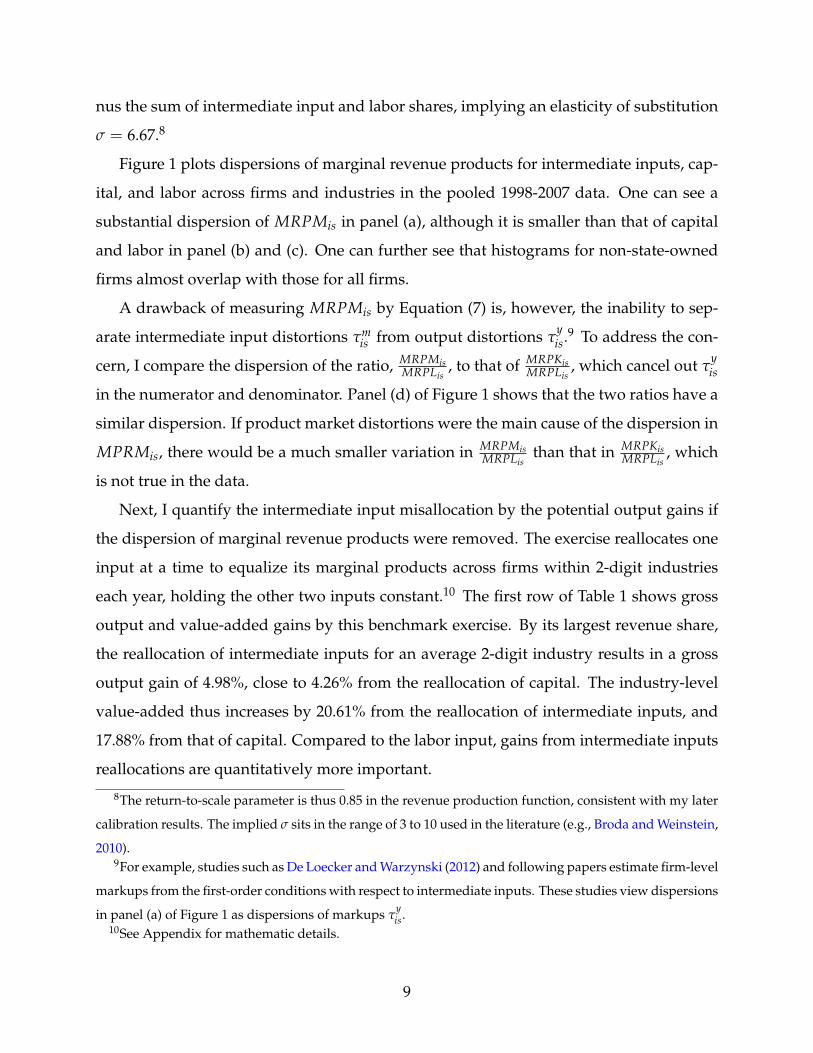
Figure 1 plots dispersions of marginal revenue products for intermediate inputs, cap-

ital, and labor across firms and industries in the pooled 1998-2007 data. One can see a

substantial dispersion of MRPMis in panel (a), although it is smaller than that of capital

and labor in panel (b) and (c). One can further see that histograms for non-state-owned

firms almost overlap with those for all firms.

A drawback of measuring MRPMis by Equation (7) is, however, the inability to sep-

arate intermediate input distortions τmis from output distortions τ

yis.

9 To address the con-

cern, I compare the dispersion of the ratio, MRPMisMRPLis

, to that of MRPKisMRPLis

, which cancel out τyis

in the numerator and denominator. Panel (d) of Figure 1 shows that the two ratios have a

similar dispersion. If product market distortions were the main cause of the dispersion in

MPRMis, there would be a much smaller variation in MRPMisMRPLis

than that in MRPKisMRPLis

, which

is not true in the data.

Next, I quantify the intermediate input misallocation by the potential output gains if

the dispersion of marginal revenue products were removed. The exercise reallocates one

input at a time to equalize its marginal products across firms within 2-digit industries

each year, holding the other two inputs constant.10 The first row of Table 1 shows gross

output and value-added gains by this benchmark exercise. By its largest revenue share,

the reallocation of intermediate inputs for an average 2-digit industry results in a gross

output gain of 4.98%, close to 4.26% from the reallocation of capital. The industry-level

value-added thus increases by 20.61% from the reallocation of intermediate inputs, and

17.88% from that of capital. Compared to the labor input, gains from intermediate inputs

reallocations are quantitatively more important.

8The return-to-scale parameter is thus 0.85 in the revenue production function, consistent with my later

calibration results. The implied σ sits in the range of 3 to 10 used in the literature (e.g., Broda and Weinstein,

2010).9For example, studies such as De Loecker and Warzynski (2012) and following papers estimate firm-level

markups from the first-order conditions with respect to intermediate inputs. These studies view dispersions

in panel (a) of Figure 1 as dispersions of markups τyis.

10See Appendix for mathematic details.

9

Figure 1: Marginal Products Histograms, 1998-2007 Pooled Data

(a) Intermediate inputs

Median=1.00

0.0

5.1

.15

Fra

ctio

n

0 1 2 3 4Marginal Product of Intermediate Goods

All Firms Private Owned Firms

(b) Capital

Median=0.23

0.1

.2.3

.4.5

Fra

ctio

n0 5 10

Marginal Product of Capital

All Firms Private Owned Firms

(c) Labor

Median=0.96

0.0

5.1

.15

Fra

ctio

n

0 5 10 15Marginal Product of Labor

All Firms Private Owned Firms

(d) Intermediate inputs vs capital

0.0

2.0

4.0

6.0

8F

ract

ion

-4 -2 0 2 4Log relative distortion (to labor)

Intermediate goods Capital

Notes: In panel (a), (b) and (c), solid and hallowed bars plot histograms for marginal revenue products

for all firms and non-state-owned (i.e., non-state-owned) firms in 1998-2007 pooled data. Panel (d) plots

the ratios of marginal revenue products, MRPMisMRPLis

(solid) and MRPKisMRPLis

(hallowed), for all firms in 1998-2007

pooled data.

10

Several alternative procedures are done to test the robustness of results. Procedure

Private keeps only non-state-owned firms for each year. Procedure 4-digit Industry reallo-

cates each input within 4-digit CIC industries. Procedure Trim 2.5 trims the top and the

bottom 2.5% of TFPR and TFPQ distributions. Procedure U.S. Shares uses the industry-

level intermediate input and labor shares from the U.S. NBER-CES productivity database.

The next procedure GE considers the general equilibrium effect triggered by the in-

termediate inputs reallocation. After the reallocation, gross output for each industry in-

creases, which expands the supply of intermediate inputs as a CES bundle of outputs

from all industries. A lower price of intermediate inputs follows, as well as a higher

equilibrium quantity. I approach this idea by setting the revenue shares of intermedi-

ate inputs before and after the reallocation unchanged at the aggregate level, implied by

the Cobb-Douglas production function.11 Numerically, it is to find λ > 1 such that the

reallocation of λ-fold of total intermediate inputs results in an unchanged aggregate in-

termediate input revenue share.

Lastly, the procedure Example Industries checks if the unobserved heterogeneity in in-

termediate input composition, quantity, and price is the main cause for the measured

misallocation. I focus on several industries with the following features: (i) arguably a

Leontif combination of different intermediate inputs; (ii) a homogeneous manufacturing

process across firms; (iii) competitive and standard, not relation-specific, upstream inputs

(Rauch, 1999; Boehm and Oberfield, 2018). These industries are ice making (industry code

1495), cement (industry code 3111), and flat glass (industry code 3141). 12

The rest of Table 1 presents results under the alternative procedures. One could see

that the misallocation of intermediates is robust and not mainly driven by (i) the existence

11 A more rigorous investigation requires a general equilibrium framework that considers the structure

of input-output (Jones, 2011), as well as household labor and saving decisions that affect aggregate labor

and capital. See studies of Bartelme and Gorodnichenko (2015) and Hang, Krishna, and Tang (2019) along

this line.12Table A1 in the appendix also chooses a set of industries with homogeneous output, i.e., arguably

τyis = 0, as in Foster, Haltiwanger, and Syverson (2008) to illustrate similar magnitudes of intermediate input

misallocation. These industries are corrugated & solid fiber boxes, carbon black, ready mixed concrete,

plywood, and sugar.

11

Table 1: Output Gains by Reallocating One Input, 1998-2007 Average

Gross output gains Value-added gains

Procedure Intermediates Capital Labor Intermediates Capital Labor

Benchmark 4.98% 4.26% 2.69% 20.61% 17.88% 11.28%

Private 4.20% 3.49% 2.42% 17.35% 14.63% 10.06%

4-digit Industry 4.50% 3.67% 2.35% 18.64% 15.40% 9.84%

Trim 2.5 3.74% 3.81% 2.57% 16.02% 16.54% 11.14%

U.S. Shares 2.68% 9.22% 7.88% 10.94% 37.91% 32.30%

GE 15.38% 4.26% 2.69% 17.49% 17.88% 11.28%

Example Industries:

1.Ice making (before 2002) 29.58% 9.67% 5.22% 106.66% 34.77% 19.81%

2.Cement 2.32% 5.46% 2.12% 7.60% 17.50% 6.13%

3.Flat glass 3.28% 1.92% 1.17% 17.87% 10.97% 6.26%

Notes: For the Benchmark case, top and bottom 1% of TFPR and TFPQ are trimmed across industries each

year. Reallocation gains are calculated each year at 2-digit industry levels weighted by industry-level gross

output shares. Results above report the averages over 1998-2007.

of state-owned firms; (ii) the potentially overestimated intermediate input share in China;

(iii) heterogeneity in intermediate input compositions, quantities and prices. The level of

misallocation is also higher in terms of gross output, and roughly unchanged in terms of

value-added, if the general equilibrium effect is included.

1.3 Intermediate Input Frictions

Next I aim to provide evidence on pre-pay frictions and borrowing constraints of inter-

mediate inputs to account for its measured misallocation.

Pre-pay Using the value-added output measure, the misallocation literature implicitly

assumes that intermediate inputs are (i) statically chosen and not subject to frictions and

distortions; or (ii) perfectly substitutable with the value-added bundle of capital and labor

at the firm-level. There has been many discussions that intermediate inputs are imperfect

substitutes with the value-added (e.g., Oberfield and Raval, 2014; Ackerberg, Caves, and

Frazer, 2015; Gandhi, Navarro, and Rivers, 2017). Nevertheless, the concept of pre-pay is

12

less discussed, and more emphasized in the trade finance literature. Studies (e.g., Ramey,

1989; Petersen and Rajan, 1997; Antras and Foley, 2015) suggest that a time window ex-

ists between firms’ spending of intermediate inputs purchase and their collection of sales

revenue.

This time window is embodied in the notion of cash conversion cycle (CCC)

CCCis := (Account Receivablesis

Salesis+

InventoryisCOGSis

−Account Payablesis

COGSis)× 365 (8)

for firm i in industry s where COGS is cost of goods, i.e., the sum of intermediate input

costs and wage of production workers. Conceptually, the measure quantifies ”the net time

interval between actual cash expenditures on a firm’s purchase of productive resources

and the ultimate recovery of cash receipts from product sales” (Richards and Laughlin,

1980).

Table 2 reports firm-level summary statistics of CCC and its components of days on in-

ventory (DI), days on receivables (DR), and days on payables (DP). On average, firms in

AIES receive the cash inflow of sales revenue 70 days, i.e., slightly more than two months,

after their cash outflow for intermediate inputs. They hold 71 days of both inventory and

deferred payments from their customers, and 56 days deferral of payments to their sup-

pliers. Although there are firms that have a negative CCC, about 90% of them report a

positive number.13

There is a considerable variation of these measures across firms. The scale of standard

deviations in Table 2 suggests that firms differ in converting cash expenditures to cash ac-

cruals.14 Nevertheless, the heterogeneity and its determinants go beyond the scope of this

13A different notion is operating cycles (OC), i.e., the sum of inventory and receivables divided by sales

standardized by 365 days. The average OC in AIES is 160 days, more than two times of CCC. Thanks to the

suggestions of two anonymous referees, I use CCC instead of OC for the coherency with the model section,

which abstracts the inter-firm trade credit relationships away.14The pattern is more pronounced when one compares the AIES data to Chinese publicly listed firms, the

U.S. Compustat firms and Survey of Small Business Finance (SSBF) firms. For listed firms in China, both

average CCC and DI are longer, about 116 days, and 88 days during the same period. The same pattern

of longer cycles for large and listed firms could also be found in the United States. These facts may reflect

firms’ heterogeneous working capital management abilities (Deloof, 2003), or merely different firm sizes

and positions in supply chains(Cunat, 2007).

13

Table 2: Firm-Level Statistics on Cash Conversion Cycles in AIES Data (Days)

CCC DI DR DP

Mean 70 71 71 -56

SD 101 88 87 68

Notes: DI, DR and DP are days on inventory, receivables and payables. Statistics of DI and DR are from

pooled 1998-2007 data. Statistics of CCC and DP are from pooled 2004-2007 data since AIES does not report

firm-level payables before 2004. Top and bottom 1% of each statistic are trimmed.

paper. I thus follow the literature and describe it as part of the production technologies,

and constant across firms within industries (e.g., Raddatz, 2003; Tong and Wei, 2011), in

order to understand its first-order effect on misallocation.

Financial Frictions With the pre-pay friction, firms could be financially constrained

in intermediate inputs when seeking external financings.15 The constraint is arguably

tighter for firms in financially vulnerable industries ceteris paribus. Thus these industries

may feature higher dispersions in marginal revenue products of intermediate inputs.

To identify the financial friction, I exploit China’s provincial differences in the financial

market development. I investigate whether there would be a larger drop of intermediate

input misallocation for more vulnerable industries than less vulnerable ones, if the indus-

try was in a financially more developed province.16 The identification strategy is similar

to studies such as Raddatz (2003), Tong and Wei (2011) and Manova (2013) that exploit

cross-country variations in financial developments.

I use two proxies to represent financial developments across Chinese provinces, FinDevppt.

One is provincial fractions of loans lent to non-state-owned firms, LoanMktpt, and the

other is the average of LoanMktpt and provincial fractions of deposits held by non-state-

15The same argument applies to the labor input. Focusing on intermediate inputs, rather than labor, is

motivated by its substantially larger share in productions.16A more intuitive illustration of financial frictions is Figure A2 that plots measures of intermediate mis-

allocation against financial vulnerable indexes of industries.

14

owned banks, FinMktpt.17 Both measures are from the NERI Indexes of Marketization

of Chinese Provinces, published by the National Economic Research Institute, China Re-

form Foundation.18 I prefer these indexes over private credit to GDP ratios, since the

latter may represent an inefficient allocation of credit across provinces rather than the

quality of provincial financial markets. For example, during this time period, Beijing had

the highest loan-to-GDP ratio (195%) but ranked only 24th in the LoanMkt index and 15th

in the FinMkt index among 29 provincial regions with non-missing values.

The identification works via the following regression across industry-province obser-

vations:

CV(MRPMspt) = β0 + β1FinDevppt + β2FinDevppt × AssetTangs + β3FinDeppt × ExtFins+

β4FinDeppt × CCCs + β4SOESharespt + β5ExporterSharespt +2007

∑t=1998

δt + ∑p

δp+

∑s

δs + εspt (9)

where s and p are subscripts for 2-digit industries and provinces, respectively. For each

industry, AssetTangs, ExtFins and CCCs are asset tangibilities, external finance depen-

dences and cash conversion cycles that are from the Compustat data. Since firm owner-

ships and exporter statuses may influence misallocation in China’s context, I also control

for fractions of state-owned firms, SOESharest, and exporter firms, ExporterSharespt, for

each industry-province cell. δt, δp and δs are time, province and industry fixed effects.

The dependent variable, the dispersion measure in marginal revenue products of in-

termediate inputs, is its coefficient of variation (CV) at industry-province level, CV(MRPMspt).

Before calculating CVs, I trim the top and bottom 1% of MRPMist for each industry each

year. The key explanatory variables are FinDevppt, and its interactions with AssetTangs

17Non-state-owned banks include joint-equity, city commercial banks, township and village banks, and

agricultural cooperatives. They constituted 30% of total assets and outstanding loans, and 27% of deposits

of the whole banking sector by the end of 2007.18The foundation is supervised by the National Development and Reform Commission (fagaiwei). The

NERI indexes were initially compiled in 1997, with an update every three years. It covers five aspects of

marketizations of provincial economies: relations between the government and markets, developments of

the non-state-owned economies, product markets, factor markets, legal and accounting service markets.

15

and ExtFins. If financial frictions are empirically important, one should expect that finan-

cially vulnerable industries benefit disproportionately more from the provincial financial

market development.

Table 3 presents regression results of which standard errors are clustered within each

industry-province cell. I drop cells that have fewer than 20 firms to avoid small sample

biases. Columns (1) to (6) use the LoanMkt index as the proxy for provincial financial

development levels, while columns (7) to (12) use the FinMkt index. Given the devel-

opment index, the first five columns use the CV(MRPMspt) as the dependent variable,

and the 6th column uses the CV(MRPKspt) as a comparison. Overall, the table shows

that financial market development decreases misallocations of intermediate inputs and

of capital, especially for financially vulnerable industries. For instance, if the financial

development index increases by 1 S.D. in column (1), CV(MRPMspt) decreases by 0.039

for an average industry, and by 0.007 additionally if the industry has an asset tangibility

measure 1 S.D. lower than the average. Similarly, for an industry that has external finance

dependence 1 S.D. higher than the average, there is a further drop in CV(MRPMspt) by

0.002.19 These numbers are fairly stable across specifications except for column (4) and

(10), and the effect via the asset tangibility measure is statistically more significant.

Is the result economically significant? If one looks at statistics of CV(MRPMspt) across

industry-province cells, it averages 0.2354 with a standard deviation of 0.1182. Hence,

when the financial market index, e.g., LoanMkt, increases by 1 S.D. in column (1), the

decrease of intermediate inputs misallocation coming from this channel is about 33 per-

cent of the standard deviation of CV(MRPMspt). This number is 39 percent for industries

with 1 S.D. asset tangibility lower and statistically significant. These results suggest that

financial frictions play a role in inducing intermediate input misallocation.

19Consider the 1 S.D. increase of financial development index, LoanMkt, as relocating an industry from

Tibet to Fujian province. Further, consider the 1 S.D. tangibility decrease as shifting from industry 31 non-

metal mineral products to industry 23 printing and publishing, and 1 S.D. external finance dependence increase

as shifting from industry 17 manufacture of textiles to industry 39 electronic equipment and machinery.

16

Tabl

e3:

Effe

cts

ofPr

ovin

cial

Fina

ncia

lDev

elop

men

ton

Mis

allo

cati

onfo

rIn

dust

ries

wit

hD

iffer

entF

inan

cial

Vul

nera

bilit

ies,

Indu

stry

-Pro

vinc

eC

lust

ered

FinD

evp=

Loan

Mkt

FinD

evp=

Fin

Mkt

CV

(MR

PM)

CV

(MR

PK)

CV

(MR

PM)

CV

(MR

PK)

(1)

(2)

(3)

(4)

(5)

(6)

(7)

(8)

(9)

(10)

(11)

(12)

FinD

evp p

t-0

.012

0**

-0.0

117*

*-0

.013

1**

-0.0

012

-0.0

103

-0.0

276

-0.0

130*

-0.0

130*

-0.0

134*

0.00

18-0

.011

7-0

.013

3

(0.0

040)

(0.0

048)

(0.0

029)

(0.6

357)

(0.0

504)

(0.1

511)

(0.0

113)

(0.0

117)

(0.0

118)

(0.5

882)

(0.0

657)

(0.6

553)

FinD

evp p

t×

Ass

etTa

ngs

0.01

76**

0.01

72**

0.01

24-0

.000

50.

0154

*0.

0520

0.01

82**

0.01

80**

0.01

65*

-0.0

067

0.01

610.

0385

(0.0

015)

(0.0

019)

(0.0

513)

(0.8

783)

(0.0

234)

(0.0

660)

(0.0

087)

(0.0

091)

(0.0

362)

(0.1

305)

(0.0

546)

(0.3

735)

FinD

evp p

t×

Ext

Dep

s-0

.002

4-0

.002

2-0

.002

6-0

.003

4*-0

.002

3-0

.019

2*-0

.003

2-0

.003

1-0

.003

3-0

.004

3*-0

.003

2-0

.021

9*

(0.1

152)

(0.1

397)

(0.0

839)

(0.0

369)

(0.1

201)

(0.0

103)

(0.1

206)

(0.1

313)

(0.1

115)

(0.0

351)

(0.1

231)

(0.0

380)

FinD

evp p

t×

CC

Cs

0.01

11**

*0.

0110

***

0.00

97**

*0.

0108

***

0.01

720.

0149

***

0.01

48**

*0.

0144

***

0.01

46**

*0.

0146

(0.0

000)

(0.0

000)

(0.0

000)

(0.0

000)

(0.1

267)

(0.0

000)

(0.0

000)

(0.0

000)

(0.0

000)

(0.3

965)

CV(M

RP

Ksp

t)0.

0079

*0.

0043

(0.0

167)

(0.1

511)

FinD

evp p

t×

Ups

trea

ms

0.00

890.

0029

(0.1

612)

(0.6

947)

FinD

evp p

t×

CC

CSS

BF s

0.01

22**

*0.

0156

***

(0.0

003)

(0.0

002)

FinD

evp p

t×

CC

CLS

T s-0

.000

7-0

.000

7

(0.5

770)

(0.6

793)

SOE

Shar

e spt

0.04

59**

0.04

39**

0.04

67**

0.04

83**

0.04

54**

0.25

08**

0.02

99*

0.02

88*

0.03

01*

0.03

23*

0.03

01*

0.25

50**

(0.0

017)

(0.0

025)

(0.0

014)

(0.0

011)

(0.0

019)

(0.0

029)

(0.0

391)

(0.0

455)

(0.0

386)

(0.0

264)

(0.0

383)

(0.0

046)

Exp

orte

rSha

resp

t0.

0324

*0.

0305

*0.

0342

**0.

0342

**0.

0307

*0.

2443

***

0.02

30*

0.02

190.

0234

*0.

0236

*0.

0213

0.24

79**

*

(0.0

105)

(0.0

153)

(0.0

073)

(0.0

073)

(0.0

157)

(0.0

002)

(0.0

487)

(0.0

592)

(0.0

460)

(0.0

436)

(0.0

673)

(0.0

004)

Con

stan

t0.

3382

***

0.32

49**

*0.

3428

***

0.33

74**

*0.

3385

***

1.68

34**

*0.

2758

***

0.26

87**

*0.

2772

***

0.27

44**

*0.

2776

***

1.63

69**

*

(0.0

000)

(0.0

000)

(0.0

000)

(0.0

000)

(0.0

000)

(0.0

000)

(0.0

000)

(0.0

000)

(0.0

000)

(0.0

000)

(0.0

000)

(0.0

000)

Year

FEY

ESY

ESY

ESY

ESY

ESY

ESY

ESY

ESY

ESY

ESY

ESY

ES

Prov

ince

FEY

ESY

ESY

ESY

ESY

ESY

ESY

ESY

ESY

ESY

ESY

ESY

ES

Indu

stry

FEY

ESY

ESY

ESY

ESY

ESY

ESY

ESY

ESY

ESY

ESY

ESY

ES

N66

6966

6966

6966

6966

4066

6959

9959

9959

9959

9959

7559

99

Adj

.R-s

q0.

446

0.44

70.

447

0.44

60.

447

0.25

50.

449

0.44

90.

449

0.44

70.

450

0.25

7

Not

e:Fi

nM

ktpt

inde

xst

arts

from

1999

and

henc

eth

enu

mbe

rof

obse

rvat

ions

drop

sw

hen

the

FinD

evp p

tis

prox

ied

byFi

nM

ktpt

.Ind

ustr

y-pr

ovin

ce

cells

wit

hfe

wer

than

20fir

ms

are

drop

ped.

P-va

lues

inpa

rent

hese

sar

e0.

05fo

r*,

0.01

for

**,a

nd0.

001

for

***.

17

I also include the interaction term between FinDevppt and CCCs in the regression. Co-

efficient estimates suggest that industries with longer CCCs benefit less from the financial

market development in lowering the intermediate input misallocation. This is in contrast

to the view that these industries are more vulnerable in working capital financings and

hence should benefit more. However, one should also note that industries with longer

CCCs feature more quasi-fixed intermediate inputs. To further make sure that this result

is not driven by large firm sizes in Compustat, I include alternative specifications that

uses CCC measures from SSBF, CCC SSBFs, and that controls for the industry upstream

index, Upstreams, in case firms in different supply chain positions may issue trade credit

differently.20 I also include a specification that further controls for CCC measures of pub-

licly listed Chinese firms, CCC LSTs. The positive coefficient for the interaction term yet

stays robust across specifications.

The last set of results in Table 3 are as follows. First, one may wonder whether the

intermediate input misallocation is simply mirroring the capital misallocation. This is

not the case. Controlling for the capital misallocation, i.e., CV(MRPKspt), coefficients of

FinDevppt× AssetTangs and FinDevppt× ExFindeps in column (2) and (8) barely change,

compared to column (1) and (7). Second, similar results are found that financial market

development decreases misallocation of capital more for financially vulnerable indus-

tries, although the effect via the external finance dependence measure is more significant

for the case of capital.

To summarize, Section 1 presents the misallocation of intermediate inputs in AIES.

Reallocating intermediate inputs alone generates sizable gross output and value-added

gains, comparable with the gains from reallocating capital. This section also provides

suggestive evidence on two intermediate input frictions: pre-pay and borrowing con-

straints.20The upstream index for each industry is calculated by dividing the distance to final demand, D, by the

sum of D and the number of earlier production stages, N, using the U.S. input-output table (Fally, 2012;

Antras, Chor, Fally, and Hillberry, 2012).

18

2 Model

If there are borrowing constraints on both intermediate inputs and capital, constrained

firms may face a trade-off between the two inputs, as empirically documented in Faz-

zari and Petersen (1993). This section incorporates the pre-pay friction and borrowing

constraints on intermediate inputs into a standard partial equilibrium firm investment

model a la Cooper and Haltiwanger (2006), to quantify their roles in accounting for mis-

allocation separately from the roles of capital frictions. I model two capital frictions here,

i.e., borrowing constraints and adjustment costs, which are well studied in the literature.

2.1 Firms

The infinite-horizon economy is populated with a mass Mt of heterogeneous firms at time

t that grows over time. Given an exogenous productivity level, a firm is a decreasing-

return-to-scale technology that produces gross output with inputs of intermediates, capi-

tal, and labor.21 The revenue production function for firm i at time t is

pityit = exp(zit)kαkit lαl

it mαmit (10)

where pityit is the gross output revenue, zit is the log revenue productivity, and kit, lit, and

mit are capital, labor, and intermediate inputs with their revenue shares αk, αl, and αm. The

sum of revenue shares equals to η = 1− 1/σ, where σ is the elasticity of substitution in

the CES aggregation within the representative industry.

Firm-level productivity zit has a permanent firm-level component zi, zi ∼ N(µz, σ2z )

and a transitory component µit, where µit follows an AR(1) process with persistence ρ

and a shock term εit+1 ∼ N(0, σ2ε ):

µit+1 = ρµit + εit+1 (11)

Given productivity zit, capital kit and intermediate inputs mit, firms choose labor input

21In the model, firms are modeled as revenue producers in a representative industry. I will convert output

gains into quantity in the later model-simulated data using the same conceptual framework as in Section 1.

19

lit to maximize their gross output net of labor payment, πit:

πit = maxlit

pityt(zit, kit, mit, lit)− wlit (12)

where pit is the output price and w is the wage. Labor input is separable from other in-

puts by its intra-period flexibility without frictions.

Pre-pay Firms pre-pay for intermediate inputs mit+1 one period in advance, when

choosing next period capital kit+1. For mit+1 intermediate inputs, firms pay ω fraction,

ωmit+1 at time t, and the remaining (1− ω)mit+1 at time t + 1. 22 In this environment,

firms need working capital to pay for intermediate inputs before sales revenue is col-

lected. If the realization of the next period productivity zit+1 is relatively low, the pre-paid

level mit+1 could be too high. In this case, firms can choose mit+1 < mit+1 to maximize

profit at time t + 1 by selling off the extra intermediate good mit+1 − mit+1.23 However,

if the pre-paid intermediate inputs level mt+1 is too low to be optimal in a high produc-

tivity realization zit+1, firms cannot adjust the intermediate inputs beyond mit+1. In other

words, firms choose mit+1 ≤ mit+1 to maximize the profit Πit+1 after the payment for

intermediate inputs

Πit+1 = maxmit+1≤mit+1

πt+1(zit+1, kit+1, mit+1)− (1−ω)mit+1 + (mit+1 − mit+1) (13)

Firms also adjust their capital stock given fixed and convex adjustment cost. If kit+1 6=

kit, adjustment cost C(kit, kit+1) = ξkit +θ(kit−kit+1)

2

2kit. If on the other hand, firms choose

kit+1 = kit, adjustment cost C(kit, kit+1) = 0.

Borrowing Constraints Firms save and borrow at financial intermediaries. The sav-22The time arrangement could be misleading if one interprets that another set of firms receive and benefit

from these early payments. What ω means is the net time window between cash receipts of sales and cash

expenditures. For example, ω could be 1/6 if a 2-month inventory stock works best for productions, and

even if cash payments to the suppliers and from the customers happen right after the transactions. I choose

the time arrangement to conveniently introduce the need of working capital.23Equivalently I assume that there is no (inter-temporal from t to t + 2) inventory of intermediates, and

if there is, the inventory holding cost is infinitely high. I follow this approach to reduce the dimensionality

to lower computational costs. See Appendix on an inventory model and discussions on why quantitatively

it may not matter.

20

ing interest rate is r1. When firms borrow, they issue one-period corporate bonds. As

detailed later in the section of financial intermediaries, the price of corporate bonds,

qit(zit, bit+1, kit+1, mit+1), depends on firms’ fundamentals: current productivity zit, fu-

ture debt bit+1, future capital stock kit+1 and future intermediate inputs mit+1. The price

of bonds qit decreases with the expected default probability, implying a higher interest

rate for borrowing. In the special case with a zero default probability, debt price qit =1

1+r2

where r2 is the prime borrowing rate. The prime borrowing rate r2 exceeds the saving rate

r1 by assuming a per-dollar intermediation cost, cI . I use bit+1 > 0 to represent borrow-

ings and bit+1 < 0 to represent savings.

Given the assumption that firms cannot issue equity, dividend dit is nonnegative by

the end of each period:

dit = Πit(zit, kit, mit)− (kit+1 − (1− δ)kit)− C(kit, kit+1)−ωmit+1−

bit + qit(zit, bit+1, kit+1, mit+1)bit+1 − co ≥ 0 (14)

where co is the operating cost.

Value of Continuation For simplicity, the rest of the model is in a recursive form and

abstracts away the firm subscript i.

At the beginning of each period, a firm chooses to continue or to exit. Given the state

variables (z, b, k, m) and the bond price schedule q′(z, b′, k′, m′), the value of continuation

is

Vc(z, b, k, m) = maxb′,k′,m′

Π(z, k, m) + (1− δ)k−ωm′ − k′ − C(k, k′)− b + q′(z, b′, k′, m′)b′

− co + βEz′|zV(z′, b′, k′, m′) (15)

s.t. Π(z, k, m) + (1− δ)k−ωm′ − k′ − C(k, k′)− b + q′(z, b′, k′, m′)b′ − co ≥ 0

q′b′ ≤ Ez′|zV0(z′, k′) (No Ponzi-Game) (16)

where β is the discounting factor and cannot exceeds 11+r2

, because otherwise firms bor-

row indefinitely. If β < 11+r2

, firms only borrow when the investment on capital and

intermediate inputs gives a return greater than 1β − 1. To make sure that firms borrow

whenever the return is greater than the prime borrowing rate, I set β = 11+r2

.

21

The constraint (16) imposes another state-dependent upper limit on borrowings, Ez′|zV0(z′, k′),

which is the expected value of firms when there are only capital adjustment costs without

financial frictions. The rationale is that borrowings cannot exceed the net present value of

future dividends the firm creates. This constraint stops firms from playing a Ponzi-game.

Exit and Default At the end of production in the current period, the net worth of a

firm is the sum of cash Π(z, k, m) − b1(b ≤ 0) and the undepreciated capital (1 − δ)k

net debt repayment b1(b > 0). Once a firm decides to exit, (1 − γ2) fraction of cash

Π(z, k, m) − b1(b < 0), and (1 − γ1) fraction of capital (1 − δ)k evaporate with an as-

sumption of γ2 < γ1. In other words, exit is costly for the whole economy. Given the

limited liability, the exit value for a firm is:

Vx(z, b, k, m) = max{γ2Π(z, k, m)− b[1(b ≤ 0)γ2 + 1(b > 0)] + γ1(1− δ)k, 0} (17)

An endogenous exit χ(z, b, k, m) = 1 happens when Vx(z, b, k, m) > Vc(z, b, k, m). There-

fore, the value function V(z, b, k, m) of a firm before exit is max{Vx(z, b, k, m), Vc(z, b, k, m)}.

Default only happens when firms exit, while borrowings are rolled over when firms

continue.24 A firm may also exit without default, if it saves b ≤ 0, or if the liquidation

value of capital and cash γ2Π(z, k, m) + γ1(1− δ)k exceeds the debt repayment b. The

only case when an exiting firm defaults is that the liquidation value is smaller than the

debt repayment. Loss for lenders is then b− γ2Π(z, k, m)− γ1(1− δ)k.

2.2 Entrants and Firm Size Distribution

In each period t, there are µentMt mass of entrants. Each entrant draws an initial perma-

nent productivity z from a distribution N(0, σ2z ), and a transitory productivity µ0 from

another distribution N(0, σ2µ). The entrant also draws an initial wealth b0 < 0 indepen-

dently from a Pareto distribution with the density function g(−b0):

g(−b0) =

αaα

min(−b0)α+1 i f − b0 ≥ amin,

0 i f − b0 < amin.(18)

24There are other studies that allow debt defaults when firms continue. See Bai et al. (2018), for instance.

22

where amin is the minimum wealth.

Firms do not enter and produce right away. There exists a preparation period for

entrants to build up capital stock and intermediate inputs out of scratch, according to

their initial productivities z0 = z + µ0 and wealth draws b0. In other words, firms have

zero initial capital stocks and intermediate inputs, k0 = 0, m0 = 0. Their choices of

borrowing or saving b′ent(z0,−b0, 0, 0), capital k′ent(z0,−b0, 0, 0), and intermediate inputs

m′ent(z0,−b0, 0, 0) for the first production period are given by maximizing the value func-

tion Vent(z0, b0, 0, 0)

Vent(z0, b0, 0, 0) = maxb′,k′,m′

−ωm′ − k′ − b0 + q′(z, b′, k′, m′)b′ − co + βEz′|z0V(z′, b′, k′, m′)

(19)

s.t.−ωm′ − k′ − b0 + q′(z, b′, k′, m′)b′ − co ≥ 0 (20)

q′b′ ≤ Ez′|zV0(z′, k′) (No Ponzi-Game) (21)

where the transitory component of next period z′ evolves in the same AR(1) process as

incumbents in Equation (11), and V is the value function of incumbents.25 Note that there

is no adjustment costs with a zero initial capital stock.

2.3 Financial Intermediaries

There exists a continuum of risk-neutral competitive intermediaries that take deposits

and lend. Given debt price functions q′(z, b′, k′, m′), the problem for a competitive lender

is to choose a supply function b′s = b′s(z, k′, m′; q′) to maximize its expected profit:

maxb′

(1− Ez′|zχ′(z′, b′, k′, m′))b′ + Ez′|z{χ′(z′, b′, k′, m′)(b′ − γ2Π(z′, k′, m′) (22)

− γ1(1− δ)k′)} − (1 + r1 + cI)q′b′

25Unlike studies such as Hopenhayn (1992), Cooley and Quadrini (2001) and Bento and Restuccia (2015),

this paper does not model endogenous entries. In general equilibrium, output price channels affect the

value of entry and pin down the equilibrium mass of entrants through equating value of entry to entry

costs. Given the absence of price channels in a partial equilibrium framework, I take the equilibrium mass

of entrants over distributions of productivity and wealth as given, which are later parametrized to match

the data.

23

The first term here presents debt repayment b′s with the probability of 1−Ez′|zχ′(z′, b′, k′, m′)

that firms continue and debt is rolled over. The second term gives an expected loss when

the borrower defaults.

To summarize, Section 2 presents a model composed of infinitely-lived firms and fi-

nancial intermediaries. Firms produce and maximize net present values of dividends,

given frictions on intermediate inputs and capital. Firms choose whether to exit and de-

fault every period. Financial intermediaries ex-ante set a break-even interest rate that

reflects this default probability. The equilibrium in the loanable funds market, the entries

and exits shape the industrial dynamics.

3 Quantitative Analysis

This section implements quantitative analysis. Section 3.1 describes how I parametrize

the model to match key moments in the AIES data. Section 3.2 quantifies and compares

measured misallocation in the model and in the data. Section 3.3 decomposes misallo-

cation generated by each friction in the model. Section 3.4 discusses economic mecha-

nisms through which intermediate input frictions cause misallocation, and the difference

of measured misallocations in the current approach versus the conventional Hsieh and

Klenow (2009)’s approach.

3.1 Parametrization

I first introduce the mapping between the model and the data, given that AIES is a se-

lective sample and only covers the top 20% manufacturing firms in sales over 1998-2007.

According to the First Economic Census 2004, the average nominal sales and capital stock

of Chinese manufacturing firms are 6.64 and 2.84 million yuan, far below the averages of

39.63 and 16.47 million yuan in AIES in the same year. The left-truncation of sales also

biases entries and exits in this dataset. Over a 5-year time window, more than 30% of the

seeming entrants in AIES are incumbent firms. These firms have a non-negligible market

24

share close to 15% in the year of entering AIES.26

Given these facts, I simulate firms from the model implied stationary distributions

and obtain the top 20% subsample in sales, which I treat as the AIES model analog. I

shall point out that in the model simulated sample, intermediate inputs usage m, not

the pre-paid level m, corresponds to the observed firm-level intermediate inputs in AIES.

Combined with entrants’ wealth and productivity distributions, one could simulate a 5-

year unbalanced panel of firms that looks like the AIES data.

In terms of parameters, I first parametrize capital adjustment costs with a fixed cost

parameter ξ = 0.039 and a convex cost parameter θ = 0.049 following Cooper and Halti-

wanger (2006). Capital deprecation rate δ equals to 0.09. Firms’ discount factor β is set to

0.94, which implies an average prime borrowing interest rate r2 = 0.06 according to Peo-

ple’s Bank of China (PBOC) annual reports over 1998-2007. Similarly, the saving interest

rate r1 equals to 0.03 to match the average deposit rate in PBOC reports.

The remaining parameters are calibrated. In the gross output production function,

the labor and intermediate input shares, αl and αm, are set to the average wage bill and

intermediate revenue shares in AIES, 0.05 and 0.70. Since the capital share is unobserved,

I calibrate the return to scale parameter η to match the fact that 84.5% of total gross output

is produced by the top 10% firms in the manufacturing sector, which are equivalently the

top 50% firms in AIES. The rationale is that as η increases, gross output in the economy

is more concentrated within the largest firms. This gives η = 0.85 and consequently

αk = 0.10.

The population exit rate differs from the exit rate in AIES, and is determined by the

operating cost co. I set co to match the population exit rate 8% during 2008-2012, according

to a firm survival analysis report by the State Administration for Industry and Commerce

of China. The annual growth rate in the manufacturing population during this period

is approximately 9%, according to the economic censuses of 2004 and 2008. I choose the

annual growth rate and the exit rate from time frames different from 1998-2007 because

26A firm is identified as an incumbent if the reported opening year is before the first year it appears in

AIES. This statistic is computed as an average over two periods, 1998-2003 and 2002-2007. See Table A3-A4

in appendix for more details.

25

these are the most available estimates, to the best of my knowledge. The relative mass of

entrants µent is hence 17% to match this growth rate.The sales threshold yc is 584.15, such

that 20% of firms are above this level in the simulated gross output distribution.

Capital and cash recovery rates, γ1 and γ2, are crucial to determine how binding the

borrowing constraint is. I calibrate γ2 to match the standard deviation of the marginal

revenue products of intermediate inputs. Jointly, γ1 is calibrated to match the correlation

between the debt level and the capital stock. The idea is that when γ1 increases, borrow-

ings using capital stock as a superior form of collateral increases, and hence increases the

correlation. This gives γ1 = 0.50, γ2 = 0.10. These numbers are slightly higher than the

average asset recovery rates of non-performing loans in the book Capitalizing China (Fan

and Morck, 2013, p. 85), which reports recovery rates of 30% for capital, and 6.9% for cash

for the four state-owned asset management companies.

The productivity process parameters are calibrated to match the productivity mo-

ments in the top 20% sample to those in AIES. I discretize the permanent productivity

zi into 5 grids, and the transitory productivity µit into 15 grids, using the Tauchen (1986)’s

method. The persistence of transitory productivity ρ and its standard deviation are cho-

sen to match the one-period persistence and the cross-sectional dispersion of productiv-

ities in the data. The mean and standard deviation of the permanent productivity distri-

bution are jointly calibrated to match average and 5-year period persistence of firm-level

productivities in the data.

For entrants, the productivity distribution of entrants is the same as that of incum-

bents. The shape parameter α and minimum wealth amin of the initial wealth distribution

determine the first-period output for entrants after entry. The fraction of intermediate

inputs paid a period ahead ω impacts how fast a firm grows post entry, and therefore the

relative market share over different ages. Thus, the three parameters, namely, α, amin and

ω are jointly determined to match the facts that 6.94% of newly-established firms younger

than five years old have sales greater than yc, that these firms in AIES are 65.56% of an

average AIES firm in sales and that 37.09% of AIES entrants are older than five, over a

5-year period in the data.27

27The ratios of 37.09% and 65.56% are averages for two time periods, 1998-2003 and 2002-2007 (see Table

26

Table 4: Model Parametrization

Parametrized Calibrated

Parameter Value Parameter Value

Discounting factor β 0.94 Return to scale η 0.85

Depreciation rate δ 0.09 Labor share αl 0.05

Capital adjustment cost Intermediate input share αm 0.70

Fixed cost ξ 0.039 Fraction of intermediate inputs in advance ω 40%

Convex cost θ 0.049 Threshold sales yc 584.15

Interest rates Operating cost co 0.30

Saving rate r1 0.03 Recovery rates

Prime borrowing rate r2 0.06 Capital γ1 0.50

Cash γ2 0.10

Transitory productivity

Persistence ρ 0.80

Standard deviation σε 0.18

Permanent productivity

Mean µz 0.90

Standard deviation σz 0.40

Initial wealth distribution of entrants

Mass of entrants µent 0.17

Pareto shape α 50.00

Minimum wealth amin 8.00

27

Table 5: Targeted Moments

Moments Data Model

All firms

Market share by firms of top 10% sales 84.50% 87.50%

Exit rate 8.00% 8.38%

Frac. of firms above threshold 20.00% 20.00%

Top 20%

SD(MRPM) 0.2720 0.2653

Corr(debt, capital) 0.7834 0.4764

Corr(productivity z, productivity lag 1 z−1) 0.6086 0.6620

Average productivity z 1.9770 1.9680

SD(productivity z) 0.4253 0.3625

5-year unbalanced & top 20%

Corr(productivity z, productivity lag 5 z−5) 0.3898 0.1984

Fraction of newly established firms above threshold 6.94% 5.56%

Fraction of incumbents in end-year entrants 37.09% 56.03%

Relative size of newly established firms 65.56% 73.80%

Notes: Correlation between debt and capital is only for firms that borrow. In AIES, firm-level debt is mea-

sured by total liabilities. Over a 5-year period, newly-established firms are the ones with ages younger than

five. End-year entrants are the ones that enter into the subsample with sales higher than the threshold,

regardless of whether they are incumbents or newly-established firms.

Table 4 lists all calibrated parameters and their values, and Table 5 shows the differ-

ences of targeted moments in the model and in the data. The model overall well replicates

the data in exit rates, the dispersion of marginal products in intermediate inputs, and the

one-period productivity persistence. Nevertheless, there are several moments that the

model can hardly fit, such as the correlation between debt and capital, the 5-year persis-

A4 in appendix). The ratio of 6.94% equals 66,221 firms younger than five years old in AIES in 2003, divided

by the total number of newly-established firms over five years. This denominator is estimated as 953,388,

assuming a 17% entry rate, an 8% exit rate, and that AIES also comprised the top 20% manufacturing firms

in 1998.

28

tence of productivities, and the fraction of growing incumbents that enter into the top

20% subsample by the end of 5-year periods.

3.2 Misallocation: Model vs Data

This subsection computes and compares measured misallocations in the model simulated

firm-level data and in AIES.

I first discuss the case of reallocating intermediate inputs alone. Recall the exercise in

Table 1 of Section 1.2 that reallocates intermediate inputs alone to compute gross output

and value-added gains, holding capital and labor fixed. The same exercise in the subsam-

ple of the top 20% firms in the model simulated data gives a gross output gain of 5.37%

and a value-added gain of 13.97% in the left panel of Table 6. These are about the same

magnitude of the intermediate input misallocation in AIES. Table 6 further suggests that

there is perhaps a higher intermediate input misallocation in China’s manufacturing sec-

tor than that in AIES. Potential gross output and value-added gains for all firms increase

by 2.19% and 0.84% additionally on top of the gains in AIES.

The next question is to see how much the model accounts for measured gross out-

put and value-added misallocation in the data. I define the gross output misallocation

by the percentage of total gross output gain when capital, labor, and intermediate inputs

are reallocated to equalize their marginal revenue products across firms, holding the total

amount of input supplies constant. The value-added misallocation is defined as the per-

centage of total value-added gain in the above process. In AIES, the reallocation is done

within 2-digit industries as in Section 1.2.

The right panel of Table 6 suggests that the model accounts well for the measured

misallocation in the data. Gross output for an average 2-digit industry would increase

by 21.64% and value-added by 89.86% if there were no dispersions of marginal revenue

products for inputs in AIES. These numbers in the model simulated top 20% subsample

are 21.84% and 58.87%. Thus, the model accounts for 100% of the gross output misal-

location and 65% of the value-added misallocation in the data. The difference between

these two percentages is due to the fact that I set 0.7 as the undistorted intermediate input

29

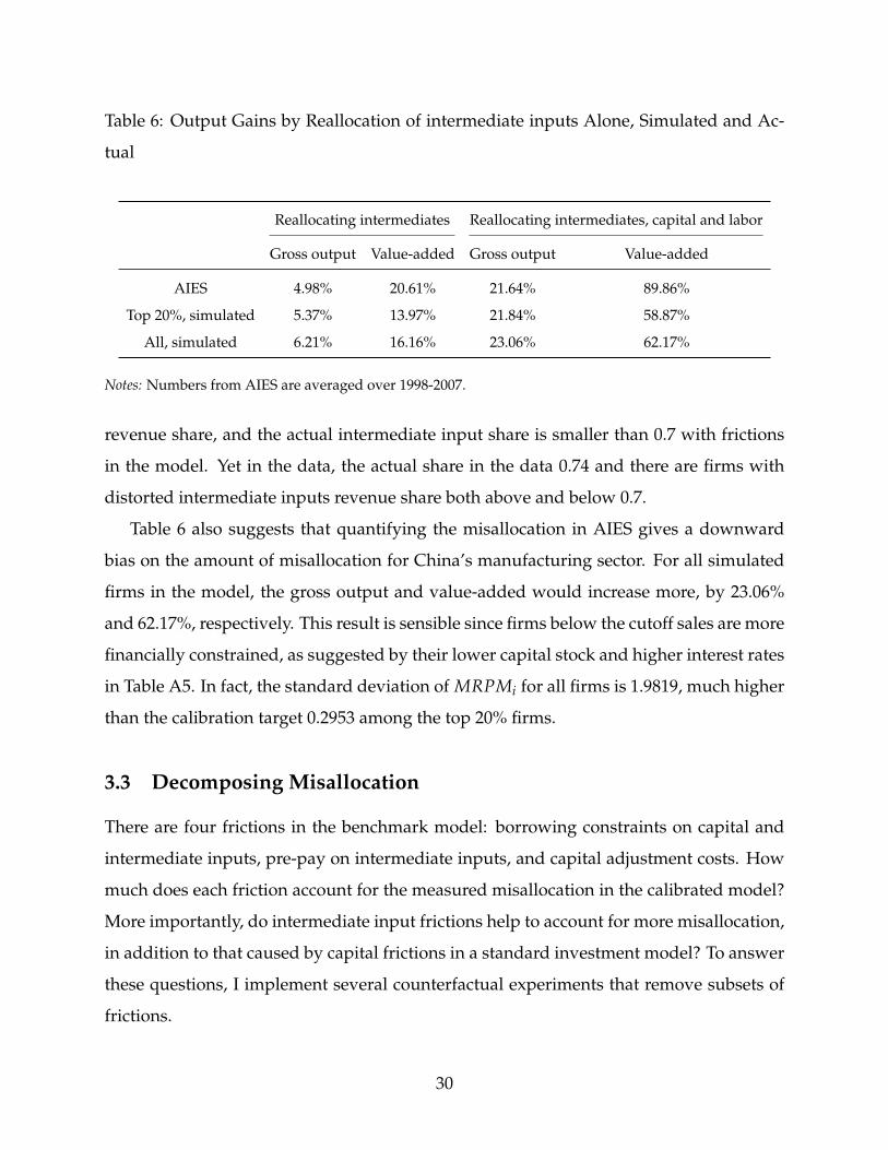
Table 6: Output Gains by Reallocation of intermediate inputs Alone, Simulated and Ac-

tual

Reallocating intermediates Reallocating intermediates, capital and labor

Gross output Value-added Gross output Value-added

AIES 4.98% 20.61% 21.64% 89.86%

Top 20%, simulated 5.37% 13.97% 21.84% 58.87%

All, simulated 6.21% 16.16% 23.06% 62.17%

Notes: Numbers from AIES are averaged over 1998-2007.

revenue share, and the actual intermediate input share is smaller than 0.7 with frictions

in the model. Yet in the data, the actual share in the data 0.74 and there are firms with

distorted intermediate inputs revenue share both above and below 0.7.

Table 6 also suggests that quantifying the misallocation in AIES gives a downward

bias on the amount of misallocation for China’s manufacturing sector. For all simulated

firms in the model, the gross output and value-added would increase more, by 23.06%

and 62.17%, respectively. This result is sensible since firms below the cutoff sales are more

financially constrained, as suggested by their lower capital stock and higher interest rates

in Table A5. In fact, the standard deviation of MRPMi for all firms is 1.9819, much higher

than the calibration target 0.2953 among the top 20% firms.

3.3 Decomposing Misallocation

There are four frictions in the benchmark model: borrowing constraints on capital and

intermediate inputs, pre-pay on intermediate inputs, and capital adjustment costs. How

much does each friction account for the measured misallocation in the calibrated model?

More importantly, do intermediate input frictions help to account for more misallocation,

in addition to that caused by capital frictions in a standard investment model? To answer

these questions, I implement several counterfactual experiments that remove subsets of

frictions.

30

The left panel of Table 7 illustrates what frictions are removed for each experiment.

Experiment 1 removes the borrowing constraints on intermediate inputs. Experiment 3

removes the borrowing constraints on capital, and Experiment 4 removes capital adjust-

ment costs. Since I embed borrowing constraints on intermediate inputs through pre-pay,

it is infeasible to remove the pre-pay friction alone. Experiment 2 then removes the bor-

rowing constraints and the pre-pay friction on intermediate inputs together. Experiment

5 removes the borrowing constraints and adjustment costs on capital. Experiment 6 re-

moves all frictions, and only retains the one-period time-to-build friction on capital. Thus,

comparing the amount of misallocation in each experiment to the benchmark model gives

the magnitude of the misallocation caused by the removed friction(s).

In this partial equilibrium framework, the levels of output, intermediate inputs, cap-

ital, and labor are not directly comparable across experiments. Thus, I quantify gross

output and value-added misallocations by computing the reallocation gains among sim-

ulated firms for each experiment, which are re-generated using calibrated parameters.

The idea is to see how much the static misallocation there would be if firms hypotheti-

cally lived in the counterfactual economy.

Table 7 presents the misallocation results on its right panel. Note that across experi-

ments, total intermediate inputs usage as a share of total gross output varies. The share

is 70% in Experiment 2 and 6 when the intermediate input frictions are absent. However,

when there are intermediate input frictions in the Benchmark model, in Experiment 3, 4,

and 5, the share drops to distorted levels smaller than 70%.28 Such a difference matters

for the value-added misallocation since it equals to gross output misallocation divided by

one net the actual intermediate input revenue share. Therefore, when I isolate misalloca-

tion caused by certain frictions, I discuss cases with the distorted αm and the undistorted

αm. The former could be viewed as purely the static misallocation, while the latter adds

28One concern is how the lower and distorted intermediate inputs share in this model reconciles with

China’s high aggregate share of intermediate inputs. Admittedly, the model is not able to generate distor-

tions τmis < 0 in Figure 1, i.e., when firms use too much intermediate inputs. The emphasis of one-sided

distortion in the model hence lowers the economy-wide revenue share. This is not contradictory to the

empirical argument that China adopts a technology that employs more intermediate inputs than other

countries.

31

extra gains by increasing total intermediate inputs to an undistorted level.

I start discussions of misallocation generated by certain friction(s) among the top 20%

firms. Comparison between Benchmark and Experiment 6 implies that one-period time-

to-build capital friction combined with stochastic productivities drives the most gross

output and value-added misallocations, about 60% and 74% in the Benchmark model,

respectively. These numbers are unexpectedly high, given the rich specification of fric-

tions in the model. However, this is generally consistent with Asker et al. (2014), which

find that the dynamic nature of capital, rather than the level of adjustment costs, accounts

most for the cross-country misallocation differences.29

If I compute the misallocation caused by each friction, Table 8 suggests that a sim-

ilar level of importance for the borrowing constraint on intermediate inputs compared

to that on capital. Differencing the Benchmark and Experiment 1 implies that an ad-

ditional 5.12% potential gross output gain when borrowing constraints on intermediate

inputs exist. The corresponding additional value-added gains with an undistorted αm

is 17.08%. These numbers are 4.89%, and 16.29% for borrowing constraints on capital.

When I use the actual distorted αm, value-added misallocation generated by the borrow-

ing constraints on intermediate inputs drops to 5.84%, because intermediate inputs rev-

enue share increases from 63% in the Benchmark model to 68% in Experiment 1. The

value-added misallocation by borrowing constraints on capital using a distorted αm does

not drop much, because intermediate inputs are also distorted in Experiment 3.

When I group frictions by the input they affect, Table 8 suggests that frictions on each

input generate about a similar magnitude of misallocation compared to borrowing con-

straints on that input. Table 8 also implies that the misallocation generated by financial

frictions could be quantitatively doubled when intermediate inputs are also affected.

If I further focus on all simulated firms instead, the magnitudes of gross output and

29In a related paper David and Venkateswaran (2019), firms receive a noisy signal of productivity shocks

for the next period, and are hence partially informed of the next period productivity in addition to the

information of current productivity zit. Firms make capital investment according to the signal. Because

of this semi-static nature of capital, their estimate of misallocation induced by pre-determined capital is

smaller than this paper.

32

value-added misallocations from four frictions are larger in row (1) of Table 8. Qualita-

tively and quantitatively, the importance of borrowing constraints on intermediate inputs

and capital in accounting for the misallocation still holds among all simulated firms.

Table 7: Simulated Gains by Equalizing Marginal Products, Benchmark and Counterfac-

tuals

B.C. Pre-pay B.C. Adj. cost Gains, top 20% Gains, all

on M on M on K on K Gross output Value-added Gross output Value-added

Data 21.64% 89.86% - -

Model

Benchmark 21.84% 58.87% 23.06% 62.17%

Exp 1 × 16.72% 53.03% 17.06% 54.15%

Exp 2 × × 16.47% 54.88% 16.47% 54.88%

Exp 3 × 16.95% 46.68% 18.45% 50.86%

Exp 4 × 20.83% 57.15% 22.73% 62.38%

Exp 5 × × 17.31% 47.48% 18.48% 50.75%

Exp 6 × × × × 13.11% 43.69% 13.25% 44.18%

Notes: B.C. on M means borrowing constraints on intermediate inputs. B.C. on K means borrowing con-

straints on capital. Pre-pay on M means pre-pay friction on intermediate inputs. Adj. costs on K means

capital adjustment costs. Cross in each cell of the left panel specifies which friction is removed from the

Benchmark model.

3.4 Discussions

This subsection discusses economic mechanisms in the benchmark model, and how I map

the current approach to the conventional value-added approach of misallocation as in

Hsieh and Klenow (2009).

Role of Intermediate Input Frictions I discuss the role of intermediate input frictions

for incumbents and entrants separately. The experiment is as follows. At t = 1, I first

sample incumbents from the stationary distribution in Experiment 2 and entrants from

the joint distribution of initial productivities and wealth.

33

Table 8: Contribution of Each Friction to Misallocation

Gains, top 20% Gains, all

Gross output Value-added Value-added Gross output Value-added Value-added

(Undistorted αm) (Distorted αm) (Undistorted αm) (Distorted αm)

All frictions (1) 8.73% 29.11% 15.18% 9.81% 32.70% 17.99%

Single friction

B.C. on M (2) 5.12% 17.08% 5.84% 6.00% 20.01% 8.02%

B.C. on K (3) 4.89% 16.29% 12.19% 4.61% 15.37% 11.31%

Adj. Cost on K (4) 1.01% 3.38% 1.72% 0.33% 1.11% -0.22%

By input

Intermediates (5) 5.38% 17.92% 3.98% 6.60% 21.99% 7.28%

Capital (6) 4.53% 15.11% 11.39% 4.58% 15.27% 11.42%

Notes: B.C. on M means borrowing constraints on intermediate inputs. B.C. on K means borrowing con-

straints on capital. Adj. costs on K means capital adjustment costs. Undistorted αm means that the aggregate

intermediate inputs as a percentage of aggregate gross output is undistorted by frictions and equals to 70%.

Distorted αm means the actual aggregate intermediate inputs revenue share in the simulated data. The en-

try of value-added misallocation in the last column of Row (4) is negative because the actual intermediate

inputs revenue share is higher in Experiment 4 than in Benchmark.

34

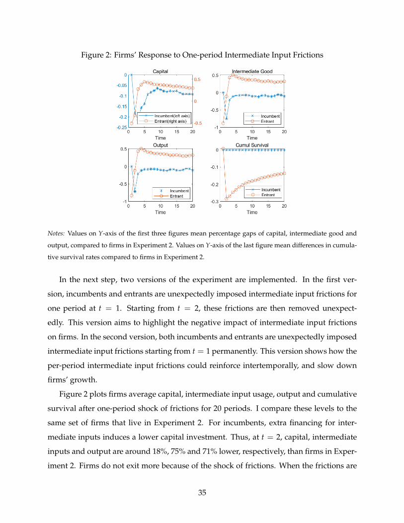
Figure 2: Firms’ Response to One-period Intermediate Input Frictions

Notes: Values on Y-axis of the first three figures mean percentage gaps of capital, intermediate good and

output, compared to firms in Experiment 2. Values on Y-axis of the last figure mean differences in cumula-

tive survival rates compared to firms in Experiment 2.

In the next step, two versions of the experiment are implemented. In the first ver-

sion, incumbents and entrants are unexpectedly imposed intermediate input frictions for

one period at t = 1. Starting from t = 2, these frictions are then removed unexpect-

edly. This version aims to highlight the negative impact of intermediate input frictions

on firms. In the second version, both incumbents and entrants are unexpectedly imposed

intermediate input frictions starting from t = 1 permanently. This version shows how the

per-period intermediate input frictions could reinforce intertemporally, and slow down

firms’ growth.

Figure 2 plots firms average capital, intermediate input usage, output and cumulative

survival after one-period shock of frictions for 20 periods. I compare these levels to the

same set of firms that live in Experiment 2. For incumbents, extra financing for inter-

mediate inputs induces a lower capital investment. Thus, at t = 2, capital, intermediate

inputs and output are around 18%, 75% and 71% lower, respectively, than firms in Exper-

iment 2. Firms do not exit more because of the shock of frictions. When the frictions are

35

Figure 3: Firms’ Response of Permanent Intermediate Input Frictions

Notes: Values on Y-axis of the first three figures mean percentage gaps of capital, intermediate good and

output, compared to firms in Experiment 2. Values on Y-axis of the last figure mean differences in cumula-

tive survival rates compared to firms in Experiment 2.

removed from t = 2, firms choose the static optimal level of intermediate inputs to max-

imize per-period profit starting from t = 3. Firms hence recover gradually in capital due

to adjustment costs and financial constraints. Starting from t = 3, capital, intermediate

inputs and output are steadily 10% lower than the levels in Experiment 2. Overall, the

negative effect of one-period intermediate good frictions is persistent.

Entrants are slightly different. Note that I impose intermediate input frictions after

they draw initial productivities and wealth when they plan for the first period production.

At t = 1 when the entrants start to produce, their capital is about 50% lower, while their

intermediate inputs and output are more than 80% lower, compared to the same set of

entrants in Experiment 2. Firms borrow more and the average borrowing increases from

128 to 376 by almost 3 times. As a result, exits increase and the cumulative survival rate

is 28% lower at t = 2, compared to Experiment 2. Such a strong cleansing effect makes

the remaining firms selectively productive. Hence, average levels of intermediate inputs

and output exceed those in Experiment 2 for the later periods.

36

In the second version of the experiment, firms are imposed intermediate input fric-

tions, starting from t = 1 permanently. Figure 3 plots average capital, intermediate input

usage, output and cumulative survival rates for 20 periods in this version. Compared to

the earlier case, incumbent firms are even smaller, and converge to an average size that

is about 60% smaller than the size of firms Experiment 2 in terms of capital, intermediate

input usage and output. The average level of capital stock for entrants grows at a much

slower rate, and converges to the level of entrants in Experiment 2 at t = 20. Because of

the intermediate input frictions, levels of intermediate inputs and output for entrants are

steadily below those in Experiment 2. Similar to Figure 2, exit rates are higher for entrants

but not for incumbents. These results suggest that the per-period intermediate input fric-

tions reinforce their negative effects intertemporally and induce a greater misallocation

in the benchmark model.

Comparison with the Value-added Approach Note that the value-added misalloca-

tion is defined as the percentage of total value-added gain when three inputs are reallo-

cated. In their seminal paper, Hsieh and Klenow (2009) use a value-added production

function, and quantify the potential value-added gain if dispersions of marginal revenue

products of capital and labor are eliminated. A natural question is that how does the

value-added misallocation under the gross output approach, compared to their numbers

given the same firm-level dataset?

To answer the question, I replicate their results using their elasticity of substitution σ =

3, cost shares of capital and labor 0.5, and the same trimming procedure. Value-added

misallocation over 1998-2007 under this approach is 93.79%, i.e., GDP would increase by

93.79% if the marginal revenue products of capital and labor were equalized. This number

is close to theirs.

Since I use σ = 6.67 in this paper, I then vary σ from 3 to 7 with the cost shares of

capital and labor unchanged. Figure 4 shows that the amount of misallocation under the

value-added approach increases quickly in the data and is very sensitive to the level of

σ. When σ = 7, value-added misallocation triples to a level of 317.71%. The monotonic

increase is due to an increasing loss caused by input misallocation when products across

37

Figure 4: value-added Misallocation by Two Approaches, Model (Benchmark) and Data

0%

50%

100%

150%

200%

250%

300%

350%

3 3.5 4 4.5 5 5.5 6 6.5 7Perentage of Value Added

 Gains from Reallocation

Elasticity of substitution σ

Value added approach (data) Gross output approach (data)

Value added approach (model) Gross output approach (model)

Notes: Log quantity and revenue productivities are trimmed by the top and bottom 1% in the data for

both approaches. In model simulated data, no trimmings are applied under the assumption that the model

should replicate variations in trimmed data. Capital and labor shares are 0.5 in the model and data. Alter-

native capital and labor shares give similar trends.

firms become more substitutable.

However, if I plot the measure of value-added misallocation under the gross output

approach, the levels decline substantially.30 Value-added misallocation is now 43% when

σ = 3 and increases to 98% when σ = 7 in the data. Figure 4 then plots the measures

of value-added misallocation in the benchmark model using the two approaches with

different σs.31 One can see that measures of value-added misallocation using the two

approaches in the model closely track those in AIES .

Why misallocation measures are substantially higher under the value-added approach?

Note that the value-added productivities TFPQvis and TFPRv

is could be written as func-

tions of the gross output productivities TFPQis, intermediate input distortion τmis , i.e.,

30A similar result is found in a recent paper by Hang et al. (2019) which put more emphasis on the input-

output linkage across sectors.31For model simulated data, I set the capital share as αk divided by one net αm and the labor share

similarly for the value-added approach. Results are similar if I set them as 0.5.

38

logMRPMis, and capital distortion τkis, i.e., logMRPKis

log(TFPQvis) = log(TFPQis)−

αsm

σ− 1τm

is +αs

kαsm

1− αsm

τkis + C1 (23)

log(TFPRvis) =

αsk

1− αsm

τkis + αs

mτmis + C2 (24)

where C1 and C2 are constants. In the appendix, I show that if logTFPQis, τkis and τm

is

follow a joint normal distribution, the measured value-added gain is

0.51− αs

m{[αs2

k (σ− 1) + αsk]VAR(τk) + [αs2

m (σ− 1) + αsm]VAR(τm) + 2αs

kαsm(σ− 1)COV(τk, τm)}

(25)

under the gross output approach, and is

0.51− αs

m{[

αs2k

1− αsm(σ− 1) + αs

k]VAR[(1− αsm + αs

mτm)τk]} (26)

under the value-added approach. In the extreme case when τmis = 0 for all firms, Equa-

tion (26) suggests that returns to capital in the value-added specification show a smaller

dispersion than VAR(τk) with the multiplier 1− αsm. Hence, the misallocation measure in

Equation (26) would be smaller, but not larger than that in Equation (25).

When intermediate input distortions exist, however, the distortion adds additional

variations to capital returns in the value-added specification. The increased VAR[(1 −

αsm + αs

mτm)τk] combined with a larger coefficient of capital αsk

(1−αsm)

in the value-added

production function pushes up the misallocation measure in (26). While intermediate in-

put distortions also increase the measure of misallocation in the second and third term

of equation (25), this effect could be smaller when VAR(τk) is sufficiently larger than

VAR(τm). In both model and data, for instance, VAR(τk) are more than 50 times as

large as VAR(τm). Because of the distortion τm, the dispersion of returns to capital in the

value-added specification, i.e., VAR[(1− αsm + αs

mτm)τk], is about the same magnitude of

VAR(τk), but not much smaller as in the case τm = 0.

The result above is not likely due to the constant supply of intermediate inputs within

each industry under the gross output approach. In the pseudo general equilibrium ex-

periment of Section 1, I show that when I increase intermediate inputs supply by λ-fold,

39

the value-added gain in fact decreases by diminishing returns. Further, it is not clear that

under the value-added approach, whether the supply of intermediate inputs increases or

decreases after reallocations because of its perfect substitutability with the value-added

bundles.

These results suggest the potential of intermediate input frictions in accounting for

the sizable misallocation found in the previous literature. Using the value-added output

measure, existing work finds dynamic models of firms hard to generate a large output

loss at a magnitude close to that in the data (e.g., Midrigan and Xu, 2014; Moll, 2014).

However, if one looks at the data through the lens of firms as gross output producers and

allows the reallocation of intermediates, the misallocation measure declines substantially

and becomes more robust to the change in elasticities of substitutions. Moreover, com-

bined with results in Section 3.3, the measured misallocation via the new lens becomes

closer to the output loss generated through dynamic models of firms with the help of ex-

plicitly modeled intermediate input frictions.

To summarize, Section 3 first calibrates the model to the AIES data, and finds that the

model well replicates measured misallocations in AIES when one reallocates intermediate

inputs alone, and along with capital and labor. Second, Section 3 finds that the misallo-

cation generated by borrowing constraints doubles when both intermediate inputs and

capital are affected. Third, Section 3 discusses how the misallocation measures using the

gross output approach compare to those using the conventional value-added approach.

4 Conclusion

Most of the existing literature on misallocation study distortions in firm-level inputs of

capital and labor. This paper introduces the intermediate input frictions and builds a

quantitative model to evaluate their relative importance in accounting for misallocation

in China’s AIES data.

This paper contributes to the literature in three folds. It first empirically quantifies

the intermediate input misallocation that are comparable to the well-understood capital

40

misallocation. Second, it shows the negative consequence of financial frictions on the

aggregate output could be doubled in a dynamic firm investment model, when finan-

cial frictions also constrain the intermediate inputs. Lastly, using the lens of firms as

gross output producers, one would obtain the potential value-added gain in a firm-level

dataset smaller than the conventional value-added approach. Combined with the second

contribution, it implies that the gap could be narrowed between the sizable misallocation

quantified in firm-level datasets and the moderate level a dynamic model generates in

the previous literature.

There are several directions for future work. First, the idea that firms may be con-

strained in intermediate inputs could be applied to other developing economies and re-

cession stages of developed economies (Kehrig, 2015). Second, this paper takes the par-

tial equilibrium framework to understand the first-order effect of intermediate input fric-

tions. One could close the economy using the input-output structure across industries.

How would this inter-sector linkage amplify output losses, following the idea of Jones

(2011)? What about the relative magnitudes of a direct output loss as in this paper, and

an indirect loss by the linkage? These questions are aligned with the research agenda in

understanding how distortions and shocks affect the GDP in an inter-connected economy

(Acemoglu, Carvalho, Ozdaglar, and Tahbaz-Salehi, 2012; Bartelme and Gorodnichenko,

2015; Osotimehin and Popov, 2020).

41

References

Acemoglu, Daron, Vasco M. Carvalho, Asuman Ozdaglar, and Alireza Tahbaz-Salehi

(2012), “The Network Origins of Aggregate Fluctuations.” Econometrica, 80, 1977–2016.

Ackerberg, Daniel A., Kevin Caves, and Garth Frazer (2015), “Identification Properties of

Recent Production Function Estimators.” Econometrica, 3, 2411–2451.

Antras, Pol, Davin Chor, Thibault Fally, and Russell Hillberry (2012), “Measuring the

upstreamness of production and trade flows.” American Economic Review, 102, 412–16.

Antras, Pol and C Fritz Foley (2015), “Poultry in motion: a study of international trade

finance practices.” Journal of Political Economy, 123, 853–901.

Asker, John, Allan Collard-Wexler, and Jan De Loecker (2014), “Dynamic Inputs and Re-

source (Mis)Allocation.” Journal of Political Economy, 122(5), 1013–1063.

Bai, Yan, Dan Lu, and Xu Tian (2018), “Do financial frictions explain chinese firms saving

and misallocation?” NBER Working Paper No. 24436.

Baqaee, David Rezza and Emmanuel Farhi (2020), “Productivity and misallocation in gen-

eral equilibrium.” The Quarterly Journal of Economics, 135, 105–163.

Bartelme, Dominick and Yuriy Gorodnichenko (2015), “Linkages and Economic Develop-

ment.” NBER Working Paper No.21251.

Bartlesman, Eric, John Haltiwanger, and Stefano Scarpetta (2013), “Cross-Country Differ-

ences in Productivity: The Role of Allocation and Selection.” American Economic Review,

103(1), 305–334.

Bento, Pedro and Diego Restuccia (2015), “Misallocation, Establishment Size, and Pro-

ductivity.” 2015 Meeting Papers. No. 1391, Society for Economic Dynamics.

Bils, Mark, Peter J. Klenow, and Cian Ruane (2017), “Misallocation or Mismeasurement?”

Working Paper.

42

Boehm, Johannes and Ezra Oberfield (2018), “Misallocation in the Market for Inputs: En-

forcement and the Organization of Production.” NBER Working Paper No. 24937.

Brandt, Loren, Gueorgui Kambourov, and Kjetil Storesletten (2018), “Barriers to Entry and

Regional Economic Growth in China.” Manuscript, University of Toronto.

Brandt, Loren, Trevor Tombe, and Xiaodong Zhu (2013), “Factor Market Distortions

across Time, Space and Sectors in China.” Review of Economic Dynamics, 16, 39 – 58.

Brandt, Loren, Johannes Van Biesebroeck, and Zhang (2014), “Challenges of Working with

the Chinese NBS Firm-level Data.” China Economic Review, 30, 339–352.

Brandt, Loren, Johannes Van Biesebroeck, and Yifan Zhang (2012), “Creative Accounting

or Creative Destruction? Firm-level Productivity Growth in Chinese Manufacturing.”

Journal of Development Economics, 97, 339–351.

Braun, Matias (2003), “Financial Contractibility and Asset Hardness.” University of

California-Los Angeles mimeo.

Broda, Christian and David E Weinstein (2010), “Product creation and destruction: Evi-

dence and price implications.” American Economic Review, 100, 691–723.

Buera, Francisco and Yongseko Shin (2013), “Financial Frictions and the Persistence of

History: A Quantitative Exploration.” Journal of Political Economy, 121(2), 221–272.

Buera, Francisco J., Joseph P. Kaboski, and Yongseok Shin (2015), “Entrepreneurship and

Financial Frictions: A Macrodevelopment Perspective.” Annual Review of Economics, 7,

409–436.

Caselli, Francesco and Nicola Gennaioli (2013), “Dynastic Management.” Economic In-

quiry, 51, 971–996.

Cooley, Thomas F. and Vincenzo Quadrini (2001), “Financial Markets and Firm Dynam-

ics.” American Economic Review, 91(5), 1286 – 1310.

Cooper, Russell W. and John C. Haltiwanger (2006), “On the Nature of Captial Adjust-

ment Costs.” Review of Economic Studies, 73, 611–633.

43

Cunat, Vicente (2007), “Trade credit: suppliers as debt collectors and insurance

providers.” The Review of Financial Studies, 20, 491–527.

David, Joel M., Hugo A. Hopenhayn, and Venky Venkateswaran (2016), “Information,

Misallocation, and Aggregate Productivity.” Quarterly Journal of Economics, 131, 943–

1005.

David, Joel M. and Venky Venkateswaran (2019), “Capital Misallocation: Frictions or Dis-

tortions?” NBER Working Paper No. 23129.

De Loecker, Jan and Frederic Warzynski (2012), “Markups and Firm-Level Export Status.”

American Economic Review, 102(6), 2437–2471.

Deloof, Marc (2003), “Does working capital management affect profitability of belgian

firms?” Journal of business finance & Accounting, 30, 573–588.

Fally, Thibault (2012), “Production staging: measurement and facts.” Boulder, Colorado,

University of Colorado Boulder, May, 155–168.

Fan, Joseph P.H. and Randall Morck (2013), Capitalising China. The University of Chicago

Press.

Fazzari, Steven M. and Bruce C. Petersen (1993), “Working Capital and Fixed Investment:

New Evidence on Financing Constraints.” The RAND Journal of Economics, 24, 328–342.

Foster, Lucia, John C. Haltiwanger, and Chad Syverson (2008), “Reallocation, Firm

Turnover, and Efficiency: Selection on Productivity or Profitability?” American Eco-

nomic Review, 98(1), 394–425.

Gandhi, Amit, Salvador Navarro, and David Rivers (2017), “How Heterogeneous is Pro-

ductivity? A Comparison of Gross Output and Value Added.” Journal of Political Econ-

omy, Forthcoming.

Gopinath, Gita, Sebnem Kalemli-Ozcan, Loukas Karabarbounis, and Carolina Villegas-

Sanchez (2017), “Capital Allocation and Productivity in South Europe.” The Quarterly

Journal of Economics, 132(4), 1915–1967.

44

Haltiwanger, John, Robert Kulick, and Chad Syverson (2018), “Misallocation Measures:

The Distortion that Ate the Residual.” NBER Working Paper No. 24199.

Hang, Jing, Pravin Krishna, and Heiwei Tang (2019), “Production Networks, Trade and

Misallocation.” Working paper.

Hopenhayn, Hugo A. (1992), “Entry, Exit, and firm Dynamics in Long Run Equilibrium.”

Econometrica, 60(5), 1127–1150.

Hopenhayn, Hugo A. (2014), “Firms, Misallocation, and Aggregate Productivity: A Re-

view.” Annual Review of Economics, 6, 735–770.

Hsieh, Chang-Tai and Peter J. Klenow (2009), “Misallocation and Manufacturing TFP in

China and India.” The Quarterly Journal of Economics, 124 (4), 1403–1448.

Jones, Charles I. (2011), “Intermediate Goods and Weak Links in the Theory of Economic

Development.” American Economic Journal: Macroeconomics, 3(2), 1–28.

Jose, Manuel L., Carol Lancaster, and Jerry L. Stevens (1996), “Corporate Returns and

Cash Conversion Cycles.” Journal of Economics and Finance, 20(1), 33–46.

Kehrig, Matthias (2015), “The Cyclical Nature of the Productivity Distribution.” Working

Paper.

Krusell, Per and Anthony A Smith (1998), “Income and wealth heterogeneity in the

macroeconomy.” Journal of Political Economy, 106, 867–896.

Manova, Kalina (2013), “Credit Constraints, Hetereogenous Firms, and International

Trade.” Review of Economic Studies, 80, 711–744.

Mendoza, Enrique G. and Vivian Z. Yue (2012), “A General Equilibrium Model of

Sovereign Default and Business Cycles.” The Quarterly Journal of Economics, 127, 889–

946.

Miao, Jianjun and Pengfei Wang (2014), “Sectoral Bubbles, Misallocation, and Endoge-

nous growth.” Journal of Mathematical Economics, 53, 153–163.

45

Midrigan, Virgiliu and Daniel Yi Xu (2014), “Finance and Misallocation: Evidence from

Plant-Level Data.” American Economic Review, 104(2), 422–458.

Moll, Benjamin (2014), “Productivity Losses from Financial Frictions: Can Self-Financing

Undo Capital Misallocation.” American Economic Review, 104(10), 3186–3221.

Oberfield, Ezra and Devesh Raval (2014), “Micro data and macro technology.” Technical

report, National Bureau of Economic Research.

Osotimehin, Sophie and Latchezar Popov (2020), “Misallocation and intersectoral link-

ages.” In Working Paper.

Peters, Michael (2013), “Heterogeneous Mark-ups, Growth and Endogenous Misalloca-

tion.” Working Paper, The London School of Economics and Political Science.

Petersen, Mitchell A. and Raghuram G. Rajan (1997), “Trade Credit: Theories and Evi-

dence.” Review of Financial Studies, 10, 661–691.

Pratap, Sangeeta and Carlos Urrutia (2012), “Financial Frictions and Total Factor Produc-

tivity: Accounting for the Real Effects of Financial Crises .” Review of Economic Dynam-

ics, 15, 336 – 358.

Raddatz, Claudio E (2003), “Liquidity needs and vulnerability to financial underdevelop-

ment.” Journal of Financial Economics, 80, 677–722.

Rajan, Raghuram and Luigi Zingales (1998), “Financial development and growth.” Amer-

ican Economic Review, 88, 559–586.

Ramey, Valerie A (1989), “Inventories as factors of production and economic fluctua-

tions.” The American Economic Review, 338–354.

Rauch, James E. (1999), “Networks versus markets in international trade.” Journal of In-

ternational Economics, 48(1), 7–35.

Restuccia, Diego and Richard Rogerson (2013), “Misallocation and Productivity.” Review

of Economic Dynamics, 16, 1–10.

46

Richards, Verlyn D and Eugene J Laughlin (1980), “A cash conversion cycle approach to

liquidity analysis.” Financial management, 32–38.

Song, Zheng, Kjetil Storesletten, and Fabrizio Zilibotti (2011), “Growing Like China.”

American Economic Review, 101, 196 – 233.

Tauchen, George (1986), “Finite State Markov-Chain Approximations to Univariate and

Vector Autoregressions.” Economics Letters, 20, 177 – 181.

Tombe, Trevor and Xiaodong Zhu (2019), “Trade, Migration, and Productivity: A Quan-

titative Analysis of China.” American Economic Review, 109, 1843 – 1872.

Tong, Hui and Shang-Jin Wei (2011), “The composition matters: capital inflows and liq-

uidity crunch during a global economic crisis.” The Review of Financial Studies, 24, 2023–

2052.

Uras, Burak R. and Ping Wang (2018), “Production Flexibility, Misallocation and Total

Factor Productivity.” NBER Working Paper No. 23970.

47

Figure A1: Entry and Exit Rates in AIES Data, Compared to Brandt et al. (2012)

(a) Entry: This Paper

0%

5%

10%

15%

20%

25%

30%

35%

40%

45%

1999 2000 2001 2002 2003 2004 2005 2006 2007

Entry Rate

(b) Entry: Brandt et al. (2012)

Appendix, as well as the construction of deflators (and the completeseries) for gross output, material inputs, and capital investment.

Employee compensation includes wages, employee supplementarybenefits, unemployment insurance, retirement benefits, health insur-ance and housing benefits. Reported compensation however appears tounderestimate total payments to labor. Labor's share of value added is

only 34.2% in our sample, compared to around 55% in the nationalincome accounts. In some of our productivity estimation, we followHsieh and Klenow (2009) and inflate wage payments by a constantfactor for all firms to work with a wage share consistent with thenational average.

Construction of a real capital stock series is difficult for two reasons:first, firms do not report fixed investment; and second, firms reportinformation on the value of their fixed capital stock at original purchaseprices. Use of nominal values runs the risk of introducing systematicbiases related to a firm's age. We develop a procedure explained in theAppendix that converts estimates at original purchase prices into realvalues that are comparable across time and firms. Our preferredbenchmark estimates imply an increase in (real) capital per worker of35.9% between 1998 and 2007, or nearly twice the growth rate impliedby official statistics. This adjustment lowers estimated productivitygrowth rates substantially, as the capital share in output in China isextremely high. Investment, which is used in the Olley–Pakes proxyestimator, is then obtained simply from theusual equation ofmotion forthe capital stock.

Finally, some firms havemissing observations for variables neededto calculate productivity. This arises either because the informationwas not originally reported, or because of negative values for variablessuch as the real capital stock or value added. We further drop all firmswith less than 8 employees as they fell under a different legal regime.As a result, 17% of the original firms are dropped from the sample in1998, but this fraction declines to 6% in each year after 2001.

4. Results

4.1. Setting the stage

There have been several growth accounting exercises carried outat themacro level that use the standard Solowmethod to estimate thecontributions of resource accumulation and productivity to growth inChina since 1978. These studies differ in terms of adjustments theymake to the official data, as well as the periods they cover. Several ofthe more widely cited studies for the entire economy includeBosworth and Collins (2008), Brandt and Zhu (2010). Chow and Li(2000), Holz (2006) and Perkins and Rawski (2008). In general theysuggest TFP growth of between 3.5 and 4.0% per annum, or more thanhalf of the growth in output per worker over the last three decades.

The role ascribed to TFP by these studies is significantly larger thanYoung (2003) finds in his widely cited article examining productivitygrowth in non-agriculture for the period between 1978 and 1998.Brandt and Zhu (2010) show how revisions by the NBS to earlier GDPfigures, and the use of a superior deflator for services raises Young'sestimate of TFP by nearly three-quarters. They also illustrate that TFPgrowth for non-agriculture was a lot higher in the 1998–2007 periodthan for the two preceding decades.

Non-agriculture includes industry, itself made up of manufactur-ing and construction, and the service sector. Estimates of servicesector productivity are limited, but the general view is that TFPgrowth has lagged that in industry as a result of less rapid marketreform and liberalization. This suggests even higher rates of TFPgrowth in industry than estimated for non-agriculture alone.

Aggregate TFP growth for the manufacturing sector can occur inthree important ways: (i) through firm-level productivity growth,(ii) exit of below-average productivity firms or entry of above-average firms, and (iii) the reallocation of production factors from lessto more productive continuing firms. Each factor will be investigatedin the following three subsections.

Chinese industry has experienced a significant amount ofrestructuring. Entry and exit is one dimension, but we might expecttransitions between ownership types or between different sub-sectors of manufacturing to be equally important. In Section 4.5, wecarry out decompositions along these lines. We also reconcile our

20%

25%

30%

35%

40%

(b) Entry

HMT &foreignprivate

0

50

100

150

200

250

300

350

0

10

20

30

40

50

60

70

80thousandsmillions

(a) Number of firms (right scale) and employment (left)

HMT &foreignprivate

collective

state

Number offirms

0%

5%

10%

15%

20%

(c) Exit

HMT &foreign

private

collective

state

0%

5%

10%

15% collective

state

1998 1999 2000 2001 2002 2003 2004 2005 2006

1999 2000 2001 2002 2003 2004 2005 2006 2007

1998 1999 2000 2001 2002 2003 2004 2005 2006 2007

Fig. 1. Employment, entry and exit by ownership type.

Table 1Summary statistics on the underlying firm-level data set.

Year Numberof firms

Valueadded

Sales Output Employment Export Net value offixed assets

1998 165,118 1.94 6.41 6.77 56.44 1.08 4.411999 162,033 2.16 6.99 7.27 58.05 1.16 4.732000 162,883 2.54 8.42 8.57 53.68 1.46 5.182001 169,030 2.79 9.24 9.41 52.97 1.61 5.452002 181,557 3.30 10.95 11.08 55.21 2.01 5.952003 196,222 4.20 14.32 14.23 57.49 2.69 6.612004 279,092 6.62 20.43 20.16 66.27 4.05 7.972005 271,835 7.22 24.69 25.16 68.96 4.77 8.952006 301,961 9.11 31.36 31.66 73.58 6.05 10.582007 336,768 11.70 39.97 40.52 78.75 7.34 12.34

Notes: all values are denoted in trillion RMB and employment in millions of workers. Allindustrial firms are included while the analysis in the paper is limited to firms in themanufacturing sector. A comparison with corresponding values in the China StatisticalYearbook, the China Statistical Abstract, and the 1995 and 2004 Census is in the onlineAppendix.

342 L. Brandt et al. / Journal of Development Economics 97 (2012) 339–351

(c) Exit: This Paper

0%

5%

10%

15%

20%

25%

1998 1999 2000 2001 2002 2003 2004 2005 2006

Exit Rate

(d) Exit: Brandt et al. (2012)

Appendix, as well as the construction of deflators (and the completeseries) for gross output, material inputs, and capital investment.

Employee compensation includes wages, employee supplementarybenefits, unemployment insurance, retirement benefits, health insur-ance and housing benefits. Reported compensation however appears tounderestimate total payments to labor. Labor's share of value added is

only 34.2% in our sample, compared to around 55% in the nationalincome accounts. In some of our productivity estimation, we followHsieh and Klenow (2009) and inflate wage payments by a constantfactor for all firms to work with a wage share consistent with thenational average.

Construction of a real capital stock series is difficult for two reasons:first, firms do not report fixed investment; and second, firms reportinformation on the value of their fixed capital stock at original purchaseprices. Use of nominal values runs the risk of introducing systematicbiases related to a firm's age. We develop a procedure explained in theAppendix that converts estimates at original purchase prices into realvalues that are comparable across time and firms. Our preferredbenchmark estimates imply an increase in (real) capital per worker of35.9% between 1998 and 2007, or nearly twice the growth rate impliedby official statistics. This adjustment lowers estimated productivitygrowth rates substantially, as the capital share in output in China isextremely high. Investment, which is used in the Olley–Pakes proxyestimator, is then obtained simply from theusual equation ofmotion forthe capital stock.

Finally, some firms havemissing observations for variables neededto calculate productivity. This arises either because the informationwas not originally reported, or because of negative values for variablessuch as the real capital stock or value added. We further drop all firmswith less than 8 employees as they fell under a different legal regime.As a result, 17% of the original firms are dropped from the sample in1998, but this fraction declines to 6% in each year after 2001.

4. Results

4.1. Setting the stage

There have been several growth accounting exercises carried outat themacro level that use the standard Solowmethod to estimate thecontributions of resource accumulation and productivity to growth inChina since 1978. These studies differ in terms of adjustments theymake to the official data, as well as the periods they cover. Several ofthe more widely cited studies for the entire economy includeBosworth and Collins (2008), Brandt and Zhu (2010). Chow and Li(2000), Holz (2006) and Perkins and Rawski (2008). In general theysuggest TFP growth of between 3.5 and 4.0% per annum, or more thanhalf of the growth in output per worker over the last three decades.

The role ascribed to TFP by these studies is significantly larger thanYoung (2003) finds in his widely cited article examining productivitygrowth in non-agriculture for the period between 1978 and 1998.Brandt and Zhu (2010) show how revisions by the NBS to earlier GDPfigures, and the use of a superior deflator for services raises Young'sestimate of TFP by nearly three-quarters. They also illustrate that TFPgrowth for non-agriculture was a lot higher in the 1998–2007 periodthan for the two preceding decades.

Non-agriculture includes industry, itself made up of manufactur-ing and construction, and the service sector. Estimates of servicesector productivity are limited, but the general view is that TFPgrowth has lagged that in industry as a result of less rapid marketreform and liberalization. This suggests even higher rates of TFPgrowth in industry than estimated for non-agriculture alone.

Aggregate TFP growth for the manufacturing sector can occur inthree important ways: (i) through firm-level productivity growth,(ii) exit of below-average productivity firms or entry of above-average firms, and (iii) the reallocation of production factors from lessto more productive continuing firms. Each factor will be investigatedin the following three subsections.

Chinese industry has experienced a significant amount ofrestructuring. Entry and exit is one dimension, but we might expecttransitions between ownership types or between different sub-sectors of manufacturing to be equally important. In Section 4.5, wecarry out decompositions along these lines. We also reconcile our

20%

25%

30%

35%

40%

(b) Entry

HMT &foreignprivate

0

50

100

150

200

250

300

350

0

10

20

30

40

50

60

70

80thousandsmillions

(a) Number of firms (right scale) and employment (left)

HMT &foreignprivate

collective

state

Number offirms

0%

5%

10%

15%

20%

(c) Exit

HMT &foreign

private

collective

state

0%

5%

10%

15% collective

state

1998 1999 2000 2001 2002 2003 2004 2005 2006

1999 2000 2001 2002 2003 2004 2005 2006 2007

1998 1999 2000 2001 2002 2003 2004 2005 2006 2007

Fig. 1. Employment, entry and exit by ownership type.

Table 1Summary statistics on the underlying firm-level data set.

Year Numberof firms

Valueadded

Sales Output Employment Export Net value offixed assets

1998 165,118 1.94 6.41 6.77 56.44 1.08 4.411999 162,033 2.16 6.99 7.27 58.05 1.16 4.732000 162,883 2.54 8.42 8.57 53.68 1.46 5.182001 169,030 2.79 9.24 9.41 52.97 1.61 5.452002 181,557 3.30 10.95 11.08 55.21 2.01 5.952003 196,222 4.20 14.32 14.23 57.49 2.69 6.612004 279,092 6.62 20.43 20.16 66.27 4.05 7.972005 271,835 7.22 24.69 25.16 68.96 4.77 8.952006 301,961 9.11 31.36 31.66 73.58 6.05 10.582007 336,768 11.70 39.97 40.52 78.75 7.34 12.34

Notes: all values are denoted in trillion RMB and employment in millions of workers. Allindustrial firms are included while the analysis in the paper is limited to firms in themanufacturing sector. A comparison with corresponding values in the China StatisticalYearbook, the China Statistical Abstract, and the 1995 and 2004 Census is in the onlineAppendix.

342 L. Brandt et al. / Journal of Development Economics 97 (2012) 339–351

Notes: Entrants (exits) include (1) firms enter into (exit from) production as in the model; (2) firms grow

above (decline below) 5 million threshold sales.

Appendix

Matching Firms across Years AIES is cross-sectional and requires matching of firms

over time to understand the dynamics. I match firms across years based on codes in

Brandt et al. (2012) with some modifications. Firms are matched sequentially accord-

ing to their registration IDs, names, a string that combines names of legal representa-

tives, industry and area codes, a string that combines phone numbers, industry and area

codes, and lastly a string that combines opening year, geographic code, industry, town-

ship/streets/villages and product names. Entry and exit rates in the merged data are

plotted in Figure A1 in comparison to Brandt et al. (2012). One can see that matching re-

sults are close. Note that entries and exits in the AIES data are not equivalent to those in

48

the model. I also use the same perpetual inventory method from their paper to construct

the firm-level real capital stock over time.

One-Input Reallocation This appendix introduces how Section 1.2 calculates gross

output and value-added gains by reallocating one input at a time. To simplify the nota-

tion, I use Ais to represent exp(zis) in the paper. Note the industry-level ¯TFPRs

¯TFPRs =PsYs

Kαs

ks L

αsl

s Mαsm

s

=∑Ns

i=1 PisYis

Kαs

ks L

αsl

s Mαsm

s

(27)

and hence the industry-level productivity

TFPs =Ys

Kαs

ks L

αsl

s Mαsm

s

= ¯TFPRs/Ps

= ¯TFPRs(Ns

∑i=1

(Ais

TFPRis)σ−1)

1σ−1

=(Ns

∑i=1

(Ais¯TFPRs

TFPRis)σ−1)

1σ−1

=(Ns

∑i=1

(Ais¯MRPK

αsk

s ¯MRPMαsm

s¯MRPL

αsl

s

MRPKαs

kis MRPMαs

mis MRPL

αsl

is

)σ−1)1

σ−1 (28)

Note that Ais =R

σσ−1is

Kαs

kis L

αsl

is Mαsm

is

(Pσs Ys)

− 1σ−1 , where Ris is firm-level gross output revenue in the

data. According to Equation (28), industry TFPs in the data could be computed with a

multiplier (Pσs Ys)

− 1σ−1 .

If only intermediate inputs are reallocated to equalize its marginal revenue products

within industries, ¯MRPMs = MRPMis holds after the reallocation. The reallocation,

however, changes the firm-level gross output revenue

R′is = (PisYis)′ = AisK

αsk

is Lαs

lis M

′αsm

is (Y′s P′σs )

1σ (29)

where R′is or (PisYis)′, M′is, Y′s , and P′s denote revenue, intermediate inputs, industry-level

output quantity, industry-level price after the reallocation. Firm-level and industry-level

marginal revenue products of capital and labor also change accordingly. The co-movement

of industry- and firm-level marginal products helps to cancel out (Y′s P′σs )

1σ in equation (28)

49

after reallocation. The new industry TFPs is

TFP′s = (Ns

∑i=1

(Ais¯MRPK

′αsk

s ¯MRPL′αs

ls

MRPK′αs

kis MRPL

′αsl

is

)σ−1)1

σ−1 (30)

where MRPX′ is the new marginal product, x = K, L. Thus, gross output gain for indus-

try s is

TFP′s/TFPs − 1 (31)

which cancels out (Pσs Ys)

− 1σ−1 in both Aiss in the numerator and in the denominator. The

economy-wide gross output gain is an industry gross output weighted gains

S

∑s=1

θsTFP′s/TFPs − 1 (32)

Gross output gains from reallocating capital or labor are computed similarly.

To compute the value-added gain, note that the industry-level value-added VAs

VAs = Ys −Ms (33)

The economy-wide value-added gain after reallocating intermediate inputs is

∏Ss=1(Y

′s)

θs −∏Ss=1(Ys)θs

∏Ss=1(Ys)θs −∑S

s=1 Ms(34)

The numerator is the gross output gain, and the denominator is the value-added before

the reallocation. Note

∏Ss=1 Yθs

s

∑Ss=1 Ms

=P ∏S

s=1 Yθss

P ∑Ss=1 Ms

=∑S

s=1 PsYs

P ∑Ss=1 Ms

=1

αm(35)

The second equation holds because of the zero-profit condition for the Cobb-Douglas

aggregator, and αm is the economy-wide intermediate inputs revenue share. Therefore,

the value-added gain is

S

∑i=1

θs

1− αm(TFP′s/TFPs − 1) (36)

50

Misallocation in FHS(2008) Industries This appendix quantifies the input misallo-

cation in industries that feature a homogeneous output studied in Foster et al. (2008). I

exclude white pan bread, roasted coffee beans, and oak flooring since these products are

not consumed much by Chinese households over 1998-2007. Since the finest 4-digit CIC

industries are still coarser than these products, I keep firms that report the product as

what they produce and what they only produce using the information from three vari-

ables, Main Product 1, Main Product 2 and Main Product 3 in AIES. For example, I keep

firms that report their Main Product 1 variable as the Chinese translation of Corrugated

& Solid Fiber Boxes, i.e., Zhi Xiang, and their Main Product 2 and 3 missing. The product

of gasoline is dropped since numbers of firms that uniquely produce gasoline are fewer

than 10 for most years.

Financially Vulnerable Measures Table A2 lists asset tangibility and external finance de-

pendence measures for 28 2-digit industries. Figure A2 plots coefficients of variations in

MRPMist against these financially vulnerable measures in the year of 2004.

Table A1: Input Misallocation in Foster et al. (2008) Industries

Gross output gains Value-added gains

Intermediates Capital Labor Intermediates Capital Labor

Corrugated & Solid fiber Boxes 4.51% 4.57% 1.89% 17.81% 16.78% 6.81%

Carbon Black 3.13% 3.15% 1.08% 11.77% 11.63% 3.89%

Ready Mixed Concrete 4.31% 3.77% 2.20% 15.83% 14.03% 8.35%

Plywood 1.21% 21.67% 2.19% 3.35% 55.05% 6.21%

Sugar 6.23% 1.77% 0.47% 33.99% 9.66% 2.83%

Note: Misallocation measures are gains obtained when reallocating one input at a time, using the same

method as in Table 1. Numbers are averaged from 1998 to 2007. The year of 2002 for carbon black and

sugar is dropped for intermediate inputs, since gains are much higher than the rest of years. For the same

reason, the year of 1998 for ready mixed concrete is dropped.

51

Table A2: Asset Tangibility and External Finance Dependence Measures in 2-digit CIC

Industries

2-digit Industry Name Asset External

CIC Code Tangiblities Finance Dependence

13 Primary Food Processing 0.3777 0.1368

14 Manufacture of food 0.3777 0.1368

15 Manufacture of beverage 0.2794 0.0772

16 Manufacture of tobacco 0.2208 -0.4512

17 Manufacture of textile 0.3730 0.4005

18 Garments and products 0.1317 0.0286

19 Leather, furs and down products 0.0906 -0.1400

20 Timber processing 0.3796 0.2840

21 Manufacture of furniture 0.2630 0.2357

22 Paper making and products 0.5579 0.1756

23 Printing and publishing 0.3007 0.2038

25 Petroleum refineries 0.6708 0.0420

26 Raw chemical materials 0.4116 0.2050

27 Medical and pharmaceutical products 0.1973 0.2187

28 Chemical fiber 0.1973 0.2187

29 Rubber products 0.3790 0.2265

30 Plastic products 0.3448 1.1401

31 Nonmetal mineral products 0.4200 0.0620

32 Ferrous metals 0.4581 0.0871

33 Nonferrous metals 0.3832 0.0055

34 Metal products 0.2812 0.2371

35 Ordinary machinery 0.1825 0.4453

37 Transport equipment 0.2548 0.3069

39 Electric equipment and machinery 0.2133 0.7675

40 Electronic and telecom equipment 0.2133 0.7675

41 Professional and scientific equipment 0.1511 0.9610

42 Other manufacturing 0.1882 0.4702

Notes: Numbers are from Table I in Braun (2003).

52

Figure A2: Industry-level Dispersion of Marginal Revenue Products of Intermediates,

Financial Vulnerabilities and Operating Cycles, Year 2004

131415

16

17

1819

2021

22

23

242526

27

2829

3031 323334

35

36 3739

40

41

42

0.2

.4.6

.8d

isp

_m

rpm

0 .2 .4 .6 .8Asset Tangibility

131415

16

17

1819

2021

22

23

2425 26

27

2829

3031323334

35

3637 39

40

41

42

0.2

.4.6

.8d

isp

_m

rpm

0 .5 1 1.5External Finance Dependence

1314

15

16

17

18

1920

212223 24

25

2627

28

2930

31

32

33

34 35

36

37 39

40

41

42

23

45

67

dis

p_

mrp

m

0 .5 1 1.5 2Cash Coversion Cycle

131415

16

17

1819

2021 22

23

242526

27

2829

3031 3233

3435

363739

40

41

42

0.2

.4.6

.8d

isp

_m

rpm

1 1.5 2 2.5Dispersion of Capital Returns

Note: disp mrpms for industry s is the standard deviation of MRPMis standardized by its

industry-level mean, after trimming the top and bottom 1%. Measures of asset tangibility

and external finance dependence are from Braun (2003) and Rajan and Zingales (1998)

that use the Compustat data. Year 2004 is an example but results are similar for other

years.

Table A3: Output, Capital, Employment and Firm Age in AIES and Census, 2004

AIES Census

Mean S.D. Mean S.D.

Sales 39,626.59 74,143.66 6,643.77 17,272.79

Capital 16,465.49 37666.58 2,847.01 8,108.27

Employment 223 740 64 343

Age 8.22 10.14 6.48 8.11

Number 252,095 1,255,707Notes: Sales and capital are in 1000 yuan, current price.

53

Table A4: Entry in AIES Dataset over 5 Years

China

1998-2003 2002-2007

Number of Firms, End Year

AIES Incumbents 39.90% 30.27%

AIES Entrants (Age > 5) 23.32% 24.67%

AIES Entrants (Age ≤5) 36.77% 45.06%

Market Share, End Year

AIES Incumbents 60.45% 57.34%

AIES Entrants (Age > 5) 14.66% 14.07%

AIES Entrants (Age ≤5) 24.89% 28.59%

AIES and Census 2004 The AIES data 1998-2007 has a threshold sales of 5 million

yuan. Table A3 describes the differences between AIES and the Economic Census 2004.

One can see that AIES firms are the largest 20% of all manufacturing firms in the Census.

Average sales, capital, and employment in AIES are almost six times as large as those in

the Census data. Firms in the Census are also younger on average. Nevertheless, AIES

produces about 90% of manufacturing output and employs 70% of workers.

Inventory Model This appendix presents an alternative framework that models the

inventory stock of intermediate inputs, and hence the purchases and consumptions of

intermediates as positive and negative changes of this inventory.

Let the state variable m now be the intermediate input inventory. Suppose that in the

current period, the firm makes ∆m′ intermediates investment and uses m for productions.

The intermediate inventory for the next period is hence m′ = m− m + ∆m′ when there is

no inventory holding cost or no wearing out.

Because the firm still needs to pay (1−ω)∆m in this period, purchase of intermediate

inputs in the previous period ∆m becomes the additional state variable. Given the whole

54

state vector (z, b, k, m, ∆m), value of continuation is

Vc(z, b,k, m, ∆m) = maxb′,k′,∆m′maxm≤m{py(m)− (1−ω)∆m + m− m}+ (1− δ)k−ω∆m′ − k′ − C(k, k′)− b+

q′b′ − co + βEz′|zV(z′, b′, k′, m′, ∆m′)

s.t. maxm≤m{py(m)− (1−ω)∆m + m− m}+ (1− δ)k−ω∆m′ − k′ − C(k, k′)− b + q′b′ − co ≥ 0

m′ = m− m + ∆m′

q′b′ ≤ Ez′|zV0(z′, k′) (No Ponzi-Game) (37)

Although the original model is not differentiable near the hyperplane where Vx =

Vc, I add a stochastic shock Θ ∈ [Θ, Θ] to the value of exit, Vx, to make the problem

differentiable here for an ease of exposition, i.e.,

Vx(z, b, k, m, ∆m) = max{γ2maxm≤m{py(m)− (1−ω)∆m + m− m} − b[1(b ≤ 0)γ2 + 1(b > 0)]

+ γ1(1− δ)k, Θ} (38)

One can show that first-order conditions for the choice of ∆m′ in this problem are

the same as those for the next period intermediate inputs m′ in the original model. Fur-

thermore, the value of exit also keeps unchanged when m = ∆m, and increases when

m > ∆m compared to the original model. For the value of continuation, again dividend

in this period keeps unchanged when m = ∆m, and increases when m > ∆m that would

alleviate borrowing constraints and the pre-pay friction. This channel increases the value

of continuation because of the additional inventory dimension firms could choose. Since

m > ∆m happens more often when productivity z−1 in the previous period is low, the ex-

tent on how much the inventory channel would alleviate borrowing constraints is likely

to be small, especially if I further add an inventory holding cost. Hence, I use the original

model for keeping the number of state variables small to avoid the curse of dimensional-

ity in computation.

Computations The model is a partial equilibrium one since (i) there are no market

clearings for final output and intermediate inputs, neither for capital and labor; (ii) the

prime interest rate is exogenously given as in a small open economy. The partial equi-

librium framework makes the computation relatively inexpensive, compared to a general

equilibrium models a la Krusell and Smith (1998).

55

The computation has three parts: (i) value function iterations; (ii) finding a stationary

firm size distribution (FSD); (iii) simulation based on FSD.

Value function iterations are computed in the following step:

1. Compute the value of continuation Vc as the maximum value when there are no

financial frictions;

2. Let the initial guess Vc0 = Vc. Note that one needs to guess from a value function

higher than the true one everywhere because of the endogenous borrowing con-

straint and the existence of debt upper limit when the break-even interest rate might

approach infinite;

3. Given Vc0 and Vx as in the paper, compute optimal b′, k′, m′ and ensure that con-

straints of non-negative dividends and no Ponzi-Game are satisfied;

4. Update the value function and repeat 3 until the convergence criterion ||Vcn+1 −

Vcn || < ε is satisfied.

I then iterate to obtain a stationary firm size distribution on grids of debt, capital, inter-

mediate inputs, and productivities. This distribution is then used to sample incumbent

firms. Combined with a mass of µent entrants sampled from initial debt and productivity

distributions, one could obtain an AIES-alike unbalanced panel of firms that the realloca-

tion exercises are based on.

I use gfortran 7.5 and OpenMPI 4.0.1 for parallel computations that employ 80 work-

ers at a time. The number of grids is 5 for permanent productivities, 15 for transitory

productivities, 16 for debt/saving, 16 for capital, 40 for intermediate inputs. The whole

running time is 10 hours for each parameterization.

Constrained Firms in the Model and in the Data Firms with an MRPMi greater than

1 in the model either have unexpected high productivities because of the pre-pay, or are

financially constrained and under-invest in intermediate inputs. In the latter case, if the

model well captures the data, one would expect that firms with MRPMi > 1 in the model

and their counterparts in the data are similar. Table A5 thus compares the levels of capital

56

Table A5: Average Productivity, Capital and Interest Rates, Constrained and Uncon-

strained

AIES Top 20%, Simulated All, Simulated

Constrained Unconstrained Constrained Unconstrained Constrained Unconstrained

Log TFPQ 2.14 1.89 1.89 1.58 1.15 1.21

Capital Stock 23,153.83 24,373.31 1720.03 2715.37 308.05 1187.64

Interest Rate 6.43% 4.02% 6.20% 6.19% 267.66% 8.94%

Notes: Constrained firms have MRPMi > 1, and unconstrained ones have MRPMi ≤ 1. Statistics in AIES

are calculated first for each year, and are then averaged over 1998-2007. In AIES, capital stock are in constant

1998 thousand yuan, and interest rates are calculated by interest expenses divided by total liabilities.

stock, productivity and interest rates between firms with MPRMit > 1 (constrained) and

those with MRPMit ≤ 1 (unconstrained), both in the model and in the data. To remove

the impact of state-owned firms, I restrict to the non-state-owned sector in AIES. And

to meaningfully discuss financial constraints, I restrict my model-simulated data to the

subsample of firms with debt, excluding firms that save.

The model resembles AIES in several aspects. Constrained firms, on average, have

higher productivities, lower capital stocks, and pay higher interest rates both in the data

and in the simulated top 20% subsample. For TFPQ, constrained firms are 25% and 31%

more productive than unconstrained one in the data and in the model, respectively. The

model delivers this phenomenon of size-dependent distortions because of a higher de-

mand in intermediate inputs for more productive yet financially constrained firms. Firms

whose sales are below the cutoff are less productive, and might be constrained for a dif-

ferent reason: their inability to generate cash flows from productions. Hence, for the

entire simulated sample, constrained firms are actually 6% less productive than uncon-

strained ones. But this does not eliminate the size-dependent distortions. Correlation

between marginal revenue products of intermediate inputs and productivity in the entire

sample is still positive and equals to 0.02, although much smaller than 0.58 in the top 20%

subsample.

For capital stock, constrained firms are 5% and 36% smaller than unconstrained firms

57

in the data and in the top 20% subsample, respectively.32 Accordingly, constrained firms

pay interests rates that are 2.41% and 0.01% higher in the data and in the model. The phe-

nomenon of a lower capital stock and higher interest rates for constrained firms is more

pronounced in the entire simulated sample.

Value-added Misallocation: Two Approaches This appendix shows that misalloca-

tion measures, i.e., value-added gains through reallocations, differ under value-added

and gross output approaches when the elasticity of substitution σ is finite.

Let me denote Avis and TFPRv

is as firm-level TFPQ and TFPR under the value-added

approach. The corresponding industry-level TFPQ and TFPR are Avs and ¯TFPRv

s . Note

log(Avis) = log(

PisYis − PMis

Pis)−

αsk

1− αsm

log(Kis)−αs

l1− αs

mlog(Lis) (39)

log(TFPRvis) = log(PisYis − PMis)−

αsk

1− αsm

log(Kis)−αs

l1− αs

mlog(Lis) (40)

and αsk + αs

l + αsm = 1− 1

σ , αsk + αs

l + αsm = 1.

Using the property of Cobb-Douglas functions

log(PisYis − PMis) = log(PisYis − (1− τis)PM∗is)

= log(PisYis − (1− τis)αsmPisYis)

≈ log(PisYis)− (1− τis)αsm (41)

where M∗is is the static optimal level of intermediate inputs, of which the revenue share

shall equal to αsm in a Cobb-Douglas production function. τm

is , or logMRPMis equivalently,

measures the idiosyncratic distance of actual intermediate inputs usage from the optimal

level. Plugging this equation back to (39) and (40), the followings hold

log(Avis) =

11− αs

mlog(Ais)−

αsm

(1− αsm)(σ− 1)

logMis + {αsm −

αsm

1− αsm

σ

σ− 1}τm

is + C′1

(42)

32In AIES, there is a time trend that constrained firms become increasingly smaller relative to the uncon-

strained ones in terms of capital stock. For instance, constrained firms are 9% larger in 1998. But in 2007,

constrained firms are 23% smaller compared to the unconstrained ones, presumably because more smaller

firms enter as economic reforms deepen.

58

log(TFPRvis) =

11− αs

mlog(TFPRis) + {αs

m −αs

m1− αs

m}τm

is + C′2 (43)

where C′1 and C′2 are constants in terms of αsm, σ, aggregate price P and aggregate output Y.

The economic intuition of the second term in Equation (42) is that the monopolistic firms

charge markups over the marginal cost of intermediate inputs when they produce gross

output, which is absent when firms are modeled as value-added producers that charge

markups only over the marginal costs of capital and labor. Analogously, the industry-

level ¯TFPRvs is

log( ¯TFPRvs ) =

11− αs

mlog( ¯TFPRs) + {αs

m −αs

m1− αs

m}τm

s + C′2 (44)

where τms is the industry average distortion on intermediate inputs.

Note that misallocation, i.e., the potential value-added gain through reallocations, is

quantified by

log(TFPvs,e f f )− log(TFPv

s ) = log{Ns

∑i=1

(Avis)

σ−1}1

σ−1 − log{(Ns

∑i=1

(Avis

¯TFPRvs

TFPRvis)σ−1)

1σ−1} (45)

under the value-added approach, and by

11− αs

m{log(TFPs)− log(TFPs,e f f )} =

11− αs

m{log{

Ns

∑i=1

Aσ−1is }

1σ−1 − log{(

Ns

∑i=1

(Ais¯TFPRs

TFPRis)σ−1)

1σ−1}}

(46)

under the gross output approach. Hence, equations (45) and (46) are equal when σ = ∞,

and both measures of misallocations approach infinity since only the most productive

firms shall produce all goods at a constant return to scale after reallocations.

In a more realistic case when σ < ∞, one can show that the value-added TFPQ and

TFPR can be expressed by the model primitives

log(Avis) = log(Ais)−

αsm

σ− 1τm

is +αs

kαsm

1− αsm

τkis + C1 (47)

log(TFPRvis) =

αsk

1− αsm

τkis + αs

mτmis + C2 (48)

59

when C1 and C2 are constants, and τkis is the capital wedge logMRPKis. Note how distor-

tions enter into the value-added quantity productivity. The following results are useful

in deriving these equations

(1− τkis)

1−αl−αm(1− τmis )

αmσ− 1

σA

σ−1σ

is K−1σ

is ∝ r

⇒ Kis ∝ (1− τmis )

αmσ(1− τkis)

(1−αl−αm)σ Aσ−1is

⇒ Mis ∝ Kis1− τm

is

1− τkis

∝ (1− τmis )

αmσ+1(1− τkis)

(1−αl−αm)σ−1Aσ−1is (49)

Now I use the model primitives to derive the analytical expressions of misallocation

measures under both approaches. Note the industry TFPR

¯TFPRs = ( ¯MRPKs)αs

k( ¯MRPMs)αs

m

= [Ns

∑i=1

PisYis

PsYs(1− τk

is)]−αs

k [Ns

∑i=1

PisYis

PsYs(1− τm

is )]−αs

m (50)

where ¯MRPKs is defined as αskPsYs/Ks, and ¯MRPMs as αs

mPsYs/Ms. Given Kis, Mis and

the monopolistic competition market structure, one can show that

PisYis

PsYs∝

Aσ−1is (1− τk

is)αs

k(σ−1)(1− τmis )

αsm(σ−1)

∑Nsi=1 Aσ−1

is (1− τkis)

αsk(σ−1)(1− τm

is )αs

m(σ−1)(51)

Assume that ais = log(Ais), τmis and τk

is follow a multivariate normal distribution with a

variance-covariance matrix ∑. I allow covariances between ais and τs, and the covariance

between τs be nonzero. The industry average TFPR can be expressed by

¯TFPRs = exp{σ− 1}exp{(αskµτk + αs

mµτm)− (αs2k (σ− 1) + 0.5αs

k)VAR(τk)− (αs2m (σ− 1) + 0.5αs

m)VAR(τm)

− (σ− 1)αskCOV(a, τk)− (σ− 1)αs

mCOV(a, τm)− 2αskαs

m(σ− 1)COV(τk, τm)}

(52)

by applying moment generating functions for multivariate normal distributions. Hence,

the potential value-added gain under the gross output approach is

11− αs

m{0.5(αs2

k (σ− 1) + αsk)VAR(τk) + 0.5(αs2

m (σ− 1) + αsm)VAR(τm) + αs

kαsm(σ− 1)COV(τk, τm)}

(53)

60

and the covariance terms between a and τs are canceled out. Similarly, the potential

value-added gain under the value-added approach is

0.5{[αs2

k(1− αs

m)2 (σ− 1) +

αsk

(1− αsm)

]VAR[(1− αsm + αs

mτm)τk]} (54)

where αsk

(1−αsm)

is the cost share of capital in a value-added production function, and (1−

αsm + αs

mτm)τk is the firm-level value-added marginal revenue product logMRPKv. It can

be seen that intermediate inputs distortion adds another dimension of variation to returns

to capital in a value-added specification. When the dispersion of τm increases, it is likely

that equation (54) is going to increase faster with the first coefficient αs2k

(1−αsm)2 . However, it

is hard to tell the relative magnitude in algebra and hence this paper turns to the data for

the answer.

61