Intermediate Inputs and the Export Gravity Equation Antonio Navas Francesco Serti Chiara Tomasi ISSN 1749-8368 SERPS no. 2013014 Originally Published: October 2013 Updated: March 2015

Intermediate inputs and the export gravity equation ∗†

Antonio Navasa, Francesco Sertib, and Chiara Tomasic

aDepartment of Economics, University of SheffieldbDepartamento de Fundamentos del Analisis Economico, Universidad de Alicante.

cUniversity of Trento, Italy, and LEM, Scuola Superiore Sant’Anna, Italy

March 24, 2015

Abstract

This paper proposes a theoretical micro-foundation for the export gravity equation at thefirm-level in the presence of imports in intermediates. By increasing a firm’s productivity,importing intermediate inputs influences export decisions, both at the extensive and the intensivemargins. In the model, market size and distance shape the effects that imports have on a firm’sproductivity. It follows that an increase in foreign market size or a decline in transportationcosts exert, besides the standard direct impact, an indirect positive effect on export profitabilitythrough a firm’s efficiency increase induced by the imports of intermediate inputs. Exploitingdata on product-destination level transactions of a large panel of Italian firms, the paper providesempirical evidence in support of the predictions of the model.

JEL codes: F12, F14

Keywords: Imports, Exports, Firm heterogeneity, Gravity equation.

∗Corresponding author : Francesco Serti, Department of Economics (FAE) University of Alicante Campus de SanVicente, 03690 Alicante, Spain E-mail francesco.serti@gmail.com, Tel +34 965 903614.†The present work has been possible thanks to a research agreement between the Italian Statistical Office (ISTAT)

and the Scuola Superiore Sant’Anna. We thank the participants of the ISGEP 2012, the European Trade Study Group(ETSG 2013), the European Economic Association Meeting (EEA) (2014) and the seminars of the University ofGottingen, Siena and Barcelona for their numerous comments and stimulating suggestions. Francesco Serti gratefullyacknowledges financial support from from the Spanish Ministries of Education and Science and Economics andCompetitiveness (ECO2012-34928).

1

1 Introduction

A growing empirical and theoretical literature has emphasised the importance of firm heterogeneityin trade. The burgeoning studies on international trade have mostly focused on exports, whileimports have been relatively neglected. Even less attention has been given to firms engaged in acombination of both imports and exports. This is quite surprising given the increasing internationalfragmentation of production, implying that more and more firms are active in both imports andexports of intermediates and final goods (Hummels et al.; 2001). Only very recently new researchhas started combining information on both the import and export sides. The available studies showthat the majority of exporters are also importers and vice versa. These firms, which have beenlabeled as two-way traders, account for the bulk of a country’s total trade (Bernard et al.; 2007;Mayer and Ottaviano; 2008; Muuls and Pisu; 2009; Castellani et al.; 2010).

We contribute to this new strand of literature by investigating previously unexplored effectsof the connection between an individual firm’s import and export outcomes. The paper studiesthe influence that the complementarity between the two trade activities has on the export gravityequation, at the firm level. The basic form of the gravity equation relates exports to the economicsize and the geographical distance of the destination market, with the latter used as a proxy fortransportation costs. The recent trade models with heterogeneous firms show that the gravity forcesaffect exports via both the extensive and intensive margins of trade (Melitz; 2003; Chaney; 2008;Helpman et al.; 2008). Accordingly, higher market size or lower distance increase the probabilitythat a firm exports to a particular destination as well as its export value to that market.1 However,whether a firm is importing or not may be relevant to evaluate the overall impact that market sizeand distance have on its export patterns.

This paper derives and estimates the export gravity equation for both the extensive and intensivemargins of trade among asymmetric countries in the presence of imports in intermediate inputs.Our theoretical framework follows Chaney (2008) which derives the export gravity equation for finalgoods in a model of trade with firm heterogeneity. As in Chaney (2008) countries are asymmetricand differ in terms of size, labour costs, trade and institutional barriers. In addition, our modelintroduces an intermediate input sector. To produce, firms in the final good sectors use laborand a continuum of intermediate inputs from different locations. The technology is similar toearly endogenous growth models (Romer; 1990; Rivera-Batiz and Romer; 1991), which use a CobbDouglas specification in which there is love of variety in intermediate inputs.

Relevant implications emerge from our setting. In line with previous theoretical frameworksand empirical analyses, the model predicts that importing increases a firm’s productivity, througha better reallocation of resources across new intermediate inputs.2 The model shows that therelatively more productive firms self select into importing and that only a subset of the mostproductive firms undertake both trade activities.3

More importantly, our theoretical framework emphasizes that the positive effect of importing on

1As suggested in Crozet and Koenig (2010), the definition employed in this paper for the intensive margin ofexport reflects that used in Chaney (2008), that is the value shipped by the marginal exporter, which differs fromthe average shipment per exporter, used in most empirical analyses (Eaton et al.; 2004; Bernard et al.; 2007; Mayerand Ottaviano; 2008).

2For a theoretical background of the productivity gains induced by intermediate inputs see Markusen (1989);Grossman and Helpman (1991); Acharya and Keller (2009) among others. Micro-level empirical studies providingevidence on the positive relationship between import and a firm’s productivity include Kasahara and Rodrigue (2008)for Chile, Halpern et al. (2011) for Hungary, Amiti and Konings (2007) for Indonesia. Similarly, Goldberg et al. (2010)find that an increase in imported input varieties contribute to the expansion in domestic firms’ product scope.

3As stressed by Kasahara and Lapham (2013) the evidence points as the presence of fixed costs not only ofexporting but also of importing, and to a process of self-selection in both export and import markets.

2

a firm’s productivity depends on both the mass of imported intermediate inputs available, as wellas the price of each intermediate. Bigger markets provide a larger variety of inputs, while closercountries charge lower prices because of lower transportation costs. This implies that importingfrom closer and larger markets has a stronger effect on a firm’s productivity and thereby it rises afirm’s probability of exporting, as well as its export value. Therefore, the standard gravity forcesgoverning a firm’s decision to export also determine the heterogeneous productivity gains acrossimport-source countries.

In addition to the standard direct effect found in the gravity model, a decline in transportationcosts (i.e., distance) has an indirect effect on a firm’s export decision due to the reduction in thecost of imported inputs which allows a firm to offer its exports at lower prices and to increaseits revenues in the exporting markets.4 Following a similar reasoning, foreign market size exertsa positive effect on exports directly but also indirectly through an efficiency increase induced byimports of intermediate inputs. The intuition is that the bigger the foreign country, the larger themass of imported inputs and the lower the marginal cost of production. Therefore, an increase inthe size of foreign market determines larger efficiency gains and thereby increases a firm’s exportperformance.

We test the main predictions of our model by exploiting an original Italian database obtained bymerging a firm-level dataset, including standard balance sheet information, with a transaction-leveldataset, recording custom information on exports and imports for each product and destination.The key advantage of our data is that we know, for each firm in the panel, whether a firm exports orimports, how much it trades, and where it exports to or imports from. Moreover, by exploiting theproduct information we can distinguish whether a firm’s imports are intermediate inputs. Firm-level trade data are complemented by country characteristics including proxies for market size,distance, variable and fixed trade costs.

First, we estimate a production function taking into account the role of imports of intermediateinputs and derive the contribution of import to a firm’s total factor productivity. Second, weestimate the equations for a firm’s export participation and export sales in a destination marketand show the positive influence that the component of productivity related to importing has onboth margins of trade. Finally, we quantify the indirect effects of the two gravity forces on a firm’sexports. All the empirical results support the theoretical predictions of the model.

Within the vast empirical literature on firm heterogeneity in international trade, this articledirectly relates to the emerging literature on the interdependence between importing and exportingactivities. A leading recent theory is provided by Kasahara and Lapham (2013) who develop asymmetric country model on the import-productivity-export nexus. In their theoretical frameworkthe use of foreign intermediates increases a firm’s productivity but, because of the existence offixed costs of importing, only the most productive firms are able to source from abroad. In turn,productivity gains from importing allows some importers to start exporting. In a similar framework,Nocco (2012) studies the consequences for average productivity and welfare of trade liberalisationin a model of trade with vertical linkages, obtaining that the results clearly depend on the share ofintermediate inputs in the total production of the final good. Unlike these papers, we extend theMelitz (2003) model to incorporate trade in intermediates in an asymmetric country environment.The latter allows us to derive the gravity equation and to include cross country determinants of

4The idea that allowing trade in intermediates changes the aggregate trade elasticity of trade flows to trade barriersis not entirely new. Indeed, the seminal paper of Yi (2003) proposes a model in which vertical specialisation canmagnify the effect that tariff reductions has on trade flows. Recent contributions allowing for sector heterogeneityin both imports and exports in an Eaton and Kortum’s framework are Caliendo and Parro (2015) and Aichele et al.(2014). Our model takes into account firm heterogeneity, within country self-selection into both export and importmarkets based on productivity, and productivity gains associated with importing from larger/richer countries.

3

export and import activities across firms, which is the focus of the paper. The causal link fromintermediate inputs to final good exports is also tested in Bas and Strauss-Kahn (2014). UsingFrench firm-level data the study shows that a larger variety of imported inputs, increases a firm’sproductivity and firms with high productivity levels export more varieties. The importance ofimported intermediates for exports is also implied by Feng et al. (2012), who find that Chinesefirms that increased the expenditure and the varieties of imported inputs enlarged the value andthe scope of their exports. In related work, Amiti and Khandelwal (2013) show that import tariffshave a significant impact on export quality upgrading. Unlike these papers, we explore the effectof importing on exporting in a multi-country environment obtaining that the standard gravityforces are shaping the effect that intermediate input imports have on a firms’ productivity andconsequently export performance.

Our paper is also strongly connected to the literature on the gravity equation. Applied for thefirst time by Tinbergen (1962), the equation shows that trade between two countries is proportionalto their respective sizes, measured by their GDP, and inversely proportional to the geographicdistance between them. The heterogeneous-firm model brings to the gravity model a need toconsider the effects of trade barriers both on the value of exports by current exporters and on theentry of exporters. In his model Chaney (2008) extends the work of Melitz (2003) to show thatthere is both an intensive and an extensive margin of adjustment of trade flows to trade barriers.In a similar manner, Helpman et al. (2008) derive a gravity equation and develop an estimationprocedure to obtain the effects of trade barriers and policies on the two margins. Empirical analysesthat use firm-country level data confirm several of the theoretical predictions. Eaton et al. (2011,2004) for France and Bernard et al. (2007) for the US find that the number of exporting firms issharply decreasing in the distance to the destination country and increasing in importers’ income.Crozet and Koenig (2010) use French data to estimate the structural parameters of Chaney’s modeland show by how much the foreign sales of a given set of firms and by how much the number offirms respond to changes in trade costs. By estimating an export firm-level gravity equation, otherempirical studies offer evidence that both firm-level productivity and market-specific trade costsaffect individual export decision and export sales to a particular destination (Lawless and Whelan;2008; Smeets et al.; 2010). None of the cited studies, however, consider the role played by importsin the export firm-level gravity equation. Indeed, while it has been already established that marketsize and distance are crucial in shaping exports patterns, it is an open question whether and howimporting plays a role in the gravity mechanisms. This paper provides a micro-foundation for theexport gravity equation with imports in intermediate inputs.

The remained of the paper is organized as follows. Section 2 presents a trade model withheterogeneous firms, featuring imports in intermediate inputs to derive the export gravity equation,both at firm and industry level. Section 3 describes the data for the empirical study. Section 4presents the estimation results and Section 5 concludes.

2 The model

2.1 Preferences

Consider N potential asymmetric countries, indexed by n, each of them populated by a continuumof individuals of measure Ln who derive utility from the consumption of the H + 1 final goodsexisting in the economy according to the following functional form

4

U =

H∏h=0

(Qhn)µh ,

H∑h=0

µh = 1,

where Qhn represents consumption of final good h in the generic country n. Sector 0 produces anhomogeneous good. Each of the rest H different sectors produces a continuum of varieties ω inthe set Ωh. Preferences across different varieties of the same final good are described by the CESutility function

Qhn =

∫ωεΩh

(qhn(ω))σh−1

σh dω

σhσh−1

, σh > 1

where the parameter σh controls for the elasticity of substitution across varieties within the sectorh. Solving for the consumer’s maximization problem we obtain the demand function for each varietywithin each sector

qhn(ω) =µhRnPhn

(phn(ω)

Phn

)−σhwhere Rn, Phn represent respectively income and the standard CES aggregate price index forcountry n.5

2.2 Production

Production of the homogeneous good uses labor as an input. The technology is linear, describedby the following functional form

q0n = εnl0n.

Assuming that this good is produced under perfect competition and taking this good as thenumeraire, profit maximization will imply that wn = εn.

In the other final good sectors each firm produces a unique differentiated variety. To produce,each firm f in sector h needs to incur in per period fixed costs of operation Fh (in units of thenumeraire). In contrast to Chaney (2008) we assume that firms use intermediate inputs and laborto produce. Each firm produces using the following Cobb-Douglas technology

qfhn = ϕfh

(lfhn

)1−αh (mfhn

)αh(1)

where lfhn denotes labor dedicated to production, mfhn =

∫νεΛ

(mfhn (ν)

)φh−1φh

φhφh−1

is the inter-

mediate composite input used in sector h where mfhn (ν) is a firm f ’s demand of the intermediate

input variety ν produced in country n, and ϕfh denotes a firm’s productivity. The parameter φh > 1controls for the degree of substitutability across intermediate inputs within a sector. The param-eter αh measures the importance of intermediate inputs in the production of each final good. We

5Phn =

∫ωεΩh

(phn(ω))1−σh dω

1

1−σh

.

5

assume that the elasticity of substitution across intermediate inputs is a technological parameterand therefore it is common across all countries though it may differ across sectors. Following Romer(1990) and Rivera-Batiz and Romer (1991), we have assumed that there is love of variety in theset of intermediates.

As it is common in this literature, we assume that firms in the H final good sectors differ inproductivity. Firms’ productivity level ϕfh follows a Pareto distribution with cumulative distributionfunction given by

Pr(ϕfh ≤ ϕ) = 1− ϕ−γh

with γh controlling for the productivity dispersion within sectors. Following the broad literatureon trade and firm heterogeneity we assume γh > σh − 1 and γh > 2. At the moment of entry eachfirm takes a draw from this common productivity distribution. This determines the productivityof the firm that for simplicity is assumed to be constant over time.

In the intermediate input sector, each firm within each country is producing a unique variety.To produce it, a firm uses a linear technology where labor is the unique production factor

m (ν) = lm. (2)

As in Chaney (2008), we assume that the mass of entrants is proportional to the income ofthe economy (i.e. wnLn). In this setup, however, we need to make an extra assumption abouthow the prospective entrants are distributed among the H + 1 final goods sectors. We posit thatan exogenous percentage of those entrants βhn enters in the final good sector h and a proportion

βmn = (1 −H∑h=1

βhn) enters in the intermediate sector. Therefore, our modeling strategy allows

two different stages of production characterized by two different sets of tradable goods, final goodsand intermediate inputs. However, for the sake of simplicity, the country level determinants of theallocation of resources across the two production stages are left unmodeled.

In this model entry is exogenous and firms earn positive profits. To complete the definition ofthe model, as it is common in the literature, we assume that all existing firms in the world belongto a mutual fund and each individual in each country owns wn shares of this mutual fund.

2.3 Trade

In our world there exists trade in both final goods and intermediate inputs. Moreover, bothactivities bear fixed and variable costs. A firm in country k which wants to export to country jmust pay a fixed cost Fhxkj in units of the numeraire and variable costs of the iceberg type τhxkj .We follow Anderson and van Wincoop (2004) in assuming that τhxkj is a log-linear function of Dkj ,the distance between countries, and ∆hxkj , other variable costs which are not related to distance(i.e. export tariffs). Variable export barriers are given by the following functional form

τhxkj = ∆hxkj (Dkj)δh , (3)

where ∆hxkj > 1 if k 6= j.Firms have also the option to import intermediates from abroad by incurring a fixed cost Fhik

in units of the numeraire.6 In order to keep tractability in the model, we assume that once a firmpays Fhik, it has access to all the intermediate inputs varieties available in the world. Differentfrom exporting, the decision to import from a particular destination depends on the decision of

6Note that the fixed costs on the export side are indicated with x while those on the import side with i.

6

importing from other countries. Although it is possible to derive conditions that allow to establisha hierarchy of countries across importing strategies,7 in practice this hierarchy depends on severalcountry characteristics. This would not only complicate the calculations but also it would force tostudy specific cases. Moreover, in section 2.5 we show that the effects of importing intermediates onexporting at the firm level can be summarized with one statistic independently of this assumption.

To serve a foreign country, an intermediate input producer bears variable trade costs. Indeed,exporting from country j to country k implies paying an iceberg trade cost of τhmjk. We assume thatvariable costs related to distance are the same for final good exporters and intermediate producersthat export, but we allow for differences in other variable costs

τhmjk = ∆hmjk (Dkj)δh . (4)

The inclusion of fixed costs in both activities implies that not all firms are going to find profitableeither to export final goods or to import intermediates. Therefore, this model predicts a self-selection effect in both exporting and importing activities based on productivity levels.

2.4 The firm-level export gravity equation

This section derives a firm-level export gravity equation for the final good sector. To do that wefirst define the productivity thresholds required to export, to import and to survive in the domesticmarket. Second, we derive the aggregate price index and, finally, we provide an expression for afirm’s intensive and extensive margins of exports which depends on gravity forces.

Since the model is deterministic, depending on the parameters’ configuration we can havedifferent types of equilibria. In this paper, we focus on equilibria where the firms engaged ininternational trade are either both exporters of final goods and importers of intermediate productsor just only importers.8

Each intermediate input producer is a monopolist of its own variety. This producer charges theprice phmjk = ρhmτhmjkwj , where τhmjj = 1 and ρhm = φh

φh−1 is the mark-up. The intermediateinput producer charges a higher price to the foreign market because it is more costly to serve theforeign market.

In the final good sectors, the firm profit maximization problem can be described in two steps.In the first step, the cost minimization problem, firms choose the optimal combination of inputs fora given production quantity, while in the second step they choose the price (and therefore indirectlythe quantity sold) they charge to consumers for their differentiated product. Solving the first stepwe obtain that the variable cost of production associated with a firm in country k is given by thefollowing expression 9

cfhk

(ϕf)

=(wk)

1−αh (Phmk)αh

Γh

qfhkϕf

=(ρhm)αh wk

Γh (χhk)d(Lk

) αhφh−1

qfhkϕf

(5)

7This condition depends on the elasticity of substitution of both final goods and intermediate input varietiesand the importance of intermediate inputs in the production of the final goods. More precisely, if αh(σh−1)

φh−1> 1

the gains from importing from a specific country are increasing with the number of countries from which a firm isalready importing. Under this assumption, it is possible to establish a hierarchy of countries across sourcing strategiesbased on country characteristics, which becomes relevant for deriving the aggregate price index in the export gravityequation. This derivation is available upon request.

8A sufficient and necessary condition for the existence of this equilibria is

(τhxkj)σh−1

(YkYj

)σh−1

γh

(θ′hkθ′hj

)σh−1(χhk)σh−1−1

(χhk)σh−1 Fhxkj ≥ Fhik ≥((χhk)σh−1 − 1

)Fh ∀ j.

9Details about how to derive this analytical result can be found in the Appendix A1.

7

which is a linear function of the quantity χhk =

N∑j=1

((wjwk

)τhmjk

)1−φh LjLk

αhφh−1

, d is an indicator

function taking the value 1 if a firm imports intermediates and zero otherwise, Γh is a technologicalconstant and Lk = βmkwkLk. Notice that for an importing firm χhk > 1. It follows that an importerenjoys lower marginal costs of production.10

In the second step of the profit maximization problem, as usual in the Dixit Stiglitz monopolisticcompetition framework, the price set by a firm is a constant mark-up over marginal costs. Therefore,the price on market j of a final good produced in country k by a firm with productivity ϕf is

pfhxkj

(ϕf)

=σh

σh − 1

(ρhm)αh

Γhχhk

(Lk

) αhφh−1

τhxkjwkϕf

.

Substituting the price expression in the demand function we obtain the quantity sold in countryj by a final good producer of country k, which is

qfhxkj

(ϕf)

=µhRj

(Phj)1−σh

τhxkjρh (ρhm)αh wk

Γhχhk

(Lk

) αhφh−1

ϕf

−σh

,

where ρh = σhσh−1 is the mark-up of final goods producers belonging to sector h. For a firm belonging

to sector h of country k, the operating profits from selling to country j are given by

rfhxkj

(ϕf)

= (τhxkj)1−σh µhRj

σh (Phj)1−σh

ρh (ρhm)αwk

Γhχhk

(Lk

) αhφh−1

ϕf

1−σh

.

A firm of country k will export to country j when rhxkj(ϕf ) ≥ Fhxkj . Hence, the productivity

of the marginal firm which is indifferent between exporting and not exporting to country j is givenby the following cutoff

ϕ∗hxkj = τhxkj

(σhµh

) 1σh−1

(1

Rj

) 1σh−1

ρh (wk) (Phj)−1 (Fhxkj)

1σh−1

(ρhm)α(Lk

) α1−φh

χhkΓh︸ ︷︷ ︸Interm.Inputs

. (6)

To obtain the productivity cutoff associated with importing we first consider the operatingprofits that an importing firm has in the domestic market, which are given by

rfhik(ϕf ) =

µhRk

σh (Phk)1−σh

ψhwk

χhk

(Lk

) αhφh−1

ϕf

1−σh

where ψh = ρh(ρhm)αh

Γh. A firm in k is willing to import if the gains in operating profits from

importing intermediates overcome the fixed cost of importing Fhik.

10In section 2.5 we will show that the variable χhk captures the contribution that importing intermediates has ona firm’s total factor productivity.

8

The domestic operating profits of a non importer are instead given by

rfhk

(ϕf)

=µhRk

σh (Phk)1−σh

ψhwk(Lk

) αhφh−1

ϕf

1−σh

.

Note that rfhik(ϕf ) = (χhk)

σh−1 rfhk(ϕf). Therefore, a firm in k will be importing intermediates

if rfhik(ϕf )− rfhk(ϕ

f ) ≥ Fhik. The marginal firm, the one that is indifferent between importing andrelying on domestic inputs only, satisfies the following condition

((χhk)

σh−1 − 1) µhRk

σh (Phk)1−σh

ψh (wk)(Lk

) αhφh−1

1−σh

(ϕ∗hik)σh−1 = Fhik.

The productivity threshold of the marginal importing firm is given by

ϕ∗hik =1

((χhk)σh−1−1)1

σh−1

(σhµh

) 1σh−1

(1

Rk

) 1σh−1

ψhwk (Phk)−1

· (Fhik)1

σh−1

(Lk

) αh1−φh .

(7)

This expression indicates that the larger the gains from importing, i.e. the larger χhk, thelower the import productivity threshold. Moreover, the larger the home market, Rk, the lower theproductivity threshold and, therefore, the larger the mass of importing firms.11

Finally, the survival productivity threshold is described by the following equation

ϕ∗hk =

(σhµh

) 1σh−1

(1

Rk

) 1σh−1

(ψhwk) (Phk)−1 (Fh)

1σh−1

(Lk

) αh1−φh . (8)

Given the basic ingredients of the model (preferences, technologies and the optimal strategiesof firms), we can derive the equilibrium aggregate price index for each economy, Phj

12, as

Phj = λ′2h (Yj)

1γh− 1σh−1 θ

′hj (9)

where θ′hj is the multilateral resistance term, which takes also into account the fact that some firms

are importing intermediate inputs and, consequently, they are charging different prices; λ′2h is a

constant term. In what follows we assume that our country is a small open economy. This impliesthat any change in the domestic market does not have any relevant impact on the measure θ′hj .This simplifies significantly the calculations. With the definition of the price index in hand, weare able to derive the general equilibrium value of the export productivity cutoffs and of firm-levelexports.

11This is due to two different mechanisms. First, a larger home market, Rk, implies a larger demand of final goodsand, as a consequence, a larger demand of intermediate inputs. Second, firms in larger markets have access to a largerset of intermediate inputs and, therefore, have a lower marginal cost. As the gains from importing intermediates areinversely proportional to the marginal cost of production, firms’ profits from importing intermediates are larger inlarger markets.

12Details about the computation of Phj are provided in the Appendix A2.

9

Plugging (9) in (6) and using again the fact that Rj = Yj , we obtain the equilibrium value ofthe productivity threshold for exports. Then the probability that a firm in country k exports tocountry j is given by

Pr(ϕ ≥ ϕ∗hxkj) =(ϕ∗hxkj

)−γh =(λ′4h)−γh (Yj

Y

)(wkτhxkjθ′hj

)−γh(fhxkj)

−γhσh−1

︸ ︷︷ ︸Chaney′s

(χhk)γh︸ ︷︷ ︸

new elements

(10)

where λ′4h is a constant13 and χhk = χhk

(βmkYkY

) αhφh−1

.

This is the gravity equation at the firm-level for the extensive margin of trade. It relates thestandard elements found in a gravity equation to the probability that a firm in k exports to countryj (and therefore the mass of firms in k exporting to country j). Foreign market size contributespositively to the mass of firms exporting to country j. Barriers to exports (both fixed and variablecosts) reduce the probability of exporting. The multilateral resistance term affects positively themass of firms exporting. Indeed, the larger the trade barriers of a trade partner with the rest ofthe world, the larger will be the mass of firms exporting to such destination. The novelty withrespect to a model without intermediate inputs is related to the last element of equation (10) whichcaptures the contribution of intermediate inputs to a firm’s productivity. Changes in the tradecosts of importing goods from a particular source country, or changes in the market size of thattrade partner will have an impact on a firm’s export status through this element, as we will discussin greater detail in the next section.

We can finally derive the expression of a firm’s export to country j, Xfhxkj , as

Xfhxkj(ϕ

f ) =

(ϕf

ϕ∗hxkj

)σh−1

σhrhxkj(ϕ∗hxkj)

=(λ′3h)(Yj

Y

)σh−1

γh

(θ′hj

wkτhxkj

)σh−1

︸ ︷︷ ︸Chaney′s

(χhk)σh−1︸ ︷︷ ︸

new element

(ϕf)σh−1 (11)

where λ′3h is a constant.14 This is the gravity equation for the intensive margin of exports. Theindividual export value increases with destination market size and country j′s remoteness from therest of the world and decreases with variable trade costs. As for the extensive margin this equationintroduces a new element which reflects the positive productivity contribution of intermediateinputs to a firm’s exports, as it will be discussed in details in the next section.

2.5 Imports, total factor productivity and country characteristics

In this section, we derive a set of testable predictions for firms using foreign intermediate goods.First, we derive the expression for the effect that importing has on a firm’s productivity and showthat this effect depends on the characteristics of the country of origin of imports. Second, we showhow changes in transportation costs or market size affect export behavior at both the intensive andthe extensive margins, via importing.

13λ′4h =(

γhγh−(σh−1)

) 1γh

(σhµh

) 1γh (1 + π)

−1γh (ψh)−1 ( 1+π

Y

) αhφh−1 .

14Following Chaney (2008) notation λ′3h = σ (λ′4h)1−σ

.

10

Proposition 1 Importing intermediate inputs has a positive effect on a firm’s productivity. Thiseffect depends on the characteristics of the country of origin of imports.

The technology used to produce the final good presents decreasing returns to scale in the useof each intermediate input and increasing returns to scale in the mass of varieties used. A firmimporting intermediates is able to escape from the decreasing returns to scale associated with each ofthe intermediate inputs currently used by the firm by splitting its intermediate input requirementsacross more varieties. The ability of a firm to do so depends on the mass of imported intermediateinputs available, as well as on the price of each intermediate input.

To formalize the intuition behind these results, we can derive a firm’s total factor productivity(TFP). The demand of a firm in country k for an intermediate input produced in country j can beexpressed as

mfhj(ν) =

(phmj(ν)

phmk(ν)

)−φmfhk(ν)

where mfhk(ν) is the demand for a domestic variety.

The total volume of intermediate inputs used by a firm, Mftot, can be expressed as

Mftot =

∫νεΛ

phmj (ν)mfhj (ν) dν

phmk (ν)=

N∑j=1

((wjwk

)τhmjk

)1−φh Lj

Lk

(Lk) mfhk

where mfhk is the amount consumed for each domestic variety in equilibrium. Notice that Mf

tot isthe value of the intermediate inputs used by a firm deflated by the domestic intermediate inputprice. Rearranging terms in the equation above we obtain that the variable χhk can be expressedas

χhk =

(Mftot

Mfk

) αhφh−1

(12)

where Mfk is a firm’s total domestic intermediates inputs.

It can be easily shown that the CES intermediate aggregate can be expressed as the total volumeof imports multiplied by a weighted average of country characteristics(∫

vεΛ

(mfhj (ν)

)φh−1

φh dν

) φhφh−1

= Mftot

N∑j=1

((wjwk

)τhmjk

)1−φh Lj

Lk

1φh−1 (

Lk

) 1φh−1

and by plugging this equation into the production function (equation (1)) we get

qfhk = ϕfh

(lfhk

)1−αh (Mftot

)αh N∑j=1

((wjwk

)τmjk

)1−φh Lj

Lk

αhφh−1 (

Lk

) αhφh−1

.

The last two terms reflect the gains from variety obtained from imported and domestic inter-mediate inputs, respectively. By expressing the mass of each country intermediate input varietiesas a function of GDP

Lj = βmjwjLj = βmjYj

(1 + π)

11

and rearranging terms we obtain

qfhk(lfhk

)1−αh (Mftot

)αh = ϕfh

N∑j=1

((wjwk

)τmjk

)1−φh (βmjβmk

)YjYk

αhφh−1

︸ ︷︷ ︸χhk

(βmkYkY

) αhφh−1

︸ ︷︷ ︸χhk

((1 + π)

Y

) αh1−φh.

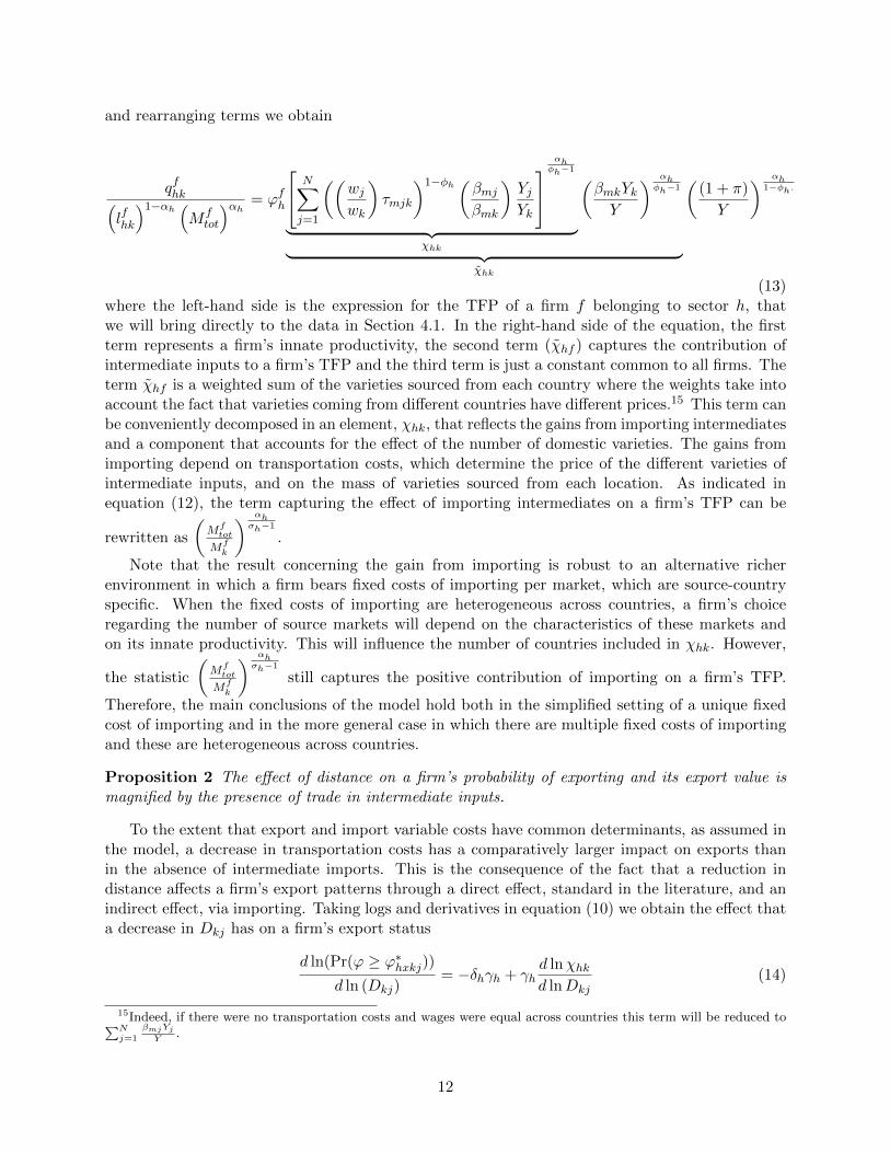
(13)where the left-hand side is the expression for the TFP of a firm f belonging to sector h, thatwe will bring directly to the data in Section 4.1. In the right-hand side of the equation, the firstterm represents a firm’s innate productivity, the second term (χhf ) captures the contribution ofintermediate inputs to a firm’s TFP and the third term is just a constant common to all firms. Theterm χhf is a weighted sum of the varieties sourced from each country where the weights take intoaccount the fact that varieties coming from different countries have different prices.15 This term canbe conveniently decomposed in an element, χhk, that reflects the gains from importing intermediatesand a component that accounts for the effect of the number of domestic varieties. The gains fromimporting depend on transportation costs, which determine the price of the different varieties ofintermediate inputs, and on the mass of varieties sourced from each location. As indicated inequation (12), the term capturing the effect of importing intermediates on a firm’s TFP can be

rewritten as

(Mftot

Mfk

) αhσh−1

.

Note that the result concerning the gain from importing is robust to an alternative richerenvironment in which a firm bears fixed costs of importing per market, which are source-countryspecific. When the fixed costs of importing are heterogeneous across countries, a firm’s choiceregarding the number of source markets will depend on the characteristics of these markets andon its innate productivity. This will influence the number of countries included in χhk. However,

the statistic

(Mftot

Mfk

) αhσh−1

still captures the positive contribution of importing on a firm’s TFP.

Therefore, the main conclusions of the model hold both in the simplified setting of a unique fixedcost of importing and in the more general case in which there are multiple fixed costs of importingand these are heterogeneous across countries.

Proposition 2 The effect of distance on a firm’s probability of exporting and its export value ismagnified by the presence of trade in intermediate inputs.

To the extent that export and import variable costs have common determinants, as assumed inthe model, a decrease in transportation costs has a comparatively larger impact on exports thanin the absence of intermediate imports. This is the consequence of the fact that a reduction indistance affects a firm’s export patterns through a direct effect, standard in the literature, and anindirect effect, via importing. Taking logs and derivatives in equation (10) we obtain the effect thata decrease in Dkj has on a firm’s export status

d ln(Pr(ϕ ≥ ϕ∗hxkj))d ln (Dkj)

= −δhγh + γhd lnχhkd lnDkj

(14)

15Indeed, if there were no transportation costs and wages were equal across countries this term will be reduced to∑Nj=1

βmjYjY

.

12

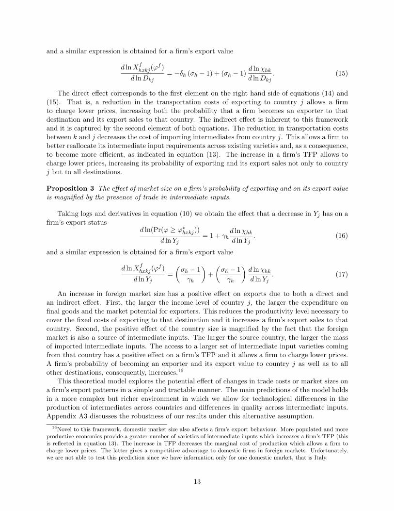
and a similar expression is obtained for a firm’s export value

d lnXfhxkj(ϕ

f )

d lnDkj= −δh (σh − 1) + (σh − 1)

d lnχhkd lnDkj

. (15)

The direct effect corresponds to the first element on the right hand side of equations (14) and(15). That is, a reduction in the transportation costs of exporting to country j allows a firmto charge lower prices, increasing both the probability that a firm becomes an exporter to thatdestination and its export sales to that country. The indirect effect is inherent to this frameworkand it is captured by the second element of both equations. The reduction in transportation costsbetween k and j decreases the cost of importing intermediates from country j. This allows a firm tobetter reallocate its intermediate input requirements across existing varieties and, as a consequence,to become more efficient, as indicated in equation (13). The increase in a firm’s TFP allows tocharge lower prices, increasing its probability of exporting and its export sales not only to countryj but to all destinations.

Proposition 3 The effect of market size on a firm’s probability of exporting and on its export valueis magnified by the presence of trade in intermediate inputs.

Taking logs and derivatives in equation (10) we obtain the effect that a decrease in Yj has on afirm’s export status

d ln(Pr(ϕ ≥ ϕ∗hxkj))d lnYj

= 1 + γhd lnχhkd lnYj

. (16)

and a similar expression is obtained for a firm’s export value

d lnXfhxkj(ϕ

f )

d lnYj=

(σh − 1

γh

)+

(σh − 1

γh

)d lnχhkd lnYj

. (17)

An increase in foreign market size has a positive effect on exports due to both a direct andan indirect effect. First, the larger the income level of country j, the larger the expenditure onfinal goods and the market potential for exporters. This reduces the productivity level necessary tocover the fixed costs of exporting to that destination and it increases a firm’s export sales to thatcountry. Second, the positive effect of the country size is magnified by the fact that the foreignmarket is also a source of intermediate inputs. The larger the source country, the larger the massof imported intermediate inputs. The access to a larger set of intermediate input varieties comingfrom that country has a positive effect on a firm’s TFP and it allows a firm to charge lower prices.A firm’s probability of becoming an exporter and its export value to country j as well as to allother destinations, consequently, increases.16

This theoretical model explores the potential effect of changes in trade costs or market sizes ona firm’s export patterns in a simple and tractable manner. The main predictions of the model holdsin a more complex but richer environment in which we allow for technological differences in theproduction of intermediates across countries and differences in quality across intermediate inputs.Appendix A3 discusses the robustness of our results under this alternative assumption.

16Novel to this framework, domestic market size also affects a firm’s export behaviour. More populated and moreproductive economies provide a greater number of varieties of intermediate inputs which increases a firm’s TFP (thisis reflected in equation 13). The increase in TFP decreases the marginal cost of production which allows a firm tocharge lower prices. The latter gives a competitive advantage to domestic firms in foreign markets. Unfortunately,we are not able to test this prediction since we have information only for one domestic market, that is Italy.

13

3 Data and Facts

Before turning to our empirical analysis, we describe the firm-level data and the country-levelvariables employed in the regressions.

3.1 Firm level data

The empirical analysis combines three sources of data collected by the Italian Statistical Office(ISTAT): the Italian Foreign Trade Statistics (COE), the Italian Register of Active Firms (ASIA)and a firm level accounting dataset (Micro 3).17

The COE dataset is the official source for the trade flows of Italy and it reports all cross-bordertransactions performed by Italian firms for the period 1998-2003. The database includes the value ofthe transactions, on a yearly basis, of a firm as disaggregated by countries of destination for exportsand markets of origin for imports.18 The total value of a firm-country transaction, recorded in euros,is broken down into five broad categories of goods, Main Industrial Groupings (MIGs), identifiedby EUROSTAT as energy, intermediate, capital, consumer durables and consumer non-durables.19

This is a unique feature of our dataset which allows distinguishing imported intermediate inputsfrom other types of imports.20

Using the unique identification code of a firm, we are able to link the trade data to ISTAT’sarchive of active firms, ASIA. The ASIA register covers the population of Italian firms active in thesame time span, irrespective of their trade status. It reports annual figures on number of employees,sector of main activity and information about the geographical location of the firms (municipalityof principal activity of legal address). The ASIA-COE dataset obtained by merging the two sourcesis not a sample but rather includes all active firms.

Data on firm-level characteristics come from Micro.3, which is a dataset based on the censusof Italian firms conducted yearly by ISTAT containing information on firms with more than 20employees covering all sectors of the economy for the period 1989-2007.21 Starting in 1998 thecensus of the whole population of firms only concerns companies with more than 100 employees,while in the range of employment 20-99, ISTAT directly monitors only a “rotating sample” whichvaries every five years. In order to complete the coverage of firms in that range, Micro.3 resorts, from1998 onward, to data from the financial statement that limited liability firms have to disclose, inaccordance to Italian law.22 The database contains information on a number of variables appearingin a firm’s balance sheet. For the purpose of this paper we use: number of employees, turnover,value added, capital, labour cost, intermediate inputs costs and capital assets. Capital is proxiedby tangible fixed assets at book value (net of depreciation). Nominal variables are in million eurosand are deflated using 2-digit industry-level production prices indices provided by ISTAT.

After merging these three databases, we work with an unbalanced panel of about 46,819 man-ufacturing firms over the sample period. Table 1 presents the number of firms active in the man-

17The database has been made available for work after careful screening to avoid disclosure of individual information.The data were accessed at the ISTAT facilities in Rome.

18ISTAT collects data on exports based on transactions. The European Union sets a common framework of rulesbut leaves some flexibility to member states. A detailed description of requirements for data collection on exportsand imports in Italy is provided in Appendix A4.

19EUROSTAT’s end-use categories (Main Industrial Groupings, MIGs), based on the Nace Rev. 2 classification,are defined by the Commission regulation (EC) n.656/2007 of 14 June 2007.

20Hereafter, when using the word “import” we refer to import of intermediate inputs unless otherwise specified.21The database has been built as a result of collaboration between ISTAT and a group of LEM researchers from

the Scuola Superiore Sant’Anna, Pisa. See Grazzi et al. (2013) for further details.22Limited liability companies (societa’ di capitali) have to provide a copy of their financial statement to the Register

of Firms at the local Chamber of Commerce.

14

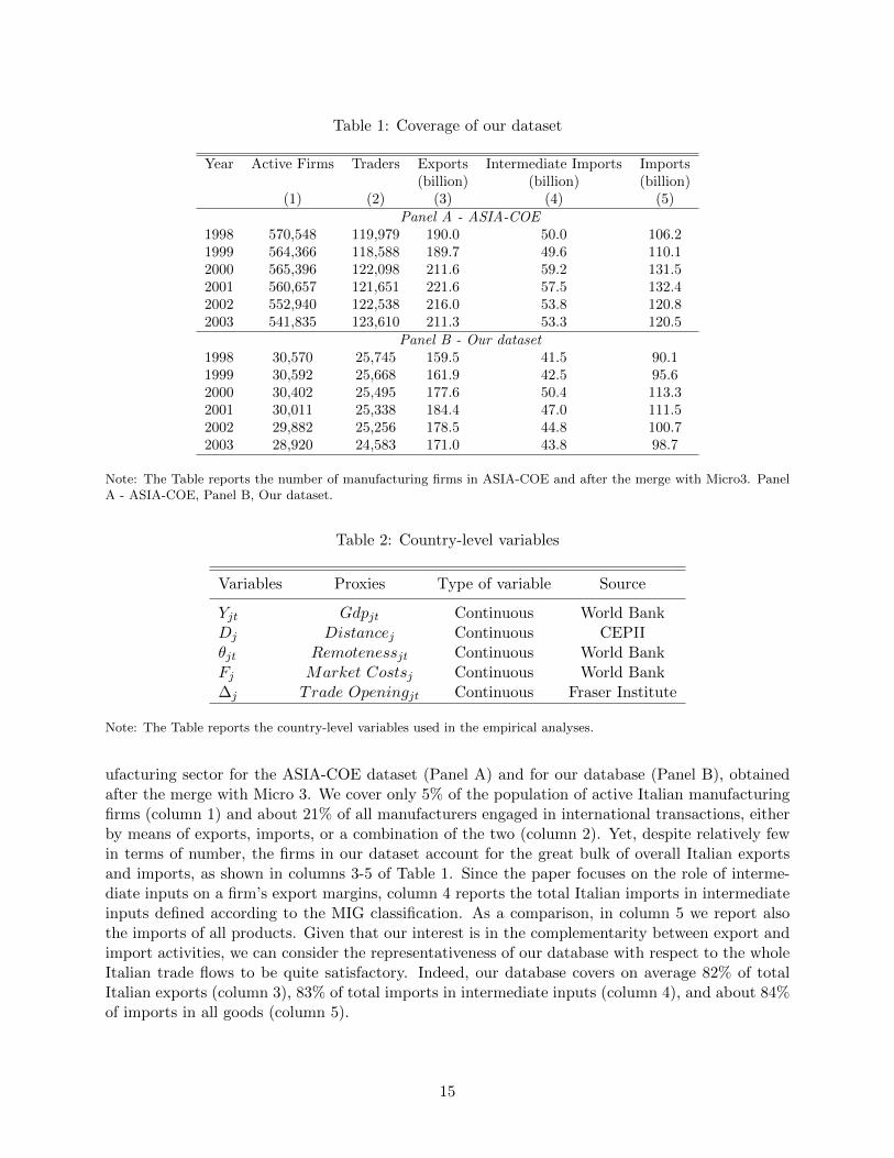
Table 1: Coverage of our dataset

Year Active Firms Traders Exports Intermediate Imports Imports(billion) (billion) (billion)

(1) (2) (3) (4) (5)Panel A - ASIA-COE

1998 570,548 119,979 190.0 50.0 106.21999 564,366 118,588 189.7 49.6 110.12000 565,396 122,098 211.6 59.2 131.52001 560,657 121,651 221.6 57.5 132.42002 552,940 122,538 216.0 53.8 120.82003 541,835 123,610 211.3 53.3 120.5

Panel B - Our dataset1998 30,570 25,745 159.5 41.5 90.11999 30,592 25,668 161.9 42.5 95.62000 30,402 25,495 177.6 50.4 113.32001 30,011 25,338 184.4 47.0 111.52002 29,882 25,256 178.5 44.8 100.72003 28,920 24,583 171.0 43.8 98.7

Note: The Table reports the number of manufacturing firms in ASIA-COE and after the merge with Micro3. PanelA - ASIA-COE, Panel B, Our dataset.

Table 2: Country-level variables

Variables Proxies Type of variable Source

Yjt Gdpjt Continuous World BankDj Distancej Continuous CEPIIθjt Remotenessjt Continuous World BankFj Market Costsj Continuous World Bank∆j Trade Openingjt Continuous Fraser Institute

Note: The Table reports the country-level variables used in the empirical analyses.

ufacturing sector for the ASIA-COE dataset (Panel A) and for our database (Panel B), obtainedafter the merge with Micro 3. We cover only 5% of the population of active Italian manufacturingfirms (column 1) and about 21% of all manufacturers engaged in international transactions, eitherby means of exports, imports, or a combination of the two (column 2). Yet, despite relatively fewin terms of number, the firms in our dataset account for the great bulk of overall Italian exportsand imports, as shown in columns 3-5 of Table 1. Since the paper focuses on the role of interme-diate inputs on a firm’s export margins, column 4 reports the total Italian imports in intermediateinputs defined according to the MIG classification. As a comparison, in column 5 we report alsothe imports of all products. Given that our interest is in the complementarity between export andimport activities, we can consider the representativeness of our database with respect to the wholeItalian trade flows to be quite satisfactory. Indeed, our database covers on average 82% of totalItalian exports (column 3), 83% of total imports in intermediate inputs (column 4), and about 84%of imports in all goods (column 5).

15

3.2 Country-level data

In addition to firm-level data, we complement the analysis with information on country character-istics. We consider the two standard gravity-type variables, GDPjt and Distancej to proxy formarket size (Yjt) and transportation costs (Dj), respectively. Data on GDP are taken from theWorld Bank’s World Development Indicators database. Information on geographical distance comesfrom CEPII. Distances are calculated following the great circle formula, which uses latitudes andlongitudes of the most important city (in terms of population) or of the official capital (De Sousaet al.; 2012).

We augment the gravity model by including additional variables that might be expected to affectthe costs of trading internationally. As predicted by equation (10) of our model, the probability ofexporting depends on variable trade costs not related to distance (∆j), market specific fixed costs(Fj) and a multilateral resistance term (θjt). At the same time equation (11) suggests that a firm’sexport sales to a specific destination can be modelled in a parallel fashion to the model for exportparticipation, though in this case market-specific fixed costs are not included.

For additional trade costs (∆j), we use a measure of average country-level import tariffs takenfrom the Fraser Institute (Trade Openingjt).

23 The market specific fixed costs (Fj) can be related tothe establishment of a foreign distribution network, difficulties in enforcing contractual agreements,or the uncertainty of dealing with foreign bureaucracies. Following Bernard et al. (2011), to generatea proxy for these costs we use information from three measures from the World Bank Doing Businessdataset: number of documents for importing, cost of importing and time to import (Djankov et al.;2010). Given the high level of correlation between these variables, we use the primary factor(Market Costsj) derived from principal component analysis as that factor accounts for most of thevariance contained in the original indicators. Finally, to proxy the multilateral resistance terms (θjt)we employ the variable Remotenessjt which captures the extent to which a country is separatedfrom other potential trade partners.24 The idea is that a remote country has high shipping costs,high import prices, and thus a high aggregate price index. As in Manova and Zhang (2012) thevariable remoteness is computed for each country as the distance weighted sum of the market sizesof all trading partners.25

Table 2 lists the country level characteristics used to proxy the variables in our empirical models.After selecting the destinations for which we have the information needed to carry out our analysis,we end up with a dataset including 109 countries.26

23This variable is a simple average of three sub-components: revenue from trade taxes, the mean tariff rate and thestandard deviation of tariffs. Each sub-component is a standardized measure ranging from 0 to 10 which is increasingin the freedom to trade internationally. For further details see J.Gwartney, R.Lawson and J.Hall, 2012, EconomicFreedom of the World - 2012 Annual Report, Fraser Institute.

24We are aware of the fact that the remoteness proxy bears little resemblance to its theoretical counterpart andthat a structural approach would be more adequate. However, in the empirical analyses our main interest lies in theelasticity of exports with respect to distance and market size. All the other country variables are simply included ascontrols.

25Precisely, Remotenessj =∑Nn=1 GDPn ∗ distancenj , where GDPn is the GDP of the origin country and

distancenj is the distance between n and j, and the summation is over all countries in the world n. An alternativemeasure of remoteness used in Baldwin and Harrigan (2011) is given by Remotenessj =

∑Nn=1(GDPn/distancenj)

−1.Our results are robust to the use of this other measure.

26The complete list of countries is reported in Table A1 in Appendix A5. Basic statistics for the different marketcharacteristics are reported in Table A2 in Appendix A5.

16

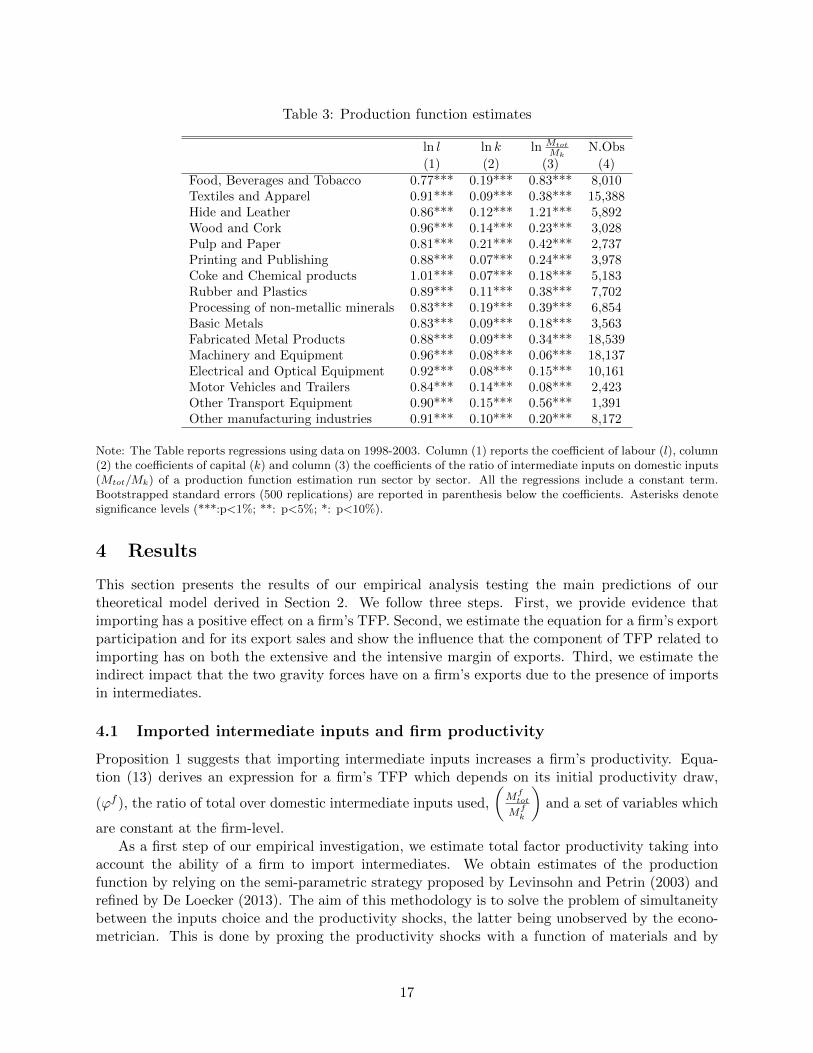
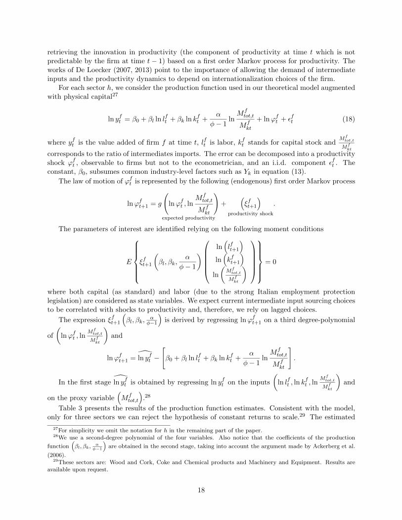
Table 3: Production function estimates

ln l ln k ln Mtot

MkN.Obs

(1) (2) (3) (4)Food, Beverages and Tobacco 0.77*** 0.19*** 0.83*** 8,010Textiles and Apparel 0.91*** 0.09*** 0.38*** 15,388Hide and Leather 0.86*** 0.12*** 1.21*** 5,892Wood and Cork 0.96*** 0.14*** 0.23*** 3,028Pulp and Paper 0.81*** 0.21*** 0.42*** 2,737Printing and Publishing 0.88*** 0.07*** 0.24*** 3,978Coke and Chemical products 1.01*** 0.07*** 0.18*** 5,183Rubber and Plastics 0.89*** 0.11*** 0.38*** 7,702Processing of non-metallic minerals 0.83*** 0.19*** 0.39*** 6,854Basic Metals 0.83*** 0.09*** 0.18*** 3,563Fabricated Metal Products 0.88*** 0.09*** 0.34*** 18,539Machinery and Equipment 0.96*** 0.08*** 0.06*** 18,137Electrical and Optical Equipment 0.92*** 0.08*** 0.15*** 10,161Motor Vehicles and Trailers 0.84*** 0.14*** 0.08*** 2,423Other Transport Equipment 0.90*** 0.15*** 0.56*** 1,391Other manufacturing industries 0.91*** 0.10*** 0.20*** 8,172

Note: The Table reports regressions using data on 1998-2003. Column (1) reports the coefficient of labour (l), column(2) the coefficients of capital (k) and column (3) the coefficients of the ratio of intermediate inputs on domestic inputs(Mtot/Mk) of a production function estimation run sector by sector. All the regressions include a constant term.Bootstrapped standard errors (500 replications) are reported in parenthesis below the coefficients. Asterisks denotesignificance levels (***:p<1%; **: p<5%; *: p<10%).

4 Results

This section presents the results of our empirical analysis testing the main predictions of ourtheoretical model derived in Section 2. We follow three steps. First, we provide evidence thatimporting has a positive effect on a firm’s TFP. Second, we estimate the equation for a firm’s exportparticipation and for its export sales and show the influence that the component of TFP related toimporting has on both the extensive and the intensive margin of exports. Third, we estimate theindirect impact that the two gravity forces have on a firm’s exports due to the presence of importsin intermediates.

4.1 Imported intermediate inputs and firm productivity

Proposition 1 suggests that importing intermediate inputs increases a firm’s productivity. Equa-tion (13) derives an expression for a firm’s TFP which depends on its initial productivity draw,

(ϕf ), the ratio of total over domestic intermediate inputs used,

(Mftot

Mfk

)and a set of variables which

are constant at the firm-level.As a first step of our empirical investigation, we estimate total factor productivity taking into

account the ability of a firm to import intermediates. We obtain estimates of the productionfunction by relying on the semi-parametric strategy proposed by Levinsohn and Petrin (2003) andrefined by De Loecker (2013). The aim of this methodology is to solve the problem of simultaneitybetween the inputs choice and the productivity shocks, the latter being unobserved by the econo-metrician. This is done by proxing the productivity shocks with a function of materials and by

17

retrieving the innovation in productivity (the component of productivity at time t which is notpredictable by the firm at time t− 1) based on a first order Markov process for productivity. Theworks of De Loecker (2007, 2013) point to the importance of allowing the demand of intermediateinputs and the productivity dynamics to depend on internationalization choices of the firm.

For each sector h, we consider the production function used in our theoretical model augmentedwith physical capital27

ln yft = β0 + βl ln lft + βk ln kft +

α

φ− 1lnMftot,t

Mfkt

+ lnϕft + εft (18)

where yft is the value added of firm f at time t, lft is labor, kft stands for capital stock andMftot,t

Mfkt

corresponds to the ratio of intermediates imports. The error can be decomposed into a productivityshock ϕft , observable to firms but not to the econometrician, and an i.i.d. component εft . Theconstant, β0, subsumes common industry-level factors such as Yk in equation (13).

The law of motion of ϕft is represented by the following (endogenous) first order Markov process

lnϕft+1 = g

(lnϕft , ln

Mftot,t

Mfkt

)expected productivity

+(ξft+1

)productivity shock

.

The parameters of interest are identified relying on the following moment conditions

E

ξft+1

(βl, βk,

α

φ− 1

)ln(lft+1

)ln(kft+1

)ln

(Mftot,t

Mfkt

) = 0

where both capital (as standard) and labor (due to the strong Italian employment protectionlegislation) are considered as state variables. We expect current intermediate input sourcing choicesto be correlated with shocks to productivity and, therefore, we rely on lagged choices.

The expression ξft+1

(βl, βk,

αφ−1

)is derived by regressing lnϕft+1 on a third degree-polynomial

of

(lnϕft , ln

Mftot,t

Mfkt

)and

lnϕft+1 = ln yft −

[β0 + βl ln l

ft + βk ln kft +

α

φ− 1lnMftot,t

Mfkt

].

In the first stage ln yft is obtained by regressing ln yft on the inputs

(ln lft , ln k

ft , ln

Mftot,t

Mfkt

)and

on the proxy variable(Mftot,t

).28

Table 3 presents the results of the production function estimates. Consistent with the model,only for three sectors we can reject the hypothesis of constant returns to scale.29 The estimated

27For simplicity we omit the notation for h in the remaining part of the paper.28We use a second-degree polynomial of the four variables. Also notice that the coefficients of the production

function(βl, βk,

αφ−1

)are obtained in the second stage, taking into account the argument made by Ackerberg et al.

(2006).29These sectors are: Wood and Cork, Coke and Chemical products and Machinery and Equipment. Results are

available upon request.

18

coefficients for the ratio of total over domestic intermediate inputs are always positive and statis-tically significant across different sectors, pointing to the importance of foreign intermediates inexplaining productivity differences across plants within sectors. At one extreme, for the Hide andLeather sector, we find that a 100% in the ratio of intermediate inputs on domestic inputs wouldincrease productivity by 121%. At the bottom of the sectoral distribution, this effect amounts to8% for the Motor Vehicles and Trailers sector.

4.2 The extensive and intensive margins of exports

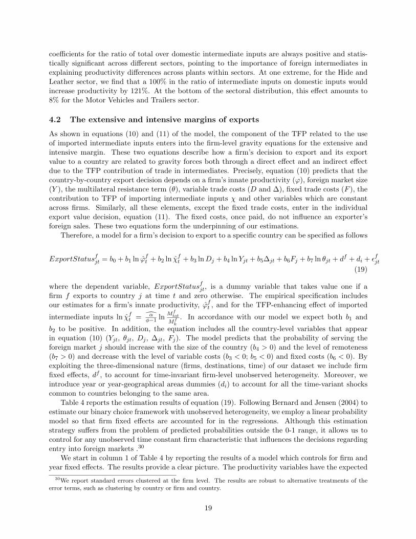
As shown in equations (10) and (11) of the model, the component of the TFP related to the useof imported intermediate inputs enters into the firm-level gravity equations for the extensive andintensive margin. These two equations describe how a firm’s decision to export and its exportvalue to a country are related to gravity forces both through a direct effect and an indirect effectdue to the TFP contribution of trade in intermediates. Precisely, equation (10) predicts that thecountry-by-country export decision depends on a firm’s innate productivity (ϕ), foreign market size(Y ), the multilateral resistance term (θ), variable trade costs (D and ∆), fixed trade costs (F ), thecontribution to TFP of importing intermediate inputs χ and other variables which are constantacross firms. Similarly, all these elements, except the fixed trade costs, enter in the individualexport value decision, equation (11). The fixed costs, once paid, do not influence an exporter’sforeign sales. These two equations form the underpinning of our estimations.

Therefore, a model for a firm’s decision to export to a specific country can be specified as follows

ExportStatusfjt = b0 + b1 ln ϕft + b2 ln χft + b3 lnDj + b4 lnYjt + b5∆jt + b6Fj + b7 ln θjt + df + di + εfjt(19)

where the dependent variable, ExportStatusfjt, is a dummy variable that takes value one if afirm f exports to country j at time t and zero otherwise. The empirical specification includesour estimates for a firm’s innate productivity, ϕft , and for the TFP-enhancing effect of imported

intermediate inputs ln χft = αφ−1 ln

Mftot

Mfk

. In accordance with our model we expect both b1 and

b2 to be positive. In addition, the equation includes all the country-level variables that appearin equation (10) (Yjt, θjt, Dj , ∆jt, Fj). The model predicts that the probability of serving theforeign market j should increase with the size of the country (b4 > 0) and the level of remoteness(b7 > 0) and decrease with the level of variable costs (b3 < 0; b5 < 0) and fixed costs (b6 < 0). Byexploiting the three-dimensional nature (firms, destinations, time) of our dataset we include firmfixed effects, df , to account for time-invariant firm-level unobserved heterogeneity. Moreover, weintroduce year or year-geographical areas dummies (di) to account for all the time-variant shockscommon to countries belonging to the same area.

Table 4 reports the estimation results of equation (19). Following Bernard and Jensen (2004) toestimate our binary choice framework with unobserved heterogeneity, we employ a linear probabilitymodel so that firm fixed effects are accounted for in the regressions. Although this estimationstrategy suffers from the problem of predicted probabilities outside the 0-1 range, it allows us tocontrol for any unobserved time constant firm characteristic that influences the decisions regardingentry into foreign markets .30

We start in column 1 of Table 4 by reporting the results of a model which controls for firm andyear fixed effects. The results provide a clear picture. The productivity variables have the expected

30We report standard errors clustered at the firm level. The results are robust to alternative treatments of theerror terms, such as clustering by country or firm and country.

19

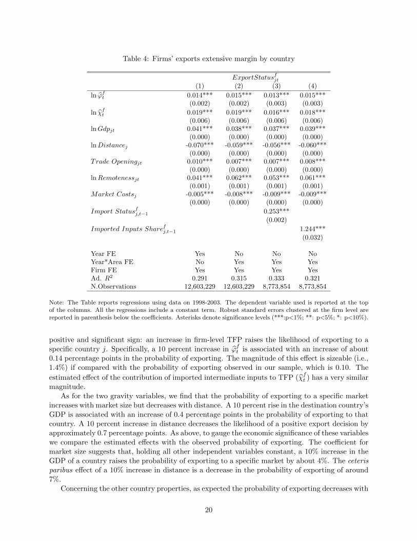
Table 4: Firms’ exports extensive margin by country

ExportStatusfjt(1) (2) (3) (4)

ln ϕft 0.014*** 0.015*** 0.013*** 0.015***

(0.002) (0.002) (0.003) (0.003)

ln χft 0.019*** 0.019*** 0.016*** 0.018***

(0.006) (0.006) (0.006) (0.006)lnGdpjt 0.041*** 0.038*** 0.037*** 0.039***

(0.000) (0.000) (0.000) (0.000)lnDistancej -0.070*** -0.059*** -0.056*** -0.060***

(0.000) (0.000) (0.000) (0.000)Trade Openingjt 0.010*** 0.007*** 0.007*** 0.008***

(0.000) (0.000) (0.000) (0.000)lnRemotenessjt 0.041*** 0.062*** 0.053*** 0.061***

(0.001) (0.001) (0.001) (0.001)Market Costsj -0.005*** -0.008*** -0.009*** -0.009***

(0.000) (0.000) (0.000) (0.000)

Import Statusfj,t−1 0.253***

(0.002)

Imported Inputs Sharefj,t−1 1.244***

(0.032)

Year FE Yes No No NoYear*Area FE No Yes Yes YesFirm FE Yes Yes Yes YesAd. R2 0.291 0.315 0.333 0.321N.Observations 12,603,229 12,603,229 8,773,854 8,773,854

Note: The Table reports regressions using data on 1998-2003. The dependent variable used is reported at the topof the columns. All the regressions include a constant term. Robust standard errors clustered at the firm level arereported in parenthesis below the coefficients. Asterisks denote significance levels (***:p<1%; **: p<5%; *: p<10%).

positive and significant sign: an increase in firm-level TFP raises the likelihood of exporting to aspecific country j. Specifically, a 10 percent increase in ϕft is associated with an increase of about0.14 percentage points in the probability of exporting. The magnitude of this effect is sizeable (i.e.,1.4%) if compared with the probability of exporting observed in our sample, which is 0.10. The

estimated effect of the contribution of imported intermediate inputs to TFP (χft ) has a very similarmagnitude.

As for the two gravity variables, we find that the probability of exporting to a specific marketincreases with market size but decreases with distance. A 10 percent rise in the destination country’sGDP is associated with an increase of 0.4 percentage points in the probability of exporting to thatcountry. A 10 percent increase in distance decreases the likelihood of a positive export decision byapproximately 0.7 percentage points. As above, to gauge the economic significance of these variableswe compare the estimated effects with the observed probability of exporting. The coefficient formarket size suggests that, holding all other independent variables constant, a 10% increase in theGDP of a country raises the probability of exporting to a specific market by about 4%. The ceterisparibus effect of a 10% increase in distance is a decrease in the probability of exporting of around7%.

Concerning the other country properties, as expected the probability of exporting decreases with

20

market costs. The negative and significant coefficient of Market Costs suggests the existence ofcountry-specific fixed export costs: the lower these costs are, the higher the probability of reaching amarket. Easy and accessible markets are likely to be served by a large number of firms, whereas lessaccessible countries with higher fixed export costs are more difficult to export to. The coefficientsfor Remoteness and Trade Opening have both the expected positive sign. Since remoteness makesa destination market less competitive, ceteris paribus, it is relatively easier for a firm to serve atrade partner that is geographically isolated from most other nations. The probability of exportingto a country should indeed increase with both the remoteness of the destination and its level offreedom to trade.

While in our initial specification we include firm and year fixed effects, it might be that thereare time-varying effects common to countries belonging to the same geographical area. Thus, incolumn 2 of Table 4 we replicate the previous regressions by including year-area fixed effects. Allthe results confirm the evidence from the specification with only year fixed effects.

In the baseline specification the effect of importing intermediate inputs comes only through χft .However, besides the TFP channel, there could be additional mechanisms through which importingintermediate inputs influences exporting. Indeed, one could imagine that importing from countryj reduces the fixed cost or the iceberg transport cost of exporting to country j. To account for thispossible effects we introduce in column 3 the (lagged) Import Status of a firm f from country jand in column 4 the (lagged) Imported Inputs Share of a firm f from country j, the latter definedas the ratio of a firm’s imports from j over the total value of intermediate inputs.

Our findings indicate that both the Import Status and the Imported Inputs Share enterwith a positive and significant coefficient, confirming the hypothesis that, after controlling for itsTFP effect, importing from a specific market has an additional positive effect on the probability ofexporting in that market. The coefficient for the Import Status variable implies that, conditional onχft , importing from country j has an effect which is more than two times the observed probabilityof exporting. Similarly, an increase of 1 percentage point in the import intensity from countryj is associated with an increase in the likelihood of a positive export decision of approximately0.012 points. Though these evidence points to the quantitative importance of non-TFP relatedmechanisms through which importing enhances exporting, the inclusion of these terms does notchange the sign or the magnitude of the other coefficients.31

Having established the determinants of a firm’s export participation across countries, we nextexplore whether firm and country differences are relevant for determining how much a firm sellsacross different markets, that is the intensive margin of exports. The econometric model, whichcan be thought of as a micro-gravity equation, takes the following form

lnExportsfjt = c0 + c1 ln ϕft + c2 ln χft + c3 lnDj + c4 lnYjt + c5∆jt + c6 ln θjt + df + di + εfjt (20)

where the dependent variable is the (log) total exports of firm f to country j at time t. As in theprevious equation, we include firm innate productivity, the TFP component related to the use ofimported inputs, country determinants, firm dummies and year (or year-area) dummies. Followingequation (11), we exclude the trade fixed costs variable.

The results are reported in Table 5. As for the export decision equation, we run the regres-sion controlling for year dummies (column 1) and then taking into account year-area fixed effects

31Using the contemporaneous values of Import Status and Imported Inputs Share do not alter the results. Ourfindings are robust also to controlling for the global import status (i.e., a dummy equal one if the firm imports fromat least one country).

21

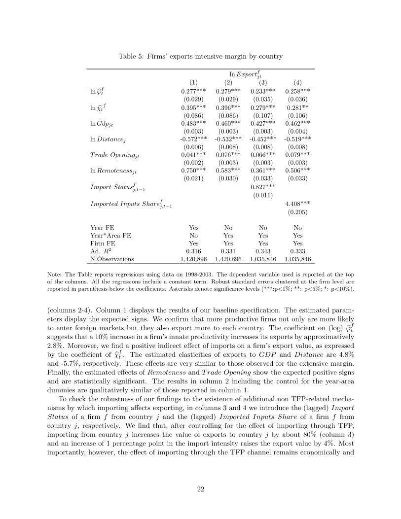
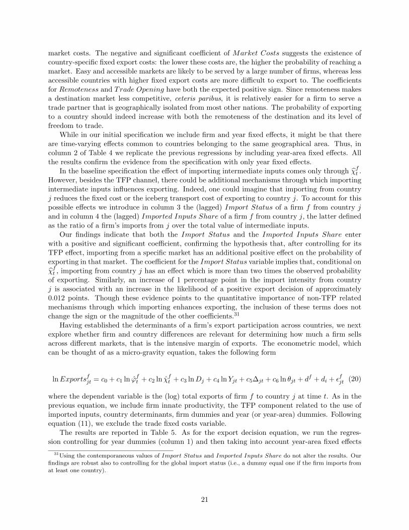
Table 5: Firms’ exports intensive margin by country

lnExportfjt(1) (2) (3) (4)

ln ϕft 0.277*** 0.279*** 0.233*** 0.258***

(0.029) (0.029) (0.035) (0.036)

ln χtf 0.395*** 0.396*** 0.279*** 0.281**

(0.086) (0.086) (0.107) (0.106)lnGdpjt 0.483*** 0.460*** 0.427*** 0.462***

(0.003) (0.003) (0.003) (0.004)lnDistancej -0.572*** -0.532*** -0.452*** -0.519***

(0.006) (0.008) (0.008) (0.008)Trade Openingjt 0.041*** 0.076*** 0.066*** 0.079***

(0.002) (0.003) (0.003) (0.003)lnRemotenessjt 0.750*** 0.583*** 0.361*** 0.506***

(0.021) (0.030) (0.033) (0.033)

Import Statusfj,t−1 0.827***

(0.011)

Imported Inputs Sharefj,t−1 4.408***

(0.205)

Year FE Yes No No NoYear*Area FE No Yes Yes YesFirm FE Yes Yes Yes YesAd. R2 0.316 0.331 0.343 0.333N.Observations 1,420,896 1,420,896 1,035,846 1,035,846

Note: The Table reports regressions using data on 1998-2003. The dependent variable used is reported at the topof the columns. All the regressions include a constant term. Robust standard errors clustered at the firm level arereported in parenthesis below the coefficients. Asterisks denote significance levels (***:p<1%; **: p<5%; *: p<10%).

(columns 2-4). Column 1 displays the results of our baseline specification. The estimated param-eters display the expected signs. We confirm that more productive firms not only are more likelyto enter foreign markets but they also export more to each country. The coefficient on (log) ϕftsuggests that a 10% increase in a firm’s innate productivity increases its exports by approximatively2.8%. Moreover, we find a positive indirect effect of imports on a firm’s export value, as expressedby the coefficient of χft . The estimated elasticities of exports to GDP and Distance are 4.8%and -5.7%, respectively. These effects are very similar to those observed for the extensive margin.Finally, the estimated effects of Remoteness and Trade Opening show the expected positive signsand are statistically significant. The results in column 2 including the control for the year-areadummies are qualitatively similar of those reported in column 1.

To check the robustness of our findings to the existence of additional non TFP-related mecha-nisms by which importing affects exporting, in columns 3 and 4 we introduce the (lagged) ImportStatus of a firm f from country j and the (lagged) Imported Inputs Share of a firm f fromcountry j, respectively. We find that, after controlling for the effect of importing through TFP,importing from country j increases the value of exports to country j by about 80% (column 3)and an increase of 1 percentage point in the import intensity raises the export value by 4%. Mostimportantly, however, the effect of importing through the TFP channel remains economically and

22

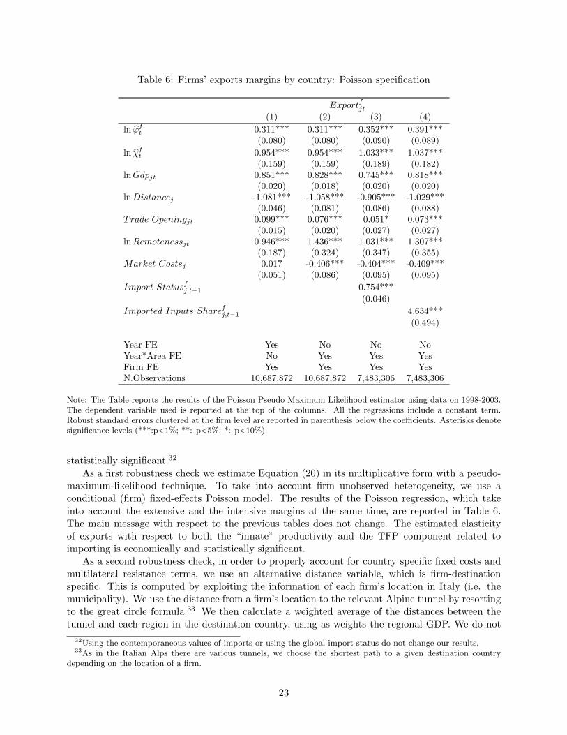
Table 6: Firms’ exports margins by country: Poisson specification

Exportfjt(1) (2) (3) (4)

ln ϕft 0.311*** 0.311*** 0.352*** 0.391***

(0.080) (0.080) (0.090) (0.089)

ln χft 0.954*** 0.954*** 1.033*** 1.037***

(0.159) (0.159) (0.189) (0.182)lnGdpjt 0.851*** 0.828*** 0.745*** 0.818***

(0.020) (0.018) (0.020) (0.020)lnDistancej -1.081*** -1.058*** -0.905*** -1.029***

(0.046) (0.081) (0.086) (0.088)Trade Openingjt 0.099*** 0.076*** 0.051* 0.073***

(0.015) (0.020) (0.027) (0.027)lnRemotenessjt 0.946*** 1.436*** 1.031*** 1.307***

(0.187) (0.324) (0.347) (0.355)Market Costsj 0.017 -0.406*** -0.404*** -0.409***

(0.051) (0.086) (0.095) (0.095)

Import Statusfj,t−1 0.754***

(0.046)

Imported Inputs Sharefj,t−1 4.634***

(0.494)

Year FE Yes No No NoYear*Area FE No Yes Yes YesFirm FE Yes Yes Yes YesN.Observations 10,687,872 10,687,872 7,483,306 7,483,306

Note: The Table reports the results of the Poisson Pseudo Maximum Likelihood estimator using data on 1998-2003.The dependent variable used is reported at the top of the columns. All the regressions include a constant term.Robust standard errors clustered at the firm level are reported in parenthesis below the coefficients. Asterisks denotesignificance levels (***:p<1%; **: p<5%; *: p<10%).

statistically significant.32

As a first robustness check we estimate Equation (20) in its multiplicative form with a pseudo-maximum-likelihood technique. To take into account firm unobserved heterogeneity, we use aconditional (firm) fixed-effects Poisson model. The results of the Poisson regression, which takeinto account the extensive and the intensive margins at the same time, are reported in Table 6.The main message with respect to the previous tables does not change. The estimated elasticityof exports with respect to both the “innate” productivity and the TFP component related toimporting is economically and statistically significant.

As a second robustness check, in order to properly account for country specific fixed costs andmultilateral resistance terms, we use an alternative distance variable, which is firm-destinationspecific. This is computed by exploiting the information of each firm’s location in Italy (i.e. themunicipality). We use the distance from a firm’s location to the relevant Alpine tunnel by resortingto the great circle formula.33 We then calculate a weighted average of the distances between thetunnel and each region in the destination country, using as weights the regional GDP. We do not

32Using the contemporaneous values of imports or using the global import status do not change our results.33As in the Italian Alps there are various tunnels, we choose the shortest path to a given destination country

depending on the location of a firm.

23

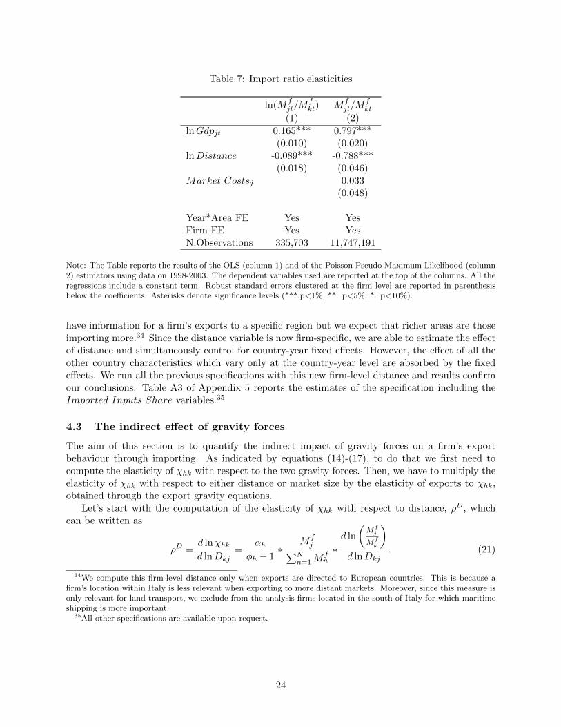
Table 7: Import ratio elasticities

ln(Mfjt/M

fkt) Mf

jt/Mfkt

(1) (2)

lnGdpjt 0.165*** 0.797***(0.010) (0.020)

lnDistance -0.089*** -0.788***(0.018) (0.046)

Market Costsj 0.033(0.048)

Year*Area FE Yes YesFirm FE Yes YesN.Observations 335,703 11,747,191

Note: The Table reports the results of the OLS (column 1) and of the Poisson Pseudo Maximum Likelihood (column2) estimators using data on 1998-2003. The dependent variables used are reported at the top of the columns. All theregressions include a constant term. Robust standard errors clustered at the firm level are reported in parenthesisbelow the coefficients. Asterisks denote significance levels (***:p<1%; **: p<5%; *: p<10%).

have information for a firm’s exports to a specific region but we expect that richer areas are thoseimporting more.34 Since the distance variable is now firm-specific, we are able to estimate the effectof distance and simultaneously control for country-year fixed effects. However, the effect of all theother country characteristics which vary only at the country-year level are absorbed by the fixedeffects. We run all the previous specifications with this new firm-level distance and results confirmour conclusions. Table A3 of Appendix 5 reports the estimates of the specification including theImported Inputs Share variables.35

4.3 The indirect effect of gravity forces

The aim of this section is to quantify the indirect impact of gravity forces on a firm’s exportbehaviour through importing. As indicated by equations (14)-(17), to do that we first need tocompute the elasticity of χhk with respect to the two gravity forces. Then, we have to multiply theelasticity of χhk with respect to either distance or market size by the elasticity of exports to χhk,obtained through the export gravity equations.

Let’s start with the computation of the elasticity of χhk with respect to distance, ρD, whichcan be written as

ρD =d lnχhkd lnDkj

=αh

φh − 1∗

Mfj∑N

n=1Mfn

∗d ln

(Mfj

Mfk

)d lnDkj

. (21)

34We compute this firm-level distance only when exports are directed to European countries. This is because afirm’s location within Italy is less relevant when exporting to more distant markets. Moreover, since this measure isonly relevant for land transport, we exclude from the analysis firms located in the south of Italy for which maritimeshipping is more important.

35All other specifications are available upon request.

24

Similarly, the elasticity of χhk with respect to market size, ρY , is given by

ρY =d lnχhkd lnYj

=αh

φh − 1∗

Mfj∑N

n=1Mfn

∗d ln

(Mfj

Mfk

)d lnYj

. (22)

The first term in both equations is the TFP elasticity to imports and can be retrieved by theestimates of the production function.36 The second element, which is directly observable in ourdata, is the fraction of imports of firm f from country j over the total intermediates inputs used bythe firm. The third term can be obtained by estimating the elasticity of the ratio of imports from jover domestic intermediates with respect to distance and GDP. According to our theoretical setting,the ratio of imports of intermediates from country j to domestic intermediates can be expressed by

Mfj

Mfk

=βmjYjβmkYk

((wjwk

)τmjk

)1−φ.

Given that the above expression is log-linear in distance and market size, we first estimate byOLS the following equation

lnMfjt

Mfkt

= a0 + a1 lnYjt + a2 lnDj + df + di + εfjt. (23)

where, in addition to the two gravity forces Y and D, we add a set of dummies to control forfirm-fixed effects df and for year-geographical areas, di. Then, to take into account the largeproportion of zeros observed in the data, we estimate the elasticity of the ratio with respect togravity forces by using a conditional (firm) fixed-effects Poisson regression. The estimates of thelog-linear specification are reported in column 1 of Table 7. In column 2 we show the results ofour preferred estimator, the Poisson regression, and we include as additional control the proxy forfixed costs Market Costs. We observe that the elasticity of the import ratio is slightly lower thanunity for both GDP and Distance. Therefore, it is confirmed that firms’ sourcing behaviour isinfluenced by the same standard gravity forces which are also active on the export side.37

With the three terms for the elasticity of χhk with respect to either distance or market size,we can now quantify the indirect effect of the two gravity forces on a firm’s export behavior bymultiplying ρD and ρY by the elasticity of exports to χhk, obtained in the gravity equation before.We consider the indirect effect of a generalized change in market size or transportation costs commonacross all countries. This is done by computing the second element of equations (21) and (22) asthe fraction of a firm’s imports from all countries over its total intermediates inputs. The resultsin Table 8 show the indirect effect of this generalized change using the elasticity of exports toχhk of the Poisson specification (see in Table 6). This allows us to quantify the indirect impact,considering together the extensive and the intensive margins of exports.38 Column 1 reports theindirect effect of GDP while column 2 the indirect effect of distance. The two columns report theaverage indirect impact by sector.

Our findings confirm that market size has a positive indirect effect on a firm’s export behaviourwhile distance a negative indirect impact. The results for distance are quantitatively very similar

36Colum 3 of Table 3.37In an unreported regression, where we use the firm-specific measure of distance together with year-country fixed

effects, we estimate an even greater elasticity to distance (i.e., 1.61).38In Table A4 of Appendix 5 we report the same calculations for the export extensive and intensive margins

separately. In Table A5 we also report the robustness check using the firm-specific distance variable. The results arequalitatively similar.

25

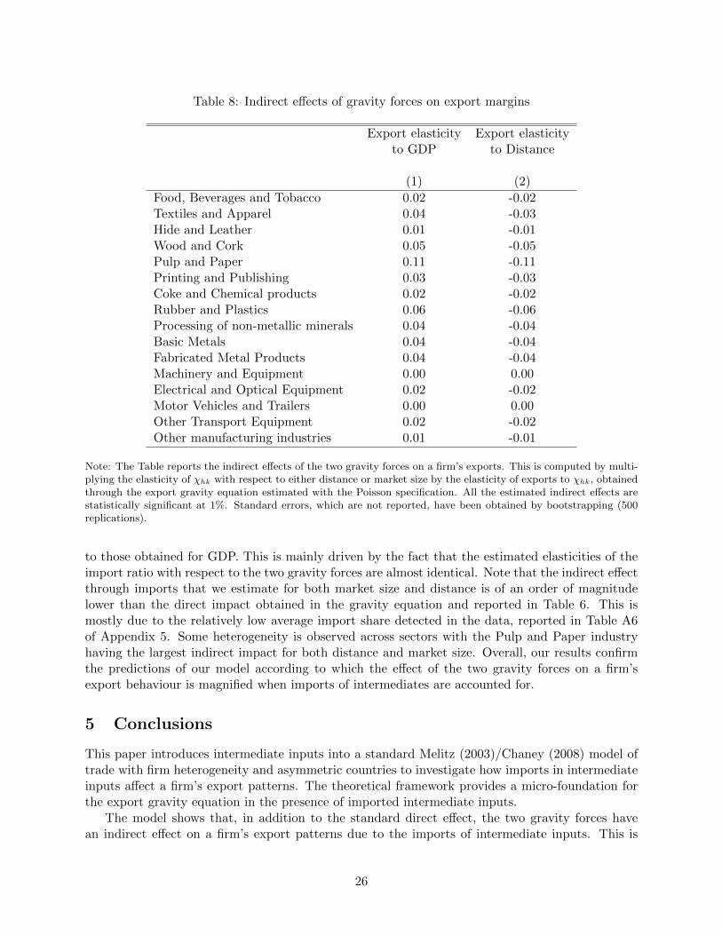
Table 8: Indirect effects of gravity forces on export margins

Export elasticity Export elasticityto GDP to Distance

(1) (2)

Food, Beverages and Tobacco 0.02 -0.02Textiles and Apparel 0.04 -0.03Hide and Leather 0.01 -0.01Wood and Cork 0.05 -0.05Pulp and Paper 0.11 -0.11Printing and Publishing 0.03 -0.03Coke and Chemical products 0.02 -0.02Rubber and Plastics 0.06 -0.06Processing of non-metallic minerals 0.04 -0.04Basic Metals 0.04 -0.04Fabricated Metal Products 0.04 -0.04Machinery and Equipment 0.00 0.00Electrical and Optical Equipment 0.02 -0.02Motor Vehicles and Trailers 0.00 0.00Other Transport Equipment 0.02 -0.02Other manufacturing industries 0.01 -0.01

Note: The Table reports the indirect effects of the two gravity forces on a firm’s exports. This is computed by multi-plying the elasticity of χhk with respect to either distance or market size by the elasticity of exports to χhk, obtainedthrough the export gravity equation estimated with the Poisson specification. All the estimated indirect effects arestatistically significant at 1%. Standard errors, which are not reported, have been obtained by bootstrapping (500replications).

to those obtained for GDP. This is mainly driven by the fact that the estimated elasticities of theimport ratio with respect to the two gravity forces are almost identical. Note that the indirect effectthrough imports that we estimate for both market size and distance is of an order of magnitudelower than the direct impact obtained in the gravity equation and reported in Table 6. This ismostly due to the relatively low average import share detected in the data, reported in Table A6of Appendix 5. Some heterogeneity is observed across sectors with the Pulp and Paper industryhaving the largest indirect impact for both distance and market size. Overall, our results confirmthe predictions of our model according to which the effect of the two gravity forces on a firm’sexport behaviour is magnified when imports of intermediates are accounted for.

5 Conclusions

This paper introduces intermediate inputs into a standard Melitz (2003)/Chaney (2008) model oftrade with firm heterogeneity and asymmetric countries to investigate how imports in intermediateinputs affect a firm’s export patterns. The theoretical framework provides a micro-foundation forthe export gravity equation in the presence of imported intermediate inputs.

The model shows that, in addition to the standard direct effect, the two gravity forces havean indirect effect on a firm’s export patterns due to the imports of intermediate inputs. This is

26

because importing has a positive effect on a firm’s productivity which depends on both the massof imported intermediate inputs available, as well as on the price of each intermediate. Therefore,an increase in foreign market size exerts a positive effect on exports directly but also indirectlythrough an efficiency increase induced by the imports of intermediate inputs. Similarly, a declinein transportation costs has an indirect effect on a firm’s exports pattern due to the reduction inthe cost of imported inputs which allows a firm to offer its exports at lower prices and to increaseits revenues in the exporting markets.

The propositions of the model are tested using a large and unique panel data set of Italianmanufacturing firms over the 1998-2003 period. Our empirical analysis confirm the predictions ofthe theoretical framework. First, by estimating a production function which takes into accountthe role of imported inputs, we show that imports contribute positively on a firm’s total factorproductivity. Second, we find that the component of productivity related to importing has apositive impact of on both margins of exports. Third, we quantify the indirect effects of the twogravity forces on a firm’s exports and confirm that the impact of market size and distance on afirm’s export behaviour is magnified when imports of intermediates are accounted for.

27

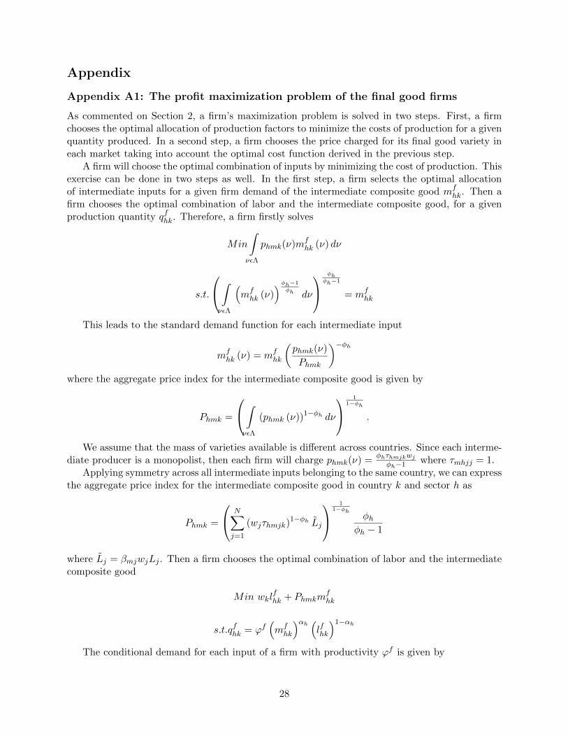
Appendix

Appendix A1: The profit maximization problem of the final good firms

As commented on Section 2, a firm’s maximization problem is solved in two steps. First, a firmchooses the optimal allocation of production factors to minimize the costs of production for a givenquantity produced. In a second step, a firm chooses the price charged for its final good variety ineach market taking into account the optimal cost function derived in the previous step.

A firm will choose the optimal combination of inputs by minimizing the cost of production. Thisexercise can be done in two steps as well. In the first step, a firm selects the optimal allocationof intermediate inputs for a given firm demand of the intermediate composite good mf

hk. Then afirm chooses the optimal combination of labor and the intermediate composite good, for a givenproduction quantity qfhk. Therefore, a firm firstly solves

Min

∫νεΛ

phmk(ν)mfhk (ν) dν

s.t.

∫νεΛ

(mfhk (ν)

)φh−1

φh dν

φhφh−1

= mfhk

This leads to the standard demand function for each intermediate input

mfhk (ν) = mf

hk

(phmk(ν)

Phmk

)−φhwhere the aggregate price index for the intermediate composite good is given by

Phmk =

∫νεΛ

(phmk (ν))1−φh dν

11−φh

.

We assume that the mass of varieties available is different across countries. Since each interme-diate producer is a monopolist, then each firm will charge phmk(ν) =

φhτhmjkwjφh−1 where τmhjj = 1.

Applying symmetry across all intermediate inputs belonging to the same country, we can expressthe aggregate price index for the intermediate composite good in country k and sector h as

Phmk =

N∑j=1

(wjτhmjk)1−φh Lj

11−φh

φhφh − 1

where Lj = βmjwjLj . Then a firm chooses the optimal combination of labor and the intermediatecomposite good

Min wklfhk + Phmkm

fhk

s.t.qfhk = ϕf(mfhk

)αh (lfhk

)1−αh

The conditional demand for each input of a firm with productivity ϕf is given by

28

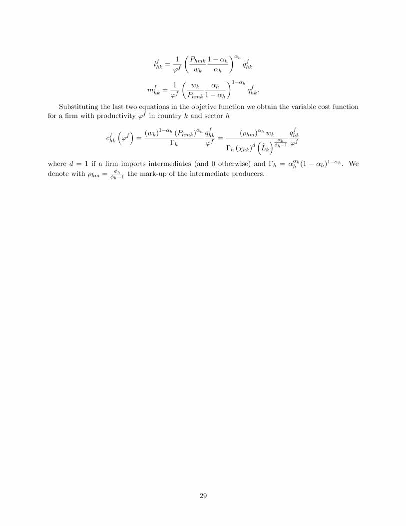
lfhk =1

ϕf

(Phmkwk

1− αhαh

)αhqfhk

mfhk =

1

ϕf

(wkPhmk

αh1− αh

)1−αhqfhk.

Substituting the last two equations in the objetive function we obtain the variable cost functionfor a firm with productivity ϕf in country k and sector h

cfhk

(ϕf)

=(wk)

1−αh (Phmk)αh

Γh

qfhkϕf

=(ρhm)αh wk

Γh (χhk)d(Lk

) αhφh−1

qfhkϕf

where d = 1 if a firm imports intermediates (and 0 otherwise) and Γh = ααhh (1 − αh)1−αh . We

denote with ρhm = φhφh−1 the mark-up of the intermediate producers.

29

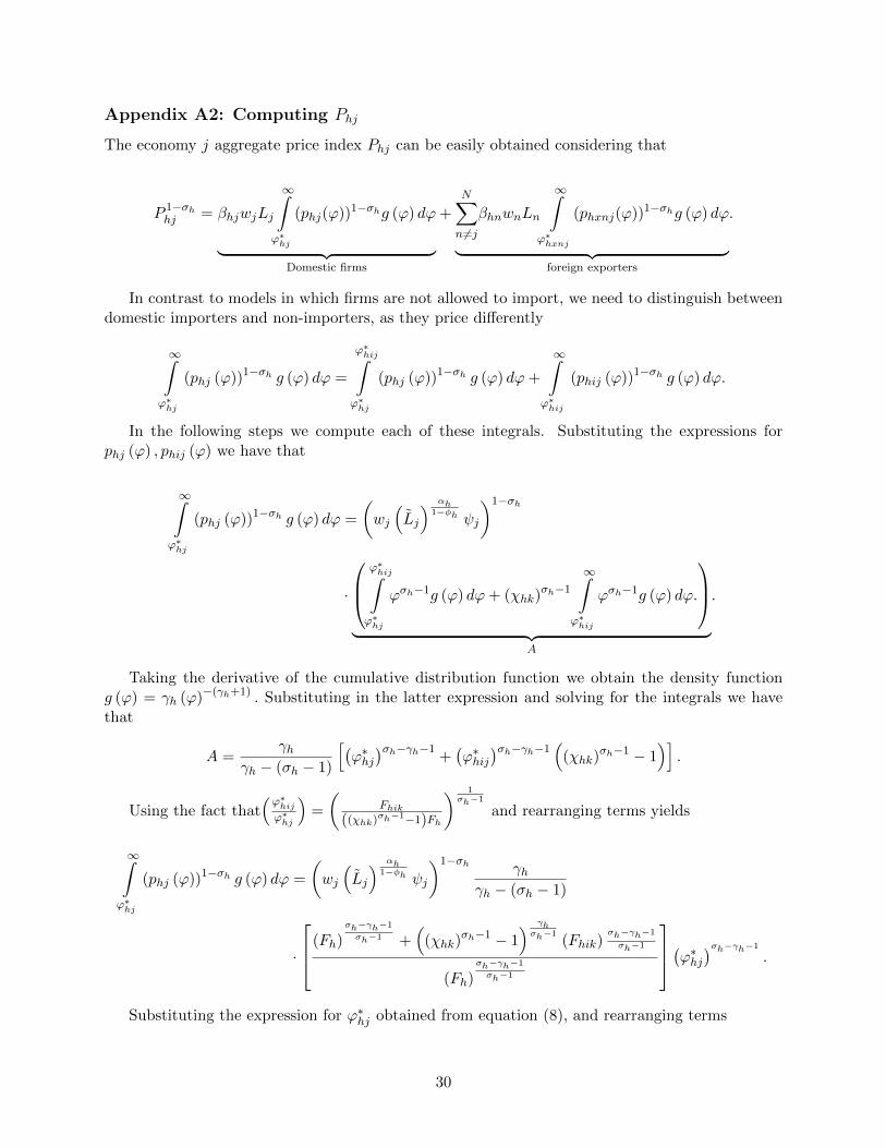
Appendix A2: Computing Phj

The economy j aggregate price index Phj can be easily obtained considering that

P 1−σhhj = βhjwjLj

∞∫ϕ∗hj

(phj(ϕ))1−σhg (ϕ) dϕ

︸ ︷︷ ︸Domestic firms

+

N∑n6=j

βhnwnLn

∞∫ϕ∗hxnj

(phxnj(ϕ))1−σhg (ϕ) dϕ

︸ ︷︷ ︸foreign exporters

.

In contrast to models in which firms are not allowed to import, we need to distinguish betweendomestic importers and non-importers, as they price differently

∞∫ϕ∗hj

(phj (ϕ))1−σh g (ϕ) dϕ =

ϕ∗hij∫ϕ∗hj

(phj (ϕ))1−σh g (ϕ) dϕ+

∞∫ϕ∗hij

(phij (ϕ))1−σh g (ϕ) dϕ.

In the following steps we compute each of these integrals. Substituting the expressions forphj (ϕ) , phij (ϕ) we have that

∞∫ϕ∗hj

(phj (ϕ))1−σh g (ϕ) dϕ =

(wj

(Lj

) αh1−φh ψj

)1−σh

·

ϕ∗hij∫ϕ∗hj

ϕσh−1g (ϕ) dϕ+ (χhk)σh−1

∞∫ϕ∗hij

ϕσh−1g (ϕ) dϕ.

︸ ︷︷ ︸

A

.

Taking the derivative of the cumulative distribution function we obtain the density functiong (ϕ) = γh (ϕ)−(γh+1) . Substituting in the latter expression and solving for the integrals we havethat

A =γh

γh − (σh − 1)

[(ϕ∗hj)σh−γh−1

+(ϕ∗hij

)σh−γh−1(

(χhk)σh−1 − 1

)].

Using the fact that(ϕ∗hijϕ∗hj

)=

(Fhik

((χhk)σh−1−1)Fh

) 1σh−1

and rearranging terms yields

∞∫ϕ∗hj

(phj (ϕ))1−σh g (ϕ) dϕ =

(wj

(Lj

) αh1−φh ψj

)1−σh γhγh − (σh − 1)

·

(Fh)σh−γh−1

σh−1 +(

(χhk)σh−1 − 1

) γhσh−1

(Fhik)σh−γh−1

σh−1

(Fh)σh−γh−1

σh−1

(ϕ∗hj)σh−γh−1

.

Substituting the expression for ϕ∗hj obtained from equation (8), and rearranging terms

30

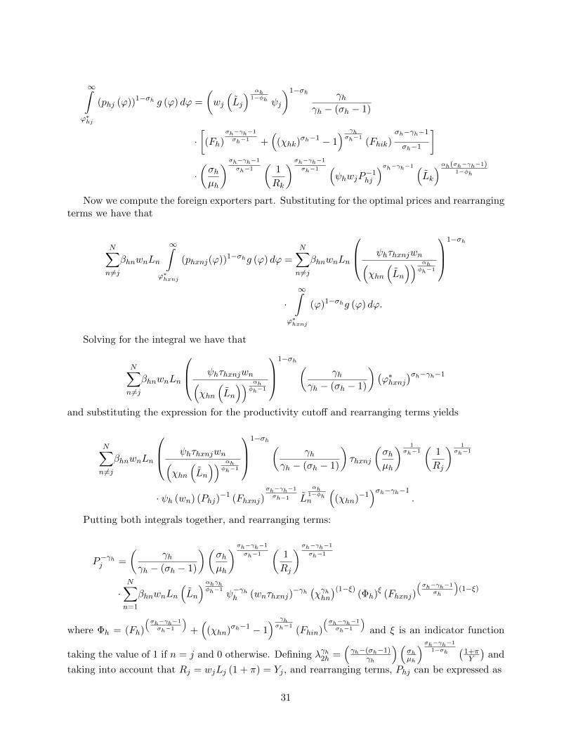
∞∫ϕ∗hj

(phj (ϕ))1−σh g (ϕ) dϕ =

(wj

(Lj

) αh1−φh ψj

)1−σh γhγh − (σh − 1)

·[(Fh)

σh−γh−1

σh−1 +(

(χhk)σh−1 − 1

) γhσh−1

(Fhik)σh−γh−1

σh−1

]

·(σhµh

)σh−γh−1

σh−1(

1

Rk

)σh−γh−1

σh−1 (ψhwjP

−1hj

)σh−γh−1 (Lk

)αh(σh−γh−1)1−φh

Now we compute the foreign exporters part. Substituting for the optimal prices and rearrangingterms we have that

N∑n 6=j

βhnwnLn

∞∫ϕ∗hxnj

(phxnj(ϕ))1−σhg (ϕ) dϕ =

N∑n 6=j

βhnwnLn

ψhτhxnjwn(χhn

(Ln

)) αhφh−1

1−σh

·∞∫

ϕ∗hxnj

(ϕ)1−σhg (ϕ) dϕ.

Solving for the integral we have that

N∑n6=j

βhnwnLn

ψhτhxnjwn(χhn

(Ln

)) αhφh−1

1−σh (

γhγh − (σh − 1)

)(ϕ∗hxnj

)σh−γh−1

and substituting the expression for the productivity cutoff and rearranging terms yields

N∑n 6=j

βhnwnLn

ψhτhxnjwn(χhn

(Ln

)) αhφh−1

1−σh (

γhγh − (σh − 1)

)τhxnj

(σhµh

) 1σh−1

(1

Rj

) 1σh−1

· ψh (wn) (Phj)−1 (Fhxnj)

σh−γh−1

σh−1 Lαh

1−φhn

((χhn)−1

)σh−γh−1.

Putting both integrals together, and rearranging terms:

P−γhj =

(γh

γh − (σh − 1)

)(σhµh

)σh−γh−1

σh−1(

1

Rj

)σh−γh−1

σh−1

·N∑n=1

βhnwnLn

(Ln

)αhγhφh−1

ψ−γhh (wnτhxnj)−γh (χγhhn)(1−ξ) (Φh)ξ (Fhxnj)

(σh−γh−1

σh

)(1−ξ)

where Φh = (Fh)

(σh−γh−1

σh−1

)+(

(χhn)σh−1 − 1) γhσh−1

(Fhin)

(σh−γh−1

σh−1

)and ξ is an indicator function

taking the value of 1 if n = j and 0 otherwise. Defining λγh2h =(γh−(σh−1)

γh

)(σhµh

)σh−γh−1

1−σh(

1+πY

)and

taking into account that Rj = wjLj (1 + π) = Yj , and rearranging terms, Phj can be expressed as

31

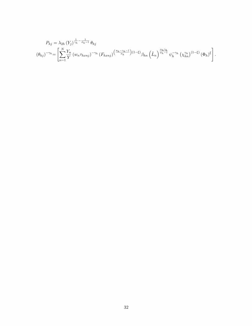
Phj = λ2h (Yj)1γh− 1σh−1 θhj

(θhj)−γh=

[N∑n=1

YnY

(wnτhxnj)−γh (Fhxnj)

(σh−γh−1

σh

)(1−ξ)

βhn

(Ln

)αhγhφh−1

ψ−γhh

(χγhhn

)(1−ξ)(Φh)ξ

].

32

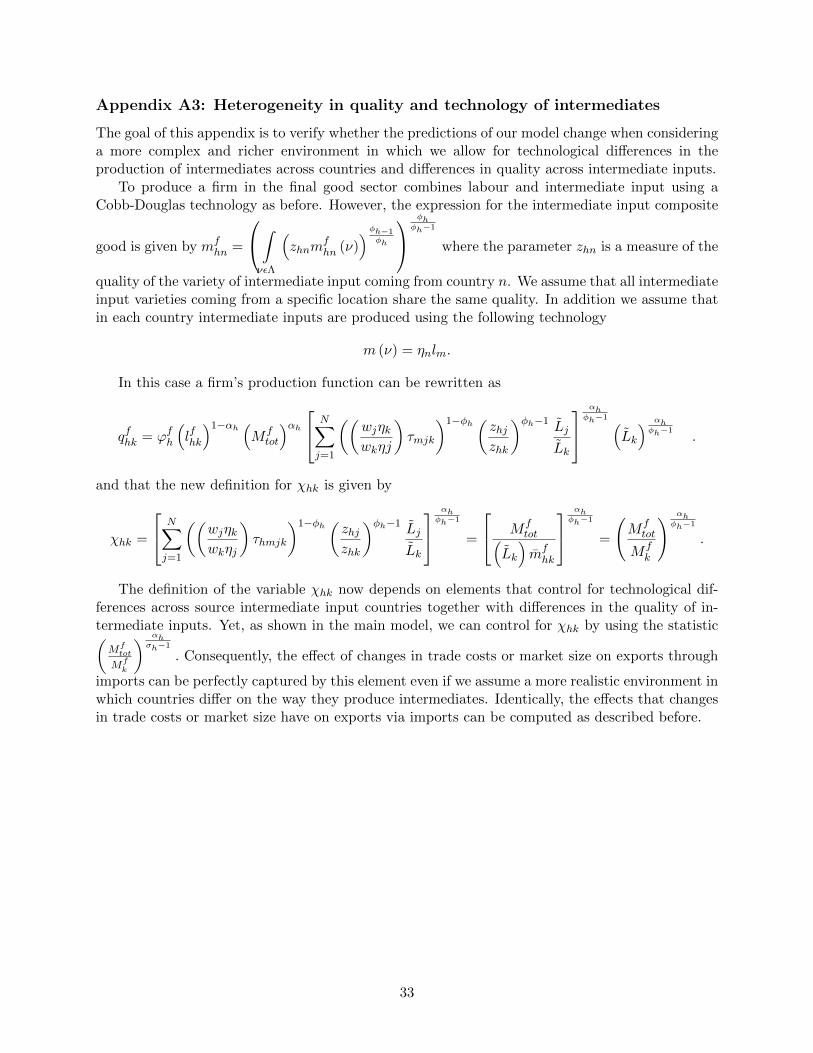
Appendix A3: Heterogeneity in quality and technology of intermediates

The goal of this appendix is to verify whether the predictions of our model change when consideringa more complex and richer environment in which we allow for technological differences in theproduction of intermediates across countries and differences in quality across intermediate inputs.

To produce a firm in the final good sector combines labour and intermediate input using aCobb-Douglas technology as before. However, the expression for the intermediate input composite

good is given by mfhn =

∫νεΛ

(zhnm

fhn (ν)

)φh−1φh

φhφh−1

where the parameter zhn is a measure of the

quality of the variety of intermediate input coming from country n. We assume that all intermediateinput varieties coming from a specific location share the same quality. In addition we assume thatin each country intermediate inputs are produced using the following technology

m (ν) = ηnlm.

In this case a firm’s production function can be rewritten as

qfhk = ϕfh

(lfhk

)1−αh (Mftot

)αh N∑j=1

((wjηkwkηj

)τmjk

)1−φh ( zhjzhk

)φh−1 Lj

Lk

αhφh−1 (

Lk

) αhφh−1

.

and that the new definition for χhk is given by

χhk =

N∑j=1

((wjηkwkηj

)τhmjk

)1−φh ( zhjzhk

)φh−1 Lj

Lk

αhφh−1

=

Mftot(

Lk

)mfhk

αhφh−1

=

(Mftot

Mfk

) αhφh−1

.

The definition of the variable χhk now depends on elements that control for technological dif-ferences across source intermediate input countries together with differences in the quality of in-termediate inputs. Yet, as shown in the main model, we can control for χhk by using the statistic(Mftot

Mfk

) αhσh−1

. Consequently, the effect of changes in trade costs or market size on exports through

imports can be perfectly captured by this element even if we assume a more realistic environment inwhich countries differ on the way they produce intermediates. Identically, the effects that changesin trade costs or market size have on exports via imports can be computed as described before.

33

Appendix A4: Custom data

In compliance with the common framework defined by the European Union (EU), there are differentrequirements in order for a transaction to be recorded, depending on whether the importing countryis an EU or NON-EU country, and on the value of the transaction.

As far as outside EU transactions are concerned, there is a good deal of homogeneity amongmember states as well as over time. In the Italian system the information is derived from the SingleAdministrative Document (SAD) which is compiled by operators for each individual transaction.Since the adoption of the Euro, Italy sets the threshold at 620 euro (or 1000 Kg), so that alltransactions bigger than 620 euro (or 1000 Kg) are recorded. For all of these recorded extra-EU transactions, the COE data report complete information, that is, also information about theproduct quantity and value.

Transactions within the EU are collected according to a different systems (Intrastat), where thethresholds on the annual value of transactions qualifying for a complete record are less homoge-neous across EU member states, with direct consequences on the type of information reported inthe data. In 2003 (the last year covered in the analysis), there are two cut-offs. If a firm has morethan 200,000 euro of exports (based on previous year report), then a firm must fill the Intrastat doc-ument monthly. This implies that complete information about product is also available. Instead, ifprevious year export value falls in between 40,000 and 200,000 euro, the quarterly Intrastat file hasto be filled, implying that only the amount of export is recorded, while information on the productis not. Firms with previous year exports below 40,000 euro are not required to report any infor-mation on trade flows. According to ISTAT, about one-third of the operators submitted monthlydeclarations, though covering about 98% of trade flows (http://www.coeweb.istat.it/default.htm).Thus, firms which do not appear in COE are either of this type (i.e. marginal exporters) or do notexport at all.

34

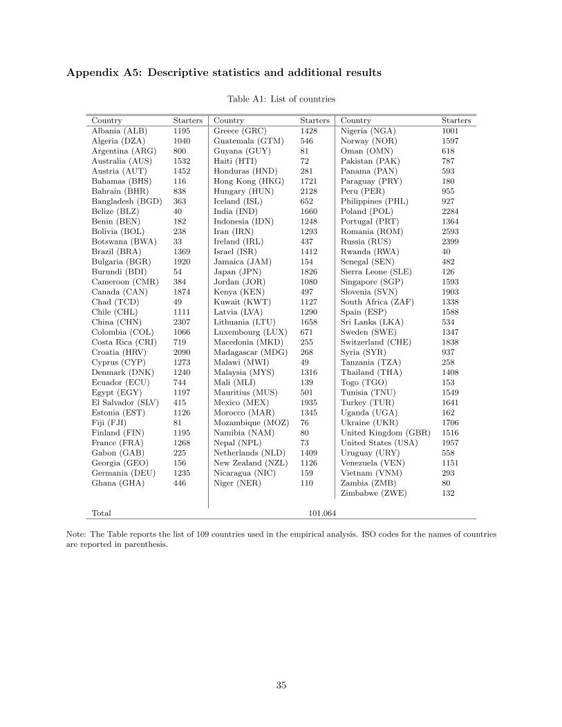
Appendix A5: Descriptive statistics and additional results

Table A1: List of countries

Country Starters Country Starters Country Starters

Albania (ALB) 1195 Greece (GRC) 1428 Nigeria (NGA) 1001Algeria (DZA) 1040 Guatemala (GTM) 546 Norway (NOR) 1597Argentina (ARG) 800 Guyana (GUY) 81 Oman (OMN) 618Australia (AUS) 1532 Haiti (HTI) 72 Pakistan (PAK) 787Austria (AUT) 1452 Honduras (HND) 281 Panama (PAN) 593Bahamas (BHS) 116 Hong Kong (HKG) 1721 Paraguay (PRY) 180Bahrain (BHR) 838 Hungary (HUN) 2128 Peru (PER) 955Bangladesh (BGD) 363 Iceland (ISL) 652 Philippines (PHL) 927Belize (BLZ) 40 India (IND) 1660 Poland (POL) 2284Benin (BEN) 182 Indonesia (IDN) 1248 Portugal (PRT) 1364Bolivia (BOL) 238 Iran (IRN) 1293 Romania (ROM) 2593Botswana (BWA) 33 Ireland (IRL) 437 Russia (RUS) 2399Brazil (BRA) 1369 Israel (ISR) 1412 Rwanda (RWA) 40Bulgaria (BGR) 1920 Jamaica (JAM) 154 Senegal (SEN) 482Burundi (BDI) 54 Japan (JPN) 1826 Sierra Leone (SLE) 126Cameroon (CMR) 384 Jordan (JOR) 1080 Singapore (SGP) 1593Canada (CAN) 1874 Kenya (KEN) 497 Slovenia (SVN) 1903Chad (TCD) 49 Kuwait (KWT) 1127 South Africa (ZAF) 1338Chile (CHL) 1111 Latvia (LVA) 1290 Spain (ESP) 1588China (CHN) 2307 Lithuania (LTU) 1658 Sri Lanka (LKA) 534Colombia (COL) 1066 Luxembourg (LUX) 671 Sweden (SWE) 1347Costa Rica (CRI) 719 Macedonia (MKD) 255 Switzerland (CHE) 1838Croatia (HRV) 2090 Madagascar (MDG) 268 Syria (SYR) 937Cyprus (CYP) 1273 Malawi (MWI) 49 Tanzania (TZA) 258Denmark (DNK) 1240 Malaysia (MYS) 1316 Thailand (THA) 1408Ecuador (ECU) 744 Mali (MLI) 139 Togo (TGO) 153Egypt (EGY) 1197 Mauritius (MUS) 501 Tunisia (TNU) 1549El Salvador (SLV) 415 Mexico (MEX) 1935 Turkey (TUR) 1641Estonia (EST) 1126 Morocco (MAR) 1345 Uganda (UGA) 162Fiji (FJI) 81 Mozambique (MOZ) 76 Ukraine (UKR) 1706Finland (FIN) 1195 Namibia (NAM) 80 United Kingdom (GBR) 1516France (FRA) 1268 Nepal (NPL) 73 United States (USA) 1957Gabon (GAB) 225 Netherlands (NLD) 1409 Uruguay (URY) 558Georgia (GEO) 156 New Zealand (NZL) 1126 Venezuela (VEN) 1151Germania (DEU) 1235 Nicaragua (NIC) 159 Vietnam (VNM) 293Ghana (GHA) 446 Niger (NER) 110 Zambia (ZMB) 80

Zimbabwe (ZWE) 132

Total 101,064

Note: The Table reports the list of 109 countries used in the empirical analysis. ISO codes for the names of countriesare reported in parenthesis.

35

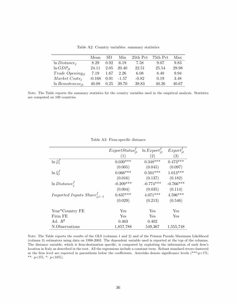
Table A2: Country variables: summary statistics

Mean SD Min 25th Pct 75th Pct Max

lnDistancej 8.29 0.92 6.19 7.58 9.07 9.83lnGDPjt 24.11 2.05 20.40 22.51 25.54 29.98Trade Openingjt 7.19 1.67 2.26 6.08 8.48 9.94Market Costsj -0.168 0.91 -1.57 -0.82 0.19 3.48lnRemotenessjt 40.08 0.25 39.70 39.83 40.26 40.67

Note: The Table reports the summary statistics for the country variables used in the empirical analysis. Statisticsare computed on 109 countries.

Table A3: Firm-specific distance

ExportStatusfjt lnExportfjt Exportfjt(1) (2) (3)

ln ϕft 0.030*** 0.348*** 0.473***(0.005) (0.045) (0.097)

ln χft 0.066*** 0.501*** 1.013***(0.016) (0.137) (0.182)

lnDistancefj -0.209*** -0.774*** -0.766***

(0.004) (0.035) (0.114)

Imported Inputs Sharefj,t−1 0.837*** 4.071*** 4.596***

(0.029) (0.213) (0.546)

Year*Country FE Yes Yes YesFirm FE Yes Yes YesAd. R2 0.463 0.402N.Observations 1,857,788 549,367 1,555,748

Note: The Table reports the results of the OLS (columns 1 and 2) and of the Poisson Pseudo Maximum Likelihood(column 3) estimators using data on 1998-2003. The dependent variable used is reported at the top of the columns.The distance variable, which is firm-destination specific, is computed by exploiting the information of each firm’slocation in Italy as described in the text. All the regressions include a constant term. Robust standard errors clusteredat the firm level are reported in parenthesis below the coefficients. Asterisks denote significance levels (***:p<1%;**: p<5%; *: p<10%).

36

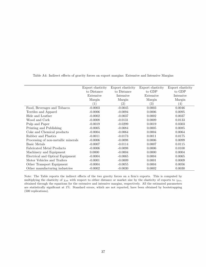
Table A4: Indirect effects of gravity forces on export margins: Extensive and Intensive Margins

Export elasticity Export elasticity Export elasticity Export elasticityto Distance to Distance to GDP to GDPExtensive Intensive Extensive IntensiveMargin Margin Margin Margin

(1) (2) (3) (4)Food, Beverages and Tobacco -0.0003 -0.0045 0.0003 0.0046Textiles and Apparel -0.0006 -0.0094 0.0006 0.0095Hide and Leather -0.0002 -0.0037 0.0002 0.0037Wood and Cork -0.0008 -0.0131 0.0009 0.0133Pulp and Paper -0.0019 -0.0299 0.0019 0.0303Printing and Publishing -0.0005 -0.0084 0.0005 0.0085Coke and Chemical products -0.0004 -0.0064 0.0004 0.0064Rubber and Plastics -0.0011 -0.0173 0.0011 0.0175Processing of non-metallic minerals -0.0006 -0.0098 0.0006 0.0099Basic Metals -0.0007 -0.0114 0.0007 0.0115Fabricated Metal Products -0.0006 -0.0098 0.0006 0.0100Machinery and Equipment 0.0000 -0.0004 0.0000 0.0004Electrical and Optical Equipment -0.0004 -0.0065 0.0004 0.0065Motor Vehicles and Trailers -0.0001 -0.0009 0.0001 0.0009Other Transport Equipment -0.0004 -0.0055 0.0004 0.0056Other manufacturing industries -0.0002 -0.0030 0.0002 0.0030

Note: The Table reports the indirect effects of the two gravity forces on a firm’s exports. This is computed bymultiplying the elasticity of χhk with respect to either distance or market size by the elasticity of exports to χhk,obtained through the equations for the extensive and intensive margins, respectively. All the estimated parametersare statistically significant at 1%. Standard errors, which are not reported, have been obtained by bootstrapping(500 replications).

37

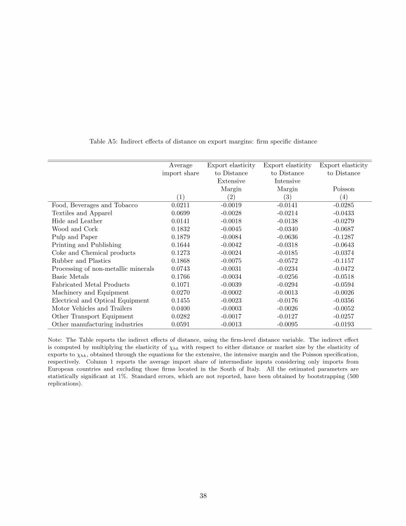
Table A5: Indirect effects of distance on export margins: firm specific distance

Average Export elasticity Export elasticity Export elasticityimport share to Distance to Distance to Distance

Extensive IntensiveMargin Margin Poisson

(1) (2) (3) (4)Food, Beverages and Tobacco 0.0211 -0.0019 -0.0141 -0.0285Textiles and Apparel 0.0699 -0.0028 -0.0214 -0.0433Hide and Leather 0.0141 -0.0018 -0.0138 -0.0279Wood and Cork 0.1832 -0.0045 -0.0340 -0.0687Pulp and Paper 0.1879 -0.0084 -0.0636 -0.1287Printing and Publishing 0.1644 -0.0042 -0.0318 -0.0643Coke and Chemical products 0.1273 -0.0024 -0.0185 -0.0374Rubber and Plastics 0.1868 -0.0075 -0.0572 -0.1157Processing of non-metallic minerals 0.0743 -0.0031 -0.0234 -0.0472Basic Metals 0.1766 -0.0034 -0.0256 -0.0518Fabricated Metal Products 0.1071 -0.0039 -0.0294 -0.0594Machinery and Equipment 0.0270 -0.0002 -0.0013 -0.0026Electrical and Optical Equipment 0.1455 -0.0023 -0.0176 -0.0356Motor Vehicles and Trailers 0.0400 -0.0003 -0.0026 -0.0052Other Transport Equipment 0.0282 -0.0017 -0.0127 -0.0257Other manufacturing industries 0.0591 -0.0013 -0.0095 -0.0193

Note: The Table reports the indirect effects of distance, using the firm-level distance variable. The indirect effectis computed by multiplying the elasticity of χhk with respect to either distance or market size by the elasticity ofexports to χhk, obtained through the equations for the extensive, the intensive margin and the Poisson specification,respectively. Column 1 reports the average import share of intermediate inputs considering only imports fromEuropean countries and excluding those firms located in the South of Italy. All the estimated parameters arestatistically significant at 1%. Standard errors, which are not reported, have been obtained by bootstrapping (500replications).

38

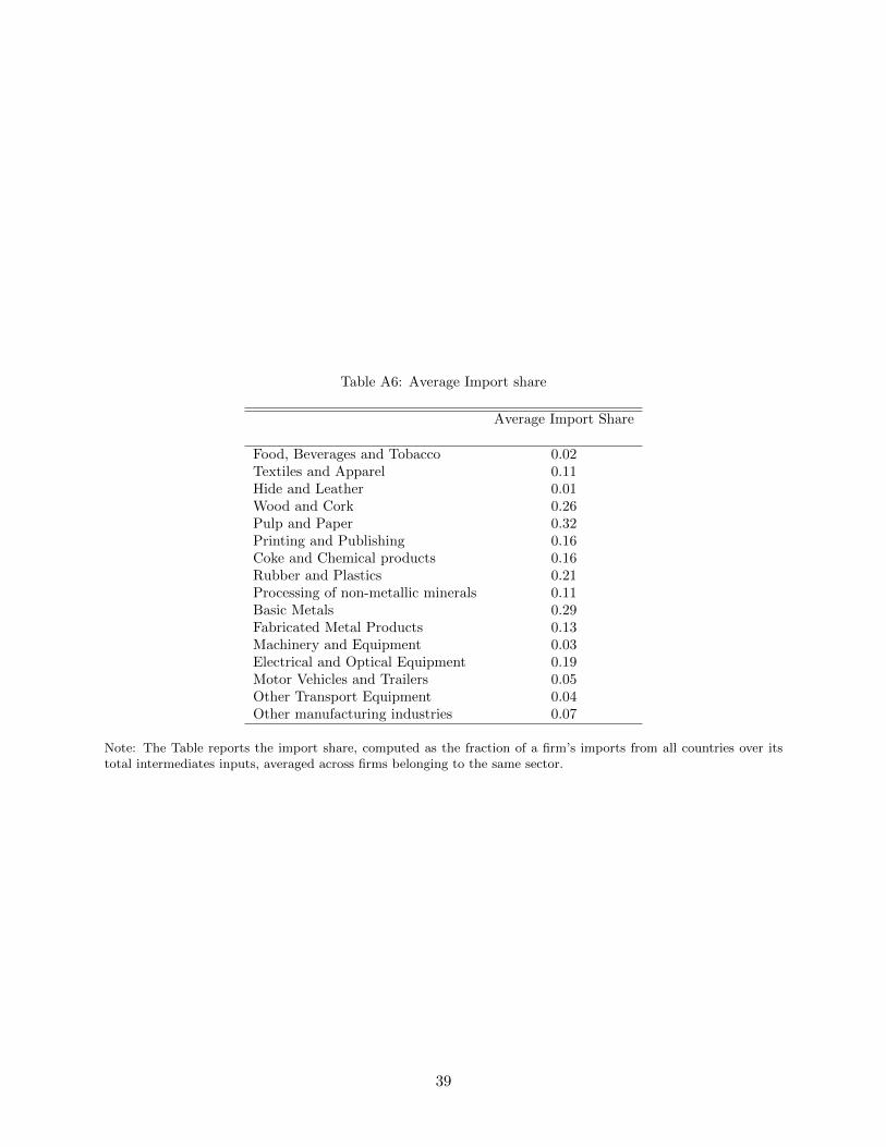
Table A6: Average Import share

Average Import Share

Food, Beverages and Tobacco 0.02Textiles and Apparel 0.11Hide and Leather 0.01Wood and Cork 0.26Pulp and Paper 0.32Printing and Publishing 0.16Coke and Chemical products 0.16Rubber and Plastics 0.21Processing of non-metallic minerals 0.11Basic Metals 0.29Fabricated Metal Products 0.13Machinery and Equipment 0.03Electrical and Optical Equipment 0.19Motor Vehicles and Trailers 0.05Other Transport Equipment 0.04Other manufacturing industries 0.07

Note: The Table reports the import share, computed as the fraction of a firm’s imports from all countries over itstotal intermediates inputs, averaged across firms belonging to the same sector.

39

References

Acharya, R. C. and Keller, W. (2009). Technology transfer through imports, Canadian Journal ofEconomics 42(4): 1411–1448.

Ackerberg, D., Caves, K. and Frazer, G. (2006). Structural identification of production functions,MPRA Paper 38349, University Library of Munich, Germany.

Aichele, R., Felbermayr, G. J. and Heiland, I. (2014). Going Deep: The Trade and Welfare Effectsof TTIP, CESifo Working Paper Series 5150, CESifo Group Munich.

Amiti, M. and Khandelwal, A. K. (2013). Import competition and quality upgrading, The Reviewof Economics and Statistics 95(2): 476–490.

Amiti, M. and Konings, J. (2007). Trade liberalization, intermediate inputs, and productivity:Evidence from indonesia, American Economic Review 97(5): 1611–1638.

Anderson, J. E. and van Wincoop, E. (2004). Trade costs, Journal of Economic Literature42(3): 691–751.

Baldwin, R. and Harrigan, J. (2011). Zeros, quality, and space: Trade theory and trade evidence,American Economic Journal: Microeconomics 3(2): 60–88.

Bas, M. and Strauss-Kahn, V. (2014). Does importing more inputs raise exports? firm levelevidence from france, Review of World Economics 150(2): 241–475.

Bernard, A. B., Grazzi, M. and Tomasi, C. (2011). Intermediaries in international trade: Directversus indirect modes of export, NBER Working Papers 17711, National Bureau of EconomicResearch, Inc.

Bernard, A. B. and Jensen, J. B. (2004). Why some firms export, The Review of Economics andStatistics 86(2): 561–569.

Bernard, A. B., Jensen, J. B., Redding, S. J. and Schott, P. K. (2007). Firms in international trade,Journal of Economic Perspectives 21(3): 105–130.

Caliendo, L. and Parro, F. (2015). Estimates of the Trade and Welfare Effects of NAFTA, Reviewof Economic Studies 82(1): 1–44.

Castellani, D., Serti, F. and Tomasi, C. (2010). Firms in international trade: Importers’ andexporters’ heterogeneity in italian manufacturing industry, The World Economy 33(3): 424–457.

Chaney, T. (2008). Distorted gravity: the intensive and extensive margins of international trade,American Economic Review 98(4): 1707–1721.

Crozet, M. and Koenig, P. (2010). Structural gravity equations with intensive and extensive mar-gins, Canadian Journal of Economics 43(1): 41–62.

De Loecker, J. (2007). Do exports generate higher productivity? evidence from slovenia, Journalof International Economics 73(1): 69–98.

De Loecker, J. (2013). Detecting Learning by Exporting, American Economic Journal: Microeco-nomics 5(3): 1–21.

40

De Sousa, J., Mayer, T. and Zignago, S. (2012). Market access in global and regional trade, RegionalScience and Urban Economics 42(6): 1037–1052.

Djankov, S., Freund, C. and Pham, C. S. (2010). Trading on time, Review of Economics andStatistics 92(1): 166–173.

Eaton, J., Kortum, S. and Kramarz, F. (2004). Dissecting trade: Firms, industries, and exportdestinations, American Economic Review 94(2): 150–154.

Eaton, J., Kortum, S. S. and Kramarz, F. (2011). An anatomy of international trade: Evidencefrom French firms, Econometrica 79(5): 1453–1498.

Feng, L., Li, Z. and Swenson, D. L. (2012). The connection between imported intermediate inputsand exports: Evidence from chinese firms, NBER Working Papers 18260, National Bureau ofEconomic Research, Inc.

Goldberg, P. K., Khandelwal, A. K., Pavcnik, N. and Topalova, P. (2010). Imported intermediateinputs and domestic product growth: Evidence from india, The Quarterly Journal of Economics125(4): 1727–1767.

Grazzi, M., Sanzo, R., Secchi, A. and Zeli, A. (2013). The building process of a new integratedsystem of business micro-data 1989-2004, Journal of Economic and Social Measurement (4): 291–324.

Grossman, G. M. and Helpman, E. (1991). Innovation and Growth in the Global Economy, Cam-bridge, Mass. ; London : MIT.

Halpern, L., Koren, M. and Szeidl, A. (2011). Imported inputs and productivity, CeFiG WorkingPapers 8, Center for Firms in the Global Economy.

Helpman, E., Melitz, M. and Rubinstein, Y. (2008). Estimating trade flows: Trading partners andtrading volumes, The Quarterly Journal of Economics 123(2): 441–487.

Hummels, D., Ishii, J. and Yi, K.-M. (2001). The nature and growth of vertical specialization inworld trade, Journal of International Economics 54(1): 75–96.

Kasahara, H. and Lapham, B. (2013). Productivity and the decision to import and export: Theoryand evidence, Journal of International Economics 89(2): 297–316.

Kasahara, H. and Rodrigue, J. (2008). Does the use of imported intermediates increase productiv-ity? plant-level evidence, Journal of Development Economics 87(1): 106–118.

Lawless, M. and Whelan, K. (2008). Where do firms export, how much, and why?, Working Papers200821, School Of Economics, University College Dublin.

Levinsohn, J. and Petrin, A. (2003). Estimating production functions using inputs to control forunobservables, Review of Economic Studies 70(2): 317–41.

Manova, K. and Zhang, Z. (2012). Export prices across firms and destinations, The QuarterlyJournal of Economics 127(1): 379–436.

Markusen, J. (1989). Trade in producer services and in other specialized intermediate inputs,American Economic Review 79(1): 85–95.

41

Mayer, T. and Ottaviano, G. (2008). The happy few: The internationalisation of european firms,Intereconomics: Review of European Economic Policy 43(3): 135–148.

Melitz, M. J. (2003). The impact of trade on intra-industry reallocations and aggregate industryproductivity, Econometrica 71(6): 1695–1725.

Muuls, M. and Pisu, M. (2009). Imports and exports at the level of the firm: Evidence frombelgium, The World Economy 32(5): 692–734.

Nocco, A. (2012). Selection, market size and international integration: Do vertical linkages play arole?, Review of International Economics 20(5): 960–973.

Rivera-Batiz, L. A. and Romer, P. M. (1991). International trade with endogenous technologicalchange, European Economic Review 35(4): 971–1001.

Romer, P. M. (1990). Endogenous technological change, Journal of Political Economy 98(5): S71–102.

Smeets, R., Creusen, H., Lejour, A. and Kox, H. (2010). Export margins and export barriers: Un-covering market entry costs of exporters in the netherlands, CPB Documents 208, CPB Nether-lands Bureau for Economic Policy Analysis.

Tinbergen, J. (1962). Shaping the World Economy: sugggestions for an International EconomicPolicy, Twentieth Century Fund, New-York.

Yi, K.-M. (2003). Can vertical specialization explain the growth of world trade?, Journal of PoliticalEconomy 111(1): 52–102.

42