Misallocation or Mismeasurement? by University of ...
41
Misallocation or Mismeasurement? by Mark Bils University of Rochester and NBER Peter J. Klenow Stanford University and NBER Cian Ruane International Monetary Fund CES 20-07 February, 2020 The research program of the Center for Economic Studies (CES) produces a wide range of economic analyses to improve the statistical programs of the U.S. Census Bureau. Many of these analyses take the form of CES research papers. The papers have not undergone the review accorded Census Bureau publications and no endorsement should be inferred. Any opinions and conclusions expressed herein are those of the author(s) and do not necessarily represent the views of the U.S. Census Bureau. All results have been reviewed to ensure that no confidential information is disclosed. Republication in whole or part must be cleared with the authors. To obtain information about the series, see www.census.gov/ces or contact Christopher Goetz, Editor, Discussion Papers, U.S. Census Bureau, Center for Economic Studies 5K038E, 4600 Silver Hill Road, Washington, DC 20233, [email protected]. To subscribe to the series, please click here.
Transcript of Misallocation or Mismeasurement? by University of ...
Misallocation or Mismeasurement?
by
Mark Bils University of Rochester and NBER
Peter J. Klenow Stanford University and NBER
Cian Ruane International Monetary Fund
CES 20-07 February, 2020
The research program of the Center for Economic Studies (CES) produces a wide range of economic analyses to improve the statistical programs of the U.S. Census Bureau. Many of these analyses take the form of CES research papers. The papers have not undergone the review accorded Census Bureau publications and no endorsement should be inferred. Any opinions and conclusions expressed herein are those of the author(s) and do not necessarily represent the views of the U.S. Census Bureau. All results have been reviewed to ensure that no confidential information is disclosed. Republication in whole or part must be cleared with the authors.
To obtain information about the series, see www.census.gov/ces or contact Christopher Goetz, Editor, Discussion Papers, U.S. Census Bureau, Center for Economic Studies 5K038E, 4600 Silver Hill Road, Washington, DC 20233, [email protected]. To subscribe to the series, please click here.

Abstract
The ratio of revenue to inputs differs greatly across plants within countries such as the U.S. and India. Such gaps may reflect misallocation which hinders aggregate productivity. But differences in measured average products need not reflect differences in true marginal products. We propose a way to estimate the gaps in true marginal products in the presence of measurement error. Our method exploits how revenue growth is less sensitive to input growth when a plant’s average products are overstated by measurement error. For Indian manufacturing from 1985–2013, our correction lowers potential gains from reallocation by 20%. For the U.S. the effect is even more dramatic, reducing potential gains by 60% and eliminating 2/3 of a severe downward trend in allocative efficiency over 1978–2013. *
* We are grateful to seminar participants and, especially, Joel David for comments. Any opinions and conclusions expressed herein are those of the author(s) and do not necessarily represent the views of the U.S. Census Bureau, the IMF, its Executive Board, or its management.. This research was performed at a Federal Statistical Research Data Center under FSRDC Project 1440. All results have been reviewed to ensure that no confidential information is disclosed.

2 BILS, KLENOW, AND RUANE
1. Introduction
The ratio of revenue to inputs differs substantially across establishments within
narrow industries in the U.S. and other countries. See the survey by Syverson
(2011). One interpretation of such gaps is that they reflect differences in the
value of marginal products for capital, labor, and intermediate inputs. Such
differences may imply misallocation, with negative consequences for aggre-
gate productivity. This point has been driven home by Restuccia and Rogerson
(2008) and Hsieh and Klenow (2009). See Hopenhayn (2014) and Restuccia and
Rogerson (2017) for surveys of the growing literature surrounding this topic.
Differences in measured average products need not imply differences in true
marginal products. First, marginal products are proportional to average prod-
ucts only under Cobb-Douglas production. Second, and to our point of em-
phasis, measured differences in revenue per inputs could simply reflect poor
measurement of revenue or costs. For example, the capital stock is typically a
book value measure that need not closely reflect the market value of physical
capital. Misstatement of inventories will contaminate and distort measures of
gross output and intermediates, since these are inferred in part based on the
change in finished, work in process, and materials inventories.1
We propose and implement a method to quantify the extent to which mea-
sured average products reflect true marginal products in the presence of mea-
surement error and overhead costs. Our method is able to detect measurement
error in revenue and inputs which is additive but whose variance can scale up
with the plant’s true revenue and inputs. Our method cannot identify pro-
portional measurement error, and therefore may yield a lower bound on the
magnitude of measurement error.
1See White, Reiter and Petrin (2018) for how the U.S. Census Bureau tries to correct formeasurement errors in its survey data on manufacturing plants. Rotemberg and White (2019)argue that the use of imputation in the U.S. but (perhaps) not in India could account forwhy allocative efficiency seems higher in the U.S. than in India. Bartelsman, Haltiwangerand Scarpetta (2013) and Asker, Collard-Wexler and De Loecker (2014) discuss why revenueproductivity need not reflect misallocation even aside from measurement error, due tooverhead costs and adjustment costs, respectively.

MISALLOCATION OR MISMEASUREMENT? 3
The intuition for our method is as follows. Imagine a world with constant
(proportional) differences in true marginal products. The only shocks are to
idiosyncratic plant productivity. Productivity shocks will move true revenue
and inputs around across plants in the same proportion.2 Thus, in the absence
of measurement error, revenue growth will be proportional to input growth
across all plants. Now suppose, instead, that revenue is overstated for a given
plant. If this measurement error is additive and fixed over time, then the plant’s
measured revenue will move by less in percentage terms in response to a change
in its productivity. Similarly, if a plant has overstated inputs in an additive
and fixed way, its measured inputs will move less than proportionately in re-
sponse to productivity shocks. Thus, if a plants revenue/inputs are overstated
by measurement error, its measured revenue growth will be less responsive to
its measured input growth. We can then gauge the importance of measurement
error in the cross-section by the degree to which high average product plants
exhibit a low elasticity of revenue with respect to inputs over time.
Our method applies to less stark environments with changing true marginal
products and measurement error over time for plants. A key restriction we
do require is that the measurement errors be orthogonal to the true marginal
products. As we will show, our approach involves regressing revenue growth
on input growth within each decile of average products. The extent to which
the resulting coefficients decrease with the decile (level) of TFPR speak to how
much measurement error is contributing to the dispersion in measured average
products in the cross-section.
We apply our methodology to panel data on U.S. manufacturing plants from
1978–2013 and formal Indian manufacturing plants from 1985–2013. The U.S.
data is from the Annual Survey of Manufacturers (ASM) plus ASM plants in
Census years, both from the Longitudinal Research Database (LRD). The Indian
data is from the Annual Survey of Industries (ASI). The LRD contains about
2Output increases more than inputs in response to a productivity shock, of course. But aplant’s relative output price will decline with productivity so that its revenue will rise by the sameproportion as its inputs. This is true if the plant’s price-cost markup, or true ratio of revenue toinputs, does not change with its productivity.

4 BILS, KLENOW, AND RUANE
50,000 ASM plants per year, and the ASI about 43,000 plants per year.
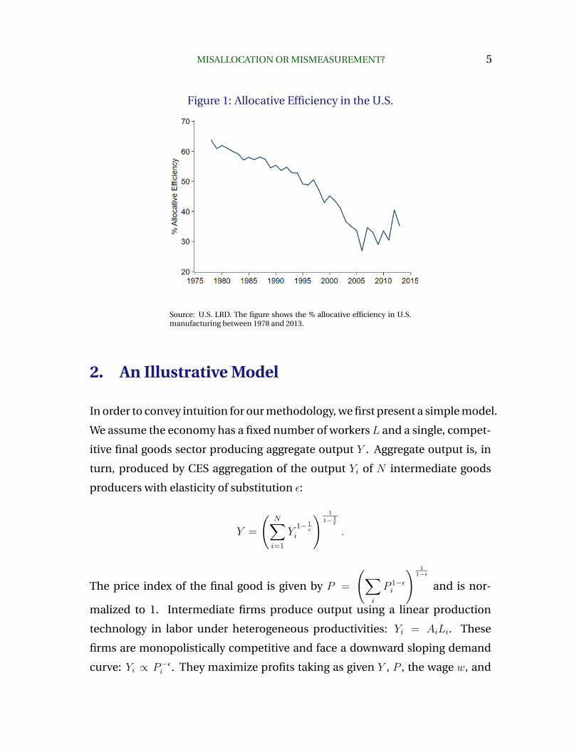
We first report estimates of allocative efficiency without correcting for mea-
surement error. The U.S. exhibits a severe decline, seemingly going from pro-
ducing 3/5 as much as it could by equalizing marginal products across plants to
producing only 1/3 as much as it could. Figure 1 displays this pattern. If true,
this plunge reduced the annual TFP growth rate by 1.7 percent per year over
1978–2013. By comparison, we estimate that Indian manufacturing operated at
about 1/2 efficiency, with a fair bit of volatility from year to year but no clear
trend despite major policy reforms. Thus by the end of the sample the U.S.
appears to have lower allocative efficiency than India.
Once we correct for measurement error, U.S. allocative efficiency is much
higher (above 2/3) with a modest downward trend and much less volatility.
Measurement error appears to be a growing problem in Census LRD plant data.
In the Indian ASI, correcting for measurement error has a less dramatic effect.
As a result, corrected allocative efficiency appears consistently higher in the
U.S., raising manufacturing productivity by 10 to 50 percent relative to that in
India (in all but one year).
The rest of the paper proceeds as follows. Section 2 presents a simple model
wherein both measurement error and distortions are fixed over time. Section 3
presents the full model, which allows both measurement error and distortions
to change over time. Section 4 describes the U.S. and Indian datasets, and raw
allocative efficiency patterns in the absence of our correction for measurement
error. Section 5 lays out our method for quantifying measurement error, and
applies it to the panel data on manufacturing plants in the U.S. and India. As
stated, these estimates impose the strong assumption that measurement error
and true productivity are uncorrelated. We also rely on local approximations,
so in Section 6 we examine how well our measure performs under alternative
assumptions on the properties of shocks to productivity, distortions, and mea-
surement error. Section 7 shows how correcting for measurement error affects
the picture of allocative efficiency in the U.S. and India.
MISALLOCATION OR MISMEASUREMENT? 5
Figure 1: Allocative Efficiency in the U.S.
Source: U.S. LRD. The figure shows the % allocative efficiency in U.S.manufacturing between 1978 and 2013.
2. An Illustrative Model
In order to convey intuition for our methodology, we first present a simple model.
We assume the economy has a fixed number of workers L and a single, compet-
itive final goods sector producing aggregate output Y . Aggregate output is, in
turn, produced by CES aggregation of the output Yi of N intermediate goods
producers with elasticity of substitution ε:
Y =
(N∑i=1
Y1− 1
εi
) 1
1− 1ε
.
The price index of the final good is given by P =
(∑i
P 1−εi
) 11−ε
and is nor-
malized to 1. Intermediate firms produce output using a linear production
technology in labor under heterogeneous productivities: Yi = AiLi. These
firms are monopolistically competitive and face a downward sloping demand
curve: Yi ∝ P−εi . They maximize profits taking as given Y , P , the wage w, and

6 BILS, KLENOW, AND RUANE
an idiosyncratic revenue distortion τi:
Πi =1
τiPiYi − wLi .
The researcher observes only measured revenue PiYi ≡ PiYi + gi and mea-
sured labor Li ≡ Li+fi. Given the assumed CES demand structure, firms charge
a common markup over their marginal cost (gross of the distortion):
Pi =
(ε
ε− 1
)×(τi ·
w
Ai
).
True revenue is therefore proportional to the product of true labor times and
the idiosyncratic distortion:
PiYi ∝ τi · Li . (1)
Thus variation across firms in true average revenue products(PiYiLi
)is solely
due to the distortion. Variation in measured average revenue products (TFPR),
however, reflects both the distortion and measurement errors:
TFPRi ≡PiYi
Li∝[τi ×
1 + gi/(PiYi)
1 + fi/Li
].
While our methodology will allow both the true distortions and measurement
errors to vary over time, to convey intuition we make the a number of simplify-
ing assumptions in this section:
1. The true distortions τi are fixed over time
2. The additive measurement error terms gi and fi are fixed over time
3. The idiosyncratic productivities Ait are time-varying
MISALLOCATION OR MISMEASUREMENT? 7
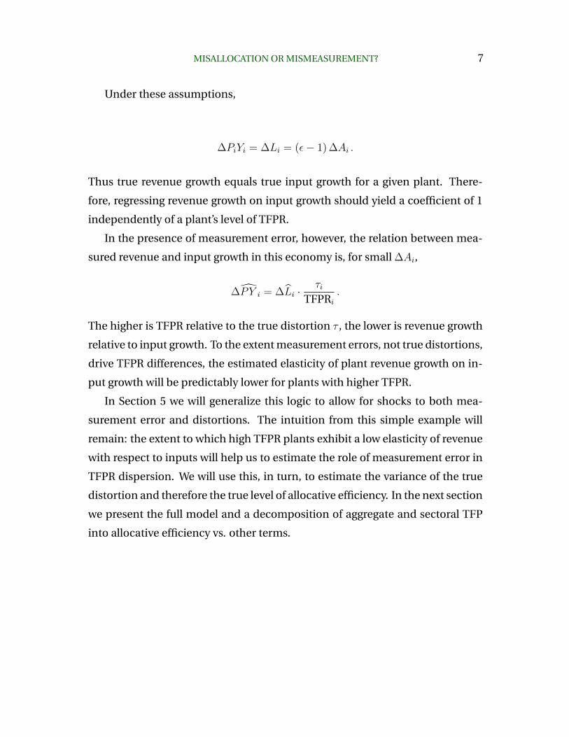
Under these assumptions,
∆PiYi = ∆Li = (ε− 1) ∆Ai .
Thus true revenue growth equals true input growth for a given plant. There-
fore, regressing revenue growth on input growth should yield a coefficient of 1
independently of a plant’s level of TFPR.
In the presence of measurement error, however, the relation between mea-
sured revenue and input growth in this economy is, for small ∆Ai,
∆P Y i = ∆Li ·τi
TFPRi
.
The higher is TFPR relative to the true distortion τ , the lower is revenue growth
relative to input growth. To the extent measurement errors, not true distortions,
drive TFPR differences, the estimated elasticity of plant revenue growth on in-
put growth will be predictably lower for plants with higher TFPR.
In Section 5 we will generalize this logic to allow for shocks to both mea-
surement error and distortions. The intuition from this simple example will
remain: the extent to which high TFPR plants exhibit a low elasticity of revenue
with respect to inputs will help us to estimate the role of measurement error in
TFPR dispersion. We will use this, in turn, to estimate the variance of the true
distortion and therefore the true level of allocative efficiency. In the next section
we present the full model and a decomposition of aggregate and sectoral TFP
into allocative efficiency vs. other terms.

8 BILS, KLENOW, AND RUANE
3. Model
3.1. Economic Environment
We consider an economy with S sectors, L workers and an exogenous capital
stock K. There are an exogenous number of firms Ns operating in each sector.
A representative firm produces a single final good Q in a perfectly competitive
final output market. This final good is produced using gross output Qst from
each sector s with a Cobb-Douglas production technology:
Q =S∏s=1
Qθss where
S∑s=1
θs = 1 .
We normalize P , the price of the final good, to 1. The final good can either be
consumed or used as an intermediate input:
Q = C +X .
All firms use the same intermediate input, with the amounts denotedXsi so that
X ≡S∑s=1
Xs =S∑s=1
Ns∑i=1
Xsi .
Sectoral output Qs is a CES aggregate of the outputs of the Ns sector-s firms:
Qs =
(Ns∑i=1
Q1− 1
εsi
) 1
1− 1ε
.
We denote by Ps the price index of output from sector s. Firms have idiosyn-
cratic productivity draws Asi, and produce output Qsi using a Cobb-Douglas
technology in capital, labor and intermediate inputs:
Qsi = Asi(Kαssi L
1−αssi )γsX1−γs
si where 0 < αs, γs < 1 .
The output elasticitiesαs and γs are sector-specific, but time-invariant and com-
mon across firms within a sector. Firms are monopolistically competitive and

MISALLOCATION OR MISMEASUREMENT? 9
face a downward sloping demand curve given by Qsi = Qs
(PsiPs
)−ε. Firms treat
Ps andQs as exogenous. Firms also face idiosyncratic labor distortions τLsi, capi-
tal distortions τKsi and intermediate input distortions τXsi . They maximize profits
Πsi taking input prices as given.
Πsi = Rsi − (1 + τLsi)wLsi − (1 + τKsi )rKsi − (1 + τXsi )PXsi ,
where Rsi ≡ PsiQsi is firm revenue.
3.2. Aggregate TFP
We define aggregate TFP as aggregate real consumption (or equivalently value-
added) divided by an appropriately weighted Cobb-Douglas bundle of aggre-
gate capital and labor:
TFP ≡ C
L1−αK αwhere α ≡
∑Ss=1 αsγsθs∑Ss=1 γsθs
.
We show in our Online Appendix that
TFP = T ×S∏s=1
TFP
θs∑Ss=1 γsθs
s .
T captures the effect of the sectoral distortions τLs , τKs and τXs , which are the
revenue-weighted harmonic means of the idiosyncratic firm-level distortions.3
Sectoral TFP is then:
TFPs ≡Qs
(Kαss L
1−αss )γsX1−γs
s
.
Within-sector misallocation lowers TFPs. The sectoral distortions will in-
3(1+ τLs ) ≡
[Ns∑i=1
RsiRs
1
1 + τLsi
]−1
and similarly for (1+ τKs ) and (1+ τXs ). The Online Appendix
expresses sectoral distortions as a function only of firm distortions and productivities.
10 BILS, KLENOW, AND RUANE
duce a cross-sector misallocation of resources, which will show up in T . While
cross-sector misallocation is of interest, it is not the focus of this paper. We
therefore leave it to future research to determine how important this could be
in determining cross-country aggregate TFP gaps.
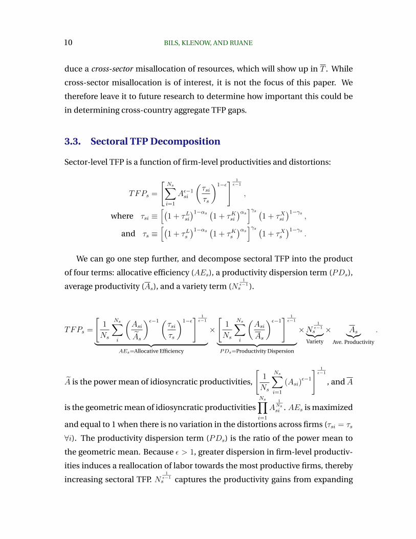
3.3. Sectoral TFP Decomposition
Sector-level TFP is a function of firm-level productivities and distortions:
TFPs =
[Ns∑i=1
Aε−1si
(τsiτs
)1−ε] 1ε−1
,
where τsi ≡[(
1 + τLsi)1−αs (
1 + τKsi)αs]γs (
1 + τXsi)1−γs
,
and τs ≡[(
1 + τLs)1−αs (
1 + τKs)αs]γs (
1 + τXs)1−γs
.
We can go one step further, and decompose sectoral TFP into the product
of four terms: allocative efficiency (AEs), a productivity dispersion term (PDs),
average productivity (As), and a variety term (N1ε−1s ).
TFPs =
[1
Ns
Ns∑i
(Asi
As
)ε−1(τsiτs
)1−ε] 1ε−1
︸ ︷︷ ︸AEs=Allocative Efficiency
×
[1
Ns
Ns∑i
(Asi
As
)ε−1] 1ε−1
︸ ︷︷ ︸PDs=Productivity Dispersion
×N1ε−1s︸ ︷︷ ︸
Variety
× As︸︷︷︸Ave. Productivity
.
A is the power mean of idiosyncratic productivities,
[1
Ns
Ns∑i=1
(Asi)ε−1
] 1ε−1
, and A
is the geometric mean of idiosyncratic productivitiesNs∏i=1
A1Nssi . AEs is maximized
and equal to 1 when there is no variation in the distortions across firms (τsi = τs
∀i). The productivity dispersion term (PDs) is the ratio of the power mean to
the geometric mean. Because ε > 1, greater dispersion in firm-level productiv-
ities induces a reallocation of labor towards the most productive firms, thereby
increasing sectoral TFP. N1ε−1s captures the productivity gains from expanding

MISALLOCATION OR MISMEASUREMENT? 11
the set of varieties available to sectoral goods producers. Finally, it is clear why
increases in average productivity (As) should increase sectoral TFP.
The goal of this paper is to present a methodology for inferring allocative
efficiency (AEs) from plant-level data while allowing for measurement error. In
the next section we briefly describe the U.S. and Indian datasets we use, present
the model-based approach to inferring allocative efficiency in the absence of
measurement error, and show raw allocative efficiency patterns in the data.
4. Inferring Allocative Efficiency
4.1. The Datasets
We use two datasets of manufacturing plants in this paper: the Indian Annual
Survey of Industries (ASI) from 1985 to 2013 and the U.S. Longitudinal Research
Database (LRD) from 1978 to 2013.
The ASI is a nationally representative survey of formal manufacturing plants
in India. The coverage includes plants with at least 10 workers using power,
and plants with at least 20 workers not using power. Plants fall into two cate-
gories: Census and Sample. Census plants are surveyed every year, and consist
of plants with at least 100 workers (the threshold increases to 200 workers in
some survey years) as well as all plants in 12 of the “industrially backwards”
states. Sample plants are randomly sampled each year within state × industry
cells. Official panel identifiers are available from 1998 on, and we use panel
identifiers from an old version of the publicly available ASI prior to 1998. We
construct an industry classification consisting of 50 manufacturing industries
which are consistently defined throughout our time period.4
The LRD is a database of U.S. manufacturing plants put together by the
U.S. Census Bureau. The coverage is all manufacturing plants with at least
one employee. The database includes information from the Annual Survey of
4The official sectoral classification (NIC) changed in 1987, 1998, 2004 and 2008. We useofficial NIC concordances to construct our harmonized classification.
12 BILS, KLENOW, AND RUANE
Manufactures (ASM) and the Census of Manufactures (CMF), augmented with
establishment identifiers from the Longitudinal Business Database (LBD). The
CMF is a census which is conducted in years ending in 2 or 7. The ASM is
a survey which is conducted in all other years. The ASM covers large plants
with certainty (typically plants with at least 100 workers, though the threshold
varies by survey year) and randomly samples smaller plants. The ASM sample
is redrawn in years ending in 4 and 9. In order to avoid any large changes in
sample size over time, we use only the ‘ASM’ sample plants in CMF years. From
here on, we refer to our U.S. dataset as the LRD. We use the harmonized sectoral
classification from Fort and Klimek (2016) at the NAICS 3-digit level (86 sectors).
The main variables we use are gross output, labor costs, capital, inventories,
and intermediate inputs. We construct gross output as the sum of shipments,
changes in finished and semi-finished good inventories, and other revenues.
We construct intermediate inputs as the sum of materials, fuels and other ex-
penditures. We include unpaid family workers in our measure of labor in India.
We construct labor costs as the sum of wages, salaries, bonuses and supplemen-
tal labor costs. We set the capital stock as the sum of fixed assets and the stock
of inventories.5 Official sampling weights are used in all of our calculations. We
discuss more details about variable construction in our Online Appendix.
We clean the ASI and LRD using the same approach. We drop plants with
missing or negative values for any of the variables described above. We then
trim the 1% tails of TFPR and TFPQ deviations from the industry average in each
year (TFPR and TFPQ are defined in the next section). We describe these steps
in more detail in our Online Appendix. Our final sample sizes are 1,806,000
plant-years for the U.S. and 943,186 plant-years for India.6
5Because of data availability, we use the nominal book value of fixed assets in India, and thereal market value of fixed assets in the U.S. Book value capital stocks are not reported everyyear in the U.S., unlike investment in fixed assets. Our real capital stock measure is constructedusing the perpetual inventory method. We do not deflate any nominal variables. Industry-leveldeflators would difference out because all of our analyses focus on within-industry differencesacross plants.
6We round U.S. observation counts in accordance with Census data disclosure rules.
MISALLOCATION OR MISMEASUREMENT? 13
4.2. Inferring Allocative Efficiency
Continuing to use ’s to denote measured values, TFPR and TFPQ are:
TFPRsi ≡Rsi
(KαssitL
1−αssi )γsX1−γs
si
,
(2)
TFPQsi ≡
(Rsit
) εε−1
(Kαssi L
1−αssi )γsX1−γs
si
.
In the absence of measurement error, TFPR would be proportional to the dis-
tortion and TFPQ would be proportional to productivity:
Rsi
(Kαssi L
1−αssi )γsX1−γs
si
∝ τsi and(Rsi)
εε−1
(Kαssi L
1−αssi )γsX1−γs
si
∝ Asi .
We infer sectoral allocative efficiency using the following expression:
AEs =
[Ns∑i=1
(TFPQsi
TFPQs
)ε−1(TFPRsi
TFPRs
)1−ε] 1ε−1
,
where TFPQs =
[Ns∑i=1
TFPQε−1si
] 1ε−1
,
and TFPRs =
(ε
ε− 1
)[MRPLs
(1− αs)γs
](1−αs)γs [MRPKs
αsγs
]αsγs [MRPXs1− γs
]1−γs.
MRPLs, MRPKs and MRPXs are the revenue-weighted harmonic mean values of
the marginal products of labor, capital and intermediates, respectively. E.g.,
MRPKs =
[∑i
Rsi
Rs
1
MRPKsi
]−1
,
MRPKsi =
(ε− 1
ε
)αsγs
Rst
Ksi
.
Aggregating across sectors we obtain inferred aggregate allocative efficiency,

14 BILS, KLENOW, AND RUANE
which is equal to true allocative efficiency when there is no measurement error:
AEt =S∏s=1
AE
θst∑Ss=1 γsθst
st .
In order to obtain estimates of allocative efficiency over time for the U.S.
and India we need to pin down a number of parameters in the model. Based on
evidence from Redding and Weinstein (2019), we pick a value of ε = 4 for the
elasticity of substitution across plants. Allocative inefficiencies are amplified
under higher values of this elasticity. We infer αs and γs based on country-
specific average sectoral cost shares.7 We allow the aggregate output shares θst
to vary across years, and base them on country-specific sectoral shares of man-
ufacturing output.8 We use labor costs as our measure of labor input because it
captures variation in human capital and hours worked across plants.
4.3. Time-Series Results
Figure 2 plots inferred allocative efficiency for India and the U.S. over their
respective samples. While allocative efficiency exhibits no clear trend in India,
there is a remarkable decrease in allocative efficiency in the U.S. from 1978
to 2006. As a result, over the entire sample allocative efficiency surprisingly
averages the same 48% for both India and the United States.9 Figure 3 plots
the ratio of U.S. to Indian allocative efficiency for their overlapping samples.
Allocative efficiency is lower in the U.S. than in India by around the year 2000
— substantially lower, as U.S. allocative efficiency averages only two-thirds of
Indian allocative efficiency from 2003 to 2013.
7We assume a rental rate for fixed assets of 20% and a rental rate of 10% for inventories.8Our results are not sensitive to the choice of constant or time-varying sectoral shares.9Average gains from full reallocation are 123% for the U.S. versus 111% for India. In contrast,
Hsieh and Klenow (2009) found 40-60% higher potential gains from reallocation in India thanin the United States. Our estimates diverge from Hsieh and Klenow’s for several reasons: Weuse gross output while they use value added; we have a 1978–2013 LRD sample while they have1987, 1992, and 1997 Census plants; we trim 1% tails in the U.S., while they trim 2%. (Theyinconsistently trimmed 2% for the U.S. and only 1% for India.)

MISALLOCATION OR MISMEASUREMENT? 15
Figure 2: Allocative Efficiency in India and the U.S.
India U.S.
Source: Indian ASI and U.S. LRD. The figure shows the % allocative efficiency for both countries. Averageallocative efficiency is 49% in India and 54% in the U.S. over the respective sample periods.
Figure 3: Allocative Efficiency, U.S. Relative to India
Source: Indian ASI and U.S. LRD. The figure plots the ratio of U.S. allocative efficiency toIndian allocative efficiency for the years 1985 to 2007 (years in which the datasets overlap).
16 BILS, KLENOW, AND RUANE
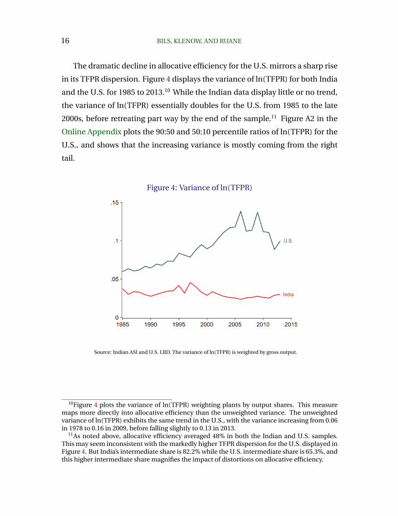
The dramatic decline in allocative efficiency for the U.S. mirrors a sharp rise
in its TFPR dispersion. Figure 4 displays the variance of ln(TFPR) for both India
and the U.S. for 1985 to 2013.10 While the Indian data display little or no trend,
the variance of ln(TFPR) essentially doubles for the U.S. from 1985 to the late
2000s, before retreating part way by the end of the sample.11 Figure A2 in the
Online Appendix plots the 90:50 and 50:10 percentile ratios of ln(TFPR) for the
U.S., and shows that the increasing variance is mostly coming from the right
tail.
Figure 4: Variance of ln(TFPR)
Source: Indian ASI and U.S. LRD. The variance of ln(TFPR) is weighted by gross output.
10Figure 4 plots the variance of ln(TFPR) weighting plants by output shares. This measuremaps more directly into allocative efficiency than the unweighted variance. The unweightedvariance of ln(TFPR) exhibits the same trend in the U.S., with the variance increasing from 0.06in 1978 to 0.16 in 2009, before falling slightly to 0.13 in 2013.
11As noted above, allocative efficiency averaged 48% in both the Indian and U.S. samples.This may seem inconsistent with the markedly higher TFPR dispersion for the U.S. displayed inFigure 4. But India’s intermediate share is 82.2% while the U.S. intermediate share is 65.3%, andthis higher intermediate share magnifies the impact of distortions on allocative efficiency.

MISALLOCATION OR MISMEASUREMENT? 17
Figure A3 in the Online Appendix shows that TFPQ dispersion rose in both
the U.S. and India from 1985–2013. The variance in logs rose from about 0.35
to 0.45 or more in both countries. At the same time, the elasticity of TFPR
with respect to TFPQ rose in the U.S. while falling in India — see Figure A4 in
the Online Appendix. The elasticity rose from around 0.27 to 0.37 in the U.S.
from 1985 to 2013. Gouin-Bonenfant (2019) formulates a theory in which ris-
ing TFPQ dispersion is responsible for both rising TFPR dispersion (and falling
labor share of income) in the U.S. in recent decades. In Section 7 we examine
how correcting for measurement error alters these patterns, in addition to its
impact on trends in allocative efficiency.
In the next section we present out methodology to correct TFPR for mea-
surement errors with the goal of obtaining measures of allocative efficiency that
are more robust to such errors.
5. Measurement Error
Calculations of misallocation, including those just presented, interpret plant
differences in measured average revenue products (TFPR) as differences in true
marginal products. In many of these studies the underlying plant data are lon-
gitudinal. We will show that, using such data, one can project the elasticity of
revenue with respect to inputs on TFPR to answer the question: to what extent
do plants with higher measured average products have higher true marginal
products? The logic is similar to using the covariance of two noisy measures of
a variable, here noisy measures of a plant’s marginal revenue product, to recover
a truer measure of the variable.
18 BILS, KLENOW, AND RUANE
5.1. Measurement Error and TFPR
Consider the following description of measured inputs I and measured revenue
R for plant i (year subscripts implicit):
Ii ≡ φi · Ii + fi ,
Ri ≡ χi ·Ri + gi ,
where I and R denote true inputs and revenues, f and g reflect additive mea-
surement errors, and φ and χ are multiplicative errors.12 For simplicity, we treat
the impact of measurement error in inputs as common across different inputs
(capital, labor, intermediates).
In the setting of Section 2, profit maximization by each plant implies
TFPRi ≡Ri
Ii∝ τi
(Ri
Ri
Ii
Ii
).
Absent measurement error, a plant’s TFPR provides a measure of its distortion
τ . But, to the extent revenue is overstated or inputs are understated, TFPR will
overstate τ . In that circumstance, the plant’s marginal revenue product is less
than implied by its TFPR.
The growth rate of a plant’s TFPR will reflect the growth rate of its measure-
ment error as well as the growth rate of its τ :
∆TFPRi = ∆τi + ∆
(Ri
Ri
)− ∆
(IiIi
).
∆ denotes the growth rate of a plant variable relative to the mean in its sector.
If there are only additive measurement errors, then TFPR growth is
∆TFPRi ≈∆τi
Ri/Ri
−
(Ri −Ri
Ri
− Ii − IiIi
)∆Ii +
dgi
Ri
− dfi
Ii,
12Note that the additive terms f and g could alternatively reflect deviations from Cobb-Douglas production. For instance, positive values for f (such as overhead inputs), or negativefor g, would imply marginal revenue exceeds average revenue per input.
MISALLOCATION OR MISMEASUREMENT? 19
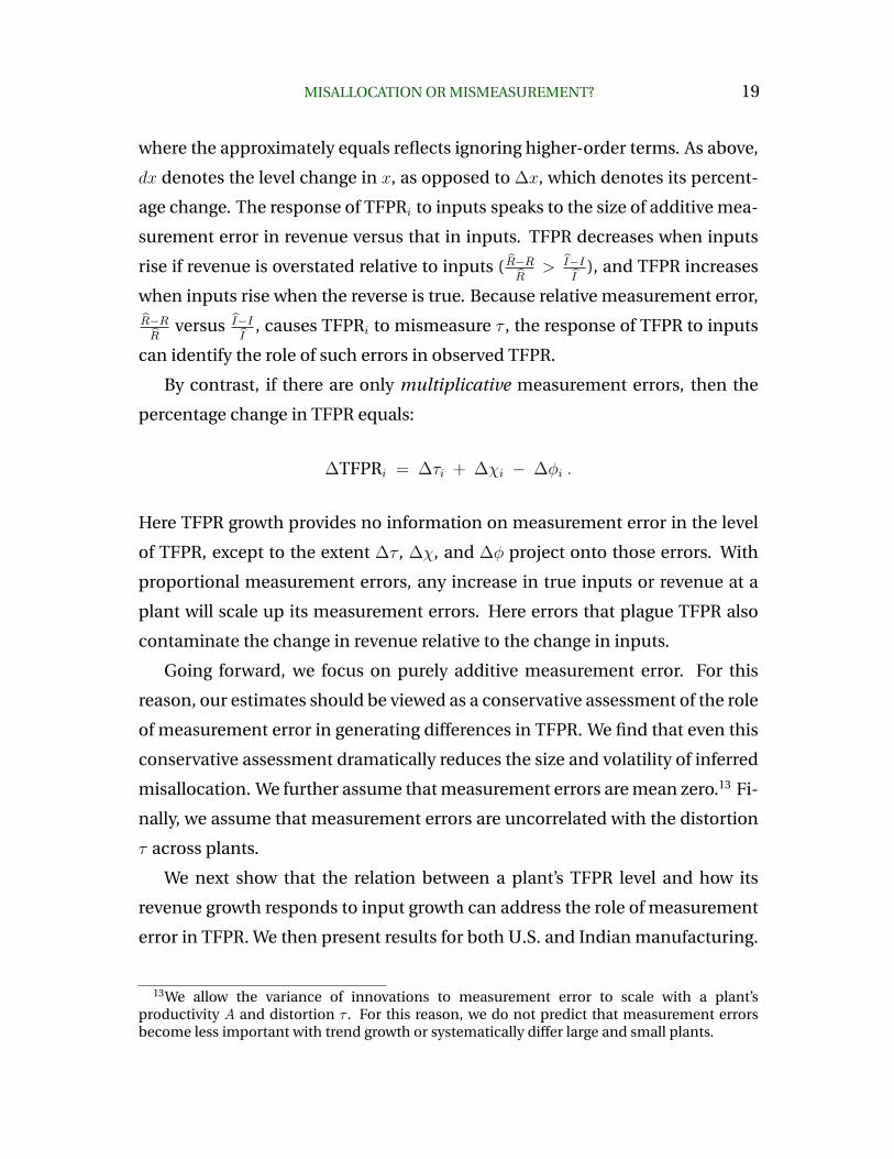
where the approximately equals reflects ignoring higher-order terms. As above,
dx denotes the level change in x, as opposed to ∆x, which denotes its percent-
age change. The response of TFPRi to inputs speaks to the size of additive mea-
surement error in revenue versus that in inputs. TFPR decreases when inputs
rise if revenue is overstated relative to inputs ( R−RR
> I−II
), and TFPR increases
when inputs rise when the reverse is true. Because relative measurement error,R−RR
versus I−II
, causes TFPRi to mismeasure τ , the response of TFPR to inputs
can identify the role of such errors in observed TFPR.
By contrast, if there are only multiplicative measurement errors, then the
percentage change in TFPR equals:
∆TFPRi = ∆τi + ∆χi − ∆φi .
Here TFPR growth provides no information on measurement error in the level
of TFPR, except to the extent ∆τ , ∆χ, and ∆φ project onto those errors. With
proportional measurement errors, any increase in true inputs or revenue at a
plant will scale up its measurement errors. Here errors that plague TFPR also
contaminate the change in revenue relative to the change in inputs.
Going forward, we focus on purely additive measurement error. For this
reason, our estimates should be viewed as a conservative assessment of the role
of measurement error in generating differences in TFPR. We find that even this
conservative assessment dramatically reduces the size and volatility of inferred
misallocation. We further assume that measurement errors are mean zero.13 Fi-
nally, we assume that measurement errors are uncorrelated with the distortion
τ across plants.
We next show that the relation between a plant’s TFPR level and how its
revenue growth responds to input growth can address the role of measurement
error in TFPR. We then present results for both U.S. and Indian manufacturing.
13We allow the variance of innovations to measurement error to scale with a plant’sproductivity A and distortion τ . For this reason, we do not predict that measurement errorsbecome less important with trend growth or systematically differ large and small plants.

20 BILS, KLENOW, AND RUANE
5.2. Identifying Measurement Error
Our focal point is the elasticity of measured revenue with respect to measured
inputs, conditional on plant TFPR taking a particular value–call it TFPRk:
βk ≡Covk(∆Ri,∆Ii)
Vark(∆Ii).
For exposition we first assume no measurement error, then allow for errors
in both revenue and inputs. Absent measurement error, changes in revenue
and inputs simply reflect changes in the plant’s productivity and distortion:
∆Ii = ∆Ii = (ε− 1) ∆Ai − ε∆τi ,
(3)
∆Ri = ∆Ri = (ε− 1)(∆Ai −∆τi) .
So βk is given by:
βk = 1 + φk , (4)
where φk ≡Covk(∆τi,∆Ii)
Vark(∆Ii)=−ε · Vark(∆τi) + (ε− 1) · Covk(∆τi,∆Ai)
Vark(∆Ii).
φk is the elasticity of ∆τ with respect to ∆I.
βk reflects a standard inference problem: a given increase in inputs creates
a larger response in revenue if it is driven by A than if it is driven by a decline in
τ . If Vark (∆τ) = 0 then βk = 1, whereas if Vark (∆A) = 0 then βk = ε−1ε< 1. If τ
follows a random walk so that ∆τ is i.i.d., then βk reduces to 1 + φ regardless of
TFPR. For stationary τ , its conditional volatility is greater at extreme τ ’s, reflect-
ing τ ’s regression back to its mean. Thus the Vark(∆τ) is greater at extremes for
TFPR, implying smaller values for βk.
MISALLOCATION OR MISMEASUREMENT? 21
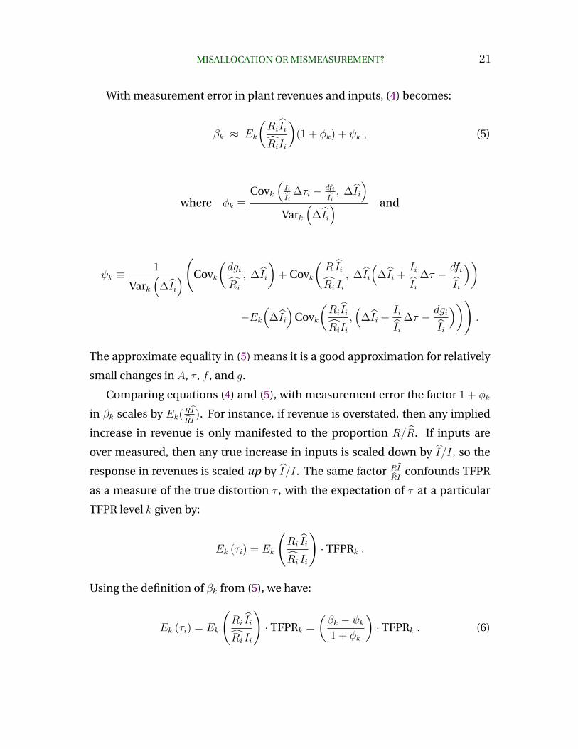
With measurement error in plant revenues and inputs, (4) becomes:
βk ≈ Ek
(RiIi
RiIi
)(1 + φk) + ψk , (5)
where φk ≡Covk
(IiIi
∆τi − dfiIi, ∆Ii
)Vark
(∆Ii
) and
ψk ≡1
Vark(
∆Ii
)(Covk
(dgi
Ri
, ∆Ii
)+ Covk
(RIi
Ri Ii, ∆Ii
(∆Ii +
Ii
Ii∆τ − dfi
Ii
))
−Ek(
∆Ii
)Covk
(RiIi
RiIi,(
∆Ii +Ii
Ii∆τ − dgi
Ii
))).
The approximate equality in (5) means it is a good approximation for relatively
small changes in A, τ , f , and g.
Comparing equations (4) and (5), with measurement error the factor 1 + φk
in βk scales by Ek(RIRI ). For instance, if revenue is overstated, then any implied
increase in revenue is only manifested to the proportion R/R. If inputs are
over measured, then any true increase in inputs is scaled down by I/I, so the
response in revenues is scaled up by I/I. The same factor RI
RIconfounds TFPR
as a measure of the true distortion τ , with the expectation of τ at a particular
TFPR level k given by:
Ek (τi) = Ek
(Ri Ii
Ri Ii
)· TFPRk .
Using the definition of βk from (5), we have:
Ek (τi) = Ek
(Ri Ii
Ri Ii
)· TFPRk =
(βk − ψk1 + φk
)· TFPRk . (6)
22 BILS, KLENOW, AND RUANE
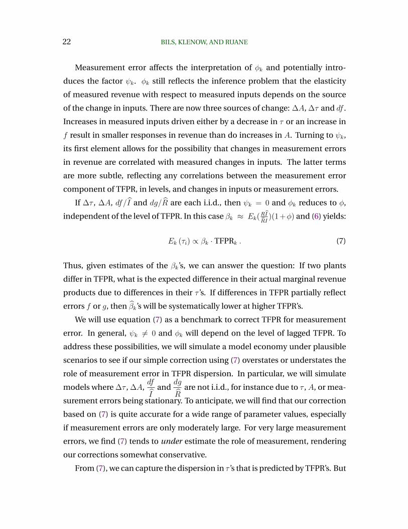
Measurement error affects the interpretation of φk and potentially intro-
duces the factor ψk. φk still reflects the inference problem that the elasticity
of measured revenue with respect to measured inputs depends on the source
of the change in inputs. There are now three sources of change: ∆A, ∆τ and df .
Increases in measured inputs driven either by a decrease in τ or an increase in
f result in smaller responses in revenue than do increases in A. Turning to ψk,
its first element allows for the possibility that changes in measurement errors
in revenue are correlated with measured changes in inputs. The latter terms
are more subtle, reflecting any correlations between the measurement error
component of TFPR, in levels, and changes in inputs or measurement errors.
If ∆τ , ∆A, df/I and dg/R are each i.i.d., then ψk = 0 and φk reduces to φ,
independent of the level of TFPR. In this case βk ≈ Ek(RI
RI)(1+φ) and (6) yields:
Ek (τi) ∝ βk · TFPRk . (7)
Thus, given estimates of the βk’s, we can answer the question: If two plants
differ in TFPR, what is the expected difference in their actual marginal revenue
products due to differences in their τ ’s. If differences in TFPR partially reflect
errors f or g, then βk’s will be systematically lower at higher TFPR’s.
We will use equation (7) as a benchmark to correct TFPR for measurement
error. In general, ψk 6= 0 and φk will depend on the level of lagged TFPR. To
address these possibilities, we will simulate a model economy under plausible
scenarios to see if our simple correction using (7) overstates or understates the
role of measurement error in TFPR dispersion. In particular, we will simulate
models where ∆τ , ∆A,df
Iand
dg
Rare not i.i.d., for instance due to τ , A, or mea-
surement errors being stationary. To anticipate, we will find that our correction
based on (7) is quite accurate for a wide range of parameter values, especially
if measurement errors are only moderately large. For very large measurement
errors, we find (7) tends to under estimate the role of measurement, rendering
our corrections somewhat conservative.
From (7), we can capture the dispersion in τ ’s that is predicted by TFPR’s. But

MISALLOCATION OR MISMEASUREMENT? 23
in the presence of measurement error there will also be differences in τ ’s that are
orthogonal to TFPR. For instance, a plant with a high value for τ but understated
revenue might display purely average TFPR. To capture this component, we
“add back” variation in τ ’s that is orthogonal to TFPR, under an assumption
that true τ is orthogonal to the measurement error component of TFPR.
From the relation between TFPR, τ , and measurement error, we have:
Var(
ln τi
)= Var
(ln TFPRi
)− Var
(ln
(Ri Ii
Ri Ii
))+ 2Cov
(ln τi, ln
(Ri Ii
Ri Ii
)).
(8)
We assume that the two components of TFPR, namely the true distortion τ and
the measurement error component R I
R I, are orthogonal to each other in their
natural logs. This eliminates the last term in equation (8). Furthermore, the
middle term can be written as the two terms:14
−Var
(ln
(Ri Ii
Ri Ii
))= Cov
(ln TFPRk, Ek
(ln
(Ri Ii
Ri Ii
)))− Cov
(ln τi, ln
(Ri Ii
Ri Ii
)),
which reduces to its first term, given the assumption τ and R
R Iare orthogonal.
Thus equation (8) can be reduced to:
Var(
ln τi
)= Var
(ln TFPRi
)+ Cov
(ln TFPRk, Ek
(ln
(Ri Ii
Ri Ii
))). (9)
The first term is data. The second is provided by how the estimates of βk, dis-
cussed earlier in this subsection, covary with TFPR. We add back dispersion in τ
that is mean zero and orthogonal TFPR, with variance dictated by equation (9).
14This step uses that ln(R I
R I
)equals (− ln TFPR + ln τ) and that it can also be broken into
Ek
(ln
(R I
R I
))and
(ln(R I
R I
)− Ek
(ln
(R I
R I
))).
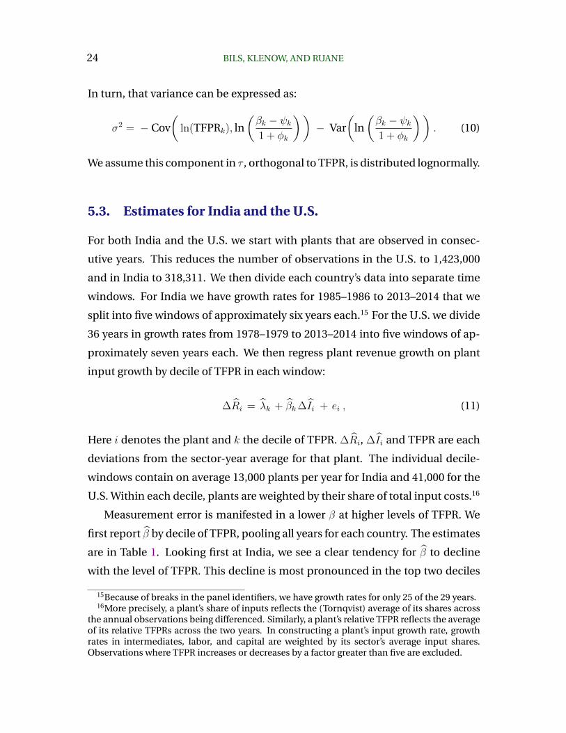
24 BILS, KLENOW, AND RUANE
In turn, that variance can be expressed as:
σ2 = − Cov(
ln(TFPRk), ln(βk − ψk1 + φk
))− Var
(ln(βk − ψk1 + φk
)). (10)
We assume this component in τ , orthogonal to TFPR, is distributed lognormally.
5.3. Estimates for India and the U.S.
For both India and the U.S. we start with plants that are observed in consec-
utive years. This reduces the number of observations in the U.S. to 1,423,000
and in India to 318,311. We then divide each country’s data into separate time
windows. For India we have growth rates for 1985–1986 to 2013–2014 that we
split into five windows of approximately six years each.15 For the U.S. we divide
36 years in growth rates from 1978–1979 to 2013–2014 into five windows of ap-
proximately seven years each. We then regress plant revenue growth on plant
input growth by decile of TFPR in each window:
∆Ri = λk + βk∆Ii + ei , (11)
Here i denotes the plant and k the decile of TFPR. ∆Ri, ∆Ii and TFPR are each
deviations from the sector-year average for that plant. The individual decile-
windows contain on average 13,000 plants per year for India and 41,000 for the
U.S. Within each decile, plants are weighted by their share of total input costs.16
Measurement error is manifested in a lower β at higher levels of TFPR. We
first report β by decile of TFPR, pooling all years for each country. The estimates
are in Table 1. Looking first at India, we see a clear tendency for β to decline
with the level of TFPR. This decline is most pronounced in the top two deciles
15Because of breaks in the panel identifiers, we have growth rates for only 25 of the 29 years.16More precisely, a plant’s share of inputs reflects the (Tornqvist) average of its shares across
the annual observations being differenced. Similarly, a plant’s relative TFPR reflects the averageof its relative TFPRs across the two years. In constructing a plant’s input growth rate, growthrates in intermediates, labor, and capital are weighted by its sector’s average input shares.Observations where TFPR increases or decreases by a factor greater than five are excluded.
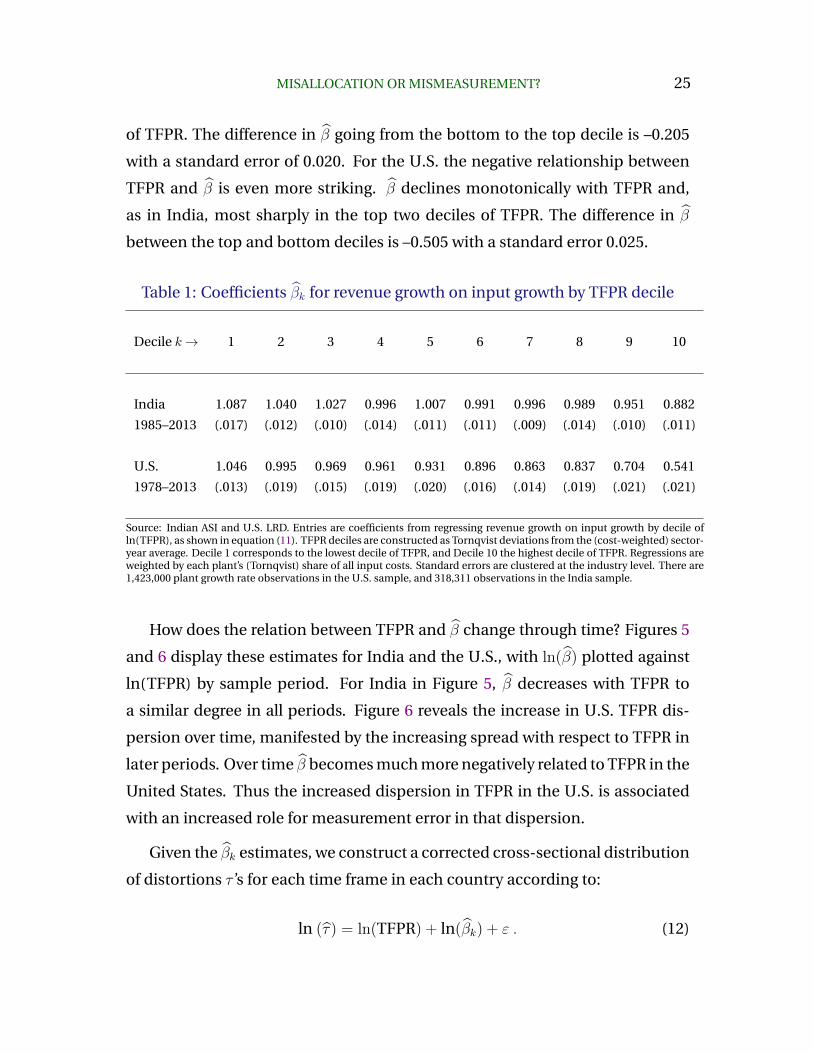
MISALLOCATION OR MISMEASUREMENT? 25
of TFPR. The difference in β going from the bottom to the top decile is –0.205
with a standard error of 0.020. For the U.S. the negative relationship between
TFPR and β is even more striking. β declines monotonically with TFPR and,
as in India, most sharply in the top two deciles of TFPR. The difference in β
between the top and bottom deciles is –0.505 with a standard error 0.025.
Table 1: Coefficients βk for revenue growth on input growth by TFPR decile
Decile k→ 1 2 3 4 5 6 7 8 9 10
India 1.087 1.040 1.027 0.996 1.007 0.991 0.996 0.989 0.951 0.882
1985–2013 (.017) (.012) (.010) (.014) (.011) (.011) (.009) (.014) (.010) (.011)
U.S. 1.046 0.995 0.969 0.961 0.931 0.896 0.863 0.837 0.704 0.541
1978–2013 (.013) (.019) (.015) (.019) (.020) (.016) (.014) (.019) (.021) (.021)
Source: Indian ASI and U.S. LRD. Entries are coefficients from regressing revenue growth on input growth by decile ofln(TFPR), as shown in equation (11). TFPR deciles are constructed as Tornqvist deviations from the (cost-weighted) sector-year average. Decile 1 corresponds to the lowest decile of TFPR, and Decile 10 the highest decile of TFPR. Regressions areweighted by each plant’s (Tornqvist) share of all input costs. Standard errors are clustered at the industry level. There are1,423,000 plant growth rate observations in the U.S. sample, and 318,311 observations in the India sample.
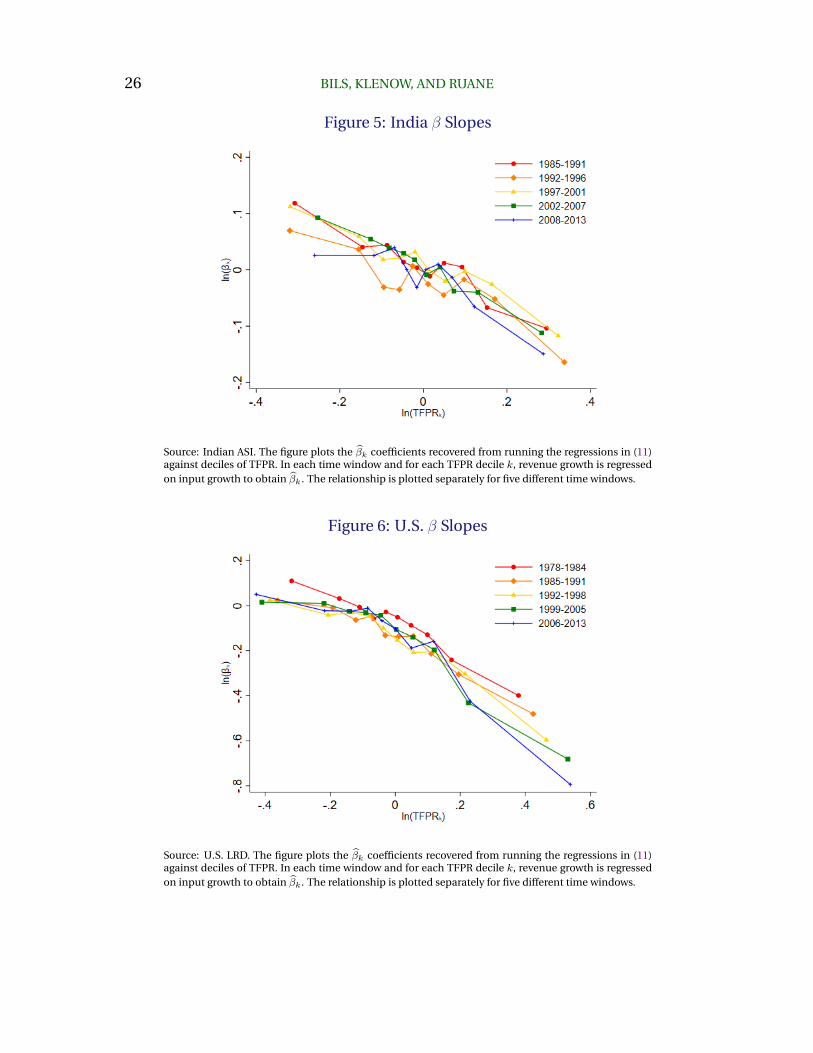
How does the relation between TFPR and β change through time? Figures 5
and 6 display these estimates for India and the U.S., with ln(β) plotted against
ln(TFPR) by sample period. For India in Figure 5, β decreases with TFPR to
a similar degree in all periods. Figure 6 reveals the increase in U.S. TFPR dis-
persion over time, manifested by the increasing spread with respect to TFPR in
later periods. Over time β becomes much more negatively related to TFPR in the
United States. Thus the increased dispersion in TFPR in the U.S. is associated
with an increased role for measurement error in that dispersion.
Given the βk estimates, we construct a corrected cross-sectional distribution
of distortions τ ’s for each time frame in each country according to:
ln (τ) = ln(TFPR) + ln(βk) + ε . (12)
26 BILS, KLENOW, AND RUANE
Figure 5: India β Slopes
Source: Indian ASI. The figure plots the βk coefficients recovered from running the regressions in (11)against deciles of TFPR. In each time window and for each TFPR decile k, revenue growth is regressedon input growth to obtain βk. The relationship is plotted separately for five different time windows.
Figure 6: U.S. β Slopes
Source: U.S. LRD. The figure plots the βk coefficients recovered from running the regressions in (11)against deciles of TFPR. In each time window and for each TFPR decile k, revenue growth is regressedon input growth to obtain βk. The relationship is plotted separately for five different time windows.
MISALLOCATION OR MISMEASUREMENT? 27
More exactly, each plant in a cross-sectional sample is assigned the βk estimated
for the TFPR decile corresponding to its TFPR.17 ε is drawn from a log normal
distribution, conditional on TFPR, with variance as dictated by equation (10).18
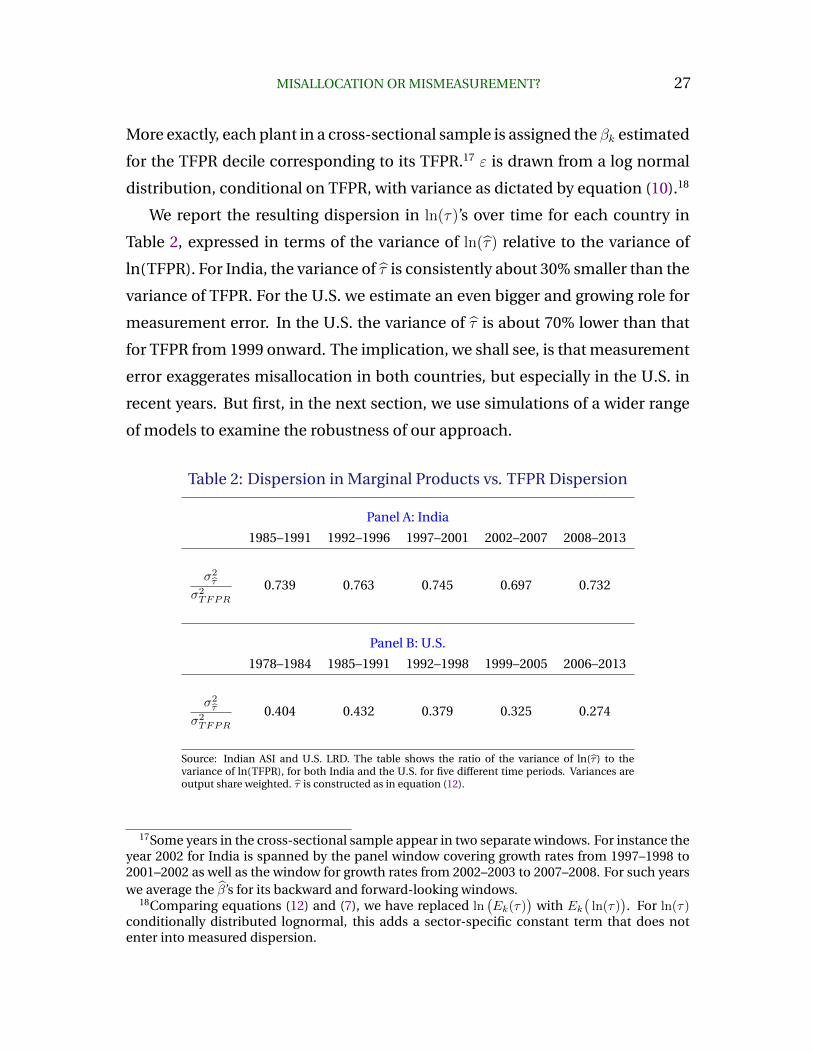
We report the resulting dispersion in ln(τ)’s over time for each country in
Table 2, expressed in terms of the variance of ln(τ) relative to the variance of
ln(TFPR). For India, the variance of τ is consistently about 30% smaller than the
variance of TFPR. For the U.S. we estimate an even bigger and growing role for
measurement error. In the U.S. the variance of τ is about 70% lower than that
for TFPR from 1999 onward. The implication, we shall see, is that measurement
error exaggerates misallocation in both countries, but especially in the U.S. in
recent years. But first, in the next section, we use simulations of a wider range
of models to examine the robustness of our approach.
Table 2: Dispersion in Marginal Products vs. TFPR Dispersion
Panel A: India
1985–1991 1992–1996 1997–2001 2002–2007 2008–2013
σ2τ
σ2TFPR
0.739 0.763 0.745 0.697 0.732
Panel B: U.S.
1978–1984 1985–1991 1992–1998 1999–2005 2006–2013
σ2τ
σ2TFPR
0.404 0.432 0.379 0.325 0.274
Source: Indian ASI and U.S. LRD. The table shows the ratio of the variance of ln(τ ) to thevariance of ln(TFPR), for both India and the U.S. for five different time periods. Variances areoutput share weighted. τ is constructed as in equation (12).
17Some years in the cross-sectional sample appear in two separate windows. For instance theyear 2002 for India is spanned by the panel window covering growth rates from 1997–1998 to2001–2002 as well as the window for growth rates from 2002–2003 to 2007–2008. For such yearswe average the β’s for its backward and forward-looking windows.
18Comparing equations (12) and (7), we have replaced ln(Ek(τ)
)with Ek
(ln(τ)
). For ln(τ)
conditionally distributed lognormal, this adds a sector-specific constant term that does notenter into measured dispersion.
28 BILS, KLENOW, AND RUANE
6. Robustness in Simulations
Our approach to estimating the share of true τ dispersion in TFPR dispersion
rests on a set of assumptions, most notably that measurement errors are addi-
tive and that their role in a plant’s TFPR is orthogonal to its true τ distortion.19
Furthermore, if innovations to A, τ , or measurement errors are not i.i.d., then
our corrections based on equation (6) are potentially clouded as terms φk and
ψk may influence the projection of βk on TFPR. Finally, our derivations rely
on first-order approximations which may not perform well for large shocks to
productivity, distortions or measurement errors.
For these reasons, we explore the performance of our estimator in simula-
tions. We match simulated moments to data moments for India and the United
State. We find that our estimator performs well even if measurement error is
sizable, such as we estimate for India. If measurement error is enormously
important, as we find for the U.S., then our approach is conservative, as it tends
to understate the role of measurement error in TFPR dispersion.
We assume that plant i’s idiosyncratic productivity in period t is given by:
Ait = Ai · ait .
Ai is the permanent component of a plant’s productivity, which we assume is
lognormally distributed: ln(Ai) ∼ N(0, σ2A). ait is the transitory component of
plant productivity. Plants also face an idiosyncratic, time-varying distortion τit.
ait and τit follow:
ln(ait) = ρa · ln(ait−1) + ηait where ηait ∼ N(0, σ2a) ,
(13)
ln(τit) = ρτ · ln(τit−1) + ητit where ητit ∼ N(0, σ2τ ) .
19Assuming that a firm’s τ is orthogonal to the size of its measurement errors f and g does nottranslate directly to orthogonality of τ and the measurement error component of TFPR, becausea plant’s τ affects its scale and thereby the relative importance of its measurement errors.
MISALLOCATION OR MISMEASUREMENT? 29
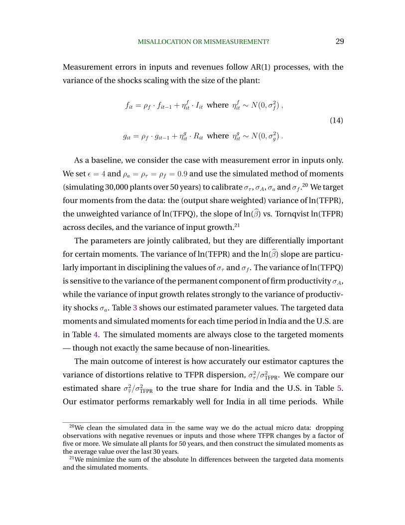
Measurement errors in inputs and revenues follow AR(1) processes, with the
variance of the shocks scaling with the size of the plant:
fit = ρf · fit−1 + ηfit · Iit where ηfit ∼ N(0, σ2f ) ,
(14)
git = ρf · git−1 + ηgit ·Rit where ηgit ∼ N(0, σ2g) .
As a baseline, we consider the case with measurement error in inputs only.
We set ε = 4 and ρa = ρτ = ρf = 0.9 and use the simulated method of moments
(simulating 30,000 plants over 50 years) to calibrate στ , σA, σa and σf .20 We target
four moments from the data: the (output share weighted) variance of ln(TFPR),
the unweighted variance of ln(TFPQ), the slope of ln(β) vs. Tornqvist ln(TFPR)
across deciles, and the variance of input growth.21
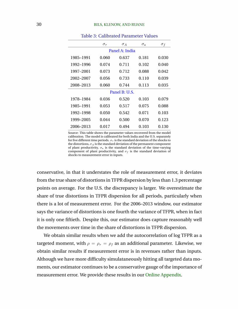
The parameters are jointly calibrated, but they are differentially important
for certain moments. The variance of ln(TFPR) and the ln(β) slope are particu-
larly important in disciplining the values of στ and σf . The variance of ln(TFPQ)
is sensitive to the variance of the permanent component of firm productivity σA,
while the variance of input growth relates strongly to the variance of productiv-
ity shocks σa. Table 3 shows our estimated parameter values. The targeted data
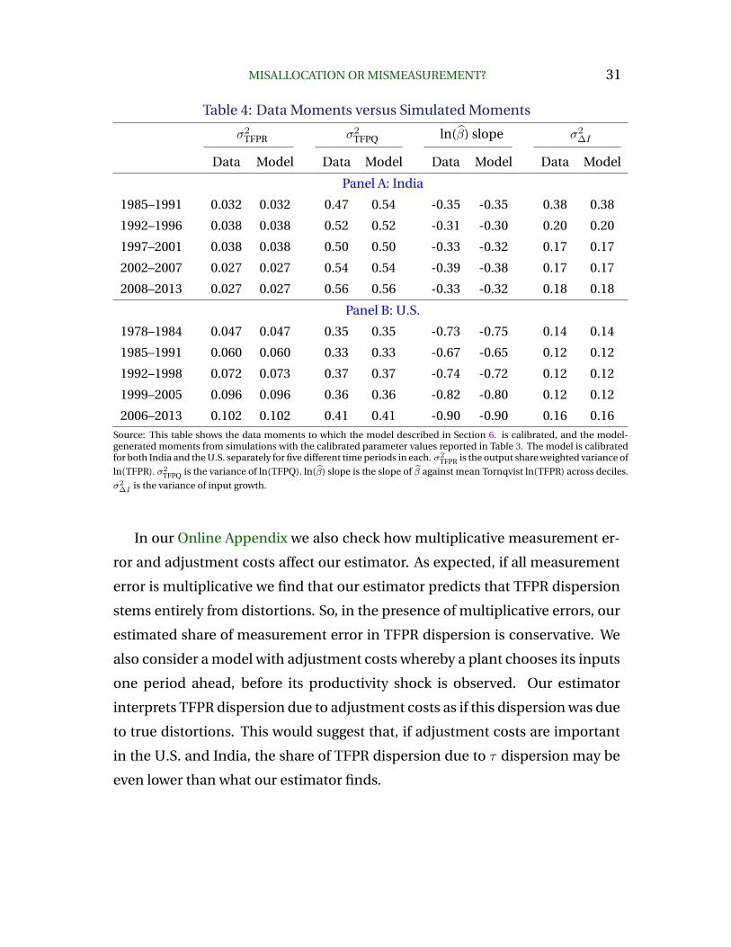
moments and simulated moments for each time period in India and the U.S. are
in Table 4. The simulated moments are always close to the targeted moments
— though not exactly the same because of non-linearities.
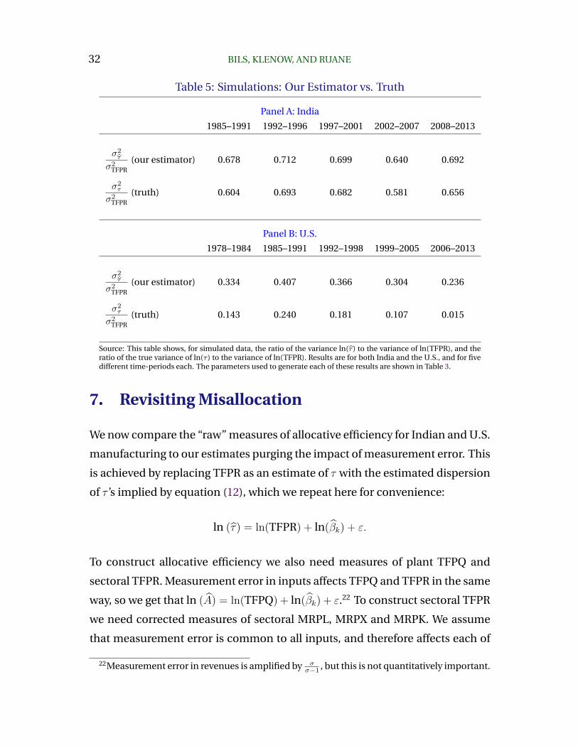
The main outcome of interest is how accurately our estimator captures the
variance of distortions relative to TFPR dispersion, σ2τ/σ
2TFPR. We compare our
estimated share σ2τ/σ
2TFPR to the true share for India and the U.S. in Table 5.
Our estimator performs remarkably well for India in all time periods. While
20We clean the simulated data in the same way we do the actual micro data: droppingobservations with negative revenues or inputs and those where TFPR changes by a factor offive or more. We simulate all plants for 50 years, and then construct the simulated moments asthe average value over the last 30 years.
21We minimize the sum of the absolute ln differences between the targeted data momentsand the simulated moments.
30 BILS, KLENOW, AND RUANE
Table 3: Calibrated Parameter Values
στ σA σa σf
Panel A: India
1985–1991 0.060 0.637 0.181 0.030
1992–1996 0.074 0.711 0.102 0.040
1997–2001 0.073 0.712 0.088 0.042
2002–2007 0.056 0.733 0.110 0.039
2008–2013 0.060 0.744 0.113 0.035
Panel B: U.S.
1978–1984 0.036 0.520 0.103 0.079
1985–1991 0.053 0.517 0.075 0.088
1992–1998 0.050 0.542 0.071 0.103
1999–2005 0.044 0.500 0.070 0.123
2006–2013 0.017 0.494 0.103 0.130Source: This table shows the parameter values recovered from the modelcalibration. The model is calibrated for both India and the U.S. separatelyfor five different time periods. στ is the standard deviation of the shocks tothe distortions, σA is the standard deviation of the permanent componentof plant productivity, σa is the standard deviation of the time-varyingcomponent of plant productivity, and σf is the standard deviation ofshocks to measurement error in inputs.
conservative, in that it understates the role of measurement error, it deviates
from the true share of distortions in TFPR dispersion by less than 1.3 percentage
points on average. For the U.S. the discrepancy is larger. We overestimate the
share of true distortions in TFPR dispersion for all periods, particularly when
there is a lot of measurement error. For the 2006–2013 window, our estimator
says the variance of distortions is one fourth the variance of TFPR, when in fact
it is only one fiftieth. Despite this, our estimator does capture reasonably well
the movements over time in the share of distortions in TFPR dispersion.
We obtain similar results when we add the autocorrelation of log TFPR as a
targeted moment, with ρ = ρτ = ρf as an additional parameter. Likewise, we
obtain similar results if measurement error is in revenues rather than inputs.
Although we have more difficulty simulataneously hitting all targeted data mo-
ments, our estimator continues to be a conservative gauge of the importance of
measurement error. We provide these results in our Online Appendix.
MISALLOCATION OR MISMEASUREMENT? 31
Table 4: Data Moments versus Simulated Moments
σ2TFPR σ2
TFPQ ln(β) slope σ2∆I
Data Model Data Model Data Model Data Model
Panel A: India
1985–1991 0.032 0.032 0.47 0.54 -0.35 -0.35 0.38 0.38
1992–1996 0.038 0.038 0.52 0.52 -0.31 -0.30 0.20 0.20
1997–2001 0.038 0.038 0.50 0.50 -0.33 -0.32 0.17 0.17
2002–2007 0.027 0.027 0.54 0.54 -0.39 -0.38 0.17 0.17
2008–2013 0.027 0.027 0.56 0.56 -0.33 -0.32 0.18 0.18
Panel B: U.S.
1978–1984 0.047 0.047 0.35 0.35 -0.73 -0.75 0.14 0.14
1985–1991 0.060 0.060 0.33 0.33 -0.67 -0.65 0.12 0.12
1992–1998 0.072 0.073 0.37 0.37 -0.74 -0.72 0.12 0.12
1999–2005 0.096 0.096 0.36 0.36 -0.82 -0.80 0.12 0.12
2006–2013 0.102 0.102 0.41 0.41 -0.90 -0.90 0.16 0.16Source: This table shows the data moments to which the model described in Section 6. is calibrated, and the model-generated moments from simulations with the calibrated parameter values reported in Table 3. The model is calibratedfor both India and the U.S. separately for five different time periods in each. σ2
TFPR is the output share weighted variance of
ln(TFPR). σ2TFPQ is the variance of ln(TFPQ). ln(β) slope is the slope of β against mean Tornqvist ln(TFPR) across deciles.
σ2∆I is the variance of input growth.
In our Online Appendix we also check how multiplicative measurement er-
ror and adjustment costs affect our estimator. As expected, if all measurement
error is multiplicative we find that our estimator predicts that TFPR dispersion
stems entirely from distortions. So, in the presence of multiplicative errors, our
estimated share of measurement error in TFPR dispersion is conservative. We
also consider a model with adjustment costs whereby a plant chooses its inputs
one period ahead, before its productivity shock is observed. Our estimator
interprets TFPR dispersion due to adjustment costs as if this dispersion was due
to true distortions. This would suggest that, if adjustment costs are important
in the U.S. and India, the share of TFPR dispersion due to τ dispersion may be
even lower than what our estimator finds.
32 BILS, KLENOW, AND RUANE
Table 5: Simulations: Our Estimator vs. Truth
Panel A: India
1985–1991 1992–1996 1997–2001 2002–2007 2008–2013
σ2τ
σ2TFPR
(our estimator) 0.678 0.712 0.699 0.640 0.692
σ2τ
σ2TFPR
(truth) 0.604 0.693 0.682 0.581 0.656
Panel B: U.S.
1978–1984 1985–1991 1992–1998 1999–2005 2006–2013
σ2τ
σ2TFPR
(our estimator) 0.334 0.407 0.366 0.304 0.236
σ2τ
σ2TFPR
(truth) 0.143 0.240 0.181 0.107 0.015
Source: This table shows, for simulated data, the ratio of the variance ln(τ ) to the variance of ln(TFPR), and theratio of the true variance of ln(τ ) to the variance of ln(TFPR). Results are for both India and the U.S., and for fivedifferent time-periods each. The parameters used to generate each of these results are shown in Table 3.
7. Revisiting Misallocation
We now compare the “raw” measures of allocative efficiency for Indian and U.S.
manufacturing to our estimates purging the impact of measurement error. This
is achieved by replacing TFPR as an estimate of τ with the estimated dispersion
of τ ’s implied by equation (12), which we repeat here for convenience:
ln (τ) = ln(TFPR) + ln(βk) + ε.
To construct allocative efficiency we also need measures of plant TFPQ and
sectoral TFPR. Measurement error in inputs affects TFPQ and TFPR in the same
way, so we get that ln (A) = ln(TFPQ) + ln(βk) + ε.22 To construct sectoral TFPR
we need corrected measures of sectoral MRPL, MRPX and MRPK. We assume
that measurement error is common to all inputs, and therefore affects each of
22Measurement error in revenues is amplified by σσ−1 , but this is not quantitatively important.
MISALLOCATION OR MISMEASUREMENT? 33
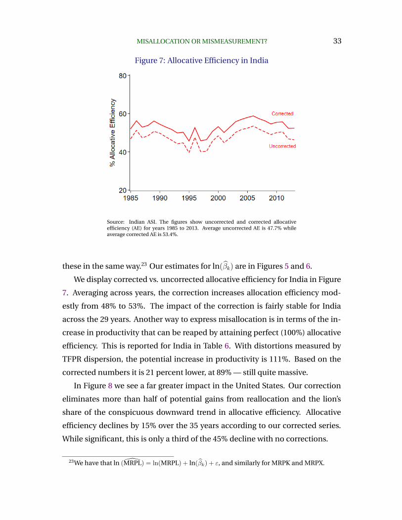
Figure 7: Allocative Efficiency in India
Source: Indian ASI. The figures show uncorrected and corrected allocativeefficiency (AE) for years 1985 to 2013. Average uncorrected AE is 47.7% whileaverage corrected AE is 53.4%.
these in the same way.23 Our estimates for ln(βk) are in Figures 5 and 6.
We display corrected vs. uncorrected allocative efficiency for India in Figure
7. Averaging across years, the correction increases allocation efficiency mod-
estly from 48% to 53%. The impact of the correction is fairly stable for India
across the 29 years. Another way to express misallocation is in terms of the in-
crease in productivity that can be reaped by attaining perfect (100%) allocative
efficiency. This is reported for India in Table 6. With distortions measured by
TFPR dispersion, the potential increase in productivity is 111%. Based on the
corrected numbers it is 21 percent lower, at 89% — still quite massive.
In Figure 8 we see a far greater impact in the United States. Our correction
eliminates more than half of potential gains from reallocation and the lion’s
share of the conspicuous downward trend in allocative efficiency. Allocative
efficiency declines by 15% over the 35 years according to our corrected series.
While significant, this is only a third of the 45% decline with no corrections.
23We have that ln (MRPL) = ln(MRPL) + ln(βk) + ε, and similarly for MRPK and MRPX.
34 BILS, KLENOW, AND RUANE
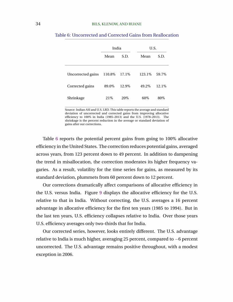
Table 6: Uncorrected and Corrected Gains from Reallocation
India U.S.
Mean S.D. Mean S.D.
Uncorrected gains 110.8% 17.1% 123.1% 59.7%
Corrected gains 89.0% 12.9% 49.2% 12.1%
Shrinkage 21% 20% 60% 80%
Source: Indian ASI and U.S. LRD. This table reports the average and standarddeviation of uncorrected and corrected gains from improving allocativeefficiency to 100% in India (1985–2013) and the U.S. (1978–2013). Theshrinkage is the percent reduction in the average or standard deviation ofgains after our corrections.
Table 6 reports the potential percent gains from going to 100% allocative
efficiency in the United States. The correction reduces potential gains, averaged
across years, from 123 percent down to 49 percent. In addition to dampening
the trend in misallocation, the correction moderates its higher frequency va-
garies. As a result, volatility for the time series for gains, as measured by its
standard deviation, plummets from 60 percent down to 12 percent.
Our corrections dramatically affect comparisons of allocative efficiency in
the U.S. versus India. Figure 9 displays the allocative efficiency for the U.S.
relative to that in India. Without correcting, the U.S. averages a 16 percent
advantage in allocative efficiency for the first ten years (1985 to 1994). But in
the last ten years, U.S. efficiency collapses relative to India. Over those years
U.S. efficiency averages only two-thirds that for India.
Our corrected series, however, looks entirely different. The U.S. advantage
relative to India is much higher, averaging 25 percent, compared to −6 percent
uncorrected. The U.S. advantage remains positive throughout, with a modest
exception in 2006.

MISALLOCATION OR MISMEASUREMENT? 35
Figure 8: Allocative Efficiency in the United States
Source: U.S. LRD. The figures show uncorrected and corrected allocativeefficiency (AE) for years 1978 to 2013. Average uncorrected AE is 47.6% whileaverage corrected AE is 67.4%.
Figure 9: Allocative Efficiency: U.S. relative to India
Sources: Indian ASI and U.S. Census LRD. The figures show uncorrected andcorrected allocative efficiency for the U.S. relative to India for years 1985 to 2013.
36 BILS, KLENOW, AND RUANE
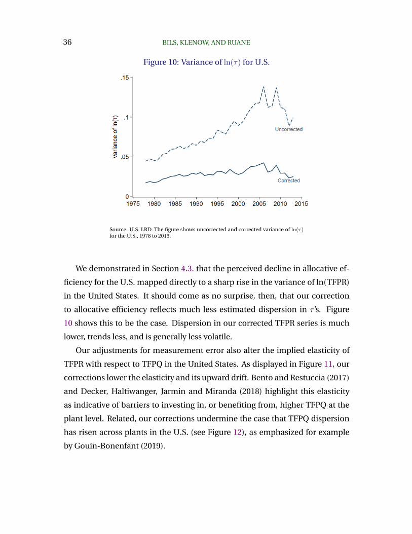
Figure 10: Variance of ln(τ) for U.S.
Source: U.S. LRD. The figure shows uncorrected and corrected variance of ln(τ)for the U.S., 1978 to 2013.
We demonstrated in Section 4.3. that the perceived decline in allocative ef-
ficiency for the U.S. mapped directly to a sharp rise in the variance of ln(TFPR)
in the United States. It should come as no surprise, then, that our correction
to allocative efficiency reflects much less estimated dispersion in τ ’s. Figure
10 shows this to be the case. Dispersion in our corrected TFPR series is much
lower, trends less, and is generally less volatile.
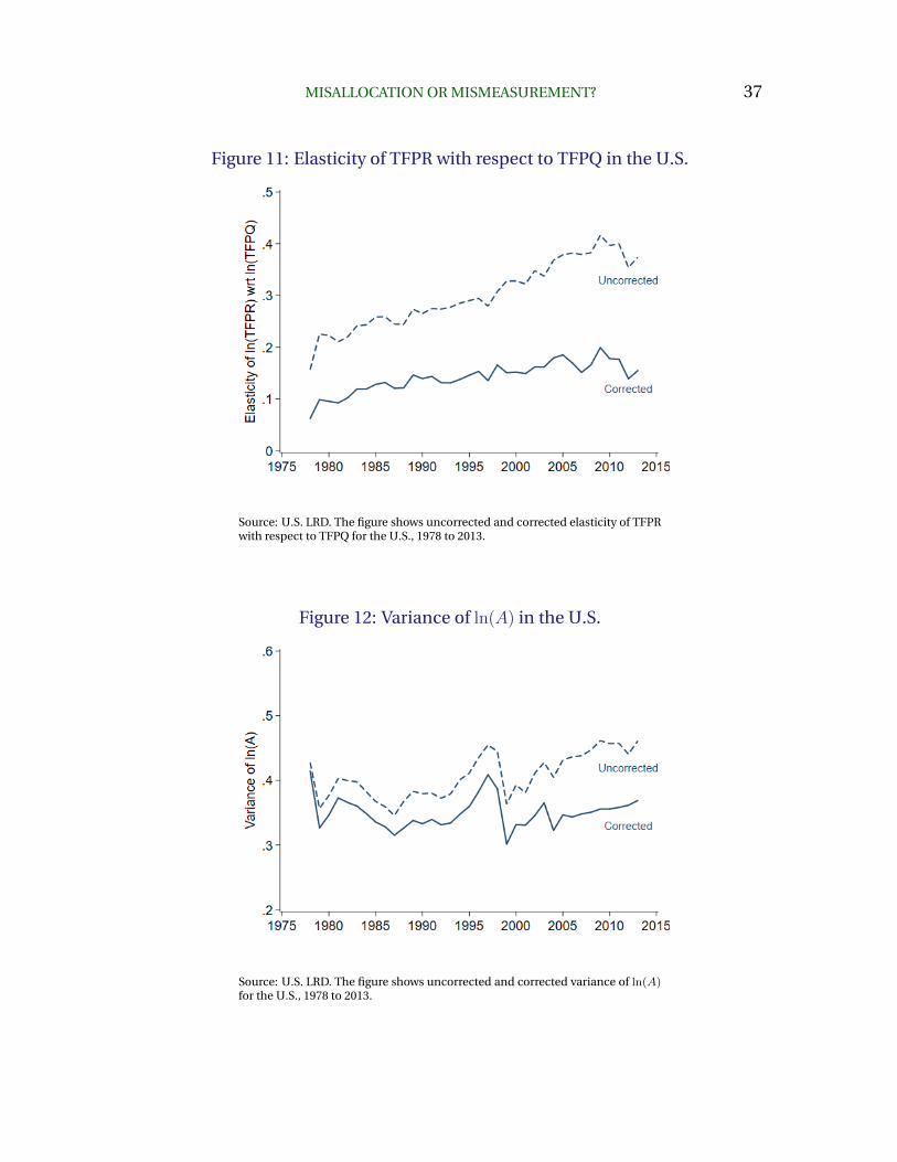
Our adjustments for measurement error also alter the implied elasticity of
TFPR with respect to TFPQ in the United States. As displayed in Figure 11, our
corrections lower the elasticity and its upward drift. Bento and Restuccia (2017)
and Decker, Haltiwanger, Jarmin and Miranda (2018) highlight this elasticity
as indicative of barriers to investing in, or benefiting from, higher TFPQ at the
plant level. Related, our corrections undermine the case that TFPQ dispersion
has risen across plants in the U.S. (see Figure 12), as emphasized for example
by Gouin-Bonenfant (2019).
MISALLOCATION OR MISMEASUREMENT? 37
Figure 11: Elasticity of TFPR with respect to TFPQ in the U.S.
Source: U.S. LRD. The figure shows uncorrected and corrected elasticity of TFPRwith respect to TFPQ for the U.S., 1978 to 2013.
Figure 12: Variance of ln(A) in the U.S.
Source: U.S. LRD. The figure shows uncorrected and corrected variance of ln(A)for the U.S., 1978 to 2013.
38 BILS, KLENOW, AND RUANE
8. Conclusion
We proposed a way to estimate the true dispersion of marginal products across
plants in the presence of additive measurement errors in revenue and inputs.
We showed that the response of revenue growth to input growth should be lower
for high-TFPR plants in the presence of measurement error. And then used the
projection of that response on TFPR to correct for measurement error. While
our method employs several assumptions, we used simulations to demonstrate
that our approach is robust or at least conservative.
We implemented our method on data from the Indian Annual Survey of In-
dustries from 1985–2013 and the US. Annual Survey of Manufacturing from
1978–2013. In India, we estimated that true marginal products were signifi-
cantly less dispersed than average products. As a result, potential gains from
reallocation fell 21% and the volatility of those gains across years fell by 20%.
In the U.S. our correction had even more bite. Average potential gains from
reallocation fell by 60%, while time-series volatility fell by 80%. Our correction
eliminated 2/3 of a severe downward trend in allocative efficiency for the U.S.
Even corrected, allocative efficiency declined by 15% for U.S. manufacturing
over the 35 years. Based on uncorrected data, allocative efficiency was 6% lower
in the U.S. than in India for 1985 to 2013. In contrast, our corrected series
implies consistently higher allocative efficiency in the U.S. than in India.
We hope our method provides a useful diagnostic for measurement errors
that can be applied when researchers have access to panel data on plants and
firms. For example, David and Venkateswaran (2019) and Bai, Jin and Lu (2019)
apply our correction to firm-level data for China.
Our findings leave many open questions for future research. Why did mea-
surement error worsen considerably over time in the U.S.? Why, even after our
corrections, does ample misallocation remain in the U.S. and India? Is this
real or due to some combination of model misspecification and proportional
measurement error? If it is real, can it be traced to specific government policies
or market failures (e.g. markup dispersion or capital/labor market frictions)?
MISALLOCATION OR MISMEASUREMENT? 39
References
Asker, John, Allan Collard-Wexler, and Jan De Loecker, “Dynamic Inputs and Resource
(Mis)Allocation,” Journal of Political Economy, 2014, 122 (5), 1013–1063.
Bai, Yan, Keyu Jin, and Dan Lu, “Misallocation under Trade liberalization,” NBER
working paper 26188, 2019.
Bartelsman, Eric, John Haltiwanger, and Stefano Scarpetta, “Cross-country Differences
in Productivity: The Role of Allocation and Selection,” American Economic Review,
2013, 103 (1), 305–334.
Bento, Pedro and Diego Restuccia, “Misallocation, Establishment Size, and Productiv-
ity,” American Economic Journal: Macroeconomics, 2017, 9 (3), 267–303.
David, Joel M. and Venky Venkateswaran, “The Sources of Capital Misallocation,”
American Economic Review, 2019, 109 (7), 2531–2567.
Decker, Ryan A., John C. Haltiwanger, Ron S. Jarmin, and Javier Miranda, “Changing
Business Dynamism and Productivity: Shocks vs. Responsiveness,” NBER working
paper 24236, January 2018.
Fort, Teresa C. and Shawn D. Klimek, “The Effect of Industry Classification Changes on
U.S. Employment Composition,” 2016.
Gouin-Bonenfant, Emilien, “Productivity Dispersion, Between-Firm Competition and
the Labor Share,” 2019.
Hopenhayn, Hugo A., “Firms, Misallocation, and Aggregate Productivity: A Review,”
Annual Review of Economics, 2014, 6 (1), 735–770.
Hsieh, Chang-Tai and Peter J. Klenow, “Misallocation and Manufacturing TFP in China
and India,” Quarterly Journal of Economics, 2009, 124 (4), 1403–1448.
Redding, Stephen J. and David E. Weinstein, “Measuring Aggregate Price Indices
with Taste Shocks: Theory and Evidence for CES Preferences,” Quarterly Journal of
Economics, 2019, 135 (1), 503–560.

40 BILS, KLENOW, AND RUANE
Restuccia, Diego and Richard Rogerson, “Policy Distortions and Aggregate Productivity
with Heterogeneous Plants,” Review of Economic Dynamics, October 2008, 11, 707–
720.
and , “The Causes and Costs of Misallocation,” Journal of Economic Perspectives,
2017, 31 (3), 151–174.
Rotemberg, Martin and T. Kirk White, “Measuring Cross-Country Differences in Misal-
location.,” 2019.
Syverson, Chad, “What Determines Productivity?,” Journal of Economic literature, 2011,
49 (2), 326–365.
White, T. Kirk, Jerome P. Reiter, and Amil Petrin, “Imputation in U.S. Manufacturing
Data and Its Implications for Productivity Dispersion,” Review of Economics and
Statistics, 2018, 100 (3), 502–509.