Narrowing the Universe: A Machine Learning Approach to ...
47
Chicago-Kent Journal of Intellectual Property Chicago-Kent Journal of Intellectual Property Volume 20 Issue 1 Article 8 7-12-2021 Narrowing the Universe: A Machine Learning Approach to Patent Narrowing the Universe: A Machine Learning Approach to Patent Clearance Clearance Rebecca Weires Joshua Rosefelt Katelyn Meylor Stephanie Shim Lindsay Chong Follow this and additional works at: https://scholarship.kentlaw.iit.edu/ckjip Part of the Law Commons Recommended Citation Recommended Citation Rebecca Weires, Joshua Rosefelt, Katelyn Meylor, Stephanie Shim & Lindsay Chong, Narrowing the Universe: A Machine Learning Approach to Patent Clearance, 20 Chi.-Kent J. Intell. Prop. 180 (2021). Available at: https://scholarship.kentlaw.iit.edu/ckjip/vol20/iss1/11 This Article is brought to you for free and open access by Scholarly Commons @ IIT Chicago-Kent College of Law. It has been accepted for inclusion in Chicago-Kent Journal of Intellectual Property by an authorized editor of Scholarly Commons @ IIT Chicago-Kent College of Law. For more information, please contact [email protected], [email protected].
Transcript of Narrowing the Universe: A Machine Learning Approach to ...

Chicago-Kent Journal of Intellectual Property Chicago-Kent Journal of Intellectual Property
Volume 20 Issue 1 Article 8
7-12-2021
Narrowing the Universe: A Machine Learning Approach to Patent Narrowing the Universe: A Machine Learning Approach to Patent
Clearance Clearance
Rebecca Weires
Joshua Rosefelt
Katelyn Meylor
Stephanie Shim
Lindsay Chong
Follow this and additional works at: https://scholarship.kentlaw.iit.edu/ckjip
Part of the Law Commons
Recommended Citation Recommended Citation Rebecca Weires, Joshua Rosefelt, Katelyn Meylor, Stephanie Shim & Lindsay Chong, Narrowing the Universe: A Machine Learning Approach to Patent Clearance, 20 Chi.-Kent J. Intell. Prop. 180 (2021). Available at: https://scholarship.kentlaw.iit.edu/ckjip/vol20/iss1/11
This Article is brought to you for free and open access by Scholarly Commons @ IIT Chicago-Kent College of Law. It has been accepted for inclusion in Chicago-Kent Journal of Intellectual Property by an authorized editor of Scholarly Commons @ IIT Chicago-Kent College of Law. For more information, please contact [email protected], [email protected].

180
NarrowingtheUniverse:A Machine Learning Approach to Patent Clearance
REBECCA WEIRES, JOSHUA ROSEFELT,
KATELYN MEYLOR, STEPHANIE SHIM, AND LINDSAY CHONG*
* Introducing Rebecca Weires, Litigation Associate, Fish & Richardson P.C.; J.D., Stanford LawSchool, 2020; M.S. Bioengineering, Stanford University, 2020; Joshua Rosefelt, Litigation Associate, Fish & Richardson P.C.; J.D., Stanford Law School, 2020; Katelyn Meylor, B.A. International Relations, Stanford University, expected 2022; Stephanie Shim, B.A. History and East Asian Studies, Stanford University, expected 2021; and Lindsay Chong, B.A. Political Science, Stanford University, expected 2022. We also acknowledge Shawn P. Miller, Lisa Larrimore Ouellette, Reid Whitaker, anonymous peer reviewers, and attendees at the 2019 Stanford NPE Dataset Symposium, for their helpful feedback.

2021 NARROWING THE UNIVERSE 181
ABSTRACT
Companies cannot reliably predict which patents are likely to be asserted against them. If they could, they would be better able to quantify and mitigate their own patent infringement risk. We used machine learning methods, informed by legal scholars’ understanding of relevant patent traits, to improve on prior attempts to predict litigation.
We built primarily on Colleen Chien’s Predicting Patent Litigation. Chien used traits from a patent’s legal history and developed a method of prediction based on the traits acquired before litigation, but not after. She demonstrated that the traits acquired before litigation are useful predictors. Evaluating Chien’s approach, we determined that her logistic regression model was generalizable—that is, not overfit to her training sample—though it does not perform as well on real datasets as her matched-pairs evaluation suggested. We found that year-over-year changes in patenting and litigation will hinder real-world prediction with this approach, but only modestly.
Building a much larger dataset of newer patents, and selecting machine learning models tailored to the task, we improved on Chien’s results. Our random forest model had a 7.8% greater area under the precision-recall curve, and it could allow a company to narrow its patent clearance search to a set of patents up to 34% smaller, compared to Chien’s logistic regression approach. We report our results on a random sample of patents using standardized metrics, providing a baseline for future work predicting patent litigation.

182 CHI.-KENT J. INTELL. PROP. | PTAB BAR ASSOCIATION Vol. 20:1
TABLE OF CONTENTS I. INTRODUCTION: THE “WAIT AND SEE” APPROACH TO PATENT
LITIGATION RISK AND ALTERNATIVES .......................................... 183 II. LITERATURE REVIEW: PRIOR ATTEMPTS TO PREDICT LITIGATION ...... 186 III. METHODS: MACHINE LEARNING WITH RELEVANT TRAITS AND CROSS-
VALIDATION ................................................................................... 190 A. Chien’s “Acquired Traits” Approach ...................................... 191 B. Intrinsic and Acquired Traits in Our Dataset .......................... 191 C. Samples for Training and Validation ...................................... 197 D. Machine Learning Models ...................................................... 199 E. False Positives and Precision-Recall Metric ........................... 206
IV. RESULTS: CHIEN’S APPROACH VALIDATED AND IMPROVEMENTS WITHTHE RANDOM FOREST MODEL ....................................................... 207
V. DISCUSSION: FURTHER WORK COMBINING LEGAL KNOWLEDGE ANDMACHINE LEARNING METHODS ..................................................... 213
VI. CONCLUSION: A STEP FORWARD AND A BASELINE ............................ 218 APPENDIX .................................................................................................. 219

2021 NARROWING THE UNIVERSE 183
I. INTRODUCTION: THE “WAIT AND SEE” APPROACH TO PATENTLITIGATION RISK AND ALTERNATIVES
High-tech companies bear risks and costs because they cannot reliably predict which patents will be asserted against them. Big data and machine learning can help, though few have used them for this problem. We use machine learning to predict which patents will be litigated, building on legal scholars’ and economists’ knowledge of the patent traits associated with litigation. With simple machine learning models, we made a measurable improvement over scholars’ past work. A small company in the high-tech sector could use our models to narrow its patent clearance searches to the universe of patents most likely to be asserted against it.
An emerging company in the high-tech sector faces great uncertainty around patent infringement liability. Over 300,000 utility patents are issued every year,1 and the vast majority are never enforced through litigation.2 How is a small company to know and mitigate its risk? Reviewing every patent related to the company’s technology would be too expensive and time consuming. The company could have tens of thousands of patents to review and would find it unclear whether each patent reads on the company’s product.3 Designing around the thousands of patents4 that may read on the company’s technology might be impossible. Even if the company could find a design-around, it would have to expend tremendous resources and forego promising opportunities just to design around patents that never posed a litigation risk. Exhaustive patent clearance searches, or freedom to operate analyses, have such severe shortcomings that they have not historically been the norm in high-tech as they are in, for example, life sciences.5 Without a
1. U.S. Patent Statistics Summary Table, Calendar Years 1963 to 2019, USPTO,https://www.uspto.gov/web/offices/ac/ido/oeip/taf/us_stat.htm (last visited Jul. 19, 2020).
2. Infra, Part III.B; Mark A. Lemley, Rational Ignorance at the Patent Office, 95 NW. U. L. REV.1495, 1507 (2001) (finding that about 1.5% of all patents are litigated).
3. See Janet Freilich & Jay P. Kesan, Towards Patent Standardization, 30 HARV. J. L. & TECH.233, 239–40 (2017) (describing the lack of standardization in patent terminology, particularly in software, and its effect on notice and disclosure functions of patent law).
4. As an extreme example, RPX found in the early 2010s that 250,000 in-force patents related tosmartphones, Daniel O’Connor, One in Six Active U.S. Patents Pertain to the Smartphone, DISRUPTIVE COMPETITION PROJECT (Oct. 17, 2012), https://www.project-disco.org/intellectual-property/one-in-six-active-u-s-patents-pertain-to-the-smartphone/, and the assets of 30,000 patent holders cover Bluetooth technology alone, Evan Engstrom, So How Many Patents Are in a Smartphone?, ENGINE, https://www.engine.is/news/category/so-how-many-patents-are-in-a-smartphone (last visited Aug. 11, 2020).
5. See Kent Richardson & Erik Oliver, When Strategies Collide: Freedom to Operate vs. Freedomof Action, IP WATCHDOG (Mar. 7, 2019), https://www.ipwatchdog.com/2019/03/07/when-strategies-collide-freedom-to-operate-vs-freedom-of-action/id=107084/.

184 CHI.-KENT J. INTELL. PROP. | PTAB BAR ASSOCIATION Vol. 20:1
reliable way to narrow its focus to the patents most likely to be litigated, the company is instead likely to advise employees not to read or discuss patents.6
Some firms could review competitors’ patenting and litigation activity to narrow their focus, but not this small tech company. While litigation risk in life sciences comes primarily from known competitors, a tech company faces risk not just from its competitors but also from nonpracticing entities (NPEs) or “patent trolls.”7 And while large companies can look to patent assertions by existing NPEs to see what technologies are at risk, a small company is more likely to be a new NPE’s first target.8
The company could try to deter litigation by building a defensive patent portfolio. With enough patents of its own, a company could respond to a patent infringement suit from a competitor with the credible threat of a countersuit. The company could deter litigation from other practicing companies. But defensive portfolios are an expensive solution and ultimately contribute to the patent troll problem. The company would have to spend hundreds of thousands of dollars prosecuting all its patents, and then paying maintenance fees. Even the largest portfolio would not deter nonpracticing entities, who do not make any product or provide any service that could be the subject of an infringement case. And if the company falls on hard times, it may have to sell the patent assets to NPEs, fueling the troll problem.
The company will probably find that the best strategy is a combination approach that may include joining a defensive aggregator and one or more patent pledges, insuring against its risk, rapidly responding to demand letters,
6. See Lisa Larrimore Ouellette, Who Reads Patents?, 35 NATURE BIOTECHNOLOGY 421 (2017)(finding with a survey that 37% of industry researchers in electronics and software had been instructed not to read patents). A further reason companies avoid reading patents is that knowing of the patent can lead to heightened liability for willful patent infringement. See Christopher B. Seaman, Willful Patent Infringement and Enhanced Damages after In Re Seagate: An Empirical Study, 97 IOWA L. REV. 417 (2012) (describing the willfulness requirement for enhanced damages in patent infringement cases, and finding only a small decline in willfulness findings after the Federal Circuit raised the standard for willfulness in In re Seagate).
7. FEDERAL TRADE COMMISSION, PATENT ASSERTION ENTITY ACTIVITY: AN FTC STUDY 128,134 (Oct. 2016) (confirming earlier reports that the vast majority of patents asserted by PAEs relate to computers, communications, and other electronics); James Bessen & Michael J. Meurer, The Direct Costs from NPE Disputes, 99 CORNELL L. REV. 387 (2014) (estimating $29 billion of direct costs from NPE litigation in 2011, falling mostly on small and medium-sized firms).
8. NPEs often target smaller companies first, to test their patents and fund future litigation.Colleen Chien, Startups and Patent Trolls, 17 STAN. TECH. L. REV. 461, 477–78 (2014) (providing survey evidence and anecdotes showing how PAEs use assertions against large companies to “legitimize” their patents and royalty rates when they go after large companies); Bessen & Meurer, supra note 13 (quantifying the costs of NPE litigation for small and medium-sized companies); cf. John R. Allison et al., Patent Quality and Settlement among Repeat Patent Litigants, 99 GEO. L. J. 677, n.11 (2011) (acknowledging this strategy, but finding that many of the most-litigated patents were asserted in parallel against multiple defendants, not in series).

2021 NARROWING THE UNIVERSE 185
and challenging patents before the Patent Trial and Appeal Board (PTAB).9 New aggregators, insurers, pledges, and other organizations have made this combination approach a viable way to reduce risk. Still, costs and uncertainty remain as long as neither the company nor the organizations it joins can anticipate patent assertions.
The company’s combination approach may involve defensive aggregation. Instead of filing its own patent applications, the company could buy patents from other companies before they get into the hands of aggressive asserters. This defensive aggregation approach benefits the company both by deterring threats from practicing companies and by preventing threats from NPEs. The company could act individually or as part of a collective. Defensive patent aggregator organizations like RPX and AST keep patents out of the hands of nonpracticing entities by purchasing them directly.10 Defensive aggregation is an imperfect solution without a reliable way to predict the incidence of patent litigation. The company would inevitably pay, directly or through an organization, to license and acquire patents that would never have been asserted.
If more patents contribute to the problem, eliminating patents could help. Individual companies, along with organizations like Unified Patents and RPX, challenge questionably-valid patents in inter partes review (IPR) at the PTAB to prevent them from being asserted in more costly district court litigation.11 PTAB challenges are likewise an imperfect solution without a reliable way to predict the incidence of patent litigation. IPR petitioners have two choices: challenge patents preemptively or wait until the patents are asserted in demand letters or district court litigation. Taking the first route, petitioners waste resources challenging patents that never would have been asserted. Taking the second route, alleged infringers incur the costs of litigation and settlement, especially if the court refuses to stay litigation.12
A number of insurers cover patent litigation, with products tailored to patent holders or defendants, and some specifically protect against NPE
9. MARTA BELCHER & JOHN CASEY, HACKING THE PATENT SYSTEM: A GUIDE TO ALTERNATIVE PATENT LICENSING FOR INNOVATORS (2016) (summarizing these new approaches as a resource to companies in the high-tech sector).
10. Patent Sales, RPX, https://www.rpxcorp.com/platform/patent-sales/ (last visited Aug. 4, 2020);Interested in Selling to AST?, ALLIED SECURITY TRUST, https://ast.com/sell-to-ast/ (last visited Aug. 4, 2020). 11. Success at Challenging Bad Patents, UNIFIED PATENTS, https://www.unifiedpatents.com/success (last visited Aug. 4, 2020); Patent Quality Initiative, RPX, http://www.rpxcorp.com/platform/patentqualityinitiative/ (last visited Aug. 4, 2020).
12. Forrest McClellen et al., How Increased Stays Pending IPR May Affect Venue Choice, LAW360(Oct. 17, 2012), https://www.law360.com/articles/1220066/how-increased-stays-pending-ipr-may-affect-venue-choice (finding district courts grant about three-quarters of motions for stays pending IPR decisions).

186 CHI.-KENT J. INTELL. PROP. | PTAB BAR ASSOCIATION Vol. 20:1
litigation.13 Insurers that cannot predict which patents create litigation risk may only offer protection against certain known patents.14 Insurance is still mostly a wait-and-see approach—the firm reacts to demand letters and lawsuits, instead of proactively eliminating the chance of litigation.15 IPRs and defensive aggregation, along with patent pledges, can all be part of a combination approach, but each is effective only for a limited set of patents. Overall, even the combination approach cannot be maximally effective without a good way to predict litigation.
II. LITERATURE REVIEW: PRIOR ATTEMPTS TO PREDICT LITIGATION
Attempting to confront these limitations, Professor Colleen Chien builta model in 2011 to predict whether a patent would be litigated.16 Chien’s work, which she introduced in Predicting Patent Litigation, has been cited as a step toward improving certainty about the value of a given patent.17 Chien’s work was an important step toward untangling the causal relationships between litigation and indicators of patent value,18 the scope of
13. Policies Available, INTELLECTUAL PROPERTY INSURANCE, https://patentinsuranceonline.com/policies-available (last visited Aug. 4, 2020); Patent Risk: Now It Can Be Insured, RPX INSURANCE SERVICES, http://www.rpxinsurance.com/ (last visited Aug. 4, 2020); The ANA to Provide Patent Troll Insurance, ANA, https://www.ana.net/content/show/id/36150 (last visited Aug. 4, 2020); Aon Launches Insurance Solution for Intellectual Property Liability, AON, https://aon.mediaroom.com/news-releases?item=137726 (last visited Aug. 4, 2020).
14. See Bernhard Ganglmair et al., The Effect of Patent Litigation Insurance: Theory and Evidencefrom NPEs 3–4 (Sep. 2018) (unpublished manuscript), https://www.ssrn.com/abstract=3279130 (describing IPISC’s NPE defense policy, which covers a closed list of patents).
15. See Alex Butler, Patent Risk Management and Controlling Patent Litigation Costs, IPVISION,http://info.ipvisioninc.com/IPVisions/bid/21987/Patent-Risk-Management-and-Controlling-Patent-Litigation-Costs (last visited Aug. 7, 2020) (data driven IP consulting company advising companies to take a “proactive” approach to NPE litigation by strategizing in the first 48-72 hours after receiving a demand letter); John A. Amster, 3 Things Every Entrepreneur Should Know About Patent Risk, ENTREPRENEUR (Jul. 17, 2014), https://www.entrepreneur.com/article/235689 (advising small companies to be proactive about litigation risk by reacting to assertion letters by learning as much as possible about the asserter, and to directly limit risk with insurance or by preemptively acquiring or licensing patents on the market); but see Ganglmair et al., supra note 20 (finding the existence of patent litigation insurance may deter NPE litigation).
16. Colleen V. Chien, Predicting Patent Litigation, 90 TEX. L. REV. 283, 286–87 (2011).17. Michael J. Burstein, Patent Markets: A Framework for Evaluation, 47 ARIZ. ST. L.J. 507, 529
(2015) (citing Chien alongside the practices of RPX as evidence of how data analytics are used to forecast patent litigation and value); Brian J. Love et al., Determinants of Patent Quality: Evidence from Inter Partes Review Proceedings, 90 U. COLO. L. REV. 67, 79 (2019) (citing Chien’s as one method for assessing the private value of a patent in the absence of direct evidence).
18. See Alberto Galasso et al., Trading and Enforcing Patent Rights, 44 RAND J. ECON. 275, 289(2013) (citing Chien’s finding on the relationship between patent transfer and litigation, and going on to study the causal link between patent transfer and litigation).

2021 NARROWING THE UNIVERSE 187
the patent troll problem,19 and the social benefits of the patent system.20 Her study was useful as a proof of concept but was limited to fewer than two thousand patents, now long expired, and only ten traits.21 We used a larger, newer dataset and more advanced methods to further develop what Chien had envisioned: a tool to whittle an unwieldy body of patents down to a smaller set most relevant to a business.
A few scholars have attempted to model the incidence of patent litigation. Most legal scholars focus on the descriptive, exploring the characteristics of highly-litigated patents and moving toward prediction with simple logistic regression models.22 With small datasets and no cross-validation, this group has yet to yield an accurate and generalizable model, though Chien comes closest. Machine learning experts have developed advanced models to predict patent litigation, including neural network models, clustering models, graph models of citations, and hybrid approaches.23 These approaches focus heavily on natural language processing using the text of patents and citation networks. Their predictive power is limited by the authors’ failure to include traits in the patent’s legal history that are known by legal scholars to correlate with litigation. Economists have employed sophisticated models on larger datasets of relevant traits to isolate the effects of each feature on the likelihood of
19. Brian J. Love, An Empirical Study of Patent Litigation Timing: Could a Patent Term ReductionDecimate Trolls without Harming Innovators, 161 U. PA. L. REV. 1309, 1315 (2013) (citing Chien as one of a handful of studies with divergent findings about the amount of litigation that nonpracticing entities are responsible for).
20. Mark A. Lemley, Faith-Based Intellectual Property, 62 UCLA L. REV. 1328, 1332 (2015)(citing Chien as part of a body of “sophisticated empirical work” that should inform patent policy).
21. Chien, supra note 22, at 309, 315. A dataset this size could be adequate for statistical inference,where larger datasets can lead to statistically significant findings without practical significance. For prediction, bigger is generally better and allows us to use more complex models without overfitting. We do not make claims about causality based on the statistical significance of our outputs.
22. John R. Allison et al., Extreme Value or Trolls on Top? The Characteristics of the Most-Litigated Patents, 158 U. PA. L. REV. 1 (2009) (focusing on descriptive statistics of the most-litigated patents; employing a logistic regression on a dataset of 212 patents and only a handful of traits); Chien, supra note 22.
23. Qi Liu et al., Patent Litigation Prediction: A Convolutional Tensor Factorization Approach,PROC. 27TH INT’L JOINT CONF. ON ARTIFICIAL INTELLIGENCE 5052 (2018) (developing a hybrid neural network and network embedding model to predict which patents will be the subject of litigation between pairs of firms; using a large dataset including the text of the patents, information on the face of the patent, and citations, but not including any traits characterizing the patent owner or the patent’s legal history); P. Wongchaisuwat et al., Predicting Litigation Likelihood and Time to Litigation for Patents, PROC. 16TH INT’L CONF. ON ARTIFICIAL INTELLIGENCE & L. 257 (2017) (using clustering and ensemble methods to predict litigation and time to litigation, using a large dataset including the text of the patent, information on the face of the patent, assignee revenue, and citation networks, but not the patent’s legal history); W M Campbell et al., Predicting and Analyzing Factors in Patent Litigation, 30TH CONF. ON NEURAL INFO. PROCESSING SYS. (2016) (developing a hybrid random forest and logistic regression model to predict litigation, leveraging the citation graph to normalize traits, and using a variety of traits found on the face of the patent).
188 CHI.-KENT J. INTELL. PROP. | PTAB BAR ASSOCIATION Vol. 20:1
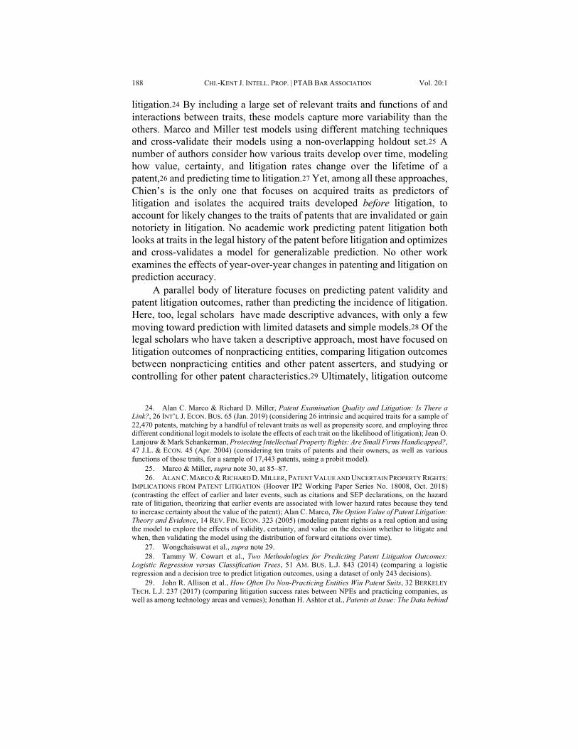
litigation.24 By including a large set of relevant traits and functions of and interactions between traits, these models capture more variability than the others. Marco and Miller test models using different matching techniques and cross-validate their models using a non-overlapping holdout set.25 A number of authors consider how various traits develop over time, modeling how value, certainty, and litigation rates change over the lifetime of a patent,26 and predicting time to litigation.27 Yet, among all these approaches, Chien’s is the only one that focuses on acquired traits as predictors of litigation and isolates the acquired traits developed before litigation, to account for likely changes to the traits of patents that are invalidated or gain notoriety in litigation. No academic work predicting patent litigation both looks at traits in the legal history of the patent before litigation and optimizes and cross-validates a model for generalizable prediction. No other work examines the effects of year-over-year changes in patenting and litigation on prediction accuracy.
A parallel body of literature focuses on predicting patent validity and patent litigation outcomes, rather than predicting the incidence of litigation. Here, too, legal scholars have made descriptive advances, with only a few moving toward prediction with limited datasets and simple models.28 Of the legal scholars who have taken a descriptive approach, most have focused on litigation outcomes of nonpracticing entities, comparing litigation outcomes between nonpracticing entities and other patent asserters, and studying or controlling for other patent characteristics.29 Ultimately, litigation outcome
24. Alan C. Marco & Richard D. Miller, Patent Examination Quality and Litigation: Is There aLink?, 26 INT’L J. ECON. BUS. 65 (Jan. 2019) (considering 26 intrinsic and acquired traits for a sample of 22,470 patents, matching by a handful of relevant traits as well as propensity score, and employing three different conditional logit models to isolate the effects of each trait on the likelihood of litigation); Jean O. Lanjouw & Mark Schankerman, Protecting Intellectual Property Rights: Are Small Firms Handicapped?, 47 J.L. & ECON. 45 (Apr. 2004) (considering ten traits of patents and their owners, as well as various functions of those traits, for a sample of 17,443 patents, using a probit model).
25. Marco & Miller, supra note 30, at 85–87.26. ALAN C. MARCO & RICHARD D. MILLER, PATENT VALUE AND UNCERTAIN PROPERTY RIGHTS:
IMPLICATIONS FROM PATENT LITIGATION (Hoover IP2 Working Paper Series No. 18008, Oct. 2018) (contrasting the effect of earlier and later events, such as citations and SEP declarations, on the hazard rate of litigation, theorizing that earlier events are associated with lower hazard rates because they tend to increase certainty about the value of the patent); Alan C. Marco, The Option Value of Patent Litigation: Theory and Evidence, 14 REV. FIN. ECON. 323 (2005) (modeling patent rights as a real option and using the model to explore the effects of validity, certainty, and value on the decision whether to litigate and when, then validating the model using the distribution of forward citations over time).
27. Wongchaisuwat et al., supra note 29.28. Tammy W. Cowart et al., Two Methodologies for Predicting Patent Litigation Outcomes:
Logistic Regression versus Classification Trees, 51 AM. BUS. L.J. 843 (2014) (comparing a logistic regression and a decision tree to predict litigation outcomes, using a dataset of only 243 decisions).
29. John R. Allison et al., How Often Do Non-Practicing Entities Win Patent Suits, 32 BERKELEYTECH. L.J. 237 (2017) (comparing litigation success rates between NPEs and practicing companies, as well as among technology areas and venues); Jonathan H. Ashtor et al., Patents at Issue: The Data behind

2021 NARROWING THE UNIVERSE 189
modeling is limited by a lack of transparency about settlement outcomes. Economists and computer scientists have taken up the question of predicting validity, modeling validity outcomes in district courts30 and at the federal circuit,31 as well as predicting PTAB petitions32 and institution decisions.33
In addition to these scholarly works, industry players now have access to more and better data on PTAB and district court litigation with which to assess their own risks and costs. Unified Patents provides analytics assessing patent validity, value, and breadth,34 as well as data on PTAB proceedings.35 Lex Machina provides a wealth of data on district court and PTAB outcomes.36 Outside the patent field, scholars and legal analytics companies are developing tools to help companies predict litigation outcomes.37 Others have demonstrated the ability to predict the likelihood of litigation for property and casualty insurance claims.38 Modeling is difficult in some areas of law, due to a lack of large, high-quality datasets.39 But patent litigation is
the Patent Troll Debate, 21 GEO. MASON L. REV. 957 (2014) (comparing litigation success rates between patent assertion entities and other asserters, and examining other characteristics of PAE patents and assertions); Sannu K. Shrestha, Trolls or Market-Makers? An Empirical Analysis of Nonpracticing Entities, 110 COLUM. L. REV. 114, 142–50 (2010) (comparing litigation outcomes of patent infringement cases filed by 51 nonpracticing entities identified in the press with a sample of patents drawn from 500 randomly selected infringement suits); see also Allison et al., supra note 14, at 681–83 (focusing on descriptive statistics of the most-litigated patents and once-litigated patents); Love, supra note 25, at 1342–45 (comparing litigation outcomes for product companies and nonpracticing entities before and after the final three-years from patent expiration).
30. Shawn P. Miller, Where’s the Innovation: An Analysis of the Quantity and Qualities ofAnticipated and Obvious Patents, 18 VA. L.L. & TECH. 59 (2013).
31. Viju Raghupathi et al., Legal Decision Support: Exploring Big Data Analytics Approach toModeling Pharma Patent Validity Cases, 6 IEEE ACCESS 41518 (2018).
32. ALAN C. MARCO ET AL., USPTO, PATENT LITIGATION AND USPTO TRIALS: IMPLICATIONSFOR PATENT EXAMINATION QUALITY (2015).
33. Yuh-Harn Yang et al., Predicting Institution Decisions in Inter Partes Review Proceedings,100 J. PAT. & TRADEMARK OFF. SOC’Y 697 (2019); William Ho et al., Predicting Bad Patents (University of California, Berkeley May 2017); Raghupathi et al., supra note 37.
34. What Is the Difference Between APIX, CITX and BRIX?, UNIFIED PATENTS (Jul. 17, 2020),http://support.unifiedpatents.com/hc/en-us/articles/115001550673. 35. PTAB Case List, UNIFIED PATENTS, https://portal.unifiedpatents.com/ptab/caselist?sort=case_number (last visited Aug. 4, 2020).
36. LEX MACHINA, https://law.lexmachina.com/ (last visited Aug. 4, 2020). 37. E.g., Daniel Martin Katz et al., A General Approach for Predicting the Behavior of the Supreme
Court of the United States, 12 PLOS ONE e0174698 (2017); Charlotte Alexander et al., Using Text Analytics to Predict Litigation Outcomes (2018) (Georgia State University College of Law, Legal Studies Research Paper No. 2018-13), https://papers.ssrn.com/abstract=3230224; Itai Gurari, From Judging Lawyers to Predicting Outcomes, JUDICATA (Feb. 6, 2018), https://blog.judicata.com/from-judging-lawyers-to-predicting-outcomes-f46aedeb8684; Legal Analytics, PREMONITION, https://premonition.ai/legal_analytics/ (last visited Dec. 3, 2019).
38. Mei Najim, Claim Analytics: A Litigation Prediction Case Study, 2018 SAS GLOB. F. PROC.Paper 2504 (2018).
39. Jason Tashea, Algorithms Fall Short in Predicting Litigation Outcomes, A.B.A. J.,http://www.abajournal.com/magazine/article/data_predicting_litigation_outcomes (last visited Dec. 3, 2019).

190 CHI.-KENT J. INTELL. PROP. | PTAB BAR ASSOCIATION Vol. 20:1
a good target for predictive models because the USPTO provides comprehensive patent datasets. Each of the thousands of suits filed each year arises from one or more patents, providing a tractable problem to model. In addition, patent litigation is relatively uniform because it all occurs in federal courts under a single court of appeals, so similar features could predict litigation in across states and perhaps over time.
Here, we used the tools of machine learning to improve on Chien’s work. We first reproduced Chien’s dataset and model in its entirety. We tested for generalizability and measured the model’s performance on a random sample of patents, including later-issued patents. Then, we assembled a larger dataset of newer patents, which we used to train different supervised learning models. By optimizing and cross-validating the models, we found the one that best identified which patents would be litigated in the future. Our supervised learning models, which can account for interactions between traits, outperformed Chien’s model using standard metrics. The metrics we provide can be used as a baseline for further work in this area. Our improvement, along with each step toward better prediction of the incidence and outcomes of litigation, provides better tools for determining and managing patent litigation risk.
III. METHODS: MACHINE LEARNING WITH RELEVANT TRAITS AND CROSS-VALIDATION
We first replicated Chien’s dataset and model, reconstructing her matched-pairs set of patents issued in 1990, with intrinsic traits and acquired traits developed before litigation. We trained a logistic regression model on that data. We then probed the utility of Chien’s model for predicting future litigation. We used tailored test datasets to learn (1) whether the model was overfit to Chien’s training set and therefore not generalizable, (2) whether the matched-pairs sampling scheme inflates the reported accuracy of the model, and (3) to what extent year-over-year changes in patenting limit the ability of a model trained on one year’s litigation to predict the next year’s litigation.
Next, using a larger, unmatched dataset of patents issued in 2000, we trained three standard supervised learning models: A logistic regression, for comparison to Chien; a kernelized support vector machine (SVM) model; and a random forest model. Each is described in detail below. An advantage of the kernelized SVM and random forest models is that they can capture nonlinear relationships between the traits and the likelihood of litigation. To further optimize performance on this task, we tuned the models’

2021 NARROWING THE UNIVERSE 191
hyperparameters—the function inputs that dictate properties of the training process.
A. Chien’s “Acquired Traits” Approach
Chien assessed the value of traits found in the patent’s legal history for predicting the incidence of litigation. She assembled a dataset that was small by machine learning standards today but appropriate for a proof of concept. The dataset included 659 litigated patents issued in 1990, and for each litigated patent, three non-litigated patents matched by technology class, also issued in 1990.40 For each patent, she coded two types of traits: “intrinsic” traits determined at the time the patent issued or shortly after, such as the number of claims, and “acquired” traits that accumulate over the lifetime of the patent, such as the number of times a patent has been assigned.41 Her work was the first to focus on the relationship between acquired characteristics and the likelihood of litigation.42
To simulate the task of predicting future litigation, Chien’s model looked at each patent’s traits as they existed on the eve of litigation.43 For acquired traits, she truncated the data to only include events that occurred before each patent was litigated.44 She then modeled the likelihood of litigation by fitting a logistic regression model to the matched-pairs dataset.45 Using the same matched-pairs set, Chien evaluated the model, estimating it could predict which patents were litigated with a 25% false negative rate and a 20% false positive rate.46
B. Intrinsic and Acquired Traits in Our Dataset
Each patent in our datasets is characterized by eleven traits. Some traits are intrinsic to the patent—they were established by the time the patent issued or shortly after—others are acquired over the life of the patent. These are the same traits Chien studied. We extracted all traits from the LexisNexis TotalPatent One® database,47 except Small Entity, which we obtained from
40. Chien, supra note 22, at 309.41. Chien, supra note 22, at 298–300.42. Chien, supra note 22, at 298–308.43. Chien refers to this as a “time-series” model. Though some of the raw data is indexed by time,
Chien collapses these time-indexed values to simple counts and indicators, then uses the tools of cross-sectional rather than time-series modeling.
44. Chien, supra note 22, at 287.45. Chien, supra note 22, at 314–315.46. Chien, supra note 22, at 316, 320–26.47. LexisNexis TotalPatent OneTM, LEXISNEXIS® IP, https://www.lexisnexisip.com/products/total-
patent-one/ (last visited Jan. 19, 2020).

192 CHI.-KENT J. INTELL. PROP. | PTAB BAR ASSOCIATION Vol. 20:1
the USPTO PatEx dataset.48 Table 1 describes all eleven traits, and the appendix provides more detailed operational definitions.
Table 1. Patent traits included in our dataset
Intrinsic Traits
Trait Description
Claims Number of claims in the patent
Small Entity Whether the patent was issued to a small entity applicant
Family Members Number of foreign and domestic patents linked to one of the same priority documents, including continuations, continuations-in-part, and divisional patents in the patent family
Foreign Counterparts Number of foreign patents linked directly or indirectly to one of the same priority documents
Acquired Traits
Trait Description
Recorded Assignments Number of recorded assignment events, including name changes and security agreements
Recorded Transfer Whether the patent was assigned after it issued
Owner Size Change Change in owner size from small entity to large entity or vice versa
Maintenance Fees Number of maintenance fees paid
Ex Parte Reexamined Ex parte reexamination certificate issued
Collateralized Security interest in the patent recorded
Forward Citations Number of citations to a patent made by subsequent patents
Our definitions of the intrinsic traits matched Chien’s, but we modified the definitions of a few acquired traits so we could extract them automatically and without excessive computation. We modified the operational definition of Recorded Transfer to avoid manually researching each assignment event. We counted as a Recorded Transfer any assignment
48. Patent Examination Research Dataset (Public PAIR), USPTO, https://www.uspto.gov/learning-and-resources/electronic-data-products/patent-examination-research-dataset-public-pair (last visited Jan. 19, 2020).

2021 NARROWING THE UNIVERSE 193
event labeled “assignment of assignor’s interest” (to eliminate events that are merely name changes and security agreements) and recorded after the issue date (to generally but imperfectly eliminate transfers made under pre-existing invention assignment agreements). Because assignee entity size was not recorded with each assignment, we determined Owner Size Change by looking at maintenance fee payments. This was an undercount relative to Chien because it included only those size changes followed by a maintenance fee payment. We considered a patent to be Collateralized if it had an assignment event that contained the text “security”, “release”, or “collateral”. Finally, Chien adjusted Forward Citations by removing those with common inventorship, an adjustment we omitted because of the much greater processing required. Without the adjustment, there was just as large of a difference in the number of citations between litigated and unlitigated patents; thus, we do not believe the adjustment significantly affected model performance.
We also validated our trait definitions by comparing our dataset to Chien’s, as shown in Figure 1. The sample in Figure 1 was a matched-pairs sample as described below.49 We obtained confidence intervals by resampling 659 litigated patents and three matched pairs per litigated patent. The differences between the patents in our dataset and Chien’s are almost all statistically significant, meaning they do not arise just from sampling variability. They may arise from differences in trait definitions and changes to the data source.50 Overall, though, the datasets are similar. In particular, the degree of difference between litigated and unlitigated patents along each trait is similar or larger in our dataset compared to Chien’s, suggesting our logistic regression model could classify patents about as well as hers.
49. Infra Part III.C.50. For example, forward citations from patents issued in the ‘00s may have been added to the
TotalPatent One database between the time Chien queried the database and when we did. For Forward Citations, only the application date for each citing patent was available, so we assumed an 18-month gap between the application date and the date the citing patent number would be added to the forward citation list of the cited patent. The actual gap would have varied substantially for patents filed before the 1999 amendments to the Patent Act, which provided for publication after 18 months. American Inventors Protection Act, Pub L. No. 106-113, § 4501, 113 Stat. 1501, A-561 (1999). For all other traits, we used the event dates in the raw data to separate pre-litigation and post-litigation events, though the event may not have been added to the dataset immediately on the event date. These undocumented changes to the data source over time make it infeasible to perfectly characterize the patent’s record exactly as it existed on the eve of litigation. The better we can separate pre-litigation events from post-litigation events, the more our validation metrics will reflect the model’s actual performance on patents yet to be litigated.

194 CHI.-KENT J. INTELL. PROP. | PTAB BAR ASSOCIATION Vol. 20:1
Figure 1. Traits of patents issued in 1990, acquired over their lifetimes
Note: Descriptive statistics for acquired characteristics developed over the lifetime of the patent (rather than prior to litigation) in our dataset compared to Chien’s. Top: Descriptive statistics for our dataset. n=659 litigated; n=1977 unlitigated, with three unlitigated patents matched to each litigated patent by technology class. Error bars are 95% confidence intervals from resampling out of the population of litigated and unlitigated patents. Bottom: Descriptive statistics for Chien’s dataset. n=659 litigated; n=1977 unlitigated, with three unlitigated patents matched to each litigated patent by technology class.

2021 NARROWING THE UNIVERSE 195
Our dataset includes traits—Recorded Assignments, Recorded Transfer, and Collateralized—that depend upon recording at the patent office. Not all patent owners actually record these transactions,51 so our values are an undercount relative to the true number of assignments, transfers, and collateralizations. We therefore make no claims about the relationship between the actual number of assignments and likelihood of litigation, or actual collateralization and the likelihood of litigation. Despite spotty recording, these traits can be useful predictors. In fact, it could be that patent owners planning to assert valuable patents are more likely to record collateralizations and assignments of those patents, making recorded transactions an even better predictor of litigation.52 Ultimately, the coefficients of the logistic regression model are evidence of how useful the traits are for prediction.53
Figure 2 compares the traits of patents issued in 1990 and 2000, again using the matched-pairs sampling scheme. About 60% more patents were issued in 2000 than in 1990, and there was an even greater difference in the rate of litigation, with around 1.9% of 2000 patents having recorded litigation events compared to just 0.82% of 1990 patents. Compared to patents issued in 1990, patents issued in 2000 were cited, assigned, transferred, and collateralized more. Some of this growth could be attributable to improvements in information systems that allowed for more efficient prior art searching and more efficient patent markets. In addition, many patents issued in 2000 were a product of the dot-com boom of the late 1990s. This explosion of internet-based companies and coincided with a surge in patenting.54 Following the dot-com bust came the rise of the patent assertion entity business model, which helps account for the rise in assignments litigation.55 Surprisingly, the rate of ex parte reexamination did not decline, even as the 2011 America Invents Act introduced inter partes review and other alternatives to reexamination. For a majority of traits, the difference between litigated and unlitigated patents shrank from 1990 to 2000, which could hinder prediction with the 2000 patents.
51. LISA LARRIMORE OUELLETTE & HEIDI WILLIAMS, REFORMING THE PATENT SYSTEM 11 (TheHamilton Project Policy Proposal No. 2020-12, 2020).
52. Recording rates may higher for larger patent owners. 53. Infra Part IV; infra Table A4.54. Patent Statistics Summary, supra note 7.55. Shawn P. Miller, Who’s Suing Us: Decoding Patent Plaintiffs since 2000 with the Stanford
NPE Litigation Dataset, 21 STAN. TECH. L. REV. 235, 261 (2018) (showing a gradual rise in litigation by patent assertion entities, with a peak in 2011, just after patents issued in 1990 expired).

196 CHI.-KENT J. INTELL. PROP. | PTAB BAR ASSOCIATION Vol. 20:1
Figure 2. Traits of patents issued in 2000, compared to 1990
Note: Descriptive statistics for intrinsic and acquired characteristics developed over the lifetime of the patent (rather than prior to litigation) for patents issued in 1990 compared to patents issued in 2000. Top: Descriptive statistics for patents issued in 2000. n=2739 litigated; n=26,948 unlitigated, with eight unlitigated patents matched by technology class to each litigated patent. Bottom: Descriptive statistics for patents issued in 1990. n=739 litigated; n=5912 unlitigated, with eight unlitigated patents matched by technology class to each litigated patent.

2021 NARROWING THE UNIVERSE 197
Finally, as Chien did, we looked only at the acquired traits developed before the patent’s first litigation event and normalized Forward Citations and Assignments by the number of months between issue and litigation. Thus, the model attempts to sort litigated from matched, unlitigated patents on the eve of litigation. A model that classified patents based on any traits developed after litigation would have poor external validity because litigation itself could change many of a patent’s features. For example, the patent could be invalidated in litigation, or it could gain notoriety, increasing the rate of citations. We considered only litigation events before 2011 to replicate Chien’s dataset more faithfully. We used the date of each litigated patent’s earliest litigation event only and used the same date as a cutoff for matched unlitigated patents. For the non-matched datasets, we gave each unlitigated patent the earliest litigation date of a randomly-selected litigated patent.
C. Samples for Training and Validation
We sampled the 1990 and 1991 patents in several ways to probe the fit and utility of the basic logistic regression model. Replicating Chien’s methods, we started by training the model on a matched-pairs set. This training set included 593 randomly-selected litigated patents issued in 1990 and three times as many unlitigated patents matched to the litigated patents by first-listed technology class.56 As Chien did, we first tested this trained model on the same training set. Second, we tested whether this trained model was overfit to the training set by testing the trained model on a separate holdout set of the remaining 148 litigated patents and their matched unlitigated patents. An overfit model would perform significantly better on the training set than on the separate holdout set, while a generalizable model would perform about the same. Third, we tested the same trained model on a completely random sample of 1990 patents. This unmatched test gives a more realistic picture of the model’s utility for patent clearance searches and risk analysis because the matched-pairs sets are unrealistic. The matched-pairs sets have unrealistically low fractions of unlitigated patents. In addition, the distribution of unlitigated patents’ technology classes in the matched-pairs sets is unrepresentative of the population because it is identical to the technology distribution of the litigated patents, even though
56. We used only utility patents, dropping plant and design patents, statutory inventionregistrations, and reexamination certificates. We included continuations, continuations-in-part, divisionals, and reissue patents that were issued in 1990, 1991, or 2000. Patents issued to Ronald Katz were excluded as likely outliers. The few patents that could not be matched by technology class, either because the technology class field was empty or because there were not enough matched pairs available, were excluded.

198 CHI.-KENT J. INTELL. PROP. | PTAB BAR ASSOCIATION Vol. 20:1
the litigation rate is much higher among some technology classes than others. Fourth, we tested the trained model on a random sample of patents issued in 1991. This gives an even more realistic picture of this model’s utility in real world application because a model predicting future litigation will have to be trained on past litigation. With the 1991 patents, we tested whether year-over-year changes in patenting and litigation significantly degrade model performance. Table 2 summarizes the sampling scheme for the 1990 and 1991 patents.
Table 2. Sampling scheme for patents issued in 1990
Stage Sample
Train model Training set of 591 litigated patents issued in 1990, and for each litigated patent, three randomly-selected unlitigated patents in the same technology class57
Replicate Chien’s testing scheme Training set
Test for overfitting Holdout set of the remaining 148 litigated patents, and for each litigated patent, three randomly-selected unlitigated patents in the same technology class, excluding any patents in the training set
Measure the effect of the sampling scheme on accuracy
Random sample of 72,289 patents issued in 199058
Measure the effect of year-over-year changes in patenting on accuracy
Random sample of 65,302 patents issued in 1991
We then trained, developed, and tested machine learning models on a set of 145,744 patents issued in 2000. Here, we disposed of the matched-pairs sampling scheme in favor of a fully random samples. With an automated labeling process, the higher volume of unlitigated patents in the unmatched sample was not a problem. And while undersampling the unlitigated patents could help overcome unbalanced dataset problems, we instead adjusted the relative weight of litigated and unlitigated patents in the training algorithm, as described below. We expected that training and tuning
57. This matches Chien’s sampling scheme. Colleen V. Chien, supra note 23, at 309.58. The 1990 and 1991 random samples had approximately 591 litigated patents, like the matched-
pairs training set, and had more than enough unlitigated patents to detect a significant change in the false positive rate.

2021 NARROWING THE UNIVERSE 199
the model on a random sample of patents would be likely to result in the best performance on a randomly-sampled test set. Further, performance metrics reported on a random sample would be easiest for a user to understand and would reflect a more typical use case for the model than performance on a matched-pairs set.
Table 3. Sampling scheme for patents issued in 2000
Stage Sample
Train 60% of patents issued in 2000, randomly sampled and non-overlapping with the development and test sets
Develop (Tune hyperparameters)
20% of patents issued in 2000, randomly sampled and non-overlapping with the training and test sets
Test 20% of patents issued in 2000, randomly sampled and non-overlapping with the training and development sets
D. Machine Learning Models
We implemented three different models. Each model attempts to classify patents as litigated or unlitigated, essentially drawing a line that best separates litigated from unlitigated patents. Fitting or “training” each model involves feeding the training dataset into a training algorithm to find the line that best separates litigated patents from unlitigated patents. We trained and tested multiple times, tuning hyperparameters along the way. Hyperparameters are inputs that modify the training process, and we tuned them to arrive at the training process that results in the best classification metrics, described below.59 The three models differ in the method used to find the line between litigated and unlitigated patents and in the shape that line can take. We used the scikit learn python package to implement each model.60 Hyperparameters and coefficients of the trained model are provided in the appendix.61
For the 1990 patents, we trained a logistic regression model, following Chien’s methodology.62 For the patents issued in 2000, we used a machine learning approach to find the best model to predict which patents are likely
59. Infra Part III.E.60. Supervised Learning, SCIKIT-LEARN 0.22.1 DOCUMENTATION, https://scikit-
learn.org/stable/supervised_learning.html#supervised-learning (last visited Jul. 28, 2020). 61. Infra, Tables A3–A8.62. Chien, supra note 22, at 329.

200 CHI.-KENT J. INTELL. PROP. | PTAB BAR ASSOCIATION Vol. 20:1
to be litigated. We trained three types of model: logistic regression (for comparison to Chien), kernelized support vector machine (SVM), and random forest.63 Each type of model is described in detail below.
Logistic regression is a basic supervised learning model.64 It finds the best-fitting linear combination of traits and maps it to a logistic function that outputs a probability of litigation.65 The training process, in effect, finds the linear combination of traits that minimizes a function of the aggregate error between the actual classifications (0 or 1, unlitigated or litigated) and the odds according to the model (between 0 and 1).66 Figure 3 shows a basic structure of a logistic regression on a hypothetical dataset. This relatively simple and flexible approach to determine the relationship between a set of traits and a binary outcome serves as a standard model across disciplines. By finding the linear combination of traits, logistic regression provides an easily interpretable representation of the relationship between each predictor and the outcome. However, it also limits the model to drawing a linear boundary between litigated and unlitigated patents.67 Considering Forward Citations, for example, if the likelihood of litigation were low for patents never cited, high for patents cited a few times, and low for patents cited many times, the basic logistic regression would be limited to finding the best-fit linear relationship between cites and likelihood of litigation, missing the actual nonlinear trend.
63. Liu et al., supra note 29 (comparing their tailored model to SVM and logistic regressionbaselines); Cowart et al., supra note 34 (comparing logistic regression and decision trees—related to random forest—for a litigation prediction problem); Campbell et al., supra note 29 (developing a hybrid random forest and logistic regression model).
64. See GIUSEPPE BONACCORSO, MACHINE LEARNING ALGORITHMS 97–103 (2017) (describinglogistic regression in terms of supervised learning); see generally SCOTT W. MENARD, APPLIED LOGISTIC REGRESSION ANALYSIS (Sage Publications 2nd ed. 2002) (providing a detailed description of logistic regression).
65. MENARD, supra note 70, ch. 1.3.66. Id. (explaining the relationship between the actual outcomes and the odds according to the
model, and describing the training process at a high level of generality); BONACCORSO, supra note 70, at 34–38 (describing the mathematics behind maximum likelihood estimation, showing the relationship between likelihood and error).
67. MENARD, supra note 70, ch. 1.3 (describing the linear relationship); STEPHEN MARSLAND,MACHINE LEARNING: AN ALGORITHMIC PERSPECTIVE, ch. ch. 3.4 (2d ed. 2014) (describing the limitations of linear decision boundaries). To account for nonlinearity, we could use various functions of each trait as additional traits. See Lanjouw & Schankerman, supra note 30 (including functions of some traits, such as the number of claims squared). It is also possible to implement a kernelized logistic regression, but the standard logistic regression is linear.

2021 NARROWING THE UNIVERSE 201
Figure 3. Illustration of a logistic regression model
Note: Basic structure of a logistic regression on a hypothetical dataset with just two traits. The model can be used to output a binary classification (green region or white region; litigated or unlitigated) or a score (shades of green; likelihood of litigation).
SVM is another supervised learning algorithm used for classification or regression.68 SVM is an optimal margin classifier, meaning the training process finds the linear boundary that maximizes the distance to the closest examples.69 Figure 4 shows the basic structure of an SVM model on the same hypothetical dataset. The most basic SVM model outputs only a binary classification, but we used a version adapted to output a score corresponding to the likelihood of litigation.70
68. Support Vector Machines, SCIKIT-LEARN 0.22.1 DOCUMENTATION, https://scikit-learn.org/stable/modules/svm.html#kernel-functions (last visited Jan. 18, 2020).
69. MARSLAND, supra note 73, ch. 8.1.70. Support Vector Machines, supra note 74, pt. 1.4.1.2.

202 CHI.-KENT J. INTELL. PROP. | PTAB BAR ASSOCIATION Vol. 20:1
Figure 4. Illustration of a support vector machine model
Note: Basic structure of an SVM model on the same hypothetical dataset. Note how the position of the decision boundary is different because a different method is used to place it.
As with Logistic Regression, the decision boundary of the most basic SVM model is linear.71 To draw a boundary that is a more complex function of the traits, we used a kernel. A kernel implicitly transforms data into a higher-dimensional space, allowing decision boundaries that are nonlinear.72 For example, a polynomial kernel of degree 2 maps the traits to every possible product of two traits,73 such as the products (Reexamined x Collateralized) and (Recorded Assignments)2, which might predict litigation better than the raw trait values. The Gaussian radial basis function kernel we used maps to infinite-dimensional space and thus allows a greater range of
71. See MARSLAND, supra note 73, ch. 8.1.3.72. Id. ch. 8.2.73. Jean-Philippe Vert et al., A Primer on Kernel Methods, in KERNEL METHODS IN
COMPUTATIONAL BIOLOGY, ch. 2.6 (Bernhard Scholkopf et al. eds., 2004). Alternatively, one could include these products as separate traits. However, more complex kernels cannot easily be reproduced this way.

2021 NARROWING THE UNIVERSE 203
nonlinear boundaries.74 Kernel functionality is built into the scikit learn SVM package.75 Figure 5 shows a kernelized SVM model.
Figure 5. Illustration of a kernelized SVM model
Note: Kernelized SVM on the hypothetical dataset. The decision boundary of the kernelized SVM is not constrained to a linear shape, so it can be much more tailored to the data, even with just two traits.
Complex decision boundaries like the one shown in Figure 5 may reflect sampling noise. If a new sample were drawn from the population, it would show the same overall trends, but would not fall exactly along the complex decision boundary shown. Our sampling scheme allowed us to manage this type of overfitting. With a kernel that allows the decision boundary to take a complex shape, overfitting is likely. We identified overfitting by comparing the performance of the algorithm on the training set to its performance on the development set. If the model did a worse job classifying patents in the development set than in the training set, that meant it was overfit to the training set. When the model was overfit, we regularized
74. Id.75. Support Vector Machines, supra note 76.

204 CHI.-KENT J. INTELL. PROP. | PTAB BAR ASSOCIATION Vol. 20:1
it. Regularization smooths the decision boundary.76 Figure 6 shows the effect of regularization on the decision boundary.
Figure 6. Illustration of a kernelized and regularized SVM model
Note: Effect of regularization on a kernelized SVM model. Because of the kernel, the decision boundary is not limited to a straight line, but because of regularization, it has a simple, smooth shape. This means it is more likely to capture general trends in the data without becoming overfit by capturing sampling noise.
Along with the SVM model, we developed a random forest model. The random forest model is a set of decision trees. An individual decision tree classifies patents as litigated or unlitigated by making a series of binary decisions. Each individual tree draws a rough decision boundary that may not be very accurate. However, random forest is an ensemble learning technique: the model’s final prediction is the average of the results of many individual decision trees.77 The decisions of individual trees and of the ensemble are not limited to linear decision boundaries,78 so a kernel is not
76. See generally Prashant Gupta, Regularization in Machine Learning, MEDIUM (Nov. 16, 2017),https://towardsdatascience.com/regularization-in-machine-learning-76441ddcf99a.
77. MARSLAND, supra note 73, ch. 13.3.78. Id. ch. 13.1.1, Figure 13.1 (illustrating decision boundaries of ensemble models that are more
complex than the boundaries of each underlying model).

2021 NARROWING THE UNIVERSE 205
necessary. The training process and overall structure of this decision-tree approach are quite different from the logistic regression and SVM approaches. The random forest model may therefore perform well on datasets that the logistic regression and SVM models perform poorly on. 79 Figure 7 shows the structure of a decision tree and a random forest model.
Figure 7. Illustration of a single decision tree and a random forest model
Note: Basic structure of a random forest model on a hypothetical dataset. Top Left: A single decision tree using two traits, with one litigated patent highlighted. Top right: Decision boundary equivalent to the single decision tree, with the same litigated patent highlighted. Bottom: Ensemble of 3 trees, each attempting to classify the same highlighted patent, and the final prediction based on the three individual classifications.
79. See Rich Caruana & Alexandru Niculescu-Mizil, An Empirical Comparison of SupervisedLearning Algorithms, PROC. 23RD INT’L CONF. ON MACHINE LEARNING 161 (2006) (showing the variability in the performance of various supervised learning models having different structures).

206 CHI.-KENT J. INTELL. PROP. | PTAB BAR ASSOCIATION Vol. 20:1
For the SVM and logistic regression models, we tried weighting litigated patents more heavily than unlitigated patents to manage the imbalance between the two categories. Where a dataset includes many more of one class than the other, the model may have a high accuracy even if it only does a good job identifying the larger class. We can ensure the training process results in correct classification of the less-numerous litigated patents by giving them a heavier weighting in the training process, penalizing decision boundaries that only properly classify unlitigated patents.
We used an iterative development process to find the hyperparameters, including kernel shape, degree of regularization, and class weight, that result in the best-performing model. We started with default hyperparameters in the scikit learn python package. We trained models on the training set, trying different parameter combinations. We then checked their performance on the development set until we found the hyperparameters that maximized model performance on the development set. This approach can lead to a model that is slightly overfit to the development dataset.80 To avoid overstating model performance, we reported our results on the separate test sample.
E. False Positives and Precision-Recall Metric
Our datasets are imbalanced—there are many more of the unlitigated class than the litigated class. A metric for evaluating performance on an imbalanced dataset must not overstate performance of a model that only classifies one class correctly. If our models were only evaluated for their overall accuracy,81 then a model that classified all patents as unlitigated would probably also be the most “accurate.” By classifying all patents as unlitigated, the model would get it right 98% of the time or more. But such a model would be of no help in patent clearance. A good model should identify most of the actually litigated patents (true positives) without mistakenly sweeping in too many unlitigated patents (false positives). A good metric, therefore, should reward true positives and penalize false positives. It should not reward true negatives much or at all because a model that classifies every example as negative has a high true negative rate.
For each of our logistic regression models, we fix the true positive rate (true positives / [true positives + false negatives]) to about 75% and report the false positive rate (false positives / [false positives + true negatives]) for comparison with Chien’s results. Lower false positive rates indicate better performance. A model that randomly classified patents would have a false
80. See MARSLAND, supra note 73, ch. 2.2.1.81. Accuracy = (true positives + true negatives) / total examples tested

2021 NARROWING THE UNIVERSE 207
positive rate around 75%, equal to the true positive rate. We report the performance of the multiple logistic regression both on the same matched-pairs sample we used to train it, as Chien did, and on the other 1990 and 1991 samples.
We also calculate the Precision-Recall Curve (PRC) to give a fuller picture of model performance.82 The false positive rate at one arbitrary true positive rate provides an incomplete picture—at a high true positive rate, a model that is good at classifying edge cases will look better than a model that is good at classifying easy cases, while at a low true positive rate, the reverse may be true. The PRC shows the precision (true positives / [true positives + false positives]) across all values of recall, or true positive rate.83 The area under the curve (AUC) of the PRC is an aggregate measure of how our model predicts the litigated class. A model that randomly classified patents would have an AUC under 0.02, equal to the litigation rate.
For all trials, we resampled at least 40 times to obtain confidence intervals on the false positive rates and AUCs. Precision-recall curves displayed below are from a sample that resulted in approximately median AUC across all curves.
IV. RESULTS: CHIEN’S APPROACH VALIDATED AND IMPROVEMENTS WITHTHE RANDOM FOREST MODEL
As Figure 8 shows, our logistic regression model performed about as well as Chien’s model by the false positive measure. Our model’s median false positive rate was 22.7% compared to Chien’s 21%.84 21% is within the 95% confidence interval for our model, indicating that Chien’s value could be lower due to sampling, and the difference is not statistically significant. A small discrepancy is also unsurprising given the differences between our trait definitions and Chien’s. Our model performed about as well on the
82. See generally Jesse Davis & Mark Goadrich, The Relationship between Precision-Recall andROC Curves, PROC. 23RD INT’L CONF. ON MACHINE LEARNING 233 (2006).
83. The PRC is a close cousin of the more common Receiver Operator Characteristic (ROC) curve,but that the PRC is better suited than the ROC curve for imbalanced datasets. Id. The shape of the ROC curve depends on the true negative rate, so it paints an overly optimistic picture for imbalanced datasets. The ROC curve may look good if the model classifies easy negative cases correctly, even if it does a poor job at the margin. The PRC, on the other hand, does not depend on the true negative rate. Another way to overcome this problem with the ROC curve is to balance the dataset before calculating the curve. See, e.g., Yang et al., supra note 39, at 707–8 (balancing the slightly imbalanced dataset of PTAB institutiondecisions before calculating the ROC curve, and achieving a slightly lower AUC when balanced); Marco& Miller, supra note 30 (calculating the ROC curve on a matched-pairs sample which ensures balance).Because the dataset is heavily imbalanced, we choose the PRC to avoid throwing out a lot of data inbalancing. Our approach is also simpler and resembles the actual model performance on unbalanced setsin the real world.
84. Chien, supra note 22, at 322.

208 CHI.-KENT J. INTELL. PROP. | PTAB BAR ASSOCIATION Vol. 20:1
holdout set as on the training set, with a larger confidence interval attributable to the smaller sample. The similar false positive rate on the separate holdout set shows our logistic regression model was not overfit to the training set, and we can infer that Chien’s was probably not overfit either.
When tested on a completely random sample of 1990 patents, our model performed better than on the matched-pairs samples, with a median false positive rate of 19.3%. The training set had few patents in less-litigated technology areas. Still, the trained model was able to classify patents in the test set, which had more patents in those areas. It may be that patents in less-litigated technology areas have traits similar to unlitigated patents in other technology areas (e.g. few citations, few transfers, few reexaminations) and so are relatively easy to classify.
In order to provide a picture of a logistic regression model’s accuracy in practice, we tested the model on a random sample of 1991 patents. Since a model predicting future litigation would train on past litigation, it was important to measure the impact of year-over-year changes in patenting and litigation on model performance. Our model’s performance on a random sample of 1991 patents was slightly worse than on the random sample of 1990 patents, with a 21.6% false positive rate. We can infer that the model is modestly susceptible to diminished performance by yearly changes in patenting and litigation.
Looking at false positive rates rather than raw numbers reveals a shortcoming. The random samples included many unlitigated patents: about 99% unlitigated compared to 75% in the matched pairs dataset. Therefore, the false positive rate of 19.3% on the 1990 sample represents 13,837 false positives compared to 402 patents in the matched-pairs training set. Testing on the matched-pairs set painted a rosy picture of model performance when in fact the number of false positives would be quite high in practice.85
85. Lee Petherbridge also discusses this issue with Chien’s approach. Lee Petherbridge, OnPredicting Patent Litigation, 90 TEX. L. REV. SEE ALSO 75, 76–80 (2012).

2021 NARROWING THE UNIVERSE 209
Figure 8. Comparison of logistic regression performance on different test sets using false positive rates
Note: Logistic regression model performance on 1990 and 1991 patent datasets listed in Table 2, measured by setting the true positive rate and finding the false positive rate. Bar heights represent number of patents in the predicted positive set if the test set had 659 litigated and 1977 unlitigated patents. Error bars are 95% confidence intervals obtained by repeatedly resampling both the training and test sets. Left to right: Chien’s reported results on her training set; performance on our training set; performance on a holdout set to test for overfitting; performance on a random sample of patents issued in 1990 to test effects of the matched-pairs sampling scheme; performance on a random sample of patents issued in 1991 to test effects of year-over-year changes in patenting and litigation.
Figure 9 shows the performance of the trained logistic regression model on the same four test sets. Again, the model performed comparably on the matched-pairs training set and the matched-pairs holdout set. Both the shape of the PRC curves and the area under the curve were similar. Like the false positive values above, the AUCs were sensitive to resampling of the training and holdout sets. This was especially true for the smaller holdout

210 CHI.-KENT J. INTELL. PROP. | PTAB BAR ASSOCIATION Vol. 20:1
set. The more jagged appearance of that curve was also due to the smaller sample size. There was a dramatic difference between the PRC curve for the matched-pairs samples and for the random samples. With many more unlitigated patents in the dataset, the measured precision was much lower even though the model classified patents in the same way. Again, the random samples showed the more realistic performance of the model, and they should be considered the true baseline performance against which to measure other models.
Figure 9. Comparison of logistic regression performance on different test sets using precision-recall curves
Note: Model performance on 1990 and 1991 patent datasets listed in Table 2, using the precision recall curve. Median area under the curve (AUC) and 95% confidence intervals obtained by repeatedly resampling both the training and test datasets. Curves depicted are from a single resampling in which all four AUCs all fell within 2% of their respective medians.

2021 NARROWING THE UNIVERSE 211
Figure 10 shows the performance of the three machine learning models on the 2000 dataset. Here, the AUC and shape of the curve were sensitive to resampling, but less so because of the larger sample size. All three models produced better AUC on the 2000 patents than the logistic regression on the random sample of 1990 patents. The SVM and random forest models outperformed the basic logistic regression by a modest margin, with the random forest model producing a 7.8% higher AUC.86 At a true positive rate of 75% (as above), the logistic regression model swept in about 23 unlitigated patents (false positives) per litigated patent (true positive), while the random forest and SVM models swept in about 19 and 22 unlitigated patents per litigated patent, respectively. The more notable difference between the models was at a true positive rate of 12%. At this threshold, the logistic regression model narrowed down the body of relevant patents to 2047 patents likely to be litigated, 316 of which were actually litigated. The random forest model narrowed the body of relevant patents to just 1356 patents likely to be litigated, 316 of which were actually litigated. Thus, the random forest model was about one and a half times as effective at weeding out unlitigated patents.
86. SVM averaged 5.2% better AUC (p=3.5e-5 paired, two-sided t-test). Random forest averaged7.8% better AUC (p=6.0e-7 paired, two-sided t-test).

212 CHI.-KENT J. INTELL. PROP. | PTAB BAR ASSOCIATION Vol. 20:1
Figure 10. Performance of different types of models using precision-recall curves
Note: Precision-recall curves for test datasets of patents issued in 2000, as described in Table 3. Median area under the curve (AUC) and 95% confidence intervals obtained by repeatedly resampling both the training and test datasets. Curves depicted are from one resampling event in which the AUCs all fell within 2% of their medians.
The improvement with our method is most dramatic at these lower recall values. However, all models still fall short of the performance a company would need to rely on the model to narrow down the patents they review. To eliminate patents from its search, a company would want to be reasonably confident it would more likely than not go unlitigated. Therefore, future work should aim toward increasing precision at recalls above 0.5.
The coefficients of the logistic regression models tell us, roughly, which traits were most predictive of litigation. Patents with more US family members and fewer foreign family members were more likely to be litigated, as were patents transferred at least once after being issued, but not assigned many times. In Force—whether the patent had expired for failure to pay

2021 NARROWING THE UNIVERSE 213
maintenance fees or because its term ended—was another strong predictor of litigation. Ex parte reexamination is a much weaker predictor for 2000 patents than for 1990 patents, which probably reflects the AIA’s changes to the available post-grant proceedings. See Tables A4 and A6 for a full list of logistic regression coefficients.
V. DISCUSSION: FURTHER WORK COMBINING LEGAL KNOWLEDGE ANDMACHINE LEARNING METHODS
Two elements are essential to effectively predicting patent litigation: patent traits that legal experts know to be associated with litigation, and a method tailored to the predictive task. We used the “acquired” traits from the patent’s legal history that scholars have found to be associated with litigation. Our predictive model combined standard machine learning techniques with Chien’s unique method of truncating the legal history to characterize the patent on the eve of litigation. Truncation improves external validity by mitigating the effects of litigation on the traits themselves. We tested three different machine learning models and tuned their hyperparameters to perform optimally on this task. Our cross-validation, using both a development set for tuning the model and a test set for the final model, mitigated the effect of overfitting to ensure that we did not overstate our models’ performance. While we were not the first to use machine learning for this task, ours is the first work to combine the machine learning approach with a full set of acquired traits developed before litigation. The result: measurable improvement over a prior attempt.
This type of model is useful to predict litigation or inform design-around decisions, but it is not designed to predict which patents will be asserted in demand letters rather than in court.87 Demand-letter patents may have some features in common with litigated patents, but there is virtually no public data on demand letters with which to test this hypothesis. Therefore, we cannot know how well our model would predict demand letters. The performance of our model might also suffer if it were used to inform design-around decisions on a widespread basis. If, based on prior data, a patent appeared likely to be litigated, and then many firms designed around the patent, it could quickly become unlikely to be litigated. The model would not immediately reflect that change.
Future work should incorporate more information about each patent. Our model’s performance was ultimately limited by the small number of
87. FEDERAL TRADE COMMISSION, supra note 13, at 5 (finding in a survey of patent assertionentities that litigation preceded 87% of licenses, but that number was as low as 29% for certain types of PAE).

214 CHI.-KENT J. INTELL. PROP. | PTAB BAR ASSOCIATION Vol. 20:1
patent traits in our dataset. With just these eleven traits, there is simply not enough information to achieve very high precision at a high true positive rate. Many factors that inform or reflect a patent holder’s decision to litigate a particular patent were not represented in our dataset. Fortunately, a wealth of additional data is available. Future work should incorporate those patent traits other scholars have associated with litigation,88 and that practitioners know are relevant to the decision to litigate. For example, Marco and Miller identified events in the patent examination process, such as appeals and examiner interviews, that predict litigation risk.89 Their results also allow us to rule out the importance of other traits, like the number of backward references and the presence of a functional claim.90 The fact that In Force was such a strong predictor in our model and Chien’s suggests other traits that make a patent more difficult or impossible to litigate, such as being partially invalidated in a PTAB proceeding, could be useful to eliminate more patents from the pool.
In addition, future work should make greater use of information about assignees. Lanjouw and Shankerman found traits like the patent owner’s portfolio size and whether the owner is foreign or domestic are significant predictors of litigation.91 Technology area and industry also matter a great deal.92 And as Figure 11 shows, different types of patents are litigated by different types of entity. Figure 11 compares the traits of patents issued in 1990 to the traits of patents issued in 2000, distinguishing among practicing companies, individuals, and patent-assertion entities.93 While a large part of the difference between the top and bottom plots is attributable to differences in trait and entity type definitions, the overall picture is clear: the traits of litigated patents vary by entity type. Patents litigated by individuals look markedly different from patents litigated by practicing companies and patent-assertion entities. That difference has persisted, though the size of the
88. Future work should incorporate the traits found to be the best predictors of litigation in Chien,supra note 22; Marco & Miller, supra note 30; Lanjouw & Schankerman, supra note 30; Allison et al., supra note 28.
89. Marco & Miller, supra note 30.90. Id.91. Lanjouw & Schankerman, supra note 30.92. See Allison et al., supra note 28, at 16–20 (finding the most-litigated patents are from different
technology and industry areas than once-litigated patents). 93. Entity types are from the NPE LITIGATION DATABASE, https://npe.law.stanford.edu/ (last
visited Jan. 19, 2020). For a detailed description of the NPE database and initial findings from it, see Miller, supra note 61. As Miller et al. did, we considered category 8 to be “Practicing Companies,” category 9 to be “Individuals” and categories 1, 4, and 5 to be “Patent Assertion Entities,” Id. at 255, discarding litigation by other types of nonpracticing entity. Only 1971 of the 2739 litigated patents issued in 2000 were included in the NPE database and coded as one of these categories (n=1449 Practicing Company, n=98 Individual; n=424 PAE).

2021 NARROWING THE UNIVERSE 215
differences has shifted in different directions across traits. The distinction among entity types remains useful in predicting patent litigation.
Figure 11. Characteristics of patents litigated by nonpracticing entities and individuals.
Note: Acquired characteristics developed over the lifetime of the patent (rather than prior to litigation) for litigated patents, by type of entity that asserted the patent. Top: Our dataset of patents issued in 2000. n=1449 practicing company; n=98 individual; n=424 patent assertion entity. Bottom: Chien’s dataset of patents issued in 1990. n=490 practicing company; n=117 individual; n=59 patent assertion entity.
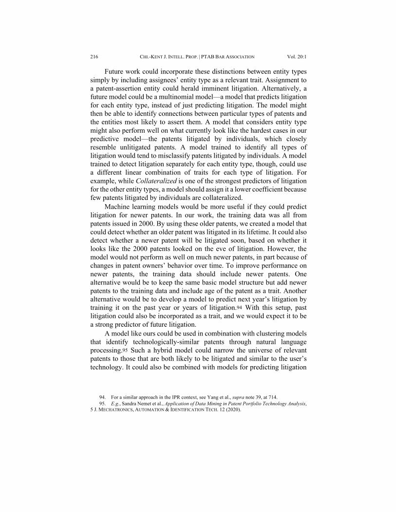
216 CHI.-KENT J. INTELL. PROP. | PTAB BAR ASSOCIATION Vol. 20:1
Future work could incorporate these distinctions between entity types simply by including assignees’ entity type as a relevant trait. Assignment to a patent-assertion entity could herald imminent litigation. Alternatively, a future model could be a multinomial model—a model that predicts litigation for each entity type, instead of just predicting litigation. The model might then be able to identify connections between particular types of patents and the entities most likely to assert them. A model that considers entity type might also perform well on what currently look like the hardest cases in our predictive model—the patents litigated by individuals, which closely resemble unlitigated patents. A model trained to identify all types of litigation would tend to misclassify patents litigated by individuals. A model trained to detect litigation separately for each entity type, though, could use a different linear combination of traits for each type of litigation. For example, while Collateralized is one of the strongest predictors of litigation for the other entity types, a model should assign it a lower coefficient because few patents litigated by individuals are collateralized.
Machine learning models would be more useful if they could predict litigation for newer patents. In our work, the training data was all from patents issued in 2000. By using these older patents, we created a model that could detect whether an older patent was litigated in its lifetime. It could also detect whether a newer patent will be litigated soon, based on whether it looks like the 2000 patents looked on the eve of litigation. However, the model would not perform as well on much newer patents, in part because of changes in patent owners’ behavior over time. To improve performance on newer patents, the training data should include newer patents. One alternative would be to keep the same basic model structure but add newer patents to the training data and include age of the patent as a trait. Another alternative would be to develop a model to predict next year’s litigation by training it on the past year or years of litigation.94 With this setup, past litigation could also be incorporated as a trait, and we would expect it to be a strong predictor of future litigation.
A model like ours could be used in combination with clustering models that identify technologically-similar patents through natural language processing.95 Such a hybrid model could narrow the universe of relevant patents to those that are both likely to be litigated and similar to the user’s technology. It could also be combined with models for predicting litigation
94. For a similar approach in the IPR context, see Yang et al., supra note 39, at 714.95. E.g., Sandra Nemet et al., Application of Data Mining in Patent Portfolio Technology Analysis,
5 J. MECHATRONICS, AUTOMATION & IDENTIFICATION TECH. 12 (2020).

2021 NARROWING THE UNIVERSE 217
outcomes and costs to provide a prediction of which patents pose the highest monetary risk.
With a move to more complex models, attention must be paid to interpretability. Users will be more trusting of a model knowing the factors on which the model based its prediction. Users may want to extract rules of thumb to estimate the litigation potential of any particular patent. An easy solution is to continue to use a linear model, like logistic regression. The coefficients for each trait in the dataset roughly correspond to the importance of the trait for prediction. But other, post-hoc interpretability methods can do a better job of actually capturing and interpreting how the more complex model reaches its decision. For example, the Local Interpretable Model-Agnostic Explanation (LIME) algorithm works by testing the model on both the patent of interest and on similar, artificial examples with slight adjustments to their traits.96 By looking at the change in the model output from each of these small deviations, a picture of the relative salience of each trait emerges. LIME finds a simple model—a linear decision boundary or single decision tree—that approximates the complex model’s nonlinear decision boundary near the patent of interest.
Our results are baseline performance metrics for all this future work. Like our model, future models should be tested on a random sample of patents in a holdout set. Compared to tests using matched-pairs samples, our approach is simple to replicate. Even models trained on matched-pairs sets can be tested on a random sample to get an idea of real-world performance and for comparison to our baseline. We evaluated our models using the precision-recall curve, which is a standard, comprehensive metric appropriate for unbalanced datasets. This will be an appropriate metric for much of the other work in this area.
The metrics we have used can also show whether this type of modeling works better for some types of patents than others. For example, the set of traits we have investigated may be more predictive of litigation for one technology area than another. In pharmaceuticals, where litigation is generally between practicing entities, FDA-related events like the owner listing a patent in the Orange Book might be strong predictors of litigation, though those traits would be irrelevant for high-tech patents. A model trained and tested on one technology area, with a tailored set of traits, can still be
96. Marco Tulio Ribeiro et al., “Why Should I Trust You?”: Explaining the Predictions of AnyClassifier, PROC. 22ND ACM SIGKDD INT’L CONF. ON KNOWLEDGE DISCOVERY & DATA MINING 1135 (2016).

218 CHI.-KENT J. INTELL. PROP. | PTAB BAR ASSOCIATION Vol. 20:1
evaluated with the precision-recall curve.97 A higher AUC would show the model outperforms ours for the particular subset of patents; a lower AUC would show the opposite.
A measure of calibration would be a helpful complement to the PRC. Ultimately, even with more patent traits and a future-focused algorithm, the model will not perfectly predict future litigation. It will not account for whether an infringing product exists. Nor will it account for the dynamics between individual companies that spark litigation and drive decisions about which patent to assert. Instead of outputting a bare classification, the model could predict the likelihood of litigation, and a measure of calibration would indicate to the user whether the likelihoods are correct.
VI. CONCLUSION: A STEP FORWARD AND A BASELINE
By bringing the basic machine learning approach of model tuning and cross-validation into legal scholarship, we have improved on a prior attempt to predict patent litigation. Our performance metrics can serve as a baseline for future attempts. While additional work is needed to expand the dataset and tailor the model to potential users’ needs, we show that our approach of bringing together machine learning and legal knowledge is promising.
Our improvement is a step toward informed patent clearance where it has previously been infeasible. By narrowing the universe of patents to those most likely to be litigated, a company can complete its review at a lower cost. Without good predictions, the company is left to choose between designing around a large body of patents or arbitrarily choosing some patents to read and design around while accepting litigation risk from others. With good predictions, however, the company could reduce its risk by designing around a few patents most likely to be litigated. These predictions can also help defensive aggregators and IPR petitioners better target their efforts. Predicting patent litigation is a critical component of a data-driven approach to preventing patent litigation.
97. A smaller sample size would not affect the expected value of the AUC, so the AUC could bedirectly compared to ours. The AUC would be more sensitive to sampling effects. See supra Figure 9 and text accompanying Figure 9.
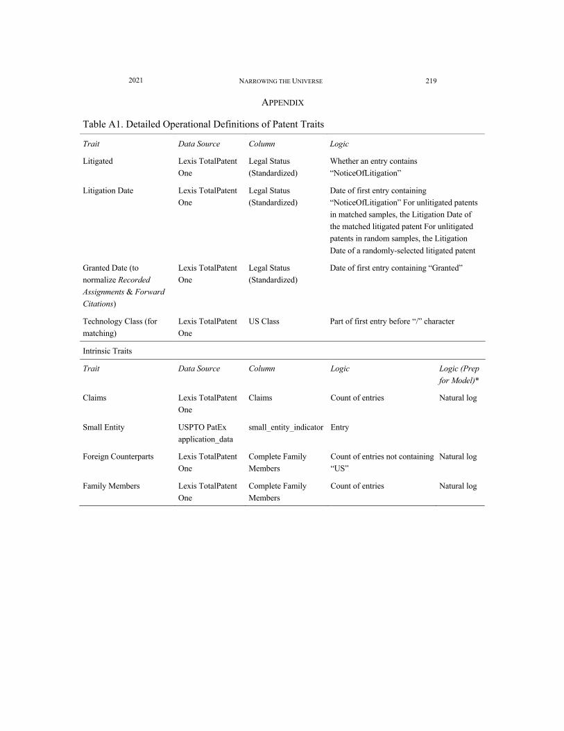
2021 NARROWING THE UNIVERSE 219
APPENDIX
Table A1. Detailed Operational Definitions of Patent Traits
Trait Data Source Column Logic
Litigated Lexis TotalPatent One
Legal Status (Standardized)
Whether an entry contains “NoticeOfLitigation”
Litigation Date Lexis TotalPatent One
Legal Status (Standardized)
Date of first entry containing “NoticeOfLitigation” For unlitigated patents in matched samples, the Litigation Date of the matched litigated patent For unlitigated patents in random samples, the Litigation Date of a randomly-selected litigated patent
Granted Date (to normalize Recorded Assignments & Forward Citations)
Lexis TotalPatent One
Legal Status (Standardized)
Date of first entry containing “Granted”
Technology Class (for matching)
Lexis TotalPatent One
US Class Part of first entry before “/” character
Intrinsic Traits
Trait Data Source Column Logic Logic (Prep for Model)*
Claims Lexis TotalPatent One
Claims Count of entries Natural log
Small Entity USPTO PatEx application_data
small_entity_indicator Entry
Foreign Counterparts Lexis TotalPatent One
Complete Family Members
Count of entries not containing “US”
Natural log
Family Members Lexis TotalPatent One
Complete Family Members
Count of entries Natural log

220 CHI.-KENT J. INTELL. PROP. | PTAB BAR ASSOCIATION Vol. 20:1
Acquired Traits Trait Data
Source Column Logic Logic (Only Events
Before Litigation) Logic (Prep for Model)*
Recorded Assignments
Lexis TotalPatent One
Legal Status (INPADOC)
Count of entries containing “, AS,”
With dates before Litigation Date, divided by months between Granted Date and Litigation Date;
Remove negative values; natural log
Recorded Transfer
Lexis TotalPatent One
Legal Status (INPADOC)
Whether there is an entry containing “ASSIGNMENT OF ASSIGNORS INTEREST” with date after Granted Date
With date before Litigation Date
Owner Size Change
Lexis TotalPatent One
Legal Status (Standardized)
If Small Entity, whether there is an entry containing “Fee Paid” and “M1.” If not Small Entity, whether there is an entry containing “Fee Paid” and “M2.”
With date before Litigation Date
Maintenance Fees
Lexis TotalPatent One
Legal Status (Standardized)
Count of entries containing “Fee Paid” and not containing “EXPX”
With date before Litigation Date
In Force Lexis TotalPatent One
Legal Status (Standardized)
Whether there is an entry containing “Patent Expired”
With date before Litigation Date
Ex Parte Reexamined
Lexis TotalPatent One
Legal Status (INPADOC)
Whether there is an entry containing “, B1,” “, B2,” or “, B3,”
With date before Litigation Date
Collateral-ized
Lexis TotalPatent One
Legal Status (INPADOC)
Whether there is an entry containing both “, AS,” and “SECUR”, “RELEASE”, or “COLLATERAL” in description of assignment type (not just in the name of assignor or assignee)
With date before Litigation Date
Forward Citations
Lexis TotalPatent One
Forward Patent Citations
Count of entries With dates at least 18 months before Litigation Date, divided by months between Granted Date and Litigation Date
Remove negative values; natural log
*All traits of patents issued in 2000 were normalized to a mean of 0 and standard deviation of 1 prior to training. Whenreplicating Chien’s model with 1990 patents, we did not normalize the inputs. Normalization should not affectperformance of a logistic regression model, though it does affect the interpretation of logistic regression coefficients.

2021 NARROWING THE UNIVERSE 221
Table A2. Descriptive Statistics of 1990 and 2000 Patent Datasets
1990 2000 Litigated Unlitigated Litigated Unlitigated n=739 n=5912 n=2739 n=26948
Intrinsic traits Claims 18.0365 12.4849 37.7331 30.9479 Small Entity 0.3599 0.3408 0.35853 0.3101 Family Members 13.3342 8.4076 8.9763 6.2417 Foreign Counterparts 11.1894 6.9503 7.2782 4.9578 Acquired Traits, Developed Prior to Litigation
Recorded Assignments (per month) 0.0159 0.0103 1.6523 0.1885 Recorded Transfer 0.3735 0.1609 0.3118 0.1388 Owner Size Change 0.1827 0.0350 0.0891 0.0260 Maintenance Fees 2.3694 1.5536 1.1661 0.9128 In Force at Time of Litigation 0.9405 0.5179 0.9792 0.8389 Ex Parte Reexamined 0.0325 0.0022 0.0095 0.0007 Collateralized 0.2003 0.0609 0.1446 0.0806 Forward Citations (per month) 0.3954 0.1455 18.8684 1.2104 Acquired Traits, Developed over Patent’s Lifetime Recorded Assignments 3.5859 1.8440 5.2709 2.8570 Recorded Transfer 0.4790 0.1940 0.5469 0.2797 Owner Size Change 0.1894 0.0355 0.1347 0.0439 Maintenance Fees 2.8051 1.7706 2.7192 2.0554 Ex Parte Reexamined 0.0744 0.0027 0.0876 0.0015 Collateralized 0.2869 0.0836 0.3081 0.1503 Forward Citations 107.1367 38.2140 137.7006 70.9933 Note: Descriptive statistics of datasets created using matched pairs sampling, with eight unlitigated patents matched to each litigated patent by technology class. Mean values shown.

222 CHI.-KENT J. INTELL. PROP. | PTAB BAR ASSOCIATION Vol. 20:1
Table A3. Logistic Regression Hyperparameters for Patents Issued in 1990 Parameter Value Reasoning C 1 Default class_weight None Default dual FALSE Default fit_intercept TRUE Default intercept_scaling 1 Default l1_ratio None Default max_iter 100 Default multi_class ‘auto’ Default n_jobs None Default penalty None Approximate default behavior in R random_state 0 Replicability solver ‘newton-cg’ Approximate default behavior in R tol 0.0001 Default verbose 0 Default warm-start FALSE Default Note: Hyperparameters for model sklearn.linear_model.LogisticRegression(), trained on patents issued in 1990.
Table A4. Logistic Regression Coefficients for Patents Issued in 1990 Trait Coefficient Intercept -4.8475Claims 0.2673 Family members 0.8602 Foreign counterpart -0.7708Owner size change 0.8616 Maintenance fees 0.2524 Recorded assignments -7.6827Recorded transfer 0.3889 Collateralized 0.5928 Ex parte reexamined 13.8993 Forward citations 2.6264 In force at time of litigation 1.9090 Small entity 0.6967 Note: Coefficients of trained model sklearn.linear_model.LogisticRegression(), using hyperparameters in Table A3, trained on patents issued in 1990.

2021 NARROWING THE UNIVERSE 223
Table A5. Logistic Regression Hyperparameters for Patents Issued in 2000 Parameter Value Reasoning C 1 Default class_weight {0: 1, 1 : 1} Default dual FALSE Default fit_intercept TRUE Default intercept_scaling 1 Default l1_ratio None Default max_iter 100 Default multi_class ‘auto’ Default n_jobs None Default penalty none Approximate default behavior in R random_state 0 Replicability solver ‘newton-cg’ Approximate default behavior in R tol 0.0001 Default verbose 0 Default warm-start FALSE Default Note: Hyperparameters for model sklearn.linear_model.LogisticRegression(), trained on patents issued in 2000.
Table A6. Logistic Regression Coefficients for Patents Issued in 2000 Trait Coefficient Intercept -4.5197Claims 0.2350 Family members 0.7378 Foreign counterpart -0.7740Owner size change 0.1147 Maintenance fees 0.1665 Recorded assignments -0.1782Recorded transfer 0.3283 Collateralized 0.0682 Ex parte reexamined 0.0683 Forward citations 0.5031 In force at time of litigation 0.6516 Small entity 0.3778 Note: Coefficients of trained model sklearn.linear_model.LogisticRegression(), using hyperparameters in Table A5, trained on patents issued in 2000. Use caution when comparing to Table A4 because data was normalized for this model but was not for the 1990 model.

224 CHI.-KENT J. INTELL. PROP. | PTAB BAR ASSOCIATION Vol. 20:1
Table A7. Support Vector Machine Hyperparameters Parameter Value Reasoning C 0.78 Regularization, optimized experimentally break_ties FALSE Default cache_size 1500 Speed up training class_weight {0: 0.0588, 1: 1} Class imbalance coef0 0.0 Default, ignored because kernel=rbf decision_function_shape ‘ovr’ Default, ignored for binary classification degree 3 Default, ignored because kernel=rbf
gamma 0.028 Kernel parameter, optimized experimentally
kernel ‘rbf’ Flexible, general-purpose kernel max_iter -1 Default probability TRUE Enable precision-recall curve calculation random_state 0 Replicability shrinking TRUE Default tol 0.001 Default verbose FALSE Default Note: Hyperparameters for model sklearn.svm.SVC(), trained on patents issued in 2000.
Table A8. Random Forest Model Hyperparameters Parameter Value Reasoning bootstrap TRUE Default ccp_alpha 0.0 Default class_weight {0: 1, 1: 1} Default, optimized experimentally criterion ‘entropy’ Optimized experimentally max_depth None Default max_features ‘auto’ Default, optimized experimentally max_leaf_nodes None Default max_samples None Default min_impurity_decrease 0.0 Default min_impurity_split None Default min_samples_leaf 42 Regularization, optimized experimentally min_samples_split 2 Default, optimized experimentally min_weight_fraction_leaf 0.0 Default n_estimators 5000 Replicability n_jobs None Default Note: Hyperparameters for model sklearn.ensemble.RandomForestClassifier(), trained on patents issued in 2000.

2021 NARROWING THE UNIVERSE 225