Multi-patch and multi-group epidemic models: a new...

J. Math. Biol.DOI 10.1007/s00285-017-1191-9 Mathematical Biology

Multi-patch and multi-group epidemic models: a newframework

Derdei Bichara1 · Abderrahman Iggidr2

Received: 10 March 2017 / Revised: 26 October 2017© Springer-Verlag GmbH Germany, part of Springer Nature 2017

Abstract Wedevelop amulti-patch andmulti-groupmodel that captures the dynamicsof an infectious disease when the host is structured into an arbitrary number of groupsand interacts into an arbitrary number of patches where the infection takes place. Inthis framework, we model host mobility that depends on its epidemiological status,by a Lagrangian approach. This framework is applied to a general SEIRS model andthe basic reproduction number R0 is derived. The effects of heterogeneity in groups,patches and mobility patterns onR0 and disease prevalence are explored. Our resultsshow that for a fixed number of groups, the basic reproduction number increases withrespect to the number of patches and the host mobility patterns. Moreover, when themobilitymatrix of susceptible individuals is of rankone, the basic reproduction numberis explicitly determined and was found to be independent of the latter if the matrix isalso stochastic. The cases where mobility matrices are of rank one capture importantmodeling scenarios. Additionally, we study the global analysis of equilibria for somespecial cases. Numerical simulations are carried out to showcase the ramifications ofmobility pattern matrices on disease prevalence and basic reproduction number.

Keywords Multi-patch · Multi-group · Mobility · Heterogeneity · Residence times ·Global stability

Mathematics Subject Classification 92D25 · 92D30

B Derdei [email protected]

1 Department of Mathematics and Center for Computational and Applied Mathematics, CaliforniaState University, Fullerton, CA 92831, USA

2 Inria, Université de Lorraine, CNRS, Institut Elie Cartan de Lorraine, UMR 7502, ISGMP Bat. A,Ile du Saulcy, 57045 Metz Cedex 01, France

123

http://crossmark.crossref.org/dialog/?doi=10.1007/s00285-017-1191-9&domain=pdf

http://orcid.org/0000-0002-2210-9360

D. Bichara, A. Iggidr

1 Introduction

The role of heterogeneity in populations and their mobility have long been recognizedas driving forces in the spread of infectious diseases (Anderson andMay 1991;Dushoffand Levin 1995; Prothero 1977; Sattenspiel and Simon 1988). Indeed, populations arecomposed of individuals with different immunological features and hence differ inhow they can transmit or acquire an infection at a given time. These differences couldresult from demographic, host genetic or socio-economic factors (Anderson and May1991). Populations alsomove across different geographical landscapes, importing theirdisease history with them either by infecting or getting infected in the host/visitinglocation.

While the concept of modeling epidemiological heterogeneity within a populationgoes back to Kermack andMcKendrick inmodeling the age of infection (Kermack andMcKendrick 1927), the approach gained prominence with Yorke and Lajmonivich’sseminal paper (Lajmanovich and Yorke 1976) on the spread of gonorrhea, a sexuallytransmitted disease. An abundant and varied literature have followed on understandingthe effects of “superspreaders ” which are core groups on the disease dynamics (Blytheand Castillo-Chavez 1989; Castillo-Chavez and Busenberg 1991; Jacquez et al. 1988,1996; Yorke et al. 1978) or related multi-group models (Bonzi et al. 2011; Fall et al.2007; Hethcote and Thieme 1985; Huang et al. 1992; Nold 1980; Rushton and Maut-ner 1955; Sattenspiel and Simon 1988) (and the references therein). Similarly, spatialheterogeneity in epidemiologyhas been extensively explored in different settings.Con-tinuum models of dispersal have been investigated through diffusion equations (Metzand Diekmann 2014) whereas islandsmodels have been dealt through metapopulationapproach (Arino 2009; Arino and Portet 2015; Arino and Driessche 2006; Iggidr et al.2012, 2016; Salmani and Driessche 2006; Sattenspiel and Dietz 1995), defined hereas continuous models with discrete dispersal.

Although the importance and the complete or partial analysis of these two typesof heterogeneities have been studied separately in the aforementioned papers, lit-tle attention has been given to the simultaneous consideration of groups and spacialheterogeneities. Moreover, previous studies on multi-group rely on differential sus-ceptibility in each group through the WAIFW [Who Acquires Infection From Whom(Anderson and May 1991)] matrices which, we argue, are difficult to quantify. Sim-ilarly, in metapopulation (Eulerian) settings, the movement of individuals betweenpatches is captured in terms of flux of population, making it nearly impossible to trackthe life-history of individuals after the interpatch mixing.

In this paper, we introduce a general modeling framework that structures popula-tions into an arbitrary number of groups (e.g. demographic, ethnic or socio-economicgrouping). These populations, with different health statuses, spend certain amounts oftime in an arbitrary number of locations, or patches, where they could get infected orinfect others. Each patch is defined by a particular risk of infection tied to environmen-tal conditions of each patch. This approach allows us to track individuals of each groupover time and to avoid the use of differential susceptibility of individuals or groups,which is theoretically nice but practically difficult to assess. The likelihood of infec-tion depends both on the time one spends (in a particular patch) and the risk associatedwith that patch. Moreover, we incorporate individuals’ behavioral decisions through

123

Multi-patch and multi-group epidemic models: a new…

differential residence times. Indeed, individuals of the same group spend differentamounts of time in different areas depending on their epidemiological conditions. Wealso considered two cases of the general framework, that are particularly importantfrom modeling standpoint: when the susceptible and/or infected individuals of differ-ent groups have proportional residence times in different patches. That is, when themobility matrix of susceptible (or infected) individuals, M (or P) is of rank one. Inthese cases, we obtain explicit expressions of the basic reproduction number in termsof mobility patterns. It turns out that if M is of rank one and stochastic, the basicreproduction number is independent of the mobility patterns of susceptible host.

In short, we address how group heterogeneity, or groupness, patch heterogeneity,or patchiness, mobility patterns and behavior each alter or mitigate disease dynamics.In this sense, our paper is a direct extension of Bichara and Castillo-Chavez (2016);Bichara et al. (2015, 2016) and Castillo-Chavez et al. (2016) but also other studiesthat capture dispersal through Lagrangian approaches—in which it is possible to trackhost movement after the interpatch mixing—(Cosner et al. 2009; Iggidr et al. 2016;Rodríguez and Torres-Sorando 2001; Ruktanonchai et al. 2016) and a recent paper(Falcón-Lezama et al. 2016) that investigates the effects of daily movements in thecontext of Dengue.

The paper is organized as follows. Section 2 explains themodel derivation, states thebasic properties and the computation of the basic reproduction numberR0(u, v) for ugroups and v patches. Section 3 investigates the role of patch and group heterogeneityon the basic reproduction number, and how dispersal patterns alter R0(u, v) and thedisease prevalence. Section 5 is devoted to the existence, uniqueness and stabilityof equilibria for the considered system under certain conditions. Finally, Sect. 6 isdedicated to concluding remarks and discussions.

2 Derivation of the model

Weconsider a population that is structured in an arbitrarliymanyu groups interacting inv patches.We consider a typical disease captured by an SEIRS structure. Naturally, Si ,Ei , Ii and Ri are the susceptible, latent, infectious and recovered individuals of Groupi respectively. The population of each group is denoted by Ni = Si + Ei + Ii + Ri ,for i = 1, . . . , u. Individuals of Group i spend on average some time in Patch j ,j = 1, . . . , v. The susceptible, latent, infected and recovered populations of group ispendmi j ,ni j , pi j andqi j proportion of times respectively inPatch j , for j = 1, . . . , v.At time t , the effective population of Patch j is N eff

j = ∑uk=1(mkj Sk + nkj Ek +

pkj Ik + qkj Rk). This effective population of Patch j describes the temporal dynamicsof the population in Patch j weighted by the mobility patterns of each group andeach epidemiological status. Of this patch population,

∑uk=1 pkj Ik are infectious. The

proportion of infectious individuals in Patch j is therefore,

∑uk=1 pkj Ik∑u

k=1(mkj Sk + nkj Ek + pkj Ik + qkj Rk)

123


Susceptible individuals of Group i could be infected in any Patch j , j = 1, . . . , vwhile visiting there. Hence, the dynamics of susceptible of Group i is given by:

Si = �i −v∑

j=1

β jmi j Si

∑uk=1 pkj Ik∑u

k=1(mkj Sk + nkj Ek + pkj Ik + qkj Rk)− μi Si + ηi Ri

where �i denotes a constant recruitment of susceptible individuals of Group i , μi thenatural death rate, β j the risk of infection and ηi the immunity loss rate. The patchspecific risk vector B = (β j )1≤ j≤v is treated as constant. However, in Sect. 5.2, wealso considered the case when this risk depends on the effective population size.

The latent individuals of Group i are generated through infection of susceptibleand decreased by natural death and by becoming infectious at the rate νi . Hence thedynamics of latent of Group i , for i = 1, . . . , u, is given by:

Ei =v∑

j=1

β jmi j Si

∑uk=1 pkj Ik∑u

k=1(mkj Sk + nkj Ek + pkj Ik + qkj Rk)− (νi + μi )Ei

The dynamics of infectious individuals of Group i is given by

Ii = νi Ei − (γi + μi )Ii

where γi is the recovery rate of infectious individuals. Finally, the dynamics of recov-ered individuals of Group i is:

Ri = γi Ii − (ηi + μi )Ri

The complete dynamics of u-groups and v-patches SEIRS epidemic model is givenby the following system:⎧⎪⎪⎪⎪⎪⎪⎪⎪⎪⎪⎪⎪⎨

⎪⎪⎪⎪⎪⎪⎪⎪⎪⎪⎪⎪⎩

Si = �i − ∑vj=1 β jmi j Si

∑uk=1 pk j Ik

∑uk=1(mkj Sk + nk j Ek + pk j Ik + qk j Rk)

− μi Si + ηi Ri ,

Ei = ∑vj=1 β jmi j Si

∑uk=1 pk j Ik

∑uk=1(mkj Sk + nk j Ek + pk j Ik + qk j Rk)

− (νi + μi )Ei

Ii = νi Ei − (γi + μi + δi )Ii

Ri = γi Ii − (ηi + μi )Ri

(1)

The description of parameters in Model (1) is given in Table 1. These parameters arecomposed of three set of parameters: ecological/environmental (number of patches v

and their risk B), epidemiological (Recruitment, death rates, recovery rate, etc) andbehavioral (mobilitymatrices) parameters. A schematic description of the flow is givenin Fig 1.

123


Table 1 Description of the parameters used in System (1)

Parameters Description

�i Recruitment of the susceptible individuals in Group i

β j Instantaneous risk of infection in Patch j

μi Per capita natural death rate of Group i

νi Per capita rate at which latent in Group i become infectious

γi Per capita recovery rate of Group i

mi j Proportion of time susceptible individuals of Group i spend in Patch j

ni j Proportion of time latent individuals of Group i spend in Patch j

pi j Proportion of time infectious individuals of Group i spend in Patch j

qi j Proportion of time recovered individuals of Group i spend in Patch j

ηi Per capita loss of immunity rate

δi Per capita disease induced death rate of Group i

Patch 1: β1

u

i=1

(mijSi + nijEi + pijIi + qijRi)

Patch 2: β2

u

i=1

(mijSi + nijEi + pijIi + qijRi)

Patch v: βv

u

i=1

(mijSi + nijEi + pijIi + qijRi). . . . . .

Group 1

S1

E1

I1

R1

Group 2

S2

E2

I2

R2

Group u

Su

Eu

Iu

Ru

. . . . . .

m11

n11

p11

q11

m12

n12

p12

q12

m1v

n1vp1v

q1v

m21

n21

p21

q21

m2l

n2v

p2v

q2v

mu2

nu2

pu2qu2

muv

nuv

puv

quvmu1

nu1

pu1

qu1

Fig. 1 Flow diagram of Model 1

Model (1) could be written in the compact form,

⎧⎪⎪⎪⎨

⎪⎪⎪⎩

S = � − diag(S)Mdiag(B)diag−1(MT S + NTE + P

T I + QTR)PT I − diag(μ)S + diag(η)R

E = diag(S)Mdiag(B)diag−1(MT S + NTE + P

T I + QTR)PT I − diag(ν + μ)E

I = diag(ν)E − diag(γ + μ + δ)I

R = diag(γ )I − diag(η + μ)R

(2)

123


where S = [S1, S2, . . . , Su]T , E = [E1, E2, . . . , Eu]T , I = [I1, I2, . . . , Iu]Tand R = [R1, R2, . . . , Ru]T . The matrices M = (mi j )1≤i≤u,

1≤ j≤v

, N = (ni j )1≤i≤u,1≤ j≤v

,

P = (pi j )1≤i≤u,1≤ j≤v

and Q = (qi j )1≤i≤u,1≤ j≤v

represent the residence time matrices

of susceptible, latent, infectious and recovered individuals respectively. Moreover,� = [�1,�2, . . . , �u]T , B = [β1, β2, . . . , βv]T , μ = [μ1, μ2, . . . , μu]T ,ν = [ν1, ν2, . . . , νu]T , γ = [γ1, γ2, . . . , γu]T , δ = [δ1, δ2, . . . , δu]T and η =[η1, η2, . . . , ηu]T .

Model (2) brings added value to the existing literature in the following ways:

1. The structure of the host population is different and independent from the patcheswhere the infection takes place. Indeed, in the previous epidemicmodels describinghuman dispersal or mixing (Eulerian or Lagrangian), hosts’ structure unit and thegeographical landscape unit, be it group or patch, is the same and homogeneousin term of transmission rate. Our model captures added heterogeneity in the sensethat we decouple the structure of the host to that of patches. For instance, ourframework fits well for nosocomial diseases (hospital-acquired infections), wherethe hospitals could be treated as patches and host’s groups as gender or age (seeEckenrode et al. 2014; Kaplan et al. 2002 for the effects of gender and age onnosocomial infections).

2. In our formulation, there is no need to measure contacts rates, a difficult task fornearly all diseases that are not either sexually transmitted or vector-borne. Eachpatch is defined by its specific risk of infection that could be tied to environmentalor hygienic conditions. Hence, susceptibility is not individual-based nor group-based as in classical formulation of multi-group models [the contact matrices inthese type of models are known as WAIFW, i.e., Who Acquires Infection FromWhom (Anderson andMay 1991)], but a patch specific risk. In fact, our frameworkis capable of capturing a wide-range of modeling scenarios, including group-susceptibility. Indeed, if gi is the risk of infection of Group i , i = 1, 2, . . . , u,it suffices to replace Si by gi Si in only the infection terms in (1). That is, thedynamics of susceptible and latent hosts, for i = 1, 2, . . . , u will be:

Si = �i −v∑

j=1

β jmi j gi Si

∑uk=1 pkj Ik∑u

k=1(mkj Sk + nkj Ek + pkj Ik + qkj Rk)

−μi Si + ηi Ri ,

and

Ei =v∑

j=1

β jmi j gi Si

∑uk=1 pkj Ik∑u

k=1(mkj Sk + nkj Ek + pkj Ik + qkj Rk)− (νi + μi )Ei .

For the sake of simplicity, we considered the case where all host groups have thesame risk of infection, though all the results obtained in this paper hold withoutthis simplification.The risk in each patch may be fixed, as in Model (2), or variable and dependent of

123


the effective patch population (see Sect. 5.2). The prospect of infection is tied tothe environmental risk and time spent in that environment. This fits, for example,pandemic influenza in schools and, again, the nosocomial infections (length ofstay in hospitals and their corresponding risks). These residences times and patchrelated risks are easier to quantify than contact rates. This paper extend earlierresults in Bichara and Castillo-Chavez (2016) and Bichara et al. (2015).

3. The model allows individuals of different groups to move across patches withoutlosing their identities. This approach allows a more targeted control strategy forpublic health benefit. Therefore, the model follows a Lagrangian approach andgeneralize (Bichara and Castillo-Chavez 2016; Bichara et al. 2015; Cosner et al.2009; Iggidr et al. 2016; Rodríguez and Torres-Sorando 2001; Ruktanonchai et al.2016).

4. There are different mobility patterns depending on the epidemiological class ofindividuals. This allows us to highlight and assess the effects of hosts’ behaviorthrough social distancing and their predilection for specific patches on the diseasedynamics. Although the differential mobility have been considered in an Euleriansetting (Salmani and Driessche 2006; Xiao and Zou 2014), its incorporation ina Lagrangian setting is new and is an extension of Bichara and Castillo-Chavez(2016), Bichara et al. (2015), Cosner et al. (2009), Falcón-Lezama et al. (2016),Iggidr et al. (2016), Rodríguez and Torres-Sorando (2001) and Ruktanonchai et al.(2016) (for which mobility is independent of hosts’ epidemiological class).

5. In this framework, we consider only patches where the infection takes place (hos-pitals, schools, malls, etc) whereas previous models suppose that the patches aredistributed over the whole space. In short, the mobility matrices are not assumedto be stochastic.In this case, a natural condition on the mobility matrices arises:X1 ≤ 1, for X ∈ {M,N,P,Q}, where 1 is the vector whose components are allequal to unity. These conditions stem from the fact that the added proportion oftime spend in all patches cannot be more that 100%. However, as pointed out by areviewer, the stochasticity of the mobility matrices is not really restrictive. Indeed,as we are considering an arbitrary number of patches, we can, without loss of gen-erality, add an additional patch within which individuals spent “the rest of theirtime” and where no infection takes place in it. That is, βv+1 = 0.

We denote by N the vector of populations of each group. The dynamics of thepopulation in each group is given by the following:

N = � − μ ◦ N − δ ◦ I ≤ � − μ ◦ N

where ◦ denotes the Hadamard product. Thus, the set defined by

� ={

(S,E, I,R) ∈ R4u+ | S + E + I + R ≤ � ◦ 1

μ

}

is a compact attracting positively invariant for System (2).The disease-free equilibrium (DFE) of System (2) is given by (S∗, 0, 0, 0) where

S∗ = � ◦ 1

μ.

123


Remark 2.1 If the susceptible or infected individuals do not go to the patches wherethe infection takes place, either due to intervention strategy or social distancing, that iswhen the residence timematricesM orP are the nullmatrix (the susceptible individualsdo not spend any time in the considered patches), the disease does not spread andeventually dies out.

We compute the basic reproduction number following Diekmann et al. (1990) and vanden Driessche and Watmough (2002). By decomposing the infected compartments of(2) as a sum of new infection terms and transition terms,

(EI

)

= F(E, I) + V(E, I)

=(diag(S)Mdiag(B)diag−1(MTS + N

TE + PT I + Q

TR)PT I0

)

+( −diag(ν + μ)Ediag(ν)E − diag(γ + μ + δ)I

)

The Jacobian matrix at the DFE of F(E, I) and V(E, I) are given by:

F = DF(E, I)

∣∣∣∣DFE

=(0u,u diag(S∗)Mdiag(B)diag−1(MTS∗)PT

0u,u 0u,u

)

and,

V = DV(E, I)

∣∣∣∣DFE

=(−diag(μ + ν) 0u,u

diag(ν) −diag(μ + γ + δ)

)

Hence, we obtain

−V−1 =(

diag−1(μ + ν) 0u,u

diag(ν)diag−1((μ + ν) ◦ (μ + γ + δ)) diag−1(μ + γ + δ)

)

The basic reproduction number is the spectral radius of the next generation matrix

−FV−1 =(Zdiag(ν)diag−1((μ + ν) ◦ (μ + γ + δ)) Zdiag−1(μ + γ + δ)

0u,u 0u,u

)

where

Z = diag(S∗)Mdiag(B)diag−1(MTS∗)PT

Finally, the basic reproduction number for u groups and v patches is given by

R0(u, v) = ρ(Zdiag(ν)diag−1((μ + ν) ◦ (μ + γ + δ)))

123


The disease-free equilibrium is asymptotically stable whenever R0(u, v) < 1 andunstable if R0(u, v) > 1 (Diekmann et al. 1990; van den Driessche and Watmough2002).

3 Effects of heterogeneity on the basic reproduction number

In this section, we investigate the effects of patchiness, groupness and mobility onthe basic reproduction number. More particularly, how the basic reproduction numberchanges its monotonicity with respect to the number of patches, groups and mobilitypatterns of individuals.

The following theoremgives themonotonicity of the basic reproductionwith respectthe residence times patterns of the infected individuals.

Theorem 3.1 The basic reproduction number R0(u, v) is a nondecreasing functionwith respect to P, that is, the infected individuals movement patterns.

Proof Recall that R0(u, v) = ρ(Zdiag(ν)diag−1((μ + ν) ◦ (μ + γ + δ))) where,Z = diag(S∗)Mdiag(B)diag−1(MTS∗)PT . Thematrix Z is linear inP and has all non-negative entries. We consider the order relation for the matrices as follows: A ≤ B ifai j ≤ bi j , for all i and all j , where ai j and bi j are entries of A and B respectively. Also,A < B if A ≤ B and A �= B. Hence, since thePerron–Frobenius theorem (Berman andPlemmons 1994) (Corollary 1.5, page 27) guarantees that for any positives matricesA and B such that A ≥ B ≥ 0, then ρ(A) ≥ ρ(B), we deduce that, for any matrixP

′ ≥ P,

R0(u, v,P) = ρ(diag(S∗)Mdiag−1(B)diag(MTS∗)PT diag(ν)diag−1((μ + ν)

◦ (μ + γ + δ)))

≤ ρ(diag(S∗)Mdiag(B)diag−1(MTS∗)P′T diag(ν)diag−1((μ + ν)

◦ (μ + γ + δ)))

:= R0(u, v,P′)

The variation in monotonicity ofR0(u, v) with respect to the residence times pat-

terns of susceptible individuals, that isM, is more complicated and difficult to assessin general and even in some more restrictive particular cases (see Remark 3.2).

Hereafter, we define two bounding quantities tied to the global basic reproductionnumber:

Ri0(u, v) = νi

(νi + μi )(γi + μi + δi )

v∑

j=1

β jmi j S∗i pi j∑u

k=1 mkj S∗k

= βiνi

(νi + μi )(γi + μi + δi )

v∑

j=1

(β j

βi

)mi j S∗

i pi j∑uk=1 mkj S∗

k,

123


and,

Ri0 = νi

(μi + νi )(μi + γi + δi )

v∑

k=1

βk pik

It is worthwhile noting thatRi0 = R0(1, v). That is,Ri

0 is also the basic reproductionnumber of the global system in presence of one group only, namely the i th , spreadover v patches. Ri

0 could be seen as a group specific “reproduction number”.The quantity Ri

0(u, v) could be heuristically seen as the sum of the average numberof cases produced by an infected of group i over all patches, in presence of other groups.

In the following theorem, we explore how the general basic reproduction numberR0(u, v) is tied to these specific reproduction numbers and whether it increases ordecreases when the number of patches and/or groups changes. An underlying assump-tion in the following theorem is that when adding patches, the proportion of time spentin the existing patches remain exactly the same.

Theorem 3.2 We have the following inequalities:

1. max

{

maxi=1,...,u

Ri0(u, v), min

i=1,...,uRi

0

}

≤ R0(u, v) ≤ maxi=1,...,u

Ri0

2. R0(u, v) ≥ R0(1, v) ≥ R0(1, 1).3. For a fixed number of groups u,R0(u, v) ≥ R0(u, v′) where v and v′ are integers

such that v ≥ v′.

Proof 1. We prove first that R0(u, v) ≥ maxi=1,...,u

Ri0(u, v) and then min

i=1,...,nRi

0 ≤R0(u, v) ≤ max

i=1,...,nRi

0.

Let ei the i−th vector of the canonical basis of R4u . We have

eTi diag(S∗)M = (mi1S

∗i ,mi2S

∗i , . . . ,mivS

∗i )

It follows that,

eTi diag(S∗)Mdiag(B) = (β1mi1S

∗i , β2mi2S

∗i , . . . , βvmivS

∗i )

We also have

MTS∗ =

⎛

⎜⎜⎜⎜⎝

∑uk=1 mk1S∗

k∑u

k=1 mk2S∗k

...∑u

k=1 mkvS∗k

⎞

⎟⎟⎟⎟⎠

123


Since PT ei is the i−th column of PT , we obtain:

diag−1(MTS∗)PT ei =

⎛

⎜⎜⎜⎜⎜⎝

pi1∑uk=1 mk1S∗

kpi2∑u

k=1 mk2S∗k

...piv∑u

k=1 mkvS∗k

⎞

⎟⎟⎟⎟⎟⎠

Hence, the diagonal elements of Mdiag(B)diag(MTS∗)−1PT is given by

eTi diag(S∗)Mdiag(B)diag−1(MTS∗)PT ei = β1mi1 pi1S∗

i∑uk=1 mk1S∗

k+ β2mi2 pi2S∗

i∑uk=1mk2S∗

k

+ · · · + βvmiv pivS∗i∑u

k=1mkvS∗k

=v∑

j=1

β jmi j pi j S∗i∑u

k=1 mkj S∗k

This implies that, for all i = 1, · · · , v, Ri0(u, v) is a diagonal element of the next

generation matrix. Since the spectral radius of a matrix is the greater or equal toits diagonal elements, we can conclude that R0(u, v) ≥ Ri

0 for all i = 1, · · · , u.This implies that

R0(u, v) ≥ maxi=1,...,u

Ri0(u, v) (3)

It remains to prove that mini=1,...,u

Ri0 ≤ R0(u, v) ≤ max

i=1,...,uRi

0. The basic reproduc-

tion number is given byR0(u, v) = ρ(Zdiag(ν)diag−1((μ + ν) ◦ (μ + γ + δ)))

where


It can be shown that the elements of this matrix are the following:

zi j = ν j

(μ j + ν j )(μ j + γ j + δ j )

v∑

k=1

βkmik p jk S∗i∑u

l=1 mlk S∗l

∀ 1 ≤ i, j ≤ u. (4)

If MPT is irreducible, the matrix Zdiag(ν)diag−1((μ + ν) ◦ (μ + γ + δ))) is

irreducible, and therefore its spectral radius satisfy the Frobenius’ inequality (Hornand Johnson 1985, Theorem 8.1.22, page 492):

minj

z j ≤ R0(u, v) ≤ maxj

z j

123


where z j = ∑ui=1 zi j and zi j are given by (4). We have:

z j =u∑

i=1

zi j

=u∑

i=1

ν j

(μ j + ν j )(μ j + γ j + δ j )

v∑

k=1


l=1 mlk S∗l

= ν j

(μ j + ν j )(μ j + γ j + δ j )

u∑

i=1

v∑

k=1


l=1 mlk S∗l

= ν j

(μ j + ν j )(μ j + γ j + δ j )

v∑

k=1

u∑

i=1


l=1 mlk S∗l

= ν j

(μ j + ν j )(μ j + γ j + δ j )

v∑

k=1

βk p jk∑u

l=1mlk S∗l

u∑

i=1

mik S∗i

= ν j

(μ j + ν j )(μ j + γ j + δ j )

v∑

k=1

βk p jk

:= R j0

Hence,

mini

Ri0 ≤ R0(u, v) ≤ max

iRi

0 (5)

The relations (3) and (5) imply the desired inequality.2. By using the inequality proved in the first part, we have:

R0(u, v) ≥ mini=1,...,u

Ri0

:= R0(1, v),

Finally, we have:

R0(1, v) = R10

= ν1

(μ1 + ν1)(μ1 + γ1 + δ1)

v∑

k=1

βk p1k

≥ β1 p11ν1(μ1 + ν1)(μ1 + γ1 + δ1)

:= R0(1, 1)

3. Let u a fixed number of groups. We would like to prove thatR0(u, v) ≥ R0(u, v′)for any v ≥ v′. Since,R0(u, v) = ρ(Zdiag(ν)diag−1((μ+ν)◦ (μ+γ + δ))) andthe number of groups is fixed, the epidemiological parameters remain the samefor any number of patches. Hence, it remains to compare Zv and Zv′ where Z isthe part of the next generation matrix that depends on the number of patches.

123


For v patches, we have

Zi jv =

v∑

k=1


l=1 mlk S∗l

For v′ patches,

Zi jv′ =

v′∑

k=1


l=1 mlk S∗l

Hence, for v ≥ v′, we have clearly Zi jv ≥ Zi j

v′ . Hence, thanks to Perron-Frobebenius’ theorem, we conclude that R0(u, v) ≥ R0(u, v′).

Remark 3.1 • The inequality in Item 3 of Theorem 3.2 is independent of the risk of

infection in the additional patches.• If the residence times network configuration changes due the newly added patches,the increasingproperty of the basic reproductionnumberwith respect to the numberof patches (Item 3 of Theorem 3.2) may not hold. This is an interesting avenue toexploring the monotonicity of R0 and/or the dynamics of the disease.

We investigate relevant modeling scenarios where the expression of the general basicreproduction number for u patches and v patches, R0(u, v), could be explicitlyobtained. In the rest of the paper, we use 〈x | y〉 to denote the canonical scalarproduct.

Theorem 3.3 If the susceptible residence times matrix M is of rank one, an explicitexpression of R0 is given by

R0(u, v) =(ξ TS∗)−1 BT

PT diag−1(ν)diag((μ + ν) ◦ (μ + γ + δ))diag(S∗)ξ

:=(ξ TS∗)−1

⟨

B | PT diag(ν)diag−1((μ + ν) ◦ (μ + γ + δ))diag(S∗)ξ

⟩

where ξ ∈ Ru is such that M = ξ Tm, with m ∈ R

v . Moreover, if the matrix M isstochastic, we have:

R0(u, v) =(1TS∗)−1

⟨

B | PT diag(ν)diag−1((μ + ν) ◦ (μ + γ + δ))S∗

⟩

Proof If the susceptible residence times matrix M is of rank one, it exist a vectorξ ∈ R

u and a vector m ∈ Rv such that M = ξmT . We have the following:

MTS∗ = mξ TS∗ = 〈ξ | S∗〉m

Hence,

diag−1(MTS∗) = diag−1(〈ξ | S∗〉m) = 〈ξ | S∗〉−1diag−1(m)

123


and


= diag(S∗)ξmT diag(B)〈ξ | S∗〉−1diag−1(m)PT

= 〈ξ | S∗〉−1diag(S∗)ξmT diag(B)diag−1(m)PT

= 〈ξ | S∗〉−1diag(S∗)ξmT diag−1(m)diag(B)PT

= 〈ξ | S∗〉−1diag(S∗)ξ1T diag(B)PT because mT diag−1(m) = 1T

= 〈ξ | S∗〉−1diag(S∗)ξBTPT (6)

We deduce that the non-zero diagonal block of the next generation matrix could bewritten as:

Zdiag(ν)diag−1((μ + ν) ◦ (μ + γ + δ)))

= 〈ξ | S∗〉−1diag(S∗)ξBTPT diag(ν)diag−1((μ + ν) ◦ (μ + γ + δ)))

This matrix is clearly of rank 1, since it could be written as wzT where w ∈ Ru and

w ∈ Rv . Hence, its unique non zero eigenvalue is

R0(u, v) = 〈ξ | S∗〉−1BTPT diag(ν)diag−1((μ + ν) ◦ (μ + γ + δ)))diag(S∗)ξ

or, equivalently,

R0(u, v) =(ξ TS∗)−1

⟨

B | PT diag(ν)diag−1((μ + ν) ◦ (μ + γ + δ))diag(S∗)ξ

⟩

Now, ifM is of rank one and stochastic, that is ,∑v

j=1mi j = 1, for all i = 1, . . . , u,it is not difficult to show that ξ = 1, where 1 is the vector whose components are allequal to unity. This leads to

R0(u, v) =(1TS∗)−1

⟨

B | PT diag(ν)diag−1((μ + ν) ◦ (μ + γ + δ))S∗

⟩

Remark 3.2 If the residence times matrix of susceptible individuals, that is M, is ofrank one and stochastic, the basic reproduction number is independent ofM.

It is worthwhile noting that there is a special case for which the result of Remark 3.2holds even if the matrix M is not stochastic but only of rank one and sub-stochastic.Indeed, by adding a new patch v+1 with βv+1 = 0 where the hosts of different groupsspend “the rest of their times”, the new mobility matrices will become the matricesM = (M,M′), N = (N,N′), P = (P,P′) and Q = (Q,Q′), where M′,N′,P′ and Q

′are column vectors. The new mobility matrices are stochastic and R0(u, v,M,P) =R0(u, v + 1, M, P) since βv+1 = 0. Hence, if M and M are of rank one, the basicreproduction number is still independent of M. In this case, the matrix M could be

123


expressed as 1mT with∑v

j=1m j < 1. Thus, there is a special case when M is rank1, yet sub-stochastic, and the reproduction number does not depend on M.

From a modeling standpoint, the rank one condition of M (i.e., M = ξmT withξ ∈ R

u and m ∈ Rv) can be interpreted as follows:

• The ratio of the proportions of time spent in any given patch by susceptible individ-uals belonging to two different groups, is identical. Indeed, for any given group i ,the ratio of the proportion of time spent in any given patch by susceptible individualis:

mi jv∑

k=1

mik

= ξim jv∑

k=1

ξimk

= m jv∑

k=1

mk

,

which is independent of i . Moreover, if M is stochastic, we deduce that the sus-ceptible of each group spend the exact proportion of time in any given patch, since∑v

k=1 mk = 1.• A straightforward case that stems from the previous point is whenever there is onepatch and multiple groups; or when there are multiple patches and one group.Similar remarks hold when the matrix P is of rank one, which is dealt in the nexttheorem.

Theorem 3.4 If the infected residence timesmatrixP is of rank one, an explicit expres-sion of R0 is given by

R0(u, v) =⟨

S∗ ◦ α | diag(ν)diag−1((μ + ν)

◦ (μ + γ + δ))Mdiag−1(MTS∗)B ◦ p

⟩

where α ∈ Ru and p ∈ R

v are such that P = αpT . Moreover, if P is stochastic,

R0(u, v) = S∗T diag(ν)diag−1((μ + ν) ◦ (μ + γ + δ))Mdiag(B)diag−1(MTS∗)p

:=⟨

S∗ | diag(ν)diag−1((μ + ν) ◦ (μ + γ + δ))Mdiag−1(MTS∗)B ◦ p

⟩

Proof If the susceptible residence times matrix P is of rank one, there exists a vectorp ∈ R

v and α ∈ Ru such that P = αpT . The next generation matrix is:

−FV−1 = diag(S∗)Mdiag(B)diag−1(MTS∗)pαT diag−1((μ + ν) ◦ (μ + γ + δ))

which is of rank one since it could be written as xyT where x = diag(S∗)Mdiag(B)diag−1(MTS∗)p and y = diag−1((μ + ν) ◦ (μ + γ + δ))α. Hence, its uniquenon zero eigenvalue is,

123


R0(u, v) = αT diag−1((μ + ν) ◦ (μ + γ + δ))diag(S∗)Mdiag(B)diag−1(MTS∗)p= (α ◦ S∗)Tdiag−1((μ + ν) ◦ (μ + γ + δ))Mdiag(B)diag−1(MTS∗)p

=⟨

α ◦ S∗ | diag(ν)diag−1((μ + ν)

◦(μ + γ + δ))Mdiag−1(MTS∗)B ◦ p

⟩

If P is stochastic, we can show that α = 1 and hence,

R0(u, v) =⟨

S∗ | diag(ν)diag−1((μ + ν) ◦ (μ + γ + δ))Mdiag−1(MTS∗)B ◦ p

⟩

which is the desired result. The condition of rank one of the matricesM and P, when both matrices are stochas-

tic, means that the susceptible and infected individuals of different groups spend thesame proportion of time in each and every patch. When the matrices are not stochas-tic, the rank one condition means that the proportion of times spent by susceptible orinfected individuals of different groups in each patch are proportional. That is, thereexists α j such that mi j = α jmi for all 1 ≤ i, j ≤ u.

4 Simulations

In this section, we run some numerical simulations for 2 groups and 3 patches inorder to highlight the effects of differential residence times and to illustrate the pre-viously obtained theoretical results. To that end, unless otherwise stated, the baselineparameters of the model are chosen as follows:

β1 = 0.25 days−1, β2 = 0.15 days−1, β3 = 0.1 days−1,

1

μ1= 75 × 365 days,

1

μ2= 70 × 365 days,

�1 = 150,�2 = 100, ν1 = ν2 = 1

4days−1,

1

γ1= 7 days,

1

γ2= 6 days, η1 = η2 = 0.00137 days−1,

δ1 = δ2 = 2 × 10−5 days−1

Although the values of β j are chosen throughout this section, for convenience, tobe between 0 and 1, they need only to be nonnegative. We begin by simulating thedynamics of Model 2 when the basic reproduction number is below or above unity.Figure 2 shows the dynamics of infected individuals of Group 1 (Fig. 2a) and Group2 (Fig. 2b). The disease persists in both groups whenR0 > 1 ( Fig. 2a, b), dotted redand dashed green curves) while it dies out when R0 < 1 ( Fig. 2a, b), solid blue anddash-dotted black curves).

123


0

50

100

150

200

250

300

350

400

450

500

0 100 200 300 400 500 600 700 800 900 1000 0 100 200 300 400 500 600 700 800 900 10000

50

100

150

200

250

(a) (b)

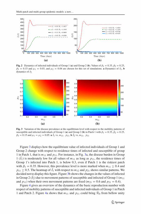
Fig. 2 Dynamics of infected individuals of Group 1 (a) and Group 2 (b). Values of β1 = 0.35, β2 = 0.25,β3 = 0.15 and μ1 = 0.03, and μ2 = 0.04 are chosen for this set of simulations. a Dynamics of I1, bdynamics of I2

0.1

0.2

0.3

0.4

0.5

0.6

0.7

0.8

0.9

1

50

100

150

200

250

300

350

400

450

0.2 0.4 0.6 0.8 1 0.2 0.4 0.6 0.8 10.1

0.2

0.3

0.4

0.5

0.6

0.7

0.8

0.9

1

50

100

150

200

250

(a) (b)

Fig. 3 Variation of the disease prevalence at the equilibrium level with respect to the mobility patterns ofsusceptible and infected individuals of Group 1 (a) and Group 2 (b) in Patch 1 with β1 = 0.35, β2 = 0.25,β3 = 0.15 and μ1 = μ2 = 0.05. a I1 vs. m11, p11, b I2 vs. m11, p11

Figure 3 displays how the equilibrium value of infected individuals of Group 1 andGroup 2 change with respect to residence times of infected and susceptible of group1 in Patch 1, that is m11 and p11. For instance, in Fig. 3a, the disease burden in Group1 ( I1) is moderately low for all values of m11 as long as p11, the residence times ofGroup 1’s infected into Patch 1, is below 0.3, even if Patch 1 is the riskiest patchwith β1 = 0.35. However, this prevalence level is more marked when m11 ≥ 0.4 andp11 ≥ 0.5. The heatmap of I1 with respect to m12 and p21 shows similar patterns. Wedecided not to display this figure. Figure 3b shows the changes in the values of infectedin Group 2 ( I2) due to movement patterns of susceptible and infected of Group 1 (m11and p11) when their own movement patterns are fixed (m21 = 0.6 and p21 = 0.4).

Figure 4 gives an overview of the dynamics of the basic reproduction number withrespect of mobility patterns of susceptible and infected individuals of Group 1 in Patch1 and Patch 2. Figure 4a shows that m11 and p11 could bring R0 from bellow unity

123


0.2 0.4 0.6 0.8 1

0.2

0.4

0.6

0.8

1

0.80.911.11.21.31.41.51.61.7

0.2 0.4 0.6 0.8 1

0.2

0.4

0.6

0.8

1

0.850.90.9511.051.11.151.21.251.3

(a) (b)

Fig. 4 Variation of R0 with respect to the mobility patterns of susceptible and infected individuals ofGroup 1 in Patch 1 (a) and Patch 2 (b). Values of β1 = 0.2, β2 = 0.1 and β3 = 0.08 are chosen for this setof simulations. aR0 vs. m11, p11, bR0 vs. m12, p12

0 0.2 0.4 0.6 0.8 10.6

0.7

0.8

0.9

1

1.1

1.2

1.3

1.4

0 0.2 0.4 0.6 0.8 10

0.5

1

1.5

2

2.5

(a) (b)

Fig. 5 Variability of R0 with respect to m11, m12 and p11, p12. If all other parameters are fixed, R0increases with respect to m11 and m12. a R0 vs. m11, b R0 vs. p11

to above unity. Particularly, if m11 ≥ 0.4, thenR0 > 1, which lead to the persistenceof the disease. Also, R0 is much higher when m11 ≥ 0.7 and p11 ≥ 0.2. Figure 4bshows how R0 varies when the movement of infected and susceptible of Group 1 inPatch 2 change.

In Fig. 5, we revisit the variability of the basic reproduction number with respect ofmobility patterns of susceptible and infected individuals of Group 1 (Fig. 4). However,we obtain a clear picture on how it changes. Indeed, Fig. 5a suggests thatR0 increaseswith respect to m11 and m12; and p11 and p12 (Fig. 5b). However,R0 increases muchfaster with respect to p11 than to m11. Moreover, Fig. 5b confirms also the result ofTheorem 3.1, which states that the basic reproduction number increases with respectof pi j , that is the movement patterns of infected individuals.

Figure 6 showcases that, for a fixed number of groups (3 in this case), the basicreproduction number increases as the number of patches increases, and that indepen-dently of the values of the risk of infection of the added patches. This figure, also

123


Fig. 6 Effects of patchiness onthe basic reproduction numberR0 with u = 3. This risk ofinfection chosen for these 4patches are: β1 = 0.25,β2 = 0.15, β3 = 0.1, β4 = 0.08

0 0.1 0.2 0.3 0.4 0.5 0.6 0.7 0.8 0.9 10

0.5

1

1.5

2

2.5

confirms our the theoretical result in Item 3 of Theorem 3. It also shows a linearmonotonicity of R0(u, v) with respect to P. Other values of βs than those of Fig. 6exhibit similar patterns.

5 Global stability of equilibria

The global stability of equilibria for the general Model (2) happens to be very chal-lenging. In fact, for models with such intricated nonlinearities, it is shown in Huanget al. (1992) that multiple endemic equilibria may exist. In this section, we explorethe global stability of equilibria for some particular cases of the general model.

5.1 Identical mobility and no disease induced mortality

In this subsection, we suppose that the host mobility to the patches is independent ofthe epidemiological status and that we neglect the disease induced mortality. In thiscase, the dynamics of the total population is given by

N = � − μ ◦ N

Hence, limt→∞ N = �μ

:= N. By using the theory of asymptotic systems (Castillo-Chavez and Thieme 1995; Vidyasagar 1980), System (2) is asymptotically equivalentto:

⎧⎪⎪⎨

⎪⎪⎩

S = � − diag(S)Mdiag(B)diag−1(MT N)MT I − diag(μ)S + diag(η)RE = diag(S)Mdiag(B)diag−1(MT N)MT I − diag(ν + μ)EI = diag(ν)E − diag(γ + μ)IR = diag(γ )I − diag(η + μ)R

(7)

Model (7) generalizes models considered in Bichara et al. (2015). Let us denoteREq

0 (u, v) the corresponding basic reproduction number of Model (7). Its expressionis

123


REq0 (u, v) = ρ(diag(S∗)Mdiag(B)diag−1(MTS∗)MT diag(ν)diag−1((μ + ν)

◦ (μ + γ )))

The following theorem gives the global stability of the disease free equilibrium.

Theorem 5.1 Whenever the host-patch mobility configuration MMT is irreducible,

the following statements hold:

1. IfREq0 (u, v) ≤ 1, the DFE is globally asymptotically stable (GAS).

2. IfREq0 (u, v) > 1, the DFE is unstable.

Proof Let (wE , wI ) a left eigenvector of Zdiag(ν)diag−1((μ + ν) ◦ (μ + γ )) corre-sponding to ρ(Zdiag(ν)diag−1((μ + ν) ◦ (μ + γ ))) where

Z = diag(S∗)Mdiag(B)diag−1(MTS∗)MT

Hence,

(wE , wI )Zdiag(ν)diag−1((μ + ν) ◦ (μ + γ )) = (wE , wI )ρ(Zdiag(ν)diag−1

((μ + ν) ◦ (μ + γ )))

= (wE , wI )ρ(−FV−1)

SinceMMT is irreducible, thematrix Zdiag(ν)diag−1((μ+ν)◦(μ+γ )) is irreducible.

This implies that (wE , wI ) � 0.We consider the Lyapunov function

V (E, I) = (wE , wI )

(diag−1(μ + ν) 0u,u

diag(ν)diag−1((μ + ν) ◦ (μ + γ )) diag−1(μ + γ )

) (EI

)

The derivative of V (E, I) along trajectories of (7) is

V (E, I) = (wE , wI )

(diag(μ + ν)−1 0u,u

diag(ν)diag−1((μ + ν) ◦ (μ + γ )) diag−1(μ + γ )

)(EI

)

= (wE , wI )

(−diag(μ + ν) diag(S)Mdiag(B)diag−1(MT N)MT

diag(ν) −diag(μ + γ )

) (EI

)

where wE = wEdiag−1(μ + ν) + wIdiag(ν)diag−1((μ + ν) ◦ (μ + γ )) and wI =wIdiag−1(μ + γ ), or equivalently (wE , wI ) = (wE , wI )(−V−1).

Since diag(S) ≤ diag(S∗) and S∗ = N, we obtain (denoting I the identity matrix),

V (E, I) ≤ (wE , wI )(F + V )

(EI

)

= (wE , wI )(−V−1F − I

) (EI

)

123


=(REq

0 (u, v) − 1)

(wE , wI )

(EI

)

≤ 0.

We consider first the case whenREq0 (u, v) < 1. Let E be an invariant set contained in

�, where V (E, I) = 0. This set is reduced to the origin of R2u (i.e., (E, I) = (0, 0)).This, combined to the invariance of E , leads to R = 0 and S = S∗. Hence, the onlyinvariant set contained in �, such that V (E, I) = 0, is reduced to the DFE. Hence,by LaSalle’s invariance principle (Bhatia and Szegö 1970; LaSalle and Lefschetz1961), the DFE is globally asymptotically stable on �. Since � is an attracting set,we conclude that the DFE is GAS on the positive orthant R4u+ .

When REq0 (u, v) = 1, we can show that

V (E, I) = (wE+wI diag(ν)diag(μ + γ+δ)−1)diag(μ + ν)−1 (diag(S)−diag(S∗))·Mdiag(B)diag−1(MT N)MT I≤ 0.

Therefore, as above, LaSalle’s invariance principle allows to conclude.The instability of the DFE when REq

0 (u, v) > 1 follows from Diekmann et al.(1990); van den Driessche and Watmough (2002).

The following theorem provides the uniqueness of the endemic equilibrium.

Theorem 5.2 IfREq0 (u, v) > 1, Model (7) has a unique endemic equilibrium.

The proof of this theorem is similar to that of Theorem 5.3 in the next subsection.

5.2 Effective population size dependent risk

So far, the risk associated with each patch is represented by the constant vector B.However, in some cases, it is more appropriate to assume that the risk of catching adisease depends on the size of the population or crowd, that is the effective populationsize in each patch. In this subsection, we suppose that the risk of infection in each patchj is linearly proportional to the effective population size, that is N eff

j = ∑uk=1(mi j Si +

ni j Ei + pi j Ii + qi j Ri ). Hence,

β j (Neffj ) = β j

u∑

k=1

(mkj Sk + nkj Ek + pkj Ik + qkj Rk)

Hence, the rate at which susceptible individuals are infected in Patch j is, therefore

β j (Neffj )

∑uk=1 pkj Ik∑u

k=1(mkj Sk + nkj Ek + pkj Ik + qkj Rk):= β j

u∑

k=1

pkj Ik

123


Therefore, in this settings, the dynamics of the population in different epidemiologicalclasses take the form:

⎧⎪⎪⎪⎪⎪⎪⎪⎪⎪⎨

⎪⎪⎪⎪⎪⎪⎪⎪⎪⎩

Si = �i −v∑

j=1

β jmi j Si

u∑

k=1

pkj Ik − μi Si + ηi Ri ,

Ei =v∑

j=1

β jmi j Si

u∑

k=1

pkj Ik − (νi + μi )Ei

Ii = νi Ei − (γi + μi + δi )IiRi = γi Ii − (ηi + μi )Ri

(8)

System (8) could be written in a compact form as follows:

⎧⎪⎪⎨

⎪⎪⎩

S = � − diag(S)Mdiag(B)PT I − diag(μ)S + diag(η)RE = diag(S)Mdiag(B)PT I − diag(ν + μ)EI = diag(ν)E − diag(γ + μ + δ)IR = diag(γ )I − diag(η + μ)R

(9)

Clearly, System (9) is a particular case of System (2) when the transmission termtakes a modified density-dependent form. Positivity and boundedness properties ofsolutions of System (2) hold for those of System (9). The basic reproduction numberof Model (9), denoted by RDD

0 (u, v) is:

RDD0 (u, v) = ρ(diag(S∗)Mdiag(B)PT diag(ν)diag−1((μ + ν) ◦ (μ + γ + δ)))

We explore the properties of steady state solutions. The following result gives theglobal stability of the DFE. Its proof is similar to that of Theorem 5.1.

Corollary 5.1 Whenever the host-patch mobility configuration MPT is irreducible,

the following statements hold:

1. IfRDD0 (u, v) ≤ 1, the DFE is globally asymptotically stable.

2. IfRDD0 (u, v) > 1, the DFE is unstable.

The proof of the existence and uniqueness of the endemic equilibrium (EE) forModel (9) is done in two steps, by carefully crafting a new auxiliary system whoseEE uniqueness is tied to that of Model (9).

Let

A = diag−1(η + μ) diag(γ ) diag−1(γ + μ + δ) diag(ν),

L = diag−1(γ + μ + δ) diag(ν)

and K = diag−1(μ)diag(ν + μ) − diag−1(μ) diag(η) A (10)

We have the following lemma,

123


Lemma 5.1 Model (9) has a unique endemic equilibrium if the function

g(y) = diag−1(ν + μ) diag(S∗ − Ky)Mdiag(B)PT Ly,

has a unique fixed point.

Proof Let (S, E, I, R) an equilibriumpoint of System (9)with I � 0. This equilibriumsatisfies the following system:

⎧⎪⎪⎨

⎪⎪⎩

0 = � − diag(S)Mdiag(B)PT I − diag(μ)S + diag(η)R0 = diag(S)Mdiag(B)PT I − diag(ν + μ)E0 = diag(ν)E − diag(γ + μ + δ)I0 = diag(γ )I − diag(η + μ)R

(11)

We can easily see that R = AE and I = LE, where A, L and K are as defined in (10).Thus, I � 0 implies that E � 0 and R � 0.Hence, System (11) could be written only in terms of S and E, that is:

{S = diag−1(μ)

(� − diag(S)Mdiag(B)PT LE + diag(η) AE

)

E = diag−1(ν + μ) diag(S)Mdiag(B)PT L E(12)

Let x = diag−1(μ)�− S and y = E. Since S ∈ �, it is clear that x ≥ 0 and y ≥ 0.Expressing the system (12) into new variables, we obtain:

{x = diag−1(μ) f (x, y) − diag−1(μ) diag(η) A y (13a)

y = diag−1(ν + μ) f (x, y) (13b)

where

f (x, y) = diag(S∗ − x)Mdiag(B)PT Ly

It follows from (13b) that f (x, y) = diag(ν + μ) y, and hence (13a) implies thatx = Ky where

K = diag−1(μ)diag(ν + μ) − diag−1(μ) diag(η) A

After some algebraic manipulations, it could be shown that K > 0. Combiningthe fact that x = Ky and (13b), it follows that (13), and subsequently (11), could bewritten in the single vectorial equation:

y = g(y)

where

g(y) = diag−1(ν + μ) f (Ky, y)

= diag−1(ν + μ) diag(S∗ − Ky)Mdiag(B)PT Ly (14)

123


Thus, Model (9) has a unique endemic equilibrium I � 0 if and only if g(y) has aunique fixed point y � 0. The desired result is achieved.

Next, we present another lemma whose proof is straightforward:

Lemma 5.2 The function g(y) has a fixed point y if and only if y is an equilibriumof y = F(y) where

F(y) = diag(ν + μ)g(y) − diag(ν + μ)y

The proof of this lemma is straightforward.

Theorem 5.3 Under the assumption that the host-patch mobility configurationMPT

is irreducible, Model (9) has a unique endemic equilibrium wheneverRDD0 (u, v) > 1.

Proof By using Lemma 5.1 and Lemma 5.2, the uniqueness of EE for Model (9) isequivalent to the uniqueness of an EE for this system

y = F(y) (15)

when RDD0 (u, v) > 1. Therefore, we will prove that the auxiliary system (15) has

an unique EE. In fact, we will prove that this equilibrium is globally attractive ifRDD

0 (u, v) > 1. The proof of the latter is based on Hirsch’s theorem (Hirsch 1984),by using elements of monotone systems. The Jacobian of the vector field F(y) is:

F ′(y) = diag(ν + μ) (g′(y) − I)

=(−diag

(Mdiag(B)PT Ly

)K + diag(S∗ − Ky)Mdiag(B)PT L

)

− diag(ν + μ) I

= − diag(ν + μ) I − diag(Mdiag(B)PT Ly

)K + diag(S∗ − Ky)M

diag(B)PT L .

where I is the identity matrix. Thematrix−diag(ν+μ) I−diag(Mdiag(B)PT Ly

)K

is a diagonal matrix and diag(S∗ −Ky)Mdiag(B)PT L is a nonnegative matrix (sinceS∗ − Ky = S). It follows that F ′(y) is Metzler and is irreducible since MP

T is.Therefore, System (15) is strongly monotone. Moreover, it is clear that the map F ′ :Ru −→ R

u × Ru is antimonotone. Also, F(0Ru ) = 0Ru and F ′(0Ru ) = g′(0Ru ) −

I = diag(S∗)Mdiag(B)PT L−I. Since ρ(g′(0Ru )) = ρ(diag(S∗)Mdiag(B)PT L) =RDD

0 (u, v) > 1,we deduce that F ′(0Ru ) has at least a positive eigenvalue and therefore0Ru is unstable. Therefore, System (15) has unique equilibrium y � 0Ru , which isglobally attractive, due toHirsch’s theorem (Hirsch 1984) (Theorem6.1).We concludethat Model (9) has a unique endemic equilibrium whenever RDD

0 (u, v) > 1. Note that with the choice of P = Mdiag−1(MT N) and δ = 0, System (9) is exactly

System (7). Therefore, their solutions have the same asymptotic behavior.

123


6 Conclusion and discussions

Heterogeneity in space and social groups are often studied separately and sometimesinterchangeably in the context of disease dynamics. Moreover, in these settings, sus-ceptibility of the infection is based on group or individual. In this paper, we proposea new framework that incorporates heterogeneity in space and in group for which thestructure of the latter is independent from that of the former. We define patch as a loca-tion where the infection takes place, which has a particular risk of infection. This riskis tied to environmental or hygienic or economic conditions that favors the infection.The likelihood of infection in each patch depends on both the risk of the patch andthe proportion of time each host spend in that environment. We argue that this patch-specific risk is easier to assess compared to the classical differential susceptibility orWAIFW matrices. Human host is structured in groups, where a group is defined as acollection of individuals with similar demographic, genetic or social characteristics.In this framework, the population of each patch at time t is captured by the temporalmobility patterns of all host groups visiting the patches, which in turn depends on thehost’s epidemiological status.

Under this framework, we propose a general SEIRS multi-patch and multi-groupmodel with differential state-host mobility patterns. We compute the basic reproduc-tion number of the system with u groups and v patches, R0(u, v), which depends onthe mobility matrices of susceptible, M, and infected, P. The disease persists whenR0 > 1 and dies out from all patches when R0(u, v) < 1 (Fig. 2), when MP

T isirreducible. When this matrix is not irreducible, the disease will persist or die out inall patches of the subsystem for which the configuration group-patch is irreducibleand will be decoupled from the remaining system.

We systematically investigate the effects of heterogeneity in mobility patterns,groups and patches on the basic reproduction and on disease prevalence. Indeed, wehave shown that, if the epidemiological parameters are fixed, the basic reproductionnumber is an increasing function of the entries of infected hosts’ movement matrix(e.g. Theorem 3.1). Also, if the number of groups is fixed, an increase in the numberof patches increases the basic reproduction number (e.g. see Theorem 3.2). Explicitexpressions of the basic reproduction numbers are obtained when the mobility matri-cesM and P are of rank one. That is, when, for all groups, susceptible (and infected)individuals’ residence times in all patches are proportional (Theorems 3.3 and 3.4). Itturns out that if the susceptible residence time matrix is of rank one and stochastic, thebasic reproduction number is independent ofM. Moreover, we also show that ifM isof rank one, its stochasticity is sufficient but not necessary for the basic reproductionnumber to be independent of M. However, if the infected residence time matrix P isof rank one, stochastic or otherwise, the basic reproduction number still depends onthe infected movement patterns.

The patch-specific risk vector B could also depend on the effective population size.We explored the case when this dependence is linear, that is when, for each patch j ,β j (N eff

j ) = β j∑u

k=1(mkj Sk +nkj Ek + pkj Ik +qkj Rk). In this case, the transmissionterm of our model is captured by a density dependent incidence. Moreover, we showthat this case is isomorphic to the general model, where the mobility patterns of hostdoes not dependent on the epidemiological class, that is when M = N = P = Q. We

123


prove that, in this case the disease free equilibrium is globally asymptotically stablewhenever R0 ≤ 1 while an unique endemic equilibrium exists ifR0 > 1.We suspect that the disease free equilibrium is globally asymptotically stablewheneverR0 ≤ 1 forModel (2), where the patch-specific risk is constant. A similar remark holdsfor the global stability of the endemic equilibrium of Model (9) and Model (2) whenR0 > 1. This is still under investigation. Further areas of extensions of this studyinclude more general forms of the patch-specific risks and when mobility patternsreflect the choices that individuals make at each point in time. These choices are basedon maximizing the discounted value of an economic criterion à la (Fenichel et al.2011; Perrings et al. 2014).

Acknowledgements We are grateful to two anonymous referees and the handling editor Dr. GabrielaGomes for valuable comments and suggestions that led to an improvement of this paper. We also thankBridget K. Druken for the careful reading and constructive comments. A. Iggidr acknowledges the partialsupport of Inria in the framework of the program STIC AmSud (project MOSTICAW).

References

Anderson RM, May RM (1991) Infectious diseases of humans. Dynamics and control. Oxford sciencepublications, Oxford

Arino J (2009) Disease in metapopulations model. In: Ma Z, Zhou Y, Wu J (eds) Modeling and dynamicsof infectious diseases. World Scientific Publishing, Singapore, pp 65–123

Arino J, Portet S (2015) Epidemiological implications of mobility between a large urban centre and smallersatellite cities. J Math Biol 71:1243–1265

Arino J, vandenDriesscheP (2006)Disease spread inmetapopulations. In: ZhaoX-O,ZouX (eds)Nonlineardynamics and evolution equations, vol 48. Fields Institute Communications, AMS, Providence, pp 1–13

Berman A, Plemmons RJ (1994) Nonnegative matrices in the mathematical sciences. SIAM, PhiladelphiaBhatia NP, Szegö GP (1970) Stability theory of dynamical systems. Springer, BerlinBichara D, Castillo-Chavez C (2016) Vector-borne diseases models with residence times—a Lagrangian

perspective. Math Biosci 281:128–138Bichara D, Kang Y, Castillo-Chavez C, Horan R, Perrings C (2015) Sis and sir epidemic models under

virtual dispersal. Bull Math Biol 77:2004–2034Bichara D, Holechek SA, Velázquez-Castro J, Murillo AL, Castillo-Chavez C (2016) On the dynamics of

dengue virus type 2 with residence times and vertical transmission. Lett Biomath 3:140–160Blythe SP, Castillo-Chavez C (1989) Like-with-like preference and sexual mixing models. Math Biosci

96:221–238Bonzi B, Fall A, Iggidr A, Sallet G (2011) Stability of differential susceptibility and infectivity epidemic

models. J Math Biol 62(1):39–64Castillo-Chavez C, Busenberg S (1991) A general solution of the problem of mixing of subpopulations

and its application to risk-and age-structured epidemic models for the spread of aids. Math Med Biol8:1–29

Castillo-Chavez C, Thieme HR (1995) Asymptotically autonomous epidemic models. In: Arino O, AxelrodDE, Kimmel M (eds) Mathematical population dynamics: analysis of heterogeneity, volume one:theory of epidemics. Wuerz, Winnipeg

Castillo-Chavez C, Bichara D, Morin BR (2016) Perspectives on the role of mobility, behavior, and timescales in the spread of diseases. Proc Natl Acad Sci 113:14582–14588

Cosner C, Beier J, Cantrell R, Impoinvil D, Kapitanski L, Potts M, Troyo A, Ruan S (2009) The effects ofhuman movement on the persistence of vector-borne diseases. J Theor Biol 258:550–560

DiekmannO,Heesterbeek JAP,Metz JAJ (1990)On the definition and the computation of the basic reproduc-tion ratio R0 in models for infectious diseases in heterogeneous populations. J Math Biol 28:365–382

Dushoff J, Levin S (1995) The effects of population heterogeneity on disease invasion.Math Biosci 128:25–40

123


Eckenrode S, Bakullari A, Metersky ML, Wang Y, Pandolfi MM, Galusha D, Jaser L, Eldridge N (2014)The association between age, sex, and hospital-acquired infection rates: results from the 2009–2011national medicare patient safety monitoring system. Infect Control Hosp Epidemiol 35:S3–S9

Falcón-Lezama JA,Martínez-VegaRA,Kuri-Morales PA, Ramos-Castañeda J, AdamsB (2016)Day-to-daypopulation movement and the management of dengue epidemics. Bull Math Biol 78:2011–2033

Fall A, Iggidr A, Sallet G, Tewa J-J (2007) Epidemiological models and lyapunov functions. Math ModelNat Phenom 2:62–68

Fenichel E, Castillo-Chavez C, CeddiaMG, Chowell G, Gonzalez Parra P, Hickling GJ, Holloway G, HoranR, Morin B, Perrings C, Springborn M, Valazquez L, Villalobos C (2011) Adaptive human behaviorin epidemiological models. PNAS 108:6306–6311

Hethcote HW, Thieme HR (1985) Stability of the endemic equilibrium in epidemic models with subpopu-lations. Math Biosci 75:205–227

Hirsch M (1984) The dynamical system approach to differential equations. Bull AMS 11:1–64Horn RA, Johnson CR (1985) Matrix analysis. Cambridge University Press, New YorkHuang W, Cooke K, Castillo-Chavez C (1992) Stability and bifurcation for a multiple-group model for the

dynamics of HIV/AIDS transmission. SIAM J Appl Math 52:835–854Iggidr A, Sallet G, Tsanou B (2012) Global stability analysis of a metapopulation sis epidemic model. Math

Popul Stud 19:115–129Iggidr A, Sallet G, Souza MO (2016) On the dynamics of a class of multi-group models for vector-borne

diseases. J Math Anal Appl 2:723–743Jacquez JA, SimonCP,Koopman J, Sattenspiel L, PerryT (1988)Modeling and analyzingHIV transmission:

the effect of contact patterns. Math Biosci 92:119–199Jacquez JA, Simon CP, Koopman J (1996) Core groups and the r0s for subgroups in heterogeneous SIS

and SI models. In: Mollison D (ed) Epidemics models: their structure and relation to data. CambridgeUniversity Press, Cambridge, pp 279–301

Kaplan V, Angus DC, Griffin MF, Clermont G, Scott Watson R, Linde-zwirble WT (2002) Hospitalizedcommunity-acquired pneumonia in the elderly: age-and sex-related patterns of care and outcome inthe united states. Am J Respir Crit Care Med 165:766–772

Kermack W, McKendrick A (1927) A contribution to the mathematical theory of epidemics. Proc R SocA115:700–721

Lajmanovich A, Yorke J (1976) A deterministic model for gonorrhea in a nonhomogeneous population.Math Biosci 28:221–236

LaSalle JP, Lefschetz S (1961) Stability by Liapunov’s direct method. Academic Press, CambridgeMetz JA, Diekmann O (2014) The dynamics of physiologically structured populations, vol 68. Springer,

BerlinNold A (1980) Heterogeneity in disease-transmission modeling. Math Biosci 52:227Perrings C, Castillo-Chavez C, Chowell G, Daszak P, Fenichel EP, Finnoff D, Horan RD, Kilpatrick AM,

Kinzig AP, Kuminoff NV, Levin S, Morin B, Smith KF, SpringbornM (2014) Merging economics andepidemiology to improve the prediction and management of infectious disease. Ecohealth 11:464–475

Prothero RM (1977) Disease and mobility: a neglected factor in epidemiology. Int J Epidemiol 6:259–267Rodríguez DJ, Torres-Sorando L (2001) Models of infectious diseases in spatially heterogeneous environ-

ments. Bull Math Biol 63:547–571Ruktanonchai NW, SmithDL, De Leenheer P (2016) Parasite sources and sinks in a patched ross-macdonald

malariamodelwith human andmosquitomovement: implications for control.MathBiosci 279:90–101Rushton S, Mautner A (1955) The deterministic model of a simple epidemic for more than one community.

Biometrika 42:126–132Salmani M, van den Driessche P (2006) A model for disease transmission in a patchy environment. DCDS

Ser B 6:185–202Sattenspiel L, Dietz K (1995) A structured epidemic model incorporating geographic mobility among

regions. Math Biosci 128:71–91Sattenspiel L, Simon CP (1988) The spread and persistence of infectious diseases in structured populations.

Math Biosci 90:341–366. Nonlinearity in biology and medicine (Los Alamos, NM, 1987)van den Driessche P, Watmough J (2002) reproduction numbers and sub-threshold endemic equilibria for

compartmental models of disease transmission. Math Biosci 180:29–48Vidyasagar M (1980) Decomposition techniques for large-scale systems with nonadditive interactions:

stability and stabilizability. IEEE Trans Autom Control 25:773–779

123


Xiao Y, Zou X (2014) Transmission dynamics for vector-borne diseases in a patchy environment. J MathBiol 69:113–146

Yorke JA, Hethcote HW,NoldA (1978) Dynamics and control of the transmission of gonorrhea. Sex TransmDis 5:51–56

123

Multi-patch and multi-group epidemic models: a new...

Documents

Transcript of Multi-patch and multi-group epidemic models: a new...