Zienkiewicz, A. K., Barton, D. A. W., Porfiri, M., & Di Bernardo, M. (2015).Data-driven stochastic modelling of zebrafish locomotion. Journal ofMathematical Biology, 71(5), 1081-1105. https://doi.org/10.1007/s00285-014-0843-2

Publisher's PDF, also known as Version of record

License (if available):CC BY

Link to published version (if available):10.1007/s00285-014-0843-2

Link to publication record in Explore Bristol ResearchPDF-document

The final Open Access publication is available at Springer via http://dx.doi.org/10.1007/s00285-014-0843-2

University of Bristol - Explore Bristol ResearchGeneral rights

This document is made available in accordance with publisher policies. Please cite only the publishedversion using the reference above. Full terms of use are available:http://www.bristol.ac.uk/pure/about/ebr-terms

J. Math. Biol.DOI 10.1007/s00285-014-0843-2 Mathematical Biology

Data-driven stochastic modelling of zebrafishlocomotion

Adam Zienkiewicz · David A. W. Barton · Maurizio Porfiri ·Mario di Bernardo

Received: 9 May 2014 / Revised: 26 August 2014© The Author(s) 2014. This article is published with open access at Springerlink.com

Abstract In this work, we develop a data-driven modelling framework to reproducethe locomotion of fish in a confined environment. Specifically, we highlight the primarycharacteristics of the motion of individual zebrafish (Danio rerio), and study how thesecan be suitably encapsulated within a mathematical framework utilising a limited num-ber of calibrated model parameters. Using data captured from individual zebrafish viaautomated visual tracking, we develop a model using stochastic differential equationsand describe fish as a self propelled particle moving in a plane. Based on recent exper-imental evidence of the importance of speed regulation in social behaviour, we extendstochastic models of fish locomotion by introducing experimentally-derived processesdescribing dynamic speed regulation. Salient metrics are defined which are then usedto calibrate key parameters of coupled stochastic differential equations, describing

Electronic supplementary material The online version of this article (doi:10.1007/s00285-014-0843-2)contains supplementary material, which is available to authorized users.

This work was supported by the Engineering and Physical Sciences Research Council (EPSRC) underGrant number EP/I013717/1, and the National Science Foundation (USA) under Grant numbersCMMI-0745753 and CMMI-1129820. DAWB was supported by EPSRC under Grant numberEP/K032739/1.

A. Zienkiewicz · D.A.W. Barton ·M. di Bernardo (B)Department of Engineering Mathematics, University of Bristol, Bristol, UKe-mail: m.dibernardo@bristol.ac.uk

M. di BernardoDepartment of Electrical Engineering and ICT, University of Naples Federico II, Naples, Italy

M. PorfiriDepartment of Mechanical and Aerospace Engineering, New York University Polytechnic Schoolof Engineering, New York , USAe-mail: mporfiri@nyu.edu

123

A. Zienkiewicz et al.

both speed and angular speed of swimming fish. The effects of external constraintsare also included, based on experimentally observed responses. Understanding thespontaneous dynamics of zebrafish using a bottom-up, purely data-driven approach isexpected to yield a modelling framework for quantitative investigation of individualbehaviour in the presence of various external constraints or biological assays.

Keywords Fish locomotion · Computational biology · Stochastic models ·Zebrafish · Ornstein–Uhlenbeck

Mathematics Subject Classification 37N25 · 46N60 · 97M60 · 60H10 · 91B70 ·37B70

1 Introduction

The coordinated motion of groups of animals, and in particular of fish shoals, hasbeen widely studied both from experimental and theoretical perspectives (Partridge1982; Huth and Wissel 1992; Camazine et al. 2001; Couzin et al. 2002; Krause andRuxton 2002; Buhl et al. 2006; Kolpas et al. 2007; Pillot et al. 2011; Moussaïd etal. 2011; Gautrais et al. 2012; Vicsek and Zafeiris 2012). Numerous authors haveproposed a wide variety of theoretical models, for example the canonical Vicsek-typemodels (Vicsek et al. 1995) along with those by Czirók et al. (1997, 1999) whichdescribe mobile agents as identical self-propelled particles with heading directionsupdated via the integration of noisy local-neighbourhood interaction rules. More elab-orate models of collective motion have also been proposed which may account forrepulsive and attractive forces between fish (or other animals), for example those byAoki (1982), Reynolds (1987), Huth and Wissel (1992), Couzin et al. (2002), Grégoireand Chaté (2004), Chaté et al. (2008), Kolpas et al. (2013). Within all of these models,the dynamics of the group behaviour are dissected into individual rules from whichcomplex coordinated motions emerge. It is critical therefore to establish predictiveand tractable models for the behavioural response of isolated individuals, upon whichto study and construct models of sociality.

The degree to which individual behaviour modulates group dynamics, and cor-respondingly, how interactions with conspecifics affects individual response, can betested with a modelling cycle driven by precise experimental data. The recent workof Gautrais et al. serves as an important example of this process. Specifically, a data-driven model of spontaneous fish movement was first derived by Gautrais et al. (2009).Then, using a bottom-up methodology, a model of group motion from data gatheredat the level of the individual was developed by Gautrais et al. (2012). Unlike manyother models of collective motion, this approach enables all model parameters to beestimated directly from experimental data. Based on evidence that the fish considered(Kulia Mugil) are best described in terms of their turning speed and its autocorrelation,Gautrais et al. have developed a model referred to as a ‘Persistent Turning Walker’(PTW). This model is based on an Ornstein–Uhlenbeck (O-U) stochastic differentialequation (SDE) governing the turning speed of an agent with a fixed forward speed.In addition, the effects of environmental confinement were considered, providing a

123

Data-driven stochastic modelling of zebrafish locomotion

versatile methodology for incorporating fixed boundaries, obstacles and other fish,within the same model framework.

Recent experimental studies, including those by Krause and Ward (2005), Herbert-Read and Perna (2011), Katz et al. (2011), Berdahl et al. (2013), Herbert-Read et al.(2013), show that the speed response of fish play an important role in fish interaction.For example, a comprehensive study by Katz et al. (2011) reveals the subtle modulationof turning and speeding responses of groups of golden shiners in relation to their con-specifics. Important conclusions from this work include the observation that speedregulation may be a dominant component of interaction, where subsequent alignmentbetween neighbouring fish emerges from the interplay between attraction and repul-sion. With respect to this latter conclusion, some models including that of Strömbom(2011), have demonstrated the characteristic hallmarks of collective motion with a richdiversity of dynamics such as swarming, and circular and directed milling, emergingsolely from inertial local attraction between individuals. The study by Katz et al. alsoexamined the importance of higher order interactions, namely a non-trivial 3-bodycomponent which may contradict the pervasive assumption of models which exclu-sively integrate pairwise interactions. Supporting experimental work by Herbert-Readand Perna (2011) also suggested the absence of an empirically justifiable alignmentrule for schooling mosquitofish, suggesting that group polarisation is an emergentproperty. In this study, speed regulation was again found to be a key reaction mech-anism due to group interactions, especially repulsion from close neighbours, withclearly defined zones of interaction.

Most commonly, models of schooling consider fish as agents with fixed forwardspeed (Couzin et al. 2002; Gautrais et al. 2009, 2012), and thus prevent us fromexploring the role of speed regulation in collective dynamics. Existing models ofcollective motion which do consider variable speed agents (Reynolds 1987; Huth andWissel 1994; Toner and Tu 1998; D‘Orsogna et al. 2006; Strefler et al. 2008; Ebelingand Schimansky-Geier 2008; Abaid and Porfiri 2010; Strömbom 2011; Mishra et al.2012) either describe self-propelled particles as a continuum dynamical system, orrather consider the effects of noise on the absolute velocity. Thus far however, noneof these approaches have been fully validated against experimental data in terms oftheir description of speed modulation.

The primary aim of this paper is to extend the approach by Gautrais et al. (2009)to develop a data-driven modelling framework describing the individual locomotionof zebrafish. Selected here primarily for their strong propensity to form social groups(Miller and Gerlai 2008; Saverino and Gerlai 2008; Miller and Gerlai 2012), labo-ratory studies with zebrafish also benefit from their short intergenerational time andcomparatively high reproductive rate. Yielding extensive genomic homologues withboth humans and rodents, zebrafish have emerged as one of the predominant speciesfor neurobiological, developmental and behavioural studies (Gerlai 2003; Kuo andEliasmith 2005; Miklósi and Andrew 2006; Lawrence 2007; Kalueff et al. 2014). Inthis work, we find that modelling zebrafish motion requires an additional, experimen-tally calibrated process governing the variation of swimming speed. In light of recentstudies such as those by Katz et al. (2011), Herbert-Read and Perna (2011), Berdahl etal. (2013), indicating that speed regulation is a key response of similar fish to externalstimuli, this latter modification represents a shift away from many canonical models,

123

A. Zienkiewicz et al.

which prescribe a constant speed, and provides the foundations for a novel modellingapproach for studying zebrafish social behaviour.

The modelling process addressed in this work employs a bottom-up approach,using data analysed from experimentally observed zebrafish trajectories, primarilyin terms of position/velocity time-series data, to inform an empirical model of indi-vidual swimming locomotion. Based on the direct analysis of experimental zebrafishtrajectory data obtained via automated computer vision techniques at the DynamicalSystems Laboratory (New York University Polytechnic School of Engineering, NY,USA), we clarify whether the stochastic PTW models of spontaneous fish motion,developed by Gautrais et al. (2009), can be applied to suitably describe the locomo-tion of zebrafish. We wish to emphasise that the modelling framework presented inthis paper can provide the foundation for future extensions which capture group leveldynamics of zebrafish shoals and their interaction with semi-autonomous artificialstimuli (Aureli et al. 2012; Kopman et al. 2012; Aureli et al. 2010; Aureli and Porfiri2010).

2 Materials and methods

2.1 Ethics statement

The experimental data for this analysis was provided by the Dynamic Systems Labo-ratory, New York University Polytechnic School of Engineering, NY, USA. Trajectorydata for isolated fish analysed in this study are derived from source data publishedin the recent work of Butail et al. (2014) (‘No Robot’ control condition). All exper-iments were conducted following the protocols AWOC-2012-101 and AWOC-2013-103 approved by the Animal Welfare Oversight Committee of the New York UniversityPolytechnic School of Engineering.

2.2 Animals and environment

Wild-type zebrafish (Danio rerio) were used in all experiments, acquired from anonline aquarium (LiveAquaria.com, Rhinelander, Wisconsin, USA). Subjects age wasbetween 6 to 8 months, inferred from their average body length (BL) of approximately3 cm. Fish were kept in 37.8 l (10 US gallon) holding tanks with a maximum of 20individuals in each. A photoperiod of 12 h light / 12 h dark was sustained prior toexperimentation as per Cahill (2002). Water temperature in the holding tanks wasmaintained at 27±1 ◦C with a pH of 7.2. Fish were fed daily at 7 pm with commercialflake food (Hagen Corp./Nutrafin Max, USA). Experiments were started after a 10 daysacclimatization period.

2.3 Apparatus

The setup and apparatus for this study is described by Butail et al. (2014). Experimen-tal subjects were monitored in a 120× 120× 20 cm tank, supported on an aluminium

123

Data-driven stochastic modelling of zebrafish locomotion

Fig. 1 Schematic of experimental apparatus for observing, tracking and analysing free-swimming zebrafish.Fish are transferred to experimental tank (120 × 120 × 20 cm) with water level of 10 cm, lit by overheadfluorescent tubes and shielded by dark curtains. Overhead digital video-camera records motion of individualzebrafish, with real-time object tracking at 5 Hz achieved using a desktop computer running MATLAB.Video frames and trajectory data are stored for subsequent analysis

frame, with a water depth of 10 cm (see Fig.1). The side length of the tank was thusapproximately equal to 40 BL. The surface of the tank was covered with a white contactpaper to enhance the contrast for automated tracking. Video recording was accom-plished using a Microsoft LifeCam (USB interfaced) camera mounted 150 cm abovethe water surface, providing a single overhead video feed at a resolution of 640× 480pixels at 5 fps. At this resolution, the location of a fish was represented by approxi-mately 20–50 pixels of each frame. Illumination was provided by diffused overheadlighting from four 25 W fluorescent tubes (All-Glass Aquarium, preheat aquariumlamp, UK). Video image analysis and real-time multi-target tracking was achievedusing software developed in MATLAB (R2011a, Mathworks), sampled at 5 Hz on a2.5 GHz dual-core Intel desktop computer with 3 Gb RAM (detailed description oftracking presented by Butail et al. (2013).

Experimental data consisted of individual video frames and trajectories consistingof two-dimensional position xt = [x, y]t , with the origin at the centre of the tank, usinga Cartesian coordinate system, and instantaneous velocity vt = [x, y]t computedusing a Kalman filter such that the mean square error is continuously minimised.A full description of the Kalman filter and the associated measurement model usedfor velocity estimation can be found in the supplementary material of Butail et al.(2013). Fish were thus tracked as point masses, with heading information reconstructedfrom the velocity vectors. We expect analogous results to be obtained via the methodfor heading reconstruction presented in Gautrais et al. (2009). Future work will beperformed using full shape tracking technique described in Bartolini et al. (2014) toassess the accuracy of different approaches for heading estimation from velocity data.

2.4 Experimental procedure

A total of ten experimental observations were used for this investigation, each track-ing the free-swimming trajectories of a different, experimentally naive, individualrandomly selected from the population. Fish were removed from the holding tank

123

A. Zienkiewicz et al.

using a small hand net and released into the experimental tank. Each observation waspreceded with ten minutes of habituation time allowing the fish to swim freely andacclimatise to the novel environment of the experimental tank, as reported by Wonget al. (2010). The motion of each fish was recorded for 5 min (300 s), sampled at 5 Hzproducing 1,500 position and velocity data samples per individual. Automated track-ing was performed on video frame data in real-time, with minor adjustments madeafter each observation to repair missing trajectory points.

2.5 Data extraction and pre-processing

Data for each observation was stored both as a sequence of image frames and a uniquecomma-separated data file containing the frame number and 2-dimensional positionxt and velocity data vt . The instantaneous speed ut at time t was calculated from thevector norm of the velocity, with ut = ‖vt‖. The turning speed at a given time stepωt is approximated using the (signed) angle turned between consecutive time stepst → t +Δt , to calculate a forward (angle) difference as follows:

ωt = sgn[vt+Δt × vt

]z

1

Δtcos−1

(vt+Δt · vt

‖vt+Δt‖‖vt‖)

(1)

where [·]z denotes the z-component of the cross product whose sign provides theturning direction (anti-clockwise positive). The time step Δt = 1/ fs is the reciprocalof the sampling frequency ( fs = 5 Hz). Note that this definition of ωt is consistentwith that in Gautrais et al. (2009), and associates fish turning speed with the rate ofchange of the orientation of the velocity vector.

The model described in this paper is designed to study swimming zebrafish, asopposed to additional locomotory patterns, such as freezing or thrashing near obstacles(boundaries) as defined by Bass and Gerlai (2008). To obtain suitable data representingswimming behaviour, we used a simplified version of a method described by Kopmanet al. (2012), pre-processing the ten raw observation data sets (denoted F1 . . . F10) toextract data segments (60 s) of equal duration in the following way:

1. Raw (speed) data was initially smoothed with a moving average window of 3 sam-ples, then segmented such that contiguous segments are isolated when fish is mov-ing with a speed above the threshold umin = 1 BL s−1. The original (unsmoothed)data is subsequently used for the steps that follow.

2. If the duration between consecutive segments was less than a time threshold τs =2 s, the two segments were joined so that fish were regarded as not swimming onlyif the duration of the speed dropping below threshold, umin, exceeded τs .

3. Resulting data segments were subdivided into intervals of equal length τl represent-ing a continuous time-series of swimming data from an individual fish. Segmentsshorter than τl were discarded such that we obtain continues data segments ofequal duration.

The isolated swimming data segments are denoted S1 . . . Sn and provide the dataused for subsequent model development. Subsequent parameter estimation was carried

123

Data-driven stochastic modelling of zebrafish locomotion

on individual segments with average parameter sets calculated for each individual fish[F1 . . . F10] based on the swimming data isolated for each observation.

2.6 Numerical implementation

Although an exact solution to the generalised O-U equation we will use in (7) exists,given by Gillespie (1996), nonlinearities in our model hamper its use. In order tocalculate discretised solutions to the model SDEs in (8), expressed in the formdXt = a(Xt )dt + b(Xt )dWt , we therefore employed the Euler-Maruyama method,approximating the true solution X with a Markov chain M where

Mt+Δt = Mt + α(Mt )Δt + β(Mt )ΔWt (2)

Here, Δt is the time step duration and ΔWt are i.i.d. normal random variables withmean equal to zero and variance Δt (Kloeden and Platen 1992).

Simulated trajectories in this work were realised by iterating a random walker (RW)path in the plane, using numerically computed values of speed Ut and turning speedΩt over the interval t = 0→ T in time steps of duration Δt . At each iteration t , thecurrent heading direction φt was updated according to the value of Ωt and the walkermoved forwards by a distance UtΔt . Specifically, heading directions were calculatedas follows:

φt = ((φt−Δt + π +ΩtΔt) mod 2π)− π (3)

where shifts by π and modulo operator ensure the heading angle varies smoothlyin [−π, π ]. The position xt was subsequently updated at each time-step using

xt = [x, y]t = [x, y]t−Δt + [cos φt , sin φt ] UtΔt (4)

and the corresponding velocity vt , computed by the backwards difference formula

vt = (xt − xt−Δt ) /Δt (5)

For all simulations, the initial positions of random walkers x0 were randomly distrib-uted within the simulation arena with uniformly distributed heading angles [−π, π ]and initial speed and turning speed U0 = μu , Ω0 = 0. The simulation time-step wasset equal to the experimental sample rate such that Δt = 0.2 s.

Following the calculation of both fW and fc at a given time step t (discussed in §4),the updated values of Ut and Ωt were found using the method in (2), with values of Ωt

restricted in the range ±15 rad s−1 in accordance to the observed maximum angularspeed.

3 Experiments

The swimming speeds u of 10 individuals were found to range from extended stationaryperiods, up to maximum speeds of approximately 31 cm s−1, corresponding to just over

123

A. Zienkiewicz et al.

−60

0

60F 1

F 2F 3

F 4F 5

−60

060

−60

0

60F 6

−60

060

F 7

−60

060

F 8

−60

060

F 9

−60

060

F 10

y (cm)

x (c

m)

Fig

.2R

awtr

ajec

tory

data

capt

ured

from

10ze

brafi

sh(v

eloc

itypl

ots)

.Obs

erva

tions

wer

em

ade

for

5m

inpe

rin

divi

dual

fish,

swim

min

gin

ash

allo

w,s

quar

eta

nk(1

20×

120×

20cm

,10

cmw

ater

dept

h).A

utom

ated

visu

altr

acki

ngre

cord

edth

epl

anar

posi

tion

ofth

efis

hx t

with

inth

eta

nkat

5H

z,ca

lcul

atin

gsa

mpl

eve

loci

tyv t

usin

ga

Kal

man

filte

r.T

hehe

adin

gdi

rect

ion

and

mag

nitu

deof

velo

city

are

indi

cate

dby

colo

ured

arro

ws,

incr

easi

ngfr

ombl

ueto

red.

Swim

min

gda

taw

asex

trac

ted

from

allfi

shap

artf

rom

F4

and

F8

whi

chw

ere

foun

dto

swim

erra

tical

lyw

ithlo

ngpe

riod

sof

free

zing

123

Data-driven stochastic modelling of zebrafish locomotion

10 body lengths (BL) per second (1 BL ≈ 3 cm). The average speed across the entirepopulation was 3.53 BL.s−1 with a standard deviation of 2.48 BL s−1. Fish trajectories,shown in Fig. 2, were found to vary between individuals: some performed erratic,tightly winding manoeuvres (e.g. F4); whilst others had more fluid trajectories whichexplored an increased area of the tank (e.g. F1, F3, F5). We also found strong, persistentwall-following behaviour (thigmotaxis) (e.g. F6, F7, F10) along with extended periodsof freezing or thrashing behaviour (e.g. F2, F8, F9).

3.1 Swimming trajectory analysis

Using the data segmentation process described earlier, we isolated 28 segments ofswimming data, each 1 min in duration, representing 8 out of the 10 raw observations,where F4 and F8 failed to produce data which met all filtering criteria for swimming.The pre-processing method was also found to eliminate periods of excessive thrashing,characterised by large amplitude fluctuations in ωt . Speed and turning speed time seriesdata ut for each segment, labelled consecutively from S1 to S28, are shown in-situ withthe corresponding raw data in supplementary Figs. S1 and S2.

Analysis of the 28 min of data, isolated for active swimming behaviour for 8 fish,yielded a (increased) combined mean swimming speed of 4.65 BL s−1 with (reduced)standard deviation of 2.01 BL s−1; in good agreement with other studies e.g. Fuimanand Webb (1988), Plaut (2000) which report the mean speed of zebrafish groupsto be ∼ 13 cm.s−1(4.3 BL s−1). Mean turning speed was found to be −0.02 rad s−1

with a standard deviation of 1.30 rad s−1, indicating negligible turning direction pref-erence, with the convention that positive turning speeds represent turns to the left,negative to the right. Maximum and minimum values of turning speed were foundto be −14.73 and 14.28 rad s−1 respectively, suggesting a (global) absolute maxi-mum turning speed max(|ω|) ≈ 15 rad s−1. Maximum turning speeds were foundto be close to the upper limit detectable between consecutive samples at frequencyfs , where ωmax = π fs = 5π ≈ 15.71 rad s−1. Such high speed turns however areobserved with very low frequency across filtered swimming segment data, with turnsfaster than 5 rad s−1 accounting for less than 1% of all samples. Isolated swimmingtrajectory portraits (Fig. 3) display the variety of different characteristic behavioursdescribed earlier. In particular, we observed strong wall-following behaviour whichleads to an individual bias of the turning speed in the direction of rotation around thewalls.

During active phases of swimming, the instantaneous speed ut of an individualwas found to have a well-defined mean, yet highly variable with rapid bursts of for-ward thrust corresponding to the natural tail-beat frequency between 0.5 and 2 Hz,identified through spectrographic analysis of the time series data. Additionally, weobserved strong correlations between the time onset of bursts in turning speed withthose in instantaneous speed (Fig. 4a, b). Strong correlations were also found betweenthe magnitude of ut and the variance of ωt (Fig. 4c). This characteristic feature maybe associated with momentum conservation from tail-beating, which simultaneouslyprovides both axial force and torque, to produce forward and turning motion, respec-tively (Sfakiotakis et al. 1999).

123

A. Zienkiewicz et al.

Fig

.3Is

olat

edsw

imm

ing

segm

entt

raje

ctor

ies.

Den

oted

S 1..

.S 2

8,e

ach

traj

ecto

ry,o

f60

sin

dura

tion,

are

colo

ured

acco

rdin

gto

the

orig

inat

ing

fish

obse

rvat

ion

(F1..

.F

10),

whe

requ

alif

ying

data

has

been

extr

acte

dfr

om8

outo

f10

uniq

uein

divi

dual

s(F

4,

F8

faile

dto

prov

ide

suffi

cien

tdat

a)

123

Data-driven stochastic modelling of zebrafish locomotion

0 10 20 30 40 50 600

5

10u

(BL.

s−1 )

0 10 20 30 40 50 60−15

0

15

Time (s)

ω (

rad.

s−1 )

0 2 4 6 8−15

0

15

ω (

rad.

s−1 )

u (BL.s−1)

a

b

c

Fig. 4 Example data from swimming segment S9. a and b Time series data for speed ut and turning speed ωtrespectively, with associated relative frequency histograms and fitted normal distribution p.d.f (smooth red,blue curves). Vertical delineations in time-series plots indicate minima in ut with a prescribed minimumseparation of 0.5 s (2 Hz). Identical lines in ωt time-series highlight a temporal correlation where speedminima are generally associated with peaks in |ωt | (thin blue trace). c Values of ωt against ut indicating acorrelation with increased probability of large turning speed ωt values as ut decreases

The distribution of instantaneous speed ut was found to be approximately normalwith a natural truncation at u = 0 cm s−1. Individually parameterised Gaussian densityfunctions therefore yield a good approximation to the distributions of ut (Fig. 4a).Analysis of ωt (Fig. 4b) similarly indicated that a normal probability density functionprovides reasonable approximations to experimental data, with a mean close to zero.In general however, the distributions of ωt were found to be more sharply peaked thana Gaussian, with heavy tails due to a low proportion of extreme values of turning, bothleft (ω � 0) and right (ω � 0), resulting in larger estimates of the standard deviationand flattening of the corresponding Gaussian probability distribution function (pdf).As such, a normal distribution is found to be appropriate when the sample standarddeviation σω < 1.5 rad s−1. Above this value, a normal distribution fails to capture boththe sharp peak around the mean, and the finite probability of rapid changes in heading.In the model we describe later in this section, the speed process ut is assumed to be astationary Gaussian process, whilst the turning speed ωt is assumed to be a Gaussianprocess with varying variance. Additionally, these processes are coupled such that werecover both the observed cross-correlation and a correction to the distribution of theturning speed.

Autocorrelation functions (ACF) for both ut and ωt were computed for all segments,revealing consistent and well-defined properties. Both processes display a large pos-itive correlation at short time-lags which decays with an approximately exponentialenvelope with varying degrees of noisy oscillation. We quantified the decay rate of theACF by considering the lag-one autocorrelation coefficient r1 of discretely sampledsignal {Xk}Nk=1, given by

r1 =∑N−1

k=1 (Xk − X)(Xk+1 − X)∑N

k=1(Xk − X)2(6)

where X is the sample mean.We considered the associated correlation time τ for the ACFs, where τ =

−Δt/ln(r1) was used to parameterise an exponential function ACFest = exp(−t/τ)

123

A. Zienkiewicz et al.

0 5 10−0.5

0

0.5

1

Lag time (s)

AC

F

ut

0 1 2 3 4 5−0.5

0

0.5

1

Lag time (s)

ωt

ba

Fig. 5 Autocorrelation of S9 speed and turning speed. a ACFu up to 5 s of lag with exponential approxima-tion (black dashes) ACFu ≈ exp (−t/τu), τu = 3.54 s (b) ACFω up to 5 s of lag with ACFω ≈ exp (−t/τω),τω = 0.29 s. Autocorrelation half-life for either process is thus approximated by τ ln(2), where τ is theone-step autocorrelation coefficient

estimating the autocorrelation decay envelope. Across the majority of segments, aexponential approximation provides a good estimate for both ACFu and ACFω (exam-ple shown for segment S9 in Fig. 5). The average autocorrelation half-life (τ ln 2) for ut

and ωt across segments, were found to be approximately 1.37 and 0.28 s, respectively.

4 Modelling

Our analysis of zebrafish trajectory data suggests that a model in which speed isheld constant may be insufficient to describe the individual and collective motion ofzebrafish and other similar species of small, schooling fish. Compared with the smooth,continuous motion of larger fish, for example Kulia mugil (BL ≈ 20 cm) modelledby Gautrais et al. (2009), the variance in swimming speed for smaller zebrafish (BL≈ 3 cm) is large. Many factors influence the range and fluctuations of swimming speed,with drag being the primary physical component, scaling with the square of the wettedsurface area. In the presence of viscous drag, with a flow regime dependent on thespecific Reynolds number, different aquatic species have evolved a range of swimmingstyles as described by Sfakiotakis et al. (1999). Specifically for zebrafish, their smallsize and tail morphology results in a burst-and-coast mode of locomotion, which hasbeen found to be more efficient than a continuous swimming style, as discussed byWeihs (1972), Muller et al. (2000).

The key features of both signals considered independently, instantaneous speed ut

and turning speed ωt , are well approximated by stationary, Gaussian processes withexponentially decaying autocorrelation functions. These observations lead us to adoptthe formalism of a continuous-time autoregressive system with two independentlyparameterised Gaussian processes for ut and ωt . The basis of our model is thus anextension of the PTW model presented by Gautrais et al. (2009) in which the turningspeed Ωt of a simulated random walker is modelled by a signal St , a stochastic processof the Ornstein–Uhlenbeck (O-U) family with the general form

dSt = θ(μ− St )dt + σdWt (7)

with equilibrium (relaxation) value μ, rate of mean-reversion θ , and variance σ ofthe standard Wiener process Wt . As t → ∞ the stationary solution of this SDE

123

Data-driven stochastic modelling of zebrafish locomotion

has a Gaussian distribution with a mean and variance approaching μ and σ 2/2θ ,respectively (Gardiner 2009).

In our extended model, we consider two coupled stochastic equations, describingboth the speed Ut and turning speed Ωt as follows:

dUt = θu(μu −Ut )dt + σudWt (8a)

dΩt = θω(μω + fW −Ωt )dt + fcdZt (8b)

where the SDEs for speed (8a) and turning speed (8b) have the same general form pre-sented earlier in (7), describing random processes exhibiting noisy relaxation to a meanμ and, importantly, with an exponentially decaying ACF with rate θ = 1/τ . Additivenoise is driven by the Wiener processes dW and dZ , with variances parameterised byσ 2

u and f 2c , acting on the differentials of position and heading respectively.

In order to recover the observed correlation between the magnitude of ut and vari-ance of ωt (e.g. Fig 4c), we introduce the function fc = fc(Ut , σω, σ0, μu), whichcouples the two processes such that the variance of the random fluctuations of turningspeed Ωt depends on the speed Ut . Wall (boundary) avoidance is achieved by incor-porating a second function fW = fW (φW , dW ) in (8b), which models the tendencyof fish to avoid collisions with the tank walls, where dW and φW are the distance andangle of projected collision with a boundary, given the velocity at a given time step.The features encapsulated by these two additional functions fW and fc, including theestimation of all model parameters, are described in what follows.

4.1 Selection of wall avoidance function fW

Following the approach of Gautrais et al. 2009, the term fW is constructed to reflect theobserved turning speed distribution as a function of distance dW (Gautrais et al. 2009),or time tW (Gautrais et al. 2012) with which a projected collision with the boundarywould occur given the current position and velocity of the fish. To quantify this effect,we calculate the distribution of a ‘wall-corrected’ value of the turning speed ωc whichis positive when the direction of a turn is away from the collision boundary and viceversa, such that

ωct ={|Ωt | if sgn(Ωt ) = sgn(φWt )

−|Ωt | otherwise(9)

The direction of the induced turn characterised by fW is therefore prescribed bycalculating the (signed) angle φW between the current heading and the normal at thepoint of collision. The plots in Figs. S3 and S4 display show ωc calculated from eachsegment, as a function of dW and tW respectively.

Based on the fact that the turning dependence was very similar for both dW and tW ,we choose the form

fW (φW , dW ) = sgn(φW )A exp(BdW ) (10)

123

A. Zienkiewicz et al.

Retaining the formalism of the general O-U process (7), fW provides a smooth,exponentially increasing bias to the equilibrium value of the Ω turning speed process,in the direction which increases the projected distance (or time) to collision. ParametersA and B control the strength and decay of the repulsion fW and are estimated fromexperimental data as described in the following section (Parameter estimation). Asimilar analysis on the effect of wall boundaries on speed regulation suggested thatspeed is only marginally influenced by the wall distance (Fig. S5, S6). For this reasonwe opted not to include a functional dependence on either dW or tW for the speedprocess in (8a) as we have for turning speed.

As the repulsive turning effect supplied by fW does not implicitly prevent trajec-tories from crossing the simulated boundaries, we also include an additional hard-boundary condition. Our simple strategy is to model wall encountering events as fullyinelastic collisions, such that the speed Ut of a random walker passing through aboundary at time t is set to zero, leaving its position unchanged from the previoustime step, so that xt ← xt−Δt .

In order to replicate experimental conditions, simulated trajectories were mod-elled in a bounded, rectangular arena. However, a finite, rectangular simulation arenapresents discontinuous boundaries at each corner which must be smoothed to preventcompeting repulsion by perpendicular walls near the vertices from creating singulari-ties for point-like random walkers. By rounding the edges of the simulation arena withquarter-circles of radius Rc, we avoid unrealistic turning behaviour at the corners ofthe tank, where a value of Rc = 10 cm was found to sufficiently reduce undesirableartefacts in these regions.

4.2 Selection of coupling function fc

The joint distribution of experimental data on ut and ωt was found to be highlyasymmetric, with a much larger proportion of faster turns occurring at low speeds. Acomposite log-density plot of cross-correlated data is shown in Fig. 6a.

Fast turning speeds are associated with lower forward speeds due to mechanics offish locomotion. To model this relationship we therefore require a coupling betweenthe two SDEs in (8a) and (8b), such that we obtain similar distributions of speed Ut

and turning speed Ωt to those observed in the experiments. Specifically, we substitutethe variance parameter σ in the general O-U process description in (7) with a functionfc in the form of an exponential decay with respect to the speed Ut . Due to heavy-tailsof the observed turning speed distribution, calibration using a maximum likelihoodestimation (MLE) following the method described by van den Berg (2011) (assuminga standard O-U process with a normal distribution) will tend to overestimate σ fromsource data ωt and overly increase the variability of the simulated turning speed processΩt . We account for this by choosing fc such that

1. When Ut approaches zero, the function returns the upper bound, say σ0 on thevariance of the turning speed (to be estimated from the experimental observations),or equivalently

limUt→0

fc = σ0, σ0 > σω (11)

2. The function approaches zero as Ut goes to infinity.

123

Data-driven stochastic modelling of zebrafish locomotion

[experiment]

u (cm.s−1)

ω (

rad.

s−1 )

0 5 10 15 20 25 30−10

−5

0

5

10[simulated]

U (cm.s−1)

Ω (

rad.

s−1 )

0 5 10 15 20 25 30

log(

rel

.freq

. )

−9

−8

−7

−6

−5

a b

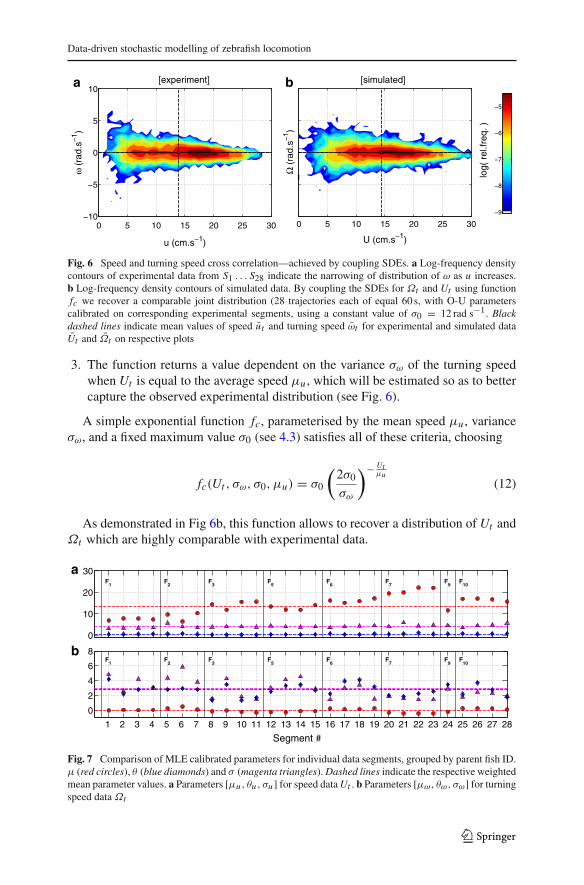
Fig. 6 Speed and turning speed cross correlation—achieved by coupling SDEs. a Log-frequency densitycontours of experimental data from S1 . . . S28 indicate the narrowing of distribution of ω as u increases.b Log-frequency density contours of simulated data. By coupling the SDEs for Ωt and Ut using functionfc we recover a comparable joint distribution (28 trajectories each of equal 60 s, with O-U parameterscalibrated on corresponding experimental segments, using a constant value of σ0 = 12 rad s−1. Blackdashed lines indicate mean values of speed ut and turning speed ωt for experimental and simulated dataUt and Ωt on respective plots

3. The function returns a value dependent on the variance σω of the turning speedwhen Ut is equal to the average speed μu , which will be estimated so as to bettercapture the observed experimental distribution (see Fig. 6).

A simple exponential function fc, parameterised by the mean speed μu , varianceσω, and a fixed maximum value σ0 (see 4.3) satisfies all of these criteria, choosing

fc(Ut , σω, σ0, μu) = σ0

(2σ0

σω

)− Utμu

(12)

As demonstrated in Fig 6b, this function allows to recover a distribution of Ut andΩt which are highly comparable with experimental data.

0

10

20

30F

1F

2F

3F

5F

6F

7F

9F

10

1 2 3 4 5 6 7 8 9 10 11 12 13 14 15 16 17 18 19 20 21 22 23 24 25 26 27 28

0

2

4

6

8F

1F

2F

3F

5F

6F

7F

9F

10

Segment #

b

a

Fig. 7 Comparison of MLE calibrated parameters for individual data segments, grouped by parent fish ID.μ (red circles), θ (blue diamonds) and σ (magenta triangles). Dashed lines indicate the respective weightedmean parameter values. a Parameters [μu , θu , σu ] for speed data Ut . b Parameters [μω, θω, σω] for turningspeed data Ωt

123

A. Zienkiewicz et al.

4.3 Parameter estimation

The six parameters [μ, θ, σ ]u,ω for individual segments S1 . . . S28 were found usingMLE, following the method of van den Berg (2011), under the assumption that sourcedata ut and ωt both come from independent Gaussian processes described by (7).Equivalent parameters corresponding to the individual fish F1, F2, F3, F5, F6, F7, F9,F10 were subsequently calculated by averaging over the corresponding segments val-ues extracted from each fish. The relationship between segments to parent observationdata and MLE calibrated parameter values are shown in Fig. 7, indicating generallyconsistent parameters across individuals. We also calculated a global set of mean para-meters [μu, θu, σu] (speed) and [μω, θω, σω] (turning speed), computed by weightingthe individual means by the number of segments isolated for each fish, e.g.

μu =∑10

i=1 niμu[Fi ]∑10

i=1 ni(13)

where ni is the number of segments isolated for each fish Fi . The values calculatedin this way are found below, and also in Table 1 alongside parameter values for eachindividual fish. They are:

μu = 14.02 cm s−1(4.67 BL s−1)

θu = 4.21 s−1

σu = 0.59 cm s−1

μω = −0.02 rad s−1

θω = 2.74 s−1

σω = 2.85 rad s−1 (14)

The parameters A and B of the wall repulsion function fW in (10), specifying thestrength and range respectively, were found by calculating the distance dW which afish, at a given sample position, is projected to collide with the tank wall, given its cur-rent velocity. For each data sample, we constructed the wall-corrected turning speedωc as described in (9) by modifying the sign of ωt to reflect turning either towards oraway from the boundary. By plotting sample values of ωc against the projected dis-tance dW , or time tW to wall collision, we observe a distinct bias for turns which favourimpact avoidance (ωc > 0) as dW decreases. To approximate this bias, we used a non-parametric locally weighted least squares (LOESS) model (Gijbels and Prosdocimi2010), fitting the resulting interpolation with a parametric exponential function. Usingthis method, averaging across swimming segments, we estimated the parameters A andB in (10) determining the repulsive (turning) effect of the boundary on turning speed asa function of dW . An example of the two-step interpolation for segment S27 is shown inFig. 8a. By considering only segments with which a reasonable fit could be obtained[S2, S3, S4, S6−11, S13, S16, S17, S19, S20, S22, S23, S25−28], we found average para-meter values A = 2.25± 0.70 rad s−1 and B = −0.11± 0.04 cm. For completeness,

123

Data-driven stochastic modelling of zebrafish locomotion

Tabl

e1

Mea

npa

ram

eter

valu

esfo

rea

chfis

hF

1..

.F

10,c

alcu

late

dfr

om28

isol

ated

data

segm

ents

.

F1

F2

F3

F4

F5

F6

F7

F8

F9

F10

#of

segm

ents

43

40

44

40

14

(28)

u(t

)μ

u7.

555

8.89

914

.406

N/A

12.8

4116

.135

20.9

64N

/A11

.719

16.6

4214

.02

θ u0.

592

0.66

10.

298

N/A

0.42

60.

633

0.77

1N

/A0.

717

0.74

10.

59

σu

3.35

04.

447

3.98

1N

/A4.

086

4.11

84.

810

N/A

4.65

14.

689

4.21

ω(t

)μ

ω0.

028

0.28

0−0

.183

N/A

−0.1

870.

206

−0.3

84N

/A−0

.221

0.22

1-0

.02

θ ω3.

077

2.85

81.

971

N/A

2.99

63.

347

2.17

5N

/A3.

456

2.60

62.

74

σω

3.65

14.

676

2.30

4N

/A3.

649

2.35

51.

599

N/A

2.91

42.

128

2.85

Wei

ghte

dav

erag

espr

ovid

ing

aco

mm

on(g

loba

l)se

tof

para

met

ers

are

indi

cate

din

bold

123

A. Zienkiewicz et al.

0 10 20 30−5

0

5

dw

(cm)

ωc (

rad.

s−1 )

1.66exp(−0.12dw)

0 1 2 3−5

0

5

tw

(s)

ωc (

rad.

s−1 )

3.09exp(−3.04tw)

b

a

Fig. 8 Effect of boundary on turning speed with respect to the projected distance and time to collision withtank wall on segment S27 data. Non-parametric (LOESS) regression (black dashed lines) highlight increasedturning to avoid collisions (ωc > 0). a Wall corrected turning speed ωc is plotted as a function of theprojected distance dW to impact with a wall. Exponential function ωc = Ad eBd dW (red curve) approximatesa ‘soft’ repulsion as a function of projected distance with fitted parameters Ad = 2.14 rad s−1,Bd =−0.16 cm. b wall-corrected turning speed ωc is plotted as a function of the projected time tW to impactwith a wall. Exponential function ωc = At eBt tW (red curve) approximates repulsion as a function ofprojected distance with fitted parameters At = 3.00 rad s−1, Bt = −2.98 s

we also calculated parameters values for A and B for a time-to-collision dependencetW (see Fig. 8b), averaging over segments [S4, S7, S8−11, S13, S16, S18−28] to giveA = 2.25 ± 0.62 rad s−1 and B = −1.68 ± 0.53 s. From our analysis we found nocompelling evidence supporting a stronger functional dependence of turning speed oneither dW or tW thus we proceeded with a wall-avoidance function dependent solelyon projected collision distance dW and the collision angle φW . Graphical depictionsof the dependence of ωc and ut on projected collision distance dW and time tW for allsegment data can be found in supplementary Figs. S3–S6.

Heuristically, we found that a magnified value of A was required to produce turn-ing behaviour comparable to experimental observations. After many realisations ofrandom walkers with various calibrations, we chose to increase the above value ofA by a factor of 3 such that we simulate all random walkers with A = 6.75 rad s−1

and B = −0.11 cm, calculating fW (dW , φW ) from Eq. (10). This discrepancy resultseither from interpolating fW with an insufficient number of data points close to theboundaries, or the compensation required to account for oversimplification of the wallavoidance model.

Finally, we estimated the saturation parameter σ0 in (12) so as to obtain a similarcorrelation between simulated values of Ut and Ωt , with consideration given to therange and distribution of observed turning speeds. Although the absolute maximumvalue was found to be≈ 15 rad s−1, the distribution of experimental ωt is heavy-tailed

123

Data-driven stochastic modelling of zebrafish locomotion

Table 2 Global simulation parameters

Parameter description Symbol Unit Value

Simulation time step Δt s 0.2

Simulated tank (square) side length L cm 120

Rounded edge circle radius rc cm 10

Maximum turning speed variance σ0 rad s−1 12

Max. turning speed (cut-off) n/a rad s−1 15

Wall avoidance function amplitude A rad s−1 6.75

Wall avoidance function decay B cm –0.11

such that values of |ω| > 10 rad s−1 account for less than 0.2% of recorded samples.We therefore prescribed a reasonable upper bound to the function fc by finding σ0such that the probability of generating turning speed values Ωt from (8b) below aspeed of approximately 10 rad s−1, is within the 2-sigma (∼ 95%) confidence intervali.e. 2σ ≈ 10 rad s−1, where σ is the long term variance of the output process. Thevariance σ 2 of Ωt was estimated by assuming a general O-U process where, for thesaturation variance σ0 we have σ 2 = σ 2

0 /2θω (Gardiner 2009). Using the maximumωt as an estimate of two standard deviations (2σ ), we obtain the formula

σ0 = max(ωt )√

2θω

2(15)

Using the values max(ωt ) = 10 rad s−1 and θω = 2.81 s−1, the global average valuefrom (14), we obtain the maximum variance parameter value σ0 ≈ 12 rad s−1. Accord-ingly, the resulting composite distribution of simulated values of Ut and Ωt for allsegment calibrations, shown in Fig. 6b, indicates a good approximation to the experi-mental distribution in Fig. 6a.

4.4 Model consistency

Initial validation of the model was conducted by comparing the trajectories, and under-lying metrics, of individual swimming segments to those of simulated random walk-ers with SDE parameters calibrated from the corresponding experimental segments.The remaining parameters were fixed globally across all segments using the valuesdescribed earlier in this section, summarised in Table 2. A square simulation arena withside length L = 120 cm was also defined to match the dimensions of the experimentaltank.

Data simulated across a range of sample generation frequencies, 1000–5 Hz (Δt =0.001–0.2 s) using identical stochastic processes dWt and d Zt , indicated that trajecto-ries and their underlying statistics (distributions, ACFs etc.) were sufficiently robustto increasing values of Δt over three orders of magnitude (see Fig. S7). Using a valueΔt = 0.2 s was therefore found to provide a good compromise between numerical

123

A. Zienkiewicz et al.

Fig. 9 Comparison between simulated random walker for S17 and experimental segment data. Data high-lights the key metrics to compare swimming segment S17 (blue) against those of a random walker (red),with parameters calibrated directly on the experimental segment. a Time series and distribution for speeddata Ut . b Time series and distribution for turning speed data Ωt . c Cross-correlation between Ut and Ωt .d Autocorrelation function ACFu . e Autocorrelation function ACFω . f Trajectory vector comparison

accuracy and computational efficiency1, with a corresponding sample generation rateof 5 Hz matching that of the experimental acquisition frequency.

An example simulation, calibrated on segment S17, is shown in Fig. 9, comparedwith the experimental data for both speed and turning speed. Simulated speed data(shown in red) yields a normal distribution which corresponded well with the experi-mental data (Fig. 9a). The speed autocorrelation function ACFu (Fig. 9d) was also ingood agreement with that of the experimental source data, in particular capturing theinitial decay prior to the zero crossing. Simulated turning speed data (blue), generatedby a modified (coupled) O-U type process, was found to have a distribution which ismore sharply peaked than a Gaussian process, and in good agreement with source dataΩt (Fig. 9b). Here, we note an additional effect of the SDE coupling, where fc restrictsthe probability of high speed turning to periods of reduced forward speed. A directresult of this is to produce a turning speed distribution with a sharper peak aroundthe mean (μω ≈ 0), and with heavier tails such that extreme values of Ω are foundwith low probability, but more often than would be produced by a normally distributed(unmodified) O-U process. The joint distribution of speed and turning speed (Fig. 9c)also presents a successful recovery of the experimental distribution, characterised bya narrowing of the turning speed distribution as speed increases. By appropriatelycoupling the SDEs via fc we therefore achieve both recovery of the cross-correlationbetween ut and ωt , and a favourable modification to the distribution of ωt to matchthose observed experimentally. Similarly, for the corresponding autocorrelation ACFω

(Fig. 9e), we are able to capture the characteristic exponential decay, with a rate verysimilar to the experimentally observed value. A final comparison is made in Fig. 9f,showing the resulting 60 s RW trajectory portrait and velocity vector plot, overlaid onthe experimental source data.

To support the inclusion of the coupling function fc in our proposed model, wesimulated comparable trajectories in the absence of coupling (fixed σω). Simulated

1 Random walk trajectories with a duration of 60 s are computed in approximately 0.2 s in the currentimplementation with Δt = 0.2 s

123

Data-driven stochastic modelling of zebrafish locomotion

−60

0

60 F1

F2

F3

F5

−60 0 60−60

0

60 F6

−60 0 60

F7

−60 0 60

F9

−60 0 60

F10y

(cm

)

x (cm)

Fig. 10 Comparing experimental and simulated trajectories of individual swimming zebrafish. Uniqueparameters sets are found for each fish (F1, F2, F3, F5, F6, F7, F9, F10) by averaging values calibratedfor associated swimming segments. Experimentally observed swimming trajectories of zebrafish (blue) areplotted as composites of (disjoint) segment data. Simulated trajectories (red) are calculated and plottedfor an equal duration to the underlying experimental data. O-U parameters for each fish can be found inTable 1 (trajectories for F4 and F8 not calculated due to lack of suitable swimming data). All random walkertrajectories were computed with the global simulation parameters given in Table 2

realisations for representative experimental segments S3 and S17 are shown in Fig. S14,both with and without the coupling between Ut and turning speed variance σω. In theuncoupled trials, we clearly fail to capture a reasonable estimate for the joint distribu-tion of speed and turning speed (see column B in Fig. S14). Without fc to restrict theturning speed variance at high speeds, we find a more normal spread of Ωt which failsto capture the sharp peaks of the experimental distributions (column D). The one-waycoupling between two processes should have no effect on the distribution and auto-correlation of speed data (columns B and E), however we also note that we do notfind significant effects on the turning speed ACF (column F). Importantly, we find thattrajectories produced by the coupled model appear to be qualitatively more consistentwith experimental segment trajectories (column A). We note a higher propensity toenter longer lasting/long path length spiralling when the process are uncoupled, fea-tures which are reduced by the coupling as large turning speed variance (increasedrange in either direction) is reduced at high speeds—and therefore only available tothe random walker at lower speeds where less distance will be covered during such aturn. We also note that decoupling the processes reduces the propensity to elicit wall-following behaviour when calibrated on segments exhibiting these phenomena (againdue to the increase range of turning speeds when decoupled or conversely because,when coupled, the turning speed distribution is more sharply peaked around zero).

Plots for all segments (coupled model), comparing a single random walker real-isation to experimental source data, can be found in the supplementary information(Figs. S8–S13). We also refer again to plots depicting the dependence of speed andwall-corrected turning speed on projected distance and time to boundary collision insupplementary Figs. S3–S6.

123

A. Zienkiewicz et al.

x (cm)

y (c

m)

a

−60 0 60−60

0

60

x (cm)

b

−60 0 60−60

0

60

x (cm)

c

−60 0 60−60

0

60 % time

0

0.2

0.4

Fig. 11 Trajectory density comparison between experimental and simulated data. Trajectory data in theform of density plots, with pixel color representing the percentage time spent at each location (1,680 s at5 Hz for each comparison). a Composite of experimental segment data. b Composite of 8, individuallycalibrated random walkers from Fig. 10. c Single random walker realisation, calibrated with weightedaverage parameter values found in (14)

Further tests of model consistency are provided by comparing eight random walkertrajectories, simulated using the averaged parameter values for individual fish F1, F2,F3, F5, F6, F7, F9 and F10 found in Table 1, to composite zebrafish trajectories fromthe corresponding experimental segments S1 . . . S28. Single random walker realisa-tions, calibrated for each fish are shown in Fig. 10, simulated for a time T = 60ns

where ns is the number of segments isolated for each fish. We observe that broadlysimilar qualitative turning characteristics of each zebrafish are recovered, includingthe propensity for wall-following behaviour. From these simulations, we find thatthe model is able to effectively extract and reproduce trajectory data which closelyapproximates the swimming motion, and subtleties of individual fish, and also howthe underlying statistics may be used to predict a form of ‘passive’ thigmotactic-likebehaviour2. Specifically, the approximate ratio σω/θω is found to provide a good pre-dictor of the observed thigmotactic-like behaviour that is well captured by the model.In order of increasing ratio, fish F6, F7 and F10 exhibit the most consistent wall-following behaviour, with values of σω/θω < 1. Consequently, fish which are foundto spend a larger fraction of time away from the walls, for example F2, F5, F1, in orderof decreasing ratio, are found to have σω/θω > 1.

Our final observation was a comparison between the trajectories of the eight indi-vidually calibrated random walks described above, to the trajectory of a single ran-dom walker, parameterised with the weighted-average values given in (14). Theplots in Fig. 11a–c) indicate, respectively, the relative density of positions in thetank/simulation area for experimental swimming trajectories, composite density ofthe eight individually calibrated random walkers, and the trajectory density of a sin-gle random walker simulated with the parameter set defined in (14), computed foran equivalent duration (28 × 60 = 1,680 s). Trajectories in Fig. 11a indicate a clearpreference of zebrafish to swim in close proximity to the tank walls with minimaldepartures into the centre of the tank. In comparison, the density plot for the individu-

2 We denote ‘passive’ thigmotactic-like behaviour as occurrences of wall-following which is not driven byexplicit modelling of psychological effects, for example in seeking protections from predators

123

Data-driven stochastic modelling of zebrafish locomotion

ally calibrated simulations (Fig. 11b) indicated increased variation in the area exploredby random walkers, with more activity in the central region. By performing a weightedaverage across all available swimming data (Fig. 11c), specifying a set of appropriatemean-model parameters, we found that a single (1,680 s duration) realisation of themodel reproduced a comparable density structure to that of the composite individuals,with significant wall-following behaviour and only a slightly increased frequency ofdepartures toward the centre.

5 Conclusions

A model of spontaneous zebrafish motion has been presented which captures theapproximate distribution of speed and angular speed of swimming fish, accountingfor both the autocorrelation and interdependence of these processes. Analysis of sim-ulated trajectories suggests that our model describes many of the salient features ofzebrafish locomotion, including the emergence of a thigmotactic-like (wall-following)behaviour when model parameters are calibrated on fish exhibiting similar patterns ofmotion. Specifically we find that this ‘passive’ wall-following behaviour results froma model in which only repulsion from the wall is present. The novel feature of thismodel, extending the ‘Persistent Turning Walker’ model due to Gautrais et al., is tocapture the intrinsic speed variation of zebrafish and other small fish.

Importantly, by allowing speed to vary in our model, further progress can be madein the development of group models which can address the most recent experimentalfindings for similar fish species. We refer specifically to the findings of Katz et al.(2011) and Herbert-Read and Perna (2011), which report that speed regulation is theprimary response governing the interaction between conspecifics and their environ-ment.

Further development of these models, informed directly from experimental data,represents a significant departure from some canonical approaches where fish are mod-elled with constant speed and conspecific interactions result in changes only to theirheading direction, or angular speed. Direct calibration of the model to experimentallyobserved fish trajectories results in a purely data-driven model and provides the neces-sary foundations for the future objective of understanding modelling the dynamics ofmulti-fish shoals. The results of the model are encouraging and provide a solid basisfor future investigations into fish social response.

Acknowledgments We also gratefully acknowledge the contributions of Fabrizio Ladu and Sachit Butailat the Dynamical Systems Laboratory, New York University Polytechnic School of Engineering, for pro-viding experimental data and visual tracking software used in our analysis. MdB would like to thank theDynamical Systems Laboratory for hosting him during the preparation of this manuscript and to acknowl-edge support from the Network of Excellence MASTRI Material e Strutture Intelligenti (POR CampaniaFSE 2007/2013).

Open Access This article is distributed under the terms of the Creative Commons Attribution Licensewhich permits any use, distribution, and reproduction in any medium, provided the original author(s) andthe source are credited.

123

A. Zienkiewicz et al.

References

Abaid N, Porfiri M (2010) Fish in a ring: spatio-temporal pattern formation in one-dimensional animalgroups. J R Soc Interface 7(51):1441–1453

Aoki I (1982) A simulation study on the schooling mechansim in fish. B Jpn Soc Sci Fish 48(8):1081–1088Aureli M, Fiorilli F, Porfiri M (2012) Portraits of self-organization in fish schools interacting with robots.

Phys D 241(9):908–920Aureli M, Kopman V, Porfiri M (2010) Free-locomotion of underwater vehicles actuated by ionic polymer

metal composites. IEEE/ASME Trans Mech 15(4):603–614Aureli M, Porfiri M (2010) Coordination of self-propelled particles through external leadership. EPL

92(4):40,004Bartolini T, Butail S, Porfiri M (2014) Temperature influences sociality and activity of freshwater fish.

Environ Biol Fish. doi:10.1007/s10641-014-0318-8Bass SLS, Gerlai R (2008) Zebrafish (Danio rerio) responds differentially to stimulus fish: the effects of

sympatric and allopatric predators and harmless fish. Behav Brain Res 186(1):107–117Berdahl A, Torney CJ, Ioannou CC, Faria JJ, Couzin ID (2013) Emergent sensing of complex environments

by mobile animal groups. Science 339(6119):574–576Buhl J, Sumpter DJT, Couzin ID, Hale JJ, Despland E, Miller ER, Simpson SJ (2006) From disorder to

order in marching locusts. Science 312(5778):1402–1406Butail S, Bartolini T, Porfiri M (2013) Collective response of zebrafish shoals to a free-swimming robotic

fish. PLoS One 8(10):e76, 123Butail S, Polverino G, Phamduy P, Del Sette D, Porfiri M (2014) Influence of robotic shoal size, con-

figuration, and activity on zebrafish behavior in a free-swimming environment. Behav Brain Res275:269–280

Cahill GM (2002) Clock mechanisms in zebrafish. Cell Tissue Res 309(1):27–34Camazine S, Deneubourg JL, Franks NR, Sneyd J, Theraulaz G, Bonabeau E (2001) Self-organisation in

biological systems. Princeton University Press, USAChaté H, Ginelli F, Grégoire G, Peruani F, Raynaud F (2008) Modeling collective motion: variations on the

Vicsek model. Eur Phys J B 64(3–4):451–456Couzin I, Krause J, James R (2002) Collective memory and spatial sorting in animal groups. J Theor Biol

218(1):1–11Czirók A, Stanley H, Vicsek T (1997) Spontaneously ordered motion of self-propelled particles. J Phys A

30(5):1375–1385Czirók A, Vicsek M, Vicsek T (1999) Collective motion of organisms in three dimensions. Phys A 264(1–

2):299–304D‘Orsogna M, Chuang Y, Bertozzi A, Chayes L (2006) Self-propelled particles with soft-core interactions:

patterns, stability, and collapse. Phys Rev Lett 96(10):104, 302Ebeling W, Schimansky-Geier L (2008) Swarm dynamics, attractors and bifurcations of active Brownian

motion. Eur Phys J Spec Top 157(1):17–31Fuiman L, Webb P (1988) Ontogeny of routine swimming activity and performance in zebra danios

(Teleostei: Cyprinidae). Anim Behav 36(1):250–261Gardiner C (2009) Stochastic methods. Springer, BerlinGautrais J, Ginelli F, Fournier R, Blanco S, Soria M, Chaté H, Theraulaz G (2012) Deciphering interactions

in moving animal groups. PLoS Comput Biol 8(9):e1002, 678Gautrais J, Jost C, Soria M, Campo A, Motsch S, Fournier R, Blanco S, Theraulaz G (2009) Analyzing fish

movement as a persistent turning walker. J Math Biol 58(3):429–445Gerlai R (2003) Zebra fish: an uncharted behavior genetic model. Behav Genet 33(5):461–468Gijbels I, Prosdocimi I (2010) Loess. Wiley Interdisciplin Rev Comput Stat 2(5):590–599. doi:10.1002/

wics.104Gillespie D (1996) Exact numerical simulation of the Ornstein–Uhlenbeck process and its integral. Phys

Rev E 54(2):2084–2091Grégoire G, Chaté H (2004) Onset of collective and cohesive motion. Phys Rev Lett 92(2):025, 702Herbert-Read JE, Krause S, Morrell LJ, Schaerf TM, Krause J, Ward AJW (2013) The role of individuality

in collective group movement. Proc R Soc B 280(1752):20122, 564Herbert-Read JE, Perna A (2011) Inferring the rules of interaction of shoaling fish. PNAS 108(46):18,

726–18, 731Huth A, Wissel C (1992) The simulation of the movement of fish schools. J Theor Biol 156(3):365–385

123

Data-driven stochastic modelling of zebrafish locomotion

Huth A, Wissel C (1994) The simulation of fish schools in comparison with experimental data. Ecol Model76:135–146

Kalueff AV, Stewart AM, Gerlai R (2014) Zebrafish as an emerging model for studying complex braindisorders. Trends Pharmacol Sci 35(2):63–75

Katz Y, Tunstrom K, Ioannou C, Huepe C, Couzin ID (2011) Inferring the structure and dynamics ofinteractions in schooling fish. PNAS 108(46):18, 720–18, 725

Kloeden P, Platen E (1992) Numerical solution of stochastic differential equations. Springer, BerlinKolpas A, Busch M, Li H, Couzin ID, Petzold L, Moehlis J (2013) How the spatial position of individuals

affects their influence on swarms: a numerical comparison of two popular swarm dynamics models.PLoS One 8(3):e58, 525

Kolpas A, Moehlis J, Kevrekidis IG (2007) Coarse-grained analysis of stochasticity-induced switchingbetween collective motion states. PNAS 104(14):5931–5935

Kopman V, Laut J, Polverino G, Porfiri M (2012) Closed-loop control of zebrafish response using a bioin-spired robotic-fish in a preference test. J R Soc Interface 10(78):20120, 540

Krause J, Ruxton G (2002) Living in Groups. Oxford University Press, UKKrause J, Ward A (2005) The influence of differential swimming speeds on composition of multi-species

fish shoals. J Fish Biol 67:866–872Kuo PD, Eliasmith C (2005) Integrating behavioral and neural data in a model of zebrafish network inter-

action. Biol Cybern 93(3):178–187Lawrence C (2007) The husbandry of zebrafish (Danio rerio): a review. Aquaculture 269(1–4):1–20Miklósi A, Andrew RJ (2006) The zebrafish as a model for behavioral studies. Zebrafish 3(2):227–234Miller N, Gerlai R (2012) From schooling to shoaling: patterns of collective motion in zebrafish (Danio

rerio). PLoS One 7(11):e48–e865Miller NY, Gerlai R (2008) Oscillations in shoal cohesion in zebrafish (Danio rerio). Behav Brain Res

193(1):148–151Mishra S, Tunstrom KR, Couzin ID, Huepe C (2012) Collective dynamics of self-propelled particles with

variable speed. Phys Rev E 86(1):011, 901Moussaïd M, Helbing D, Theraulaz G (2011) How simple rules determine pedestrian behavior and crowd

disasters. PNAS 108(17):6884–6888Muller U, Stamhuis E, Videler J (2000) Hydrodynamics of unsteady fish swimming and the effects of body

size: comparing the flow fields of fish larvae and adults. J Exp Biol 203:193–206Partridge B (1982) The structure and function of fish schools. Sci Am 246(6):114–123Pillot MH, Gautrais J, Arrufat P, Couzin ID, Bon R, Deneubourg JL (2011) Scalable rules for coherent

group motion in a gregarious vertebrate. PLoS One 6(1):e14, 487Plaut I (2000) Effects of fin size on swimming performance, swimming behaviour and routine activity of

zebrafish Danio rerio. J Exp Biol 203:813–820Reynolds CW (1987) Flocks, herds and schools: a distributed behavioural model. Comput Graph (ACM)

21(4):25–34Saverino C, Gerlai R (2008) The social zebrafish: behavioral responses to conspecific, heterospecific, and

computer animated fish. Behav Brain Res 191(1):77–87Sfakiotakis M, Lane D, Davies J (1999) Review of fish swimming modes for aquatic locomotion. IEEE J

Ocean Eng 24(2):237–252Strefler J, Erdmann U, Schimansky-Geier L (2008) Swarming in three dimensions. Phys Rev E 78(3):031,

927Strömbom D (2011) Collective motion from local attraction. J Theor Biol 283(1):145–151Toner J, Tu Y (1998) Flocks, herds, and schools: a quantitative theory of flocking. Phys Rev E 58(4):4828–

4858Vicsek T, Czirók A, Ben-Jacob E, Cohen I, Shochet O (1995) Novel type of phase transition in a system of

self-driven particles. Phys Rev Lett 75(6):4–7van den Berg T (2011) Calibrating the Ornstein–Uhlenbeck (Vasicek) modelVicsek T, Zafeiris A (2012) Collective motion. Phys Rep 517(3–4):71–140Weihs D (1972) A hydrodynamical analysis of fish turning manoeuvres. Proc R Soc B 182(1066):59–72Wong K, Elegante M, Bartels B, Elkhayat S, Tien D, Roy S, Goodspeed J, Suciu C, Tan J, Grimes C, Chung

A, Rosenberg M, Gaikwad S, Denmark A, Jackson A, Kadri F, Chung KM, Stewart A, Gilder T,Beeson E, Zapolsky I, Wu N, Cachat J, Kalueff AV (2010) Analyzing habituation responses to noveltyin zebrafish (Danio rerio). Behav Brain Res 208(2):450–457

123