Module B Transportation and Assignment Solution...

B-1

Module B

Transportation andAssignment SolutionMethods

Z07_TAYL4367_10_SE_ModB.QXD 1/9/09 8:18 AM Page B-1

Solution of the Transportation Model

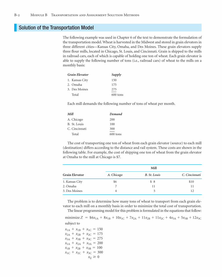
The following example was used in Chapter 6 of the text to demonstrate the formulation ofthe transportation model. Wheat is harvested in the Midwest and stored in grain elevators inthree different cities—Kansas City, Omaha, and Des Moines. These grain elevators supplythree flour mills, located in Chicago, St. Louis, and Cincinnati. Grain is shipped to the millsin railroad cars, each of which is capable of holding one ton of wheat. Each grain elevator isable to supply the following number of tons (i.e., railroad cars) of wheat to the mills on amonthly basis:

Each mill demands the following number of tons of wheat per month.

B-2 Module B Transportation and Assignment Solution Methods

The cost of transporting one ton of wheat from each grain elevator (source) to each mill(destination) differs according to the distance and rail system. These costs are shown in thefollowing table. For example, the cost of shipping one ton of wheat from the grain elevatorat Omaha to the mill at Chicago is $7.

The problem is to determine how many tons of wheat to transport from each grain ele-vator to each mill on a monthly basis in order to minimize the total cost of transportation.

The linear programming model for this problem is formulated in the equations that follow:

subject to

xij Ú 0x1C + x2C + x3C = 300x1B + x2B + x3B = 100x1A + x2A + x3A = 200x3A + x3B + x3C = 275x2A + x2B + x2C = 175x1A + x1B + x1C = 150

minimize Z = $6x1A + 8x1B + 10x1C + 7x2A + 11x2B + 11x2C + 4x3A + 5x3B + 12x3C

Grain Elevator Supply

1. Kansas City 150

2. Omaha 175

3. Des Moines 275

Total 600 tons

Mill Demand

A. Chicago 200

B. St. Louis 100

C. Cincinnati 300

Total 600 tons

Mill

Grain Elevator A. Chicago B. St. Louis C. Cincinnati

1. Kansas City $6 $ 8 $10

2. Omaha 7 11 11

3. Des Moines 4 5 12


Solution of the Transportation Model B-3

Each cell in a transportation tableauis analogous to a decision variable

that indicates the amount allocatedfrom a source to a destination.

In this model the decision variables, , represent the number of tons of wheat trans-ported from each grain elevator, i (where ), to each mill, j (where ).The objective function represents the total transportation cost for each route. Each term inthe objective function reflects the cost of the tonnage transported for one route. For exam-ple, if 20 tons are transported from elevator 1 to mill A, the cost of $6 is multiplied by

which equals $120.The first three constraints in the linear programming model represent the supply at each

elevator; the last three constraints represent the demand at each mill. As an example, con-sider the first supply constraint, This constraint represents thetons of wheat transported from Kansas City to all three mills: Chicago St. Louis

and Cincinnati The amount transported from Kansas City is limited to the 150tons available. Note that this constraint (as well as all others) is an equation rather thana inequality because all the tons of wheat available will be needed to meet the totaldemand of 600 tons. In other words, the three mills demand 600 total tons, which is theexact amount that can be supplied by the three grain elevators. Thus, all that can be sup-plied will be, in order to meet demand. This type of model, in which supply exactly equalsdemand, is referred to as a balanced transportation model. The balanced model will be usedto demonstrate the solution of a transportation problem.

Transportation models are solved manually within the context of a tableau, as in the simplex method. The tableau for our wheat transportation model is shown inTable B-1.

…

(=)(x1C).(x1B),

(x1A),x1A + x1B + x1C = 150.

x1A(=20),

j = A, B, Ci = 1, 2, 3xij

Table B-1The Transportation Tableau

ToFrom A B C Supply

6 8 10

1 150

7 11 11

2 175

4 5 12

3 275

Demand 200 100 300 600

Each cell in the tableau represents the amount transported from one source to one des-tination. Thus, the amount placed in each cell is the value of a decision variable for that cell.For example, the cell at the intersection of row 1 and column A represents the decision vari-able The smaller box within each cell contains the unit transportation cost for thatroute. For example, in cell 1A the value, $6, is the cost of transporting one ton of wheatfrom Kansas City to Chicago. Along the outer rim of the tableau are the supply and demandconstraint quantity values, which are referred to as rim requirements.

The two methods for solving a transportation model are the stepping-stone method andthe modified distribution method (also known as MODI). In applying the simplex method,an initial solution had to be established in the initial simplex tableau. This same conditionmust be met in solving a transportation model. In a transportation model, an initial feasi-ble solution can be found by several alternative methods, including the northwest cornermethod, the minimum cell cost method, and Vogel’s approximation model.

x1A.

Transportation models do not startat the origin where all decision

variables equal zero; they must begiven an initial feasible solution.

The supply and demand valuesalong the outside rim of a tableau

are called rim requirements.

Transportation problems aresolved manually within a tableau

format.



The Northwest Corner MethodWith the northwest corner method, an initial allocation is made to the cell in the upperleft-hand corner of the tableau (i.e., the “northwest corner”). The amount allocated is themost possible, subject to the supply and demand constraints for that cell. In our example,we first allocate as much as possible to cell 1A (the northwest corner). This amount is 150tons, since that is the maximum that can be supplied by grain elevator 1 at Kansas City,even though 200 tons are demanded by mill A at Chicago. This initial allocation is shown inTable B-2.

We next allocate to a cell adjacent to cell 1A, in this case either cell 2A or cell 1B.However, cell 1B no longer represents a feasible allocation, because the total tonnage ofwheat available at source 1 (i.e., 150 tons) has already been allocated. Thus, cell 2A repre-sents the only feasible alternative, and as much as possible is allocated to this cell. Theamount allocated at 2A can be either 175 tons, the supply available from source 2 (Omaha),or 50 tons, the amount now demanded at destination A. (Recall that 150 of the 200 tonsdemanded at A have already been supplied.) Because 50 tons is the most constrainedamount, it is allocated to cell 2A, as shown in Table B-2.

In the northwest corner methodthe largest possible allocation is

made to the cell in the upper left-hand corner of the tableau,

followed by allocations to adjacentfeasible cells.

Table B-2The Initial NW Corner Solution

ToFrom A B C Supply

6 8 10

1 150 150

7 11 11

2 50 100 25 175

4 5 12

3 275 275

Demand 200 100 300 600

The third allocation is made in the same way as the second allocation. The only feasiblecell adjacent to cell 2A is cell 2B. The most that can be allocated is either 100 tons (theamount demanded at mill B) or 125 tons (175 tons minus the 50 tons allocated to cell 2A).The smaller (most constrained) amount, 100 tons, is allocated to cell 2B, as shown inTable B-2.

The fourth allocation is 25 tons to cell 2C, and the fifth allocation is 275 tons to cell 3C,both of which are shown in Table B-2. Notice that all of the row and column allocationsadd up to the appropriate rim requirements.

The transportation cost of this solution is computed by substituting the cell allocations(i.e., the amounts transported),

into the objective function:

= $5,925 = 6(150) + 8(0) + 10(0) + 7(50) + 11(100) + 11(25) + 4(0) + 5(0) + 12(275)

Z = $6x1A + 8x1B + 10x1C + 7x2A + 11x2B + 11x2C + 4x3A + 5x3B + 12x3C

x3C = 275 x2C = 25 x2B = 100 x2A = 50 x1A = 150

The initial solution is completewhen all rim requirements are

satisfied.


The steps of the northwest corner method are summarized here:

1. Allocate as much as possible to the cell in the upper left-hand corner, subject to thesupply and demand constraints.

2. Allocate as much as possible to the next adjacent feasible cell.3. Repeat step 2 until all rim requirements have been met.

The Minimum Cell Cost MethodWith the minimum cell cost method, the basic logic is to allocate to the cells with the low-est costs. The initial allocation is made to the cell in the tableau having the lowest cost. Inthe transportation tableau for our example problem, cell 3A has the minimum cost of $4.As much as possible is allocated to this cell; the choice is either 200 tons or 275 tons. Eventhough 275 tons could be supplied to cell 3A, the most we can allocate is 200 tons, sinceonly 200 tons are demanded. This allocation is shown in Table B-3.


Table B-3The Initial Minimum Cell

Cost Allocation

ToFrom A B C Supply

6 8 10

1 150

7 11 11

2 175

4 5 12

3 200 275

Demand 200 100 300 600

Table B-4The Second Minimum Cell

Cost Allocation

ToFrom A B C Supply

6 8 10

1 150

7 11 11

2 175

4 5 12

3 200 75 275

Demand 200 100 300 600

Notice that all the remaining cells in column A have now been eliminated, because allthe wheat demanded at destination A, Chicago, has now been supplied by source 3, DesMoines.

The next allocation is made to the cell that has the minimum cost and also is feasible.This is cell 3B, which has a cost of $5. The most that can be allocated is 75 tons (275 tonsminus the 200 tons already supplied). This allocation is shown in Table B-4.

In the minimum cell cost methodas much as possible is allocated to

the cell with the minimum cost.


The third allocation is made to cell 1B, which has the minimum cost of $8. (Notice thatcells with lower costs, such as 1A and 2A, are not considered because they were previouslyruled out as infeasible.) The amount allocated is 25 tons. The fourth allocation of 125 tonsis made to cell 1C, and the last allocation of 175 tons is made to cell 2C. These allocations,which complete the initial minimum cell cost solution, are shown in Table B-5.


Table B-5The Initial Solution

ToFrom A B C Supply

6 8 10

1 25 125 150

7 11 11

2 175 175

4 5 12

3 200 75 275

Demand 200 100 300 600

The total cost of this initial solution is $4,550, as compared with a total cost of $5,925 forthe initial northwest corner solution. It is not a coincidence that a lower total cost is derivedusing the minimum cell cost method; it is a logical occurrence. The northwest cornermethod does not consider cost at all in making allocations—the minimum cell costmethod does. It is therefore quite natural that a lower initial cost will be attained using thelatter method. Thus, the initial solution achieved by using the minimum cell cost method isusually better in that, because it has a lower cost, it is closer to the optimal solution; fewersubsequent iterations will be required to achieve the optimal solution.

The specific steps of the minimum cell cost method are summarized next:

1. Allocate as much as possible to the feasible cell with the minimum transportationcost, and adjust the rim requirements.

2. Repeat step 1 until all rim requirements have been met.

Vogel’s Approximation ModelThe third method for determining an initial solution, Vogel’s approximation model (alsocalled VAM), is based on the concept of penalty cost or regret. If a decision maker incor-rectly chooses from several alternative courses of action, a penalty may be suffered (and thedecision maker may regret the decision that was made). In a transportation problem, thecourses of action are the alternative routes, and a wrong decision is allocating to a cell thatdoes not contain the lowest cost.

In the VAM method, the first step is to develop a penalty cost for each source and desti-nation. For example, consider column A in Table B-6. Destination A, Chicago, can be sup-plied by Kansas City, Omaha, and Des Moines. The best decision would be to supplyChicago from source 3 because cell 3A has the minimum cost of $4. If a wrong decision wasmade and the next higher cost of $6 was selected at cell 1A, a “penalty” of $2 per ton wouldresult (i.e., ). This demonstrates how the penalty cost is determined for eachrow and column of the tableau. The general rule for computing a penalty cost is to subtractthe minimum cell cost from the next higher cell cost in each row and column. The penaltycosts for our example are shown at the right and at the bottom of Table B-6.

$6 - 4 = $2

A penalty cost is the differencebetween the largest and

next largest cell cost in a row (or column).

VAM allocates as much as possibleto the minimum cost cell in therow or column with the largest

penalty cost.

The minimum cell cost methodwill provide a solution with alower cost than the northwest

corner solution because itconsiders cost in the

allocation process.



The initial allocation in the VAM method is made in the row or column that has thehighest penalty cost. In Table B-6, row 2 has the highest penalty cost of $4. We allocate asmuch as possible to the feasible cell in this row with the minimum cost. In row 2, cell 2Ahas the lowest cost of $7, and the most that can be allocated to cell 2A is 175 tons. With thisallocation the greatest penalty cost of $4 has been avoided because the best course of actionhas been selected. The allocation is shown in Table B-7.

Table B-6The VAM Penalty Costs

ToFrom A B C Supply

6 8 102

1 150

7 11 114

2 175

4 5 121

3 275

Demand 200 100 300 600

2 3 1

Table B-7The Initial VAM Allocation

ToFrom A B C Supply

6 8 102

1 150

7 11 11

2 175 175

4 5 121

3 275

Demand 200 100 300 600

2 3 2

After the initial allocation is made, all the penalty costs must be recomputed. In somecases the penalty costs will change; in other cases they will not change. For example, thepenalty cost for column C in Table B-7 changed from $1 to $2 (because cell 2C is no longerconsidered in computing penalty cost), and the penalty cost in row 2 was eliminated alto-gether (because no more allocations are possible for that row).

Next, we repeat the previous step and allocate to the row or column with the highestpenalty cost, which is now column B with a penalty cost of $3 (see Table B-7). The cell incolumn B with the lowest cost is 3B, and we allocate as much as possible to this cell, 100tons. This allocation is shown in Table B-8.

Note that all penalty costs have been recomputed in Table B-8. Since the highest penaltycost is now $8 for row 3 and since cell 3A has the minimum cost of $4, we allocate 25 tonsto this cell, as shown in Table B-9.

After each VAM cell allocation,all row and column penalty costs

are recomputed.



Table B-9 also shows the recomputed penalty costs after the third allocation. Notice thatby now only column C has a penalty cost. Rows 1 and 3 have only one feasible cell, so apenalty does not exist for these rows. Thus, the last two allocations are made to column C.First, 150 tons are allocated to cell 1C because it has the lowest cell cost. This leaves only cell3C as a feasible possibility, so 150 tons are allocated to this cell. Both of these allocations areshown in Table B-10.

Table B-8The Second VAM Allocation

ToFrom A B C Supply

6 8 104

1 150

7 11 11

2 175 175

4 5 128

3 100 275

Demand 200 100 300 600

2 2

Table B-9The Third VAM Allocation

ToFrom A B C Supply

6 8 10

1 150

7 11 11

2 175 175

4 5 12

3 25 100 275

Demand 200 100 300 600

2

Table B-10The Initial VAM Solution

ToFrom A B C Supply

6 8 10

1 150 150

7 11 11

2 175 175

4 5 12

3 25 100 150 275

Demand 200 100 300 600


The basic solution principle in a transportation problem is to determine whether atransportation route not at present being used (i.e., an empty cell) would result in alower total cost if it were used. For example, Table B-11 shows four empty cells (1A, 2A,2B, and 3C) representing unused routes. Our first step in the stepping-stone method is toevaluate these empty cells to see whether the use of any of them would reduce total cost.If we find such a route, then we will allocate as much as possible to it.

First, let us consider allocating one ton of wheat to cell 1A. If one ton is allocated tocell 1A, cost will be increased by $6—the transportation cost for cell 1A. However, byallocating one ton to cell 1A, we increase the supply in row 1 to 151 tons, as shown inTable B-12.


The total cost of this initial Vogel’s approximation model solution is $5,125, which isnot as high as the northwest corner initial solution of $5,925. It is also not as low as theminimum cell cost solution of $4,550. Like the minimum cell cost method, VAM typi-cally results in a lower cost for the initial solution than does the northwest cornermethod.

The steps of Vogel’s approximation model can be summarized in the following list:

1. Determine the penalty cost for each row and column by subtracting the lowest cellcost in the row or column from the next lowest cell cost in the same row or column.

2. Select the row or column with the highest penalty cost (breaking ties arbitrarily orchoosing the lowest-cost cell).

3. Allocate as much as possible to the feasible cell with the lowest transportation cost inthe row or column with the highest penalty cost.

4. Repeat steps 1, 2, and 3 until all rim requirements have been met.

The Stepping-Stone Solution MethodOnce an initial basic feasible solution has been determined by any of the previous threemethods, the next step is to solve the model for the optimal (i.e., minimum total cost) solu-tion. There are two basic solution methods: the stepping-stone solution method and themodified distribution method (MODI). The stepping-stone solution method will bedemonstrated first. Because the initial solution obtained by the minimum cell cost methodhad the lowest total cost of the three initial solutions, we will use it as the starting solution.Table B-11 repeats the initial solution that was developed from the minimum cell costmethod.

Table B-11The Minimum Cell

Cost Solution

ToFrom A B C Supply

6 8 10

1 25 125 150

7 11 11

2 175 175

4 5 12

3 200 75 275

Demand 200 100 300 600

VAM and minimum cell cost bothprovide better initial solutions

than the northwest corner method.

The stepping-stone methoddetermines whether there is a cell

with no allocation that wouldreduce cost if used.

Once an initial solution is derived,the problem must be solved using

either the stepping-stone methodor the modified distribution

method (MODI).


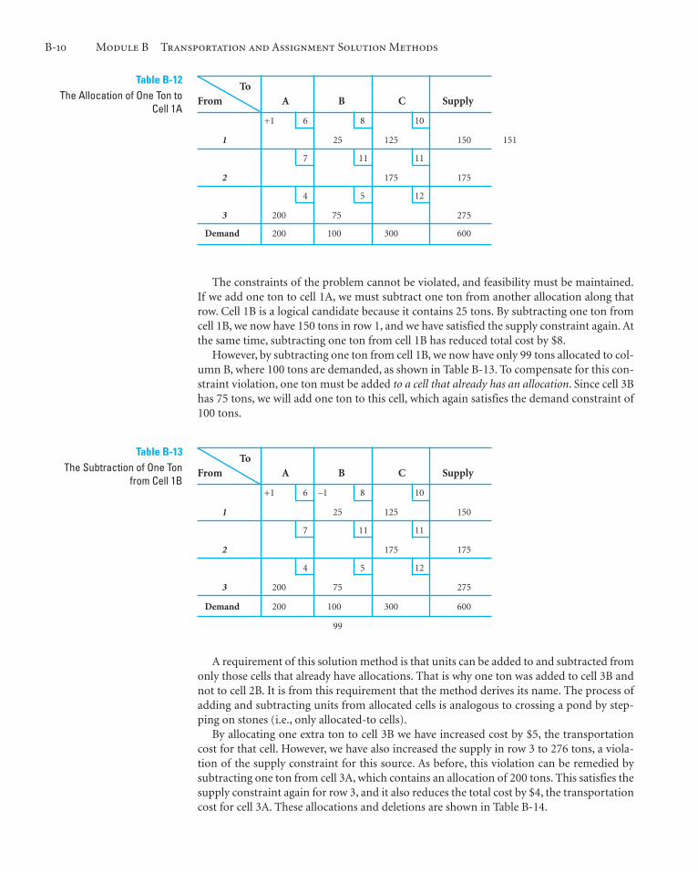
The constraints of the problem cannot be violated, and feasibility must be maintained.If we add one ton to cell 1A, we must subtract one ton from another allocation along thatrow. Cell 1B is a logical candidate because it contains 25 tons. By subtracting one ton fromcell 1B, we now have 150 tons in row 1, and we have satisfied the supply constraint again. Atthe same time, subtracting one ton from cell 1B has reduced total cost by $8.

However, by subtracting one ton from cell 1B, we now have only 99 tons allocated to col-umn B, where 100 tons are demanded, as shown in Table B-13. To compensate for this con-straint violation, one ton must be added to a cell that already has an allocation. Since cell 3Bhas 75 tons, we will add one ton to this cell, which again satisfies the demand constraint of100 tons.


Table B-12The Allocation of One Ton to

Cell 1A

ToFrom A B C Supply

+1 6 8 10

1 25 125 150 151

7 11 11

2 175 175

4 5 12

3 200 75 275

Demand 200 100 300 600

Table B-13The Subtraction of One Ton

from Cell 1B

ToFrom A B C Supply

+1 6 –1 8 10

1 25 125 150

7 11 11

2 175 175

4 5 12

3 200 75 275

Demand 200 100 300 600

99

A requirement of this solution method is that units can be added to and subtracted fromonly those cells that already have allocations. That is why one ton was added to cell 3B andnot to cell 2B. It is from this requirement that the method derives its name. The process ofadding and subtracting units from allocated cells is analogous to crossing a pond by step-ping on stones (i.e., only allocated-to cells).

By allocating one extra ton to cell 3B we have increased cost by $5, the transportationcost for that cell. However, we have also increased the supply in row 3 to 276 tons, a viola-tion of the supply constraint for this source. As before, this violation can be remedied bysubtracting one ton from cell 3A, which contains an allocation of 200 tons. This satisfies thesupply constraint again for row 3, and it also reduces the total cost by $4, the transportationcost for cell 3A. These allocations and deletions are shown in Table B-14.


Notice in Table B-14 that by subtracting one ton from cell 3A, we did not violate thedemand constraint for column A, since we previously added one ton to cell 1A.

Now let us review the increases and reductions in costs resulting from this process. Weinitially increased cost by $6 at cell 1A, then reduced cost by $8 at cell 1B, then increasedcost by $5 at cell 3B, and, finally, reduced cost by $4 at cell 3A:

In other words, for each ton allocated to cell 1A (a route not at present used), total costwill be reduced by $1. This indicates that the initial solution is not optimal because a lowercost can be achieved by allocating additional tons of wheat to cell 1A (i.e., cell 1A is analo-gous to a pivot column in the simplex method). Our goal is to determine the cell or enter-ing “variable” that will reduce cost the most. Another variable (empty cell) may result in aneven greater decrease in cost than cell 1A. If such a cell exists, it will be selected as the enter-ing variable; if not, cell 1A will be selected. To identify the appropriate entering variable, theremaining empty cells must be tested as cell 1A was.

Before testing the remaining empty cells, let us identify a few of the general characteris-tics of the stepping-stone process. First, we always start with an empty cell and form a closedpath of cells that now have allocations. In developing the path, it is possible to skip overboth unused and used cells. In any row or column there can be only one addition and onesubtraction. (For example, in row 1, wheat is added at cell 1A and is subtracted at cell 1B.)

Let us test cell 2A to see if it results in a cost reduction. The stepping-stone closed pathfor cell 2A is shown in Table B-15. Notice that the path for cell 2A is slightly more complex

+ $6 - 8 + 5 - 4 = - $11A : 1B : 3B : 3A


Table B-15The Stepping-Stone Path for

Cell 2A

ToFrom A B C Supply

6 – 8 + 10

1 25 125 150

+ 7 11 – 11

2 175 175

– 4 + 5 12

3 200 75 275

Demand 200 100 300 600

+ $7 - 11 + 10 - 8 + 5 - 4 = - $12A : 2C : 1C : 1B : 3B : 3A

Table B-14The Addition of One Ton to Cell3B and the Subtraction of One

Ton from Cell 3A

ToFrom A B C Supply

+1 6 –1 8 10

1 25 125 150

7 11 11

2 175 175

–1 4 +1 5 12

3 200 75 275

Demand 200 100 300 600

To evaluate the cost reductionpotential of an empty cell, a closed

path connecting used cells to theempty cell is identified.

An empty cell that will reduce costis a potential entering variable.



than the path for cell 1A. Notice also that the path crosses itself at one point, which is per-fectly acceptable. An allocation to cell 2A will reduce cost by $1, as shown in the computa-tion in Table B-15. Thus, we have located another possible entering variable, although it isno better than cell 1A.

The remaining stepping-stone paths and the resulting computations for cells 2B and 3Care shown in Tables B-16 and B-17, respectively.


Cell 2B

ToFrom A B C Supply

6 8 10

1 25 125 150

7 11 11

2 175 175

4 5 12

3 200 75 275

Demand 200 100 300 600

+ $11 - 11 + 10 - 8 = + $22B : 2C : 1C : 1B

+-

-+


Cell 3C

ToFrom A B C Supply

6 8 10

1 25 125 150

7 11 11

2 175 175

4 5 12

3 200 75 275

Demand 200 100 300 600

+ $12 - 10 + 8 - 5 = + $53C : 1C : 1B : 3B

+-

-+

Notice that after all four unused routes are evaluated, there is a tie for the entering vari-able between cells 1A and 2A. Both show a reduction in cost of $1 per ton allocated to thatroute. The tie can be broken arbitrarily. We will select cell 1A (i.e., ) to enter the solution.

Because the total cost of the model will be reduced by $1 for each ton we can reallocateto cell 1A, we naturally want to reallocate as much as possible. To determine how much toallocate, we need to look at the path for cell 1A again, as shown in Table B-18.

The stepping-stone path in Table B-18 shows that tons of wheat must be subtracted atcells 1B and 3A to meet the rim requirements and thus satisfy the model constraints.Because we cannot subtract more than is available in a cell, we are limited by the 25 tons incell 1B. In other words, if we allocate more than 25 tons to cell 1A, then we must subtractmore than 25 tons from 1B, which is impossible because only 25 tons are available.Therefore, 25 tons is the amount we reallocate to cell 1A according to our path. That is,25 tons are added to 1A, subtracted from 1B, added to 3B, and subtracted from 3A. Thisreallocation is shown in Table B-19.

x1A

After all empty cells are evaluated,the one with the greatest

cost reduction potential is theentering variable.

When reallocating units to theentering variable (cell), the

amount is the minimumamount subtracted on the

stepping-stone path.



The process culminating in Table B-19 represents one iteration of the stepping-stonemethod. We selected as the entering variable, and it turned out that was the leavingvariable (because it now has a value of zero in Table B-19). Thus, at each iteration one vari-able enters and one leaves (just as in the simplex method).

Now we must check to see whether the solution shown in Table B-19 is, in fact, optimal.We do this by plotting the paths for the unused routes (i.e., empty cells 2A, 1B, 2B, and 3C)that are shown in Table B-19. These paths are shown in Tables B-20 through B-23.

x1Bx1A


Cell 1A

ToFrom A B C Supply

6 8 10

1 25 125 150

7 11 11

2 175 175

4 5 12

3 200 75 275

Demand 200 100 300 600

+-

-+

Table B-19The Second Iteration of the

Stepping-Stone Method

ToFrom A B C Supply

6 8 10

1 25 125 150

7 11 11

2 175 175

4 5 12

3 175 100 275

Demand 200 100 300 600


Cell 2A

ToFrom A B C Supply

6 8 10

1 25 125 150

7 11 11

2 175 175

4 5 12

3 175 100 275

Demand 200 100 300 600

+ $7 - 11 + 10 - 6 = $02A : 2C : 1C : 1A

-+

+-



Our evaluation of the four paths indicates no cost reductions; therefore, the solutionshown in Table B-19 is optimal. The solution and total minimum cost are

= $4,525 Z = $6(25) + 8(0) + 10(125) + 7(0) + 11(0) + 11(175) + 4(175) + 5(100) + 12(0)

x3B = 100 tons x1C = 125 tonsx3A = 175 tonsx2C = 175 tons x1A = 25 tons

The stepping-stone process isrepeated until none of the

empty cells will reduce cost(i.e., an optimal solution).


Cell 1B

ToFrom A B C Supply

6 8 10

1 25 125 150

7 11 11

2 175 175

4 5 12

3 175 100 275

Demand 200 100 300 600

+ $8 - 5 + 4 - 6 = + $11B : 3B : 3A : 1A

-+

+-


Cell 2B

ToFrom A B C Supply

6 8 10

1 25 125 150

7 11 11

2 175 175

4 5 12

3 175 100 275

Demand 200 100 300 600

+ $11 - 5 + 4 - 6 + 10 - 11 = + $32B : 3B : 3A : 1A : 1C : 2C

-+

-+

+-


Cell 3C

ToFrom A B C Supply

6 8 10

1 25 125 150

7 11 11

2 175 175

4 5 12

3 175 100 275

Demand 200 100 300 600

+ $12 - 4 + 6 - 10 = + $43C : 3A : 1A : 1C

+-

-+



However, notice in Table B-20 that the path for cell 2A resulted in a cost change of $0. Inother words, allocating to this cell would neither increase nor decrease total cost. This situ-ation indicates that the problem has multiple optimal solutions. Thus, could beentered into the solution and there would not be a change in the total minimum cost of$4,525. To identify the alternative solution, we would allocate as much as possible to cell 2A,which in this case is 25 tons of wheat. The alternative solution is shown in Table B-24.

x2A

Multiple optimal solutionsoccur when an empty cell has a

cost change of zero and all otherempty cells are positive.

An alternative optimal solution isdetermined by allocating to the

empty cell a zero cost change.

Table B-24The Alternative Optimal

Solution

ToFrom A B C Supply

6 8 10

1 150 150

7 11 11

2 25 150 175

4 5 12

3 175 100 275

Demand 200 100 300 600

Table B-25The Minimum Cell Cost

Initial SolutionTo

From A B C Supply

6 8 10

1 25 125 150

7 11 11

2 175 175

4 5 12

3 200 75 275

Demand 200 100 300 600

u3 =

u2 =

u1 =

ui

vC =vB =vA =vj

The solution in Table B-24 also results in a total minimum cost of $4,525. The steps ofthe stepping-stone method are summarized here:

1. Determine the stepping-stone paths and cost changes for each empty cell in thetableau.

2. Allocate as much as possible to the empty cell with the greatest net decrease in cost.3. Repeat steps 1 and 2 until all empty cells have positive cost changes that indicate an

optimal solution.

The Modified Distribution MethodThe modified distribution method (MODI) is basically a modified version of the stepping-stone method. However, in the MODI method the individual cell cost changes are deter-mined mathematically, without identifying all the stepping-stone paths for the empty cells.

To demonstrate MODI, we will again use the initial solution obtained by the minimumcell cost method. The tableau for the initial solution with the modifications required byMODI is shown in Table B-25.

MODI is a modified version ofthe stepping-stone method in

which math equations replace thestepping-stone paths.



The extra left-hand column with the symbols and the extra top row with the sym-bols represent column and row values that must be computed in MODI. These values arecomputed for all cells with allocations by using the following formula:

The value is the unit transportation cost for cell ij. For example, the formula for cell 1B is

and, since

The formulas for the remaining cells that presently contain allocations are

Now there are five equations with six unknowns. To solve these equations, it is necessaryto assign only one of the unknowns a value of zero. Thus, if we let we can solve forall remaining and values.

Notice that the equation for cell 3B had to be solved before the cell 3A equation could besolved. Now all the and values can be substituted into the tableau, as shown in Table B-26.vjui

vA = 7 -3 + vA = 4

x3A: u3 + vA = 4 u3 = -3

u3 + 8 = 5 x3B: u3 + vB = 5

u2 = 1 u2 + 10 = 11

x2C: u2 + vC = 11 vC = 10

0 + vC = 10 x1C: u1 + vC = 10

vB = 8 0 + vB = 8

x1B: u1 + vB = 8

vjui

u1 = 0,

x3B: u3 + vB = 5 x3A: u3 + vA = 4 x2C: u2 + vC = 11 x1C: u1 + vC = 10

u1 + vB = 8

c1B = 8,

u1 + vB = c1B

cij

ui + vj = cij

vjui

Table B-26The Initial Solution with All

and Valuesvj

ui ToFrom A B C Supply

6 8 10

1 25 125 150

7 11 11

2 175 175

4 5 12

3 200 75 275

Demand 200 100 300 600

u3 = -3

u2 = 1

u1 = 0

ui

vC = 10vB = 8vA = 7vj


Next, we use the following formula to evaluate all empty cells:

where equals the cost increase or decrease that would occur by allocating to a cell.For the empty cells in Table B-26, the formula yields the following values:

These calculations indicate that either cell 1A or cell 2A will decrease cost by $1 per allo-cated ton. Notice that those are exactly the same cost changes for all four empty cells aswere computed in the stepping-stone method. That is, the same information is obtained byevaluating the paths in the stepping-stone method and by using the mathematical formulasof the MODI.

We can select either cell 1A or 2A to allocate to because they are tied at If cell 1A isselected as the entering nonbasic variable, then the stepping-stone path for that cell mustbe determined so that we know how much to reallocate. This is the same path previouslyidentified in Table B-18. Reallocating along this path results in the tableau shown inTable B-27 (and previously shown in Table B-19).

-1.

x3C: k3C = c3C - u3 - vC = 12 - (-3) - 10 = +5 x2B: k2B = c2B - u2 - vB = 11 - 1 - 8 = +2 x2A: k2A = c2A - u2 - vA = 7 - 1 - 7 = -1 x1A: k1A = c1A - u1 - vA = 6 - 0 - 7 = -1

kij

cij - ui - vj = kij


Each MODI allocation replicatesthe stepping-stone allocation.

After each allocation to an emptycell, the and values must be

recomputed.vjui

Table B-27The Second Iteration of the

MODI Solution MethodTo

From A B C Supply

6 8 10

1 25 125 150

7 11 11

2 175 175

4 5 12

3 175 100 275

Demand 200 100 300 600

u3 =

u2 =

u1 =

ui

vC =vB =vA =vj

The and values for Table B-27 must now be recomputed using our formula for theallocated-to cells:

vB = 7 -2 + vB = 5

x3B: u3 + vB = 5 u3 = -2

u3 + 6 = 4 x3A: u3 + vA = 4

u2 = 1 u2 + 10 = 11

x2C: u2 + vC = 11 vC = 10

0 + vC = 10 x1C: u1 + vC = 10

vA = 6 0 + vA = 6

x1A: u1 + vA = 6

vjui


The cost changes for the empty cells are now computed using the formula

Because none of these values is negative, the solution shown in Table B-28 is optimal.However, as in the stepping-stone method, cell 2A with a zero cost change indicates multi-ple optimal solutions.

The steps of the modified distribution method can be summarized as follows:

1. Develop an initial solution using one of the three methods available.2. Compute and values for each row and column by applying the formula

to each cell that has an allocation.3. Compute the cost change, for each empty cell using 4. Allocate as much as possible to the empty cell that will result in the greatest net

decrease in cost (most negative ). Allocate according to the stepping-stone path forthe selected cell.

5. Repeat steps 2 through 4 until all values are positive or zero.

The Unbalanced Transportation ModelThus far, the methods for determining an initial solution and an optimal solution havebeen demonstrated within the context of a balanced transportation model. Realistically,however, an unbalanced problem is a more likely occurrence. Consider our example oftransporting wheat. By changing the demand at Cincinnati to 350 tons, we create a situa-tion in which total demand is 650 tons and total supply is 600 tons.

To compensate for this difference in the transportation tableau, a “dummy”row is addedto the tableau, as shown in Table B-29. The dummy row is assigned a supply of 50 tonsto balance the model. The additional 50 tons demanded, which cannot be supplied, willbe allocated to a cell in the dummy row. The transportation costs for the cells in thedummy row are zero because the tons allocated to these cells are not amounts really trans-ported but the amounts by which demand was not met. These dummy cells are, in effect,slack variables.

kij

kij

cij - ui - vj = kij.kij,ui + vj = cij

vjui

x3C: k3C = c3C - u3 - vC = 12 - (-2) - 10 = +4 x2B: k2B = c2B - u2 - vB = 11 - 1 - 7 = +3 x2A: k2A = c2A - u2 - vA = 7 - 1 - 6 = 0 x1B: k1B = c1B - u1 - vB = 8 - 0 - 7 = +1

cij - ui - vj = kij:

These new and values are shown in Table B-28.vjui


When demand exceeds supply,a dummy row is added to the

tableau.

Table B-28The New and Values for

the Second Iterationvjui To

From A B C Supply

6 8 10

1 25 125 150

7 11 11

2 175 175

4 5 12

3 175 100 275

Demand 200 100 300 600

u3 = -2

u2 = 1

u1 = 0

ui

vC = 10vB = 7vA = 6vj


Now consider our example with the supply at Des Moines increased to 375 tons. Thisincreases total supply to 700 tons, while total demand remains at 600 tons. To compensate forthis imbalance, we add a dummy column instead of a dummy row, as shown in Table B-30.


Table B-29An Unbalanced Model

(Demand Supply)7

ToFrom A B C Supply

6 8 10

1 150

7 11 11

2 175

4 5 12

3 275

0 0 0

Dummy 50

Demand 200 100 350 650

Table B-30An Unbalanced Model

(Supply Demand)7

ToFrom A B C Dummy Supply

6 8 10 0

1 150

7 11 11 0

2 175

4 5 12 0

3 375

Demand 200 100 300 100 700

When a supply exceeds demand,a dummy column is added to the

tableau.

The addition of a dummy row or a dummy column has no effect on the initial solutionmethods or on the methods for determining an optimal solution. The dummy row or col-umn cells are treated the same as any other tableau cell. For example, in the minimum cellcost method, three cells would be tied for the minimum cost cell, each with a cost of zero.In this case (or any time there is a tie between cells) the tie would be broken arbitrarily.

DegeneracyIn all the tableaus showing a solution to the wheat transportation problem, the followingcondition was met:

For example, in any of the balanced tableaus for wheat transportation, the number ofrows was three (i.e., ) and the number of columns was three (i.e., ); thus,

cells with allocations.These tableaus always had five cells with allocations; thus, our condition for normal

solution was met. When this condition is not met and fewer than cells haveallocations, the tableau is said to be degenerate.

m + n - 1

3 + 3 - 1 = 5n = 3m = 3

m rows + n columns - 1 = the number of cells with allocations

In a transportation tableau with m rows and n columns, there

must be cells withallocations; if not, it is degenerate.

m + n - 1


Consider the wheat transportation example with the supply values changed to theamounts shown in Table B-31. The initial solution shown in this tableau was developedusing the minimum cell cost method.


The tableau shown in Table B-31 does not meet the condition

because there are only four cells with allocations. The difficulty resulting from a degeneratesolution is that neither the stepping-stone method nor MODI will work unless the preced-ing condition is met (there is an appropriate number of cells with allocations). When thetableau is degenerate, a closed path cannot be completed for all cells in the stepping-stonemethod, and not all the computations can be completed in MODI. For exam-ple, a closed path cannot be determined for cell 1A in Table B-31.

To create a closed path, one of the empty cells must be artificially designated as a cellwith an allocation. Cell 1A in Table B-32 is designated arbitrarily as a cell with artificialallocation of zero. (However, any symbol, such as could be used to signify the artificialallocation.) This indicates that this cell will be treated as a cell with an allocation in deter-mining stepping-stone paths or MODI formulas, although there is no real allocation in thiscell. Notice that the location of 0 was arbitrary because there is no general rule for allocat-ing the artificial cell. Allocating zero to a cell does not guarantee that all the stepping-stonepaths can be determined.

�,

ui + vj = cij

3 + 3 - 1 = 5 cells m + n - 1 = the number of cells with allocations

Table B-31The Minimum Cell Cost Initial

Solution

ToFrom A B C Supply

6 8 10

1 100 50 150

7 11 11

2 250 250

4 5 12

3 200 200

Demand 200 100 300 600

Table B-32The Initial Solution

ToFrom A B C Supply

6 8 10

1 0 100 50 150

7 11 11

2 250 250

4 5 12

3 200 200

Demand 200 100 300 600

In a degenerate tableau, not all ofthe stepping-stone paths or MODI

equations can be developed.

To rectify a degenerate tableau, anempty cell must artificially be

treated as an occupied cell.



For example, if zero had been allocated to cell 2B instead of to cell 1A, none of thestepping-stone paths could have been determined, even though technically the tableauwould no longer be degenerate. In such a case, the zero must be reallocated to another celland all paths determined again. This process must be repeated until an artificial allocationhas been made that will enable the determination of all paths. In most cases, however, thereis more than one possible cell to which such an allocation can be made.

The stepping-stone paths and cost changes for this tableau follow:

Because cell 3B shows a $1 decrease in cost for every ton of wheat allocated to it, we willallocate 100 tons to cell 3B. This results in the tableau shown in Table B-33.

x3C: 12 - 10 + 6 - 4 = +4 3C 1C 1A 3A

x3B: 5 - 8 + 6 - 4 = -1 3B 1B 1A 3A

x2B: 11 - 11 + 10 - 8 = +2 2B 2C 1C 1B

x2A: 7 - 11 + 10 - 6 = 0 2A 2C 1C 1A

Table B-33The Second Stepping-Stone

Iteration

ToFrom A B C Supply

6 8 10

1 100 50 150

7 11 11

2 250 250

4 5 12

3 100 100 200

Demand 200 100 300 600

Notice that the solution in Table B-33 now meets the condition Thus,in applying the stepping-stone method (or MODI) to this tableau, it is not necessary tomake an artificial allocation to an empty cell. It is quite possible to begin the solution processwith a normal tableau and have it become degenerate or begin with a degenerate tableau andhave it become normal. If it had been indicated that the cell with the zero should have unitssubtracted from it, no actual units could have been subtracted. In that case the zero wouldhave been moved to the cell that represents the entering variable. (The solution shown inTable B-33 is optimal; however, multiple optimal solutions exist at cell 2A.)

Prohibited RoutesSometimes one or more of the routes in the transportation model are prohibited. That is,units cannot be transported from a particular source to a particular destination. When thissituation occurs, we must make sure that no units in the optimal solution are allocated tothe cell representing this route. In our study of the simplex tableau, we learned that assign-ing a large relative cost or a coefficient of M to a variable would keep it out of the final solu-tion. This same principle can be used in a transportation model for a prohibited route. Avalue of M is assigned as the transportation cost for a cell that represents a prohibitedroute. Thus, when the prohibited cell is evaluated, it will always contain a large positive costchange of M, which will keep it from being selected as an entering variable.

m + n - 1 = 5.A normal problem can becomedegenerate at any iteration and

vice versa.

A prohibited route is assigneda large cost such as M so that itwill never receive an allocation.



The supply is always one team of officials, and the demand is for only one team of offi-cials at each game. Table B-34 is already in the proper form for the assignment.

The first step in the assignment method of solution is to develop an opportunity costtable. We accomplish this by first subtracting the minimum value in each row from everyvalue in the row. These computations are referred to as row reductions. We applied a similarprinciple in the VAM method when we determined penalty costs. In other words, the bestcourse of action is determined for each row, and the penalty or “lost opportunity” is devel-oped for all other row values. The row reductions for this example are shown in Table B-35.

Solution of the Assignment Model

The assignment model is a special form of a linear programming model that is similar tothe transportation model. There are differences, however. In the assignment model, thesupply at each source and the demand at each destination are limited to one unit each.

The following example from the text will be used to demonstrate the assignment modeland its special solution method. The Atlantic Coast Conference has four basketball gameson a particular night. The conference office wants to assign four teams of officials to thefour games in a way that will minimize the total distance traveled by the officials. The dis-tances in miles for each team of officials to each game location are shown in Table B-34.

An assignment model is a specialform of the transportation model

in which all supply anddemand values equal one.

Table B-34The Travel Distances to Each

Game for Each Team ofOfficials

Game Sites

Officials RALEIGH ATLANTA DURHAM CLEMSON

A 210 90 180 160B 100 70 130 200C 175 105 140 170D 80 65 105 120

Table B-35The Assignment Tableau with

Row Reductions

Game Sites


A 120 0 90 70B 30 0 60 130C 70 0 35 65D 15 0 40 55

Table B-36The Tableau with

Column Reductions

Game Sites


A 105 0 55 15B 15 0 25 75C 55 0 0 10D 0 0 5 0

An opportunity cost table isdeveloped by first substracting

the minimum value in eachrow from all other row values and

then repeating this process foreach column.

Next, the minimum value in each column is subtracted from all column values. Thesecomputations are called column reductions and are shown in Table B-36, which representsthe completed opportunity cost table for our example. Assignments can be made in thistable wherever a zero is present. For example, team A can be assigned to Atlanta. An optimalsolution results when each of the four teams can be uniquely assigned to a different game.


Solution of the Assignment Model B-23

Assignments are made to locationswith zeros in the opportunity cost

table.

An optimal solution occurs whenthe number of independent uniqueassignments equals the number of

rows or columns.

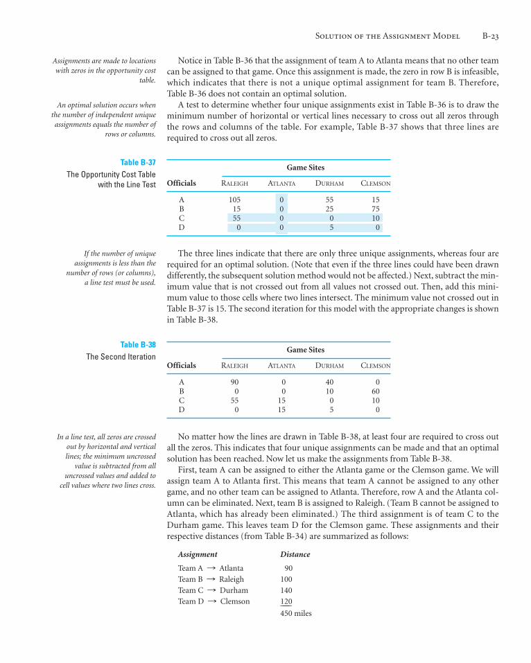
Notice in Table B-36 that the assignment of team A to Atlanta means that no other teamcan be assigned to that game. Once this assignment is made, the zero in row B is infeasible,which indicates that there is not a unique optimal assignment for team B. Therefore,Table B-36 does not contain an optimal solution.

A test to determine whether four unique assignments exist in Table B-36 is to draw theminimum number of horizontal or vertical lines necessary to cross out all zeros throughthe rows and columns of the table. For example, Table B-37 shows that three lines arerequired to cross out all zeros.

Table B-37The Opportunity Cost Table

with the Line Test

Game Sites


A 105 0 55 15B 15 0 25 75C 55 0 0 10D 0 0 5 0

Table B-38The Second Iteration

Game Sites


A 90 0 40 0B 0 0 10 60C 55 15 0 10D 0 15 5 0

The three lines indicate that there are only three unique assignments, whereas four arerequired for an optimal solution. (Note that even if the three lines could have been drawndifferently, the subsequent solution method would not be affected.) Next, subtract the min-imum value that is not crossed out from all values not crossed out. Then, add this mini-mum value to those cells where two lines intersect. The minimum value not crossed out inTable B-37 is 15. The second iteration for this model with the appropriate changes is shownin Table B-38.

If the number of uniqueassignments is less than the

number of rows (or columns),a line test must be used.

No matter how the lines are drawn in Table B-38, at least four are required to cross outall the zeros. This indicates that four unique assignments can be made and that an optimalsolution has been reached. Now let us make the assignments from Table B-38.

First, team A can be assigned to either the Atlanta game or the Clemson game. We willassign team A to Atlanta first. This means that team A cannot be assigned to any othergame, and no other team can be assigned to Atlanta. Therefore, row A and the Atlanta col-umn can be eliminated. Next, team B is assigned to Raleigh. (Team B cannot be assigned toAtlanta, which has already been eliminated.) The third assignment is of team C to theDurham game. This leaves team D for the Clemson game. These assignments and theirrespective distances (from Table B-34) are summarized as follows:

Assignment Distance

Team A Atlanta 90

Team B Raleigh 100

Team C Durham 140

Team D Clemson 120____450 miles

::::

In a line test, all zeros are crossedout by horizontal and verticallines; the minimum uncrossed

value is subtracted from alluncrossed values and added to

cell values where two lines cross.



Now let us go back and make the initial assignment of team A to Clemson (thealternative assignment we did not initially make). This will result in the following set ofassignments:

Assignment Distance

Team A Clemson 160

Team B Atlanta 70

Team C Durham 140

Team D Raleigh 80____450 miles

These two assignments represent multiple optimal solutions for our example problem.Both assignments will result in the officials traveling a minimum total distance of450 miles.

Like a transportation problem, an assignment model can be unbalanced when supplyexceeds demand or demand exceeds supply. For example, assume that, instead of fourteams of officials, there are five teams to be assigned to the four games. In this casea dummy column is added to the assignment tableau to balance the model, as shown inTable B-39.

::::

In solving this model, one team of officials would be assigned to the dummy column. Ifthere were five games and only four teams of officials, a dummy row would be addedinstead of a dummy column. The addition of a dummy row or column does not affect thesolution method.

Prohibited assignments are also possible in an assignment problem, just as prohibitedroutes can occur in a transportation model. In the transportation model, an M value wasassigned as a large cost for the cell representing the prohibited route. This same method isused for a prohibited assignment. A value of M is placed in the cell that represents theprohibited assignment.

The steps of the assignment solution method are summarized here:

1. Perform row reductions by subtracting the minimum value in each row from all rowvalues.

2. Perform column reductions by subtracting the minimum value in each column fromall column values.

3. In the completed opportunity cost table, cross out all zeros, using the minimumnumber of horizontal or vertical lines.

4. If fewer than m lines are required (where the number of rows or columns), subtractthe minimum uncrossed value from all uncrossed values, and add this same minimumvalue to all cells where two lines intersect. Leave all other values unchanged, and repeatstep 3.

5. If m lines are required, the tableau contains the optimal solution and m uniqueassignments can be made. If fewer than m lines are required, repeat step 4.

m =

A prohibited assignment is givena large relative cost of M so that it

will never be selected.

When supply exceeds demands, adummy column is added to the

assignment tableau.

Table B-39An Unbalanced Assignment

Tableau with a Dummy Column

Game Sites

Officials RALEIGH ATLANTA DURHAM CLEMSON DUMMY

A 210 90 180 160 0B 100 70 130 200 0C 175 105 140 170 0D 80 65 105 120 0E 95 115 120 100 0

When demand exceeds supply, adummy row is added to the

assignment tableau.


Problems B-25

Problems

1. Green Valley Mills produces carpet at plants in St. Louis and Richmond. The carpet is then shippedto two outlets located in Chicago and Atlanta. The cost per ton of shipping carpet from each of thetwo plants to the two warehouses is as follows:

To

From Chicago Atlanta

St. Louis $40 $65Richmond 70 30

The plant at St. Louis can supply 250 tons of carpet per week; the plant at Richmond can supply 400tons per week. The Chicago outlet has a demand of 300 tons per week, and the outlet at Atlantademands 350 tons per week.The company wants to know the number of tons of carpet to ship fromeach plant to each outlet in order to minimize the total shipping cost. Solve this transportation problem.

2. A transportation problem involves the following costs, supply, and demand:

To

From 1 2 3 4 Supply

1 $500 $750 $300 $450 122 650 800 400 600 173 400 700 500 550 11

Demand 10 10 10 10

a. Find the initial solution using the northwest corner method, the minimum cell costmethod, and Vogel’s approximation model. Compute total cost for each.

b. Using the VAM initial solution, find the optimal solution using the modified distributionmethod (MODI).

3. Consider the following transportation tableau and solution:

ToFrom A B C Supply

12 10 6

1 600 600

4 15 3

2 400 400

9 7 M

3 300 300

11 8 6

4 500 300 800

0 0 0

Dummy 200 200

Demand 900 500 900 2,300



a. Is this a balanced or an unbalanced transportation problem? Explain.b. Is this solution degenerate? Explain. If it is degenerate, show how it would be put into

proper form.c. Is there a prohibited route in this problem?d. Compute the total cost of this solution.e. What is the value of in this solution?

4. Solve the following transportation problem:

To

From 1 2 3 Supply

1 $ 40 $ 10 $ 20 8002 15 20 10 5003 20 25 30 600

Demand 1,050 500 650

5. Given a transportation problem with the following costs, supply, and demand, find the initial solu-tion using the minimum cell cost method and Vogel’s approximation model. Is the VAM solutionoptimal?

To

From 1 2 3 Supply

A $ 6 $ 7 $ 4 100B 5 3 6 180C 8 5 7 200

Demand 135 175 170

6. Consider the following transportation problem:

To

From 1 2 3 Supply

A $ 6 9 M 130B 12 3 5 70C 4 8 11 100

Demand 80 110 60

a. Find the initial solution by using VAM and then solve it using the stepping-stone method.b. Formulate this problem as a general linear programming model.

7. Solve the following linear programming problem:

xij Ú 0 x31 + x32 + x33 = 100 x13 + x23 + x33 … 80 x21 + x22 + x23 = 30 x12 + x22 + x32 … 110 x11 + x12 + x13 = 90 x11 + x21 + x31 … 70subject tominimize Z = 3x11 + 12x12 + 8x13 + 10x21 + 5x22 + 6x23 + 6x31 + 7x32 + 10x33

x2B


Problems B-27

8. Consider the following transportation problem:

To

From 1 2 3 Supply

A $ 6 $ 9 $ 7 130B 12 3 5 70C 4 11 11 100

Demand 80 110 60

a. Find the initial solution using the minimum cell cost method.b. Solve using the stepping-stone method.

9. Steel mills in three cities produce the following amounts of steel:

Location Weekly Production (tons)A. Bethlehem 150

B. Birmingham 210

C. Gary 320____680

These mills supply steel to four cities where manufacturing plants have the following demand:

Location Weekly Demand (tons)1. Detroit 130

2. St. Louis 70

3. Chicago 180

4. Norfolk 240____620

Shipping costs per ton of steel are as follows:

To

From 1 2 3 4

A $14 9 16 18B 11 8 7 16C 16 12 10 22

Because of a truckers’ strike, shipments are at present prohibited from Birmingham to Chicago.

a. Set up a transportation tableau for this problem and determine the initial solution. Identifythe method used to find the initial solution.

b. Solve this problem using MODI.c. Are there multiple optimal solutions? Explain. If so, identify them.d. Formulate this problem as a general linear programming model.

10. In Problem 9, what would be the effect on the optimal solution of a reduction in production capa-city at the Gary mill from 320 tons to 290 tons per week?



11. Coal is mined and processed at the following four mines in Kentucky, West Virginia, and Virginia:

Location Capacity (tons)A. Cabin Creek 90

B. Surry 50

C. Old Fort 80

D. McCoy 60____280

These mines supply the following amount of coal to utility power plants in three cities:

Plant Demand (tons)1. Richmond 120

2. Winston-Salem 100

3. Durham 110____330

The railroad shipping costs ($1,000s) per ton of coal are shown in the following table. Because ofrailroad construction, shipments are now prohibited from Cabin Creek to Richmond:

To

From 1 2 3

A $ 7 $10 $ 5B 12 9 4C 7 3 11D 9 5 7

a. Set up the transportation tableau for this problem, determine the initial solution usingVAM, and compute total cost.

b. Solve using MODI.c. Are there multiple optimal solutions? Explain. If there are alternative solutions, identify them.d. Formulate this problem as a linear programming model.

12. Oranges are grown, picked, and then stored in warehouses in Tampa, Miami, and Fresno. Thesewarehouses supply oranges to markets in New York, Philadelphia, Chicago, and Boston. The fol-lowing table shows the shipping costs per truckload ($100s), supply, and demand. Because of anagreement between distributors, shipments are prohibited from Miami to Chicago.

To

From New York Philadelphia Chicago Boston Supply

Tampa $ 9 $ 14 $ 12 $ 17 200Miami 11 10 6 10 200Fresno 12 8 15 7 200

Demand 130 170 100 150

a. Set up the transportation tableau for this problem and determine the initial solution usingthe minimum cell cost method.

b. Solve using MODI.c. Are there multiple optimal solutions? Explain. If so, identify them.d. Formulate this problem as a linear programming model.


Problems B-29

13. A manufacturing firm produces diesel engines in four cities—Phoenix, Seattle, St. Louis, andDetroit. The company is able to produce the following numbers of engines per month:

Plant Production1. Phoenix 5

2. Seattle 25

3. St. Louis 20

4. Detroit 25

Three trucking firms purchase the following numbers of engines for their plants in three cities:

Firm DemandA. Greensboro 10

B. Charlotte 20

C. Louisville 15

The transportation costs per engine ($100s) from sources to destinations are shown in the follow-ing table. However, the Charlotte firm will not accept engines made in Seattle, and the Louisvillefirm will not accept engines from Detroit; therefore, these routes are prohibited.

To

From A B C

1 $ 7 $ 8 $ 52 6 10 63 10 4 54 3 9 11

a. Set up the transportation tableau for this problem. Find the initial solution using VAM.b. Solve for the optimal solution using the stepping-stone method. Compute the total

minimum cost.c. Formulate this problem as a linear programming model.

14. The Interstate Truck Rental firm has accumulated extra trucks at three of its truck leasing outlets,as shown in the following table:

ExtraLeasing Outlet Trucks

1. Atlanta 702. St. Louis 1153. Greensboro 60___

Total 245

The firm also has four outlets with shortages of rental trucks, as follows:

Truck Leasing Outlet Shortage

A. New Orleans 80B. Cincinnati 50C. Louisville 90D. Pittsburgh 25___

Total 245



The firm wants to transfer trucks from those outlets with extras to those with shortages at theminimum total cost. The following costs of transporting these trucks from city to city have beendetermined:

To

From A B C D

1 $ 70 80 45 902 120 40 30 753 110 60 70 80

a. Find the initial solution using the minimum cell cost method.b. Solve using the stepping-stone method.

15. The Shotz Beer Company has breweries in two cities; the breweries can supply the followingnumbers of barrels of draft beer to the company’s distributors each month:

Brewery Monthly Supply (bbl)

A. Tampa 3,500B. St. Louis 5,000

Total 8,500

The distributors, which are spread throughout six states, have the following total monthly demand:

Distributor Monthly Demand (bbl)

1. Tennessee 1,6002. Georgia 1,8003. North Carolina 1,5004. South Carolina 9505. Kentucky 1,2506. Virginia 1,400

Total 8,500

The company must pay the following shipping costs per barrel:

To

From 1 2 3 4 5 6

A $0.50 0.35 0.60 0.45 0.80 0.75B 0.25 0.65 0.40 0.55 0.20 0.65

a. Find the initial solution using VAM.b. Solve using the stepping-stone method.

16. In Problem 15, the Shotz Beer Company management has negotiated a new shipping contract witha trucking firm between its Tampa brewery and its distributor in Kentucky that reduces the ship-ping cost per barrel from $0.80 per barrel to $0.65 per barrel. How will this cost change affect theoptimal solution?


Problems B-31

17. Computers Unlimited sells microcomputers to universities and colleges on the East Coast and shipsthem from three distribution warehouses. The firm is able to supply the following numbers ofmicrocomputers to the universities by the beginning of the academic year:

Distribution Supply Warehouse (microcomputers)

1. Richmond 4202. Atlanta 6103. Washington, D.C. 340_____

Total 1,370

Four universities have ordered microcomputers that must be delivered and installed by the begin-ning of the academic year:

DemandUniversity (microcomputers)

A. Tech 520B. A and M 250C. State 400D. Central 380_____

Total 1,550

The shipping and installation costs per microcomputer from each distributor to each university areas follows:

To

From A B C D

1 $22 17 30 182 15 35 20 253 28 21 16 14

a. Find the initial solution using VAM.b. Solve using MODI.

18. In Problem 17, Computers Unlimited wants to better meet demand at the four universities it sup-plies. It is considering two alternatives: (1) expand its warehouse at Richmond to a capacity of 600at a cost equivalent to an additional $6 in handling and shipping per unit or (2) purchase a newwarehouse in Charlotte that can supply 300 units with shipping costs of $19 to Tech, $26 to A andM, $22 to State, and $16 to Central. Which alternative should management select based solely ontransportation costs (i.e., no capital costs)?

19. Computers Unlimited in Problem 17 has determined that when it is unable to meet the demand formicrocomputers at the universities it supplies, the universities tend to purchase microcomputerselsewhere in the future. Thus, the firm has estimated a shortage cost for each microcomputerdemanded but not supplied that reflects the loss of future sales and goodwill. These costs for eachuniversity are as follows:



University Cost/Microcomputer

A. Tech $40B. A and M 65C. State 25D. Central 50

Solve Problem 17 with these shortage costs included. Compute the total transportation cost andthe total shortage cost.

20. A severe winter ice storm has swept across North Carolina and Virginia, followed by over a foot ofsnow and frigid, single-digit temperatures. These weather conditions have resulted in numerousdowned power lines and power outages in the region causing dangerous conditions for much of thepopulation. Local utility companies have been overwhelmed and have requested assistance fromunaffected utility companies across the Southeast. The following table shows the number of utilitytrucks with crews available from five different companies in Georgia, South Carolina, and Florida;the demand for crews in seven different areas that local companies cannot get to; and the weeklycost ($1,000s) of a crew going to a specific area (based on the visiting company’s normal charges,the distance the crew has to come, and living expenses in an area):

Area (Cost $1,000s)Crews

Crew NC-E NC-SW NC-P NC-W VA-SW VA-C VA-T Available

GA-1 15.2 14.3 13.9 13.5 14.7 16.5 18.7 12GA-2 12.8 11.3 10.6 12.0 12.7 13.2 15.6 10SC-1 12.4 10.8 9.4 11.3 13.1 12.8 14.5 14FL-1 18.2 19.4 18.2 17.9 20.5 20.7 22.7 15FL-2 19.3 20.2 19.5 20.2 21.2 21.3 23.5 12

Crews Needed 9 7 6 8 10 9 7

Determine the number of crews that should be sent from each utility to each affected area thatwill minimize total costs.

21. A large manufacturing company is closing three of its existing plants and intends to transfer someof its more skilled employees to three plants that will remain open. The number of employees avail-able for transfer from each closing plant is as follows:

Closing Plant Transferable Employees

1 602 1053 70___

Total 235

The following number of employees can be accommodated at the three plants remaining open:

Open Plants Employees Demanded

A 45B 90C 35___

Total 170

=


Problems B-33

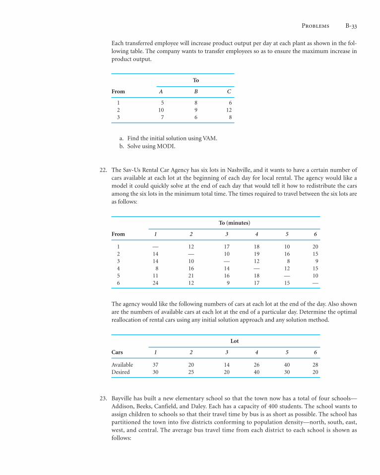
Each transferred employee will increase product output per day at each plant as shown in the fol-lowing table. The company wants to transfer employees so as to ensure the maximum increase inproduct output.

To

From A B C

1 5 8 62 10 9 123 7 6 8

a. Find the initial solution using VAM.b. Solve using MODI.

22. The Sav-Us Rental Car Agency has six lots in Nashville, and it wants to have a certain number ofcars available at each lot at the beginning of each day for local rental. The agency would like amodel it could quickly solve at the end of each day that would tell it how to redistribute the carsamong the six lots in the minimum total time. The times required to travel between the six lots areas follows:

To (minutes)

From 1 2 3 4 5 6

1 — 12 17 18 10 202 14 — 10 19 16 153 14 10 — 12 8 94 8 16 14 — 12 155 11 21 16 18 — 106 24 12 9 17 15 —

The agency would like the following numbers of cars at each lot at the end of the day. Also shownare the numbers of available cars at each lot at the end of a particular day. Determine the optimalreallocation of rental cars using any initial solution approach and any solution method.

Lot

Cars 1 2 3 4 5 6

Available 37 20 14 26 40 28Desired 30 25 20 40 30 20

23. Bayville has built a new elementary school so that the town now has a total of four schools—Addison, Beeks, Canfield, and Daley. Each has a capacity of 400 students. The school wants toassign children to schools so that their travel time by bus is as short as possible. The school haspartitioned the town into five districts conforming to population density—north, south, east,west, and central. The average bus travel time from each district to each school is shown asfollows:



Travel Time (min.)Student

District Addison Beeks Canfield Daley Population

North 12 23 35 17 250South 26 15 21 27 340East 18 20 22 31 310West 29 24 35 10 210Central 15 10 23 16 290

Determine the number of children that should be assigned from each district to each school tominimize total student travel time.

24. In Problem 23, the school board has determined that it does not want any one school to be morecrowded than any other school. It would like to assign students from each district to each school sothat enrollments are evenly balanced among the four schools. However, the school board is con-cerned that this might significantly increase travel time. Determine the number of students to beassigned from each district to each school so that school enrollments are evenly balanced. Does thisnew solution appear to result in a significant increase in travel time per student?

25. The Easy Time Grocery chain operates in major metropolitan areas on the eastern seaboard. Thestores have a “no-frills” approach, with low overhead and high volume. They generally buy theirstock in volume at low prices. However, in some cases they actually buy stock at stores in other areasand ship it in. They can do this because of high prices in the cities they operate in compared withcosts in other locations. One example is baby food. Easy Time purchases baby food at stores inAlbany, Binghamton, Claremont, Dover, and Edison and then trucks it to six stores in and aroundNew York City. The stores in the outlying areas know what Easy Time is up to, so they limit thenumber of cases of baby food Easy Time can purchase. The following table shows the profit EasyTime makes per case of baby food based on where the chain purchases it and at which store it’ssold, plus the available baby food per week at purchase locations and the shelf space available ateach Easy Time store per week:

Purchase Easy Time Store

Location 1 2 3 4 5 6 Supply

Albany 9 8 11 12 7 8 26Binghamton 10 10 8 6 9 7 40Claremont 8 6 6 5 7 4 20Dover 4 6 9 5 8 10 40Edison 12 10 8 9 6 7 45

Demand 25 15 30 18 27 35

Determine where Easy Time should purchase baby food and how the food should be distributedin order to maximize profit. Use any initial solution approach and any solution method.

26. Suppose that in Problem 25 Easy Time can purchase all the baby food it needs from a New YorkCity distributor at a price that will result in a profit of $9 per case at stores 1, 3, and 4, $8 per case atstores 2 and 6, and $7 per case at store 5. Should Easy Time purchase all, none, or some of its babyfood from the distributor rather than purchasing it at other stores and trucking it in?

27. In Problem 25, if Easy Time could arrange to purchase more baby food from one of the outlyinglocations, which should it be, how many additional cases could be purchased, and how muchwould this increase profit?


Problems B-35

28. The Roadnet Transport Company has expanded its shipping capacity by purchasing 90 trailertrucks from a competitor that went bankrupt. The company subsequently located 30 of the pur-chased trucks at each of its shipping warehouses in Charlotte, Memphis, and Louisville. The com-pany makes shipments from each of these warehouses to terminals in St. Louis, Atlanta, and NewYork. Each truck is capable of making one shipment per week. The terminal managers have indi-cated their capacity of extra shipments. The manager at St. Louis can accommodate 40 additionaltrucks per week, the manager at Atlanta can accommodate 60 additional trucks, and the manager atNew York can accommodate 50 additional trucks. The company makes the following profit pertruckload shipment from each warehouse to each terminal. The profits differ as a result of differ-ences in products shipped, shipping costs, and transport rates:

Terminal

Warehouse St. Louis Atlanta New York

Charlotte $1,800 $2,100 $1,600Memphis 1,000 700 900Louisville 1,400 800 2,200

Determine how many trucks to assign to each route (i.e., warehouse to terminal) in order tomaximize profit.

29. During the Gulf War, Operation Desert Storm required large amounts of military matériel andsupplies to be shipped daily from supply depots in the United States to bases in the Middle East.The critical factor in the movement of these supplies was speed. The following table shows thenumber of planeloads of supplies available each day from each of six supply depots and the num-ber of daily loads demanded at each of five bases. (Each planeload is approximately equal in ton-nage.) Also included are the transport hours per plane, including loading and fueling, actual flighttime, and unloading and refueling:

Supply Military Base

Depot A B C D E Supply

1 36 40 32 43 29 72 28 27 29 40 38 103 34 35 41 29 31 84 41 42 35 27 36 85 25 28 40 34 38 96 31 30 43 38 40 6

Demand 9 6 12 8 10

Determine the optimal daily flight schedule that will minimize total transport time.

30. PM Computer Services produces personal computers from component parts it buys on the openmarket. The company can produce a maximum of 300 personal computers per month. PM wantsto determine its production schedule for the first six months of the new year. The cost to produce apersonal computer in January will be $1,200. However, PM knows the cost of component parts willdecline each month such that the overall cost to produce a PC will be 5% less each month. The costof holding a computer in inventory is $15 per unit per month. Following is the demand for thecompany’s computers each month:



Month Demand Month Demand

January 180 April 210February 260 May 400March 340 June 320

Determine a production schedule for PM that will minimize total cost.

31. In Problem 30, suppose the demand for personal computers increased each month as follows:

Month Demand

January 410February 320March 500April 620May 430June 380

In addition to the regular production capacity of 300 units per month, PM Computer Services canalso produce an additional 200 computers per month using overtime. Overtime production adds20% to the cost of a personal computer.

Determine a production schedule for PM that will minimize total cost.

32. National Foods Company has five plants where it processes and packages fruits and vegetables.It has suppliers in six cities in California, Texas, Alabama, and Florida. The company hasowned and operated its own trucking system in the past for transporting fruits and vegetablesfrom its suppliers to its plants. However, it is now considering outsourcing all its shipping to out-side trucking firms and getting rid of its own trucks. It currently spends $245,000 per month tooperate its own trucking system. It has determined monthly shipping costs (in $1,000s per ton)using outside shippers from each of its suppliers to each of its plants as shown in the followingtable:

Processing Plants ($1,000s per ton)

Suppliers Denver St. Paul Louisville Akron Topeka Supply (tons)

Sacramento 3.7 4.6 4.9 5.5 4.3 18Bakersfield 3.4 5.1 4.4 5.9 5.2 15San Antonio 3.3 4.1 3.7 2.9 2.6 10Montgomery 1.9 4.2 2.7 5.4 3.9 12Jacksonville 6.1 5.1 3.8 2.5 4.1 20Ocala 6.6 4.8 3.5 3.6 4.5 15

Demand (tons) 20 15 15 15 20 90

Should National Foods continue to operate its own shipping network or sell its trucks and out-source its shipping to independent trucking firms?


Problems B-37

33. In Problem 32, National Foods would like to know what the effect would be on the optimal solu-tion and the company’s decision regarding its shipping if it negotiates with its suppliers inSacramento, Jacksonville, and Ocala to increase their capacity to 25 tons per month? What wouldbe the effect of negotiating instead with its suppliers at San Antonio and Montgomery to increasetheir capacity to 25 tons each?

34. Orient Express is a global distribution company that transports its clients’ products to customers inHong Kong, Singapore, and Taipei. All the products Orient Express ships are stored at three distri-bution centers, one in Los Angeles, one in Savannah, and one in Galveston. For the coming monththe company has 450 containers of computer components available at the Los Angeles center, 600containers available at Savannah, and 350 containers available in Galveston. The company hasorders for 600 containers from Hong Kong, 500 containers from Singapore, and 500 containersfrom Taipei. The shipping costs per container from each U.S. port to each of the overseas ports areshown in the following table:

U.S. Distribution Overseas Port

Center Hong Kong Singapore Taipei

Los Angeles $300 $210 $340Savannah 490 520 610Galveston 360 320 500

The Orient Express, as the overseas broker for its U.S. customers, is responsible for unfulfilledorders, and it incurs stiff penalty costs from overseas customers if it does not meet an order. TheHong Kong customers charge a penalty cost of $800 per container for unfulfilled demand,Singapore customers charge a penalty cost of $920 per container, and Taipei customers charge$1,100 per container. Formulate and solve a transportation model to determine the shipmentsfrom each U.S. distribution center to each overseas port that will minimize shipping costs. Indicatewhat portion of the total cost is a result of penalties.

35. Binford Tools manufactures garden tools. It uses inventory, overtime, and subcontracting to absorbdemand fluctuations. Expected demand, regular and overtime production capacity, and subcon-tracting capacity are provided in the following table for the next four quarters for its basic line ofsteel garden tools:

Regular Overtime Subcontracting Quarter Demand Capacity Capacity Capacity

1 9,000 9,000 1,000 3,0002 12,000 10,000 1,500 3,0003 16,000 12,000 2,000 3,0004 19,000 12,000 2,000 3,000

The regular production cost per unit is $20, the overtime cost per unit is $25, the cost to subcon-tract a unit is $27, and the inventory carrying cost is $2 per unit. The company has 300 units ininventory at the beginning of the year.

Determine the optimal production schedule for the four quarters that will minimize totalcosts.



36. Solve the following linear programming problem:

subject to

37. A plant has four operators to be assigned to four machines. The time (minutes) required by eachworker to produce a product on each machine is shown in the following table. Determine the opti-mal assignment and compute total minimum time.

Machine

Operator A B C D

1 10 12 9 112 5 10 7 83 12 14 13 114 8 15 11 9

38. A shop has four machinists to be assigned to four machines. The hourly cost of having eachmachine operated by each machinist is as follows:

Machine

Machinist A B C D

1 $12 11 8 142 10 9 10 83 14 8 7 114 6 8 10 9

However, because he does not have enough experience, machinist 3 cannot operate machine B.a. Determine the optimal assignment and compute total minimum cost.b. Formulate this problem as a general linear programming model.

39. The Omega pharmaceutical firm has five salespersons, whom the firm wants to assign tofive sales regions. Given their various previous contacts, the salespersons are able to cover the

xij Ú 0x14 + x24 + x34 + x44 + x54 = 1x13 + x23 + x33 + x43 + x53 = 1x12 + x22 + x32 + x42 + x52 = 1

x11 + x21 + x31 + x41 + x51 = 1x51 + x52 + x53 + x54 … 1x41 + x42 + x43 + x44 … 1x31 + x32 + x33 + x34 … 1x21 + x22 + x23 + x24 … 1x11 + x12 + x13 + x14 … 1

+ 27x43 + 29x44 + 30x51 + 26x52 + 18x53 + 24x54

+ 16x24 + 30x31 + 26x32 + 19x33 + 32x34 + 40x41 + 36x42

minimize Z = 18x11 + 30x12 + 20x13 + 18x14 + 25x21 + 27x22 + 22x23


Problems B-39

regions in different amounts of time. The amount of time (days) required by each salesperson tocover each city is shown in the following table. Which salesperson should be assigned to eachregion to minimize total time? Identify the optimal assignments and compute total minimumtime.

Region

Salesperson A B C D E

1 17 10 15 16 202 12 9 16 9 143 11 16 14 15 124 14 10 10 18 175 13 12 9 15 11

40. The Bunker Manufacturing firm has five employees and six machines and wants toassign the employees to the machines to minimize cost. A cost table showing the cost incurredby each employee on each machine follows. Because of union rules regarding departmentaltransfers, employee 3 cannot be assigned to machine E and employee 4 cannot be assignedto machine B. Solve this problem, indicate the optimal assignment, and compute total mini-mum cost.

Machine

Employee A B C D E F

1 $12 $ 7 $20 $14 $ 8 $102 10 14 13 20 9 113 5 3 6 9 7 104 9 11 7 16 9 105 10 6 14 8 10 12

41. Given the following cost table for an assignment problem, determine the optimal assignmentand compute total minimum cost. Identify all alternative solutions if there are multiple optimalsolutions.

Machine

Operator A B C D

1 $10 $2 $ 8 $ 62 9 5 11 93 12 7 14 144 3 1 4 2

42. An electronics firm produces electronic components, which it supplies to various electrical manu-facturers. Quality control records indicate that different employees produce different numbers ofdefective items. The average number of defects produced by each employee for each of six components



is given in the following table. Determine the optimal assignment that will minimize the total aver-age number of defects produced by the firm per month.

Component

Employee A B C D E F

1 30 24 16 26 30 222 22 28 14 30 20 133 18 16 25 14 12 224 14 22 18 23 21 305 25 18 14 16 16 286 32 14 10 14 18 20

43. A dispatcher for the Citywide Taxi Company has six taxicabs at different locations and five cus-tomers who have called for service. The mileage from each taxi’s present location to each customeris shown in the following table. Determine the optimal assignment(s) that will minimize the totalmileage traveled.

Customer

Cab 1 2 3 4 5

A 7 2 4 10 7B 5 1 5 6 6C 8 7 6 5 5D 2 5 2 4 5E 3 3 5 8 4F 6 2 4 3 4

44. The Southeastern Conference has nine basketball officials who must be assigned to three confer-ence games, three to each game. The conference office wants to assign the officials so that the totaldistance they travel will be minimized. The distance (in miles) each official would travel to eachgame is given in the following table:

Game

Official Athens Columbia Nashville

1 165 90 1302 75 210 3203 180 170 1404 220 80 605 410 140 806 150 170 1907 170 110 1508 105 125 1609 240 200 155


Problems B-41

a. Should this problem be solved by the transportation method or by the assignment method?Explain.

b. Determine the optimal assignment(s) that will minimize the total distance traveled by theofficials.

45. In Problem 44, officials 2 and 8 had a recent confrontation with one of the coaches in the game inAthens. They were forced to eject the coach after several technical fouls. The conference officedecided that it would not be a good idea to have these two officials work the Athens game so soonafter this confrontation, so they decided that officials 2 and 8 will not be assigned to the Athensgame. How will this affect the optimal solution to this problem?

46. State University has planned six special catered events for the November Saturday of its homecom-ing football game. The events include an alumni brunch, a parents’ brunch, a booster club lun-cheon, a postgame party for season ticket holders, a lettermen’s dinner, and a fund-raising dinnerfor major contributors. The university wants to use local catering firms as well as the universitycatering service to cater these events and it has asked the caterers to bid on each event. The bids (in$1,000s) based on menu guidelines for the events prepared by the university are shown in the fol-lowing table:

Event

Alumni Parents’ Booster Postgame Lettermen’s Contributor’s Caterer Brunch Brunch Club Lunch Party Dinner Dinner

Al’s $12.6 $10.3 $14.0 $19.5 $25.0 $30.0Bon Apetít 14.5 13.0 16.5 17.0 22.5 32.0Custom 13.0 14.0 17.6 21.5 23.0 35.0Divine 11.5 12.6 13.0 18.7 26.2 33.5Epicurean 10.8 11.9 12.9 17.5 21.9 28.5Fouchés 13.5 13.5 15.5 22.3 24.5 36.0University 12.5 14.3 16.0 22.0 26.7 34.0

The Bon Apetít, Custom, and University caterers can handle two events, whereas the other fourcaterers can handle only one. The university is confident all the caterers will do a high-quality job,so it wants to select the caterers for the events that will result in the lowest total cost.

Determine the optimal selection of caterers that will minimize total cost.

47. A university department head has five instructors to be assigned to four different courses. All theinstructors have taught the courses in the past and have been evaluated by the students. The ratingfor each instructor for each course is given in the following table (a perfect score is 100). Thedepartment head wants to know the optimal assignment of instructors to courses that will maxi-mize the overall average evaluation. The instructor who is not assigned to teach a course will beassigned to grade exams. Solve this problem using the assignment method.

Course

Instructor A B C D

1 80 75 90 852 95 90 90 973 85 95 88 914 93 91 80 845 91 92 93 88



48. The coach of the women’s swim team at State University is preparing for the conference swim meetand must choose the four swimmers she will assign to the 800-meter medley relay team. Themedley relay consists of four strokes—the backstroke, breaststroke, butterfly, and freestyle. Thecoach has computed the average times (in minutes) each of her top six swimmers has achieved ineach of the four strokes for 200 meters in previous swim meets during the season as follows:

Stroke (min)

Swimmer Backstroke Breaststroke Butterfly Freestyle

Annie 2.56 3.07 2.90 2.26Beth 2.63 3.01 3.12 2.35Carla 2.71 2.95 2.96 2.29Debbie 2.60 2.87 3.08 2.41Erin 2.68 2.97 3.16 2.25Fay 2.75 3.10 2.93 2.38

Determine the medley relay team and its total expected relay time for the coach.

49. Biggio’s Department Store has six employees available to assign to four departments in the store—home furnishings, china, appliances, and jewelry. Most of the six employees have worked in each ofthe four departments on several occasions in the past and have demonstrated that they performbetter in some departments than in others. The average daily sales for each of the six employees ineach of the four departments is shown in the following table.

Department Sales ($)

Home Employee Furnishings China Appliances Jewelry

1 340 160 610 2902 560 370 520 4503 270 — 350 4204 360 220 630 1505 450 190 570 3106 280 320 490 360

Employee 3 has not worked in the china department before, so the manager does not want to assignthis employee to china.

Determine which employee to assign to each department and indicate the total expected dailysales.

50. The Vanguard Publishing Company has eight college students it hires as salespeople to sell encyclo-pedias during the summer. The company desires to allocate them to three sales territories. Territory1 requires three salespeople, and territories 2 and 3 require two salespeople each. It is estimated thateach salesperson will be able to generate the amounts of dollar sales per day in each of the three ter-ritories as given in the following table. The company desires to allocate the salespeople to the threeterritories so that sales will be maximized. Solve this problem using any method to determine theinitial solution and any solution method. Compute the maximum total sales per day.


Problems B-43

Territory

Salesperson 1 2 3

A $110 $150 $130B 90 120 80C 205 160 175D 125 100 115E 140 105 150F 100 140 120G 180 210 160H 110 120 90

51. Carolina Airlines, a small commuter airline in North Carolina, has six flight attendants whom itwants to assign to six monthly flight schedules in a way that will minimize the number of nightsthey will be away from their homes. The numbers of nights each attendant must be away fromhome with each schedule are given in the following table. Identify the optimal assignments that willminimize the total number of nights the attendants will be away from home.

Schedule

Attendant A B C D E F

1 7 4 5 10 5 72 4 5 4 12 7 53 9 9 10 7 10 74 11 6 7 5 9 95 5 8 5 10 7 56 10 12 10 9 9 9

52. The football coaching staff at Tech focuses its recruiting on several key states, including Georgia,Florida, Virginia, Pennsylvania, New York, and New Jersey. The staff includes seven assistantcoaches, two of whom are responsible for Florida, a high school talent–rich state, whereas onecoach is assigned to each of the other five states. The staff has been together for a long time and atone time or another all the coaches have recruited all of the states. The head coach has accumulatedsome data on the past success rate (i.e., percentage of targeted recruits signed) for each coach ineach state as shown in the following table:

State

Coach GA FL VA PA NY NJ

Allen 62 56 65 71 55 63Bush 65 70 63 81 75 72Crumb 46 53 62 55 64 50Doyle 58 66 70 67 71 49Evans 77 73 69 80 80 74Fouch 68 73 72 80 78 57Goins 72 60 74 72 62 61

Determine the optimal assignment of coaches to recruiting regions that will maximize the over-all success rate and indicate the average percentage success rate for the staff with this assignment.


Module B Transportation and Assignment Solution...

Documents

Transcript of Module B Transportation and Assignment Solution...