MODERN SPECTROSCOPY - nsc.ru · 6.1.4 Vibration–rotation spectroscopy 147 6.1.4.1 Infrared...
483
Transcript of MODERN SPECTROSCOPY - nsc.ru · 6.1.4 Vibration–rotation spectroscopy 147 6.1.4.1 Infrared...


MODERNSPECTROSCOPY
Fourth Edition


MODERNSPECTROSCOPY
Fourth Edition
J. Michael HollasUniversity of Reading

Copyright # 1987, 1992, 1996, 2004 by John Wiley & Sons Ltd, The Atrium, Southern Gate,Chichester, West Sussex PO19 8SQ, England
Telephone (þ44) 1243 779777
Email (for orders and customer service enquiries): [email protected] our Home Page on www.wileyeurope.com or www.wiley.com
All rights reserved. No part of this publication may be reproduced, stored in a retrievalsystem or transmitted in any form or by any means, electronic, mechanical, photocopying,recording, scanning or otherwise, except under the terms of the Copyright, Designs andPatents Act 1988 or under the terms of a licence issued by the Copyright Licensing AgencyLtd, 90 Tottenham Court Road, London W1T 4LP, UK, without the permission in writing ofthe Publisher. Requests to the Publisher should be addressed to the Permissions Department,John Wiley & Sons Ltd, The Atrium, Southern Gate, Chichester, West Sussex PO19 8SQ,England, or emailed to [email protected], or faxed to (þ44) 1243 770620.
This publication is designed to provide accurate and authoritative information in regard tothe subject matter covered. It is sold on the understanding that the Publisher is not engagedin rendering professional services. If professional advice or other expert assistance isrequired, the services of a competent professional should be sought.
Other Wiley Editorial Offices
John Wiley & Sons, Inc., 111 River Street, Hoboken, NJ 07030, USA
Jossey-Bass, 989 Market Street, San Francisco, CA 94103-1741, USA
Wiley-VCH Verlag GmbH, Boschstr. 12, D-69469 Weinheim, Germany
John Wiley & Sons Australia Ltd, 33 Park Road, Milton, Queensland 4064, Australia
John Wiley & Sons (Asia) Pte Ltd, 2 Clementi Loop #02-01, Jin Xing Distripark, Singapore129809
John Wiley & Sons Canada Ltd, 22 Worcester Road, Etobicoke, Ontario, Canada M9W 1L1
Wiley also publishes its books in a variety of electronic formats. Some content that appearsin print may not be available in electronic books.
British Library Cataloguing in Publication Data
A catalogue record for this book is available from the British Library
ISBN 0 470 84415 9 (cloth)ISBN 0 470 84416 7 (paper)
Typeset in 10.5=12.5pt Times by Techset Composition Limited, Salisbury, UKPrinted and bound in Great Britain by Anthony Rowe Ltd, Chippenham, WiltsThis book is printed on acid-free paper responsibly manufactured from sustainable forestryin which at least two trees are planted for each one used for paper production.
Contents
Preface to first edition xiii
Preface to second edition xv
Preface to third edition xvii
Preface to fourth edition xix
Units, dimensions and conventions xxi
Fundamental constants xxiii
Useful conversion factors xxv
1 Some important results in quantum mechanics 1
1.1 Spectroscopy and quantum mechanics 1
1.2 The evolution of quantum theory 2
1.3 The Schrodinger equation and some of its solutions 8
1.3.1 The Schrodinger equation 91.3.2 The hydrogen atom 111.3.3 Electron spin and nuclear spin angular momentum 17
1.3.4 The Born–Oppenheimer approximation 191.3.5 The rigid rotor 211.3.6 The harmonic oscillator 23
Exercises 25
Bibliography 26
2 Electromagnetic radiation and its interaction with atomsand molecules 27
2.1 Electromagnetic radiation 27
2.2 Absorption and emission of radiation 27
2.3 Line width 34
2.3.1 Natural line broadening 342.3.2 Doppler broadening 352.3.3 Pressure broadening 36
2.3.4 Power, or saturation, broadening 362.3.5 Removal of line broadening 37
2.3.5.1 Effusive atomic or molecular beams 372.3.5.2 Lamb dip spectroscopy 37
v
Exercises 38
Bibliography 39
3 General features of experimental methods 41
3.1 The electromagnetic spectrum 41
3.2 General components of an absorption experiment 42
3.3 Dispersing elements 43
3.3.1 Prisms 433.3.2 Diffraction gratings 45
3.3.3 Fourier transformation and interferometers 483.3.3.1 Radiofrequency radiation 493.3.3.2 Infrared, visible and ultraviolet radiation 55
3.4 Components of absorption experiments in various regions of the spectrum 59
3.4.1 Microwave and millimetre wave 593.4.2 Far-infrared 613.4.3 Near-infrared and mid-infrared 623.4.4 Visible and near-ultraviolet 62
3.4.5 Vacuum- or far-ultraviolet 63
3.5 Other experimental techniques 64
3.5.1 Attenuated total reflectance spectroscopy and
reflection–absorption infrared spectroscopy 64
3.5.2 Atomic absorption spectroscopy 643.5.3 Inductively coupled plasma atomic emission spectroscopy 663.5.4 Flash photolysis 67
3.6 Typical recording spectrophotometers for the near-infrared, mid-infrared,
visible and near-ultraviolet regions 68
Exercise 70
Bibliography 70
4 Molecular symmetry 73
4.1 Elements of symmetry 73
4.1.1 n-Fold axis of symmetry, Cn 744.1.2 Plane of symmetry, s 754.1.3 Centre of inversion, i 76
4.1.4 n-Fold rotation–reflection axis of symmetry, Sn 764.1.5 The identity element of symmetry, I (or E) 774.1.6 Generation of elements 77
4.1.7 Symmetry conditions for molecular chirality 78
4.2 Point groups 81
4.2.1 Cn point groups 824.2.2 Sn point groups 83
4.2.3 Cnv point groups 834.2.4 Dn point groups 834.2.5 Cnh point groups 844.2.6 Dnd point groups 84
4.2.7 Dnh point groups 84
vi CONTENTS
4.2.8 Td point group 854.2.9 Oh point group 85
4.2.10 Kh point group 864.2.11 Ih point group 864.2.12 Other point groups 87
4.3 Point group character tables 87
4.3.1 C2v character table 874.3.2 C3v character table 924.3.3 C1v character table 964.3.4 Ih character table 97
4.4 Symmetry and dipole moments 97
Exercises 102
Bibliography 102
5 Rotational spectroscopy 103
5.1 Linear, symmetric rotor, spherical rotor and asymmetric rotor molecules 103
5.2 Rotational infrared, millimetre wave and microwave spectra 105
5.2.1 Diatomic and linear polyatomic molecules 1055.2.1.1 Transition frequencies or wavenumbers 1055.2.1.2 Intensities 1105.2.1.3 Centrifugal distortion 1115.2.1.4 Diatomic molecules in excited vibrational states 112
5.2.2 Symmetric rotor molecules 1135.2.3 Stark effect in diatomic, linear and symmetric rotor molecules 115
5.2.4 Asymmetric rotor molecules 1165.2.5 Spherical rotor molecules 1175.2.6 Interstellar molecules detected by their radiofrequency, microwave
or millimetre wave spectra 119
5.3 Rotational Raman spectroscopy 122
5.3.1 Experimental methods 1225.3.2 Theory of rotational Raman scattering 124
5.3.3 Rotational Raman spectra of diatomic and linear polyatomic
molecules 1265.3.4 Nuclear spin statistical weights 128
5.3.5 Rotational Raman spectra of symmetric and asymmetric rotor
molecules 131
5.4 Structure determination from rotational constants 131
Exercises 134
Bibliography 135
6 Vibrational spectroscopy 137
6.1 Diatomic molecules 137
6.1.1 Infrared spectra 138
6.1.2 Raman spectra 1406.1.3 Anharmonicity 142
6.1.3.1 Electrical anharmonicity 1426.1.3.2 Mechanical anharmonicity 142
CONTENTS vii
6.1.4 Vibration–rotation spectroscopy 1476.1.4.1 Infrared spectra 1476.1.4.2 Raman spectra 151
6.2 Polyatomic molecules 154
6.2.1 Group vibrations 1546.2.2 Number of normal vibrations of each symmetry species 162
6.2.2.1 Non-degenerate vibrations 1636.2.2.2 Degenerate vibrations 165
6.2.3 Vibrational selection rules 1666.2.3.1 Infrared spectra 1666.2.3.2 Raman spectra 172
6.2.4 Vibration–rotation spectroscopy 1736.2.4.1 Infrared spectra of linear molecules 1746.2.4.2 Infrared spectra of symmetric rotors 1786.2.4.3 Infrared spectra of spherical rotors 1806.2.4.4 Infrared spectra of asymmetric rotors 181
6.2.5 Anharmonicity 1846.2.5.1 Potential energy surfaces 1846.2.5.2 Vibrational term values 1866.2.5.3 Local mode treatment of vibrations 1876.2.5.4 Vibrational potential functions with more than one minimum 1886.2.5.4(a) Inversion vibrations 1896.2.5.4(b) Ring-puckering vibrations 1916.2.5.4(c) Torsional vibrations 192
Exercises 195
Bibliography 196
7 Electronic spectroscopy 199
7.1 Atomic spectroscopy 199
7.1.1 The periodic table 1997.1.2 Vector representation of momenta and vector coupling approximations 201
7.1.2.1 Angular momenta and magnetic moments 2017.1.2.2 Coupling of angular momenta 2057.1.2.3 Russell–Saunders coupling approximation 2067.1.2.3(a) Non-equivalent electrons 2067.1.2.3(b) Equivalent electrons 210
7.1.3 Spectra of alkali metal atoms 2137.1.4 Spectrum of the hydrogen atom 216
7.1.5 Spectra of helium and the alkaline earth metal atoms 2197.1.6 Spectra of other polyelectronic atoms 222
7.2 Electronic spectroscopy of diatomic molecules 225
7.2.1 Molecular orbitals 2257.2.1.1 Homonuclear diatomic molecules 2257.2.1.2 Heteronuclear diatomic molecules 232
7.2.2 Classification of electronic states 2337.2.3 Electronic selection rules 236
7.2.4 Derivation of states arising from configurations 2377.2.5 Vibrational coarse structure 240
7.2.5.1 Potential energy curves in excited electronic states 2407.2.5.2 Progressions and sequences 242
viii CONTENTS
7.2.5.3 The Franck–Condon principle 2467.2.5.4 Deslandres tables 2507.2.5.5 Dissociation energies 2507.2.5.6 Repulsive states and continuous spectra 253
7.2.6 Rotational fine structure 2547.2.6.1 1S7 1S electronic and vibronic transitions 2547.2.6.2 1P7 1S electronic and vibronic transitions 257
7.3 Electronic spectroscopy of polyatomic molecules 260
7.3.1 Molecular orbitals and electronic states 2607.3.1.1 AH2 molecules 2617.3.1.1(a) ffHAH¼ 180� 2617.3.1.1(b) ffHAH¼ 90� 263
7.3.1.2 Formaldehyde (H2CO) 2657.3.1.3 Benzene 2677.3.1.4 Crystal field and ligand field molecular orbitals 2707.3.1.4(a) Crystal field theory 2717.3.1.4(b) Ligand field theory 2737.3.1.4(c) Electronic transitions 275
7.3.2 Electronic and vibronic selection rules 2757.3.3 Chromophores 278
7.3.4 Vibrational coarse structure 2787.3.4.1 Sequences 2787.3.4.2 Progressions 2797.3.4.2(a) Totally symmetric vibrations 2797.3.4.2(b) Non-totally symmetric vibrations 279
7.3.5 Rotational fine structure 2837.3.6 Diffuse spectra 284
Exercises 287
Bibliography 288
8 Photoelectron and related spectroscopies 289
8.1 Photoelectron spectroscopy 289
8.1.1 Experimental methods 2918.1.1.1 Sources of monochromatic ionizing radiation 2918.1.1.2 Electron velocity analysers 2948.1.1.3 Electron detectors 2948.1.1.4 Resolution 294
8.1.2 Ionization processes and Koopmans’ theorem 295
8.1.3 Photoelectron spectra and their interpretation 2978.1.3.1 Ultraviolet photoelectron spectra of atoms 2978.1.3.2 Ultraviolet photoelectron spectra of molecules 2988.1.3.2(a) Hydrogen 2988.1.3.2(b) Nitrogen 3008.1.3.2(c) Hydrogen bromide 3028.1.3.2(d) Water 3058.1.3.2(e) Benzene 305
8.1.3.3 X-ray photoelectron spectra of gases 3078.1.3.4 X-ray photoelectron spectra of solids 313
8.2 Auger electron and X-ray fluorescence spectroscopy 315
8.2.1 Auger electron spectroscopy 3178.2.1.1 Experimental method 317
CONTENTS ix
8.2.1.2 Processes in Auger electron ejection 3188.2.1.3 Examples of Auger electron spectra 319
8.2.2 X-ray fluorescence spectroscopy 3228.2.2.1 Experimental method 3228.2.2.2 Processes in X-ray fluorescence 3248.2.2.3 Examples of X-ray fluorescence spectra 325
8.3 Extended X-ray absorption fine structure 327
Exercises 334
Bibliography 335
9 Lasers and laser spectroscopy 337
9.1 General discussion of lasers 337
9.1.1 General features and properties 3379.1.2 Methods of obtaining population inversion 3409.1.3 Laser cavity modes 341
9.1.4 Q-switching 3429.1.5 Mode locking 3449.1.6 Harmonic generation 345
9.2 Examples of lasers 346
9.2.1 The ruby and alexandrite lasers 3469.2.2 The titanium–sapphire laser 3489.2.3 The neodymium–YAG laser 349
9.2.4 The diode or semiconductor laser 3509.2.5 The helium–neon laser 3529.2.6 The argon ion and krypton ion lasers 3549.2.7 The nitrogen (N2) laser 355
9.2.8 The excimer and exciplex lasers 3569.2.9 The carbon dioxide laser 3589.2.10 The dye lasers 359
9.2.11 Laser materials in general 362
9.3 Uses of lasers in spectroscopy 362
9.3.1 Hyper Raman spectroscopy 3639.3.2 Stimulated Raman spectroscopy 365
9.3.3 Coherent anti-Stokes Raman scattering spectroscopy 3679.3.4 Laser Stark (or laser electron resonance) spectroscopy 3689.3.5 Two-photon and multiphoton absorption 371
9.3.6 Multiphoton dissociation and laser separation of isotopes 3749.3.7 Single vibronic level, or dispersed, fluorescence 3779.3.8 Light detection and ranging (LIDAR) 379
9.3.9 Cavity ring-down spectroscopy 3829.3.10 Femtosecond spectroscopy 3879.3.11 Spectroscopy of molecules in supersonic jets 393
9.3.11.1 Properties of a supersonic jet 3939.3.11.2 Fluorescence excitation spectroscopy 3969.3.11.3 Single vibronic level, or dispersed, fluorescence
spectroscopy 4009.3.11.4 Zero kinetic energy photoelectron spectroscopy 402
Exercises 404
Bibliography 405
x CONTENTS

Appendix
A Character tables 407
B Symmetry species of vibrations 423
Index of Atoms and Molecules 429
Subject Index 439
CONTENTS xi

Preface to first edition
Modern Spectroscopy has been written to fulfil a need for an up-to-date text on spectroscopy.
It is aimed primarily at a typical undergraduate audience in chemistry, chemical physics, or
physics in the United Kingdom and at undergraduate and graduate student audiences
elsewhere.
Spectroscopy covers a very wide area which has been widened further since the mid-
1960s by the development of lasers and such techniques as photoelectron spectroscopy and
other closely related spectroscopies. The importance of spectroscopy in the physical and
chemical processes going on in planets, stars, comets and the interstellar medium has
continued to grow as a result of the use of satellites and the building of radiotelescopes for
the microwave and millimetre wave regions.
In planning a book of this type I encountered three major problems. The first is that of
covering the analytical as well as the more fundamental aspects of the subject. The
importance of the applications of spectroscopy to analytical chemistry cannot be overstated,
but the use of many of the available techniques does not necessarily require a detailed
understanding of the processes involved. I have tried to refer to experimental methods and
analytical applications where relevant.
The second problem relates to the inclusion, or otherwise, of molecular symmetry
arguments. There is no avoiding the fact that an understanding of molecular symmetry
presents a hurdle (although I think it is a low one) which must be surmounted if selection
rules in vibrational and electronic spectroscopy of polyatomic molecules are to be
understood. This book surmounts the hurdle in Chapter 4, which is devoted to molecular
symmetry but which treats the subject in a non-mathematical way. For those lecturers and
students who wish to leave out this chapter much of the subsequent material can be
understood but, in some areas, in a less satisfying way.
The third problem also concerns the choice of whether to leave out certain material. In a
book of this size it is not possible to cover all branches of spectroscopy. Such decisions are
difficult ones but I have chosen not to include spin resonance spectroscopy (NMR and ESR),
nuclear quadrupole resonance spectroscopy (NQR), and Mossbauer spectroscopy. The
exclusion of these areas, which have been well covered in other texts, has been caused, I
suppose, by the inclusion, in Chapter 8, of photoelectron spectroscopy (ultraviolet and X-
ray), Auger electron spectroscopy, and extended X-ray absorption fine structure, including
applications to studies of solid surfaces, and, in Chapter 9, the theory and some examples of
lasers and some of their uses in spectroscopy. Most of the material in these two chapters will
not be found in comparable texts but is of very great importance in spectroscopy today.
xiii
My understanding of spectroscopy owes much to having been fortunate in working in and
discussing the subject with Professor I. M. Mills, Dr A. G. Robiette, Professor J. A. Pople,
Professor D. H. Whiffen, Dr J. K. G. Watson, Dr G. Herzberg, Dr A. E. Douglas, Dr D. A.
Ramsay, Professor D. P. Craig, Professor J. H. Callomon, and Professor G. W. King (in more
or less reverse historical order), and I am grateful to all of them.
When my previous book High Resolution Spectroscopy was published by Butterworths in
1982 I had it in mind to make some of the subject matter contained in it more accessible to
students at a later date. This is what I have tried to do in Modern Spectroscopy and I would
like to express my appreciation to Butterworths for allowing me to use some textual material
and, particularly, many of the figures from High Resolution Spectroscopy. New figures were
very competently drawn by Mr M. R. Barton.
Although I have not included High Resolution Spectroscopy in the bibliography of any of
the chapters it is recommended as further reading on all topics.
Mr A. R. Bacon helped greatly with the page proof reading and I would like to thank him
very much for his careful work. Finally, I would like to express my sincere thanks to Mrs A.
Gillett for making such a very good job of typing the manuscript.
J. Michael Hollas
xiv PREFACE TO FIRST EDITION
Preface to second edition
A new edition of any book presents an opportunity which an author welcomes for several
reasons. It is a chance to respond to constructive criticisms of the previous edition which he
thinks are valid. New material can be introduced which may be useful to teachers and
students in the light of the way the subject, and the teaching of the subject, has developed in
the intervening years. Last, and certainly not least, there is an opportunity to correct any
errors which had escaped the author’s notice.
Fourier transformation techniques in spectroscopy are now quite common—the latest to
arrive on the scene is Fourier transform Raman spectroscopy. In Chapter 3 I have expanded
considerably the discussion of these techniques and included Fourier transform Raman
spectroscopy for the first time.
In teaching students about Fourier transform techniques I find it easier to introduce the
subject by using radiofrequency radiation, for which the variations of the signal with time
can be readily detected—as happens in an ordinary radio. Fourier transformation of the
radiofrequency signal, which the radio itself carries out, is quite easy to visualize without
going deeply into the mathematics. The use of a Michelson interferometer in the infrared,
visible or ultraviolet regions is necessary because of the inability of a detector to respond to
these higher frequencies, but I think the way in which it gets over this problem is rather
subtle. In this second edition I have discussed Fourier transformation, relating first to
radiofrequency and then to higher frequency radiation.
In the first edition of Modern Spectroscopy I tried to go some way towards bridging the
gulf that often seems to exist between high resolution spectroscopy and low resolution, often
analytical, spectroscopy. In this edition I have gone further by including X-ray fluorescence
spectroscopy and inductively coupled plasma atomic emission spectroscopy, both of which
are used almost entirely for analytical purposes. I think it is important that the user
understand the processes going on in any analytical spectroscopic technique that he or she
might be using.
In Chapter 4, on molecular symmetry, I have added two new sections. One of these
concerns the relationship between symmetry and chirality, which is of great importance in
synthetic organic chemistry. The other relates to the connection between the symmetry of a
molecule and whether it has a permanent dipole moment.
In the chapter on vibrational spectroscopy (Chapter 6) I have expanded the discussions of
inversion, ring-puckering and torsional vibrations, including some model potential
functions. These types of vibration are very important in the determination of molecular
structure.
xv
The development of lasers has continued in the past few years and I have included
discussions of two more in this edition. These are the alexandrite and titanium–sapphire
lasers. Both are solid state and, unusually, tunable over quite wide wavelength ranges. The
titanium–sapphire laser is probably the most promising for general use because of its wider
range of tunability and the fact that it can be operated in a CW or pulsed mode.
Laser spectroscopy is such a wide subject, with many ingenious experiments using one or
two CW or pulsed lasers to study atomic or molecular structure or dynamics, that it is
difficult to do justice to it at the level at which Modern Spectroscopy is aimed. In this edition
I have expanded the section on supersonic jet spectroscopy, which is an extremely important
and wide-ranging field.
I would like to thank Professor I. M. Mills for the material he provided for Figure 3.14(b)
and Figure 3.16 and Dr P. Hollins for help in the production of Figures 3.7(a), 3.8(a), 3.9(a)
and 3.10(a). The spectrum in Figure 9.36 will be published in a paper by Dr J. M. Hollas and
Dr P. F. Taday.
J. Michael Hollas
xvi PREFACE TO SECOND EDITION
Preface to third edition
One of the more obvious changes from the second edition which Modern Spectroscopy has
undergone concerns the page size. The consequent new format of the pages is much less
crowded and more user friendly.
Much of the additional material is taken up by what I have called ‘Worked examples’.
These are sample problems, which are mostly calculations, with answers given in some
detail. There are seventeen of them scattered throughout the book in positions in the text
appropriate to the theory which is required. I believe that these will be very useful in
demonstrating to the reader how problems should be tackled. In the calculations, I have paid
particular attention to the number of significant figures retained and to the correct use of
units. I have stressed the importance of putting in the units in a calculation. In a typical
example, for the calculation of the rotational constant B for a diatomic molecule from the
equation
B ¼ h
8p2cmr2where m ¼ m1m2
m1 þ m2
it is an invaluable help in getting the correct answer to check the units with which m has been
calculated and then to put the units of all quantities involved into the equation for B.
Molecules with icosahedral symmetry are not new but the discovery of the newest of
them, C60 or buckminsterfullerene, has had such a profound effect on chemistry in recent
years that I thought it useful to include a discussion of the icosahedral point group to which
C60 belongs.
Use of the supersonic jet in many branches of spectroscopy continues to increase. One
technique which has made a considerable impact in recent years is that of zero kinetic
energy photoelectron (ZEKE-PE) spectroscopy. Because of its increasing importance and
the fact that it relates closely to ultraviolet photoelectron spectroscopy (UPS), which is
described at length in earlier editions, I have included the new technique in Chapter 9.
Charge coupled device (CCD) detectors are being used increasingly in the visible and
ultraviolet regions. At present these are very expensive but I have anticipated their increasing
importance by including a brief description in Chapter 3.
There are some quite simple symmetry rules for dividing the total number of vibrations of
a polyatomic molecule into symmetry classes. The principles behind these, and the rules
themselves, have been added to Chapter 4.
xvii

I would like to thank Professor B. van der Veken for the improved FTIR spectrum in
Figure 6.8.
J. Michael Hollas
xviii PREFACE TO THIRD EDITION
Preface to fourth edition
Spectroscopy occupies a very special position in chemistry, physics and in science in
general. It is capable of providing accurate answers to some of the most searching questions,
particularly those concerning atomic and molecular structure. For small molecules, it can
provide accurate values of bond lengths and bond angles. For larger molecules, details of
conformation can be obtained. Is a molecule planar? If it is non-planar, what is the energy
barrier to planarity? Does a methyl group attached to a benzene ring take up the eclipsed or
staggered position? Is a cis or trans conformation more stable? Spectroscopy provides
techniques that are vital in chemical analysis and in the investigation of the composition of
planets, comets, stars and the interstellar medium.
At the research level, spectroscopy continues to flourish and is continually developing
with occasional quantum leaps. For example, such a leap resulted from the development of
lasers. Not all leaps provide suitable material for inclusion in an undergraduate text such as
this. However, even in the relatively short period of seven years since the third edition, there
have been either new developments or consolidation of rather less recent ones, which are not
only of the greatest importance but which can (I hope!) be communicated at this level.
New to the fourth edition are the topics of laser detection and ranging (LIDAR), cavity
ring-down spectroscopy, femtosecond lasers and femtosecond spectroscopy, and the use of
laser-induced fluorescence excitation for structural investigations of much larger molecules
than had been possible previously. This latter technique takes advantage of two experimental
quantum leaps: the development of very high resolution lasers in the visible and ultraviolet
regions and of the supersonic molecular beam.
Since the first edition in 1987 there has been some loss of clarity in those figures that have
been used in subsequent editions. The presentation of figures in this new edition has been
improved and small changes, additions and corrections have been made to the text. I am very
grateful to Robert Hambrook (John Wiley) and Rachel Catt who have contributed greatly to
these improvements. The fundamental constants have been updated. Apart from the speed of
light, which is defined exactly, many of these are continually being determined with greater
accuracy.
New books on spectroscopy continue to be published while some of the older ones remain
classics. The bibliography has been brought up to date to include some of the new
publications, or new editions of older ones.
I have not included in the bibliography my own books on spectroscopy. High Resolution
Spectroscopy, second edition (John Wiley, 1998) follows the general format of Modern
Spectroscopy but takes the subject to the research level. Basic Atomic and Molecular
xix

Spectroscopy (Royal Society of Chemistry, 2002) approaches the subject at a simpler level
than Modern Spectroscopy, being fairly non-mathematical and including many worked
problems. Neither book is included in the bibliography but each is recommended as
additional reading, depending on the level required.
I am particularly grateful to Professor Ben van der Veken (University of Antwerp) who
has obtained new spectra, with an infrared interferometer, which are shown in Figures 6.8,
6.27, 6.28 and 6.34, and to Dr Andrew Orr-Ewing (University of Bristol), who provided
original copies of the cavity ring-down spectra in Figures 9.38 and 9.39.
J. Michael Hollas
xx PREFACE TO FOURTH EDITION
Units, dimensions and conventions
Throughout the book I have adhered to the SI system of units, with a few exceptions. The
angstrom (A) unit, where 1 A¼ 10710 m, seems to be persisting generally when quoting
bond lengths, which are of the order of 1 A. I have continued this usage but, when quoting
wavelengths in the visible and near-ultraviolet regions, I have used the nanometre, where
1 nm¼ 10 A. The angstrom is still used sometimes in this context but it seems just as
convenient to write, say, 352.3 nm as 3523 A.
In photoelectron and related spectroscopies, ionization energies are measured. For
many years such energies have been quoted in electron volts, where 1 eV¼1.602 176 4626 10719 J, and I have continued to use this unit.
Pressure measurements are not often quoted in the text but the unit of Torr, where
1 Torr¼ 1 mmHg¼ 133.322 387 Pa, is a convenient practical unit and appears occasion-
ally.
Dimensions are physical quantities such as mass (M), length (L), and time (T) and
examples of units corresponding to these dimensions are the gram (g), metre (m) and second
(s). If, for example, something has a mass of 3.5 g then we write
m ¼ 3:5 g
Units, here the gram, can be treated algebraically so that, if we divide both sides by ‘g’, we
get
m=g ¼ 3:5
The right-hand side is now a pure number and, if we wish to plot mass, in grams, against,
say, volume on a graph we label the mass axis ‘m=g’so that the values marked along the axis
are pure numbers. Similarly, if we wish to tabulate a series of masses, we put ‘m=g’ at thehead of a column of what are now pure numbers. The old style of using ‘m(g)’ is now seen
to be incorrect as, algebraically, it could be interpreted only as m6 g rather than m � g,
which we require.
An issue that is still only just being resolved concerns the use of the word ‘wavenumber’.
Whereas the frequency n of electromagnetic radiation is related to the wavelength l by
n ¼ c
l
xxi
where c is the speed of light, the wavenumber ~nn is simply its reciprocal:
~nn ¼ 1
l
Since c has dimensions of LT71 and l those of L, frequency has dimensions of T71 and
often has units of s71 (or hertz). On the other hand, wavenumber has dimensions of L71 and
often has units of cm71. Therefore
n ¼ 15:3 s�1 ðor hertzÞ
is, in words, ‘the frequency is 15.3 reciprocal seconds (or second-minus-one or hertz)’, and
~nn ¼ 20:6 cm�1
is, in words, ‘the wavenumber is 20.6 reciprocal centimetres (or centimetre-minus-one)’. All
of this seems simple and straightforward but the fact is that many of us would put the second
equation, in words, as ‘the frequency is 20.6 wavenumbers’. This is quite illogical but very
common – although not, I hope, in this book.
Another illogicality is the very common use of the symbols A, B and C for rotational
constants irrespective of whether they have dimensions of frequency or wavenumber. It is
bad practice to do this, but although a few have used ~AA, ~BB and ~CC to imply dimensions of
wavenumber, this excellent idea has only rarely been put into practice and, regretfully, I go
along with a very large majority and use A, B and C whatever their dimensions.
The starting points for many conventions in spectroscopy are the paper by R. S. Mulliken
in the Journal of Chemical Physics (23, 1997, 1955) and the books of G. Herzberg. Apart
from straightforward recommendations of symbols for physical quantities, which are
generally adhered to, there are rather more contentious recommendations. These include the
labelling of cartesian axes in discussions of molecular symmetry and the numbering of
vibrations in a polyatomic molecule, which are often, but not always, used. In such cases it is
important that any author make it clear what convention is being used.
The case of vibrational numbering in, say, fluorobenzene illustrates the point that we must
be flexible when it may be helpful. Many of the vibrations of fluorobenzene strongly
resemble those of benzene. In 1934, before the Mulliken recommendations of 1955, E. B.
Wilson had devised a numbering scheme for the 30 vibrations of benzene. This was so well
established by 1955 that its use has tended to continue ever since. In fluorobenzene there is
the further complication that, although Mulliken’s system provides it with its own
numbering scheme, it is useful very often to use the same number for a benzene-like
vibration as used for benzene itself – for which there is a choice of Mulliken’s or Wilson’s
numbering! Clearly, not all problems of conventions have been solved, and some are not
really soluble, but we should all try to make it clear to any reader just what choice we have
made.
One very useful convention that was proposed by J. C. D. Brand, J. H. Callomon and J. K.
G. Watson in 1963 is applicable to electronic spectra of polyatomic molecules, and I have
xxii UNITS, DIMENSIONS AND CONVENTIONS

used it throughout this book. In this system 3221, for example, refers to a vibronic transition,
in an electronic band system, from v ¼ 1 in the lower to v ¼ 2 in the upper electronic state,
where the vibration concerned is the one for which the conventional number is 32. It is a
very neat system compared with, for example, (001)7 (100), which is still frequently used
for triatomics to indicate a transition from the v ¼ 1 level in n1 in the lower electronic state
to the v ¼ 1 level in n3 in the upper electronic state. The general symbolism in this system is
ðv01v02v03Þ � ðv001v002v003Þ. The alternative 310 101 label is much more compact but is little used for
such small molecules. For consistency, though, I have used this compact symbolism
throughout.
Although it is less often done, I have used an analogous symbolism for pure vibrational
transitions for the sake of consistency. Here Nv0v00 refers to a vibrational (infrared or Raman)
transition from a lower state with vibrational quantum number v00 to an upper state v0 in the
vibration numbered N.
UNITS, DIMENSIONS AND CONVENTIONS xxiii

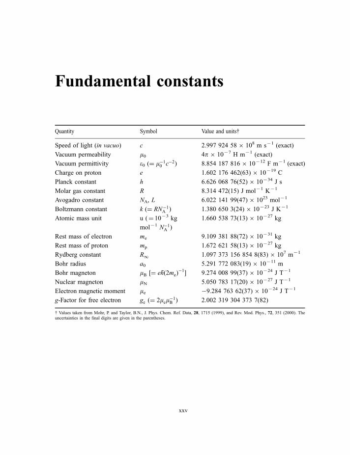
Fundamental constants
Quantity Symbol Value and unitsy
Speed of light (in vacuo) c 2.997 924 586 108 m s71 (exact)
Vacuum permeability m0 4p6 1077 H m71 (exact)
Vacuum permittivity e0 (¼ m�10 c�2Þ 8.854 187 8166 10712 F m71 (exact)
Charge on proton e 1.602 176 462(63)6 10719 C
Planck constant h 6.626 068 76(52)6 10734 J s
Molar gas constant R 8.314 472(15) J mol71 K71
Avogadro constant NA, L 6.022 141 99(47)6 1023 mol71
Boltzmann constant k (¼ RN�1A Þ 1.380 650 3(24)6 10723 J K71
Atomic mass unit u (¼ 1073 kg
mol71 N�1A )
1.660 538 73(13)6 10727 kg
Rest mass of electron me 9.109 381 88(72)6 10731 kg
Rest mass of proton mp 1.672 621 58(13)6 10727 kg
Rydberg constant R1 1.097 373 156 854 8(83)6 107 m71
Bohr radius a0 5.291 772 083(19)6 10711 m
Bohr magneton mB ½¼ e �hð2meÞ�1� 9.274 008 99(37)6 10724 J T71
Nuclear magneton mN 5.050 783 17(20)6 10727 J T71
Electron magnetic moment me �9.284 763 62(37)6 10724 J T71
g-Factor for free electron ge ð¼ 2mem�1B Þ 2.002 319 304 373 7(82)
y Values taken from Mohr, P. and Taylor, B.N., J. Phys. Chem. Ref. Data, 28, 1715 (1999), and Rev. Mod. Phys., 72, 351 (2000). Theuncertainties in the final digits are given in the parentheses.
xxv

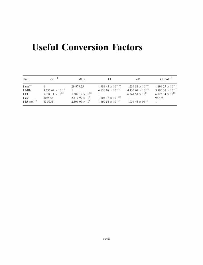
Useful Conversion Factors
Unit cm71 MHz kJ eV kJ mol71
1 cm71 1 29 979.25 1.986 456 10726 1.239 846 1074 1.196 276 1072
1 MHz 3.335 646 1075 1 6.626 086 10731 4.135 676 1079 3.990 316 1077
1 kJ 5.034 116 1025 1.509 196 1030 1 6.241 516 1021 6.022 146 1023
1 eV 8065.54 2.417 996 108 1.602 186 10722 1 96.485
1 kJ mol71 83.5935 2.506 076 106 1.660 546 10724 1:036 43� 10�2 1
xxvii

MODERNSPECTROSCOPY
Fourth Edition
J. Michael HollasUniversity of Reading

1Some Important Results inQuantum Mechanics
1.1 Spectroscopy and quantum mechanics
Spectroscopy is basically an experimental subject and is concerned with the absorption,
emission or scattering of electromagnetic radiation by atoms or molecules. As we shall see
in Chapter 3, electromagnetic radiation covers a wide wavelength range, from radio waves to
g-rays, and the atoms or molecules may be in the gas, liquid or solid phase or, of great
importance in surface chemistry, adsorbed on a solid surface.
Quantum mechanics, in contrast, is a theoretical subject relating to many aspects of
chemistry and physics, but particularly to spectroscopy.
Experimental methods of spectroscopy began in the more accessible visible region of the
electromagnetic spectrum where the eye could be used as the detector. In 1665 Newton had
started his famous experiments on the dispersion of white light into a range of colours using
a triangular glass prism. However, it was not until about 1860 that Bunsen and Kirchhoff
began to develop the prism spectroscope as an integrated unit for use as an analytical
instrument. Early applications were the observation of the emission spectra of various
samples in a flame, the origin of flame tests for various elements, and of the sun.
The visible spectrum of atomic hydrogen had been observed both in the solar spectrum
and in an electrical discharge in molecular hydrogen many years earlier, but it was not until
1885 that Balmer fitted the resulting series of lines to a mathematical formula. In this way
began the close relationship between experiment and theory in spectroscopy, the
experiments providing the results and the relevant theory attempting to explain them and
to predict results in related experiments. However, theory ran increasingly into trouble as it
was based on classical newtonian mechanics until, from 1926 onwards, Schrodinger
developed quantum mechanics. Even after this breakthrough, the importance of which
cannot be overstressed, it is not, I think, unfair to say that theory tended to limp along behind
experiment. Data from spectroscopic experiments, except for those on the simplest atoms
and molecules, were easily able to outstrip the predictions of theory, which was almost
always limited by the approximations that had to be made in order that the calculations be
manageable. It was only from about 1960 onwards that the situation changed as a result of
the availability of large, fast computers requiring many fewer approximations to be made.
Nowadays it is not uncommon for predictions to be made of spectroscopic and structural
1
properties of fairly small molecules that are comparable in accuracy to those obtainable from
experiment.
Although spectroscopy and quantum mechanics are closely interrelated it is nevertheless
the case that there is still a tendency to teach the subjects separately while drawing attention
to the obvious overlap areas. This is the attitude I shall adopt in this book, which is
concerned primarily with the techniques of spectroscopy and the interpretation of the data
that accrue. References to texts on quantum mechanics are given in the bibliography at the
end of this chapter.
1.2 The evolution of quantum theory
During the late nineteenth century evidence began to accumulate that classical newtonian
mechanics, which was completely successful on a macroscopic scale, was unsuccessful
when applied to problems on an atomic scale.
In 1885 Balmer was able to fit the discrete wavelengths l of part of the emission spectrum
of the hydrogen atom, now called the Balmer series and illustrated in Figure 1.1, to the
empirical formula
l ¼ n02Gn02 � 4
ð1:1Þ
where G is a constant and n0 ¼ 3; 4; 5; . . . : In this figure the wavenumber1 ~nn and the
wavelength l are used: the two are related by
~nn ¼ 1
lð1:2Þ
Using the relationship
n ¼ c
lð1:3Þ
where n is the frequency and c the speed of light in a vacuum, Equation (1.1) becomes
n ¼ RH
1
22� 1
n02
� �ð1:4Þ
in which RH is the Rydberg constant for hydrogen. This equation, and even the fact that
the spectrum is discrete rather than continuous, is completely at variance with classical
mechanics.
Another phenomenon that was inexplicable in classical terms was the photoelectric effect
discovered by Hertz in 1887. When ultraviolet light falls on an alkali metal surface, electrons
are ejected from the surface only when the frequency of the radiation reaches the threshold
1 See Units, dimensions and conventions on p. xxii.
2 1 SOME IMPORTANT RESULTS IN QUANTUM MECHANICS
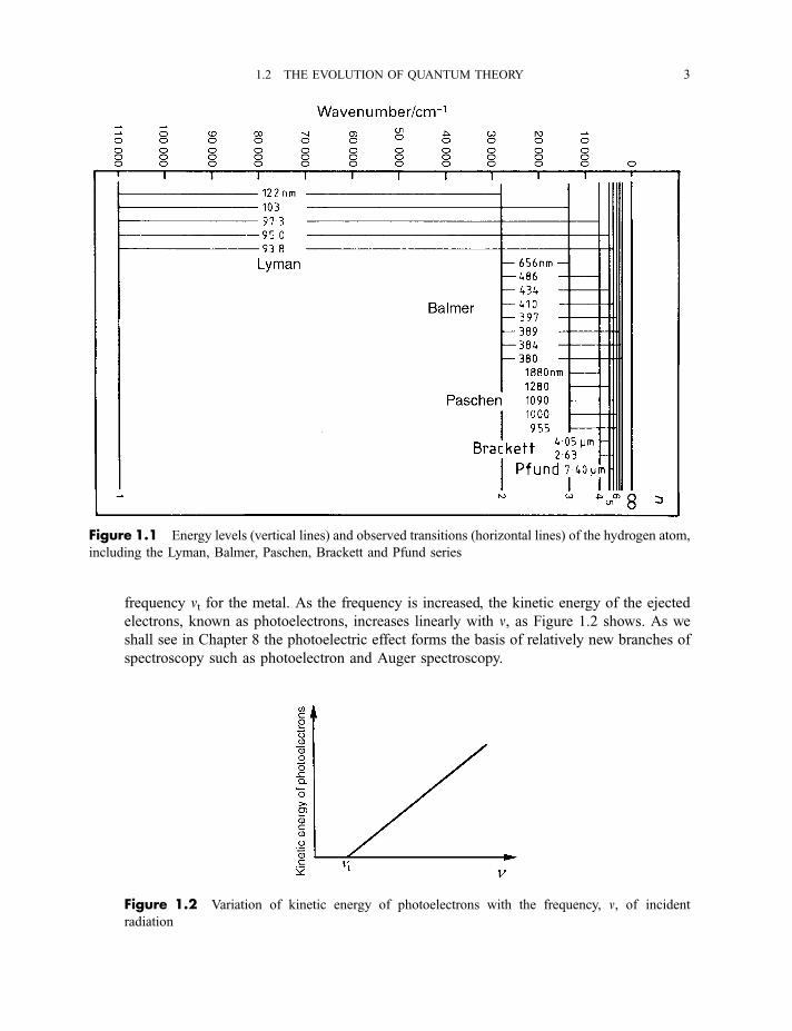
frequency nt for the metal. As the frequency is increased, the kinetic energy of the ejected
electrons, known as photoelectrons, increases linearly with n, as Figure 1.2 shows. As we
shall see in Chapter 8 the photoelectric effect forms the basis of relatively new branches of
spectroscopy such as photoelectron and Auger spectroscopy.
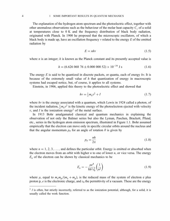
Figure 1.1 Energy levels (vertical lines) and observed transitions (horizontal lines) of the hydrogen atom,
including the Lyman, Balmer, Paschen, Brackett and Pfund series
Figure 1.2 Variation of kinetic energy of photoelectrons with the frequency, n, of incident
radiation
1.2 THE EVOLUTION OF QUANTUM THEORY 3
The explanation of the hydrogen atom spectrum and the photoelectric effect, together with
other anomalous observations such as the behaviour of the molar heat capacity Cv of a solid
at temperatures close to 0 K and the frequency distribution of black body radiation,
originated with Planck. In 1900 he proposed that the microscopic oscillators, of which a
black body is made up, have an oscillation frequency n related to the energy E of the emitted
radiation by
E ¼ nhn ð1:5Þ
where n is an integer; h is known as the Planck constant and its presently accepted value is
h ¼ ð6:626 068 76� 0:000 000 52Þ � 10�34 J s ð1:6Þ
The energy E is said to be quantized in discrete packets, or quanta, each of energy hn. It isbecause of the extremely small value of h that quantization of energy in macroscopic
systems had escaped notice, but, of course, it applies to all systems.
Einstein, in 1906, applied this theory to the photoelectric effect and showed that
hn ¼ 12mev2 þ I ð1:7Þ
where hn is the energy associated with a quantum, which Lewis in 1924 called a photon, of
the incident radiation, 12mev2 is the kinetic energy of the photoelectron ejected with velocity
v, and I is the ionization energy2 of the metal surface.
In 1913 Bohr amalgamated classical and quantum mechanics in explaining the
observation of not only the Balmer series but also the Lyman, Paschen, Brackett, Pfund,
etc., series in the hydrogen atom emission spectrum, illustrated in Figure 1.1. Bohr assumed
empirically that the electron can move only in specific circular orbits around the nucleus and
that the angular momentum py for an angle of rotation y is given by
py ¼nh
2pð1:8Þ
where n ¼ 1; 2; 3; . . . ; and defines the particular orbit. Energy is emitted or absorbed when
the electron moves from an orbit with higher n to one of lower n, or vice versa. The energy
En of the electron can be shown by classical mechanics to be
En ¼ �me4
8h2e20
1
n2
� �ð1:9Þ
where m, equal to memp=ðme þ mpÞ, is the reduced mass of the system of electron e plus
proton p, e is the electronic charge, and e0 the permittivity of a vacuum. These are the energy
2 I is often, but strictly incorrectly, referred to as the ionization potential, although, for a solid, it is
usually called the work function.
4 1 SOME IMPORTANT RESULTS IN QUANTUM MECHANICS
levels in Figure 1.1 except that ~nn, equal to En=hc, rather than En, is plotted. The zero of
energy is taken to correspond to n¼?, at which level the atom is ionized.3 The energy
levels are discrete below n¼? but continuous above it since the electron can be ejected
with any amount of kinetic energy.
When the electron transfers from, say, a lower n00 to an upper n0 orbit4 the energy DErequired is, from equation (1.9),
DE ¼ me4
8h2e20
1
n002� 1
n02
� �ð1:10Þ
or, since DE ¼ hn, we have, in terms of frequency,
n ¼ me4
8h3e20
1
n002� 1
n02
� �ð1:11Þ
Comparison with the empirical Equation (1.4) shows that RH ¼ me4=8h3e20 and that n00 ¼ 2
for the Balmer series. Similarly n00 ¼ 1; 3, 4, and 5 for the Lyman, Paschen, Brackett and
Pfund series, although it is important to realize that there is an infinite number of series.
Many series with high n00 have been observed, by techniques of radioastronomy, in the
interstellar medium, where there is a large amount of atomic hydrogen. For example, the
ðn0 ¼ 167Þ � ðn00 ¼ 166Þ transition5 has been observed with n¼ 1.425 GHz (l¼ 21.04 cm).
The Rydberg constant from Equation (1.11) has dimensions of frequency but is more
often quoted with dimensions of wavenumber when
~RRH ¼me4
8h3e20c¼ 1:096 776� 107 m�1 ð1:12Þ
Worked example1.1
Question. Using Equations (1.11) and (1.12) calculate, to six significant figures, the
wavenumbers, in cm71, of the first two (lowest n00) members of the Balmer series of the
hydrogen atom. Then convert these to wavelengths, in nm.
Answer. With dimensions of wavenumber, rather than frequency, Equation (1.11) becomes
~nn ¼ ~RRH
1
n002� 1
n02
� �
3 Note that, when A!Aþþ e, it is the atom A, not the electron, that is ionized.4 The use of single (0) and double (00) primes to indicate the upper and lower states, respectively, of a
transition is general in spectroscopy and will apply throughout the book.5 The use of U7L to indicate a transition between an upper state U and a lower state L is general in
spectroscopy and will apply throughout the book.
1.2 THE EVOLUTION OF QUANTUM THEORY 5
For the Balmer series, n00 ¼ 2 and, for the first two members, n0 ¼ 3 and 4. Their wavenumbers
are given as follows. For n0 ¼ 3:
~nn ¼ 1:096 776� 105ð14� 1
9Þ cm�1
¼ 1:096 776� 105 � 0:138 888 9 cm�1
¼ 15 233:00 cm�1
l ¼ 1
~nn¼ 6:564 695� 10�5 cm
¼ 656:470 nm
For n0 ¼ 4:
~nn ¼ 1:096 776� 105ð14� 1
16Þ cm�1
¼ 1:096 776� 105 � 0:187 500 0 cm�1
¼ 20 564:55 cm�1
l ¼ 1
~nn¼ 4:862 737� 10�5 cm
¼ 486:274 nm
Note that seven figures are retained in the calculation until the final stage, when the numbers are
rounded to six significant figures.
Planck’s quantum theory was very successful in explaining the hydrogen atom spectrum,
the wavelength distribution of black body radiation, the photoelectric effect and the low-
temperature heat capacities of solids, but it also gave rise to apparent anomalies. One of
these concerned the photoelectric effect in which the ultraviolet light falling on an alkali
metal surface behaves as if it consists of particles, whereas the phenomena of interference
and diffraction of light are explained by its wave nature. This dual wave-particle nature,
which applies not only to light but also to any particle or radiation, was resolved by de
Broglie in 1924. He proposed that
p ¼ h
lð1:13Þ
relating the momentum p in the particle picture to the wavelength l in the wave picture. Thisequation led, for example, to the important prediction that a beam of electrons, travelling
with uniform velocity, and therefore momentum, should show wave-like properties. In 1925
Davisson and Germer confirmed this by showing that the surface of crystalline nickel
reflected and diffracted a monochromatic electron beam. Their experiment formed the basis
of the LEED (low-energy electron diffraction) technique for investigating structure near the
surface of crystalline materials. Further experiments showed that transmission of an electron
beam through a thin metal foil also resulted in diffraction. Using a gaseous, rather than a
6 1 SOME IMPORTANT RESULTS IN QUANTUM MECHANICS
solid, sample the technique of electron diffraction is an important method of determining
molecular geometry in a way that is complementary to spectroscopic methods.
Now that the wave and particle pictures were reconciled it became clear why the electron
in the hydrogen atom may be only in particular orbits with angular momentum given by
Equation (1.8). In the wave picture the circumference 2pr of an orbit of radius r must
contain an integral number of wavelengths
nl ¼ 2pr ð1:14Þ
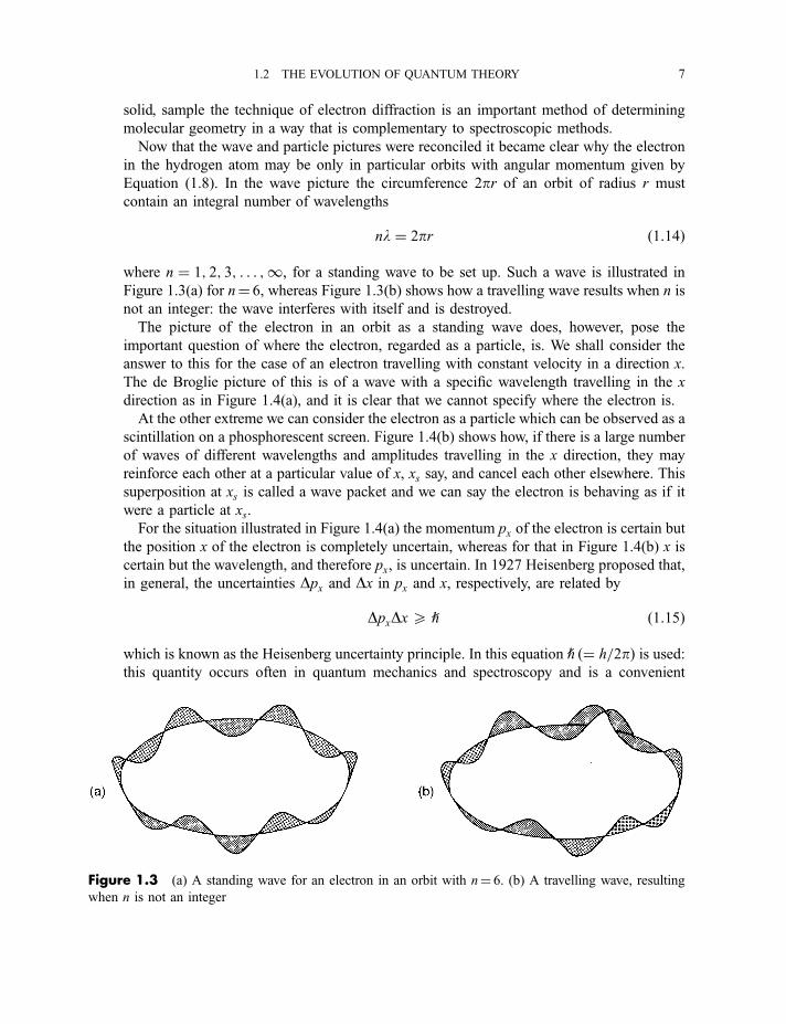
where n ¼ 1; 2; 3; . . . ;1, for a standing wave to be set up. Such a wave is illustrated in
Figure 1.3(a) for n¼ 6, whereas Figure 1.3(b) shows how a travelling wave results when n is
not an integer: the wave interferes with itself and is destroyed.
The picture of the electron in an orbit as a standing wave does, however, pose the
important question of where the electron, regarded as a particle, is. We shall consider the
answer to this for the case of an electron travelling with constant velocity in a direction x.
The de Broglie picture of this is of a wave with a specific wavelength travelling in the x
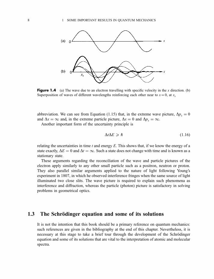
direction as in Figure 1.4(a), and it is clear that we cannot specify where the electron is.
At the other extreme we can consider the electron as a particle which can be observed as a
scintillation on a phosphorescent screen. Figure 1.4(b) shows how, if there is a large number
of waves of different wavelengths and amplitudes travelling in the x direction, they may
reinforce each other at a particular value of x, xs say, and cancel each other elsewhere. This
superposition at xs is called a wave packet and we can say the electron is behaving as if it
were a particle at xs.
For the situation illustrated in Figure 1.4(a) the momentum px of the electron is certain but
the position x of the electron is completely uncertain, whereas for that in Figure 1.4(b) x is
certain but the wavelength, and therefore px, is uncertain. In 1927 Heisenberg proposed that,
in general, the uncertainties Dpx and Dx in px and x, respectively, are related by
DpxDx 5 h ð1:15Þ
which is known as the Heisenberg uncertainty principle. In this equation h ð¼ h=2pÞ is used:this quantity occurs often in quantum mechanics and spectroscopy and is a convenient
Figure 1.3 (a) A standing wave for an electron in an orbit with n¼ 6. (b) A travelling wave, resulting
when n is not an integer
1.2 THE EVOLUTION OF QUANTUM THEORY 7
abbreviation. We can see from Equation (1.15) that, in the extreme wave picture, Dpx ¼ 0
and Dx ¼ 1 and, in the extreme particle picture, Dx ¼ 0 and Dpx ¼ 1.
Another important form of the uncertainty principle is
DtDE 5 h ð1:16Þ
relating the uncertainties in time t and energy E. This shows that, if we know the energy of a
state exactly, DE ¼ 0 and Dt ¼ 1. Such a state does not change with time and is known as a
stationary state.
These arguments regarding the reconciliation of the wave and particle pictures of the
electron apply similarly to any other small particle such as a positron, neutron or proton.
They also parallel similar arguments applied to the nature of light following Young’s
experiment in 1807, in which he observed interference fringes when the same source of light
illuminated two close slits. The wave picture is required to explain such phenomena as
interference and diffraction, whereas the particle (photon) picture is satisfactory in solving
problems in geometrical optics.
1.3 The Schrodinger equation and some of its solutions
It is not the intention that this book should be a primary reference on quantum mechanics:
such references are given in the bibliography at the end of this chapter. Nevertheless, it is
necessary at this stage to take a brief tour through the development of the Schrodinger
equation and some of its solutions that are vital to the interpretation of atomic and molecular
spectra.
Figure 1.4 (a) The wave due to an electron travelling with specific velocity in the x direction. (b)
Superposition of waves of different wavelengths reinforcing each other near to x¼ 0, at xs
8 1 SOME IMPORTANT RESULTS IN QUANTUM MECHANICS
1.3.1 The Schrodinger Equation
The Schrodinger equation cannot be subjected to firm proof but was put forward as a
postulate, based on the analogy between the wave nature of light and of the electron. The
equation was justified by the remarkable successes of its applications.
Just as a travelling light wave can be represented by a function of its amplitude at a
particular position and time, so it was proposed that a wave function Cðx; y; z; tÞ, a functionof position and time, describes the amplitude of an electron wave. In 1926 Born related the
wave and particle views by saying that we should speak not of a particle being at a particular
point at a particular time but of the probability of finding the particle there. This probability
is given byC*C, where C* is the complex conjugate of C obtained by replacing all i (equal
to the square root of �1) in C by �i. It follows thatðC*C dt ¼ 1 ð1:17Þ
where dt is the volume element dxdydz, because the probability of finding the electron
anywhere in space is unity. It seemed reasonable also that this probability is independent of
time:
@
ðC*C dt
� �@t
¼ 0 ð1:18Þ
which was assumed in the non-relativistic quantum mechanics of Schrodinger developed in
1926. Dirac, in 1928, showed that, when relativity is taken into account, this is not quite
true, but we shall not be concerned with the effects of relativity.
The form postulated for the wave function is
C ¼ b expiA
h
� �ð1:19Þ
where b is a constant and A is the action, which is related to the kinetic energy T and the
potential energy V by
� @A
@t¼ T þ V ¼ H ð1:20Þ
where H, the sum of the kinetic and potential energies, is known as the hamiltonian in
classical mechanics. From Equations (1.19) and (1.20) it follows that
HC ¼ i h@C@t
ð1:21Þ
1.3 THE SCHRODINGER EQUATION AND SOME OF ITS SOLUTIONS 9
Schrodinger postulated that the form of the hamiltonian in quantum mechanics is
obtained by replacing the kinetic energy in Equation (1.20), giving
H ¼ � h2
2mH2 þ V ð1:22Þ
The symbol H is called ‘del’ and in cartesian coordinates H2, known as the laplacian, is
given by
H2 ¼ @2
@x2þ @2
@y2þ @2
@z2ð1:23Þ
From Equations (1.21) and (1.22) we obtain the time-dependent Schrodinger equation
� h2
2mH2Cþ VC ¼ i h
@C@t
ð1:24Þ
but, since we shall be dealing mostly with standing waves, it is the time-independent part
which will concern us most.
We consider, for ease of manipulation, the wave travelling in the x direction and assume
that Cðx; tÞ can be factorized into a time-dependent part yðtÞ and a time-independent part
cðxÞ, giving
Cðx; tÞ ¼ cðxÞyðtÞ ð1:25Þ
Combination of Equation (1.24), for a one-dimensional system, and Equation (1.25) gives
� h2
2mcðxÞ@2cðxÞ@x2þ V ðxÞ ¼ ih
yðtÞ@yðtÞ@t
ð1:26Þ
Since the left-hand side is a function of x only and the right-hand side a function of t only,
they must both be constant. Since they have the same dimensions as V(x) (i.e. energy) we put
them equal to E. For the left-hand side this gives
� h2
2m
@2cðxÞ@x2þ V ðxÞcðxÞ ¼ EcðxÞ ð1:27Þ
which is the one-dimensional, time-independent Schrodinger equation, often simply called
the wave equation. It can be rewritten in the general form
Hc ¼ Ec ð1:28Þ
where H is the hamiltonian of Equation (1.22), but for one dimension only. Since H contains
@=@x it is, in mathematical terms, an operator as, for example, d=dx is an operator which
operates on x2 to give 2x. As a result, Equation (1.28) appears deceptively simple. It means
10 1 SOME IMPORTANT RESULTS IN QUANTUM MECHANICS
that operating on c by H gives the result of c multiplied by an energy E. A simple example
is provided by
d
dxexpð2xÞ ¼ 2 expð2xÞ ð1:29Þ
an equation of the same form as Equation (1.28).
For the quantum mechanical results that we require we shall be concerned only with
stationary states, known sometimes as eigenstates. The wave functions for these states may
be referred to as eigenfunctions and the associated energies E as the eigenvalues.
The details of the methods of solving the Schrodinger equation for c and E for various
systems do not concern us here but may be found in books listed in the bibliography. We
require only the results, some of which will now be discussed.
1.3.2 The hydrogen atom
The hydrogen atom, consisting of a proton and only one electron, occupies a very important
position in the development of quantum mechanics because the Schrodinger equation may
be solved exactly for this system. This is true also for the hydrogen-like atomic ions Heþ,Li2þ, Be3þ, etc., and simple one-electron molecular ions such as Hþ2 .In the quantum mechanical picture of the hydrogen atom the total energy En is quantized
and has exactly the same values as in Equation (1.9), derived from classical mechanics. The
angular momentum of the electron in a particular orbit, or orbital as it is called in quantum
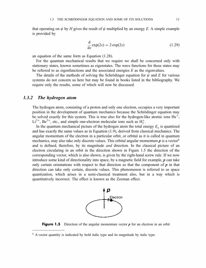
mechanics, may also take only discrete values. This orbital angular momentum p is a vector6
and is defined, therefore, by its magnitude and direction. In the classical picture of an
electron circulating in an orbit in the direction shown in Figure 1.5 the direction of the
corresponding vector, which is also shown, is given by the right-hand screw rule. If we now
introduce some kind of directionality into space, by a magnetic field for example, p can take
only certain orientations with respect to that direction so that the component of p in that
direction can take only certain, discrete values. This phenomenon is referred to as space
quantization, which arises in a semi-classical treatment also, but in a way which is
quantitatively incorrect. The effect is known as the Zeeman effect.
6 A vector quantity is indicated by bold italic type and its magnitude by italic type.
Figure 1.5 Direction of the angular momentum vector p for an electron in an orbit
1.3 THE SCHRODINGER EQUATION AND SOME OF ITS SOLUTIONS 11
For the hydrogen atom, the hamiltonian of Equation (1.22) becomes
H ¼ � h2
2mH2 � e2
4pe0rð1:30Þ
The second term on the right-hand side is the coulombic potential energy for the attraction
between charges �e and þe a distance r apart. The first term contains the reduced mass m,equal to memp=ðme þ mpÞ, for the system of an electron of mass me and a proton of mass mp.
It also contains the laplacian H2 which is here defined as
H2 ¼ 1
r2 sin ysin y
@
@rr2
@
@r
� �þ @
@ysin y
@
@y
� �þ 1
sinf@2
@f2
� �ð1:31Þ
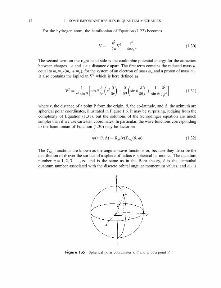
where r, the distance of a point P from the origin, y, the co-latitude, and f, the azimuth are
spherical polar coordinates, illustrated in Figure 1.6. It may be surprising, judging from the
complexity of Equation (1.31), but the solutions of the Schrodinger equation are much
simpler than if we use cartesian coordinates. In particular, the wave functions corresponding
to the hamiltonian of Equation (1.30) may be factorized:
cðr; y;fÞ ¼ Rn‘ðrÞY‘m‘ðy;fÞ ð1:32Þ
The Y‘m‘functions are known as the angular wave functions or, because they describe the
distribution of c over the surface of a sphere of radius r, spherical harmonics. The quantum
number n ¼ 1; 2; 3; . . . ;1 and is the same as in the Bohr theory, ‘ is the azimuthal
quantum number associated with the discrete orbital angular momentum values, and m‘ is
Figure 1.6 Spherical polar coordinates r, y and f of a point P
12 1 SOME IMPORTANT RESULTS IN QUANTUM MECHANICS
known as the magnetic quantum number which results from the space quantization of the
orbital angular momentum. These quantum numbers can take the values
‘ ¼ 0; 1; 2; . . . ; ðn� 1Þ ð1:33Þm‘ ¼ 0;�1;�2; . . . ;�‘ ð1:34Þ
The function Y‘m‘ðy;fÞ in Equation (1.32) can be factorized further to give
Y‘m‘ðy;fÞ ¼ ð2pÞ�1=2Y‘m‘
ðyÞ expðim‘fÞ ð1:35Þ
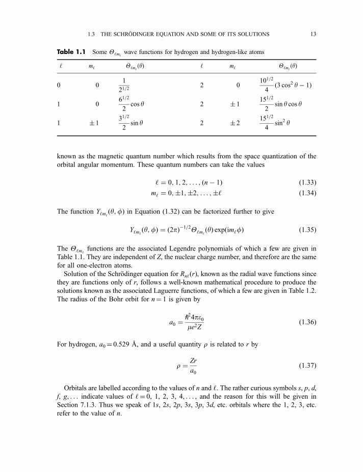
The Y‘m‘functions are the associated Legendre polynomials of which a few are given in
Table 1.1. They are independent of Z, the nuclear charge number, and therefore are the same
for all one-electron atoms.
Solution of the Schrodinger equation for Rn‘ðrÞ, known as the radial wave functions since
they are functions only of r, follows a well-known mathematical procedure to produce the
solutions known as the associated Laguerre functions, of which a few are given in Table 1.2.
The radius of the Bohr orbit for n¼ 1 is given by
a0 ¼h24pe0me2Z
ð1:36Þ
For hydrogen, a0¼ 0.529 A, and a useful quantity r is related to r by
r ¼ Zr
a0ð1:37Þ
Orbitals are labelled according to the values of n and ‘. The rather curious symbols s, p, d,
f, g, . . . indicate values of ‘¼ 0, 1, 2, 3, 4, . . . , and the reason for this will be given in
Section 7.1.3. Thus we speak of 1s, 2s, 2p, 3s, 3p, 3d, etc. orbitals where the 1, 2, 3, etc.
refer to the value of n.
Table 1.1 Some Y‘m‘wave functions for hydrogen and hydrogen-like atoms
‘ m‘ Y‘m‘ðyÞ ‘ m‘ Y‘m‘
ðyÞ
0 01
21=22 0
101=2
4ð3 cos2 y� 1Þ
1 061=2
2cos y 2 � 1
151=2
2sin y cos y
1 � 131=2
2sin y 2 � 2
151=2
4sin2 y
1.3 THE SCHRODINGER EQUATION AND SOME OF ITS SOLUTIONS 13
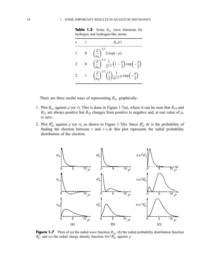
There are three useful ways of representing Rn‘ graphically:
1. Plot Rn‘ against r (or r). This is done in Figure 1.7(a), where it can be seen that R10 and
R21 are always positive but R20 changes from positive to negative and, at one value of r,is zero.
2. Plot R2n‘ against r (or r), as shown in Figure 1.7(b). Since R2
n‘ dr is the probability of
finding the electron between r and rþ dr this plot represents the radial probability
distribution of the electron.
Table 1.2 Some Rn‘ wave functions for
hydrogen and hydrogen-like atoms
n ‘ Rn‘ðrÞ
1 0Z
a0
� �3=2
2 expð�rÞ
2 0Z
a0
� �3=21
21=21� r
2
� �exp � r
2
� �
2 1Z
a0
� �3=21
2
� �1
61=2r exp � r
2
� �
Figure 1.7 Plots of (a) the radial wave function Rn‘, (b) the radial probability distribution function
R2n‘ and (c) the radial charge density function 4pr2R2
n‘ against r
14 1 SOME IMPORTANT RESULTS IN QUANTUM MECHANICS
3. Plot 4pr2R2n‘ against r (or r), as shown in Figure 1.7(c). The quantity 4pr2R2
n‘ is called
the radial charge density and is the probability of finding the electron in a volume
element consisting of a thin spherical shell of thickness dr, radius r, and volume 4pr2 dr.
Diagrammatic representations of the Y‘m‘functions in Equation (1.35) cannot be made
until we convert them from imaginary into real functions. Exceptions are the functions with
m‘ ¼ 0, which are already real.
In the absence of an electric or magnetic field all the Y‘m‘functions with ‘ 6¼ 0 are
ð2‘þ 1Þ-fold degenerate, which means that there are ð2‘þ 1Þ functions, each having one of
the ð2‘þ 1Þ possible values of m‘, with the same energy. It is a property of degenerate
functions that linear combinations of them are also solutions of the Schrodinger equation.
For example, just as c2p;1 and c2p;�1 are solutions, so are
c2px¼ 2�1=2ðc2p;1 þ c2p;�1Þ
c2py¼ �2�1=2iðc2p;1 � c2p;�1Þ
9=; ð1:38Þ
From Equations (1.32), (1.35) and (1.38), together with the Y‘m‘functions in Table 1.1, it
follows that
c2px¼ 1
2ð4pÞ1=2 R21ðrÞ31=2 sin y½expðifÞ þ expð�ifÞ�
c2py¼ 1
2ð4pÞ1=2 iR21ðrÞ31=2 sin y½expðifÞ � expð�ifÞ�
9>>>=>>>; ð1:39Þ
However, since
expðifÞ þ expð�ifÞ ¼ 2 cosf
expðifÞ � expð�ifÞ ¼ 2i sinf
�ð1:40Þ
Equations (1.39) become
c2px¼ 1
ð4pÞ1=2 R21ðrÞ31=2 sin y cosf ð1:41Þ
c2py¼ 1
ð4pÞ1=2 R21ðrÞ31=2 sin y sinf ð1:42Þ
In addition, the third degenerate c2p;0 wave function is always real, and we label it c2pz,
where
c2pz¼ 1
ð4pÞ1=2 R21ðrÞ31=2 cos y ð1:43Þ
1.3 THE SCHRODINGER EQUATION AND SOME OF ITS SOLUTIONS 15
All the cns wave functions are always real and so are the cnd , cnf , etc. wave functions for
m‘ ¼ 0. However, for cnd with m‘ ¼ �1 or �2, it is necessary to form linear combinations
of the imaginary wave functions cnd;1 and cnd;�1, or cnd;2 and cnd;�2, to obtain real
functions. The cnd orbital wave functions for any n> 2 are distinguished by subscripts
ndz2 ðm‘ ¼ 0Þ, ndxz and ndyz ðm‘ ¼ �1Þ, and ndxy and ndx2�y2 ðm‘ ¼ �2Þ. There are seven
nf orbitals for any n> 3 but we shall not consider them here.
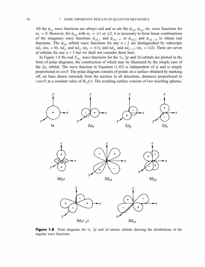
In Figure 1.8 the real Y‘m‘wave functions for the 1s, 2p and 3d orbitals are plotted in the
form of polar diagrams, the construction of which may be illustrated by the simple case of
the 2pz orbital. The wave function in Equation (1.43) is independent of f and is simply
proportional to cos y. The polar diagram consists of points on a surface obtained by marking
off, on lines drawn outwards from the nucleus in all directions, distances proportional to
j cos yj at a constant value of R21ðrÞ. The resulting surface consists of two touching spheres,
Figure 1.8 Polar diagrams for 1s, 2p and 3d atomic orbitals showing the distributions of the
angular wave functions
16 1 SOME IMPORTANT RESULTS IN QUANTUM MECHANICS
as shown in Figure 1.8, which shows polar diagrams for all 1s, 2p and 3d orbitals. Figure 1.7
shows that all Rn‘! 0 as r!1. Polar diagrams are drawn as surface boundaries within
which ca 90% of the Rn‘ wave function resides.
For all orbitals except 1s there are regions in space where cðr; y;fÞ ¼ 0 because either
Y‘m‘¼ 0 or Rn‘ ¼ 0. In these regions the electron density is zero and we call them nodal
surfaces or, simply, nodes. For example, the 2pz orbital has a nodal plane, while each of the
3d orbitals has two nodal planes. In general, there are ‘ such angular nodes where Y‘m‘¼ 0.
The 2s orbital has one spherical nodal plane, or radial node, as Figure 1.7 shows. In general,
there are (n7 1) radial nodes for an ns orbital (or n if we count the one at infinity).
Quantum mechanical solution results in the same expression for the energy levels, given
in Equation (1.9), as in the Bohr theory – indeed, it must do since the Bohr theory agrees
exactly with experiment, except for the fine structure of the spectrum, which our present
quantum mechanical treatment has not explained either. But there are far-reaching
differences in the quantum mechanical treatment. Some of these are embodied in Figures 1.7
and 1.8, which portray the electron as smeared out in various patterns of probability which
always approach zero as r tends to infinity. The probability distribution also contains nodal
surfaces where there is zero probability of finding the electron. All of this is a far cry from
the classical picture of the electron orbiting round the nucleus like the moon orbiting round
the earth.
Unlike the total energy, the quantum mechanical value P‘ of the orbital angular
momentum is significantly different from that in the Bohr theory given in Equation (1.8). It
is now given by
P‘ ¼ ½‘ð‘þ 1Þ�1=2h ð1:44Þ
where ‘ ¼ 0; 1; 2; . . . ; ðn� 1Þ, as in Equation (1.33).
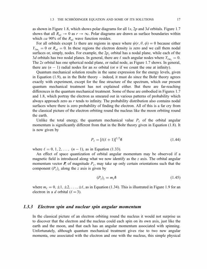
An effect of space quantization of orbital angular momentum may be observed if a
magnetic field is introduced along what we now identify as the z axis. The orbital angular
momentum vector P, of magnitude P‘, may take up only certain orientations such that the
component ðP‘Þz along the z axis is given by
ðP‘Þz ¼ m‘h ð1:45Þ
where m‘ ¼ 0;�1;�2; . . . ;�‘, as in Equation (1.34). This is illustrated in Figure 1.9 for anelectron in a d orbital (‘¼ 3).
1.3.3 Electron spin and nuclear spin angular momentum
In the classical picture of an electron orbiting round the nucleus it would not surprise us
to discover that the electron and the nucleus could each spin on its own axis, just like the
earth and the moon, and that each has an angular momentum associated with spinning.
Unfortunately, although quantum mechanical treatment gives rise to two new angular
momenta, one associated with the electron and one with the nucleus, this simple physical
1.3 THE SCHRODINGER EQUATION AND SOME OF ITS SOLUTIONS 17
picture breaks down. When we think, for example, of the wave rather than the particle
picture of the electron this breakdown is not surprising. However, in spite of this it is still
usual to speak of electron spin and nuclear spin.
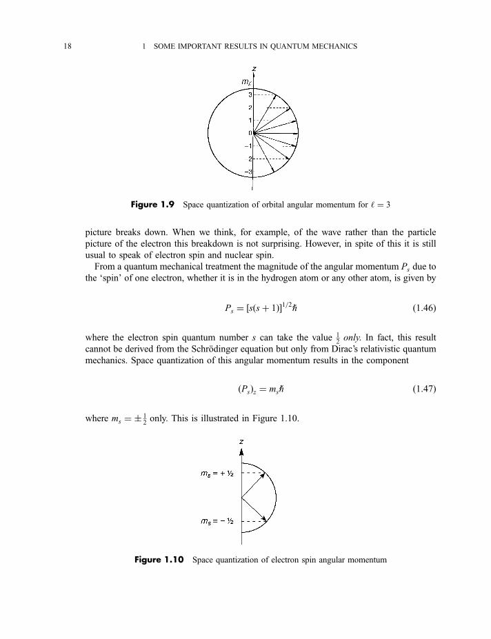
From a quantum mechanical treatment the magnitude of the angular momentum Ps due to
the ‘spin’ of one electron, whether it is in the hydrogen atom or any other atom, is given by
Ps ¼ ½sðsþ 1Þ�1=2h ð1:46Þ
where the electron spin quantum number s can take the value 12only. In fact, this result
cannot be derived from the Schrodinger equation but only from Dirac’s relativistic quantum
mechanics. Space quantization of this angular momentum results in the component
ðPsÞz ¼ msh ð1:47Þ
where ms ¼ � 12only. This is illustrated in Figure 1.10.
Figure 1.9 Space quantization of orbital angular momentum for ‘ ¼ 3
Figure 1.10 Space quantization of electron spin angular momentum
18 1 SOME IMPORTANT RESULTS IN QUANTUM MECHANICS
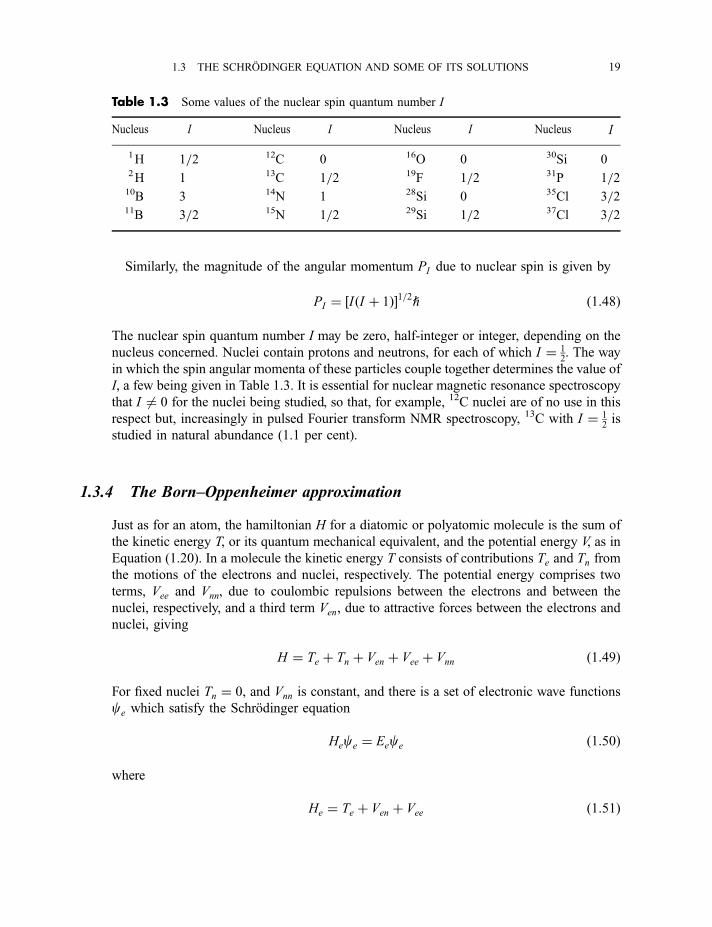
Similarly, the magnitude of the angular momentum PI due to nuclear spin is given by
PI ¼ ½I ðI þ 1Þ�1=2h ð1:48Þ
The nuclear spin quantum number I may be zero, half-integer or integer, depending on the
nucleus concerned. Nuclei contain protons and neutrons, for each of which I ¼ 12. The way
in which the spin angular momenta of these particles couple together determines the value of
I, a few being given in Table 1.3. It is essential for nuclear magnetic resonance spectroscopy
that I 6¼ 0 for the nuclei being studied, so that, for example, 12C nuclei are of no use in this
respect but, increasingly in pulsed Fourier transform NMR spectroscopy, 13C with I ¼ 12is
studied in natural abundance (1.1 per cent).
1.3.4 The Born–Oppenheimer approximation
Just as for an atom, the hamiltonian H for a diatomic or polyatomic molecule is the sum of
the kinetic energy T, or its quantum mechanical equivalent, and the potential energy V, as in
Equation (1.20). In a molecule the kinetic energy T consists of contributions Te and Tn from
the motions of the electrons and nuclei, respectively. The potential energy comprises two
terms, Vee and Vnn, due to coulombic repulsions between the electrons and between the
nuclei, respectively, and a third term Ven, due to attractive forces between the electrons and
nuclei, giving
H ¼ Te þ Tn þ Ven þ Vee þ Vnn ð1:49Þ
For fixed nuclei Tn ¼ 0, and Vnn is constant, and there is a set of electronic wave functions
ce which satisfy the Schrodinger equation
Hece ¼ Eece ð1:50Þ
where
He ¼ Te þ Ven þ Vee ð1:51Þ
Table 1.3 Some values of the nuclear spin quantum number I
Nucleus I Nucleus I Nucleus I Nucleus I
1H 1=2 12C 0 16O 0 30Si 02H 1 13C 1=2 19F 1=2 31P 1=210B 3 14N 1 28Si 0 35Cl 3=211B 3=2 15N 1=2 29Si 1=2 37Cl 3=2
1.3 THE SCHRODINGER EQUATION AND SOME OF ITS SOLUTIONS 19
Since He depends on nuclear coordinates, because of the Ven term, so do ce and Ee but, in
the Born–Oppenheimer approximation proposed in 1927, it is assumed that vibrating nuclei
move so slowly compared with electrons that ce and Ee involve the nuclear coordinates as
parameters only. The result for a diatomic molecule is that a curve (such as that in Figure
1.13, p. 24) of potential energy against internuclear distance r (or the displacement from
equilibrium) can be drawn for a particular electronic state in which Te and Vee are constant.
The Born–Oppenheimer approximation is valid because the electrons adjust instanta-
neously to any nuclear motion: they are said to follow the nuclei. For this reason Ee can be
treated as part of the potential field in which the nuclei move, so that
Hn ¼ Tn þ Vnn þ Ee ð1:52Þ
and the Schrodinger equation for nuclear motion is
Hncn ¼ Encn ð1:53Þ
It follows from the Born–Oppenheimer approximation that the total wave function c can
be factorized:
c ¼ ceðq;QÞcnðQÞ ð1:54Þ
where the q are electron coordinates and ce is a function of nuclear coordinates Q as well as
q. It follows from Equation (1.54) that
E ¼ Ee þ En ð1:55Þ
The wave function cn can be factorized further into a vibrational part cv and a rotational
part cr:
cn ¼ cvcr ð1:56Þ
for the same reasons, perhaps unexpectedly, that the hydrogen atom wave function cðr; y;fÞcan be factorized into Rn‘ðrÞ and Y‘m‘
ðy;fÞ as in Equation (1.32). From Equation (1.56) it
follows that
En ¼ Ev þ Er ð1:57Þ
so that
c ¼ cecvcr ð1:58Þ
and
E ¼ Ee þ Ev þ Er ð1:59Þ
If any atoms have nuclear spin this part of the total wave function can be factorized and the
energy treated additively. It is for these reasons that we can treat electronic, vibrational,
rotational and NMR spectroscopy separately.
20 1 SOME IMPORTANT RESULTS IN QUANTUM MECHANICS
1.3.5 The rigid rotor
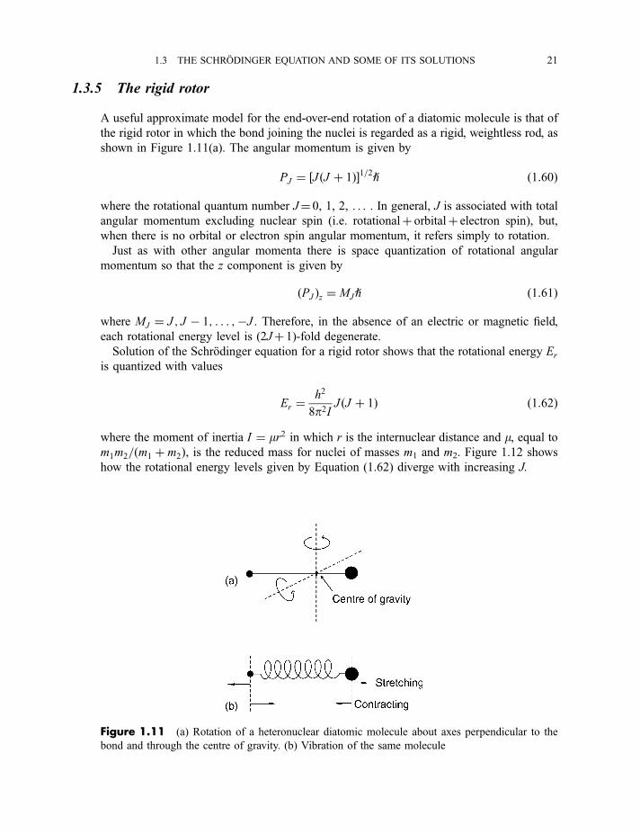
A useful approximate model for the end-over-end rotation of a diatomic molecule is that of
the rigid rotor in which the bond joining the nuclei is regarded as a rigid, weightless rod, as
shown in Figure 1.11(a). The angular momentum is given by
PJ ¼ ½J ðJ þ 1Þ�1=2h ð1:60Þ
where the rotational quantum number J¼ 0, 1, 2, . . . . In general, J is associated with total
angular momentum excluding nuclear spin (i.e. rotationalþ orbitalþ electron spin), but,
when there is no orbital or electron spin angular momentum, it refers simply to rotation.
Just as with other angular momenta there is space quantization of rotational angular
momentum so that the z component is given by
ðPJ Þz ¼ MJh ð1:61Þ
where MJ ¼ J ; J � 1; . . . ;�J . Therefore, in the absence of an electric or magnetic field,
each rotational energy level is (2Jþ 1)-fold degenerate.
Solution of the Schrodinger equation for a rigid rotor shows that the rotational energy Er
is quantized with values
Er ¼h2
8p2IJ ðJ þ 1Þ ð1:62Þ
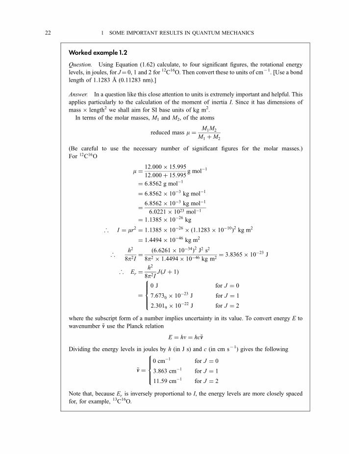
where the moment of inertia I ¼ mr2 in which r is the internuclear distance and m, equal tom1m2=ðm1 þ m2Þ, is the reduced mass for nuclei of masses m1 and m2. Figure 1.12 shows
how the rotational energy levels given by Equation (1.62) diverge with increasing J.
Figure 1.11 (a) Rotation of a heteronuclear diatomic molecule about axes perpendicular to the
bond and through the centre of gravity. (b) Vibration of the same molecule
1.3 THE SCHRODINGER EQUATION AND SOME OF ITS SOLUTIONS 21
Worked example1.2
Question. Using Equation (1.62) calculate, to four significant figures, the rotational energy
levels, in joules, for J¼ 0, 1 and 2 for 12C16O. Then convert these to units of cm71. [Use a bond
length of 1.1283 A (0.11283 nm).]
Answer. In a question like this close attention to units is extremely important and helpful. This
applies particularly to the calculation of the moment of inertia I. Since it has dimensions of
mass6 length2 we shall aim for SI base units of kg m2.
In terms of the molar masses, M1 and M2, of the atoms
reduced mass m ¼ M1M2
M1 þM2
(Be careful to use the necessary number of significant figures for the molar masses.)
For 12C16O
m ¼ 12:000� 15:995
12:000þ 15:995g mol�1
¼ 6:8562 g mol�1
¼ 6:8562� 10�3 kg mol�1
¼ 6:8562� 10�3 kg mol�1
6:0221� 1023 mol�1
¼ 1:1385� 10�26 kg
; I ¼ mr2 ¼ 1:1385� 10�26 � ð1:1283� 10�10Þ2 kg m2
¼ 1:4494� 10�46 kg m2
;h2
8p2I¼ ð6:6261� 10�34Þ2 J2 s2
8p2 � 1:4494� 10�46 kg m2¼ 3:8365� 10�23 J
; Er ¼h2
8p2IJ ðJ þ 1Þ
0 J for J ¼ 0
7:6730 � 10�23 J for J ¼ 1
2:3019 � 10�22 J for J ¼ 2
where the subscript form of a number implies uncertainty in its value. To convert energy E to
wavenumber ~nn use the Planck relation
E ¼ hn ¼ hc~nn
Dividing the energy levels in joules by h (in J s) and c (in cm s71) gives the following
0 cm�1 for J ¼ 0
3:863 cm�1 for J ¼ 1
11:59 cm�1 for J ¼ 2
Note that, because Er is inversely proportional to I, the energy levels are more closely spaced
for, for example, 13C16O.
¼
8>><>>:
~nn ¼
8>><>>:
22 1 SOME IMPORTANT RESULTS IN QUANTUM MECHANICS
1.3.6 The harmonic oscillator
Figure 1.11(b) illustrates the ball-and-spring model which is adequate for an approximate
treatment of the vibration of a diatomic molecule. For small displacements the stretching and
compression of the bond, represented by the spring, obeys Hooke’s law:
Restoring force ¼ � dV ðxÞdx¼ �kx ð1:63Þ
where V is the potential energy, k is the force constant, the magnitude of which reflects the
strength of the bond, and x, equal to r � re, is the displacement from the equilibrium bond
length re. Integration of this equation gives
V ðxÞ ¼ 12kx2 ð1:64Þ
In Figure 1.13, V ðrÞ is plotted against r and illustrates the parabolic relationship.
The quantum mechanical hamiltonian for a one-dimensional harmonic oscillator is given
by
H ¼ � h2
2md2
dx2þ 1
2kx2 ð1:65Þ
Figure 1.12 A set of rotational energy levels Er
1.3 THE SCHRODINGER EQUATION AND SOME OF ITS SOLUTIONS 23
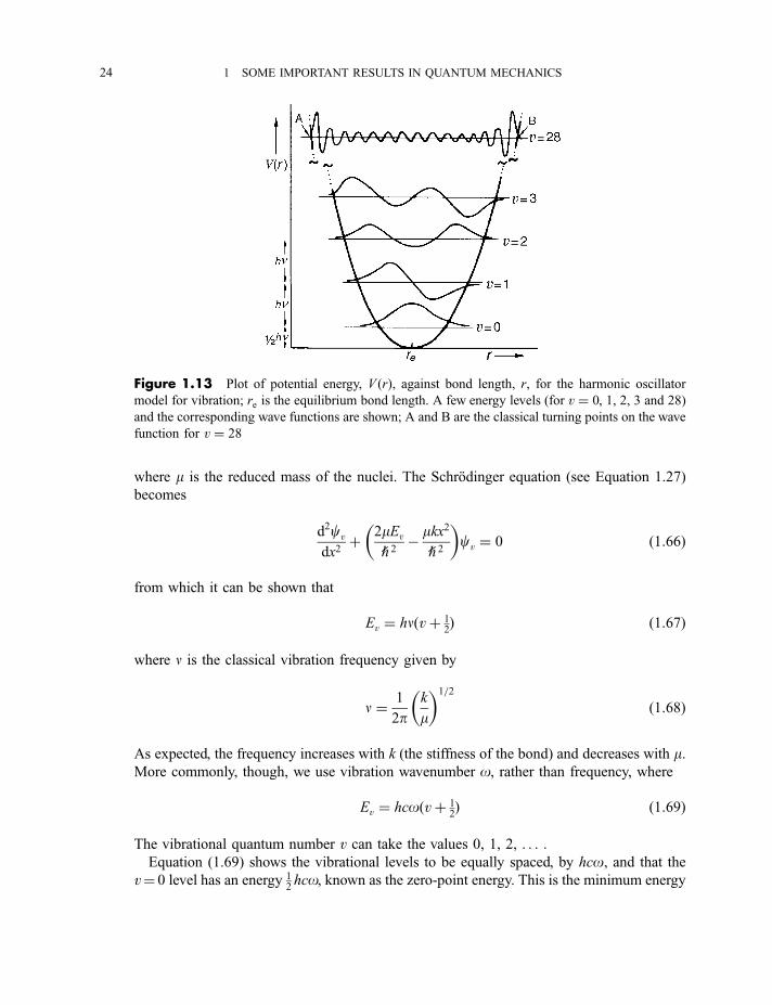
where m is the reduced mass of the nuclei. The Schrodinger equation (see Equation 1.27)
becomes
d2cv
dx2þ 2mEv
h 2� mkx2
h 2
� �cv ¼ 0 ð1:66Þ
from which it can be shown that
Ev ¼ hnðvþ 12Þ ð1:67Þ
where n is the classical vibration frequency given by
n ¼ 1
2pk
m
� �1=2
ð1:68Þ
As expected, the frequency increases with k (the stiffness of the bond) and decreases with m.More commonly, though, we use vibration wavenumber o, rather than frequency, where
Ev ¼ hcoðvþ 12Þ ð1:69Þ
The vibrational quantum number v can take the values 0, 1, 2, . . . .
Equation (1.69) shows the vibrational levels to be equally spaced, by hco, and that the
v¼ 0 level has an energy 12hco, known as the zero-point energy. This is the minimum energy
Figure 1.13 Plot of potential energy, V ðrÞ, against bond length, r, for the harmonic oscillator
model for vibration; re is the equilibrium bond length. A few energy levels (for v ¼ 0, 1, 2, 3 and 28)
and the corresponding wave functions are shown; A and B are the classical turning points on the wave
function for v ¼ 28
24 1 SOME IMPORTANT RESULTS IN QUANTUM MECHANICS
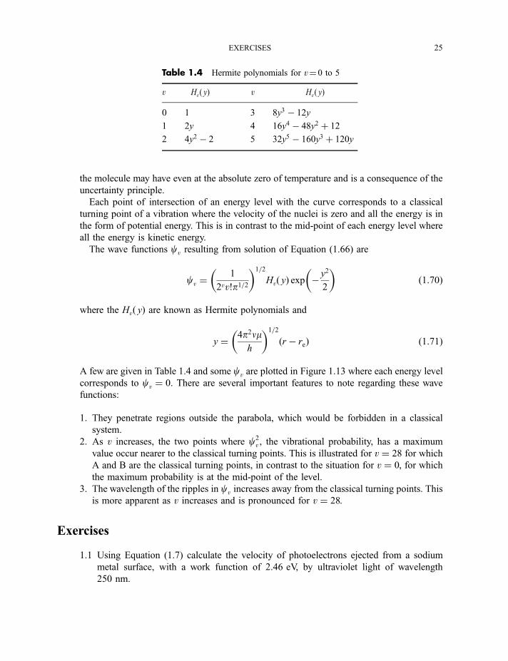
the molecule may have even at the absolute zero of temperature and is a consequence of the
uncertainty principle.
Each point of intersection of an energy level with the curve corresponds to a classical
turning point of a vibration where the velocity of the nuclei is zero and all the energy is in
the form of potential energy. This is in contrast to the mid-point of each energy level where
all the energy is kinetic energy.
The wave functions cv resulting from solution of Equation (1.66) are
cv ¼1
2vv!p1=2
� �1=2
Hvð yÞ exp �y2
2
� �ð1:70Þ
where the Hvð yÞ are known as Hermite polynomials and
y ¼ 4p2nmh
� �1=2
ðr � reÞ ð1:71Þ
A few are given in Table 1.4 and some cv are plotted in Figure 1.13 where each energy level
corresponds to cv ¼ 0. There are several important features to note regarding these wave
functions:
1. They penetrate regions outside the parabola, which would be forbidden in a classical
system.
2. As v increases, the two points where c2v , the vibrational probability, has a maximum
value occur nearer to the classical turning points. This is illustrated for v ¼ 28 for which
A and B are the classical turning points, in contrast to the situation for v ¼ 0, for which
the maximum probability is at the mid-point of the level.
3. The wavelength of the ripples in cv increases away from the classical turning points. This
is more apparent as v increases and is pronounced for v ¼ 28.
Exercises
1.1 Using Equation (1.7) calculate the velocity of photoelectrons ejected from a sodium
metal surface, with a work function of 2.46 eV, by ultraviolet light of wavelength
250 nm.
Table 1.4 Hermite polynomials for v¼ 0 to 5
v Hvð yÞ v Hvð yÞ
0 1 3 8y3 � 12y
1 2y 4 16y4 � 48y2 þ 12
2 4y2 � 2 5 32y5 � 160y3 þ 120y
EXERCISES 25

1.2 Show that the wavelength l associated with a beam of electrons accelerated by a
potential difference V is given by l ¼ hð2eVmeÞ�1=2. Calculate the wavelength of such a
beam for an accelerating potential difference of 36.20 kV.
1.3 From the Heisenberg uncertainty principle as stated in Equation (1.16) estimate, in
cm71 and Hz, the wavenumber and frequency spread of pulsed radiation with a pulse
length of 30 fs, typical of a very short pulse from a visible laser, and of 6 ms, typical ofpulsed radiofrequency radiation used in a pulsed Fourier transform NMR experiment.
1.4 Using Equation (1.36) calculate, to six significant figures, the radius of the n¼ 1 Bohr
orbit for Be3þ.
1.5 Given that the vibration wavenumbers of the molecules HCl, SO and PN are 2991, 1149
and 1337 cm71, respectively, calculate, from Equation (1.68), their force constants and
hence comment on the comparative bond strengths.
Bibliography
Atkins, P. W. (1991) Quanta: A Handbook of Concepts, Oxford University Press, Oxford.
Atkins, P. W. and Friedman, R. S. (1996) Molecular Quantum Mechanics, Oxford University Press,
Oxford.
Bockhoff, F. J. (1976) Elements of Quantum Theory, Longman Higher Education, Harlow.
Feynman, R. P., Leighton, R. B. and Sands, M. L. (1989) The Feynman Lectures on Physics:
Commemorative Issue, Addison-Wesley, Reading, MA.
Griffiths, D. J. (1995) Introduction to Quantum Mechanics, Prentice Hall, New Jersey.
Kauzmann, W. (1957) Quantum Chemistry, Academic Press, New York.
Landau, L. D. and Lifshitz, E. M. (1959) Quantum Mechanics, Pergamon Press, Oxford.
Pauling, L. (1985) Introduction to Quantum Mechanics, Dover, New York.
Schutte, C. J. H. (1968) The Wave Mechanics of Atoms, Molecules and Ions, Arnold, London.
26 1 SOME IMPORTANT RESULTS IN QUANTUM MECHANICS
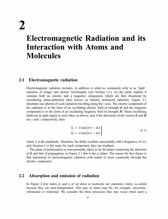
2Electromagnetic Radiation and itsInteraction with Atoms andMolecules
2.1 Electromagnetic radiation
Electromagnetic radiation includes, in addition to what we commonly refer to as ‘light’,
radiation of longer and shorter wavelengths (see Section 3.1). As the name implies it
contains both an electric and a magnetic component, which are best illustrated by
considering plane-polarized (also known as linearly polarized) radiation. Figure 2.1
illustrates one photon of such radiation travelling along the x axis. The electric component of
the radiation is in the form of an oscillating electric field of strength E and the magnetic
component is in the form of an oscillating magnetic field of strength H. These oscillating
fields are at right angles to each other, as shown, and, if the directions of the vectors E and H
are y and z respectively, then
Ey ¼ A sinð2pnt � kxÞHz ¼ A sinð2pnt � kxÞ
)ð2:1Þ
where A is the amplitude. Therefore, the fields oscillate sinusoidally with a frequency of 2pnand, because k is the same for each component, they are in-phase.
The plane of polarization is conventionally taken to be the plane containing the direction
of E and that of propagation; in Figure 2.1 this is the xy plane. The reason for this choice is
that interaction of electromagnetic radiation with matter is more commonly through the
electric component.
2.2 Absorption and emission of radiation
In Figure 2.2(a) states m and n of an atom or molecule are stationary states, so-called
because they are time-independent. This pair of states may be, for example, electronic,
vibrational or rotational. We consider the three processes that may occur when such a
27
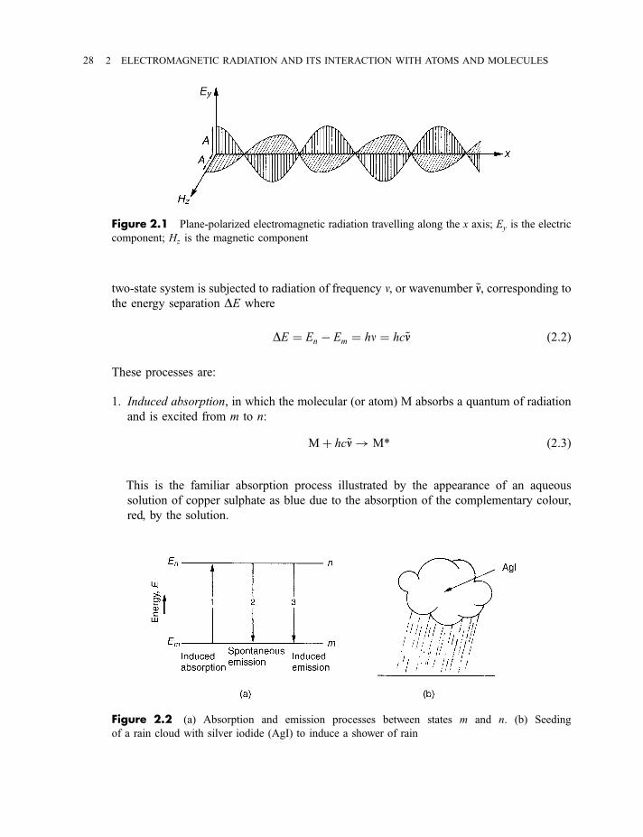
two-state system is subjected to radiation of frequency n, or wavenumber ~nn, corresponding tothe energy separation DE where
DE ¼ En � Em ¼ hn ¼ hc~nn ð2:2Þ
These processes are:
1. Induced absorption, in which the molecular (or atom) M absorbs a quantum of radiation
and is excited from m to n:
Mþ hc~nn! M* ð2:3Þ
This is the familiar absorption process illustrated by the appearance of an aqueous
solution of copper sulphate as blue due to the absorption of the complementary colour,
red, by the solution.
Figure 2.1 Plane-polarized electromagnetic radiation travelling along the x axis; Ey is the electric
component; Hz is the magnetic component
Figure 2.2 (a) Absorption and emission processes between states m and n. (b) Seeding
of a rain cloud with silver iodide (AgI) to induce a shower of rain
28 2 ELECTROMAGNETIC RADIATION AND ITS INTERACTION WITH ATOMS AND MOLECULES
2. Spontaneous emission, in which M* (in state n) spontaneously emits a quantum of
radiation:
M*! Mþ hc~nn ð2:4Þ
Almost all emission that we usually encounter, such as that from a sodium vapour or
tungsten filament lamp, is of the spontaneous type.
3. Induced, or stimulated, emission. This is a different type of emission process from that of
type 2 in that a quantum of radiation of wavenumber ~nn given by Equation (2.2) is requiredto induce, or stimulate, M* to go from n to m. The process is represented by
M*þ hc~nn! Mþ 2hc~nn ð2:5Þ
and may seem rather unusual to anyone used only to the spontaneous emission process.
There is a useful analogy between induced emission, requiring the presence of radiation
of the correct wavenumber for it to occur, and the seeding of a cloud with silver iodide
crystals in order to induce it to shed a shower of rain which it would not otherwise do, as
shown in Figure 2.2(b). The silver iodide plays the part of the quantum of radiation
necessary to induce the process. The reason why the absorption process is strictly
referred to as induced absorption may now be appreciated since, of course, it requires the
presence of radiation of wavenumber ~nn in order to occur.
The rate of change of population Nn of state n due to induced absorption is given by
dNn
dt¼ NmBmnrð~nnÞ ð2:6Þ
where Bmn is a so-called Einstein coefficient and rð~nnÞ, the spectral radiation density, is given
by
rð~nnÞ ¼ 8phc~nn3
expðhc~nn=kT Þ � 1ð2:7Þ
Similarly, induced emission changes the population Nn by
dNn
dt¼ �NnBnmrð~nnÞ ð2:8Þ
where Bnm is the Einstein coefficient for this process and is equal to Bmn. For spontaneous
emission, we have
dNn
dt¼ �NnAnm ð2:9Þ
2.2 ABSORPTION AND EMISSION OF RADIATION 29
where Anm is another Einstein coefficient and the absence of rð~nnÞ indicates a spontaneous
process. In the presence of radiation of wavenumber ~nn all three processes are going on at
once and, when the populations have reached their equilibrium values, we have
dNn
dt¼ ðNm � NnÞBnmrð~nnÞ � NnAnm ¼ 0 ð2:10Þ
At equilibrium Nn and Nm are related, through the Boltzmann distribution law, by
Nn
Nm
¼ gn
gmexp �DE
kT
� �¼ exp �DE
kT
� �ð2:11Þ
if the degrees of degeneracy gn and gm of states n and m are the same. Putting this
relationship and the expression for rð~nnÞ, given in Equation (2.7), into Equation (2.10) gives
the result
Anm ¼ 8phc~nn3Bnm ð2:12Þ
This equation illustrates the important point that spontaneous emission increases rapidly
relative to induced emission as ~nn increases. Since lasers (Section 9.1) operate entirely by
induced emission the equation is particularly relevant to laser design.
Worked example 2.1
Question. For temperatures of 25 �C and 1000 �C, calculate the ratio of molecules in a typical
excited rotational, vibrational and electronic energy level to that in the lowest energy level,
assuming that the levels are 30 cm71, 1000 cm71 and 40 000 cm71, respectively, above the
lowest energy level. [Three significant figures are sufficient. Assume that, for the excited
rotational level, the rotational quantum number J is 4, and remember that each level is
ð2 J þ 1Þ-fold degenerate. Assume that the vibrational and electronic energy levels are non-
degenerate.]
Answer. Using Equation (2.11) for the rotational energy level with J¼ 4, and the Planck
relation between energy and wavenumber of Equation (2.2), we have
Nn
Nm
¼ NJ
N0
¼ 2J þ 1
1exp � hc~nn
kT
� �
¼ 9 exp � 6:626� 10�34 J s� 2:998� 1010 cm s�1 � 30 cm�1
1:381� 10�23 J K�1 � 298 K
� �¼ 7:79 at 25 �C ð298 KÞ
and 8:70 at 1000 �C ð1273 KÞ
(Remember that exponentials and logarithms have no units so that the units of this exponential
must cancel.)
30 2 ELECTROMAGNETIC RADIATION AND ITS INTERACTION WITH ATOMS AND MOLECULES
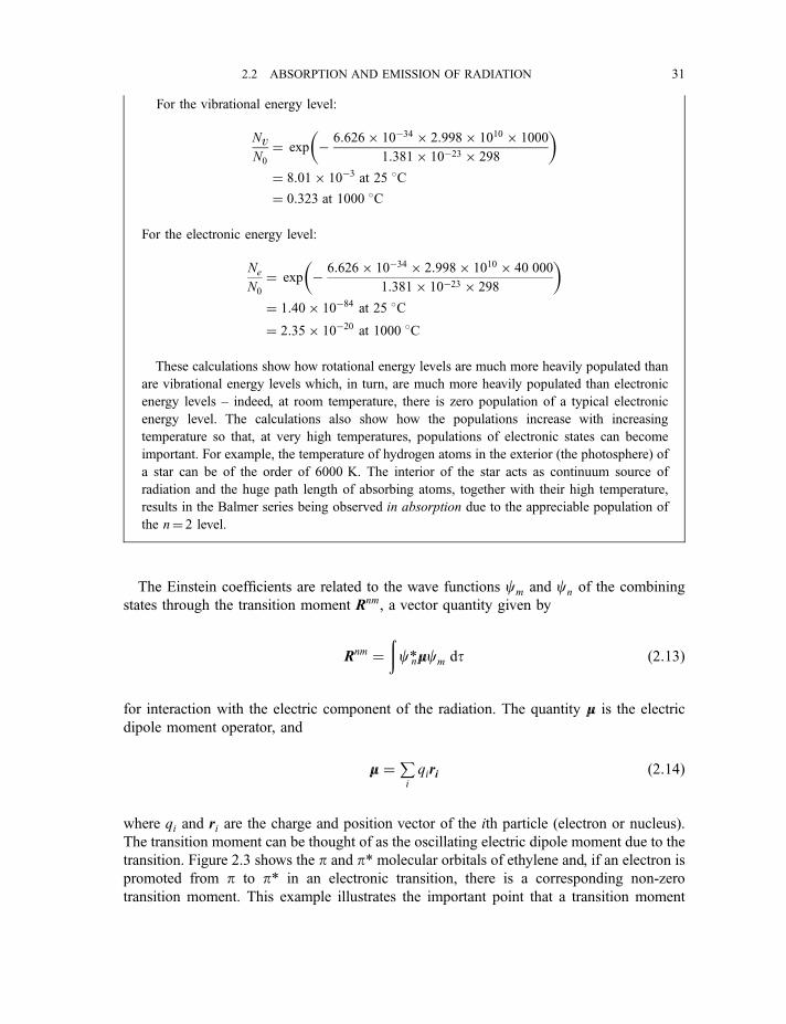
For the vibrational energy level:
NvN0
¼ exp � 6:626� 10�34 � 2:998� 1010 � 1000
1:381� 10�23 � 298
� �¼ 8:01� 10�3 at 25 �C¼ 0:323 at 1000 �C
For the electronic energy level:
Ne
N0
¼ exp � 6:626� 10�34 � 2:998� 1010 � 40 000
1:381� 10�23 � 298
� �¼ 1:40� 10�84 at 25 �C
¼ 2:35� 10�20 at 1000 �C
These calculations show how rotational energy levels are much more heavily populated than
are vibrational energy levels which, in turn, are much more heavily populated than electronic
energy levels – indeed, at room temperature, there is zero population of a typical electronic
energy level. The calculations also show how the populations increase with increasing
temperature so that, at very high temperatures, populations of electronic states can become
important. For example, the temperature of hydrogen atoms in the exterior (the photosphere) of
a star can be of the order of 6000 K. The interior of the star acts as continuum source of
radiation and the huge path length of absorbing atoms, together with their high temperature,
results in the Balmer series being observed in absorption due to the appreciable population of
the n¼ 2 level.
The Einstein coefficients are related to the wave functions cm and cn of the combining
states through the transition moment Rnm, a vector quantity given by
Rnm ¼ðc*nmmcm dt ð2:13Þ
for interaction with the electric component of the radiation. The quantity mm is the electric
dipole moment operator, and
mm ¼Pi
qiri ð2:14Þ
where qi and ri are the charge and position vector of the ith particle (electron or nucleus).
The transition moment can be thought of as the oscillating electric dipole moment due to the
transition. Figure 2.3 shows the p and p* molecular orbitals of ethylene and, if an electron is
promoted from p to p* in an electronic transition, there is a corresponding non-zero
transition moment. This example illustrates the important point that a transition moment
2.2 ABSORPTION AND EMISSION OF RADIATION 31
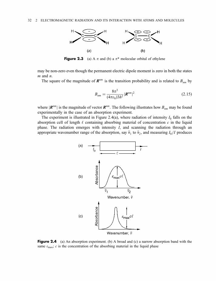
may be non-zero even though the permanent electric dipole moment is zero in both the states
m and n.
The square of the magnitude of Rnm is the transition probability and is related to Bnm by
Bnm ¼8p3
ð4pe0Þ3h2jRnmj2 ð2:15Þ
where jRnmj is the magnitude of vector Rnm: The following illustrates how Bnm may be found
experimentally in the case of an absorption experiment.
The experiment is illustrated in Figure 2.4(a), where radiation of intensity I0 falls on the
absorption cell of length ‘ containing absorbing material of concentration c in the liquid
phase. The radiation emerges with intensity I, and scanning the radiation through an
appropriate wavenumber range of the absorption, say ~nn1 to ~nn2, and measuring I0=I produces
Figure 2.3 (a) A p and (b) a p* molecular orbital of ethylene
Figure 2.4 (a) An absorption experiment. (b) A broad and (c) a narrow absorption band with the
same emax; c is the concentration of the absorbing material in the liquid phase
32 2 ELECTROMAGNETIC RADIATION AND ITS INTERACTION WITH ATOMS AND MOLECULES
the absorption spectrum typically measured as absorbance, defined as log10ðI0=I Þ.According to the Beer–Lambert law the absorbance A is proportional to c and ‘; so that
A ¼ log10I0
I
� �¼ eð~nnÞc‘ ð2:16Þ
where e is a function of ~nn and is the molar absorption coefficient or molar absorptivity
(it used to be known as the molar extinction coefficient, which will be encountered in
older texts). Since A is dimensionless, e has dimensions of (concentration6 length)71 and
the units are very often mol71 dm3 cm71. The spectrum is shown in Figure 2.4(b). The
quantity emax corresponds to the maximum value of A and is sometimes used as a measure of
the total absorption intensity. However, the spectrum in Figure 2.4(c), which has the same
emax but a much lower integrated intensity, illustrates the dangers of using emax. What we
should do is to integrate the area under the curve; then, provided Nn � Nm so that decay of
state n by induced emission is negligible,
ð ~nn2
~nn1
eð~nnÞd~nn ¼ NAh~nnnmBnm
ln 10ð2:17Þ
where ~nnnm is the average wavenumber of the absorption and NA is the Avogadro constant.
If the absorption is due to an electronic transition then fnm, the oscillator strength, is often
used to quantify the intensity and is related to the area under the curve by
fnm ¼4e0mec
2 ln 10
NAe2
ð ~nn2
~nn1
eð~nnÞd~nn ð2:18Þ
The quantity fnm is dimensionless and is the ratio of the strength of the transition to that of an
electric dipole transition between two states of an electron oscillating in three dimensions in
a simple harmonic way, and its maximum value is usually 1.
The transition probability jRnmj2 is related to selection rules in spectroscopy: it is zero for
a forbidden transition and non-zero for an allowed transition. By ‘forbidden’ or ‘allowed’ we
shall mostly be referring to electric dipole selection rules (i.e. to transitions occurring
through interaction with the electric vector of the radiation).
The electric dipole moment operator m has components along the cartesian axes:
mx ¼Pi
qixi; my ¼Pi
qiyi; mz ¼Pi
qizi ð2:19Þ
where qi and xi are, respectively, the charge and x coordinate of the ith particle, and so on.
Similarly, the transition moment can be resolved into three components such that
Rnmx ¼
ðc*nmxcm dx; Rnm
y ¼ðc*nmycm dy; Rnm
z ¼ðc*nmzcm dz ð2:20Þ
2.2 ABSORPTION AND EMISSION OF RADIATION 33
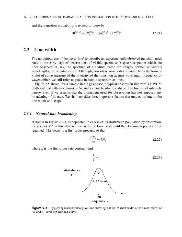
and the transition probability is related to these by
jRnmj2 ¼ ðRnmx Þ2 þ ðRnm
y Þ2 þ ðRnmz Þ2 ð2:21Þ
2.3 Line width
The ubiquitous use of the word ‘line’ to describe an experimentally observed transition goes
back to the early days of observations of visible spectra with spectroscopes in which the
lines observed in, say, the spectrum of a sodium flame are images, formed at various
wavelengths, of the entrance slit. Although, nowadays, observations tend to be in the form of
a plot of some measure of the intensity of the transition against wavelength, frequency or
wavenumber, we still refer to peaks in such a spectrum as lines.
Figure 2.5 shows, for a sample in the gas phase, a typical absorption line with a HWHM
(half-width at half-maximum) of Dn and a characteristic line shape. The line is not infinitely
narrow even if we assume that the instrument used for observation has not imposed any
broadening of its own. We shall consider three important factors that may contribute to the
line width and shape.
2.3.1 Natural line broadening
If state n in Figure 2.2(a) is populated in excess of its Boltzmann population by absorption,
the species M* in this state will decay to the lower state until the Boltzmann population is
regained. The decay is a first-order process, so that
� dNn
dt¼ kNn ð2:22Þ
where k is the first-order rate constant and
1
k¼ t ð2:23Þ
Figure 2.5 Typical (gaussian) absorption line showing a HWHM (half width at half maximum) of
Dn and a Lamb dip (dashed curve)
34 2 ELECTROMAGNETIC RADIATION AND ITS INTERACTION WITH ATOMS AND MOLECULES
Here, t is the time taken for Nn to fall to 1=e of its initial value (where e is the base of naturallogarithms) and is referred to as the lifetime of state n. If spontaneous emission is the only
process by which M* decays, comparison with Equation (2.9) shows that
k ¼ Anm ð2:24Þ
The Heisenberg uncertainty principle in the form
tDE 5 h ð2:25Þ
(see Equation 1.16) relates the lifetime to the smearing out, in terms of energy, of the state n.
This equation illustrates the point that state n has an exactly defined energy only if t is
infinite, but, since this is never the case, all energy levels are smeared out to some extent,
with resulting line broadening.
Combining Equations (2.12) and (2.15) relates Anm to the transition probability
Anm ¼64p4n3
ð4pe0Þ3hc3jRnmj2 ð2:26Þ
so that, from Equation (2.25),
Dn 532p3n3
ð4pe0Þ3hc3jRnmj2 ð2:27Þ
The dependence of Dn, the frequency spread, on n3 results in a much larger value for an
excited electronic state, typically 30 MHz, than for an excited rotational state, typically
1074–1075 Hz, because of the much greater n for an excited electronic state.
Equation (2.27) illustrates what is called the natural line broadening. Since each atom or
molecule behaves identically in this respect it is an example of homogeneous line
broadening, which results in a characteristic lorentzian line shape.
Natural line broadening is usually very small compared with other causes of broadening.
However, not only is it of considerable theoretical importance but also, in the ingenious
technique of Lamb dip spectroscopy (see Section 2.3.5.2), observations may be made of
spectra in which all other sources of broadening are removed.
2.3.2 Doppler broadening
Whether radiation is being absorbed or emitted the frequency at which it takes place
depends on the velocity of the atom or molecule relative to the detector. This is for the same
reason that an observer hears the whistle of a train travelling towards him or her as having a
frequency apparently higher than it really is, and lower when it is travelling away from him
or her. The effect is known as the Doppler effect.
2.3 LINE WIDTH 35
If an atom or molecule is travelling towards the detector with a velocity va, then the
frequency na at which a transition is observed to occur is related to the actual transition
frequency n in a stationary atom or molecule by
na ¼ n 1� vac
� ��1ð2:28Þ
where c is the speed of light. Because of the usual Maxwell velocity distribution there is a
spread of values of va and a characteristic line broadening given by
Dn ¼ nc
2kT ln 2
m
� �1=2
ð2:29Þ
where m is the mass of the atom or molecule; this Dn is normally far greater than the natural
line width. The broadening is inhomogeneous, since not all atoms or molecules in a
particular sample behave in the same way, and results in a line shape known as gaussian.
2.3.3 Pressure broadening
When collisions occur between gas phase atoms or molecules there is an exchange of
energy, which leads effectively to a broadening of energy levels. If t is the mean time
between collisions and each collision results in a transition between two states there is a line
broadening Dn of the transition, where
Dn ¼ ð2ptÞ�1 ð2:30Þ
derived from the uncertainty principle of Equation (1.16). This broadening is, like natural
line broadening, homogeneous and usually produces a lorentzian line shape except for
transitions at low frequencies, when an unsymmetrical line shape results.
2.3.4 Power, or saturation, broadening
The equilibrium populations of energy levels, given by the Boltzmann distribution law of
Equation 2.11, are maintained through exchange of energy by collisions. However, when the
ground and excited energy levels m and n, respectively, are close together the population
ratio Nn /Nm at equilibrium is close to 1. As a result, the equilibrium may be seriously
disturbed when, in obtaining an absorption spectrum, the molecular sample is subjected to
radiation of intensity I. As I is increased the limit of Nn /Nm ¼ 1 is approached, the Beer–
Lambert law (Equation 2.16) breaks down, e becomes dependent on I, and saturation is said
to occur. Clearly, this occurs more readily the closer the energy levels n and m.
Consequently, saturation is more common in microwave and millimetre wave spectroscopy,
36 2 ELECTROMAGNETIC RADIATION AND ITS INTERACTION WITH ATOMS AND MOLECULES
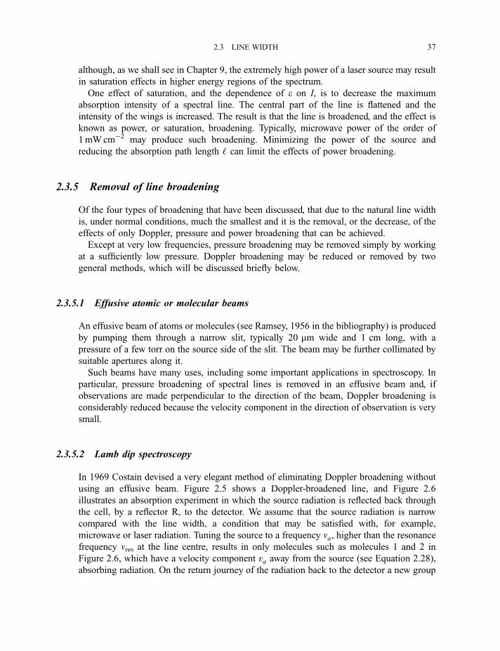
although, as we shall see in Chapter 9, the extremely high power of a laser source may result
in saturation effects in higher energy regions of the spectrum.
One effect of saturation, and the dependence of e on I, is to decrease the maximum
absorption intensity of a spectral line. The central part of the line is flattened and the
intensity of the wings is increased. The result is that the line is broadened, and the effect is
known as power, or saturation, broadening. Typically, microwave power of the order of
1mWcm�2 may produce such broadening. Minimizing the power of the source and
reducing the absorption path length ‘ can limit the effects of power broadening.
2.3.5 Removal of line broadening
Of the four types of broadening that have been discussed, that due to the natural line width
is, under normal conditions, much the smallest and it is the removal, or the decrease, of the
effects of only Doppler, pressure and power broadening that can be achieved.
Except at very low frequencies, pressure broadening may be removed simply by working
at a sufficiently low pressure. Doppler broadening may be reduced or removed by two
general methods, which will be discussed briefly below.
2.3.5.1 Effusive atomic or molecular beams
An effusive beam of atoms or molecules (see Ramsey, 1956 in the bibliography) is produced
by pumping them through a narrow slit, typically 20 mm wide and 1 cm long, with a
pressure of a few torr on the source side of the slit. The beam may be further collimated by
suitable apertures along it.
Such beams have many uses, including some important applications in spectroscopy. In
particular, pressure broadening of spectral lines is removed in an effusive beam and, if
observations are made perpendicular to the direction of the beam, Doppler broadening is
considerably reduced because the velocity component in the direction of observation is very
small.
2.3.5.2 Lamb dip spectroscopy
In 1969 Costain devised a very elegant method of eliminating Doppler broadening without
using an effusive beam. Figure 2.5 shows a Doppler-broadened line, and Figure 2.6
illustrates an absorption experiment in which the source radiation is reflected back through
the cell, by a reflector R, to the detector. We assume that the source radiation is narrow
compared with the line width, a condition that may be satisfied with, for example,
microwave or laser radiation. Tuning the source to a frequency na, higher than the resonance
frequency nres at the line centre, results in only molecules such as molecules 1 and 2 in
Figure 2.6, which have a velocity component va away from the source (see Equation 2.28),
absorbing radiation. On the return journey of the radiation back to the detector a new group
2.3 LINE WIDTH 37
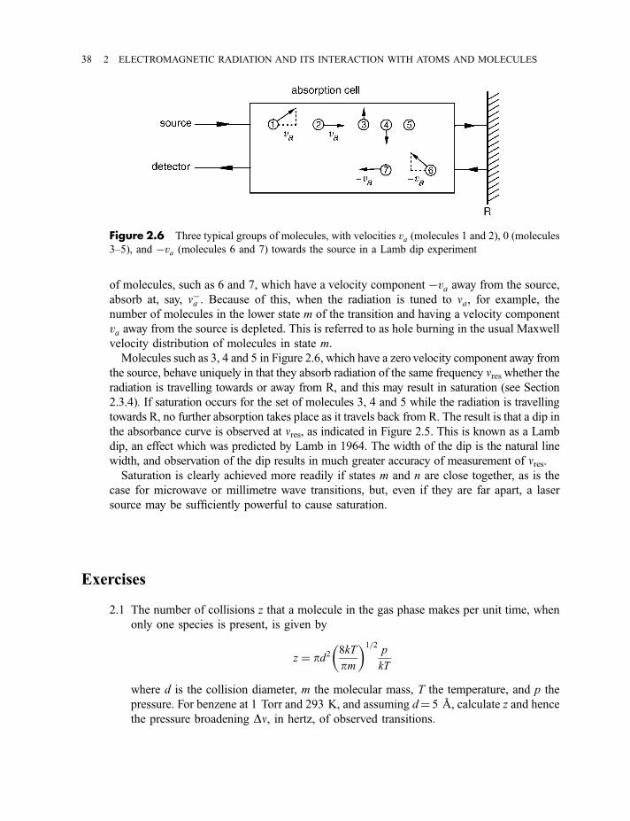
of molecules, such as 6 and 7, which have a velocity component �va away from the source,
absorb at, say, n�a . Because of this, when the radiation is tuned to na, for example, the
number of molecules in the lower state m of the transition and having a velocity component
va away from the source is depleted. This is referred to as hole burning in the usual Maxwell
velocity distribution of molecules in state m.
Molecules such as 3, 4 and 5 in Figure 2.6, which have a zero velocity component away from
the source, behave uniquely in that they absorb radiation of the same frequency nres whether theradiation is travelling towards or away from R, and this may result in saturation (see Section
2.3.4). If saturation occurs for the set of molecules 3, 4 and 5 while the radiation is travelling
towards R, no further absorption takes place as it travels back from R. The result is that a dip in
the absorbance curve is observed at nres, as indicated in Figure 2.5. This is known as a Lamb
dip, an effect which was predicted by Lamb in 1964. The width of the dip is the natural line
width, and observation of the dip results in much greater accuracy of measurement of nres.Saturation is clearly achieved more readily if states m and n are close together, as is the
case for microwave or millimetre wave transitions, but, even if they are far apart, a laser
source may be sufficiently powerful to cause saturation.
Exercises
2.1 The number of collisions z that a molecule in the gas phase makes per unit time, when
only one species is present, is given by
z ¼ pd28kT
pm
� �1=2p
kT
where d is the collision diameter, m the molecular mass, T the temperature, and p the
pressure. For benzene at 1 Torr and 293 K, and assuming d¼ 5 A, calculate z and hence
the pressure broadening Dn, in hertz, of observed transitions.
Figure 2.6 Three typical groups of molecules, with velocities va (molecules 1 and 2), 0 (molecules
3–5), and �va (molecules 6 and 7) towards the source in a Lamb dip experiment
38 2 ELECTROMAGNETIC RADIATION AND ITS INTERACTION WITH ATOMS AND MOLECULES
2.2 Calculate in hertz the broadening Dn of transitions in HCN at 25 �C due to the Doppler
effect in regions of the spectrum typical of rotational transitions (10 cm71), vibrational
transitions (1500 cm71) and electronic transitions (60 000 cm71).
2.3 As a function of frequency, the spectral radiation density is given by
rðnÞ ¼ 8phn3
c31
expðhn=kT Þ � 1
Calculate typical values in the microwave (n¼ 50 GHz) and near-ultraviolet
(~nn¼ 30 000 cm71) regions.
Bibliography
Ramsey, N. F. (1956) Molecular Beams, Oxford University Press, Oxford.
Townes, C. H. and Schawlow, A. L. (1955) Microwave Spectroscopy, McGraw-Hill, New York.
BIBLIOGRAPHY 39

3General Features of ExperimentalMethods
3.1 The electromagnetic spectrum
In a vacuum all electromagnetic radiation travels at the same speed, the speed of light c, and
may be characterized by its wavelength l, in air or vacuum, or by its wavenumber ~nn or
frequency n, both conventionally in a vacuum, where
lvac ¼c
n¼ 1
~nnð3:1Þ
Figure 3.1 illustrates the extent of the electromagnetic spectrum from low-energy radiowave
to high-energy g-ray radiation. The division into the various named regions does not imply
any fundamental differences but is useful to indicate that different experimental techniques
are used. Indications of region boundaries, which should not be regarded as clear cut, are
given in wavelength (mm, mm or nm), frequency (GHz) and wavenumber (cm71). In
addition, in the high-energy regions the energy is indicated in electron volts (eV) where
1 eV ¼ hcð8065:54 cm�1Þ ¼ hð2:417 99� 1014 s�1Þ ð3:2Þ
Also indicated in Figure 3.1 are the processes that may occur in an atom or molecule
exposed to the radiation. A molecule may undergo rotational, vibrational, electronic or
ionization processes, in order of increasing energy (typical ranges are indicated). A
molecule may also scatter light in a Raman process, and the light source for such an
experiment is usually in the visible or near-ultraviolet region (see, however, Section 5.3.1).
An atom may undergo only an electronic transition or ionization since it has no rotational or
vibrational degrees of freedom. Nuclear magnetic resonance (NMR) and electron spin
resonance (ESR) processes involve transitions between nuclear spin and electron spin states,
respectively, but these spectroscopies necessitate the sample being between the poles of a
magnet and will not be covered in this book.
41
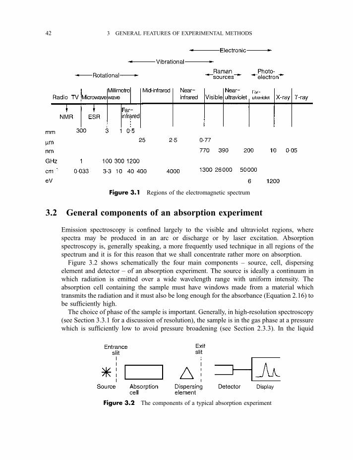
3.2 General components of an absorption experiment
Emission spectroscopy is confined largely to the visible and ultraviolet regions, where
spectra may be produced in an arc or discharge or by laser excitation. Absorption
spectroscopy is, generally speaking, a more frequently used technique in all regions of the
spectrum and it is for this reason that we shall concentrate rather more on absorption.
Figure 3.2 shows schematically the four main components – source, cell, dispersing
element and detector – of an absorption experiment. The source is ideally a continuum in
which radiation is emitted over a wide wavelength range with uniform intensity. The
absorption cell containing the sample must have windows made from a material which
transmits the radiation and it must also be long enough for the absorbance (Equation 2.16) to
be sufficiently high.
The choice of phase of the sample is important. Generally, in high-resolution spectroscopy
(see Section 3.3.1 for a discussion of resolution), the sample is in the gas phase at a pressure
which is sufficiently low to avoid pressure broadening (see Section 2.3.3). In the liquid
Figure 3.1 Regions of the electromagnetic spectrum
Figure 3.2 The components of a typical absorption experiment
42 3 GENERAL FEATURES OF EXPERIMENTAL METHODS
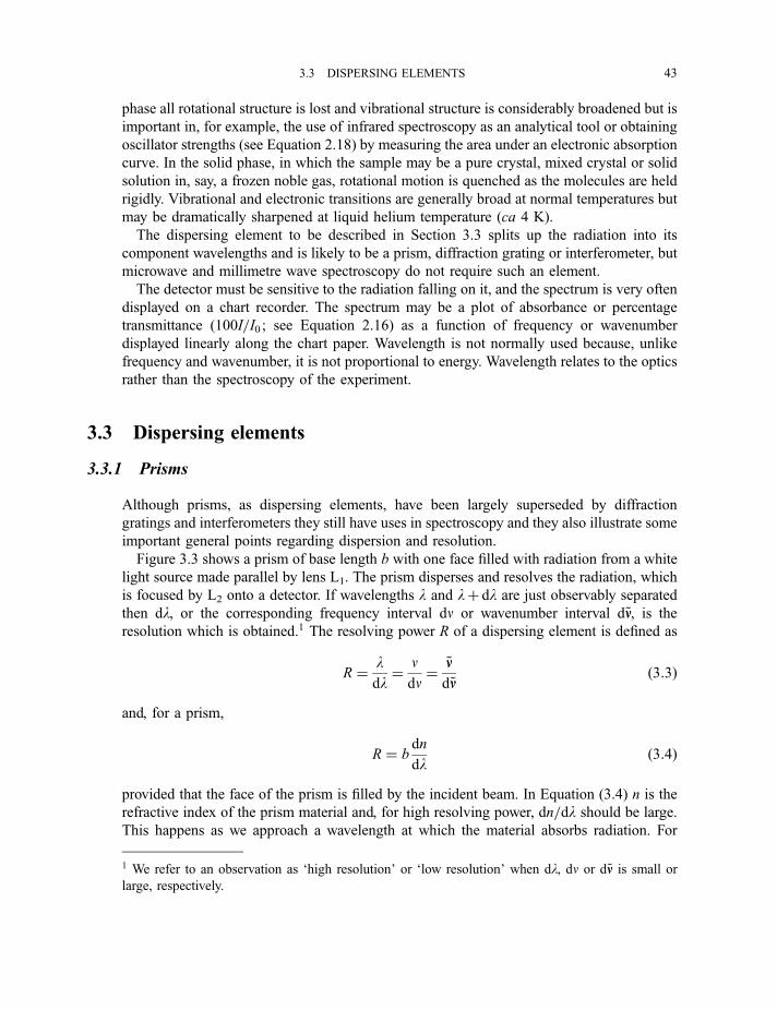
phase all rotational structure is lost and vibrational structure is considerably broadened but is
important in, for example, the use of infrared spectroscopy as an analytical tool or obtaining
oscillator strengths (see Equation 2.18) by measuring the area under an electronic absorption
curve. In the solid phase, in which the sample may be a pure crystal, mixed crystal or solid
solution in, say, a frozen noble gas, rotational motion is quenched as the molecules are held
rigidly. Vibrational and electronic transitions are generally broad at normal temperatures but
may be dramatically sharpened at liquid helium temperature (ca 4 K).
The dispersing element to be described in Section 3.3 splits up the radiation into its
component wavelengths and is likely to be a prism, diffraction grating or interferometer, but
microwave and millimetre wave spectroscopy do not require such an element.
The detector must be sensitive to the radiation falling on it, and the spectrum is very often
displayed on a chart recorder. The spectrum may be a plot of absorbance or percentage
transmittance (100I=I0; see Equation 2.16) as a function of frequency or wavenumber
displayed linearly along the chart paper. Wavelength is not normally used because, unlike
frequency and wavenumber, it is not proportional to energy. Wavelength relates to the optics
rather than the spectroscopy of the experiment.
3.3 Dispersing elements
3.3.1 Prisms
Although prisms, as dispersing elements, have been largely superseded by diffraction
gratings and interferometers they still have uses in spectroscopy and they also illustrate some
important general points regarding dispersion and resolution.
Figure 3.3 shows a prism of base length b with one face filled with radiation from a white
light source made parallel by lens L1. The prism disperses and resolves the radiation, which
is focused by L2 onto a detector. If wavelengths l and lþ dl are just observably separated
then dl, or the corresponding frequency interval dn or wavenumber interval d~nn, is the
resolution which is obtained.1 The resolving power R of a dispersing element is defined as
R ¼ ldl¼ n
dn¼ ~nn
d~nnð3:3Þ
and, for a prism,
R ¼ bdn
dlð3:4Þ
provided that the face of the prism is filled by the incident beam. In Equation (3.4) n is the
refractive index of the prism material and, for high resolving power, dn=dl should be large.
This happens as we approach a wavelength at which the material absorbs radiation. For
1 We refer to an observation as ‘high resolution’ or ‘low resolution’ when dl, dn or d~nn is small or
large, respectively.
3.3 DISPERSING ELEMENTS 43
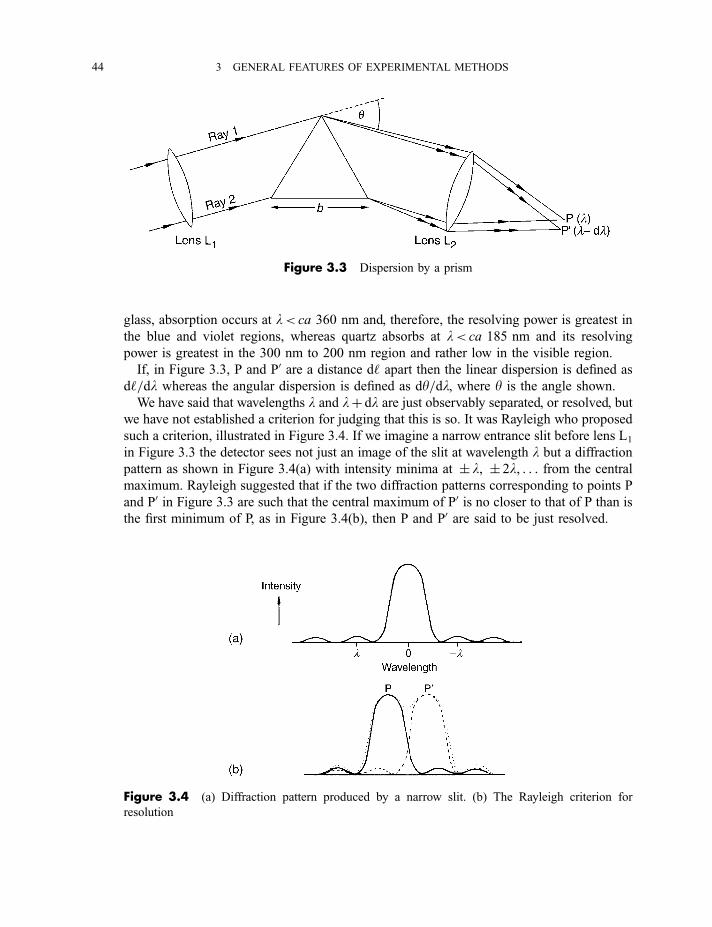
glass, absorption occurs at l< ca 360 nm and, therefore, the resolving power is greatest in
the blue and violet regions, whereas quartz absorbs at l< ca 185 nm and its resolving
power is greatest in the 300 nm to 200 nm region and rather low in the visible region.
If, in Figure 3.3, P and P0 are a distance d‘ apart then the linear dispersion is defined as
d‘=dl whereas the angular dispersion is defined as dy=dl, where y is the angle shown.
We have said that wavelengths l and lþ dl are just observably separated, or resolved, but
we have not established a criterion for judging that this is so. It was Rayleigh who proposed
such a criterion, illustrated in Figure 3.4. If we imagine a narrow entrance slit before lens L1
in Figure 3.3 the detector sees not just an image of the slit at wavelength l but a diffraction
pattern as shown in Figure 3.4(a) with intensity minima at � l, � 2l, . . . from the central
maximum. Rayleigh suggested that if the two diffraction patterns corresponding to points P
and P0 in Figure 3.3 are such that the central maximum of P0 is no closer to that of P than is
the first minimum of P, as in Figure 3.4(b), then P and P0 are said to be just resolved.
Figure 3.4 (a) Diffraction pattern produced by a narrow slit. (b) The Rayleigh criterion for
resolution
Figure 3.3 Dispersion by a prism
44 3 GENERAL FEATURES OF EXPERIMENTAL METHODS
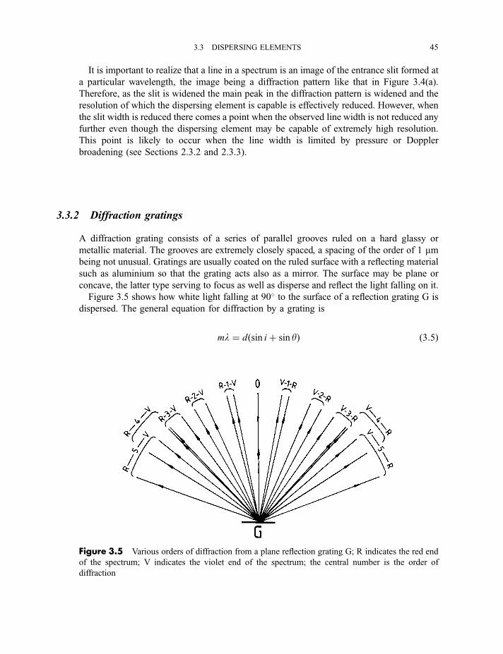
It is important to realize that a line in a spectrum is an image of the entrance slit formed at
a particular wavelength, the image being a diffraction pattern like that in Figure 3.4(a).
Therefore, as the slit is widened the main peak in the diffraction pattern is widened and the
resolution of which the dispersing element is capable is effectively reduced. However, when
the slit width is reduced there comes a point when the observed line width is not reduced any
further even though the dispersing element may be capable of extremely high resolution.
This point is likely to occur when the line width is limited by pressure or Doppler
broadening (see Sections 2.3.2 and 2.3.3).
3.3.2 Diffraction gratings
A diffraction grating consists of a series of parallel grooves ruled on a hard glassy or
metallic material. The grooves are extremely closely spaced, a spacing of the order of 1 mmbeing not unusual. Gratings are usually coated on the ruled surface with a reflecting material
such as aluminium so that the grating acts also as a mirror. The surface may be plane or
concave, the latter type serving to focus as well as disperse and reflect the light falling on it.
Figure 3.5 shows how white light falling at 90� to the surface of a reflection grating G is
dispersed. The general equation for diffraction by a grating is
ml ¼ dðsin iþ sin yÞ ð3:5Þ
Figure 3.5 Various orders of diffraction from a plane reflection grating G; R indicates the red end
of the spectrum; V indicates the violet end of the spectrum; the central number is the order of
diffraction
3.3 DISPERSING ELEMENTS 45
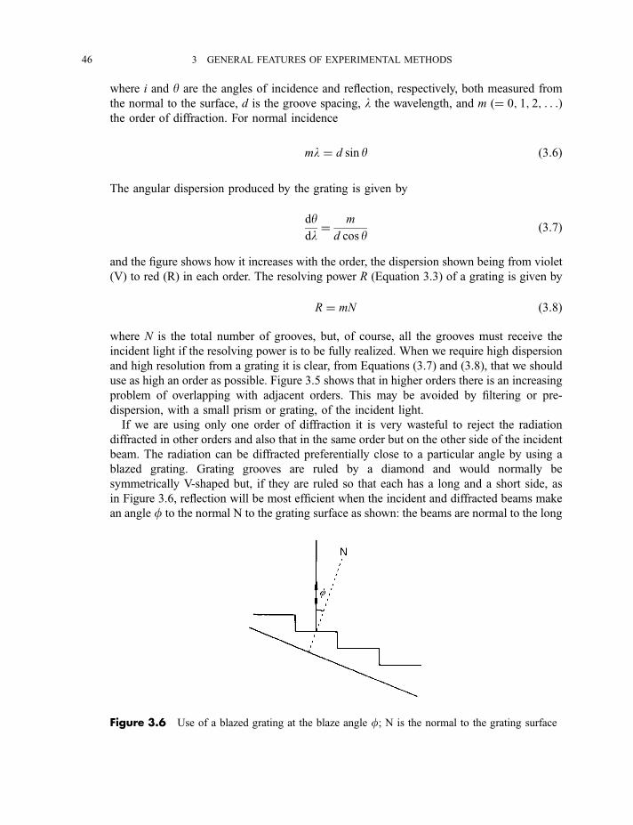
where i and y are the angles of incidence and reflection, respectively, both measured from
the normal to the surface, d is the groove spacing, l the wavelength, and m (¼ 0; 1; 2; . . .)the order of diffraction. For normal incidence
ml ¼ d sin y ð3:6Þ
The angular dispersion produced by the grating is given by
dydl¼ m
d cos yð3:7Þ
and the figure shows how it increases with the order, the dispersion shown being from violet
(V) to red (R) in each order. The resolving power R (Equation 3.3) of a grating is given by
R ¼ mN ð3:8Þ
where N is the total number of grooves, but, of course, all the grooves must receive the
incident light if the resolving power is to be fully realized. When we require high dispersion
and high resolution from a grating it is clear, from Equations (3.7) and (3.8), that we should
use as high an order as possible. Figure 3.5 shows that in higher orders there is an increasing
problem of overlapping with adjacent orders. This may be avoided by filtering or pre-
dispersion, with a small prism or grating, of the incident light.
If we are using only one order of diffraction it is very wasteful to reject the radiation
diffracted in other orders and also that in the same order but on the other side of the incident
beam. The radiation can be diffracted preferentially close to a particular angle by using a
blazed grating. Grating grooves are ruled by a diamond and would normally be
symmetrically V-shaped but, if they are ruled so that each has a long and a short side, as
in Figure 3.6, reflection will be most efficient when the incident and diffracted beams make
an angle f to the normal N to the grating surface as shown: the beams are normal to the long
Figure 3.6 Use of a blazed grating at the blaze angle f; N is the normal to the grating surface
46 3 GENERAL FEATURES OF EXPERIMENTAL METHODS
side of the groove. The angle f is called the blaze angle, and when the grating is used with
equal angles of incidence and reflection, as in the figure, Equation (3.5) becomes
ml ¼ 2d sin y ð3:9Þ
Diffraction gratings may be made by a holographic process, but blaze characteristics
cannot be controlled and their efficiency is low in the infrared. They are mostly used for low-
order work in the visible and near-ultraviolet.
Worked example 3.1
Question. A diffraction grating has a ruled area that is 10.40 cm wide, has 600.0 grooves per
millimetre and is blazed at an angle of 45.00�.(a) What is the wavelength of radiation diffracted at the blaze angle in the first, fourth and ninth
orders?
(b) What is the resolving power in these orders?
(c) What is the resolution in terms of wavelength (nm), wavenumber (cm71) and frequency
(GHz) in the ninth order at 300 nm?
Answer.
(a) The grating is 104.0 mm wide. Thus the total number of grooves is given by
N ¼ 104:0 mm� 600:0 mm�1 ¼ 62 400
and the spacing between grooves by
d ¼ 0:1040 m
62 400
¼ 1:6667� 10�6 m
¼ 1666:7 nm
The Bragg equation for diffraction is given by Equation (3.9):
ml ¼ 2d sin y
¼ 2� 1666:7 nm� 0:70711
¼ 2357:1 nm
; l ¼2357 nm for m ¼ 1
589:3 nm for m ¼ 4
261:9 nm for m ¼ 9
8><>:
3.3 DISPERSING ELEMENTS 47
(b) The resolving power R of the grating is given by Equation (3.8) as
R ¼ mN
¼ 62 400m
; R ¼62 400 for m ¼ 1
249 600 for m ¼ 4
561 600 for m ¼ 9
8><>:
(c) The resolution dl, d~nn or dn is obtained from the resolving power by using Equation (3.3)
R ¼ ldl¼ ~nn
d~nn¼ ndn
; dl ¼ lR¼ 300:0 nm
561 600
¼5:342� 10�4 nm
For l¼ 300.0 nm,
~nn ¼ 1
l¼ 1
300:0 nm¼ 1
300:0� 10�7 cm¼ 33 333 cm�1
; d~nn ¼ ~nnR¼ 33 333 cm�1
561 600
¼ 0:05935 cm�1
For l¼ 300.0 nm,
n ¼ c
l¼ 2:998� 1010 cm s�1
300:0� 10�7 cm¼ 9:9933� 1014 s�1
¼ 9:9933� 105 GHz
; dn ¼ nR¼ 9:9933� 105 GHz
561 600
¼ 1:779 GHz
3.3.3 Fourier transformation and interferometers
A thin layer of oil on water often shows regions of different colours, and this illustrates a
third method of dispersing light. White light falling on the oil is reflected backwards and
forwards within the layer, a part of the beam emerging from the surface each time. The
various emerging beams may interfere constructively or destructively with each other,
depending on the wavelength, and give rise to the different colours observed. This principle
is made use of in an interferometer, which is used to disperse infrared, visible or ultraviolet
radiation but is especially important for infrared radiation.
48 3 GENERAL FEATURES OF EXPERIMENTAL METHODS
We shall discuss infrared interferometers in Section 3.3.3.2 but, before this, we need to
understand the principles of Fourier transformation since this is involved in the very
important step in treating the signal from an interferometer. This signal does not resemble
the kind of spectrum that we usually obtain from a spectrometer and it is the modification of
the signal to the intensity-versus-wavelength type of spectrum which we require that
involves Fourier transformation. The principles of Fourier transformation are probably easier
to understand when applied to longer wavelength radiofrequency radiation than to shorter
wavelength infrared, visible or ultraviolet radiation. We shall consider radiofrequency
radiation first.
3.3.3.1 Radiofrequency radiation
Consider radiofrequency radiation with a frequency of 100 MHz, or a wavelength of 3 m.
Such radiation is used, for example, in a nuclear magnetic resonance (NMR) spectrometer
and as a carrier of FM (or VHF) radio signals. Frequencies typical of radiofrequency
radiation are relatively low compared with, say, near-infrared radiation of frequency
10 000 GHz (see Figure 3.1). Consequently there is no problem in producing detectors that
can respond sufficiently rapidly to determine the frequency of a radiofrequency signal
directly. If we consider a source of monochromatic radiofrequency radiation, the detector
responds to the electric field E which is oscillating, as in Figure 2.1, at a frequency n. Thevariation of the signal detected, f (t), with time t is shown in Figure 3.7(a) and is said to be
the spectrum in the time domain. In this case it is the spectrum of a monochromatic source.
We are more used to spectra recorded not in the time domain but in the frequency (or
wavenumber or wavelength) domain in which the detector signal is plotted against, say,
frequency n rather than time t. We can easily see that the time domain spectrum in Figure
3.7(a) corresponds to the frequency domain spectrum in Figure 3.7(b) in which the signal
F(n) is plotted against frequency. The monochromatic source produces a single line
spectrum.
The process of going from the time domain spectrum f (t) to the frequency domain
spectrum F(n) is known as Fourier transformation. In this case the frequency of the line, say
100 MHz, in Figure 3.7(b) is simply the value of n which appears in the equation
f ðtÞ ¼ A cos 2pnt ð3:10Þ
for the time domain spectrum, where A is the amplitude of f ðtÞ.If the source emits radiofrequency radiation consisting of two frequencies, n and 1
4n, of the
same amplitude then
f ðtÞ ¼ A½cos 2pnt þ cos 2pð14nÞt� ð3:11Þ
and this is shown in Figure 3.8(a). The corresponding frequency domain spectrum is
illustrated in Figure 3.8(b), which shows two equally intense lines, one at 100 MHz and the
other at 25 MHz.
3.3 DISPERSING ELEMENTS 49
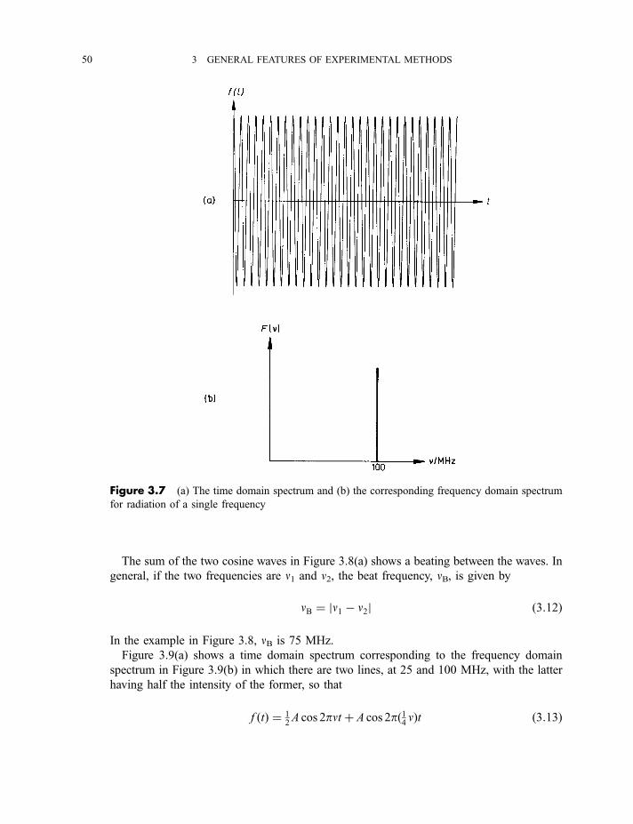
The sum of the two cosine waves in Figure 3.8(a) shows a beating between the waves. In
general, if the two frequencies are n1 and n2, the beat frequency, nB, is given by
nB ¼ jn1 � n2j ð3:12Þ
In the example in Figure 3.8, nB is 75 MHz.
Figure 3.9(a) shows a time domain spectrum corresponding to the frequency domain
spectrum in Figure 3.9(b) in which there are two lines, at 25 and 100 MHz, with the latter
having half the intensity of the former, so that
f ðtÞ ¼ 12A cos 2pnt þ A cos 2pð1
4nÞt ð3:13Þ
Figure 3.7 (a) The time domain spectrum and (b) the corresponding frequency domain spectrum
for radiation of a single frequency
50 3 GENERAL FEATURES OF EXPERIMENTAL METHODS
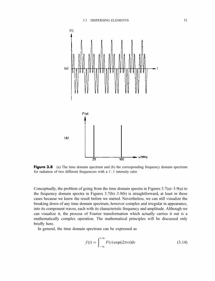
Conceptually, the problem of going from the time domain spectra in Figures 3.7(a)–3.9(a) to
the frequency domain spectra in Figures 3.7(b)–3.9(b) is straightforward, at least in these
cases because we knew the result before we started. Nevertheless, we can still visualize the
breaking down of any time domain spectrum, however complex and irregular in appearance,
into its component waves, each with its characteristic frequency and amplitude. Although we
can visualize it, the process of Fourier transformation which actually carries it out is a
mathematically complex operation. The mathematical principles will be discussed only
briefly here.
In general, the time domain spectrum can be expressed as
f ðtÞ ¼ðþ1�1
FðnÞ expði2pntÞdn ð3:14Þ
Figure 3.8 (a) The time domain spectrum and (b) the corresponding frequency domain spectrum
for radiation of two different frequencies with a 1 : 1 intensity ratio
3.3 DISPERSING ELEMENTS 51
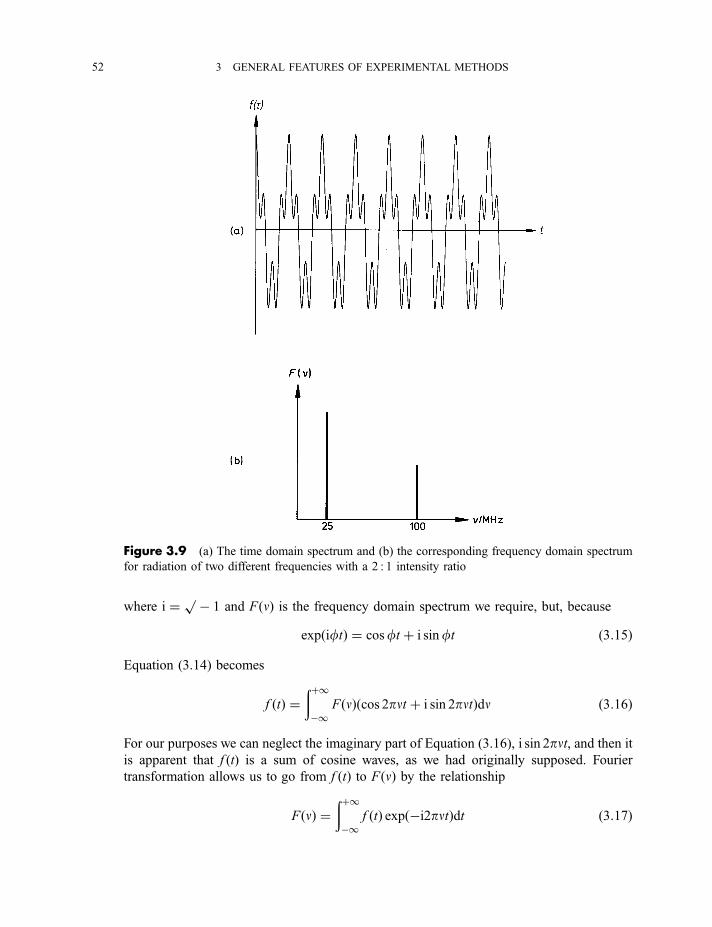
where i ¼ p � 1 and FðnÞ is the frequency domain spectrum we require, but, because
expðiftÞ ¼ cosft þ i sinft ð3:15Þ
Equation (3.14) becomes
f ðtÞ ¼ðþ1�1
FðnÞðcos 2pnt þ i sin 2pntÞdn ð3:16Þ
For our purposes we can neglect the imaginary part of Equation (3.16), i sin 2pnt, and then itis apparent that f (t) is a sum of cosine waves, as we had originally supposed. Fourier
transformation allows us to go from f ðtÞ to FðnÞ by the relationship
FðnÞ ¼ðþ1�1
f ðtÞ expð�i2pntÞdt ð3:17Þ
Figure 3.9 (a) The time domain spectrum and (b) the corresponding frequency domain spectrum
for radiation of two different frequencies with a 2 : 1 intensity ratio
52 3 GENERAL FEATURES OF EXPERIMENTAL METHODS
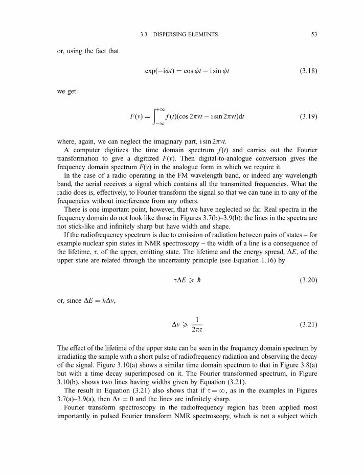
or, using the fact that
expð�iftÞ ¼ cosft � i sinft ð3:18Þ
we get
FðnÞ ¼ðþ1�1
f ðtÞðcos 2pnt � i sin 2pntÞdt ð3:19Þ
where, again, we can neglect the imaginary part, i sin 2pnt.A computer digitizes the time domain spectrum f (t) and carries out the Fourier
transformation to give a digitized F(n). Then digital-to-analogue conversion gives the
frequency domain spectrum F(n) in the analogue form in which we require it.
In the case of a radio operating in the FM wavelength band, or indeed any wavelength
band, the aerial receives a signal which contains all the transmitted frequencies. What the
radio does is, effectively, to Fourier transform the signal so that we can tune in to any of the
frequencies without interference from any others.
There is one important point, however, that we have neglected so far. Real spectra in the
frequency domain do not look like those in Figures 3.7(b)–3.9(b): the lines in the spectra are
not stick-like and infinitely sharp but have width and shape.
If the radiofrequency spectrum is due to emission of radiation between pairs of states – for
example nuclear spin states in NMR spectroscopy – the width of a line is a consequence of
the lifetime, t, of the upper, emitting state. The lifetime and the energy spread, DE, of theupper state are related through the uncertainty principle (see Equation 1.16) by
tDE 5 h ð3:20Þ
or, since DE ¼ hDn,
Dn 51
2ptð3:21Þ
The effect of the lifetime of the upper state can be seen in the frequency domain spectrum by
irradiating the sample with a short pulse of radiofrequency radiation and observing the decay
of the signal. Figure 3.10(a) shows a similar time domain spectrum to that in Figure 3.8(a)
but with a time decay superimposed on it. The Fourier transformed spectrum, in Figure
3.10(b), shows two lines having widths given by Equation (3.21).
The result in Equation (3.21) also shows that if t¼?, as in the examples in Figures
3.7(a)–3.9(a), then Dn ¼ 0 and the lines are infinitely sharp.
Fourier transform spectroscopy in the radiofrequency region has been applied most
importantly in pulsed Fourier transform NMR spectroscopy, which is not a subject which
3.3 DISPERSING ELEMENTS 53
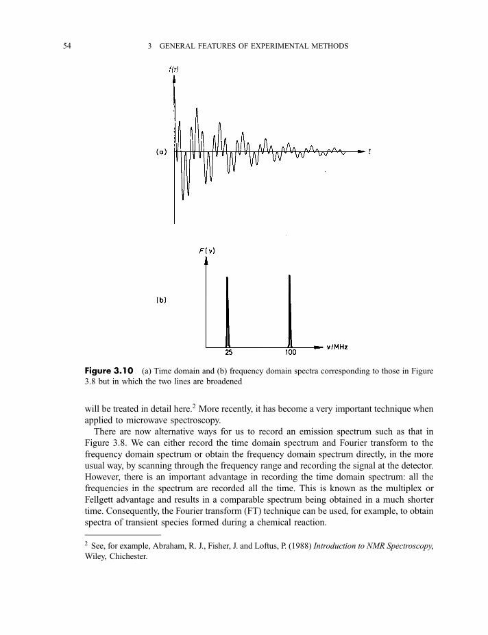
will be treated in detail here.2 More recently, it has become a very important technique when
applied to microwave spectroscopy.
There are now alternative ways for us to record an emission spectrum such as that in
Figure 3.8. We can either record the time domain spectrum and Fourier transform to the
frequency domain spectrum or obtain the frequency domain spectrum directly, in the more
usual way, by scanning through the frequency range and recording the signal at the detector.
However, there is an important advantage in recording the time domain spectrum: all the
frequencies in the spectrum are recorded all the time. This is known as the multiplex or
Fellgett advantage and results in a comparable spectrum being obtained in a much shorter
time. Consequently, the Fourier transform (FT) technique can be used, for example, to obtain
spectra of transient species formed during a chemical reaction.
Figure 3.10 (a) Time domain and (b) frequency domain spectra corresponding to those in Figure
3.8 but in which the two lines are broadened
2 See, for example, Abraham, R. J., Fisher, J. and Loftus, P. (1988) Introduction to NMR Spectroscopy,
Wiley, Chichester.
54 3 GENERAL FEATURES OF EXPERIMENTAL METHODS
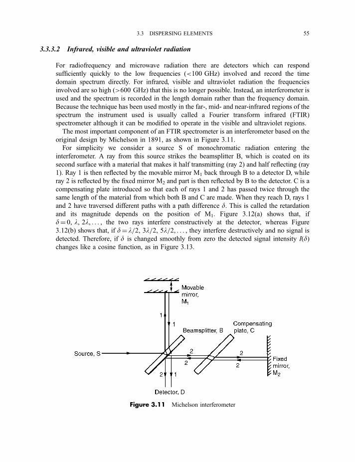
3.3.3.2 Infrared, visible and ultraviolet radiation
For radiofrequency and microwave radiation there are detectors which can respond
sufficiently quickly to the low frequencies (<100 GHz) involved and record the time
domain spectrum directly. For infrared, visible and ultraviolet radiation the frequencies
involved are so high (>600 GHz) that this is no longer possible. Instead, an interferometer is
used and the spectrum is recorded in the length domain rather than the frequency domain.
Because the technique has been used mostly in the far-, mid- and near-infrared regions of the
spectrum the instrument used is usually called a Fourier transform infrared (FTIR)
spectrometer although it can be modified to operate in the visible and ultraviolet regions.
The most important component of an FTIR spectrometer is an interferometer based on the
original design by Michelson in 1891, as shown in Figure 3.11.
For simplicity we consider a source S of monochromatic radiation entering the
interferometer. A ray from this source strikes the beamsplitter B, which is coated on its
second surface with a material that makes it half transmitting (ray 2) and half reflecting (ray
1). Ray 1 is then reflected by the movable mirror M1 back through B to a detector D, while
ray 2 is reflected by the fixed mirror M2 and part is then reflected by B to the detector. C is a
compensating plate introduced so that each of rays 1 and 2 has passed twice through the
same length of the material from which both B and C are made. When they reach D, rays 1
and 2 have traversed different paths with a path difference d. This is called the retardation
and its magnitude depends on the position of M1. Figure 3.12(a) shows that, if
d¼ 0, l, 2l, . . . , the two rays interfere constructively at the detector, whereas Figure
3.12(b) shows that, if d¼ l=2, 3l=2, 5l=2, . . . , they interfere destructively and no signal is
detected. Therefore, if d is changed smoothly from zero the detected signal intensity I(d)changes like a cosine function, as in Figure 3.13.
Figure 3.11 Michelson interferometer
3.3 DISPERSING ELEMENTS 55
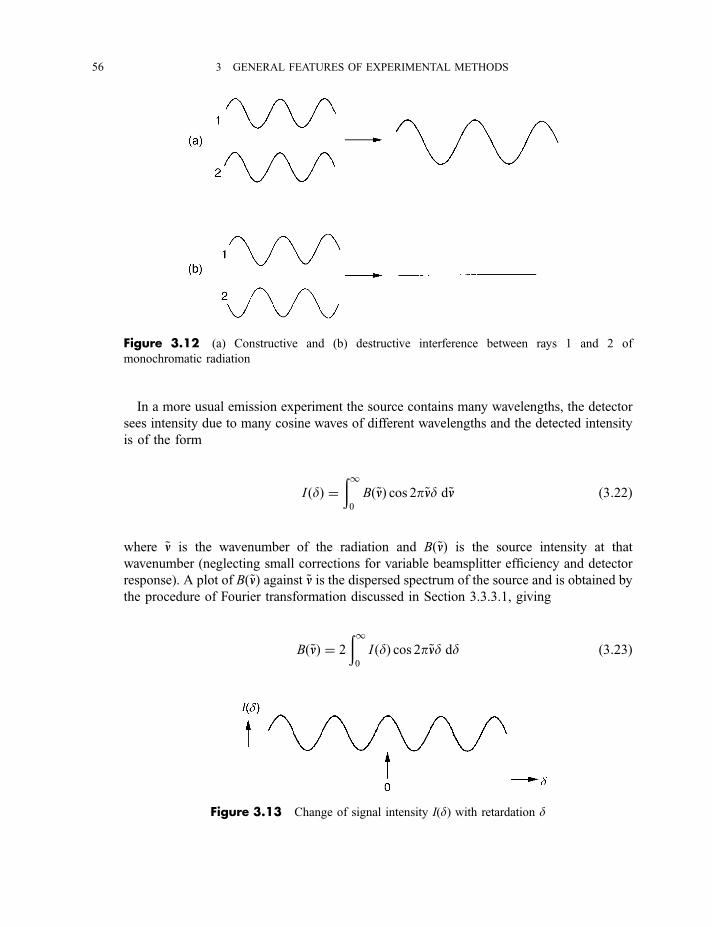
In a more usual emission experiment the source contains many wavelengths, the detector
sees intensity due to many cosine waves of different wavelengths and the detected intensity
is of the form
I ðdÞ ¼ð10
Bð~nnÞ cos 2p~nnd d~nn ð3:22Þ
where ~nn is the wavenumber of the radiation and Bð~nnÞ is the source intensity at that
wavenumber (neglecting small corrections for variable beamsplitter efficiency and detector
response). A plot of Bð~nnÞ against ~nn is the dispersed spectrum of the source and is obtained by
the procedure of Fourier transformation discussed in Section 3.3.3.1, giving
Bð~nnÞ ¼ 2
ð10
I ðdÞ cos 2p~nnd dd ð3:23Þ
Figure 3.12 (a) Constructive and (b) destructive interference between rays 1 and 2 of
monochromatic radiation
Figure 3.13 Change of signal intensity I(d) with retardation d
56 3 GENERAL FEATURES OF EXPERIMENTAL METHODS
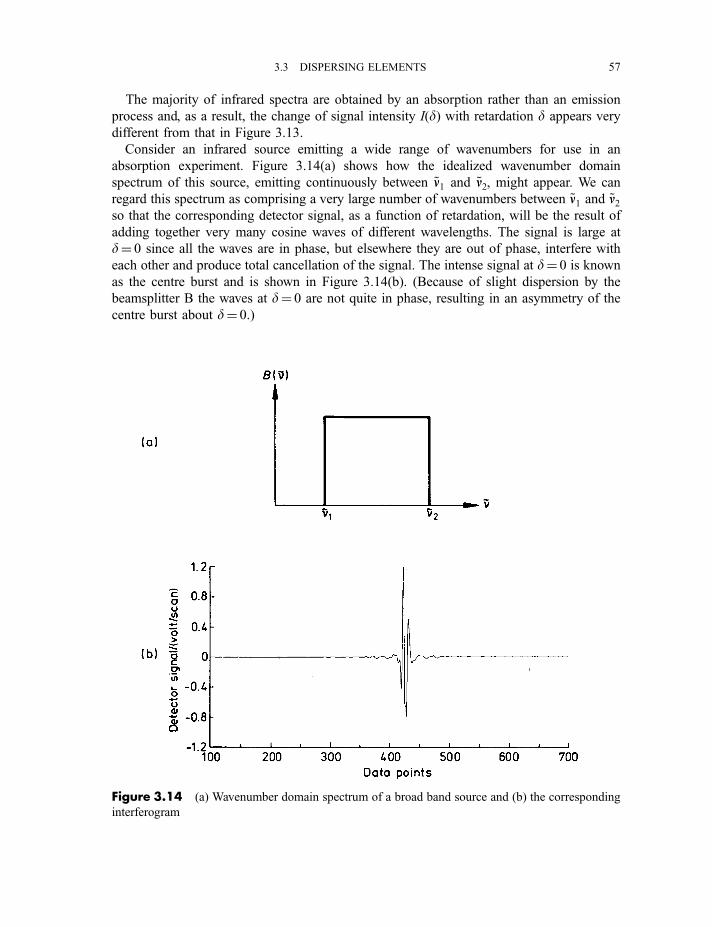
The majority of infrared spectra are obtained by an absorption rather than an emission
process and, as a result, the change of signal intensity I(d) with retardation d appears very
different from that in Figure 3.13.
Consider an infrared source emitting a wide range of wavenumbers for use in an
absorption experiment. Figure 3.14(a) shows how the idealized wavenumber domain
spectrum of this source, emitting continuously between ~nn1 and ~nn2, might appear. We can
regard this spectrum as comprising a very large number of wavenumbers between ~nn1 and ~nn2so that the corresponding detector signal, as a function of retardation, will be the result of
adding together very many cosine waves of different wavelengths. The signal is large at
d¼ 0 since all the waves are in phase, but elsewhere they are out of phase, interfere with
each other and produce total cancellation of the signal. The intense signal at d¼ 0 is known
as the centre burst and is shown in Figure 3.14(b). (Because of slight dispersion by the
beamsplitter B the waves at d¼ 0 are not quite in phase, resulting in an asymmetry of the
centre burst about d¼ 0.)
Figure 3.14 (a) Wavenumber domain spectrum of a broad band source and (b) the corresponding
interferogram
3.3 DISPERSING ELEMENTS 57
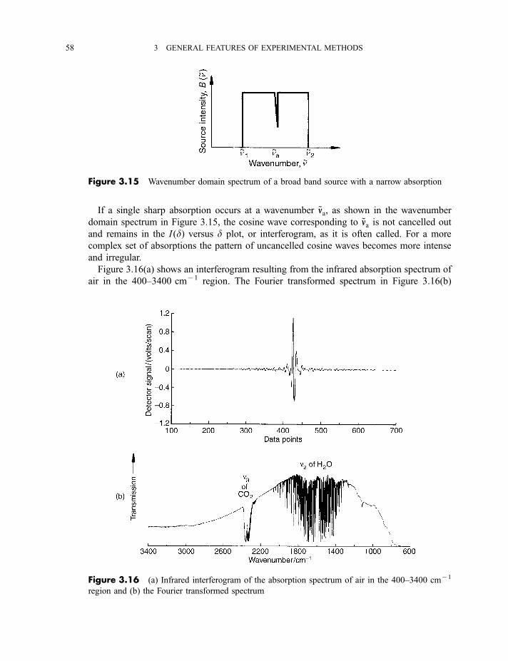
If a single sharp absorption occurs at a wavenumber ~nna, as shown in the wavenumber
domain spectrum in Figure 3.15, the cosine wave corresponding to ~nna is not cancelled out
and remains in the I ðdÞ versus d plot, or interferogram, as it is often called. For a more
complex set of absorptions the pattern of uncancelled cosine waves becomes more intense
and irregular.
Figure 3.16(a) shows an interferogram resulting from the infrared absorption spectrum of
air in the 400–3400 cm71 region. The Fourier transformed spectrum in Figure 3.16(b)
Figure 3.15 Wavenumber domain spectrum of a broad band source with a narrow absorption
Figure 3.16 (a) Infrared interferogram of the absorption spectrum of air in the 400–3400 cm71
region and (b) the Fourier transformed spectrum
58 3 GENERAL FEATURES OF EXPERIMENTAL METHODS
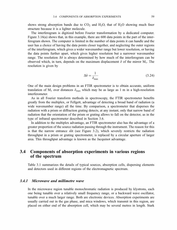
shows strong absorption bands due to CO2 and H2O, that of H2O showing much finer
structure because it is a lighter molecule.
The interferogram is digitized before Fourier transformation by a dedicated computer.
Figure 3.16(a) shows that, in this example, there are 600 data points in the part of the inter-
ferogram shown. The computer is limited in the number of data points it can handle and the
user has a choice of having the data points closer together, and neglecting the outer regions
of the interferogram, which gives a wider wavenumber range but lower resolution, or having
the data points further apart, which gives higher resolution but a narrower wavenumber
range. The resolution D~nn is always determined by how much of the interferogram can be
observed which, in turn, depends on the maximum displacement d of the mirror M1. The
resolution is given by
D~nn ¼ 1
dmax
ð3:24Þ
One of the main design problems in an FTIR spectrometer is to obtain accurate, uniform
translation of M1 over distances dmax which may be as large as 1 m in a high-resolution
interferometer.
As in all Fourier transform methods in spectroscopy, the FTIR spectrometer benefits
greatly from the multiplex, or Fellgett, advantage of detecting a broad band of radiation (a
wide wavenumber range) all the time. By comparison, a spectrometer that disperses the
radiation with a prism or diffraction grating detects, at any instant, only that narrow band of
radiation that the orientation of the prism or grating allows to fall on the detector, as in the
type of infrared spectrometer described in Section 3.6.
In addition to the multiplex advantage, an FTIR spectrometer also has the advantage of a
greater proportion of the source radiation passing through the instrument. The reason for this
is that the narrow entrance slit (see Figure 3.2), which severely restricts the radiation
throughput in a prism or grating spectrometer, is replaced by a circular aperture of larger
area. This throughput advantage is known as the Jacquinot advantage.
3.4 Components of absorption experiments in various regionsof the spectrum
Table 3.1 summarizes the details of typical sources, absorption cells, dispersing elements
and detectors used in different regions of the electromagnetic spectrum.
3.4.1 Microwave and millimetre wave
In the microwave region tunable monochromatic radiation is produced by klystrons, each
one being tunable over a relatively small frequency range, or a backward wave oscillator,
tunable over a much larger range. Both are electronic devices. Absorption experiments are
usually carried out in the gas phase, and mica windows, which transmit in this region, are
placed on either end of the absorption cell, which may be several metres in length. Stark
3.4 COMPONENTS OF ABSORPTION EXPERIMENTS 59
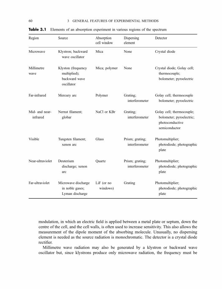
modulation, in which an electric field is applied between a metal plate or septum, down the
centre of the cell, and the cell walls, is often used to increase sensitivity. This also allows the
measurement of the dipole moment of the absorbing molecule. Unusually, no dispersing
element is needed as the source radiation is monochromatic. The detector is a crystal diode
rectifier.
Millimetre wave radiation may also be generated by a klystron or backward wave
oscillator but, since klystrons produce only microwave radiation, the frequency must be
Table 3.1 Elements of an absorption experiment in various regions of the spectrum
Region Source Absorption
cell window
Dispersing
element
Detector
Microwave Klystron; backward
wave oscillator
Mica None Crystal diode
Millimetre
wave
Klyston (frequency
multiplied);
backward wave
oscillator
Mica; polymer None Crystal diode; Golay cell;
thermocouple;
bolometer; pyroelectric
Far-infrared Mercury arc Polymer Grating;
interferometer
Golay cell; thermocouple
bolometer; pyroelectric
Mid- and near-
infrared
Nernst filament;
globar
NaCl or KBr Grating;
interferometer
Golay cell; thermocouple;
bolometer; pyroelectric;
photoconductive
semiconductor
Visible Tungsten filament;
xenon arc
Glass Prism; grating;
interferometer
Photomultiplier;
photodiode; photographic
plate
Near-ultraviolet Deuterium
discharge; xenon
arc
Quartz Prism; grating;
interferometer
Photomultiplier;
photodiode; photographic
plate
Far-ultraviolet Microwave discharge
in noble gases;
Lyman discharge
LiF (or no
windows)
Grating Photomultiplier;
photodiode; photographic
plate
60 3 GENERAL FEATURES OF EXPERIMENTAL METHODS
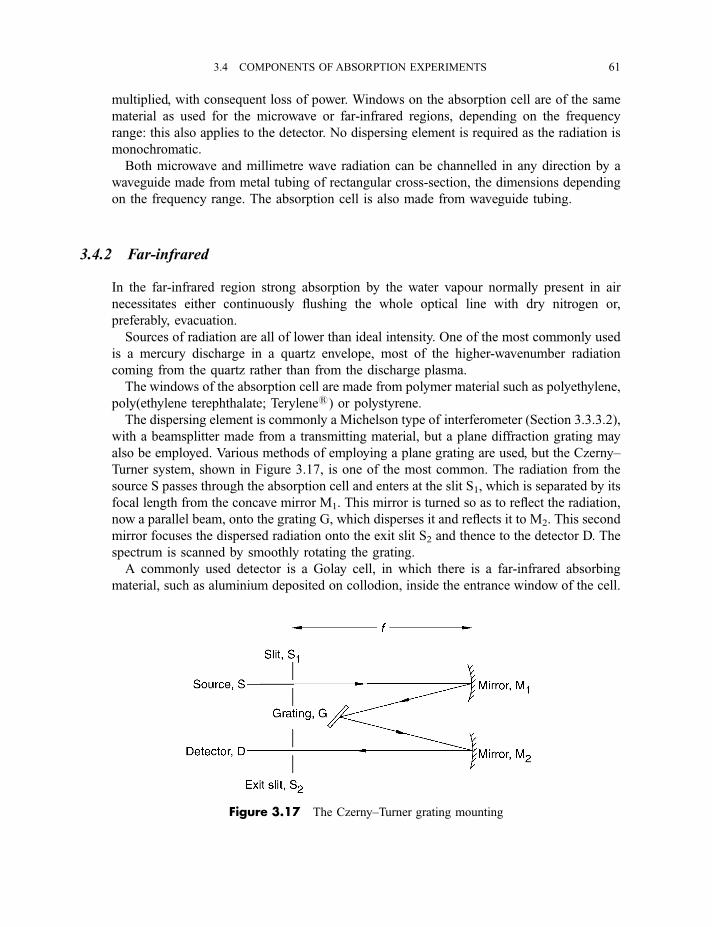
multiplied, with consequent loss of power. Windows on the absorption cell are of the same
material as used for the microwave or far-infrared regions, depending on the frequency
range: this also applies to the detector. No dispersing element is required as the radiation is
monochromatic.
Both microwave and millimetre wave radiation can be channelled in any direction by a
waveguide made from metal tubing of rectangular cross-section, the dimensions depending
on the frequency range. The absorption cell is also made from waveguide tubing.
3.4.2 Far-infrared
In the far-infrared region strong absorption by the water vapour normally present in air
necessitates either continuously flushing the whole optical line with dry nitrogen or,
preferably, evacuation.
Sources of radiation are all of lower than ideal intensity. One of the most commonly used
is a mercury discharge in a quartz envelope, most of the higher-wavenumber radiation
coming from the quartz rather than from the discharge plasma.
The windows of the absorption cell are made from polymer material such as polyethylene,
poly(ethylene terephthalate; Terylene1) or polystyrene.
The dispersing element is commonly a Michelson type of interferometer (Section 3.3.3.2),
with a beamsplitter made from a transmitting material, but a plane diffraction grating may
also be employed. Various methods of employing a plane grating are used, but the Czerny–
Turner system, shown in Figure 3.17, is one of the most common. The radiation from the
source S passes through the absorption cell and enters at the slit S1, which is separated by its
focal length from the concave mirror M1. This mirror is turned so as to reflect the radiation,
now a parallel beam, onto the grating G, which disperses it and reflects it to M2. This second
mirror focuses the dispersed radiation onto the exit slit S2 and thence to the detector D. The
spectrum is scanned by smoothly rotating the grating.
A commonly used detector is a Golay cell, in which there is a far-infrared absorbing
material, such as aluminium deposited on collodion, inside the entrance window of the cell.
Figure 3.17 The Czerny–Turner grating mounting
3.4 COMPONENTS OF ABSORPTION EXPERIMENTS 61
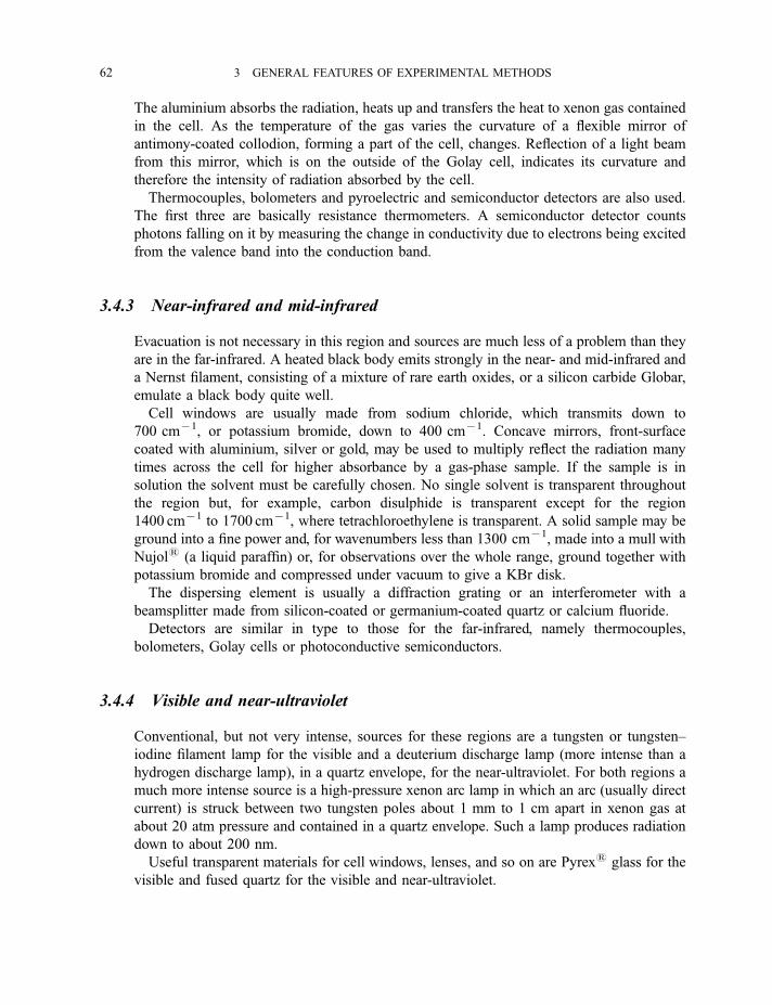
The aluminium absorbs the radiation, heats up and transfers the heat to xenon gas contained
in the cell. As the temperature of the gas varies the curvature of a flexible mirror of
antimony-coated collodion, forming a part of the cell, changes. Reflection of a light beam
from this mirror, which is on the outside of the Golay cell, indicates its curvature and
therefore the intensity of radiation absorbed by the cell.
Thermocouples, bolometers and pyroelectric and semiconductor detectors are also used.
The first three are basically resistance thermometers. A semiconductor detector counts
photons falling on it by measuring the change in conductivity due to electrons being excited
from the valence band into the conduction band.
3.4.3 Near-infrared and mid-infrared
Evacuation is not necessary in this region and sources are much less of a problem than they
are in the far-infrared. A heated black body emits strongly in the near- and mid-infrared and
a Nernst filament, consisting of a mixture of rare earth oxides, or a silicon carbide Globar,
emulate a black body quite well.
Cell windows are usually made from sodium chloride, which transmits down to
700 cm71, or potassium bromide, down to 400 cm71. Concave mirrors, front-surface
coated with aluminium, silver or gold, may be used to multiply reflect the radiation many
times across the cell for higher absorbance by a gas-phase sample. If the sample is in
solution the solvent must be carefully chosen. No single solvent is transparent throughout
the region but, for example, carbon disulphide is transparent except for the region
1400 cm71 to 1700 cm71, where tetrachloroethylene is transparent. A solid sample may be
ground into a fine power and, for wavenumbers less than 1300 cm71, made into a mull with
Nujol1 (a liquid paraffin) or, for observations over the whole range, ground together with
potassium bromide and compressed under vacuum to give a KBr disk.
The dispersing element is usually a diffraction grating or an interferometer with a
beamsplitter made from silicon-coated or germanium-coated quartz or calcium fluoride.
Detectors are similar in type to those for the far-infrared, namely thermocouples,
bolometers, Golay cells or photoconductive semiconductors.
3.4.4 Visible and near-ultraviolet
Conventional, but not very intense, sources for these regions are a tungsten or tungsten–
iodine filament lamp for the visible and a deuterium discharge lamp (more intense than a
hydrogen discharge lamp), in a quartz envelope, for the near-ultraviolet. For both regions a
much more intense source is a high-pressure xenon arc lamp in which an arc (usually direct
current) is struck between two tungsten poles about 1 mm to 1 cm apart in xenon gas at
about 20 atm pressure and contained in a quartz envelope. Such a lamp produces radiation
down to about 200 nm.
Useful transparent materials for cell windows, lenses, and so on are Pyrex1 glass for the
visible and fused quartz for the visible and near-ultraviolet.
62 3 GENERAL FEATURES OF EXPERIMENTAL METHODS
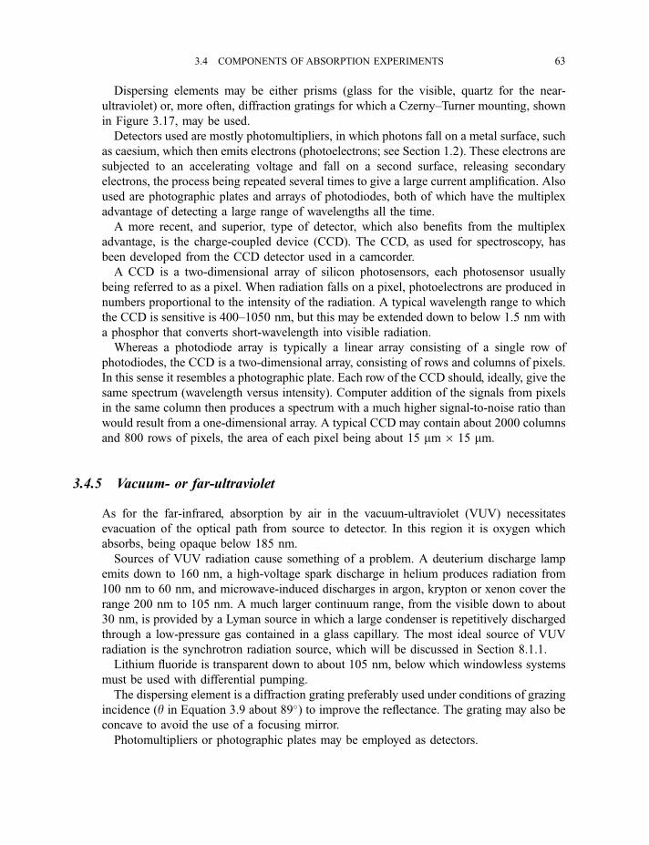
Dispersing elements may be either prisms (glass for the visible, quartz for the near-
ultraviolet) or, more often, diffraction gratings for which a Czerny–Turner mounting, shown
in Figure 3.17, may be used.
Detectors used are mostly photomultipliers, in which photons fall on a metal surface, such
as caesium, which then emits electrons (photoelectrons; see Section 1.2). These electrons are
subjected to an accelerating voltage and fall on a second surface, releasing secondary
electrons, the process being repeated several times to give a large current amplification. Also
used are photographic plates and arrays of photodiodes, both of which have the multiplex
advantage of detecting a large range of wavelengths all the time.
A more recent, and superior, type of detector, which also benefits from the multiplex
advantage, is the charge-coupled device (CCD). The CCD, as used for spectroscopy, has
been developed from the CCD detector used in a camcorder.
A CCD is a two-dimensional array of silicon photosensors, each photosensor usually
being referred to as a pixel. When radiation falls on a pixel, photoelectrons are produced in
numbers proportional to the intensity of the radiation. A typical wavelength range to which
the CCD is sensitive is 400–1050 nm, but this may be extended down to below 1.5 nm with
a phosphor that converts short-wavelength into visible radiation.
Whereas a photodiode array is typically a linear array consisting of a single row of
photodiodes, the CCD is a two-dimensional array, consisting of rows and columns of pixels.
In this sense it resembles a photographic plate. Each row of the CCD should, ideally, give the
same spectrum (wavelength versus intensity). Computer addition of the signals from pixels
in the same column then produces a spectrum with a much higher signal-to-noise ratio than
would result from a one-dimensional array. A typical CCD may contain about 2000 columns
and 800 rows of pixels, the area of each pixel being about 15 mm6 15 mm.
3.4.5 Vacuum- or far-ultraviolet
As for the far-infrared, absorption by air in the vacuum-ultraviolet (VUV) necessitates
evacuation of the optical path from source to detector. In this region it is oxygen which
absorbs, being opaque below 185 nm.
Sources of VUV radiation cause something of a problem. A deuterium discharge lamp
emits down to 160 nm, a high-voltage spark discharge in helium produces radiation from
100 nm to 60 nm, and microwave-induced discharges in argon, krypton or xenon cover the
range 200 nm to 105 nm. A much larger continuum range, from the visible down to about
30 nm, is provided by a Lyman source in which a large condenser is repetitively discharged
through a low-pressure gas contained in a glass capillary. The most ideal source of VUV
radiation is the synchrotron radiation source, which will be discussed in Section 8.1.1.
Lithium fluoride is transparent down to about 105 nm, below which windowless systems
must be used with differential pumping.
The dispersing element is a diffraction grating preferably used under conditions of grazing
incidence (y in Equation 3.9 about 89�) to improve the reflectance. The grating may also be
concave to avoid the use of a focusing mirror.
Photomultipliers or photographic plates may be employed as detectors.
3.4 COMPONENTS OF ABSORPTION EXPERIMENTS 63
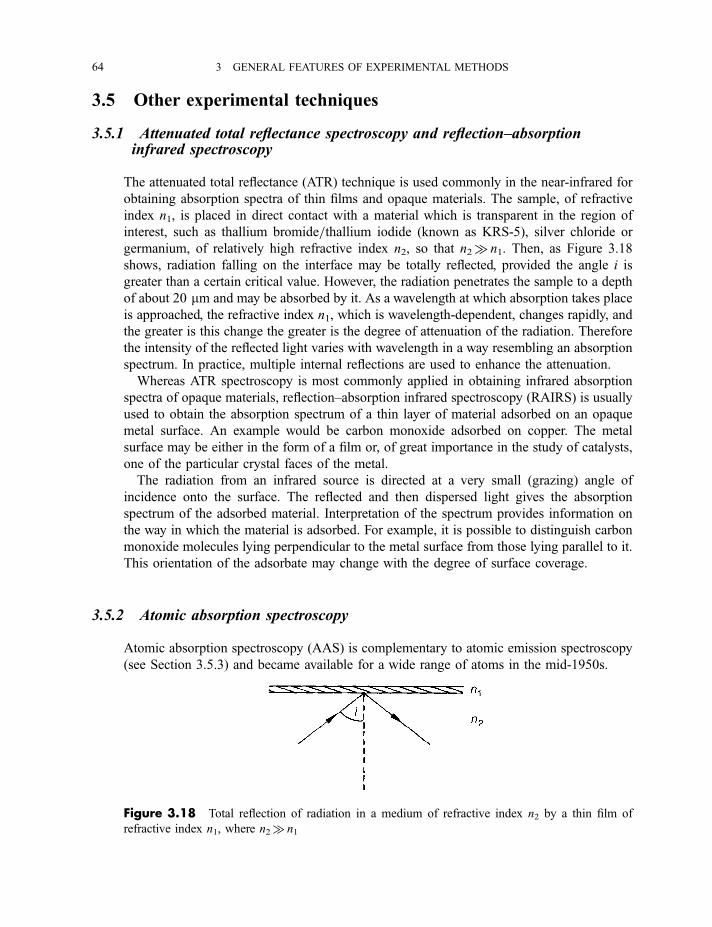
3.5 Other experimental techniques
3.5.1 Attenuated total reflectance spectroscopy and reflection–absorptioninfrared spectroscopy
The attenuated total reflectance (ATR) technique is used commonly in the near-infrared for
obtaining absorption spectra of thin films and opaque materials. The sample, of refractive
index n1, is placed in direct contact with a material which is transparent in the region of
interest, such as thallium bromide=thallium iodide (known as KRS-5), silver chloride or
germanium, of relatively high refractive index n2, so that n2 n1. Then, as Figure 3.18
shows, radiation falling on the interface may be totally reflected, provided the angle i is
greater than a certain critical value. However, the radiation penetrates the sample to a depth
of about 20 mm and may be absorbed by it. As a wavelength at which absorption takes place
is approached, the refractive index n1, which is wavelength-dependent, changes rapidly, and
the greater is this change the greater is the degree of attenuation of the radiation. Therefore
the intensity of the reflected light varies with wavelength in a way resembling an absorption
spectrum. In practice, multiple internal reflections are used to enhance the attenuation.
Whereas ATR spectroscopy is most commonly applied in obtaining infrared absorption
spectra of opaque materials, reflection–absorption infrared spectroscopy (RAIRS) is usually
used to obtain the absorption spectrum of a thin layer of material adsorbed on an opaque
metal surface. An example would be carbon monoxide adsorbed on copper. The metal
surface may be either in the form of a film or, of great importance in the study of catalysts,
one of the particular crystal faces of the metal.
The radiation from an infrared source is directed at a very small (grazing) angle of
incidence onto the surface. The reflected and then dispersed light gives the absorption
spectrum of the adsorbed material. Interpretation of the spectrum provides information on
the way in which the material is adsorbed. For example, it is possible to distinguish carbon
monoxide molecules lying perpendicular to the metal surface from those lying parallel to it.
This orientation of the adsorbate may change with the degree of surface coverage.
3.5.2 Atomic absorption spectroscopy
Atomic absorption spectroscopy (AAS) is complementary to atomic emission spectroscopy
(see Section 3.5.3) and became available for a wide range of atoms in the mid-1950s.
Figure 3.18 Total reflection of radiation in a medium of refractive index n2 by a thin film of
refractive index n1, where n2 n1
64 3 GENERAL FEATURES OF EXPERIMENTAL METHODS
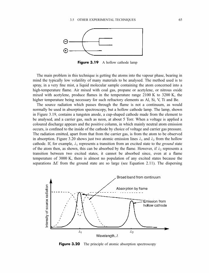
The main problem in this technique is getting the atoms into the vapour phase, bearing in
mind the typically low volatility of many materials to be analysed. The method used is to
spray, in a very fine mist, a liquid molecular sample containing the atom concerned into a
high-temperature flame. Air mixed with coal gas, propane or acetylene, or nitrous oxide
mixed with acetylene, produce flames in the temperature range 2100 K to 3200 K, the
higher temperature being necessary for such refractory elements as Al, Si, V, Ti and Be.
The source radiation which passes through the flame is not a continuum, as would
normally be used in absorption spectroscopy, but a hollow cathode lamp. The lamp, shown
in Figure 3.19, contains a tungsten anode, a cup-shaped cathode made from the element to
be analysed, and a carrier gas, such as neon, at about 5 Torr. When a voltage is applied a
coloured discharge appears and the positive column, in which mainly neutral atom emission
occurs, is confined to the inside of the cathode by choice of voltage and carrier gas pressure.
The radiation emitted, apart from that from the carrier gas, is from the atom to be observed
in absorption. Figure 3.20 shows just two atomic emission lines l1 and l2 from the hollow
cathode. If, for example, l1 represents a transition from an excited state to the ground state
of the atom then, as shown, this can be absorbed by the flame. However, if l2 represents atransition between two excited states, it cannot be absorbed since, even at a flame
temperature of 3000 K, there is almost no population of any excited states because the
separations DE from the ground state are so large (see Equation 2.11). The dispersing
Figure 3.19 A hollow cathode lamp
Figure 3.20 The principle of atomic absorption spectroscopy
3.5 OTHER EXPERIMENTAL TECHNIQUES 65
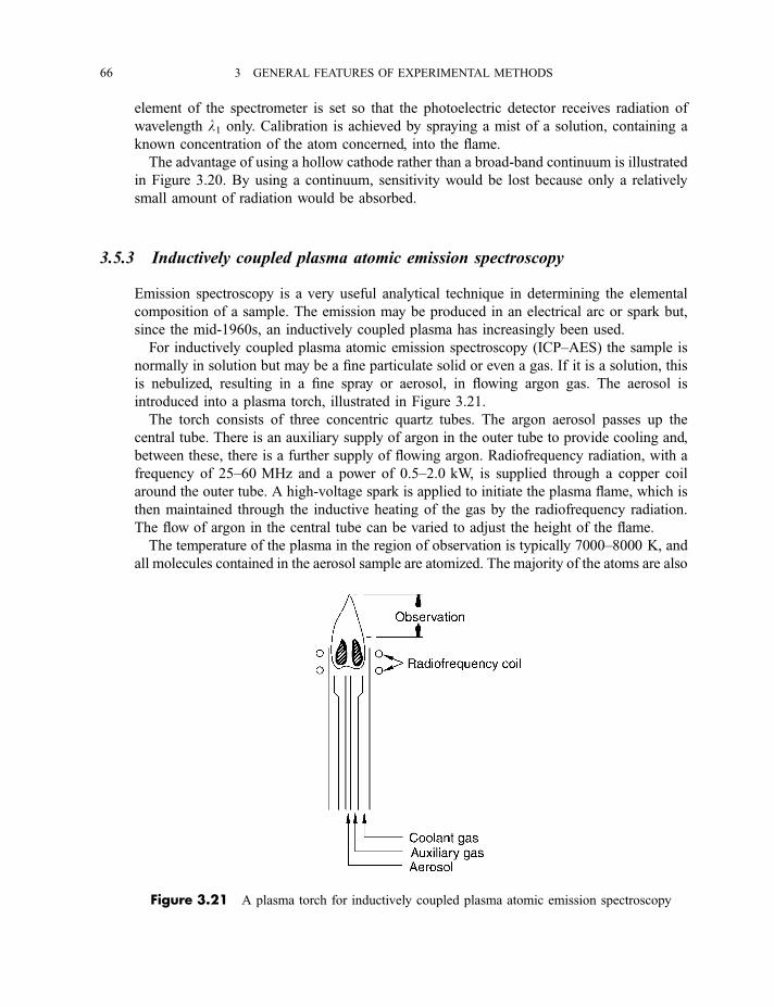
element of the spectrometer is set so that the photoelectric detector receives radiation of
wavelength l1 only. Calibration is achieved by spraying a mist of a solution, containing a
known concentration of the atom concerned, into the flame.
The advantage of using a hollow cathode rather than a broad-band continuum is illustrated
in Figure 3.20. By using a continuum, sensitivity would be lost because only a relatively
small amount of radiation would be absorbed.
3.5.3 Inductively coupled plasma atomic emission spectroscopy
Emission spectroscopy is a very useful analytical technique in determining the elemental
composition of a sample. The emission may be produced in an electrical arc or spark but,
since the mid-1960s, an inductively coupled plasma has increasingly been used.
For inductively coupled plasma atomic emission spectroscopy (ICP–AES) the sample is
normally in solution but may be a fine particulate solid or even a gas. If it is a solution, this
is nebulized, resulting in a fine spray or aerosol, in flowing argon gas. The aerosol is
introduced into a plasma torch, illustrated in Figure 3.21.
The torch consists of three concentric quartz tubes. The argon aerosol passes up the
central tube. There is an auxiliary supply of argon in the outer tube to provide cooling and,
between these, there is a further supply of flowing argon. Radiofrequency radiation, with a
frequency of 25–60 MHz and a power of 0.5–2.0 kW, is supplied through a copper coil
around the outer tube. A high-voltage spark is applied to initiate the plasma flame, which is
then maintained through the inductive heating of the gas by the radiofrequency radiation.
The flow of argon in the central tube can be varied to adjust the height of the flame.
The temperature of the plasma in the region of observation is typically 7000–8000 K, and
all molecules contained in the aerosol sample are atomized. The majority of the atoms are also
Figure 3.21 A plasma torch for inductively coupled plasma atomic emission spectroscopy
66 3 GENERAL FEATURES OF EXPERIMENTAL METHODS
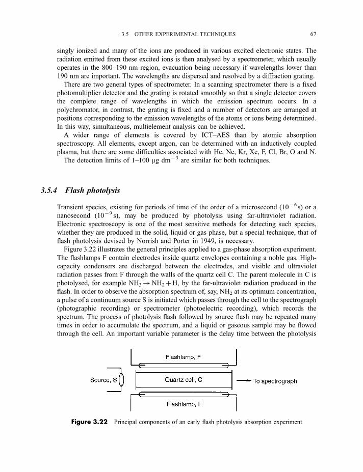
singly ionized and many of the ions are produced in various excited electronic states. The
radiation emitted from these excited ions is then analysed by a spectrometer, which usually
operates in the 800–190 nm region, evacuation being necessary if wavelengths lower than
190 nm are important. The wavelengths are dispersed and resolved by a diffraction grating.
There are two general types of spectrometer. In a scanning spectrometer there is a fixed
photomultiplier detector and the grating is rotated smoothly so that a single detector covers
the complete range of wavelengths in which the emission spectrum occurs. In a
polychromator, in contrast, the grating is fixed and a number of detectors are arranged at
positions corresponding to the emission wavelengths of the atoms or ions being determined.
In this way, simultaneous, multielement analysis can be achieved.
A wider range of elements is covered by ICT–AES than by atomic absorption
spectroscopy. All elements, except argon, can be determined with an inductively coupled
plasma, but there are some difficulties associated with He, Ne, Kr, Xe, F, Cl, Br, O and N.
The detection limits of 1–100 mg dm73 are similar for both techniques.
3.5.4 Flash photolysis
Transient species, existing for periods of time of the order of a microsecond (1076 s) or a
nanosecond (1079 s), may be produced by photolysis using far-ultraviolet radiation.
Electronic spectroscopy is one of the most sensitive methods for detecting such species,
whether they are produced in the solid, liquid or gas phase, but a special technique, that of
flash photolysis devised by Norrish and Porter in 1949, is necessary.
Figure 3.22 illustrates the general principles applied to a gas-phase absorption experiment.
The flashlamps F contain electrodes inside quartz envelopes containing a noble gas. High-
capacity condensers are discharged between the electrodes, and visible and ultraviolet
radiation passes from F through the walls of the quartz cell C. The parent molecule in C is
photolysed, for example NH3!NH2þH, by the far-ultraviolet radiation produced in the
flash. In order to observe the absorption spectrum of, say, NH2 at its optimum concentration,
a pulse of a continuum source S is initiated which passes through the cell to the spectrograph
(photographic recording) or spectrometer (photoelectric recording), which records the
spectrum. The process of photolysis flash followed by source flash may be repeated many
times in order to accumulate the spectrum, and a liquid or gaseous sample may be flowed
through the cell. An important variable parameter is the delay time between the photolysis
Figure 3.22 Principal components of an early flash photolysis absorption experiment
3.5 OTHER EXPERIMENTAL TECHNIQUES 67
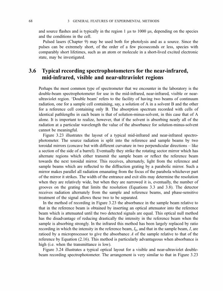
and source flashes and is typically in the region 1 ms to 1000 ms, depending on the species
and the conditions in the cell.
Pulsed lasers (Chapter 9) may be used both for photolysis and as a source. Since the
pulses can be extremely short, of the order of a few picoseconds or less, species with
comparably short lifetimes, such as an atom or molecule in a short-lived excited electronic
state, may be investigated.
3.6 Typical recording spectrophotometers for the near-infrared,mid-infrared, visible and near-ultraviolet regions
Perhaps the most common type of spectrometer that we encounter in the laboratory is the
double-beam spectrophotometer for use in the mid-infrared, near-infrared, visible or near-
ultraviolet region. ‘Double beam’ refers to the facility of having two beams of continuum
radiation, one for a sample cell containing, say, a solution of A in a solvent B and the other
for a reference cell containing only B. The absorption spectrum recorded with cells of
identical pathlengths in each beam is that of solution-minus-solvent, in this case that of A
alone. It is important to realize, however, that if the solvent is absorbing nearly all of the
radiation at a particular wavelength the value of the absorbance for solution-minus-solvent
cannot be meaningful.
Figure 3.23 illustrates the layout of a typical mid-infrared and near-infrared spectro-
photometer. The source radiation is split into the reference and sample beams by two
toroidal mirrors (concave but with different curvature in two perpendicular directions – like
a section of the side of a barrel). Eventually they strike the rotating sector mirror which has
alternate regions which either transmit the sample beam or reflect the reference beam
towards the next toroidal mirror. This receives, alternately, light from the reference and
sample beams which are reflected to the diffraction grating by a parabolic mirror. Such a
mirror makes parallel all radiation emanating from the focus of the parabola whichever part
of the mirror it strikes. The width of the entrance and exit slits may determine the resolution
when they are relatively wide, but when they are narrowed it is, eventually, the number of
grooves on the grating that limits the resolution (Equations 3.3 and 3.8). The detector
receives radiation alternately from the sample and reference beams, and phase-sensitive
treatment of the signal allows these two to be separated.
In the method of recording in Figure 3.23 the absorbance in the sample beam relative to
that in the reference beam is obtained by inserting an optical attenuator into the reference
beam which is attenuated until the two detected signals are equal. This optical null method
has the disadvantage of reducing drastically the intensity in the reference beam when the
sample is absorbing strongly. In the infrared this method has been largely replaced by ratio
recording in which the intensity in the reference beam, I0, and that in the sample beam, I, are
ratioed by a microprocessor to give the absorbance A of the sample relative to that of the
reference by Equation (2.16). This method is particularly advantageous when absorbance is
high (i.e. when the transmittance is low).
Figure 3.24 illustrates a typical optical layout for a visible and near-ultraviolet double-
beam recording spectrophotometer. The arrangement is very similar to that in Figure 3.23
68 3 GENERAL FEATURES OF EXPERIMENTAL METHODS
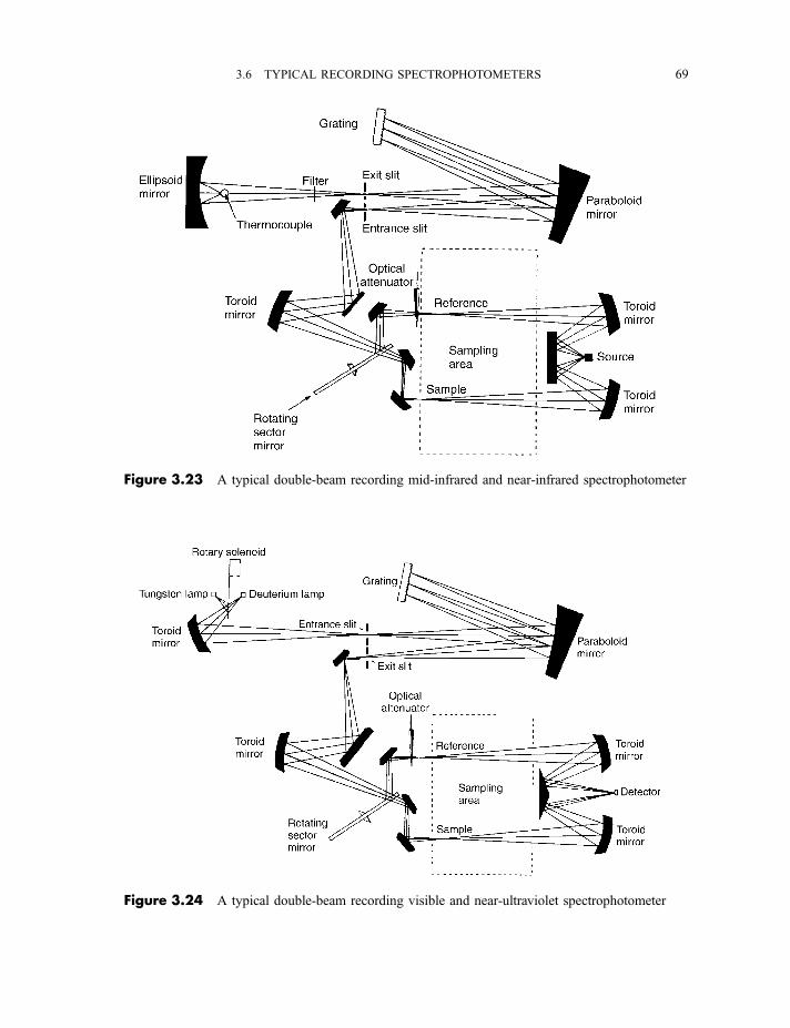
Figure 3.23 A typical double-beam recording mid-infrared and near-infrared spectrophotometer
Figure 3.24 A typical double-beam recording visible and near-ultraviolet spectrophotometer
3.6 TYPICAL RECORDING SPECTROPHOTOMETERS 69
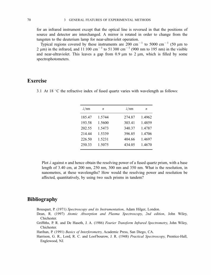
for an infrared instrument except that the optical line is reversed in that the positions of
source and detector are interchanged. A mirror is rotated in order to change from the
tungsten to the deuterium lamp for near-ultraviolet operation.
Typical regions covered by these instruments are 200 cm71 to 5000 cm71 (50 mm to
2 mm) in the infrared, and 11 100 cm71 to 51 300 cm71 (900 nm to 195 nm) in the visible
and near-ultraviolet. This leaves a gap from 0.9 mm to 2 mm, which is filled by some
spectrophotometers.
Exercise
3.1 At 18 �C the refractive index of fused quartz varies with wavelength as follows:
l=nm n l=nm n
185.47 1.5744 274.87 1.4962
193.58 1.5600 303.41 1.4859
202.55 1.5473 340.37 1.4787
214.44 1.5339 396.85 1.4706
226.50 1.5231 404.66 1.4697
250.33 1.5075 434.05 1.4670
Plot l against n and hence obtain the resolving power of a fused quartz prism, with a base
length of 3.40 cm, at 200 nm, 250 nm, 300 nm and 350 nm. What is the resolution, in
nanometres, at these wavelengths? How would the resolving power and resolution be
affected, quantitatively, by using two such prisms in tandem?
Bibliography
Bousquet, P. (1971) Spectroscopy and its Instrumentation, Adam Hilger, London.
Dean, R. (1997) Atomic Absorption and Plasma Spectroscopy, 2nd edition, John Wiley,
Chichester.
Griffiths, P. R. and De Haseth, J. A. (1986) Fourier Transform Infrared Spectrometry, John Wiley,
Chichester.
Harihan, P. (1991) Basics of Interferometry, Academic Press, San Diego, CA.
Harrison, G. R., Lord, R. C. and Loof bourow, J. R. (1948) Practical Spectroscopy, Prentice-Hall,
Englewood, NJ.
70 3 GENERAL FEATURES OF EXPERIMENTAL METHODS

Hecht, H. and Zajac, A. (1974) Optics, Addison-Wesley, Reading, MA.
Jenkins, F. A. and White, H. E. (1957) Fundamentals of Optics, McGraw-Hill, New York.
Longhurst, R. S. (1957) Geometrical and Physical Optics, Longman, London.
Sawyer, R. A. (1963) Experimental Spectroscopy, Dover, New York.
Sneddon, J., Thiem, T. and Lee, Y.-I. (1997) Lasers in Atomic Spectroscopy, John Wiley, New York.
BIBLIOGRAPHY 71

4Molecular Symmetry
The theory of molecular symmetry provides a satisfying and unifying thread which extends
throughout spectroscopy and valence theory. Although it is possible to understand atoms and
diatomic molecules without this theory, when it comes to understanding, say, spectroscopic
selection rules in polyatomic molecules, molecular symmetry presents a small barrier which
must be surmounted. However, for those not needing to progress so far this chapter may be
bypassed without too much hindrance.
The application of symmetry arguments to atoms and molecules has its origins in group
theory developed by mathematicians in the early nineteenth century, but it was not until the
1920s and 1930s that it was applied to atoms and molecules. It is because of this historical
development that the teaching of the subject has often been preceded by a detailed treatment
of matrix algebra. However, it is possible to progress quite a long way in understanding
molecular symmetry without any such mathematical knowledge and it is such a treatment
that is adopted here.
4.1 Elements of symmetry
If we compare the symmetry of a circle, a square and a rectangle it is intuitively obvious that
the degree of symmetry decreases in the order given. What about the degrees of symmetry of
a parallelogram and an isosceles triangle? Similarly, there is a decrease in the degree of
symmetry along the series of molecules ethylene, 1,1-difluoroethylene and fluoroethylene,
shown in Figure 4.1. However, cis- and trans-1,2-difluoroethylene also shown in the figure,
present a similar problem to the parallelogram and isosceles triangle. In fact, it will be
apparent by the end of this section that cis-1,2-difluoroethylene and an isosceles triangle
have the same symmetry as also do trans-1,2-difluoroethylene and a parallelogram.
These simple examples serve to show that instinctive ideas about symmetry are not going
to get us very far. We must put symmetry classification on a much firmer footing if it is to be
useful. In order to do this we need to define only five types of elements of symmetry – and
one of these is almost trivial. In discussing these we refer only to the free molecule, realized
in the gas phase at low pressure, and not, for example, to crystals which have additional
elements of symmetry relating the positions of different molecules within the unit cell. We
shall use, therefore, the Schonflies notation rather than the Hermann–Mauguin notation
favoured in crystallography.
In discussing molecular symmetry it is essential that the molecular shape is accurately
known, commonly by spectroscopic methods or by X-ray, electron or neutron diffraction.
73
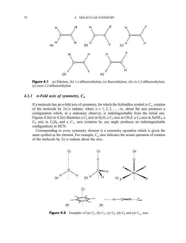
4.1.1 n-Fold axis of symmetry, Cn
If a molecule has an n-fold axis of symmetry, for which the Schonflies symbol is Cn, rotation
of the molecule by 2p=n radians, where n ¼ 1; 2; 3; . . . ;1, about the axis produces a
configuration which, to a stationary observer, is indistinguishable from the initial one.
Figures 4.2(a) to 4.2(e) illustrates a C2 axis in H2O, a C3 axis in CH3F, a C4 axis in XeOF4, a
C6 axis in C6H6 and a C? axis (rotation by any angle produces an indistinguishable
configuration) in HCN.
Corresponding to every symmetry element is a symmetry operation which is given the
same symbol as the element. For example, Cn also indicates the actual operation of rotation
of the molecule by 2p=n radians about the axis.
Figure 4.1 (a) Ethylene, (b) 1,1-difluoroethylene, (c) fluoroethylene, (d) cis-1,2-difluoroethylene,
(e) trans-1,2-difluoroethylene
Figure 4.2 Examples of (a) C2, (b) C3, (c) C4, (d) C6 and (e) C1 axes
74 4 MOLECULAR SYMMETRY
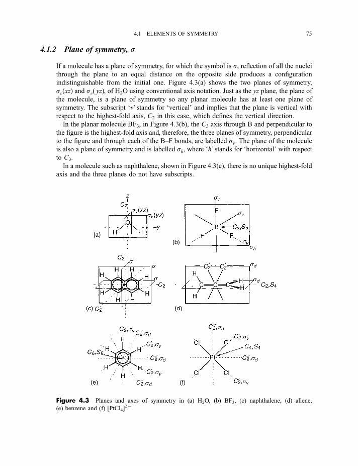
4.1.2 Plane of symmetry, s
If a molecule has a plane of symmetry, for which the symbol is s, reflection of all the nuclei
through the plane to an equal distance on the opposite side produces a configuration
indistinguishable from the initial one. Figure 4.3(a) shows the two planes of symmetry,
svðxzÞ and svð yzÞ, of H2O using conventional axis notation. Just as the yz plane, the plane of
the molecule, is a plane of symmetry so any planar molecule has at least one plane of
symmetry. The subscript ‘v’ stands for ‘vertical’ and implies that the plane is vertical with
respect to the highest-fold axis, C2 in this case, which defines the vertical direction.
In the planar molecule BF3, in Figure 4.3(b), the C3 axis through B and perpendicular to
the figure is the highest-fold axis and, therefore, the three planes of symmetry, perpendicular
to the figure and through each of the B–F bonds, are labelled sv. The plane of the molecule
is also a plane of symmetry and is labelled sh, where ‘h’ stands for ‘horizontal’ with respect
to C3.
In a molecule such as naphthalene, shown in Figure 4.3(c), there is no unique highest-fold
axis and the three planes do not have subscripts.
Figure 4.3 Planes and axes of symmetry in (a) H2O, (b) BF3, (c) naphthalene, (d) allene,
(e) benzene and (f) [PtCl4]27
4.1 ELEMENTS OF SYMMETRY 75
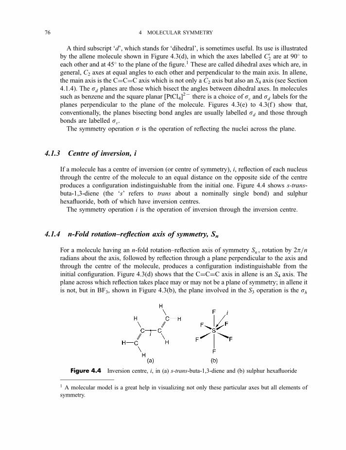
A third subscript ‘d’, which stands for ‘dihedral’, is sometimes useful. Its use is illustrated
by the allene molecule shown in Figure 4.3(d), in which the axes labelled C02 are at 90� toeach other and at 45� to the plane of the figure.1 These are called dihedral axes which are, in
general, C2 axes at equal angles to each other and perpendicular to the main axis. In allene,
the main axis is the C¼C¼C axis which is not only a C2 axis but also an S4 axis (see Section
4.1.4). The sd planes are those which bisect the angles between dihedral axes. In molecules
such as benzene and the square planar [PtCl4]27 there is a choice of sv and sd labels for the
planes perpendicular to the plane of the molecule. Figures 4.3(e) to 4.3(f ) show that,
conventionally, the planes bisecting bond angles are usually labelled sd and those through
bonds are labelled sv.The symmetry operation s is the operation of reflecting the nuclei across the plane.
4.1.3 Centre of inversion, i
If a molecule has a centre of inversion (or centre of symmetry), i, reflection of each nucleus
through the centre of the molecule to an equal distance on the opposite side of the centre
produces a configuration indistinguishable from the initial one. Figure 4.4 shows s-trans-
buta-1,3-diene (the ‘s’ refers to trans about a nominally single bond) and sulphur
hexafluoride, both of which have inversion centres.
The symmetry operation i is the operation of inversion through the inversion centre.
4.1.4 n-Fold rotation–reflection axis of symmetry, Sn
For a molecule having an n-fold rotation–reflection axis of symmetry Sn , rotation by 2p=nradians about the axis, followed by reflection through a plane perpendicular to the axis and
through the centre of the molecule, produces a configuration indistinguishable from the
initial configuration. Figure 4.3(d) shows that the C¼C¼C axis in allene is an S4 axis. The
plane across which reflection takes place may or may not be a plane of symmetry; in allene it
is not, but in BF3, shown in Figure 4.3(b), the plane involved in the S3 operation is the sh
Figure 4.4 Inversion centre, i, in (a) s-trans-buta-1,3-diene and (b) sulphur hexafluoride
1 A molecular model is a great help in visualizing not only these particular axes but all elements of
symmetry.
76 4 MOLECULAR SYMMETRY
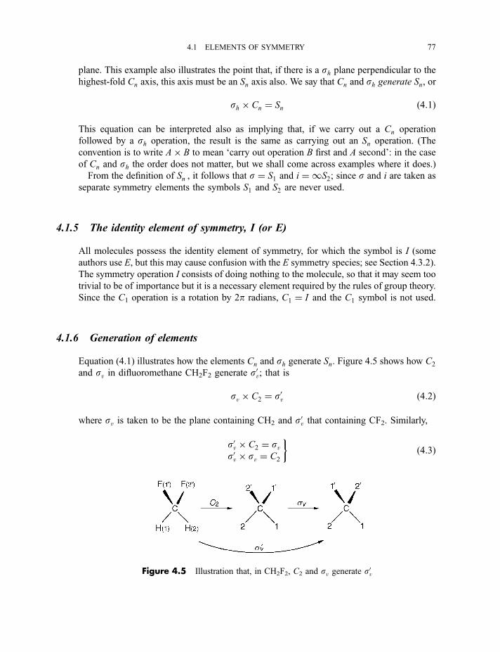
plane. This example also illustrates the point that, if there is a sh plane perpendicular to the
highest-fold Cn axis, this axis must be an Sn axis also. We say that Cn and sh generate Sn, or
sh � Cn ¼ Sn ð4:1Þ
This equation can be interpreted also as implying that, if we carry out a Cn operation
followed by a sh operation, the result is the same as carrying out an Sn operation. (The
convention is to write A� B to mean ‘carry out operation B first and A second’: in the case
of Cn and sh the order does not matter, but we shall come across examples where it does.)
From the definition of Sn , it follows that s ¼ S1 and i ¼ 1S2; since s and i are taken as
separate symmetry elements the symbols S1 and S2 are never used.
4.1.5 The identity element of symmetry, I (or E)
All molecules possess the identity element of symmetry, for which the symbol is I (some
authors use E, but this may cause confusion with the E symmetry species; see Section 4.3.2).
The symmetry operation I consists of doing nothing to the molecule, so that it may seem too
trivial to be of importance but it is a necessary element required by the rules of group theory.
Since the C1 operation is a rotation by 2p radians, C1 ¼ I and the C1 symbol is not used.
4.1.6 Generation of elements
Equation (4.1) illustrates how the elements Cn and sh generate Sn. Figure 4.5 shows how C2
and sv in difluoromethane CH2F2 generate s0v; that is
sv � C2 ¼ s0v ð4:2Þ
where sv is taken to be the plane containing CH2 and s0v that containing CF2. Similarly,
s0v � C2 ¼ svs0v � sv ¼ C2
�ð4:3Þ
Figure 4.5 Illustration that, in CH2F2, C2 and sv generate s0v
4.1 ELEMENTS OF SYMMETRY 77
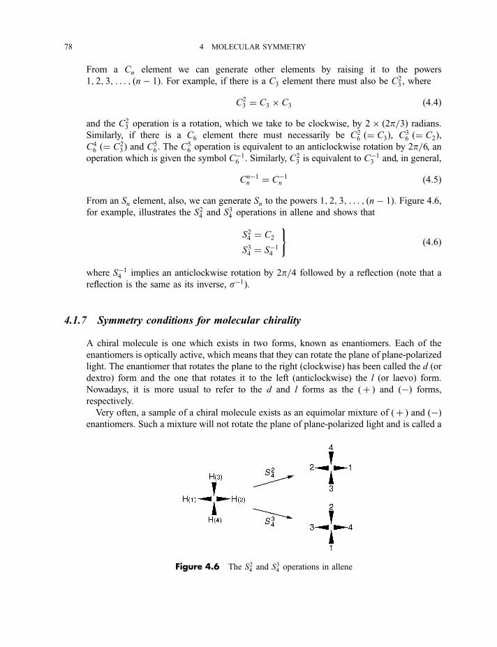
From a Cn element we can generate other elements by raising it to the powers
1; 2; 3; . . . ; ðn� 1Þ. For example, if there is a C3 element there must also be C23, where
C23 ¼ C3 � C3 ð4:4Þ
and the C23 operation is a rotation, which we take to be clockwise, by 2� ð2p=3Þ radians.
Similarly, if there is a C6 element there must necessarily be C26 ð¼ C3Þ, C3
6 ð¼ C2Þ,C46 ð¼ C2
3Þ and C56. The C
56 operation is equivalent to an anticlockwise rotation by 2p=6, an
operation which is given the symbol C�16 . Similarly, C23 is equivalent to C�13 and, in general,
Cn�1n ¼ C�1n ð4:5Þ
From an Sn element, also, we can generate Sn to the powers 1; 2; 3; . . . ; ðn� 1Þ. Figure 4.6,for example, illustrates the S24 and S34 operations in allene and shows that
S24 ¼ C2
S34 ¼ S�14
)ð4:6Þ
where S�14 implies an anticlockwise rotation by 2p=4 followed by a reflection (note that a
reflection is the same as its inverse, s�1).
4.1.7 Symmetry conditions for molecular chirality
A chiral molecule is one which exists in two forms, known as enantiomers. Each of the
enantiomers is optically active, which means that they can rotate the plane of plane-polarized
light. The enantiomer that rotates the plane to the right (clockwise) has been called the d (or
dextro) form and the one that rotates it to the left (anticlockwise) the l (or laevo) form.
Nowadays, it is more usual to refer to the d and l forms as the (þ ) and (�) forms,
respectively.
Very often, a sample of a chiral molecule exists as an equimolar mixture of (þ ) and (�)enantiomers. Such a mixture will not rotate the plane of plane-polarized light and is called a
Figure 4.6 The S24 and S34 operations in allene
78 4 MOLECULAR SYMMETRY
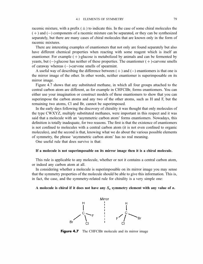
racemic mixture, with a prefix (� ) to indicate this. In the case of some chiral molecules the
(þ ) and (�) components of a racemic mixture can be separated, or they can be synthesized
separately, but there are many cases of chiral molecules that are known only in the form of
racemic mixtures.
There are interesting examples of enantiomers that not only are found separately but also
have different chemical properties when reacting with some reagent which is itself an
enantiomer. For example (þ )-glucose is metabolized by animals and can be fermented by
yeasts, but (�)-glucose has neither of these properties. The enantiomer (þ )-carvone smells
of caraway whereas (�)-carvone smells of spearmint.
A useful way of describing the difference between (þ ) and (�) enantiomers is that one is
the mirror image of the other. In other words, neither enantiomer is superimposable on its
mirror image.
Figure 4.7 shows that any substituted methane, in which all four groups attached to the
central carbon atom are different, as for example in CHFClBr, forms enantiomers. You can
either use your imagination or construct models of these enantiomers to show that you can
superimpose the carbon atoms and any two of the other atoms, such as H and F, but the
remaining two atoms, Cl and Br, cannot be superimposed.
In the early days following the discovery of chirality it was thought that only molecules of
the type CWXYZ, multiply substituted methanes, were important in this respect and it was
said that a molecule with an ‘asymmetric carbon atom’ forms enantiomers. Nowadays, this
definition is totally inadequate, for two reasons. The first is that the existence of enantiomers
is not confined to molecules with a central carbon atom (it is not even confined to organic
molecules), and the second is that, knowing what we do about the various possible elements
of symmetry, the phrase ‘asymmetric carbon atom’ has no real meaning.
One useful rule that does survive is that:
If a molecule is not superimposable on its mirror image then it is a chiral molecule.
This rule is applicable to any molecule, whether or not it contains a central carbon atom,
or indeed any carbon atom at all.
In considering whether a molecule is superimposable on its mirror image you may sense
that the symmetry properties of the molecule should be able to give this information. This is,
in fact, the case, and the symmetry-related rule for chirality is a very simple one:
A molecule is chiral if it does not have any Sn symmetry element with any value of n.
Figure 4.7 The CHFClBr molecule and its mirror image
4.1 ELEMENTS OF SYMMETRY 79
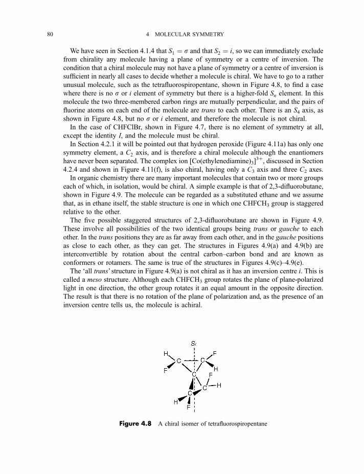
We have seen in Section 4.1.4 that S1 ¼ s and that S2 ¼ i, so we can immediately exclude
from chirality any molecule having a plane of symmetry or a centre of inversion. The
condition that a chiral molecule may not have a plane of symmetry or a centre of inversion is
sufficient in nearly all cases to decide whether a molecule is chiral. We have to go to a rather
unusual molecule, such as the tetrafluorospiropentane, shown in Figure 4.8, to find a case
where there is no s or i element of symmetry but there is a higher-fold Sn element. In this
molecule the two three-membered carbon rings are mutually perpendicular, and the pairs of
fluorine atoms on each end of the molecule are trans to each other. There is an S4 axis, as
shown in Figure 4.8, but no s or i element, and therefore the molecule is not chiral.
In the case of CHFClBr, shown in Figure 4.7, there is no element of symmetry at all,
except the identity I, and the molecule must be chiral.
In Section 4.2.1 it will be pointed out that hydrogen peroxide (Figure 4.11a) has only one
symmetry element, a C2 axis, and is therefore a chiral molecule although the enantiomers
have never been separated. The complex ion [Co(ethylenediamine)3]3þ, discussed in Section
4.2.4 and shown in Figure 4.11(f), is also chiral, having only a C3 axis and three C2 axes.
In organic chemistry there are many important molecules that contain two or more groups
each of which, in isolation, would be chiral. A simple example is that of 2,3-difluorobutane,
shown in Figure 4.9. The molecule can be regarded as a substituted ethane and we assume
that, as in ethane itself, the stable structure is one in which one CHFCH3 group is staggered
relative to the other.
The five possible staggered structures of 2,3-difluorobutane are shown in Figure 4.9.
These involve all possibilities of the two identical groups being trans or gauche to each
other. In the trans positions they are as far away from each other, and in the gauche positions
as close to each other, as they can get. The structures in Figures 4.9(a) and 4.9(b) are
interconvertible by rotation about the central carbon–carbon bond and are known as
conformers or rotamers. The same is true of the structures in Figures 4.9(c)–4.9(e).
The ‘all trans’ structure in Figure 4.9(a) is not chiral as it has an inversion centre i. This is
called a meso structure. Although each CHFCH3 group rotates the plane of plane-polarized
light in one direction, the other group rotates it an equal amount in the opposite direction.
The result is that there is no rotation of the plane of polarization and, as the presence of an
inversion centre tells us, the molecule is achiral.
Figure 4.8 A chiral isomer of tetrafluorospiropentane
80 4 MOLECULAR SYMMETRY
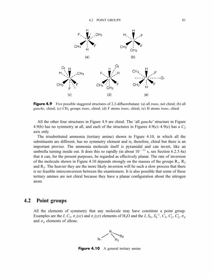
All the other four structures in Figure 4.9 are chiral. The ‘all gauche’ structure in Figure
4.9(b) has no symmetry at all, and each of the structures in Figures 4.9(c)–4.9(e) has a C2
axis only.
The trisubstituted ammonia (tertiary amine) shown in Figure 4.10, in which all the
substituents are different, has no symmetry element and is, therefore, chiral but there is an
important proviso. The ammonia molecule itself is pyramidal and can invert, like an
umbrella turning inside out. It does this so rapidly (in about 10711 s, see Section 6.2.5.4a)
that it can, for the present purposes, be regarded as effectively planar. The rate of inversion
of the molecule shown in Figure 4.10 depends strongly on the masses of the groups R1, R2
and R3. The heavier they are the more likely inversion will be such a slow process that there
is no feasible interconversion between the enantiomers. It is also possible that some of these
tertiary amines are not chiral because they have a planar configuration about the nitrogen
atom.
4.2 Point groups
All the elements of symmetry that any molecule may have constitute a point group.
Examples are the I, C2, svðxzÞ and svðyzÞ elements of H2O and the I, S4, S�14 , C2, C
02, C
02, sd
and sd elements of allene.
Figure 4.9 Five possible staggered structures of 2,3-difluorobutane: (a) all trans, not chiral; (b) all
gauche, chiral; (c) CH3 groups trans, chiral; (d) F atoms trans, chiral; (e) H atoms trans, chiral
Figure 4.10 A general tertiary amine
4.2 POINT GROUPS 81
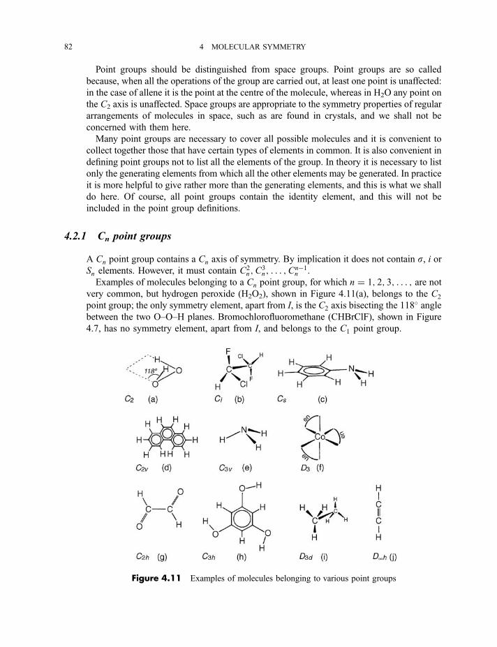
Point groups should be distinguished from space groups. Point groups are so called
because, when all the operations of the group are carried out, at least one point is unaffected:
in the case of allene it is the point at the centre of the molecule, whereas in H2O any point on
the C2 axis is unaffected. Space groups are appropriate to the symmetry properties of regular
arrangements of molecules in space, such as are found in crystals, and we shall not be
concerned with them here.
Many point groups are necessary to cover all possible molecules and it is convenient to
collect together those that have certain types of elements in common. It is also convenient in
defining point groups not to list all the elements of the group. In theory it is necessary to list
only the generating elements from which all the other elements may be generated. In practice
it is more helpful to give rather more than the generating elements, and this is what we shall
do here. Of course, all point groups contain the identity element, and this will not be
included in the point group definitions.
4.2.1 Cn point groups
A Cn point group contains a Cn axis of symmetry. By implication it does not contain s, i orSn elements. However, it must contain C2
n;C3n; . . . ;C
n�1n .
Examples of molecules belonging to a Cn point group, for which n ¼ 1; 2; 3; . . . ; are notvery common, but hydrogen peroxide (H2O2), shown in Figure 4.11(a), belongs to the C2
point group; the only symmetry element, apart from I, is the C2 axis bisecting the 118� angle
between the two O–O–H planes. Bromochlorofluoromethane (CHBrClF), shown in Figure
4.7, has no symmetry element, apart from I, and belongs to the C1 point group.
Figure 4.11 Examples of molecules belonging to various point groups
82 4 MOLECULAR SYMMETRY
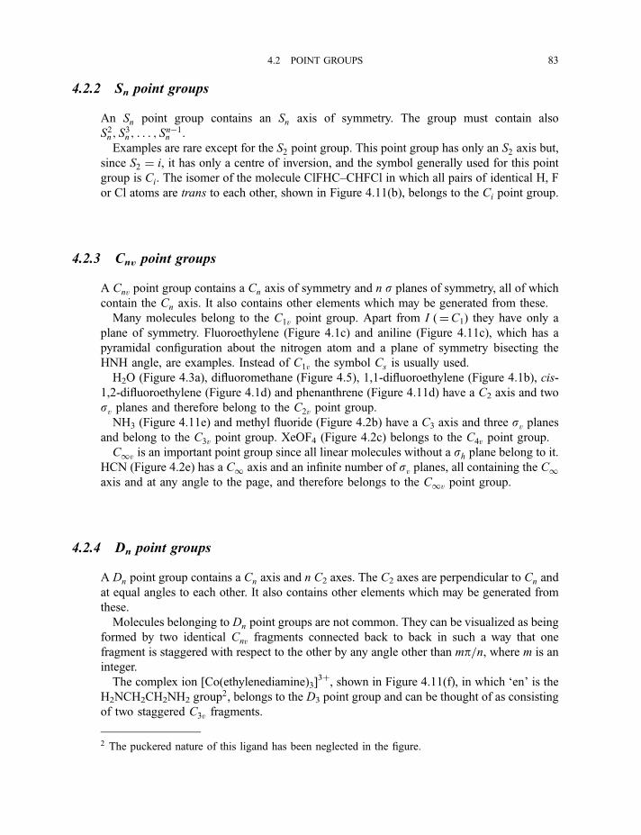
4.2.2 Sn point groups
An Sn point group contains an Sn axis of symmetry. The group must contain also
S2n ; S3n ; . . . ; S
n�1n .
Examples are rare except for the S2 point group. This point group has only an S2 axis but,
since S2 ¼ i, it has only a centre of inversion, and the symbol generally used for this point
group is Ci. The isomer of the molecule ClFHC–CHFCl in which all pairs of identical H, F
or Cl atoms are trans to each other, shown in Figure 4.11(b), belongs to the Ci point group.
4.2.3 Cnv point groups
A Cnv point group contains a Cn axis of symmetry and n s planes of symmetry, all of which
contain the Cn axis. It also contains other elements which may be generated from these.
Many molecules belong to the C1v point group. Apart from I (¼C1) they have only a
plane of symmetry. Fluoroethylene (Figure 4.1c) and aniline (Figure 4.11c), which has a
pyramidal configuration about the nitrogen atom and a plane of symmetry bisecting the
HNH angle, are examples. Instead of C1v the symbol Cs is usually used.
H2O (Figure 4.3a), difluoromethane (Figure 4.5), 1,1-difluoroethylene (Figure 4.1b), cis-
1,2-difluoroethylene (Figure 4.1d) and phenanthrene (Figure 4.11d) have a C2 axis and two
sv planes and therefore belong to the C2v point group.
NH3 (Figure 4.11e) and methyl fluoride (Figure 4.2b) have a C3 axis and three sv planesand belong to the C3v point group. XeOF4 (Figure 4.2c) belongs to the C4v point group.
C1v is an important point group since all linear molecules without a sh plane belong to it.
HCN (Figure 4.2e) has a C1 axis and an infinite number of sv planes, all containing the C1axis and at any angle to the page, and therefore belongs to the C1v point group.
4.2.4 Dn point groups
A Dn point group contains a Cn axis and n C2 axes. The C2 axes are perpendicular to Cn and
at equal angles to each other. It also contains other elements which may be generated from
these.
Molecules belonging to Dn point groups are not common. They can be visualized as being
formed by two identical Cnv fragments connected back to back in such a way that one
fragment is staggered with respect to the other by any angle other than mp=n, where m is an
integer.
The complex ion [Co(ethylenediamine)3]3þ, shown in Figure 4.11(f), in which ‘en’ is the
H2NCH2CH2NH2 group2, belongs to the D3 point group and can be thought of as consisting
of two staggered C3v fragments.
2 The puckered nature of this ligand has been neglected in the figure.
4.2 POINT GROUPS 83
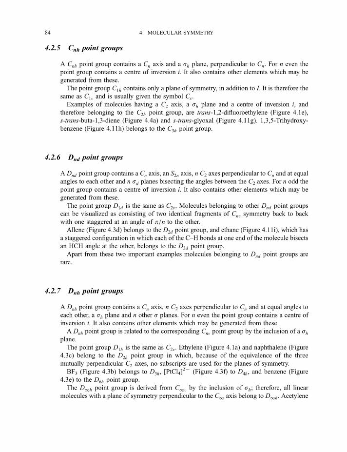
4.2.5 Cnh point groups
A Cnh point group contains a Cn axis and a sh plane, perpendicular to Cn. For n even the
point group contains a centre of inversion i. It also contains other elements which may be
generated from these.
The point group C1h contains only a plane of symmetry, in addition to I. It is therefore the
same as C1v and is usually given the symbol Cs.
Examples of molecules having a C2 axis, a sh plane and a centre of inversion i, and
therefore belonging to the C2h point group, are trans-1,2-difluoroethylene (Figure 4.1e),
s-trans-buta-1,3-diene (Figure 4.4a) and s-trans-glyoxal (Figure 4.11g). 1,3,5-Trihydroxy-
benzene (Figure 4.11h) belongs to the C3h point group.
4.2.6 Dnd point groups
A Dnd point group contains a Cn axis, an S2n axis, n C2 axes perpendicular to Cn and at equal
angles to each other and n sd planes bisecting the angles between the C2 axes. For n odd the
point group contains a centre of inversion i. It also contains other elements which may be
generated from these.
The point group D1d is the same as C2v. Molecules belonging to other Dnd point groups
can be visualized as consisting of two identical fragments of Cnv symmetry back to back
with one staggered at an angle of p=n to the other.
Allene (Figure 4.3d) belongs to the D2d point group, and ethane (Figure 4.11i), which has
a staggered configuration in which each of the C–H bonds at one end of the molecule bisects
an HCH angle at the other, belongs to the D3d point group.
Apart from these two important examples molecules belonging to Dnd point groups are
rare.
4.2.7 Dnh point groups
A Dnh point group contains a Cn axis, n C2 axes perpendicular to Cn and at equal angles to
each other, a sh plane and n other s planes. For n even the point group contains a centre of
inversion i. It also contains other elements which may be generated from these.
A Dnh point group is related to the corresponding Cnv point group by the inclusion of a shplane.
The point group D1h is the same as C2v. Ethylene (Figure 4.1a) and naphthalene (Figure
4.3c) belong to the D2h point group in which, because of the equivalence of the three
mutually perpendicular C2 axes, no subscripts are used for the planes of symmetry.
BF3 (Figure 4.3b) belongs to D3h, [PtCl4]27 (Figure 4.3f) to D4h, and benzene (Figure
4.3e) to the D6h point group.
The D1h point group is derived from C1v by the inclusion of sh; therefore, all linearmolecules with a plane of symmetry perpendicular to the C1 axis belong to D1h. Acetylene
84 4 MOLECULAR SYMMETRY
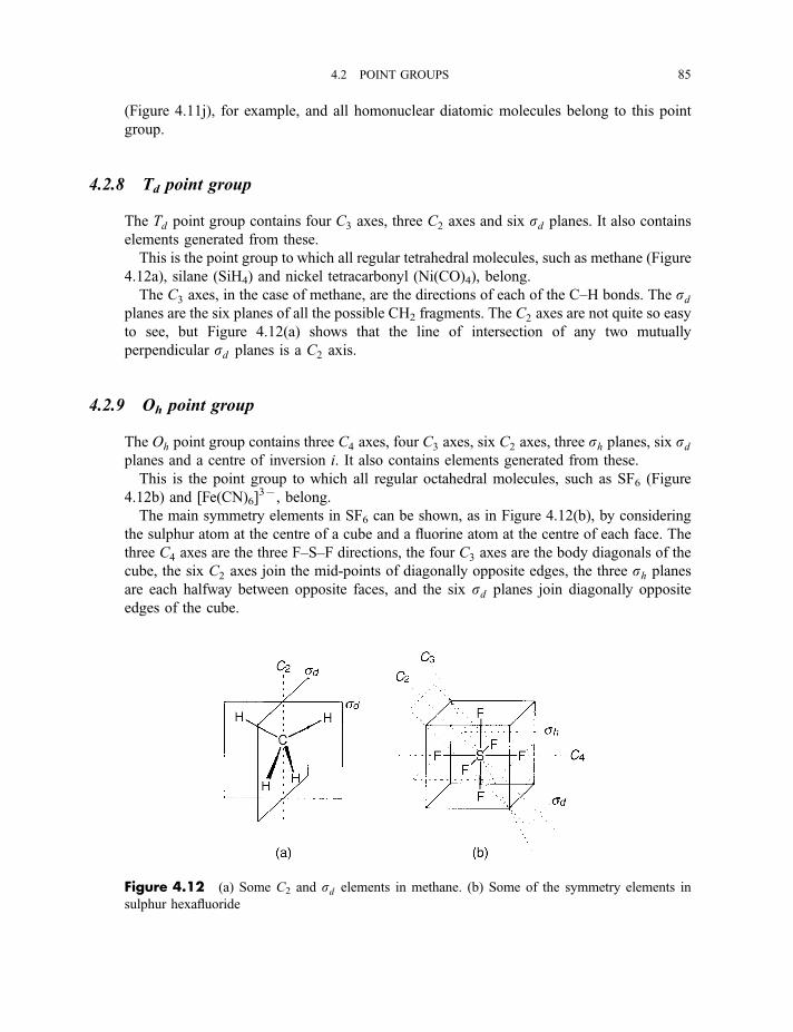
(Figure 4.11j), for example, and all homonuclear diatomic molecules belong to this point
group.
4.2.8 Td point group
The Td point group contains four C3 axes, three C2 axes and six sd planes. It also contains
elements generated from these.
This is the point group to which all regular tetrahedral molecules, such as methane (Figure
4.12a), silane (SiH4) and nickel tetracarbonyl (Ni(CO)4), belong.
The C3 axes, in the case of methane, are the directions of each of the C–H bonds. The sdplanes are the six planes of all the possible CH2 fragments. The C2 axes are not quite so easy
to see, but Figure 4.12(a) shows that the line of intersection of any two mutually
perpendicular sd planes is a C2 axis.
4.2.9 Oh point group
The Oh point group contains three C4 axes, four C3 axes, six C2 axes, three sh planes, six sdplanes and a centre of inversion i. It also contains elements generated from these.
This is the point group to which all regular octahedral molecules, such as SF6 (Figure
4.12b) and [Fe(CN)6]37, belong.
The main symmetry elements in SF6 can be shown, as in Figure 4.12(b), by considering
the sulphur atom at the centre of a cube and a fluorine atom at the centre of each face. The
three C4 axes are the three F–S–F directions, the four C3 axes are the body diagonals of the
cube, the six C2 axes join the mid-points of diagonally opposite edges, the three sh planes
are each halfway between opposite faces, and the six sd planes join diagonally opposite
edges of the cube.
Figure 4.12 (a) Some C2 and sd elements in methane. (b) Some of the symmetry elements in
sulphur hexafluoride
4.2 POINT GROUPS 85
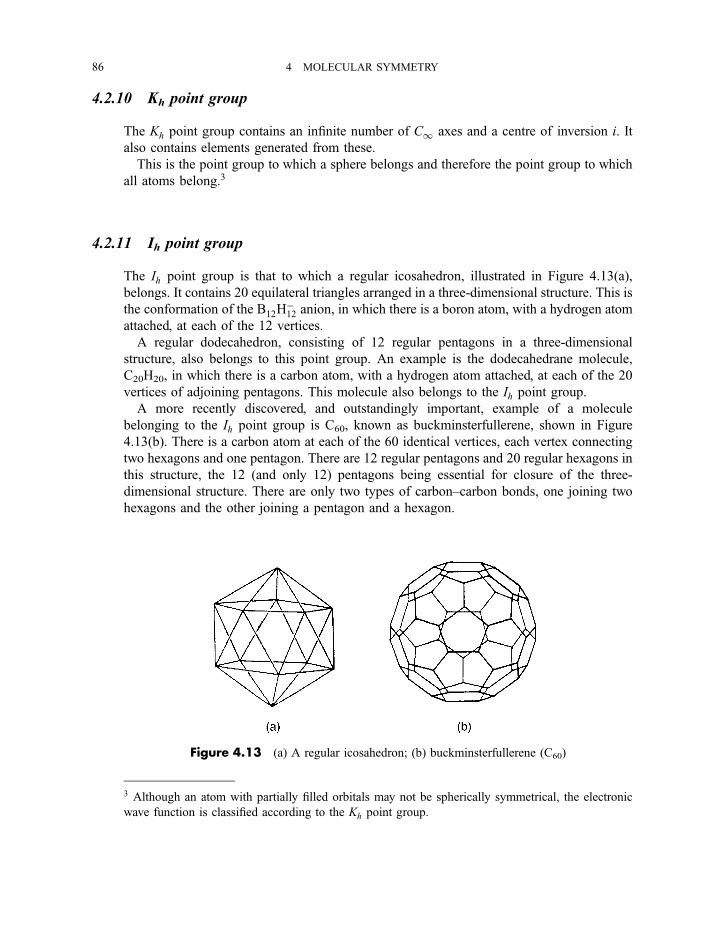
4.2.10 Kh point group
The Kh point group contains an infinite number of C1 axes and a centre of inversion i. It
also contains elements generated from these.
This is the point group to which a sphere belongs and therefore the point group to which
all atoms belong.3
4.2.11 Ih point group
The Ih point group is that to which a regular icosahedron, illustrated in Figure 4.13(a),
belongs. It contains 20 equilateral triangles arranged in a three-dimensional structure. This is
the conformation of the B12H�12 anion, in which there is a boron atom, with a hydrogen atom
attached, at each of the 12 vertices.
A regular dodecahedron, consisting of 12 regular pentagons in a three-dimensional
structure, also belongs to this point group. An example is the dodecahedrane molecule,
C20H20, in which there is a carbon atom, with a hydrogen atom attached, at each of the 20
vertices of adjoining pentagons. This molecule also belongs to the Ih point group.
A more recently discovered, and outstandingly important, example of a molecule
belonging to the Ih point group is C60, known as buckminsterfullerene, shown in Figure
4.13(b). There is a carbon atom at each of the 60 identical vertices, each vertex connecting
two hexagons and one pentagon. There are 12 regular pentagons and 20 regular hexagons in
this structure, the 12 (and only 12) pentagons being essential for closure of the three-
dimensional structure. There are only two types of carbon–carbon bonds, one joining two
hexagons and the other joining a pentagon and a hexagon.
Figure 4.13 (a) A regular icosahedron; (b) buckminsterfullerene (C60)
3 Although an atom with partially filled orbitals may not be spherically symmetrical, the electronic
wave function is classified according to the Kh point group.
86 4 MOLECULAR SYMMETRY
Molecules belonging to the Ih point group are very highly symmetrical, having 15 C2
axes, 10 C3 axes, 6 C5 axes, 15 s planes, 10 S6 axes, 6 S10 axes and a centre of inversion i. In
addition to these symmetry elements are other elements which can be generated from them.
4.2.12 Other point groups
The point groups discussed here are all those that one is likely to use, but there are a few
very uncommon ones that have not been included: descriptions of these are to be found in
the books on molecular symmetry mentioned in the bibliography at the end of this chapter.
4.3 Point group character tables
Point groups may be divided into two important sets: non-degenerate and degenerate. A
degenerate point group contains a Cn axis, with n> 2, or an S4 axis. A molecule belonging
to such a point group may have degenerate properties, for example different electronic or
vibrational wave functions with identical associated energies, but a molecule belonging to a
non-degenerate point group cannot have degenerate properties.
In Sections 4.1 and 4.2 we have seen how the symmetry properties of the equilibrium
nuclear configuration of any molecule may be classified and the molecule assigned to a point
group. However, molecules may have properties, such as electronic and vibrational wave
functions, which do not preserve all the elements of symmetry, and it is the symmetry
classification of such properties with which character tables are concerned. We shall
consider in detail three such tables: that of C2v, an example of a non-degenerate point group;
that of C3v, an example of a degenerate point group; and that of C1v, an example of an
infinite group, which has an infinite number of elements.
4.3.1 C2v character table
A property such as a vibrational wave function of, say, H2O may or may not preserve an
element of symmetry. If it preserves the element, carrying out the corresponding symmetry
operation, for example sv, has no effect on the wave function, which we write as
cv !sv ðþ1Þcv ð4:7Þ
and we say that cv is symmetric to sv. The only other possibility, in a non-degenerate point
group, is that the wave function may be changed in sign by carrying out the operation:
cv !sv ð�1Þcv ð4:8Þ
in which case we say that cv is antisymmetric to sv. The þ1 of Equation (4.7) and the �1 of
Equation (4.8) are known as the character of, in this case, cv with respect to sv.
4.3 POINT GROUP CHARACTER TABLES 87
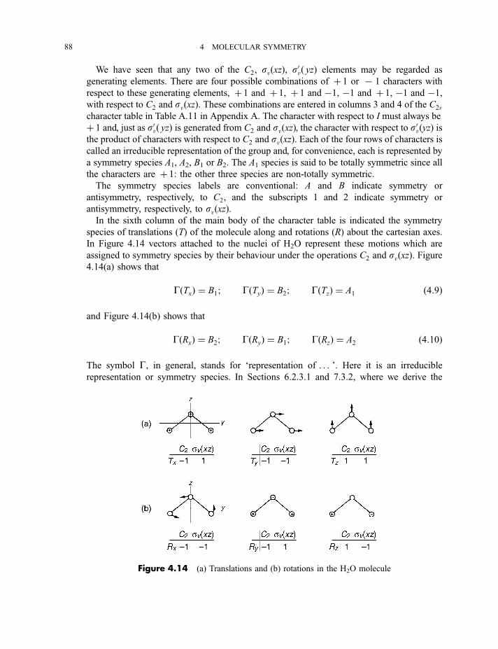
We have seen that any two of the C2, svðxzÞ, s0vð yzÞ elements may be regarded as
generating elements. There are four possible combinations of þ 1 or 7 1 characters with
respect to these generating elements, þ 1 and þ 1, þ 1 and �1, �1 and þ 1, �1 and �1,with respect to C2 and svðxzÞ. These combinations are entered in columns 3 and 4 of the C2vcharacter table in Table A.11 in Appendix A. The character with respect to I must always be
þ 1 and, just as s0vð yzÞ is generated from C2 and svðxzÞ, the character with respect to s0vðyzÞ isthe product of characters with respect to C2 and svðxzÞ. Each of the four rows of characters iscalled an irreducible representation of the group and, for convenience, each is represented by
a symmetry species A1, A2, B1 or B2. The A1 species is said to be totally symmetric since all
the characters are þ 1: the other three species are non-totally symmetric.
The symmetry species labels are conventional: A and B indicate symmetry or
antisymmetry, respectively, to C2, and the subscripts 1 and 2 indicate symmetry or
antisymmetry, respectively, to svðxzÞ.In the sixth column of the main body of the character table is indicated the symmetry
species of translations (T) of the molecule along and rotations (R) about the cartesian axes.
In Figure 4.14 vectors attached to the nuclei of H2O represent these motions which are
assigned to symmetry species by their behaviour under the operations C2 and svðxzÞ. Figure4.14(a) shows that
GðTxÞ ¼ B1; GðTyÞ ¼ B2; GðTzÞ ¼ A1 ð4:9Þ
and Figure 4.14(b) shows that
GðRxÞ ¼ B2; GðRyÞ ¼ B1; GðRzÞ ¼ A2 ð4:10Þ
The symbol G, in general, stands for ‘representation of . . . ’. Here it is an irreducible
representation or symmetry species. In Sections 6.2.3.1 and 7.3.2, where we derive the
Figure 4.14 (a) Translations and (b) rotations in the H2O molecule
88 4 MOLECULAR SYMMETRY
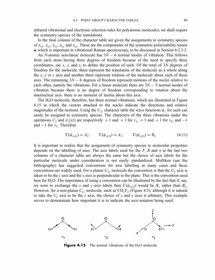
infrared vibrational and electronic selection rules for polyatomic molecules, we shall require
the symmetry species of the translations.
In the final column of the character table are given the assignments to symmetry species
of axx, ayy, axy, ayz and axz. These are the components of the symmetric polarizability tensor
a which is important in vibrational Raman spectroscopy, to be discussed in Section 6.2.3.2.
An N-atomic non-linear molecule has 3N7 6 normal modes of vibration. This follows
from each atom having three degrees of freedom because of the need to specify three
coordinates, say x, y, and z, to define the position of each. Of the total of 3N degrees of
freedom for the molecule, three represent the translation of the molecule as a whole along
the x, y or z axis and another three represent rotation of the molecule about each of these
axes. The remaining 3N7 6 degrees of freedom represent motions of the nuclei relative to
each other, namely the vibrations. For a linear molecule there are 3N7 5 normal modes of
vibration because there is no degree of freedom corresponding to rotation about the
internuclear axis: there is no moment of inertia about this axis.
The H2O molecule, therefore, has three normal vibrations, which are illustrated in Figure
4.15 in which the vectors attached to the nuclei indicate the directions and relative
magnitudes of the motions. Using the C2v character table the wave functions cv for each can
easily be assigned to symmetry species. The characters of the three vibrations under the
operations C2 and svðxzÞ are respectively þ 1 and þ 1 for n1, þ 1 and þ 1 for n2, and �1and �1 for n3. Therefore
Gðcnð1ÞÞ ¼ A1; Gðcnð2ÞÞ ¼ A1; Gðcnð3ÞÞ ¼ B2 ð4:11Þ
It is important to realize that the assignment of symmetry species to molecular properties
depends on the labelling of axes. The axis labels used for the T, R and a in the last two
columns of a character table are always the same but the choice of axis labels for the
particular molecule under consideration is not easily standardized. Mulliken (see the
bibliography) has suggested conventions for axis labelling in many cases and these
conventions are widely used. For a planar C2v molecule the convention is that the C2 axis is
taken to be the z axis and the x axis is perpendicular to the plane. This is the convention used
here for H2O. The importance of using a convention can be illustrated by the fact that if, say,
we were to exchange the x and y axis labels then Gðcnð3ÞÞ would be B1 rather than B2.
However, for a non-planar C2v molecule, such as CH2F2 (Figure 4.5), although it is natural
to take the C2 axis to be the z axis, the choice of x and y axes is arbitrary. This example
serves to demonstrate how important it is to indicate the axis notation being used.
Figure 4.15 The normal vibrations of the H2O molecule
4.3 POINT GROUP CHARACTER TABLES 89
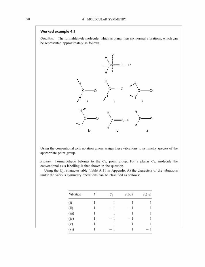
Worked example 4.1
Question. The formaldehyde molecule, which is planar, has six normal vibrations, which can
be represented approximately as follows:
Using the conventional axis notation given, assign these vibrations to symmetry species of the
appropriate point group.
Answer. Formaldehyde belongs to the C2v point group. For a planar C2v molecule the
conventional axis labelling is that shown in the question.
Using the C2v character table (Table A.11 in Appendix A) the characters of the vibrations
under the various symmetry operations can be classified as follows:
Vibration I C2 svðxzÞ s0vð yzÞ
(i) 1 1 1 1
(ii) 1 7 1 7 1 1
(iii) 1 1 1 1
(iv) 1 7 1 7 1 1
(v) 1 1 1 1
(vi) 1 7 1 1 7 1
90 4 MOLECULAR SYMMETRY
From these it follows that the symmetry species GðcvÞ of the vibrations are given by:
GðcnðiÞÞ ¼ A1
GðcnðiiÞÞ ¼ B2
GðcnðiiiÞÞ ¼ A1
GðcnðivÞÞ ¼ B2
GðcnðvÞÞ ¼ A1
GðcnðviÞÞ ¼ B1
The classifications could have been made by using any two of C2, svðxzÞ and s0vðyzÞ since anytwo of these are generating elements, and the character under I is always 1 in this point group.
Commonly used descriptions for these vibrations are: (i) symmetric CH-stretch, (ii) antisymmetricCH-stretch, (iii) CH2-scissors, (iv) CH2-rock, (v) CO-stretch, (vi) out-of-plane bend.
There will be many occasions when we shall need to multiply symmetry species or, in the
language of group theory, to obtain their direct product. For example, if H2O is vibrationally
excited simultaneously with one quantum each of n1 and n3, the symmetry species of the
wave function for this vibrational combination state is
GðcvÞ ¼ A1 � B2 ¼ B2 ð4:12Þ
In order to obtain the direct product of two species we multiply the characters under each
symmetry element using the rules
ðþ1Þ � ðþ1Þ ¼ 1; ðþ1Þ � ð�1Þ ¼ �1; ð�1Þ � ð�1Þ ¼ 1 ð4:13Þ
In this way the result in Equation (4.12) is obtained. If H2O is excited with, say, two quanta
of n3 then
GðcvÞ ¼ B2 � B2 ¼ A1 ð4:14Þ
The results of multiplication in Equations (4.12) and (4.14) for which
(a) the direct product of any species with the totally symmetric species leaves it unchanged
and
(b) the direct product of any species with itself gives the totally symmetric species
are quite general for all non-degenerate point groups.
4.3 POINT GROUP CHARACTER TABLES 91
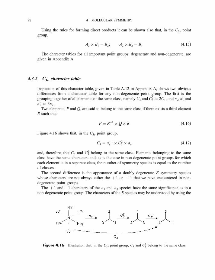
Using the rules for forming direct products it can be shown also that, in the C2v point
group,
A2 � B1 ¼ B2; A2 � B2 ¼ B1 ð4:15Þ
The character tables for all important point groups, degenerate and non-degenerate, are
given in Appendix A.
4.3.2 C3v character table
Inspection of this character table, given in Table A.12 in Appendix A, shows two obvious
differences from a character table for any non-degenerate point group. The first is the
grouping together of all elements of the same class, namely C3 and C23 as 2C3, and sv, s
0v and
s00v as 3sv.Two elements, P and Q, are said to belong to the same class if there exists a third element
R such that
P ¼ R�1 � Q� R ð4:16Þ
Figure 4.16 shows that, in the C3v point group,
C3 ¼ s�1v � C23 � sv ð4:17Þ
and, therefore, that C3 and C23 belong to the same class. Elements belonging to the same
class have the same characters and, as is the case in non-degenerate point groups for which
each element is in a separate class, the number of symmetry species is equal to the number
of classes.
The second difference is the appearance of a doubly degenerate E symmetry species
whose characters are not always either the þ 1 or 7 1 that we have encountered in non-
degenerate point groups.
The þ 1 and �1 characters of the A1 and A2 species have the same significance as in a
non-degenerate point group. The characters of the E species may be understood by using the
Figure 4.16 Illustration that, in the C3v point group, C3 and C23 belong to the same class
92 4 MOLECULAR SYMMETRY
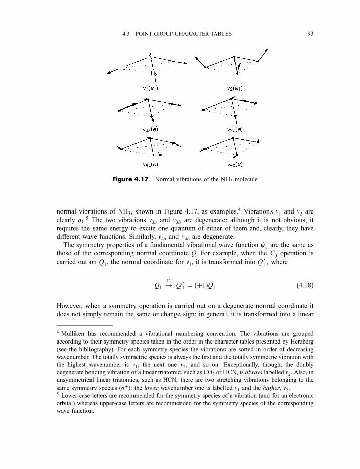
normal vibrations of NH3, shown in Figure 4.17, as examples.4 Vibrations n1 and n2 are
clearly a1.5 The two vibrations n3a and n3b are degenerate: although it is not obvious, it
requires the same energy to excite one quantum of either of them and, clearly, they have
different wave functions. Similarly, n4a and n4b are degenerate.
The symmetry properties of a fundamental vibrational wave function cv are the same as
those of the corresponding normal coordinate Q. For example, when the C3 operation is
carried out on Q1, the normal coordinate for n1, it is transformed into Q 01, where
Q1 !C3
Q 01 ¼ ðþ1ÞQ1 ð4:18Þ
However, when a symmetry operation is carried out on a degenerate normal coordinate it
does not simply remain the same or change sign: in general, it is transformed into a linear
Figure 4.17 Normal vibrations of the NH3 molecule
4 Mulliken has recommended a vibrational numbering convention. The vibrations are grouped
according to their symmetry species taken in the order in the character tables presented by Herzberg
(see the bibliography). For each symmetry species the vibrations are sorted in order of decreasing
wavenumber. The totally symmetric species is always the first and the totally symmetric vibration with
the highest wavenumber is n1, the next one n2, and so on. Exceptionally, though, the doubly
degenerate bending vibration of a linear triatomic, such as CO2 or HCN, is always labelled n2. Also, inunsymmetrical linear triatomics, such as HCN, there are two stretching vibrations belonging to the
same symmetry species (sþ): the lower wavenumber one is labelled n1 and the higher, n2.5 Lower-case letters are recommended for the symmetry species of a vibration (and for an electronic
orbital) whereas upper-case letters are recommended for the symmetry species of the corresponding
wave function.
4.3 POINT GROUP CHARACTER TABLES 93
combination of the two degenerate normal coordinates. Thus, on carrying out a symmetry
operation S,
Q3a !S
Q 03a ¼ daaQ3a þ dabQ3b
Q3b !S
Q 03b ¼ dbaQ3a þ dbbQ3b
)ð4:19Þ
In matrix notation, this can be written
Q 03aQ 03b
� �¼ daa dab
dba dbb
� �Q3a
Q3b
� �ð4:20Þ
The quantity daa þ dbb is called the trace of the matrix which is then the character of the
property, here a normal coordinate, under the symmetry operation S.
The character of the E species under the I operation is obtained from
Q3a !I
Q 03a ¼ 1� Q3a þ 0� Q3b
Q3b !I
Q 03b ¼ 0� Q3a þ 1� Q3b
)ð4:21Þ
or
Q 03aQ 03b
� �¼ 1 0
0 1
� �Q3a
Q3b
� �ð4:22Þ
The trace of the matrix is 2, which is the character of E under I.
Of the two components of n3 one, n3a, is symmetric to reflection across the sv plane
bisecting the angle between H1 and H2, and the other is antisymmetric giving
Q 03aQ 03b
� �¼ 1 0
0 �1� �
Q3a
Q3b
� �ð4:23Þ
Therefore the character of E under sv is 0. Because of the equivalence of all the sv the
character must be the same under s0v and s00v .When the operation is a rotation by an angle f about a Cn axis, in this case by an angle of
2p=3 radians about the C3 axis, the resulting coordinate transformation, a result which will
not be derived here, is given by
Q 03aQ 03b
� �¼ cosf� sinf
sinfcosf
� �Q3a
Q3b
� �ð4:24Þ
¼� 1
2
ffiffi32
q�
ffiffi32
q� 1
2
0B@
1CA Q
3a
Q3b
0@
1A
The trace of the matrix is �1 which is the character of E under C3.
94 4 MOLECULAR SYMMETRY
Except for the multiplication of E by E we follow the rules for forming direct products
used in non-degenerate point groups: the characters under the various symmetry operations
are obtained by multiplying the characters of the species being multiplied, giving
A1 � A2 ¼ A2; A2 � A2 ¼ A1; A1 � E ¼ E; A2 � E ¼ E ð4:25Þ
In multiplying E by E we use, again, examples of the vibrations of NH3. The result depends
on whether we require GðcvÞ when (a) one quantum of each of two different e vibrations is
excited (i.e. a combination level) or (b) two quanta of the same e vibration are excited (i.e. an
overtone level). In case (a), such as for the combination n3 þ n4, the product is written E � E
and the result is obtained by first squaring the characters under each operation, giving
E � E
I 2C3 3sv4 1 0
ð4:26Þ
The characters 4, 1, 0 form a reducible representation in the C3v point group and we require
to reduce it to a set of irreducible representations, the sum of whose characters under each
operation is equal to that of the reducible representation. We can express this algebraically as
wCðkÞ � wDðkÞ ¼ wFðkÞ þ wGðkÞ þ : : : ð4:27Þ
where w is a character of any operation k, and the result of multiplying the degenerate species
C and D is
C � D ¼ F þ G þ : : : ð4:28Þ
The reduction of the E � E representation, like all such reductions, gives a unique set of
irreducible representations which is
E � E ¼ A1 þ A2 þ E ð4:29Þ
We can see from Table A.12 in Appendix A that the sum of the characters of A1, A2 and E
under I, C3 and sv gives the reducible representation of Equation (4.26).
In case (b), where two quanta of the same e vibration are excited, such as 2n3, the productis written (E)2 where
ðEÞ2 ¼ A1 þ E ð4:30Þ
which is called the symmetric part of E � E, being the part which is symmetric to particle
exchange. We arrive at the result of Equation (4.30) by first obtaining the product E � E.
Then one of the species of the E � E product is forbidden. In degenerate point groups in
general this is an A species and, where possible, one which is non-totally symmetric; in this
case it is the A2 species which is forbidden and this is the antisymmetric part of E � E.
4.3 POINT GROUP CHARACTER TABLES 95
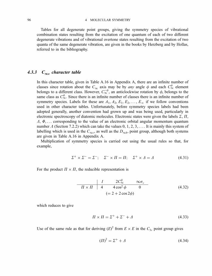
Tables for all degenerate point groups, giving the symmetry species of vibrational
combination states resulting from the excitation of one quantum of each of two different
degenerate vibrations and of vibrational overtone states resulting from the excitation of two
quanta of the same degenerate vibration, are given in the books by Herzberg and by Hollas,
referred to in the bibliography.
4.3.3 C11v character table
In this character table, given in Table A.16 in Appendix A, there are an infinite number of
classes since rotation about the C1 axis may be by any angle f and each Cf1 element
belongs to a different class. However, C�f1 , an anticlockwise rotation by f, belongs to the
same class as Cf1. Since there is an infinite number of classes there is an infinite number of
symmetry species. Labels for these are A1, A2, E1, E2, . . . , E? if we follow conventions
used in other character tables. Unfortunately, before symmetry species labels had been
adopted generally, another convention had grown up and was being used, particularly in
electronic spectroscopy of diatomic molecules. Electronic states were given the labels S, P,
D, F, . . . corresponding to the value of an electronic orbital angular momentum quantum
number L (Section 7.2.2) which can take the values 0, 1, 2, 3, . . . . It is mainly this system of
labelling which is used in the C1v, as well as the D1h, point group, although both systems
are given in Table A.16 in Appendix A.
Multiplication of symmetry species is carried out using the usual rules so that, for
example,
Sþ � S� ¼ S�; S� �P ¼ P; Sþ � D ¼ D ð4:31Þ
For the product P�P, the reducible representation is
P�P
I 2Cf1 1sv
4 4 cos2 f 0
ð¼ 2þ 2 cos 2fÞð4:32Þ
which reduces to give
P�P ¼ Sþ þ S� þ D ð4:33Þ
Use of the same rule as that for deriving (E)2 from E � E in the C3v point group gives
ðPÞ2 ¼ Sþ þ D ð4:34Þ
96 4 MOLECULAR SYMMETRY
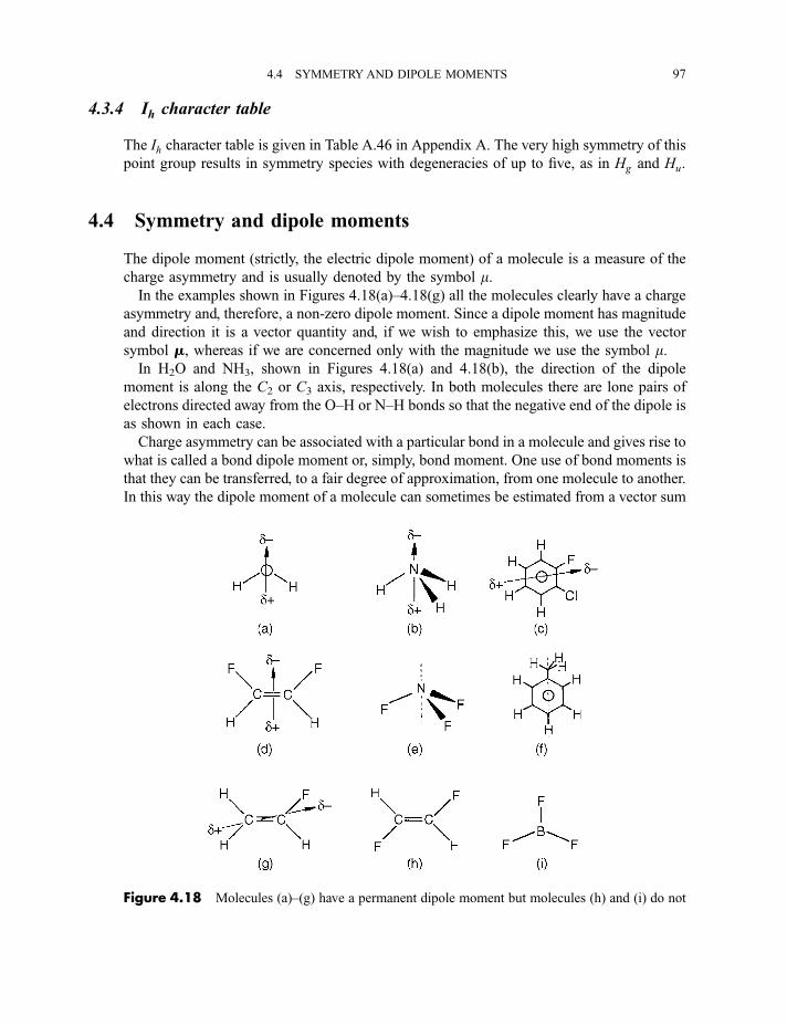
4.3.4 Ih character table
The Ih character table is given in Table A.46 in Appendix A. The very high symmetry of this
point group results in symmetry species with degeneracies of up to five, as in Hg and Hu.
4.4 Symmetry and dipole moments
The dipole moment (strictly, the electric dipole moment) of a molecule is a measure of the
charge asymmetry and is usually denoted by the symbol m.In the examples shown in Figures 4.18(a)–4.18(g) all the molecules clearly have a charge
asymmetry and, therefore, a non-zero dipole moment. Since a dipole moment has magnitude
and direction it is a vector quantity and, if we wish to emphasize this, we use the vector
symbol m, whereas if we are concerned only with the magnitude we use the symbol m.In H2O and NH3, shown in Figures 4.18(a) and 4.18(b), the direction of the dipole
moment is along the C2 or C3 axis, respectively. In both molecules there are lone pairs of
electrons directed away from the O–H or N–H bonds so that the negative end of the dipole is
as shown in each case.
Charge asymmetry can be associated with a particular bond in a molecule and gives rise to
what is called a bond dipole moment or, simply, bond moment. One use of bond moments is
that they can be transferred, to a fair degree of approximation, from one molecule to another.
In this way the dipole moment of a molecule can sometimes be estimated from a vector sum
Figure 4.18 Molecules (a)–(g) have a permanent dipole moment but molecules (h) and (i) do not
4.4 SYMMETRY AND DIPOLE MOMENTS 97
of bond moments. For example, the dipole moment of 2-chlorofluorobenzene, shown in
Figure 4.18(c), can be estimated from the vector sum of the C–F and C–Cl bond moments
found from, say, CH3F and CH3Cl, respectively.
Bond moments for bonds involving a hydrogen atom are relatively small, so that the
dipole moments of H2O and NH3 are dominated by the effects of the lone pairs of electrons.
The dipole moment of cis-1,2-difluoroethylene, shown in Figure 4.18(d), is dominated by
the large bond moments of the C–F bonds, and the negative ends are directed towards the
fluorine atoms because of the high electronegativity of fluorine. The dipole moment is
directed along the C2 axis, with the negative end as shown.
In NF3 and C6H5CH3 (toluene), shown in Figures 4.18(e) and 4.18(f ), respectively, charge
asymmetry confers a dipole moment on both molecules in the directions shown by the
dotted lines, but it is not obvious which is the negative end. In NF3 the effect of the
electronegative fluorine atoms tends to be counterbalanced by the lone pair of electrons on
the nitrogen atom, and in C6H5CH3 all the C–H bond moments are very small and their
vector sum is not a reliable indicator of which is the negative end of the dipole. Both
molecules have very small dipole moments.
The magnitude m of a dipole moment is usually quoted in Debye units. Dipole moments
are products of charges and their separations so that, for charges of �q and þq separated by
a distance r,
m ¼ qr ð4:35ÞFor a molecule with many nuclei and electrons with charges qi
mm ¼Pi
qiri ð4:36Þ
Equations (4.35) and (4.36) show that the SI unit of dipole moment is the product of the SI
units of charge and distance, which are the coulomb and the metre, respectively. However,
the unit of C m is a rather cumbersome one, and the old unit of the Debye (D) is still
commonly used for the reason that molecular dipole moments are conveniently of the order
of 1 D. The units are related by
1 D ’ 3:335 64� 10�30 C m ð4:37ÞQuantitatively, using the Debye unit, the dipole moments of NH3 (1.47 D), NF3 (0.2 D) and
C6H5CH3 (0.36 D) confirm the simple arguments which we have made about their
magnitudes.
It is important to realize that, although various types of experiments can give the value of
a dipole moment, none is capable of determining the direction in which the negative or
positive end lies. In molecules such as NF3 and C6H5CH3, in which the dipole moment is so
small that simple arguments will not predict the direction, only accurate valence theory
calculations can provide the answer. These calculations themselves are reliable only for
fairly small molecules (see Section 5.2.3 for the case of CO).
The large C–F bond moment in fluoroethylene, shown in Figure 4.18(g), dominates the
dipole moment, which must lie in the molecular plane, but its direction in that plane will
depend on the effects of the other parts of the molecule with the result that it will not lie
exactly along the C–F bond.
98 4 MOLECULAR SYMMETRY
In molecules such as trans-1,2-difluoroethylene and BF3, illustrated in Figures 4.18(h)
and 4.18(i), respectively, it may be obvious at this stage that their dipole moments are zero,
but we shall see later that symmetry arguments confirm that this is so.
Looking at all the examples in Figure 4.18 suggests that molecular symmetry can be used
to formulate a rule which will tell us whether any molecule has a non-zero dipole moment.
The dipole moment vector mm must be totally symmetric, and therefore symmetric to all
operations of the point group to which the molecule belongs: otherwise the direction of the
dipole moment could be reversed by carrying out a symmetry operation, and this clearly
cannot happen. The vector mm has components mx, my and mz along the cartesian axes of the
molecule. In the examples of NH3 and NF3, shown in Figures 4.18(b) and 4.18(e),
respectively, if the C3 axis is the z-axis, mz 6¼ 0 but mx ¼ my ¼ 0. Similarly in H2O and cis-
1,2-difluoroethylene, shown in Figures 4.18(a) and 4.18(d), respectively, if the C2 axis is the
z-axis mz 6¼ 0 but mx ¼ my ¼ 0. In the case of fluoroethylene, shown in Figure 4.18(g), if the
molecular plane is the xy-plane, then mx 6¼ 0 and my 6¼ 0 but mz ¼ 0. In a molecule such as
CHFClBr, shown in Figure 4.7, the dipole moment is not confined by symmetry in any way
so that mx 6¼ 0, my 6¼ 0 and mz 6¼ 0.
If we compare the vectors representing a translation of, say, the H2O molecule along the
z-axis, as illustrated in Figure 4.14(a), with the dipole moment vector, which is also along
the z-axis and shown in Figure 4.18(a), it is clear that they have the same symmetry species
[i.e. GðmzÞ ¼ GðTzÞ] and, in general,
GðmxÞ ¼ GðTxÞGðmyÞ ¼ GðTyÞGðmzÞ ¼ GðTzÞ
9=; ð4:38Þ
for all molecules. Because mm must be totally symmetric, a molecule has a permanent dipole
moment if any of the components mx, my or mz is totally symmetric. With the relationships in
Equations (4.38) we can formulate the general rule:
A molecule has a permanent dipole moment if any of the translational symmetry species
of the point group to which the molecule belongs is totally symmetric.
Then, if we look through all the point group character tables in Appendix A to see if any of
the translational symmetry species is totally symmetric, it is apparent that molecules
belonging to only the following point groups have a permanent dipole moment:
(a) C1, in which GðTxÞ ¼ GðTyÞ ¼ GðTzÞ ¼ A;
(b) Cs, in which GðTxÞ ¼ GðTyÞ ¼ A0;
(c) Cn, in which GðTzÞ ¼ A;
(d) Cnv, in which GðTzÞ ¼ A1 (or Sþ in C1v).
In the C1, Cs, Cn and Cnv point groups the totally symmetric symmetry species is A, A0, Aand A1 (or Sþ), respectively. For example, CHFClBr (Figure 4.7) belongs to the C1 point
group: therefore m 6¼ 0 and, since all three translations are totally symmetric, the dipole
4.4 SYMMETRY AND DIPOLE MOMENTS 99
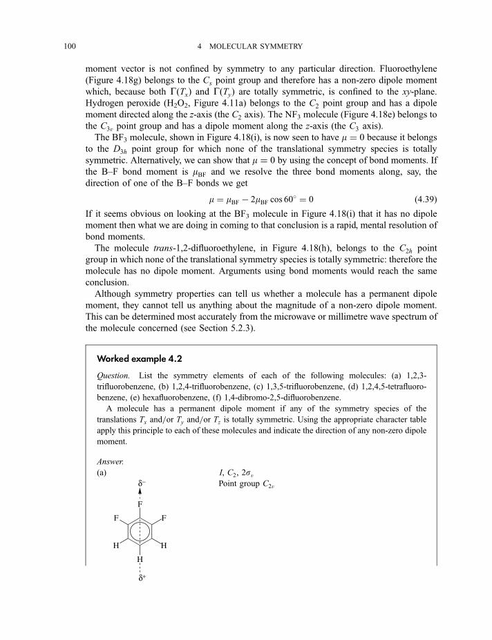
moment vector is not confined by symmetry to any particular direction. Fluoroethylene
(Figure 4.18g) belongs to the Cs point group and therefore has a non-zero dipole moment
which, because both GðTxÞ and GðTyÞ are totally symmetric, is confined to the xy-plane.
Hydrogen peroxide (H2O2, Figure 4.11a) belongs to the C2 point group and has a dipole
moment directed along the z-axis (the C2 axis). The NF3 molecule (Figure 4.18e) belongs to
the C3v point group and has a dipole moment along the z-axis (the C3 axis).
The BF3 molecule, shown in Figure 4.18(i), is now seen to have m ¼ 0 because it belongs
to the D3h point group for which none of the translational symmetry species is totally
symmetric. Alternatively, we can show that m ¼ 0 by using the concept of bond moments. If
the B–F bond moment is mBF and we resolve the three bond moments along, say, the
direction of one of the B–F bonds we get
m ¼ mBF � 2mBF cos 60� ¼ 0 ð4:39Þ
If it seems obvious on looking at the BF3 molecule in Figure 4.18(i) that it has no dipole
moment then what we are doing in coming to that conclusion is a rapid, mental resolution of
bond moments.
The molecule trans-1,2-difluoroethylene, in Figure 4.18(h), belongs to the C2h point
group in which none of the translational symmetry species is totally symmetric: therefore the
molecule has no dipole moment. Arguments using bond moments would reach the same
conclusion.
Although symmetry properties can tell us whether a molecule has a permanent dipole
moment, they cannot tell us anything about the magnitude of a non-zero dipole moment.
This can be determined most accurately from the microwave or millimetre wave spectrum of
the molecule concerned (see Section 5.2.3).
Worked example 4.2
Question. List the symmetry elements of each of the following molecules: (a) 1,2,3-
trifluorobenzene, (b) 1,2,4-trifluorobenzene, (c) 1,3,5-trifluorobenzene, (d) 1,2,4,5-tetrafluoro-
benzene, (e) hexafluorobenzene, (f) 1,4-dibromo-2,5-difluorobenzene.
A molecule has a permanent dipole moment if any of the symmetry species of the
translations Tx and=or Ty and=or Tz is totally symmetric. Using the appropriate character table
apply this principle to each of these molecules and indicate the direction of any non-zero dipole
moment.
Answer.
(a) I, C2, 2svPoint group C2v
F
FF
H
H
H
δ−
δ+
100 4 MOLECULAR SYMMETRY
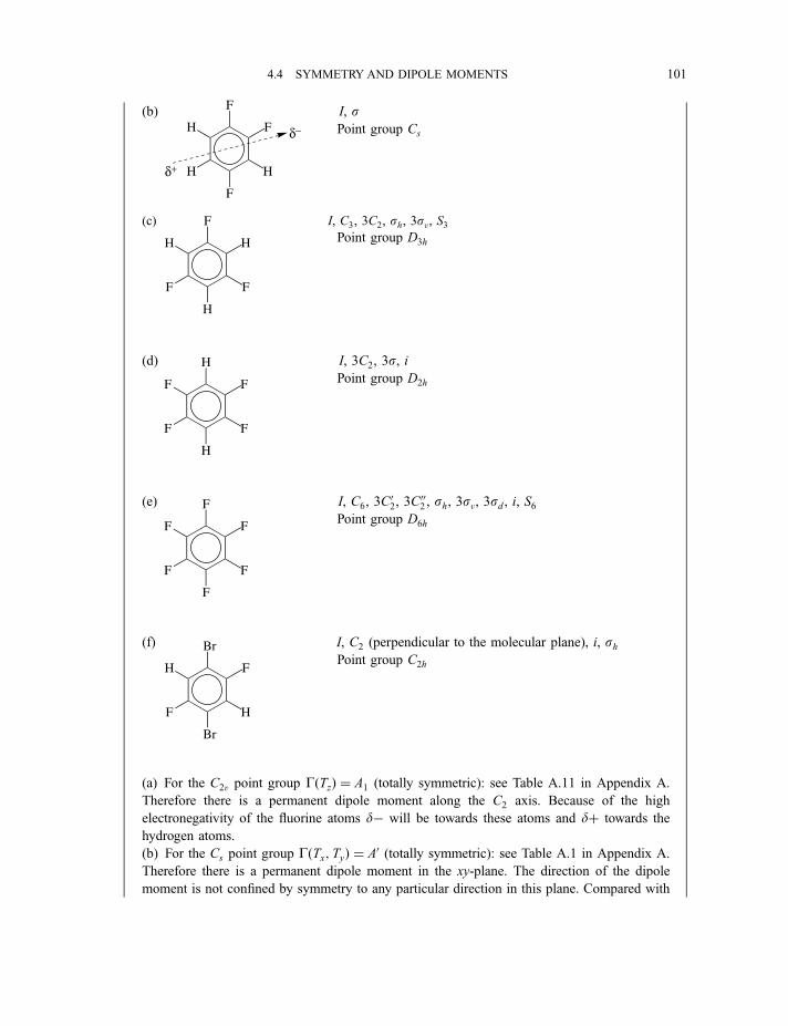
(b) I, sPoint group Cs
(c) I, C3, 3C2, sh, 3sv, S3Point group D3h
(d) I, 3C2, 3s, iPoint group D2h
(e) I, C6, 3C02, 3C
002 , sh, 3sv, 3sd , i, S6
Point group D6h
(f) I, C2 (perpendicular to the molecular plane), i, shPoint group C2h
(a) For the C2v point group GðTzÞ ¼ A1 (totally symmetric): see Table A.11 in Appendix A.
Therefore there is a permanent dipole moment along the C2 axis. Because of the high
electronegativity of the fluorine atoms d� will be towards these atoms and dþ towards the
hydrogen atoms.
(b) For the Cs point group GðTx; TyÞ ¼ A0 (totally symmetric): see Table A.1 in Appendix A.
Therefore there is a permanent dipole moment in the xy-plane. The direction of the dipole
moment is not confined by symmetry to any particular direction in this plane. Compared with
F
FH
H
F
H
δ−
δ+
F
H
F
H
F
H
H
F
F
F
F
H
F
F
F
F
F
F
Br
H
F
F
H
Br
4.4 SYMMETRY AND DIPOLE MOMENTS 101
1,2,3-trifluorobenzene the shift of a fluorine atom from position 3 to 4 will tilt the dipole
moment towards position 4.The other four molecules, (c)–(f ), do not have permanent dipole moments, as inspection of the
relevant character tables in Appendix A will confirm.
Exercises
4.1 The following molecules, in going from the ground to an excited electronic state,
undergo a change of geometry which involves a change of point group:
(a) ammonia (pyramidal ground state, planar excited state);
(b) acetylene (linear ground state, trans bent excited state);
(c) fluoroacetylene (linear ground state, trans bent excited state);
(d) formaldehyde (planar ground state, pyramidal excited state).
List the symmetry elements and point groups of these molecules in both electronic
states.
4.2 List all the symmetry elements of the following molecules, assign each to a point
group, and state whether they form enantiomers: (a) lactic acid, (b) trans-
[Co(ethylenediamine)2Cl2]þ, (c) cis-[Co(ethylenediamine)2Cl2]
þ, (d) cyclopropane,
(e) trans-1,2-dichlorocyclopropane, (f) 1-chloro-3-fluoroallene.
4.3 Assign the allene molecule to a point group and use the character table to form the
direct products A2 � B1, B1 � B2, B2 � E and E � E. Show how the symmetry species
of the point group to which 1,1-difluoroallene belongs correlate with those of allene.
Bibliography
Bunker, P. R. and Jensen, P. (1998) Molecular Symmetry and Spectroscopy, 2nd edn., NRC Press,
Canada.
Cotton, F. A. (1971) Chemical Applications of Group Theory, John Wiley, New York.
Davidson, G. (1991) Group Theory for Chemists, Macmillan, London.
Herzberg, G. (1991) Infrared and Raman Spectra of Polyatomic Molecules, Krieger, Florida.
Hollas, J. M. (1972) Symmetry in Molecules, Chapman and Hall, London.
Mulliken, R. S. (1955) J. Chem. Phys., 23, 1997.
Ogden, J. S. (2001) Introduction to Molecular Symmetry, Oxford University Press, Oxford.
Schonland, D. (1965) Molecular Symmetry, Van Nostrand, London.
Vincent, A. (2000) Molecular Symmetry and Group Theory, 2nd edn., John Wiley, Chichester.
102 4 MOLECULAR SYMMETRY
5Rotational Spectroscopy
5.1 Linear, symmetric rotor, spherical rotor and asymmetricrotor molecules
For the purposes of studying the rotational spectra of molecules it is essential to classify
them according to their principal moments of inertia.
The moment of inertia I of any molecule about any axis through the centre of gravity is
given by
I ¼Pi
mir2i ð5:1Þ
where mi and ri are the mass and distance of atom i from the axis. There is one of these axes,
conventionally labelled the c axis, about which the moment of inertia has its maximum value
and a second axis, labelled the a axis, about which the moment of inertia has its minimum
value. It can be shown that the a and c axes must be mutually perpendicular. These, together
with a third axis, the b axis, which is perpendicular to the other two, are called the principal
axes of inertia and the corresponding moments of inertia Ia, Ib and Ic are the principal
moments of inertia. In general, according to convention,
Ic 5 Ib 5 Ia ð5:2Þ
For a linear molecule, such as HCN in Figure 5.1(a),
Ic ¼ Ib > Ia ¼ 0 ð5:3Þ
where the b and c axes may be in any direction perpendicular to the internuclear a axis.
Considering the nuclei as point masses on the a axis, it is clear that Ia must be zero, since all
the ri in Equation (5.1) are zero.
For a symmetric rotor, or symmetric top as it is sometimes called, two of the principal
moments of inertia are equal and the third is non-zero. If
Ic ¼ Ib > Ia ð5:4Þ
the molecule is a prolate symmetric rotor. Figure 5.1(b) shows the example of methyl iodide.
Since the heavy iodine nucleus makes no contribution to Ia, which is therefore relatively
103
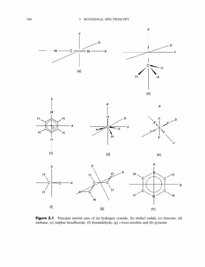
Figure 5.1 Principal inertial axes of (a) hydrogen cyanide, (b) methyl iodide, (c) benzene, (d)
methane, (e) sulphur hexafluoride, (f) formaldehyde, (g) s-trans-acrolein and (h) pyrazine
104 5 ROTATIONAL SPECTROSCOPY
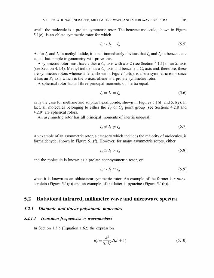
small, the molecule is a prolate symmetric rotor. The benzene molecule, shown in Figure
5.1(c), is an oblate symmetric rotor for which
Ic > Ib ¼ Ia ð5:5Þ
As for Ic and Ib in methyl iodide, it is not immediately obvious that Ib and Ia in benzene are
equal, but simple trigonometry will prove this.
A symmetric rotor must have either a Cn axis with n> 2 (see Section 4.1.1) or an S4 axis
(see Section 4.1.4). Methyl iodide has a C3 axis and benzene a C6 axis and, therefore, these
are symmetric rotors whereas allene, shown in Figure 4.3(d), is also a symmetric rotor since
it has an S4 axis which is the a axis: allene is a prolate symmetric rotor.
A spherical rotor has all three principal moments of inertia equal:
Ic ¼ Ib ¼ Ia ð5:6Þ
as is the case for methane and sulphur hexafluoride, shown in Figures 5.1(d) and 5.1(e). In
fact, all molecules belonging to either the Td or Oh point group (see Sections 4.2.8 and
4.2.9) are spherical rotors.
An asymmetric rotor has all principal moments of inertia unequal:
Ic 6¼ Ib 6¼ Ia ð5:7Þ
An example of an asymmetric rotor, a category which includes the majority of molecules, is
formaldehyde, shown in Figure 5.1(f). However, for many asymmetric rotors, either
Ic ’ Ib > Ia ð5:8Þ
and the molecule is known as a prolate near-symmetric rotor, or
Ic > Ib ’ Ia ð5:9Þ
when it is known as an oblate near-symmetric rotor. An example of the former is s-trans-
acrolein (Figure 5.1(g)) and an example of the latter is pyrazine (Figure 5.1(h)).
5.2 Rotational infrared, millimetre wave and microwave spectra
5.2.1 Diatomic and linear polyatomic molecules
5.2.1.1 Transition frequencies or wavenumbers
In Section 1.3.5 (Equation 1.62) the expression
Er ¼h2
8p2IJ ðJ þ 1Þ ð5:10Þ
5.2 ROTATIONAL INFRARED, MILLIMETRE WAVE AND MICROWAVE SPECTRA 105

for the rotational energy levels Er of a diatomic molecule, in the rigid rotor approximation,
was introduced. In this equation, I is the moment of inertia [equal to mr2, where the reducedmass m is equal to m1m2=ðm1 þ m2Þ� and the rotational quantum number J ¼ 0; 1; 2; . . . .The same expression applies also to any linear polyatomic molecule but, because I is likely
to be larger than for a diatomic molecule, the energy levels of Figure 1.12 tend to be more
closely spaced.
In practice, what is measured experimentally is not energy but frequency, in the millimetre
wave and microwave regions, or wavenumber, in the far infrared. Therefore we convert the
energy levels of Equation (5.10) to what are known as term values FðJ Þ having dimensions
of either frequency, by dividing by h, or wavenumber, by dividing by hc, giving
FðJ Þ ¼ Er
h¼ h
8p2IJ ðJ þ 1Þ ¼ BJ ðJ þ 1Þ ð5:11Þ
or
FðJ Þ ¼ Er
hc¼ h
8p2cIJ ðJ þ 1Þ ¼ BJ ðJ þ 1Þ ð5:12Þ
The use of the symbols FðJ Þ and B for quantities which may have dimensions of frequency
or wavenumber is unfortunate, but the symbolism is used so commonly that there seems
little prospect of change. In Equations (5.11) and (5.12) the quantity B is known as the
rotational constant. Its determination by spectroscopic means results in determination of
internuclear distances and represents a very powerful structural technique.
Figure 5.2 shows a set of rotational energy levels, or, strictly, term values, for the CO
molecule.
The transition intensity is proportional to the square of the transition moment, which is
given by
Rr ¼ðc0r*mmc
00r dt ð5:13Þ
analogous to Equation (2.13). The rotational selection rules constitute the conditions for
which the intensity, and therefore Rr, is non-zero and are:
1. The molecule must have a permanent dipole moment (m 6¼ 0).
2. DJ ¼ �1.3. DMJ ¼ 0, �1, a rule which is important only if the molecule is in an electric or magnetic
field (see Equation 1.61).
Rule 1 shows that transitions are allowed in heteronuclear diatomic molecules such as CO,
NO, HF and even 1H2H (for which m ¼ 5:9� 10�4 D compared with, say, HF, for which
m ¼ 1.82 D),1 but not in H2, Cl2 and N2. Similarly, ‘unsymmetrical’ linear polyatomic
1 1 D’ 3.335 646 10730 C m.
106 5 ROTATIONAL SPECTROSCOPY
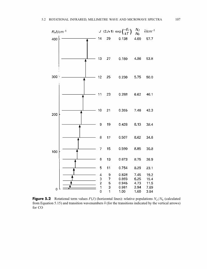
Figure 5.2 Rotational term values FðJ Þ (horizontal lines): relative populations NJ=N0 (calculated
from Equation 5.15) and transition wavenumbers ~nn (for the transitions indicated by the vertical arrows)for CO
5.2 ROTATIONAL INFRARED, MILLIMETRE WAVE AND MICROWAVE SPECTRA 107
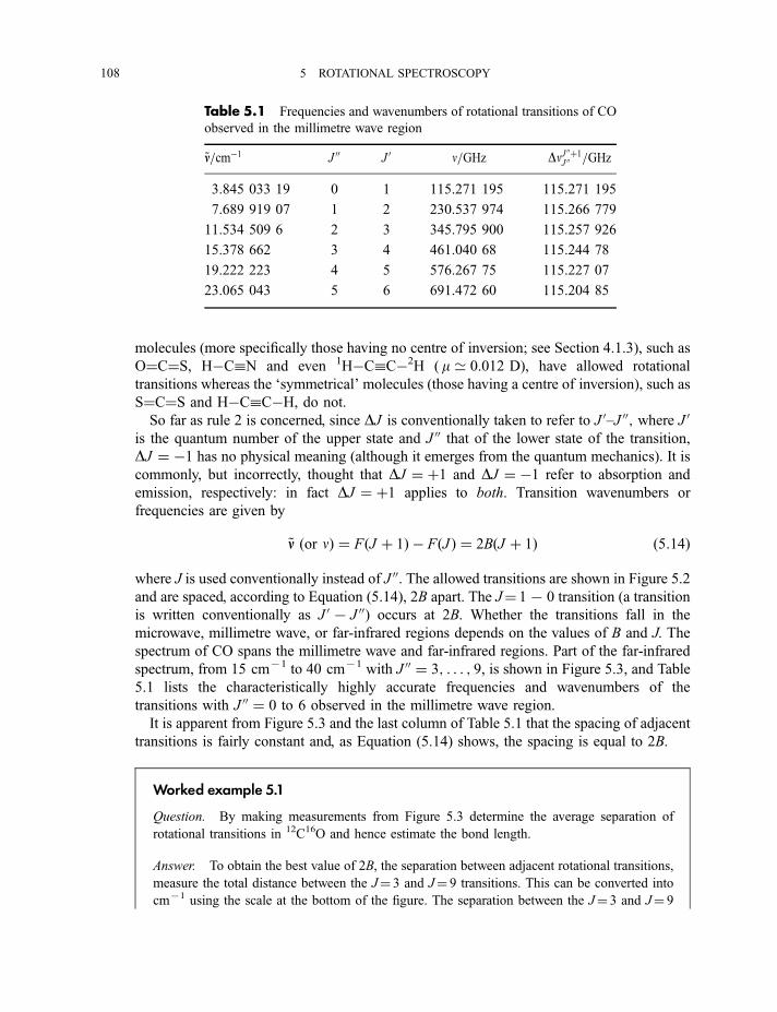
molecules (more specifically those having no centre of inversion; see Section 4.1.3), such as
O¼C¼S, H�CN and even 1H�CC�2H ( m ’ 0.012 D), have allowed rotational
transitions whereas the ‘symmetrical’ molecules (those having a centre of inversion), such as
S¼C¼S and H�CC�H, do not.
So far as rule 2 is concerned, since DJ is conventionally taken to refer to J 0–J 00; where J 0
is the quantum number of the upper state and J 00 that of the lower state of the transition,
DJ ¼ �1 has no physical meaning (although it emerges from the quantum mechanics). It is
commonly, but incorrectly, thought that DJ ¼ þ1 and DJ ¼ �1 refer to absorption and
emission, respectively: in fact DJ ¼ þ1 applies to both. Transition wavenumbers or
frequencies are given by
~nn ðor nÞ ¼ FðJ þ 1Þ � FðJ Þ ¼ 2BðJ þ 1Þ ð5:14Þ
where J is used conventionally instead of J 00. The allowed transitions are shown in Figure 5.2and are spaced, according to Equation (5.14), 2B apart. The J¼ 17 0 transition (a transition
is written conventionally as J 07 J 00) occurs at 2B. Whether the transitions fall in the
microwave, millimetre wave, or far-infrared regions depends on the values of B and J. The
spectrum of CO spans the millimetre wave and far-infrared regions. Part of the far-infrared
spectrum, from 15 cm71 to 40 cm71 with J 00 ¼ 3; . . . ; 9, is shown in Figure 5.3, and Table
5.1 lists the characteristically highly accurate frequencies and wavenumbers of the
transitions with J 00 ¼ 0 to 6 observed in the millimetre wave region.
It is apparent from Figure 5.3 and the last column of Table 5.1 that the spacing of adjacent
transitions is fairly constant and, as Equation (5.14) shows, the spacing is equal to 2B.
Worked example 5.1
Question. By making measurements from Figure 5.3 determine the average separation of
rotational transitions in 12C16O and hence estimate the bond length.
Answer. To obtain the best value of 2B, the separation between adjacent rotational transitions,
measure the total distance between the J¼ 3 and J¼ 9 transitions. This can be converted into
cm71 using the scale at the bottom of the figure. The separation between the J¼ 3 and J¼ 9
Table 5.1 Frequencies and wavenumbers of rotational transitions of CO
observed in the millimetre wave region
~nn=cm�1 J 00 J 0 n=GHz DnJ00þ1
J 00 =GHz
3.845 033 19 0 1 115.271 195 115.271 195
7.689 919 07 1 2 230.537 974 115.266 779
11.534 509 6 2 3 345.795 900 115.257 926
15.378 662 3 4 461.040 68 115.244 78
19.222 223 4 5 576.267 75 115.227 07
23.065 043 5 6 691.472 60 115.204 85
108 5 ROTATIONAL SPECTROSCOPY
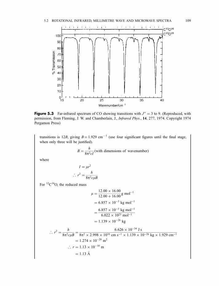
transitions is 12B, giving B¼ 1.929 cm71 (use four significant figures until the final stage,
when only three will be justified).
B ¼ h
8p2cIðwith dimensions of wavenumberÞ
where
I ¼ mr2
; r2 ¼ h
8p2cmB
For 12C16O, the reduced mass
m ¼ 12:00� 16:00
12:00þ 16:00g mol�1
¼ 6:857� 10�3 kg mol�1
¼ 6:857� 10�3 kg mol�1
6:022� 1023 mol�1
¼ 1:139� 10�26 kg
; r2 ¼ h
8p2cmB¼ 6:626� 10�34 J s
8p2 � 2:998� 1010 cm s�1 � 1:139� 10�26 kg� 1:929 cm�1
¼ 1:274� 10�20 m2
; r ¼ 1:13� 10�10 m
¼ 1:13 A�
Figure 5.3 Far-infrared spectrum of CO showing transitions with J 00 ¼ 3 to 9. (Reproduced, with
permission, from Fleming, J. W. and Chamberlain, J., Infrared Phys., 14, 277, 1974. Copyright 1974
Pergamon Press)
5.2 ROTATIONAL INFRARED, MILLIMETRE WAVE AND MICROWAVE SPECTRA 109
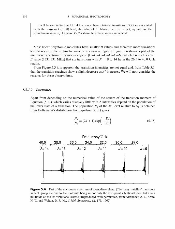
It will be seen in Section 5.2.1.4 that, since these rotational transitions of CO are associated
with the zero-point (v¼ 0) level, the value of B obtained here is, in fact, B0 and not the
equilibrium value Be. Equation (5.25) shows how these values are related.
Most linear polyatomic molecules have smaller B values and therefore more transitions
tend to occur in the millimetre wave or microwave regions. Figure 5.4 shows a part of the
microwave spectrum of cyanodiacetylene (H�CC�CC�CN) which has such a small
B value (1331.331 MHz) that six transitions with J 00 ¼ 9 to 14 lie in the 26.5 to 40.0 GHz
region.
From Figure 5.3 it is apparent that transition intensities are not equal and, from Table 5.1,
that the transition spacings show a slight decrease as J 00 increases. We will now consider the
reasons for these observations.
5.2.1.2 Intensities
Apart from depending on the numerical value of the square of the transition moment of
Equation (5.13), which varies relatively little with J, intensities depend on the population of
the lower state of a transition. The population NJ of the Jth level relative to N0 is obtained
from Boltzmann’s distribution law. Equation (2.11) gives
NJ
N0
¼ ð2J þ 1Þ exp � Er
kT
� �ð5:15Þ
Figure 5.4 Part of the microwave spectrum of cyanodiacetylene. (The many ‘satellite’ transitions
in each group are due to the molecule being in not only the zero-point vibrational state but also a
multitude of excited vibrational states.) (Reproduced, with permission, from Alexander, A. J., Kroto,
H. W. and Walton, D. R. M., J. Mol. Spectrosc., 62, 175, 1967)
110 5 ROTATIONAL SPECTROSCOPY
where ð2J þ 1Þ is the degeneracy of the J th level. This degeneracy arises from the fact that,
in the absence of an electric or magnetic field, ð2J þ 1Þ levels, resulting from the number of
values that MJ (see Equation 1.61) can take, are all of the same energy: in other words they
are degenerate. Values of ð2J þ 1Þ, expð�Er=kT Þ and NJ=N0 are given for CO in Figure 5.2
and illustrate the point that there are two opposing factors in NJ=N0. The ð2J þ 1Þ factorincreases with J whereas the expð�Er=kT Þ factor decreases rapidly, so that NJ=N0 increases
at low J until, at higher J, the exponential factor wins and NJ=N0 approaches zero. The
population therefore shows a maximum at a value of J ¼ Jmax corresponding to
dðNJ=N0ÞdJ
¼ 0 ð5:16Þ
which gives
Jmax ¼kT
2hB
� �1=2
� 1
2ð5:17Þ
for B having dimensions of frequency. Figure 5.2 shows that Jmax¼ 7 for CO. In fact, Figure
5.3 shows that the observed maximum intensity is at about J 00 ¼ 8 because there are other,
less important, factors that we have neglected.
5.2.1.3 Centrifugal distortion
The small decrease in transition spacings with increasing J, as shown for example in Table
5.1, compared with the constant spacings we expected is due to our original approximation
in Section 1.3.5 of treating the molecule as a rigid rotor being not quite valid. In fact the
bond is not rigid but is more accurately represented by a spring connecting the nuclei, as was
apparent when we considered vibrational motion in Section 1.3.6. So it is not surprising that,
as the speed of rotation increases (i.e. as J increases), the nuclei tend to be thrown outwards
by centrifugal forces. The spring stretches, r increases and, therefore, B decreases.
Originally, this J-dependent decrease of B was included by changing the term values of
Equations (5.11) and (5.12) to
FðJ Þ ¼ B½1� uJ ðJ þ 1Þ� J ðJ þ 1Þ ð5:18Þ
where u is an additional constant, but it is usually written in the form
FðJ Þ ¼ BJ ðJ þ 1Þ � DJ 2ðJ þ 1Þ2 ð5:19Þ
where D is the centrifugal distortion constant and is always positive for diatomic molecules.
The transition wavenumbers or frequencies are now modified from Equation (5.14) to
~nn ðor nÞ ¼ FðJ þ 1Þ � FðJ Þ ¼ 2BðJ þ 1Þ � 4DðJ þ 1Þ3 ð5:20Þ
5.2 ROTATIONAL INFRARED, MILLIMETRE WAVE AND MICROWAVE SPECTRA 111
The centrifugal distortion constant depends on the stiffness of the bond and it is not
surprising that it can be related to the vibration wavenumber o, in the harmonic
approximation (see Section 1.3.6), by
D ¼ 4B3
o2ð5:21Þ
5.2.1.4 Diatomic molecules in excited vibrational states
There is a stack of rotational levels, with term values such as those given by Equation (5.19),
associated with not only the zero-point vibrational level but also all the other vibrational
levels shown, for example, in Figure 1.13. However, the Boltzmann equation (Equation
2.11), together with the vibrational energy level expression (Equation 1.69), gives the ratio
of the population Nv of the vth vibrational level to N0, that of the zero-point level, as
Nv
N0
¼ exp � hcvokT
� �ð5:22Þ
where o is the vibration wavenumber and v the vibrational quantum number. Since this ratio
is, for example, only 0.10 for v¼ 1 and o¼ 470 cm71 we can see that rotational transitions
in excited vibrational states are generally very weak unless either the molecule is particularly
heavy, leading to a relatively small value of o, or the temperature is high; however, the
negative exponential nature of Equation (5.22) means that increasing the temperature has
only quite a small effect on populations.
The rotational constants B and D are both slightly vibrationally dependent so that the term
values of Equation (5.19) should be written
FvðJ Þ ¼ Bv J ðJ þ 1Þ � Dv J2ðJ þ 1Þ2 ð5:23Þ
and Equation (5.20) becomes
~nn ðor nÞ ¼ 2BvðJ þ 1Þ � 4DvðJ þ 1Þ3 ð5:24Þ
The vibrational dependence of B is given, to a good approximation, by
Bv ¼ Be � aðvþ 12Þ ð5:25Þ
where Be refers to the hypothetical equilibrium state of the molecule at the bottom of the
potential energy curve of Figure 1.13 and a is a vibration–rotation interaction constant. In
order to obtain Be, and hence the equilibrium bond length re, Bv must be obtained in at least
two vibrational states. If there is insufficient population of the v¼ 1 level to obtain B1 then
rotational spectroscopy can give only B0.
112 5 ROTATIONAL SPECTROSCOPY
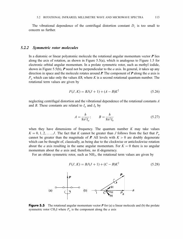
The vibrational dependence of the centrifugal distortion constant Dv is too small to
concern us further.
5.2.2 Symmetric rotor molecules
In a diatomic or linear polyatomic molecule the rotational angular momentum vector P lies
along the axis of rotation, as shown in Figure 5.5(a), which is analogous to Figure 1.5 for
electronic orbital angular momentum. In a prolate symmetric rotor, such as methyl iodide,
shown in Figure 5.5(b), P need not be perpendicular to the a axis. In general, it takes up any
direction in space and the molecule rotates around P. The component of P along the a axis is
Pa which can take only the values Kh, where K is a second rotational quantum number. The
rotational term values are given by
FðJ ;KÞ ¼ BJ ðJ þ 1Þ þ ðA� BÞK2 ð5:26Þ
neglecting centrifugal distortion and the vibrational dependence of the rotational constants A
and B. These constants are related to Ia and Ib by
A ¼ h
8p2Ia; B ¼ h
8p2Ibð5:27Þ
when they have dimensions of frequency. The quantum number K may take values
K ¼ 0; 1; 2; . . . ; J . The fact that K cannot be greater than J follows from the fact that Pa
cannot be greater than the magnitude of P. All levels with K > 0 are doubly degenerate
which can be thought of, classically, as being due to the clockwise or anticlockwise rotation
about the a axis resulting in the same angular momentum. For K ¼ 0 there is no angular
momentum about the a axis and, therefore, no K-degeneracy.
For an oblate symmetric rotor, such as NH3, the rotational term values are given by
FðJ ;KÞ ¼ BJ ðJ þ 1Þ þ ðC � BÞK2 ð5:28Þ
Figure 5.5 The rotational angular momentum vector P for (a) a linear molecule and (b) the prolate
symmetric rotor CH3I where Pa is the component along the a axis
5.2 ROTATIONAL INFRARED, MILLIMETRE WAVE AND MICROWAVE SPECTRA 113
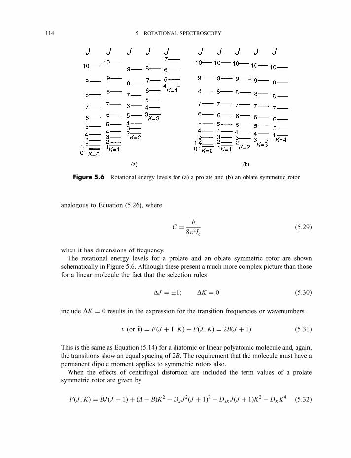
analogous to Equation (5.26), where
C ¼ h
8p2Icð5:29Þ
when it has dimensions of frequency.
The rotational energy levels for a prolate and an oblate symmetric rotor are shown
schematically in Figure 5.6. Although these present a much more complex picture than those
for a linear molecule the fact that the selection rules
DJ ¼ �1; DK ¼ 0 ð5:30Þ
include DK ¼ 0 results in the expression for the transition frequencies or wavenumbers
n ðor ~nnÞ ¼ FðJ þ 1;KÞ � FðJ ;KÞ ¼ 2BðJ þ 1Þ ð5:31Þ
This is the same as Equation (5.14) for a diatomic or linear polyatomic molecule and, again,
the transitions show an equal spacing of 2B. The requirement that the molecule must have a
permanent dipole moment applies to symmetric rotors also.
When the effects of centrifugal distortion are included the term values of a prolate
symmetric rotor are given by
FðJ ;KÞ ¼ BJ ðJ þ 1Þ þ ðA� BÞK2 � DJJ2ðJ þ 1Þ2 � DJKJ ðJ þ 1ÞK2 � DKK
4 ð5:32Þ
Figure 5.6 Rotational energy levels for (a) a prolate and (b) an oblate symmetric rotor
114 5 ROTATIONAL SPECTROSCOPY
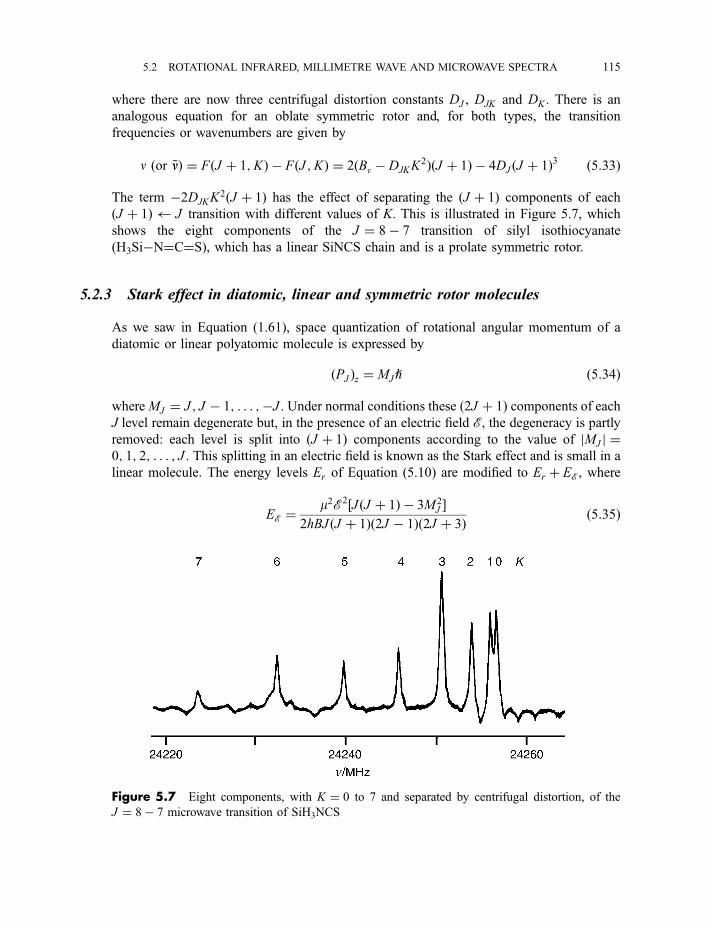
where there are now three centrifugal distortion constants DJ , DJK and DK . There is an
analogous equation for an oblate symmetric rotor and, for both types, the transition
frequencies or wavenumbers are given by
n ðor ~nnÞ ¼ FðJ þ 1;KÞ � FðJ ;KÞ ¼ 2ðBv � DJKK2ÞðJ þ 1Þ � 4DJ ðJ þ 1Þ3 ð5:33Þ
The term �2DJKK2ðJ þ 1Þ has the effect of separating the ðJ þ 1Þ components of each
ðJ þ 1Þ J transition with different values of K. This is illustrated in Figure 5.7, which
shows the eight components of the J ¼ 8� 7 transition of silyl isothiocyanate
(H3Si�N¼C¼S), which has a linear SiNCS chain and is a prolate symmetric rotor.
5.2.3 Stark effect in diatomic, linear and symmetric rotor molecules
As we saw in Equation (1.61), space quantization of rotational angular momentum of a
diatomic or linear polyatomic molecule is expressed by
ðPJ Þz ¼ MJh ð5:34Þ
whereMJ ¼ J ; J � 1; . . . ;�J . Under normal conditions these ð2J þ 1Þ components of each
J level remain degenerate but, in the presence of an electric field e, the degeneracy is partly
removed: each level is split into ðJ þ 1Þ components according to the value of jMJ j ¼0; 1; 2; . . . ; J . This splitting in an electric field is known as the Stark effect and is small in a
linear molecule. The energy levels Er of Equation (5.10) are modified to Er þ Ee, where
Ee ¼m2e2½J ðJ þ 1Þ � 3M 2
J �2hBJ ðJ þ 1Þð2J � 1Þð2J þ 3Þ ð5:35Þ
Figure 5.7 Eight components, with K ¼ 0 to 7 and separated by centrifugal distortion, of the
J ¼ 8� 7 microwave transition of SiH3NCS
5.2 ROTATIONAL INFRARED, MILLIMETRE WAVE AND MICROWAVE SPECTRA 115
In this rather formidable equation there are two points to notice:
1. It involves M2J , and therefore the energy is independent of the sign of MJ .
2. It involves the molecular dipole moment.
Because of point 2, rotational microwave and millimetre wave spectroscopy are powerful
techniques for determining dipole moments. However, the direction of the dipole moment
cannot be determined. In the case of O¼C¼S, for which m ¼ 0:715 21�0:000 20 D ½ð2:3857� 0:0007Þ � 10�30 C m�, a simple electronegativity argument leads
to the correct conclusion – that the oxygen end of the molecule is the negative end of the
dipole. However, in CO, the value of 0:112 D ð3:74� 10�31 C mÞ is so small that only
accurate electronic structure calculations can be relied upon to conclude correctly that the
carbon end is the negative one.
For a symmetric rotor the modification Ee to the rotational energy levels in an electric
field e is larger than in a linear molecule and is given, approximately, by
Ee ’�meKMJ
J ðJ þ 1Þ ð5:36Þ
Using the Stark effect, the dipole moment of, for example, CH3F has been found to be
1.857� 0.001 D [(6.194� 0.004)6 10730 C m].
5.2.4 Asymmetric rotor molecules
Although these molecules form much the largest group we shall take up the smallest space
in considering their rotational spectra. The reason for this is that there are no closed
formulae for their rotational term values. Instead, these term values can be determined
accurately only by a matrix diagonalization for each value of J, which remains a good
quantum number. The selection rule DJ ¼ 0, � 1 applies and the molecule must have a
permanent dipole moment.
At a simple level, the rotational transitions of near-symmetric rotors (see Equations 5.8
and 5.9) are easier to understand. For a prolate or oblate near-symmetric rotor the rotational
term values are given, approximately, by
FðJ ;KÞ ’ �BBJ ðJ þ 1Þ þ ðA� �BBÞK2 ð5:37Þ
and
FðJ ;KÞ ’ �BBJ ðJ þ 1Þ þ ðC � �BBÞK2 ð5:38Þ
respectively, where �BB is equal to 12ðBþ CÞ for a prolate rotor and 1
2ðAþ BÞ for an oblate
rotor. Centrifugal distortion has been neglected. Because the molecules concerned are only
approximately symmetric rotors K is not strictly a good quantum number (i.e. does not take
integral values).
116 5 ROTATIONAL SPECTROSCOPY
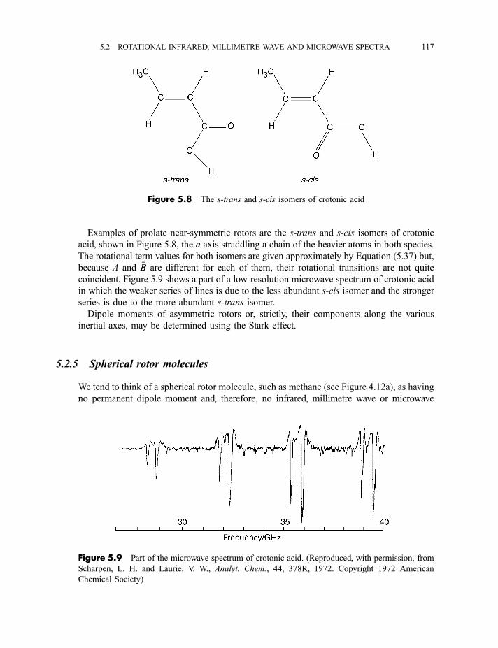
Examples of prolate near-symmetric rotors are the s-trans and s-cis isomers of crotonic
acid, shown in Figure 5.8, the a axis straddling a chain of the heavier atoms in both species.
The rotational term values for both isomers are given approximately by Equation (5.37) but,
because A and �BB are different for each of them, their rotational transitions are not quite
coincident. Figure 5.9 shows a part of a low-resolution microwave spectrum of crotonic acid
in which the weaker series of lines is due to the less abundant s-cis isomer and the stronger
series is due to the more abundant s-trans isomer.
Dipole moments of asymmetric rotors or, strictly, their components along the various
inertial axes, may be determined using the Stark effect.
5.2.5 Spherical rotor molecules
We tend to think of a spherical rotor molecule, such as methane (see Figure 4.12a), as having
no permanent dipole moment and, therefore, no infrared, millimetre wave or microwave
Figure 5.8 The s-trans and s-cis isomers of crotonic acid
Figure 5.9 Part of the microwave spectrum of crotonic acid. (Reproduced, with permission, from
Scharpen, L. H. and Laurie, V. W., Analyt. Chem., 44, 378R, 1972. Copyright 1972 American
Chemical Society)
5.2 ROTATIONAL INFRARED, MILLIMETRE WAVE AND MICROWAVE SPECTRA 117
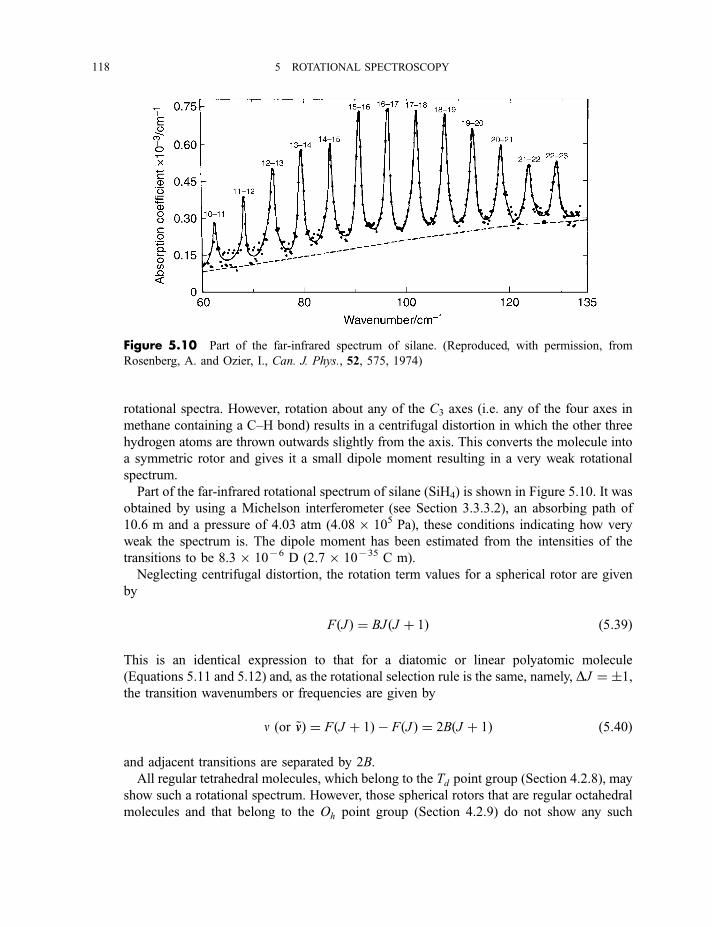
rotational spectra. However, rotation about any of the C3 axes (i.e. any of the four axes in
methane containing a C–H bond) results in a centrifugal distortion in which the other three
hydrogen atoms are thrown outwards slightly from the axis. This converts the molecule into
a symmetric rotor and gives it a small dipole moment resulting in a very weak rotational
spectrum.
Part of the far-infrared rotational spectrum of silane (SiH4) is shown in Figure 5.10. It was
obtained by using a Michelson interferometer (see Section 3.3.3.2), an absorbing path of
10.6 m and a pressure of 4.03 atm (4.086 105 Pa), these conditions indicating how very
weak the spectrum is. The dipole moment has been estimated from the intensities of the
transitions to be 8.36 1076 D (2.76 10735 C m).
Neglecting centrifugal distortion, the rotation term values for a spherical rotor are given
by
FðJ Þ ¼ BJ ðJ þ 1Þ ð5:39Þ
This is an identical expression to that for a diatomic or linear polyatomic molecule
(Equations 5.11 and 5.12) and, as the rotational selection rule is the same, namely, DJ ¼ �1,the transition wavenumbers or frequencies are given by
n ðor ~nnÞ ¼ FðJ þ 1Þ � FðJ Þ ¼ 2BðJ þ 1Þ ð5:40Þ
and adjacent transitions are separated by 2B.
All regular tetrahedral molecules, which belong to the Td point group (Section 4.2.8), may
show such a rotational spectrum. However, those spherical rotors that are regular octahedral
molecules and that belong to the Oh point group (Section 4.2.9) do not show any such
Figure 5.10 Part of the far-infrared spectrum of silane. (Reproduced, with permission, from
Rosenberg, A. and Ozier, I., Can. J. Phys., 52, 575, 1974)
118 5 ROTATIONAL SPECTROSCOPY
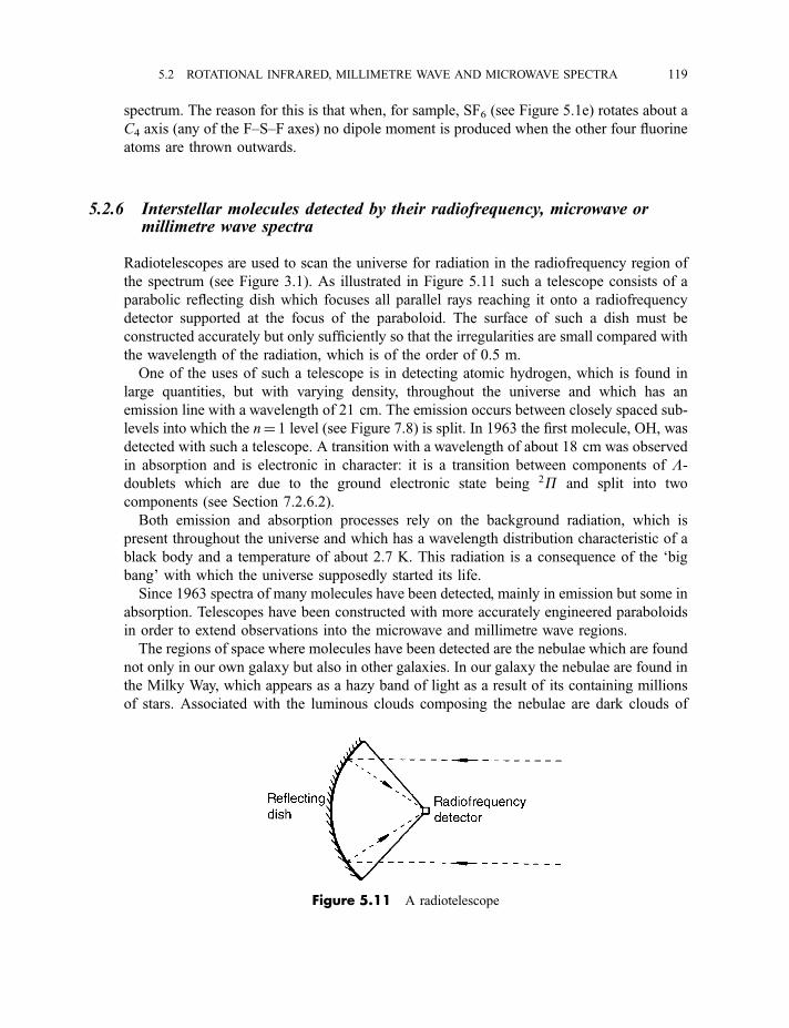
spectrum. The reason for this is that when, for sample, SF6 (see Figure 5.1e) rotates about a
C4 axis (any of the F–S–F axes) no dipole moment is produced when the other four fluorine
atoms are thrown outwards.
5.2.6 Interstellar molecules detected by their radiofrequency, microwave ormillimetre wave spectra
Radiotelescopes are used to scan the universe for radiation in the radiofrequency region of
the spectrum (see Figure 3.1). As illustrated in Figure 5.11 such a telescope consists of a
parabolic reflecting dish which focuses all parallel rays reaching it onto a radiofrequency
detector supported at the focus of the paraboloid. The surface of such a dish must be
constructed accurately but only sufficiently so that the irregularities are small compared with
the wavelength of the radiation, which is of the order of 0.5 m.
One of the uses of such a telescope is in detecting atomic hydrogen, which is found in
large quantities, but with varying density, throughout the universe and which has an
emission line with a wavelength of 21 cm. The emission occurs between closely spaced sub-
levels into which the n¼ 1 level (see Figure 7.8) is split. In 1963 the first molecule, OH, was
detected with such a telescope. A transition with a wavelength of about 18 cm was observed
in absorption and is electronic in character: it is a transition between components of L-doublets which are due to the ground electronic state being 2P and split into two
components (see Section 7.2.6.2).
Both emission and absorption processes rely on the background radiation, which is
present throughout the universe and which has a wavelength distribution characteristic of a
black body and a temperature of about 2.7 K. This radiation is a consequence of the ‘big
bang’ with which the universe supposedly started its life.
Since 1963 spectra of many molecules have been detected, mainly in emission but some in
absorption. Telescopes have been constructed with more accurately engineered paraboloids
in order to extend observations into the microwave and millimetre wave regions.
The regions of space where molecules have been detected are the nebulae which are found
not only in our own galaxy but also in other galaxies. In our galaxy the nebulae are found in
the Milky Way, which appears as a hazy band of light as a result of its containing millions
of stars. Associated with the luminous clouds composing the nebulae are dark clouds of
Figure 5.11 A radiotelescope
5.2 ROTATIONAL INFRARED, MILLIMETRE WAVE AND MICROWAVE SPECTRA 119
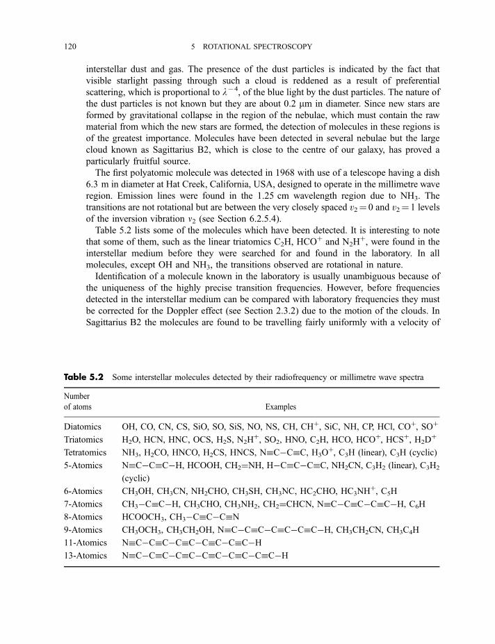
interstellar dust and gas. The presence of the dust particles is indicated by the fact that
visible starlight passing through such a cloud is reddened as a result of preferential
scattering, which is proportional to l74, of the blue light by the dust particles. The nature of
the dust particles is not known but they are about 0.2 mm in diameter. Since new stars are
formed by gravitational collapse in the region of the nebulae, which must contain the raw
material from which the new stars are formed, the detection of molecules in these regions is
of the greatest importance. Molecules have been detected in several nebulae but the large
cloud known as Sagittarius B2, which is close to the centre of our galaxy, has proved a
particularly fruitful source.
The first polyatomic molecule was detected in 1968 with use of a telescope having a dish
6.3 m in diameter at Hat Creek, California, USA, designed to operate in the millimetre wave
region. Emission lines were found in the 1.25 cm wavelength region due to NH3. The
transitions are not rotational but are between the very closely spaced v2¼ 0 and v2¼ 1 levels
of the inversion vibration n2 (see Section 6.2.5.4).
Table 5.2 lists some of the molecules which have been detected. It is interesting to note
that some of them, such as the linear triatomics C2H, HCOþ and N2H
þ, were found in the
interstellar medium before they were searched for and found in the laboratory. In all
molecules, except OH and NH3, the transitions observed are rotational in nature.
Identification of a molecule known in the laboratory is usually unambiguous because of
the uniqueness of the highly precise transition frequencies. However, before frequencies
detected in the interstellar medium can be compared with laboratory frequencies they must
be corrected for the Doppler effect (see Section 2.3.2) due to the motion of the clouds. In
Sagittarius B2 the molecules are found to be travelling fairly uniformly with a velocity of
Table 5.2 Some interstellar molecules detected by their radiofrequency or millimetre wave spectra
Number
of atoms Examples
Diatomics OH, CO, CN, CS, SiO, SO, SiS, NO, NS, CH, CHþ, SiC, NH, CP, HCl, COþ, SOþ
Triatomics H2O, HCN, HNC, OCS, H2S, N2Hþ, SO2, HNO, C2H, HCO, HCO
þ, HCSþ, H2Dþ
Tetratomics NH3, H2CO, HNCO, H2CS, HNCS, NC�CC, H3Oþ, C3H (linear), C3H (cyclic)
5-Atomics NC�CC�H, HCOOH, CH2¼NH, H�CC�CC, NH2CN, C3H2 (linear), C3H2
(cyclic)
6-Atomics CH3OH, CH3CN, NH2CHO, CH3SH, CH3NC, HC2CHO, HC3NHþ, C5H
7-Atomics CH3�CC�H, CH3CHO, CH3NH2, CH2¼CHCN, NC�CC�CC�H, C6H
8-Atomics HCOOCH3, CH3�CC�CN9-Atomics CH3OCH3, CH3CH2OH, NC�CC�CC�CC�H, CH3CH2CN, CH3C4H
11-Atomics NC�CC�CC�CC�CC�H13-Atomics NC�CC�CC�CC�CC�CC�H
120 5 ROTATIONAL SPECTROSCOPY
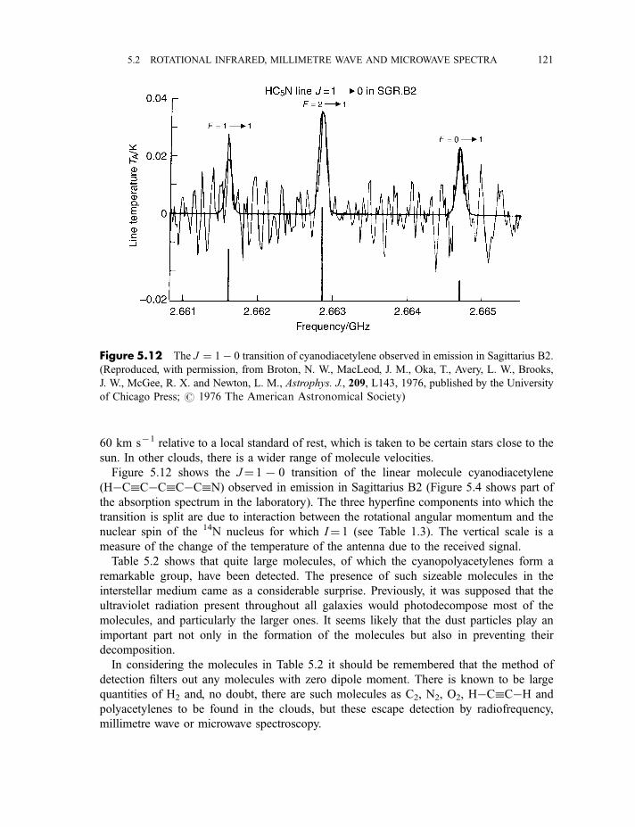
60 km s71 relative to a local standard of rest, which is taken to be certain stars close to the
sun. In other clouds, there is a wider range of molecule velocities.
Figure 5.12 shows the J¼ 17 0 transition of the linear molecule cyanodiacetylene
(H�CC�CC�CN) observed in emission in Sagittarius B2 (Figure 5.4 shows part of
the absorption spectrum in the laboratory). The three hyperfine components into which the
transition is split are due to interaction between the rotational angular momentum and the
nuclear spin of the 14N nucleus for which I¼ 1 (see Table 1.3). The vertical scale is a
measure of the change of the temperature of the antenna due to the received signal.
Table 5.2 shows that quite large molecules, of which the cyanopolyacetylenes form a
remarkable group, have been detected. The presence of such sizeable molecules in the
interstellar medium came as a considerable surprise. Previously, it was supposed that the
ultraviolet radiation present throughout all galaxies would photodecompose most of the
molecules, and particularly the larger ones. It seems likely that the dust particles play an
important part not only in the formation of the molecules but also in preventing their
decomposition.
In considering the molecules in Table 5.2 it should be remembered that the method of
detection filters out any molecules with zero dipole moment. There is known to be large
quantities of H2 and, no doubt, there are such molecules as C2, N2, O2, H�CC�H and
polyacetylenes to be found in the clouds, but these escape detection by radiofrequency,
millimetre wave or microwave spectroscopy.
Figure 5.12 The J ¼ 1� 0 transition of cyanodiacetylene observed in emission in Sagittarius B2.
(Reproduced, with permission, from Broton, N. W., MacLeod, J. M., Oka, T., Avery, L. W., Brooks,
J. W., McGee, R. X. and Newton, L. M., Astrophys. J., 209, L143, 1976, published by the University
of Chicago Press; # 1976 The American Astronomical Society)
5.2 ROTATIONAL INFRARED, MILLIMETRE WAVE AND MICROWAVE SPECTRA 121
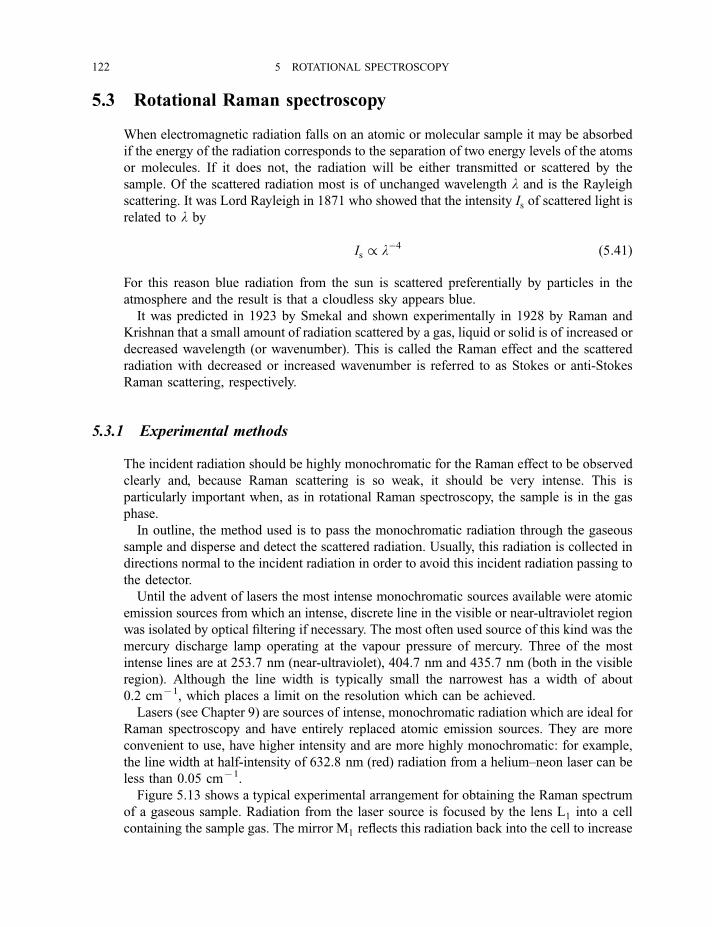
5.3 Rotational Raman spectroscopy
When electromagnetic radiation falls on an atomic or molecular sample it may be absorbed
if the energy of the radiation corresponds to the separation of two energy levels of the atoms
or molecules. If it does not, the radiation will be either transmitted or scattered by the
sample. Of the scattered radiation most is of unchanged wavelength l and is the Rayleigh
scattering. It was Lord Rayleigh in 1871 who showed that the intensity Is of scattered light is
related to l by
Is / l�4 ð5:41Þ
For this reason blue radiation from the sun is scattered preferentially by particles in the
atmosphere and the result is that a cloudless sky appears blue.
It was predicted in 1923 by Smekal and shown experimentally in 1928 by Raman and
Krishnan that a small amount of radiation scattered by a gas, liquid or solid is of increased or
decreased wavelength (or wavenumber). This is called the Raman effect and the scattered
radiation with decreased or increased wavenumber is referred to as Stokes or anti-Stokes
Raman scattering, respectively.
5.3.1 Experimental methods
The incident radiation should be highly monochromatic for the Raman effect to be observed
clearly and, because Raman scattering is so weak, it should be very intense. This is
particularly important when, as in rotational Raman spectroscopy, the sample is in the gas
phase.
In outline, the method used is to pass the monochromatic radiation through the gaseous
sample and disperse and detect the scattered radiation. Usually, this radiation is collected in
directions normal to the incident radiation in order to avoid this incident radiation passing to
the detector.
Until the advent of lasers the most intense monochromatic sources available were atomic
emission sources from which an intense, discrete line in the visible or near-ultraviolet region
was isolated by optical filtering if necessary. The most often used source of this kind was the
mercury discharge lamp operating at the vapour pressure of mercury. Three of the most
intense lines are at 253.7 nm (near-ultraviolet), 404.7 nm and 435.7 nm (both in the visible
region). Although the line width is typically small the narrowest has a width of about
0.2 cm71, which places a limit on the resolution which can be achieved.
Lasers (see Chapter 9) are sources of intense, monochromatic radiation which are ideal for
Raman spectroscopy and have entirely replaced atomic emission sources. They are more
convenient to use, have higher intensity and are more highly monochromatic: for example,
the line width at half-intensity of 632.8 nm (red) radiation from a helium–neon laser can be
less than 0.05 cm71.
Figure 5.13 shows a typical experimental arrangement for obtaining the Raman spectrum
of a gaseous sample. Radiation from the laser source is focused by the lens L1 into a cell
containing the sample gas. The mirror M1 reflects this radiation back into the cell to increase
122 5 ROTATIONAL SPECTROSCOPY
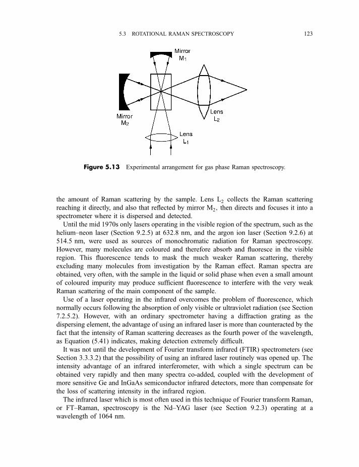
the amount of Raman scattering by the sample. Lens L2 collects the Raman scattering
reaching it directly, and also that reflected by mirror M2; then directs and focuses it into a
spectrometer where it is dispersed and detected.
Until the mid 1970s only lasers operating in the visible region of the spectrum, such as the
helium–neon laser (Section 9.2.5) at 632.8 nm, and the argon ion laser (Section 9.2.6) at
514.5 nm, were used as sources of monochromatic radiation for Raman spectroscopy.
However, many molecules are coloured and therefore absorb and fluoresce in the visible
region. This fluorescence tends to mask the much weaker Raman scattering, thereby
excluding many molecules from investigation by the Raman effect. Raman spectra are
obtained, very often, with the sample in the liquid or solid phase when even a small amount
of coloured impurity may produce sufficient fluorescence to interfere with the very weak
Raman scattering of the main component of the sample.
Use of a laser operating in the infrared overcomes the problem of fluorescence, which
normally occurs following the absorption of only visible or ultraviolet radiation (see Section
7.2.5.2). However, with an ordinary spectrometer having a diffraction grating as the
dispersing element, the advantage of using an infrared laser is more than counteracted by the
fact that the intensity of Raman scattering decreases as the fourth power of the wavelength,
as Equation (5.41) indicates, making detection extremely difficult.
It was not until the development of Fourier transform infrared (FTIR) spectrometers (see
Section 3.3.3.2) that the possibility of using an infrared laser routinely was opened up. The
intensity advantage of an infrared interferometer, with which a single spectrum can be
obtained very rapidly and then many spectra co-added, coupled with the development of
more sensitive Ge and InGaAs semiconductor infrared detectors, more than compensate for
the loss of scattering intensity in the infrared region.
The infrared laser which is most often used in this technique of Fourier transform Raman,
or FT–Raman, spectroscopy is the Nd–YAG laser (see Section 9.2.3) operating at a
wavelength of 1064 nm.
Figure 5.13 Experimental arrangement for gas phase Raman spectroscopy.
5.3 ROTATIONAL RAMAN SPECTROSCOPY 123
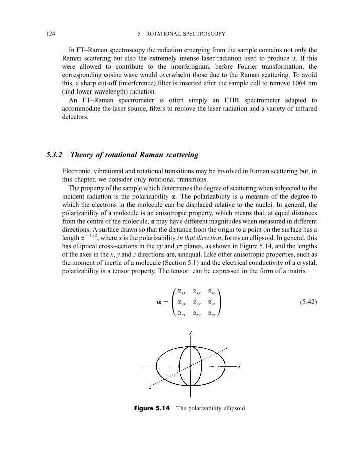
In FT–Raman spectroscopy the radiation emerging from the sample contains not only the
Raman scattering but also the extremely intense laser radiation used to produce it. If this
were allowed to contribute to the interferogram, before Fourier transformation, the
corresponding cosine wave would overwhelm those due to the Raman scattering. To avoid
this, a sharp cut-off (interference) filter is inserted after the sample cell to remove 1064 nm
(and lower wavelength) radiation.
An FT–Raman spectrometer is often simply an FTIR spectrometer adapted to
accommodate the laser source, filters to remove the laser radiation and a variety of infrared
detectors.
5.3.2 Theory of rotational Raman scattering
Electronic, vibrational and rotational transitions may be involved in Raman scattering but, in
this chapter, we consider only rotational transitions.
The property of the sample which determines the degree of scattering when subjected to the
incident radiation is the polarizability aa. The polarizability is a measure of the degree to
which the electrons in the molecule can be displaced relative to the nuclei. In general, the
polarizability of a molecule is an anisotropic property, which means that, at equal distances
from the centre of the molecule, aamay have different magnitudes when measured in different
directions. A surface drawn so that the distance from the origin to a point on the surface has a
length a71=2, where a is the polarizability in that direction, forms an ellipsoid. In general, this
has elliptical cross-sections in the xy and yz planes, as shown in Figure 5.14, and the lengths
of the axes in the x, y and z directions are, unequal. Like other anisotropic properties, such as
the moment of inertia of a molecule (Section 5.1) and the electrical conductivity of a crystal,
polarizability is a tensor property. The tensor can be expressed in the form of a matrix:
a ¼axx axy axzayx ayy ayzazx azy azz
0B@
1CA ð5:42Þ
Figure 5.14 The polarizability ellipsoid
124 5 ROTATIONAL SPECTROSCOPY
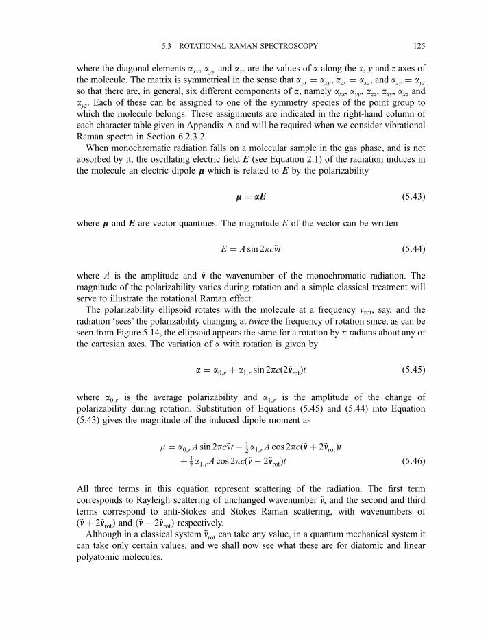
where the diagonal elements axx, ayy and azz are the values of a along the x, y and z axes of
the molecule. The matrix is symmetrical in the sense that ayx ¼ axy, azx ¼ axz, and azy ¼ ayzso that there are, in general, six different components of a, namely axx, ayy, azz, axy, axz andayz. Each of these can be assigned to one of the symmetry species of the point group to
which the molecule belongs. These assignments are indicated in the right-hand column of
each character table given in Appendix A and will be required when we consider vibrational
Raman spectra in Section 6.2.3.2.
When monochromatic radiation falls on a molecular sample in the gas phase, and is not
absorbed by it, the oscillating electric field E (see Equation 2.1) of the radiation induces in
the molecule an electric dipole mm which is related to E by the polarizability
mm ¼ aaE ð5:43Þ
where mm and E are vector quantities. The magnitude E of the vector can be written
E ¼ A sin 2pc~nnt ð5:44Þ
where A is the amplitude and ~nn the wavenumber of the monochromatic radiation. The
magnitude of the polarizability varies during rotation and a simple classical treatment will
serve to illustrate the rotational Raman effect.
The polarizability ellipsoid rotates with the molecule at a frequency nrot, say, and the
radiation ‘sees’ the polarizability changing at twice the frequency of rotation since, as can be
seen from Figure 5.14, the ellipsoid appears the same for a rotation by p radians about any of
the cartesian axes. The variation of a with rotation is given by
a ¼ a0;r þ a1;r sin 2pcð2~nnrotÞt ð5:45Þ
where a0;r is the average polarizability and a1;r is the amplitude of the change of
polarizability during rotation. Substitution of Equations (5.45) and (5.44) into Equation
(5.43) gives the magnitude of the induced dipole moment as
m ¼ a0;r A sin 2pc~nnt � 12a1;r A cos 2pcð~nnþ 2~nnrotÞt
þ 12a1;r A cos 2pcð~nn� 2~nnrotÞt ð5:46Þ
All three terms in this equation represent scattering of the radiation. The first term
corresponds to Rayleigh scattering of unchanged wavenumber ~nn, and the second and third
terms correspond to anti-Stokes and Stokes Raman scattering, with wavenumbers of
ð~nnþ 2~nnrotÞ and ð~nn� 2~nnrotÞ respectively.Although in a classical system ~nnrot can take any value, in a quantum mechanical system it
can take only certain values, and we shall now see what these are for diatomic and linear
polyatomic molecules.
5.3 ROTATIONAL RAMAN SPECTROSCOPY 125
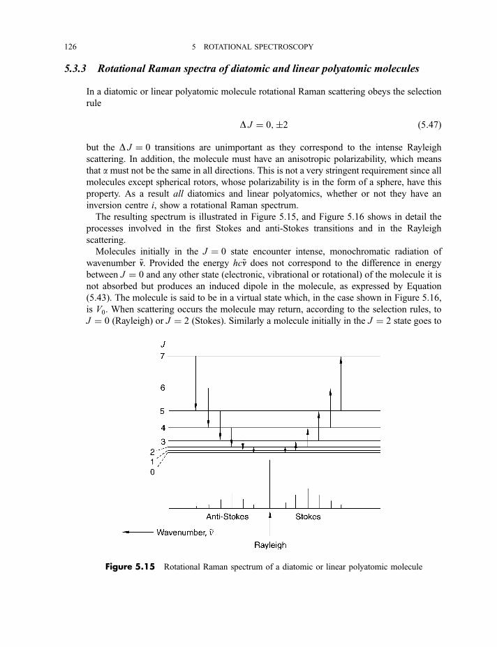
5.3.3 Rotational Raman spectra of diatomic and linear polyatomic molecules
In a diatomic or linear polyatomic molecule rotational Raman scattering obeys the selection
rule
D J ¼ 0;�2 ð5:47Þ
but the D J ¼ 0 transitions are unimportant as they correspond to the intense Rayleigh
scattering. In addition, the molecule must have an anisotropic polarizability, which means
that a must not be the same in all directions. This is not a very stringent requirement since all
molecules except spherical rotors, whose polarizability is in the form of a sphere, have this
property. As a result all diatomics and linear polyatomics, whether or not they have an
inversion centre i, show a rotational Raman spectrum.
The resulting spectrum is illustrated in Figure 5.15, and Figure 5.16 shows in detail the
processes involved in the first Stokes and anti-Stokes transitions and in the Rayleigh
scattering.
Molecules initially in the J ¼ 0 state encounter intense, monochromatic radiation of
wavenumber ~nn. Provided the energy hc~nn does not correspond to the difference in energy
between J ¼ 0 and any other state (electronic, vibrational or rotational) of the molecule it is
not absorbed but produces an induced dipole in the molecule, as expressed by Equation
(5.43). The molecule is said to be in a virtual state which, in the case shown in Figure 5.16,
is V0. When scattering occurs the molecule may return, according to the selection rules, to
J ¼ 0 (Rayleigh) or J ¼ 2 (Stokes). Similarly a molecule initially in the J ¼ 2 state goes to
Figure 5.15 Rotational Raman spectrum of a diatomic or linear polyatomic molecule
126 5 ROTATIONAL SPECTROSCOPY
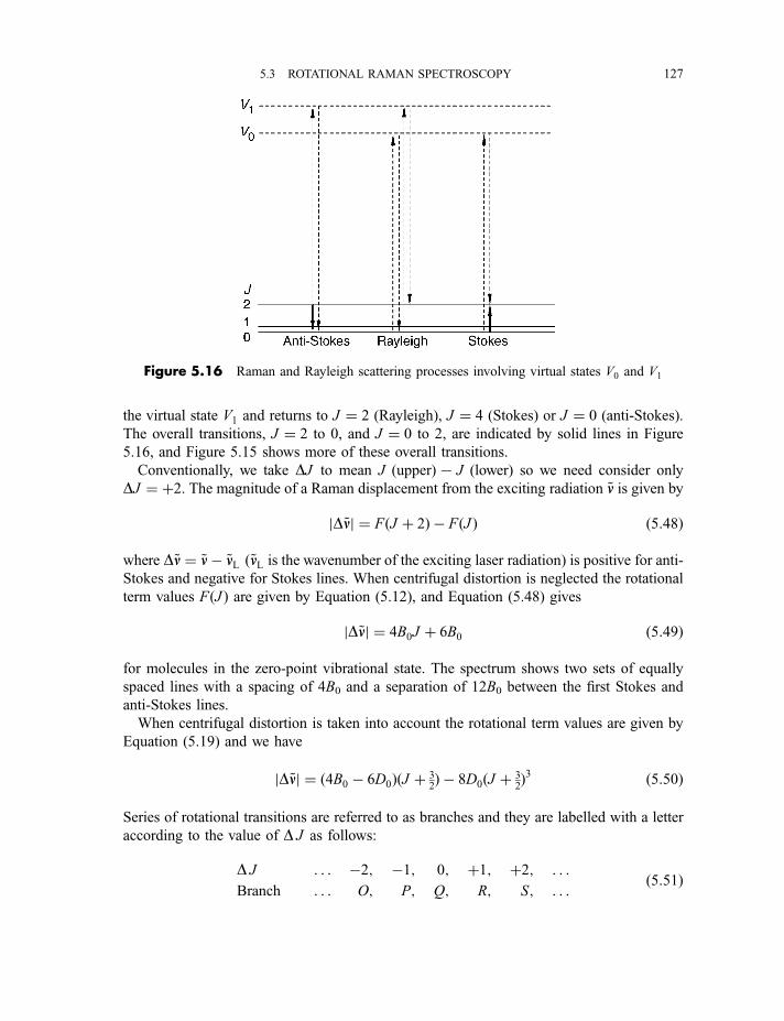
the virtual state V1 and returns to J ¼ 2 (Rayleigh), J ¼ 4 (Stokes) or J ¼ 0 (anti-Stokes).
The overall transitions, J ¼ 2 to 0, and J ¼ 0 to 2, are indicated by solid lines in Figure
5.16, and Figure 5.15 shows more of these overall transitions.
Conventionally, we take DJ to mean J (upper)7 J (lower) so we need consider only
DJ ¼ þ2. The magnitude of a Raman displacement from the exciting radiation ~nn is given by
jD~nnj ¼ FðJ þ 2Þ � FðJ Þ ð5:48Þ
where D~nn ¼ ~nn� ~nnL ð~nnL is the wavenumber of the exciting laser radiation) is positive for anti-
Stokes and negative for Stokes lines. When centrifugal distortion is neglected the rotational
term values FðJ Þ are given by Equation (5.12), and Equation (5.48) gives
jD~nnj ¼ 4B0J þ 6B0 ð5:49Þ
for molecules in the zero-point vibrational state. The spectrum shows two sets of equally
spaced lines with a spacing of 4B0 and a separation of 12B0 between the first Stokes and
anti-Stokes lines.
When centrifugal distortion is taken into account the rotational term values are given by
Equation (5.19) and we have
jD~nnj ¼ ð4B0 � 6D0ÞðJ þ 32Þ � 8D0ðJ þ 3
2Þ3 ð5:50Þ
Series of rotational transitions are referred to as branches and they are labelled with a letter
according to the value of D J as follows:
D J
Branch
. . .
. . .
�2;O;
�1;P;
0;
Q;
þ1;R;
þ2;S;
. . .
. . .ð5:51Þ
Figure 5.16 Raman and Rayleigh scattering processes involving virtual states V0 and V1
5.3 ROTATIONAL RAMAN SPECTROSCOPY 127
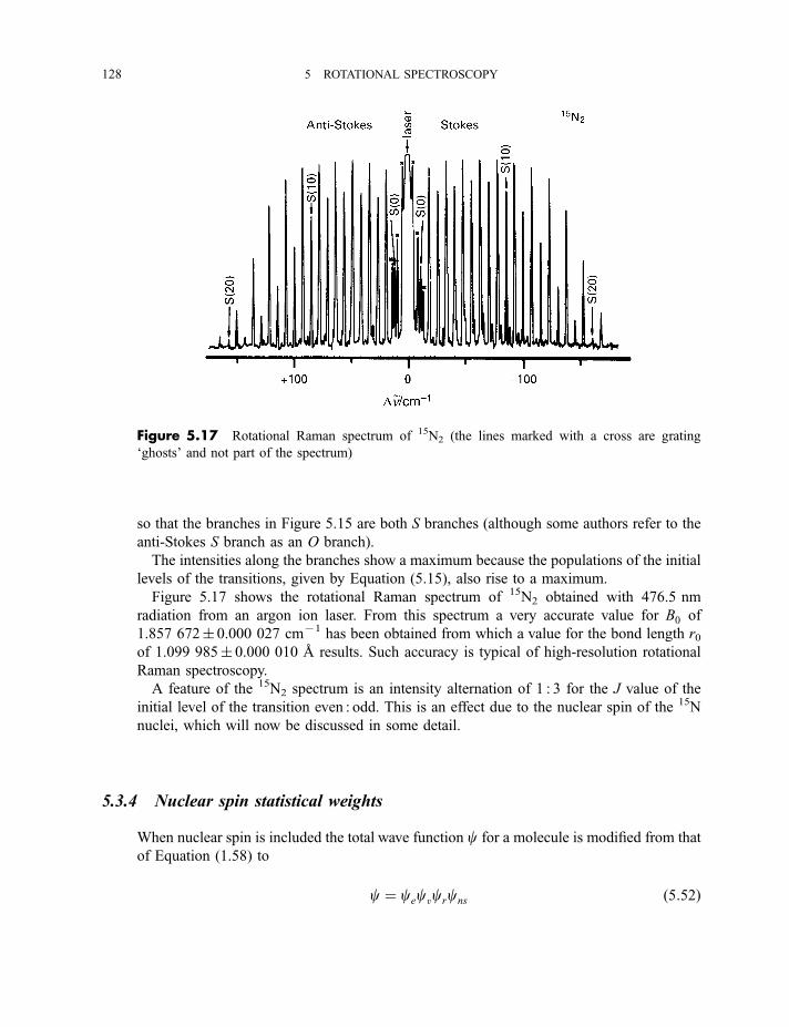
so that the branches in Figure 5.15 are both S branches (although some authors refer to the
anti-Stokes S branch as an O branch).
The intensities along the branches show a maximum because the populations of the initial
levels of the transitions, given by Equation (5.15), also rise to a maximum.
Figure 5.17 shows the rotational Raman spectrum of 15N2 obtained with 476.5 nm
radiation from an argon ion laser. From this spectrum a very accurate value for B0 of
1.857 672� 0.000 027 cm71 has been obtained from which a value for the bond length r0of 1.099 985� 0.000 010 A results. Such accuracy is typical of high-resolution rotational
Raman spectroscopy.
A feature of the 15N2 spectrum is an intensity alternation of 1 : 3 for the J value of the
initial level of the transition even : odd. This is an effect due to the nuclear spin of the 15N
nuclei, which will now be discussed in some detail.
5.3.4 Nuclear spin statistical weights
When nuclear spin is included the total wave function c for a molecule is modified from that
of Equation (1.58) to
c ¼ cecvcrcns ð5:52Þ
Figure 5.17 Rotational Raman spectrum of 15N2 (the lines marked with a cross are grating
‘ghosts’ and not part of the spectrum)
128 5 ROTATIONAL SPECTROSCOPY
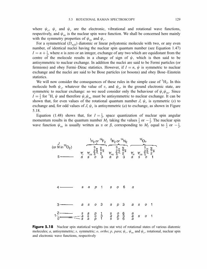
where ce, cv and cr are the electronic, vibrational and rotational wave functions,
respectively, and cns is the nuclear spin wave function. We shall be concerned here mainly
with the symmetry properties of cns and cr.
For a symmetrical (D1h) diatomic or linear polyatomic molecule with two, or any even
number, of identical nuclei having the nuclear spin quantum number (see Equation 1.47)
I ¼ nþ 12, where n is zero or an integer, exchange of any two which are equidistant from the
centre of the molecule results in a change of sign of c; which is then said to be
antisymmetric to nuclear exchange. In addition the nuclei are said to be Fermi particles (or
fermions) and obey Fermi–Dirac statistics. However, if I ¼ n, c is symmetric to nuclear
exchange and the nuclei are said to be Bose particles (or bosons) and obey Bose–Einstein
statistics.
We will now consider the consequences of these rules in the simple case of 1H2. In this
molecule both cv, whatever the value of v, and ce, in the ground electronic state, are
symmetric to nuclear exchange: so we need consider only the behaviour of crcns. Since
I ¼ 12for 1H, c and therefore crcns must be antisymmetric to nuclear exchange. It can be
shown that, for even values of the rotational quantum number J, cr is symmetric (s) to
exchange and, for odd values of J, cr is antisymmetric (a) to exchange, as shown in Figure
5.18.
Equation (1.48) shows that, for I ¼ 12, space quantization of nuclear spin angular
momentum results in the quantum number MI taking the values 12or � 1
2. The nuclear spin
wave function cns is usually written as a or b, corresponding to MI equal to 12or � 1
2,
Figure 5.18 Nuclear spin statistical weights (ns stat wts) of rotational states of various diatomic
molecules; a, antisymmetric; s; symmetric; o; ortho; p; para; cr; cns and ce; rotational, nuclear spinand electronic wave functions, respectively
5.3 ROTATIONAL RAMAN SPECTROSCOPY 129
respectively, and both 1H nuclei, labelled 1 and 2, can have either a or b spin wave functions.
There are therefore four possible forms of cns for the molecule as a whole:
cns ¼ að1Það2Þ; bð1Þbð2Þ; að1Þbð2Þ; or bð1Það2Þ ð5:53Þ
Although the að1Það2Þ and bð1Þbð2Þ wave functions are clearly symmetric to interchange of
the 1 and 2 labels, the other two functions are neither symmetric nor antisymmetric. For this
reason it is necessary to use instead the linear combinations 2�1=2½að1Þbð2Þ þ bð1Það2Þ� and2�1=2½að1Þbð2Þ � bð1Það2Þ�, where 271=2 is a normalization constant. Then three of the four
nuclear spin wave functions are seen to be symmetric (s) to nuclear exchange and one is
antisymmetric (a):
ðsÞ cns ¼að1Það2Þ2�1=2½að1Þbð2Þ þ bð1Það2Þ�bð1Þbð2Þ
8><>: ð5:54Þ
ðaÞ cns ¼ 2�1=2½að1Þbð2Þ � bð1Það2Þ� ð5:55Þ
In general, for a homonuclear diatomic molecule there are (2Iþ 1)(Iþ 1) symmetric and
(2Iþ 1)I antisymmetric nuclear spin wave functions; therefore
Number of ðsÞ functionsNumber of ðaÞ functions ¼
I þ 1
Ið5:56Þ
In order that crcns is always antisymmetric for 1H2 the antisymmetric cns are associated
with even J states and the symmetric cns with odd J states, as shown in Figure 5.18.
Interchange between states with cns symmetric and antisymmetric is forbidden so that 1H2
can be regarded as consisting of two distinct forms:
1. para-hydrogen with cns antisymmetric and with what is commonly referred to as
antiparallel nuclear spins;
2. ortho-hydrogen with cns symmetric and parallel nuclear spins.
As indicated in Figure 5.18, para-1H2 can exist in only even J states and ortho-1H2 in odd
J states. At temperatures at which there is appreciable population up to fairly high values of
J there is roughly three times as much ortho- as there is para-1H2. However, at very low
temperatures at which the population of all rotational levels other than J¼ 0 is small 1H2 is
mostly in the para form.
All other homonuclear diatomic molecules with I ¼ 12for each nucleus, such as 19F2, also
have ortho and para forms with odd and even J and nuclear spin statistical weights of 3 and
1, respectively, as shown in Figure 5.18.
If I ¼ 1 for each nucleus, as in 2H2 and14N2, the total wave function must be symmetric
to nuclear exchange. There are nine nuclear spin wave functions of which six are symmetric
and three antisymmetric to exchange. Figure 5.18 illustrates the fact that ortho-2H2 (or14N2)
130 5 ROTATIONAL SPECTROSCOPY
can have only even J and the para form only odd J, and that there is roughly twice as much
of the ortho form as there is of the para form at normal temperatures: at low temperatures
there is a larger excess of the ortho form.
The effect of low temperatures affecting the ortho : para ratio is more important for light
molecules, such as 1H2 and2H2, than for heavy ones, such as 19F2 and
14N2. The reason is
that the separation of the J¼ 0 and J¼ 1 levels is smaller for a heavier molecule and a lower
temperature is required before a significant deviation from the normal ortho : para ratio is
observed.
For the symmetrical linear polyatomic molecule acetylene
1H�12C12C�1H
the situation is very similar to that for 1H2 since I ¼ 0 for 12C. The main difference is that,
since the rotational energy levels are much more closely spaced, a much lower temperature is
necessary to produce acetylene predominantly in the para form.
For 16O, I is zero and there are no antisymmetric nuclear spin wave functions for 16O2.
Since each 16O nucleus is a boson the total wave function must be symmetric to nuclear
exchange. In the case of 16O2, with two electrons with unpaired spins in the ground state (see
Section 7.2.1.1), ce is antisymmetric, unlike the other molecules we have considered. Since
I ¼ 0 the nuclear spin wave function cns is equal to 1, which is symmetric to the exchange
of nuclei. Therefore, as Figure 5.18 shows, 16O2 has only levels with the rotational quantum
number having odd values and, in its rotational Raman spectrum, alternate lines with N 00
even are missing. (In molecules such as 16O2, which have a resultant electron spin angular
momentum due to unpaired electrons, the quantum number N, rather than J, distinguishes
the rotational levels.)
5.3.5 Rotational Raman spectra of symmetric and asymmetric rotormolecules
For a symmetric rotor molecule the selection rules for the rotational Raman spectrum are
D J ¼ 0;�1;�2; DK ¼ 0 ð5:57Þ
resulting in R and S branches for each value of K, in addition to the Rayleigh scattering.
For asymmetric rotors the selection rule in J is D J ¼ 0, � 1, � 2, but the fact that K is
not a good quantum number results in the additional selection rules being too complex for
discussion here.
5.4 Structure determination from rotational constants
Measurement and assignment of the rotational spectrum of a diatomic or other linear
molecule result in a value of the rotational constant. In general, this will be B0, which relates
5.4 STRUCTURE DETERMINATION FROM ROTATIONAL CONSTANTS 131
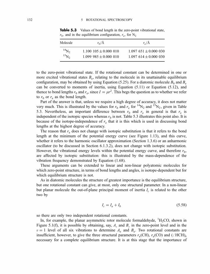
to the zero-point vibrational state. If the rotational constant can be determined in one or
more excited vibrational states Be, relating to the molecule in its unattainable equilibrium
configuration, may be obtained by using Equation (5.25). For a diatomic molecule B0 and Be
can be converted to moments of inertia, using Equation (5.11) or Equation (5.12), and
thence to bond lengths r0 and re, since I ¼ mr2. This begs the question as to whether we referto r0 or re as the bond length.
Part of the answer is that, unless we require a high degree of accuracy, it does not matter
very much. This is illustrated by the values for r0 and re for14N2 and
15N2, given in Table
5.3. Nevertheless, an important difference between r0 and re in general is that re is
independent of the isotopic species whereas r0 is not. Table 5.3 illustrates this point also. It is
because of the isotope-independence of re that it is this which is used in discussing bond
lengths at the highest degree of accuracy.
The reason that re does not change with isotopic substitution is that it refers to the bond
length at the minimum of the potential energy curve (see Figure 1.13), and this curve,
whether it refers to the harmonic oscillator approximation (Section 1.3.6) or an anharmonic
oscillator (to be discussed in Section 6.1.3.2), does not change with isotopic substitution.
However, the vibrational energy levels within the potential energy curve, and therefore r0,
are affected by isotopic substitution: this is illustrated by the mass-dependence of the
vibration frequency demonstrated by Equation (1.68).
These arguments can be extended to linear and non-linear polyatomic molecules for
which zero-point structure, in terms of bond lengths and angles, is isotope-dependent but for
which equilibrium structure is not.
As in diatomic molecules the structure of greatest importance is the equilibrium structure,
but one rotational constant can give, at most, only one structural parameter. In a non-linear
but planar molecule the out-of-plane principal moment of inertia Ic is related to the other
two by
Ic ¼ Ia þ Ib ð5:58Þ
so there are only two independent rotational constants.
In, for example, the planar asymmetric rotor molecule formaldehyde, 1H2CO, shown in
Figure 5.1(f), it is possible by obtaining, say, Av and Bv in the zero-point level and in the
v ¼ 1 level of all six vibrations to determine Ae and Be. Two rotational constants are
insufficient, however, to give the three structural parameters re(CH), re(CO) and (ffHCH)enecessary for a complete equilibrium structure. It is at this stage that the importance of
Table 5.3 Values of bond length in the zero-point vibrational state,
r0; and in the equilibrium configuration, re, for N2
Molecule r0=A re=A
14N2 1.100 105� 0.000 010 1.097 651� 0.000 03015N2 1.099 985� 0.000 010 1.097 614� 0.000 030
132 5 ROTATIONAL SPECTROSCOPY
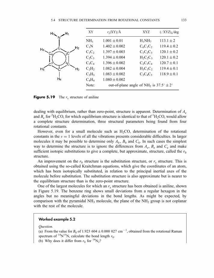
dealing with equilibrium, rather than zero-point, structure is apparent. Determination of Ae
and Be for2H2CO, for which equilibrium structure is identical to that of 1H2CO, would allow
a complete structure determination, three structural parameters being found from four
rotational constants.
However, even for a small molecule such as H2CO, determination of the rotational
constants in the v ¼ 1 levels of all the vibrations presents considerable difficulties. In larger
molecules it may be possible to determine only A0 , B0 and C0. In such cases the simplest
way to determine the structure is to ignore the differences from Ae, Be and Ce and make
sufficient isotopic substitutions to give a complete, but approximate, structure, called the r0structure.
An improvement on the r0 structure is the substitution structure, or rs structure. This is
obtained using the so-called Kraitchman equations, which give the coordinates of an atom,
which has been isotopically substituted, in relation to the principal inertial axes of the
molecule before substitution. The substitution structure is also approximate but is nearer to
the equilibrium structure than is the zero-point structure.
One of the largest molecules for which an rs structure has been obtained is aniline, shown
in Figure 5.19. The benzene ring shows small deviations from a regular hexagon in the
angles but no meaningful deviations in the bond lengths. As might be expected, by
comparison with the pyramidal NH3 molecule, the plane of the NH2 group is not coplanar
with the rest of the molecule.
Worked example 5.2
Question.
(a) From the value for B0 of 1.923 604� 0.000 027 cm71, obtained from the rotational Raman
spectrum of 14N15N, calculate the bond length r0.
(b) Why does it differ from r0 for 14N2?
Figure 5.19 The rs structure of aniline
XY rs(XY)=A XYZ (ffXYZ)s=deg
NH1 1.001� 0.01 H1NH7 113.1� 2
C1N 1.402� 0.002 C6C1C2 119.4� 0.2
C1C2 1.397� 0.003 C1C2C3 120.1� 0.2
C2C3 1.394� 0.004 H2C2C3 120.1� 0.2
C3C4 1.396� 0.002 C2C3C4 120.7� 0.1
C2H2 1.082� 0.004 H3C3C2 119.4� 0.1
C3H3 1.083� 0.002 C3C4C5 118.9� 0.1
C4H4 1.080� 0.002
Note: out-of-plane angle of NH2 is 37.5� � 2�
5.4 STRUCTURE DETERMINATION FROM ROTATIONAL CONSTANTS 133
(c) Would the values of re differ?
(d) Would there be an intensity alternation in the spectrum of 14N15N?
(e) Would 14N15N show a rotational infrared spectrum?
Answer.
(a) For 14N15N, reduced mass m is given by
m ¼ 14:003 07� 15:000 11
14:003 07þ 15:000 11g mol�1 � 10�3 kg g�1
6:022 142� 1023 mol�1
¼ 1:202 600� 10�26 kg
; r20 ¼h
8p2cmB0
¼ 6:626 069� 10�34 J s8p2 � 2:997 925� 1010 cm s�1 � 1:202 600� 10�26 kg� 1:923 604 cm�1
¼ 1:210 065� 10�20 m2
; r0 ¼ 1:100 03� 10�10 m
¼ 1:100 03 A�
Note that, since B0 is given, effectively, to six significant figures, the calculation has been done
to seven figures and rounded to six at the final stage.
(b) The calculated value of r0 differs from that of r0 ¼ 1:100 105 A for 14N2 (Table 5.3)
because the zero-point level is lower, within the same anharmonic potential (see Section 6.1.3),
for the heavier isotopic species. Therefore the mid-point of the zero-point level is at a smaller
value of the bond length. Note that this level of accuracy in the calculation is necessary to
illustrate this point.
(c) The values of re would not differ because they refer to the minimum of the isotope-
independent potential energy curve.
(d) There would be no intensity alternation in the spectrum of 14N15N because there is no
exchange of identical nuclei on rotation about an axis perpendicular to the bond.
(e) 14N15N would not show a rotational infrared spectum because 14N15N has no dipole
moment. (In fact, like all such isotopically unsymmetrical molecules, it has an extremely small
dipole moment, but too small for an infrared rotational spectrum to be detected.)
Exercises
5.1 Use Equation (5.16) to derive Equation (5.17). Compare values of Jmax and the
transition frequencies involving the values of Jmax for HCN (B ’ 44:316 GHz) and
NC�(CC)2�H ðB ’ 1:313 GHz).
134 5 ROTATIONAL SPECTROSCOPY
5.2 Rearrange Equation (5.20) into the form y ¼ mxþ c so that m involves D only. Plot y
against x using the data in Table 5.1 to obtain B and D, in hertz, for carbon monoxide
(use a computer or calculator that will work to nine-figure accuracy).
5.3 Make measurements of the transition wavenumbers in the rotational spectrum of silane
from Figure 5.10 and hence determine the Si�H bond length.
5.4 Assuming reasonable bond lengths, estimate the frequency of the J¼ 157 14 transition
in the linear molecule NC�(CC)6�H. In which region of the electromagnetic
spectrum does it lie?
5.5 Starting from an expression for rotational term values show that
jD~nnj ¼ ð4B0 � 6D0ÞðJ þ 32Þ � 8D0ðJ þ 3
2Þ3
for rotational Raman transitions of a diatomic or linear polyatomic molecule.
5.6 The first three Stokes lines in the rotational Raman spectrum of 16O2 are separated by
14.4 cm71, 25.8 cm71 and 37.4 cm71 from the exciting radiation. Using the rigid
rotor approximation obtain a value for r0.
Bibliography
Brown, J. M. and Carrington, A. (2003) Rotational Spectroscopy of Diatomic Molecules, Cambridge
University Press, Cambridge.
Carrington, A. (1974) Microwave Spectroscopy of Free Radicals, Academic Press, New York.
Gordy, W. and Cook, R. L. (1984) Microwave Molecular Spectra, 3rd edn, Wiley-Interscience, New
York.
Herzberg, G. (1990) Infrared and Raman Spectra, Krieger, Florida.
Herzberg, G. (1989) Spectra of Diatomic Molecules, Krieger, Florida.
Kroto, H. W. (1993) Molecular Rotation Spectra, Dover, New York.
Long, D. A. (2002) The Raman Effect, John Wiley, Chichester.
Sugden, T. M. and Kenney, C. N. (1965) Microwave Spectroscopy of Gases, Van Nostrand, London.
Townes, C. H. and Schawlow, A. L. (1975) Microwave Spectroscopy, Dover, New York.
Wollrab, J. E. (1967) Rotational Spectra and Molecular Structure, Academic Press, New York.
BIBLIOGRAPHY 135

6Vibrational Spectroscopy
6.1 Diatomic molecules
We have seen in Section 1.3.6 how the vibrational energy levels Ev of a diatomic molecule,
treated in the harmonic oscillator approximation, are given by
Ev ¼ hnðvþ 12Þ ð6:1Þ
where the vibrational quantum number v ¼ 0; 1; 2; . . . . The classical vibrational frequencyn is related to the reduced mass m [equal to m1m2=ðm1 þ m2Þ] and the force constant k by
n ¼ 1
2pk
m
� �1=2
ð6:2Þ
The force constant can be regarded as a measure of the strength of the spring in the ball-and-
spring model for molecular vibration. Table 6.1 gives some typical values in units of aJ A72
(102 N m71).1 The pre-SI unit of k was commonly mdyn A71 and it is fortunate that
1 aJ A72¼ 1 mdyn A71. The values illustrate the increase of k with bond order. HCl, HF,
Cl2 and F2 all have single bonds and relatively low values of k, although that of HF is
somewhat higher. O2, NO, CO and N2 have bond orders of 2, 212, 3 and 3, respectively, which
are reflected in their k values.
Physically, the strength of the spring representing the bond is affected by a subtle balance
of nuclear repulsions, electron repulsions and electron–nuclear attractions. None of these is
affected by nuclear mass and, therefore, k is not affected by isotopic substitution.
Figure 1.13 shows the potential function, vibrational wave functions and energy levels for
a harmonic oscillator. Just as for rotation it is convenient to use term values instead of
energy levels. Vibrational term values G(v) invariably have dimensions of wavenumber, so
we have, from Equation (1.69),
Ev
hc¼ GðvÞ ¼ oðvþ 1
2Þ ð6:3Þ
1 The prefix ‘atto’ (a) stands for 10718.
137
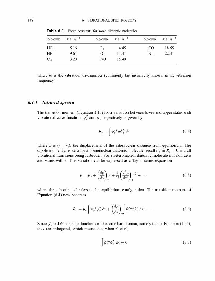
where o is the vibration wavenumber (commonly but incorrectly known as the vibration
frequency).
6.1.1 Infrared spectra
The transition moment (Equation 2.13) for a transition between lower and upper states with
vibrational wave functions c00v and c0v respectively is given by
Rv ¼ðcv0*mmc00v dx ð6:4Þ
where x is (r7 re), the displacement of the internuclear distance from equilibrium. The
dipole moment m is zero for a homonuclear diatomic molecule, resulting in Rv ¼ 0 and all
vibrational transitions being forbidden. For a heteronuclear diatomic molecule m is non-zero
and varies with x. This variation can be expressed as a Taylor series expansion
mm ¼ mme þdmmdx
� �e
xþ 1
2!
d2mmdx2
� �e
x2 þ : : : ð6:5Þ
where the subscript ‘e’ refers to the equilibrium configuration. The transition moment of
Equation (6.4) now becomes
Rv ¼ mme
ðcv0*c00v dxþ
dmmdx
� �e
ðcv0*xc00v dxþ : : : ð6:6Þ
Since c0v and c00v are eigenfunctions of the same hamiltonian, namely that in Equation (1.65),
they are orthogonal, which means that, when v0 6¼ v00,
ðcv0*c00v dx ¼ 0 ð6:7Þ
Table 6.1 Force constants for some diatomic molecules
Molecule k=aJ A72 Molecule k=aJ A72 Molecule k=aJ A72
HCl 5.16 F2 4.45 CO 18.55
HF 9.64 O2 11.41 N2 22.41
Cl2 3.20 NO 15.48
138 6 VIBRATIONAL SPECTROSCOPY
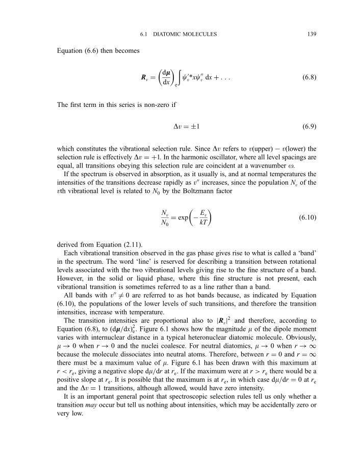
Equation (6.6) then becomes
Rv ¼dmmdx
� �e
ðcv0*xc00v dxþ : : : ð6:8Þ
The first term in this series is non-zero if
Dv ¼ �1 ð6:9Þ
which constitutes the vibrational selection rule. Since Dv refers to v(upper)7 v(lower) theselection rule is effectively Dv ¼ þ1. In the harmonic oscillator, where all level spacings are
equal, all transitions obeying this selection rule are coincident at a wavenumber o.If the spectrum is observed in absorption, as it usually is, and at normal temperatures the
intensities of the transitions decrease rapidly as v00 increases, since the population Nv of the
vth vibrational level is related to N0 by the Boltzmann factor
Nv
N0
¼ exp � Ev
kT
� �ð6:10Þ
derived from Equation (2.11).
Each vibrational transition observed in the gas phase gives rise to what is called a ‘band’
in the spectrum. The word ‘line’ is reserved for describing a transition between rotational
levels associated with the two vibrational levels giving rise to the fine structure of a band.
However, in the solid or liquid phase, where this fine structure is not present, each
vibrational transition is sometimes referred to as a line rather than a band.
All bands with v00 6¼ 0 are referred to as hot bands because, as indicated by Equation
(6.10), the populations of the lower levels of such transitions, and therefore the transition
intensities, increase with temperature.
The transition intensities are proportional also to jRvj2 and therefore, according to
Equation (6.8), to ðdmm=dxÞ2e . Figure 6.1 shows how the magnitude m of the dipole moment
varies with internuclear distance in a typical heteronuclear diatomic molecule. Obviously,
m! 0 when r! 0 and the nuclei coalesce. For neutral diatomics, m! 0 when r!1because the molecule dissociates into neutral atoms. Therefore, between r ¼ 0 and r ¼ 1there must be a maximum value of m. Figure 6.1 has been drawn with this maximum at
r < re, giving a negative slope dm=dr at re. If the maximum were at r > re there would be a
positive slope at re. It is possible that the maximum is at re, in which case dm=dr ¼ 0 at reand the Dv ¼ 1 transitions, although allowed, would have zero intensity.
It is an important general point that spectroscopic selection rules tell us only whether a
transition may occur but tell us nothing about intensities, which may be accidentally zero or
very low.
6.1 DIATOMIC MOLECULES 139
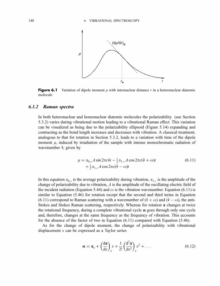
6.1.2 Raman spectra
In both heteronuclear and homonuclear diatomic molecules the polarizability (see Section
5.3.2) varies during vibrational motion leading to a vibrational Raman effect. This variation
can be visualized as being due to the polarizability ellipsoid (Figure 5.14) expanding and
contracting as the bond length increases and decreases with vibration. A classical treatment,
analogous to that for rotation in Section 5.3.2, leads to a variation with time of the dipole
moment m, induced by irradiation of the sample with intense monochromatic radiation of
wavenumber ~nn, given by
m ¼ a0;v A sin 2pc~nnt � 12a1;v A cos 2pcð~nnþ oÞt ð6:11Þ
þ 12a1;v A cos 2pcð~nn� oÞt
In this equation a0;v is the average polarizability during vibration, a1;v is the amplitude of the
change of polarizability due to vibration, A is the amplitude of the oscillating electric field of
the incident radiation (Equation 5.44) and o is the vibration wavenumber. Equation (6.11) is
similar to Equation (5.46) for rotation except that the second and third terms in Equation
(6.11) correspond to Raman scattering with a wavenumber of ð~nnþ oÞ and ð~nn� oÞ, the anti-Stokes and Stokes Raman scattering, respectively. Whereas for rotation aa changes at twice
the rotational frequency, during a complete vibrational cycle a goes through only one cycle
and, therefore, changes at the same frequency as the frequency of vibration. This accounts
for the absence of the factor of two in Equation (6.11) compared with Equation (5.46).
As for the change of dipole moment, the change of polarizability with vibrational
displacement x can be expressed as a Taylor series
a ¼ aae þdaadx
� �e
xþ 1
2!
d2aadx2
� �e
x2 þ : : : ð6:12Þ
Figure 6.1 Variation of dipole moment m with internuclear distance r in a heteronuclear diatomic
molecule
140 6 VIBRATIONAL SPECTROSCOPY
By analogy with Equation (6.6) the vibrational Raman transition moment Rv is given by
Rv ¼daadx
� �e
A
ðcv0*xc00v dxþ : : : ð6:13Þ
and the first term is non-zero only if
Dv ¼ �1 ð6:14Þ
which constitutes the vibrational Raman selection rule. This is the same as for infrared
vibrational transitions, but vibrational Raman spectroscopy has the advantage that
transitions are allowed in homonuclear, as well as heteronuclear, diatomic molecules.
Intensities of Raman transitions are proportional to jRvj2 and therefore, from Equation
(6.13), to ðdaa=dxÞ2e . Since aa is a tensor property we cannot illustrate easily its variation with
x: instead we use the mean polarizability �aa , where
�aa ¼ 13ðaxx þ ayy þ azzÞ ð6:15Þ
Figure 6.2 shows typically how �aa varies with r; d�aa=dr is usually positive and, unlike dm=drin Figure 6.1, varies little with r. For this reason vibrational Raman intensities are less
sensitive than are infrared intensities to the environment of the molecule, such as the solvent
in a solution spectrum.
The mechanism for Stokes and anti-Stokes vibrational Raman transitions is analogous to
that for rotational transitions, illustrated in Figure 5.16. As shown in Figure 6.3, intense
monochromatic radiation may take the molecule from the v ¼ 0 state to a virtual state V0.
Then it may return to v ¼ 0 in a Rayleigh scattering process or to v ¼ 1 in a Stokes Raman
transition. Alternatively, it may go from the v ¼ 1 state to the virtual state V1 and return to
v ¼ 1 (Rayleigh) or to v ¼ 0 (Raman anti-Stokes). However, in many molecules at normal
Figure 6.2 Variation of the mean polarizability �aa with internuclear distance r in a diatomic
molecule
6.1 DIATOMIC MOLECULES 141
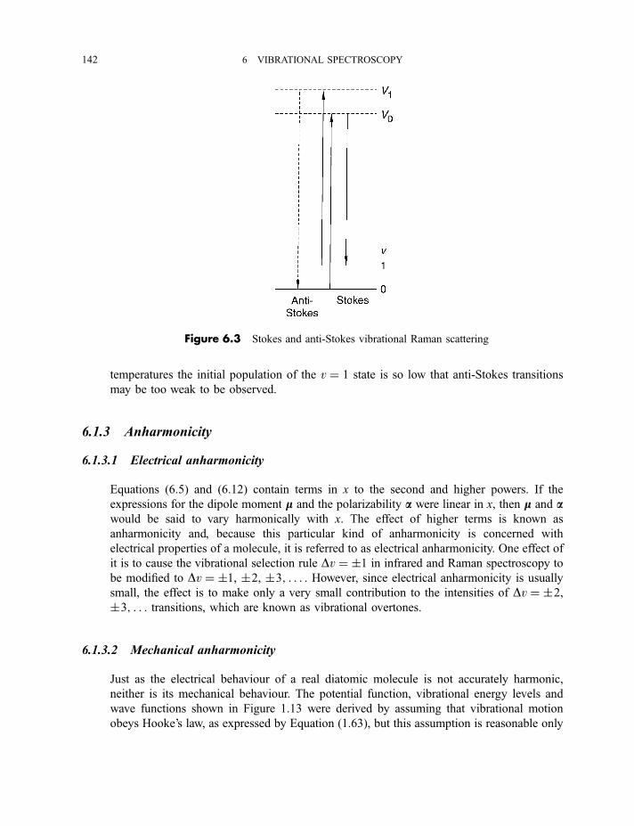
temperatures the initial population of the v ¼ 1 state is so low that anti-Stokes transitions
may be too weak to be observed.
6.1.3 Anharmonicity
6.1.3.1 Electrical anharmonicity
Equations (6.5) and (6.12) contain terms in x to the second and higher powers. If the
expressions for the dipole moment mm and the polarizability aa were linear in x, then mm and aawould be said to vary harmonically with x. The effect of higher terms is known as
anharmonicity and, because this particular kind of anharmonicity is concerned with
electrical properties of a molecule, it is referred to as electrical anharmonicity. One effect of
it is to cause the vibrational selection rule Dv ¼ �1 in infrared and Raman spectroscopy to
be modified to Dv ¼ �1, �2, �3; . . . . However, since electrical anharmonicity is usually
small, the effect is to make only a very small contribution to the intensities of Dv ¼ �2,�3; . . . transitions, which are known as vibrational overtones.
6.1.3.2 Mechanical anharmonicity
Just as the electrical behaviour of a real diatomic molecule is not accurately harmonic,
neither is its mechanical behaviour. The potential function, vibrational energy levels and
wave functions shown in Figure 1.13 were derived by assuming that vibrational motion
obeys Hooke’s law, as expressed by Equation (1.63), but this assumption is reasonable only
Figure 6.3 Stokes and anti-Stokes vibrational Raman scattering
142 6 VIBRATIONAL SPECTROSCOPY
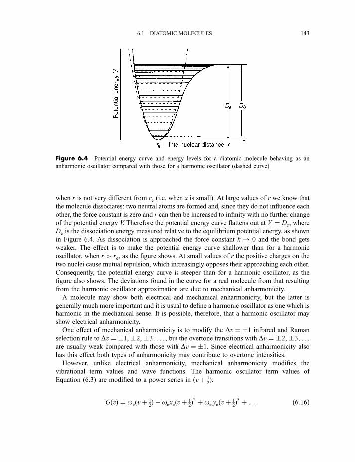
when r is not very different from re (i.e. when x is small). At large values of r we know that
the molecule dissociates: two neutral atoms are formed and, since they do not influence each
other, the force constant is zero and r can then be increased to infinity with no further change
of the potential energy V. Therefore the potential energy curve flattens out at V ¼ De, where
De is the dissociation energy measured relative to the equilibrium potential energy, as shown
in Figure 6.4. As dissociation is approached the force constant k ! 0 and the bond gets
weaker. The effect is to make the potential energy curve shallower than for a harmonic
oscillator, when r > re, as the figure shows. At small values of r the positive charges on the
two nuclei cause mutual repulsion, which increasingly opposes their approaching each other.
Consequently, the potential energy curve is steeper than for a harmonic oscillator, as the
figure also shows. The deviations found in the curve for a real molecule from that resulting
from the harmonic oscillator approximation are due to mechanical anharmonicity.
A molecule may show both electrical and mechanical anharmonicity, but the latter is
generally much more important and it is usual to define a harmonic oscillator as one which is
harmonic in the mechanical sense. It is possible, therefore, that a harmonic oscillator may
show electrical anharmonicity.
One effect of mechanical anharmonicity is to modify the Dv ¼ �1 infrared and Raman
selection rule to Dv ¼ �1, �2, �3; . . . , but the overtone transitions with Dv ¼ �2, �3; . . .are usually weak compared with those with Dv ¼ �1. Since electrical anharmonicity also
has this effect both types of anharmonicity may contribute to overtone intensities.
However, unlike electrical anharmonicity, mechanical anharmonicity modifies the
vibrational term values and wave functions. The harmonic oscillator term values of
Equation (6.3) are modified to a power series in ðvþ 12):
GðvÞ ¼ oeðvþ 12Þ � oexeðvþ 1
2Þ2 þ oe yeðvþ 1
2Þ3 þ : : : ð6:16Þ
Figure 6.4 Potential energy curve and energy levels for a diatomic molecule behaving as an
anharmonic oscillator compared with those for a harmonic oscillator (dashed curve)
6.1 DIATOMIC MOLECULES 143
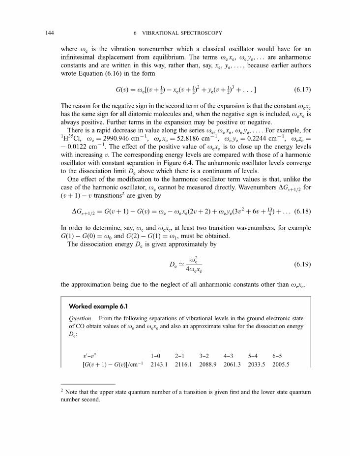
where oe is the vibration wavenumber which a classical oscillator would have for an
infinitesimal displacement from equilibrium. The terms oe xe, oe ye; . . . are anharmonic
constants and are written in this way, rather than, say, xe, ye; . . . , because earlier authors
wrote Equation (6.16) in the form
GðvÞ ¼ oe½ðvþ 12Þ � xeðvþ 1
2Þ2 þ yeðvþ 1
2Þ3 þ : : : � ð6:17Þ
The reason for the negative sign in the second term of the expansion is that the constant oexehas the same sign for all diatomic molecules and, when the negative sign is included, oexe is
always positive. Further terms in the expansion may be positive or negative.
There is a rapid decrease in value along the series oe, oe xe, oe ye; . . . . For example, for1H35Cl, oe ¼ 2990.946 cm71, oe xe ¼ 52.8186 cm71, oe ye ¼ 0.2244 cm71, oeze ¼7 0.0122 cm71. The effect of the positive value of oexe is to close up the energy levels
with increasing v. The corresponding energy levels are compared with those of a harmonic
oscillator with constant separation in Figure 6.4. The anharmonic oscillator levels converge
to the dissociation limit De above which there is a continuum of levels.
One effect of the modification to the harmonic oscillator term values is that, unlike the
case of the harmonic oscillator, oe cannot be measured directly. Wavenumbers DGvþ1=2 forðvþ 1Þ � v transitions2 are given by
DGvþ1=2 ¼ Gðvþ 1Þ � GðvÞ ¼ oe � oe xeð2vþ 2Þ þ oe yeð3v2 þ 6vþ 134Þ þ . . . ð6:18Þ
In order to determine, say, oe and oexe, at least two transition wavenumbers, for example
Gð1Þ � Gð0Þ ¼ o0 and Gð2Þ � Gð1Þ ¼ o1, must be obtained.
The dissociation energy De is given approximately by
De ’o2
e
4oexeð6:19Þ
the approximation being due to the neglect of all anharmonic constants other than oexe.
Worked example 6.1
Question. From the following separations of vibrational levels in the ground electronic state
of CO obtain values of oe and oexe and also an approximate value for the dissociation energy
De:
v0--v00
½Gðvþ 1Þ � GðvÞ�=cm�11--0
2143:1
2--1
2116:1
3--2
2088:9
4--3
2061:3
5--4
2033:5
6--5
2005:5
2 Note that the upper state quantum number of a transition is given first and the lower state quantum
number second.
144 6 VIBRATIONAL SPECTROSCOPY
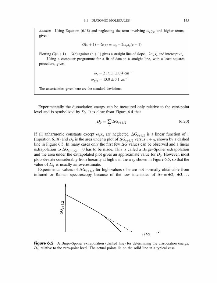
Answer. Using Equation (6.18) and neglecting the term involving oe ye, and higher terms,
gives
Gðvþ 1Þ � GðvÞ ¼ oe � 2oexeðvþ 1Þ
Plotting Gðvþ 1Þ � GðvÞ against ðvþ 1Þ gives a straight line of slope �2oexe and intercept oe.
Using a computer programme for a fit of data to a straight line, with a least squares
procedure, gives
oe ¼ 2171:1� 0:4 cm�1
oexe ¼ 13:8� 0:1 cm�1
The uncertainties given here are the standard deviations.
Experimentally the dissociation energy can be measured only relative to the zero-point
level and is symbolized by D0. It is clear from Figure 6.4 that
D0 ¼PvDGvþ1=2 ð6:20Þ
If all anharmonic constants except oexe are neglected, DGvþ1=2 is a linear function of v(Equation 6.18) and D0 is the area under a plot of DGvþ1=2 versus vþ 1
2, shown by a dashed
line in Figure 6.5. In many cases only the first few DG values can be observed and a linear
extrapolation to DGvþ1=2 ¼ 0 has to be made. This is called a Birge–Sponer extrapolation
and the area under the extrapolated plot gives an approximate value for D0. However, most
plots deviate considerably from linearity at high v in the way shown in Figure 6.5, so that thevalue of D0 is usually an overestimate.
Experimental values of DGvþ1=2 for high values of v are not normally obtainable from
infrared or Raman spectroscopy because of the low intensities of Dv ¼ �2, �3; . . .
Figure 6.5 A Birge–Sponer extrapolation (dashed line) for determining the dissociation energy,
D0, relative to the zero-point level. The actual points lie on the solid line in a typical case
6.1 DIATOMIC MOLECULES 145
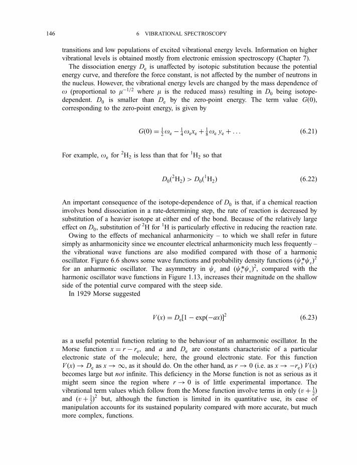
transitions and low populations of excited vibrational energy levels. Information on higher
vibrational levels is obtained mostly from electronic emission spectroscopy (Chapter 7).
The dissociation energy De is unaffected by isotopic substitution because the potential
energy curve, and therefore the force constant, is not affected by the number of neutrons in
the nucleus. However, the vibrational energy levels are changed by the mass dependence of
o (proportional to m�1=2 where m is the reduced mass) resulting in D0 being isotope-
dependent. D0 is smaller than De by the zero-point energy. The term value Gð0Þ,corresponding to the zero-point energy, is given by
Gð0Þ ¼ 12oe � 1
4oexe þ 1
8oe ye þ . . . ð6:21Þ
For example, oe for2H2 is less than that for 1H2 so that
D0ð2H2Þ > D0ð1H2Þ ð6:22Þ
An important consequence of the isotope-dependence of D0 is that, if a chemical reaction
involves bond dissociation in a rate-determining step, the rate of reaction is decreased by
substitution of a heavier isotope at either end of the bond. Because of the relatively large
effect on D0, substitution of 2H for 1H is particularly effective in reducing the reaction rate.
Owing to the effects of mechanical anharmonicity – to which we shall refer in future
simply as anharmonicity since we encounter electrical anharmonicity much less frequently –
the vibrational wave functions are also modified compared with those of a harmonic
oscillator. Figure 6.6 shows some wave functions and probability density functions ðcv*cvÞ2for an anharmonic oscillator. The asymmetry in cv and ðcv*cvÞ2, compared with the
harmonic oscillator wave functions in Figure 1.13, increases their magnitude on the shallow
side of the potential curve compared with the steep side.
In 1929 Morse suggested
V ðxÞ ¼ De½1� expð�axÞ�2 ð6:23Þ
as a useful potential function relating to the behaviour of an anharmonic oscillator. In the
Morse function x ¼ r � re, and a and De are constants characteristic of a particular
electronic state of the molecule; here, the ground electronic state. For this function
V ðxÞ ! De as x!1, as it should do. On the other hand, as r! 0 (i.e. as x!�re) V ðxÞbecomes large but not infinite. This deficiency in the Morse function is not as serious as it
might seem since the region where r! 0 is of little experimental importance. The
vibrational term values which follow from the Morse function involve terms in only ðvþ 12Þ
and ðvþ 12Þ2 but, although the function is limited in its quantitative use, its ease of
manipulation accounts for its sustained popularity compared with more accurate, but much
more complex, functions.
146 6 VIBRATIONAL SPECTROSCOPY
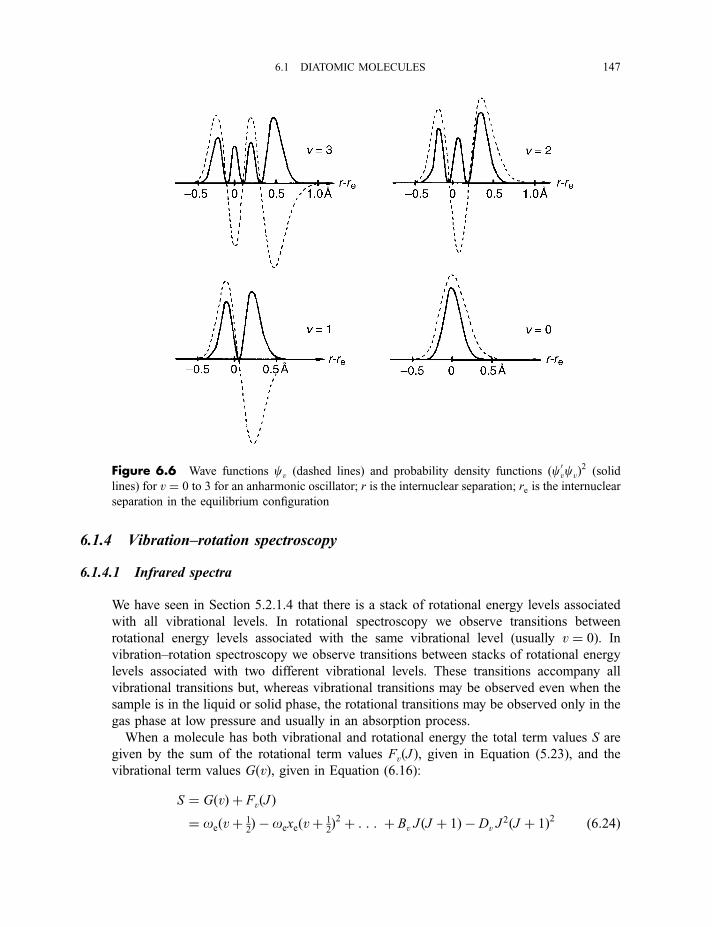
6.1.4 Vibration–rotation spectroscopy
6.1.4.1 Infrared spectra
We have seen in Section 5.2.1.4 that there is a stack of rotational energy levels associated
with all vibrational levels. In rotational spectroscopy we observe transitions between
rotational energy levels associated with the same vibrational level (usually v ¼ 0). In
vibration–rotation spectroscopy we observe transitions between stacks of rotational energy
levels associated with two different vibrational levels. These transitions accompany all
vibrational transitions but, whereas vibrational transitions may be observed even when the
sample is in the liquid or solid phase, the rotational transitions may be observed only in the
gas phase at low pressure and usually in an absorption process.
When a molecule has both vibrational and rotational energy the total term values S are
given by the sum of the rotational term values FvðJ Þ, given in Equation (5.23), and the
vibrational term values GðvÞ, given in Equation (6.16):
S ¼ GðvÞ þ FvðJ Þ¼ oeðvþ 1
2Þ � oexeðvþ 1
2Þ2 þ : : : þ Bv J ðJ þ 1Þ � Dv J
2ðJ þ 1Þ2 ð6:24Þ
Figure 6.6 Wave functions cv (dashed lines) and probability density functions ðc0vcvÞ2 (solid
lines) for v ¼ 0 to 3 for an anharmonic oscillator; r is the internuclear separation; re is the internuclear
separation in the equilibrium configuration
6.1 DIATOMIC MOLECULES 147
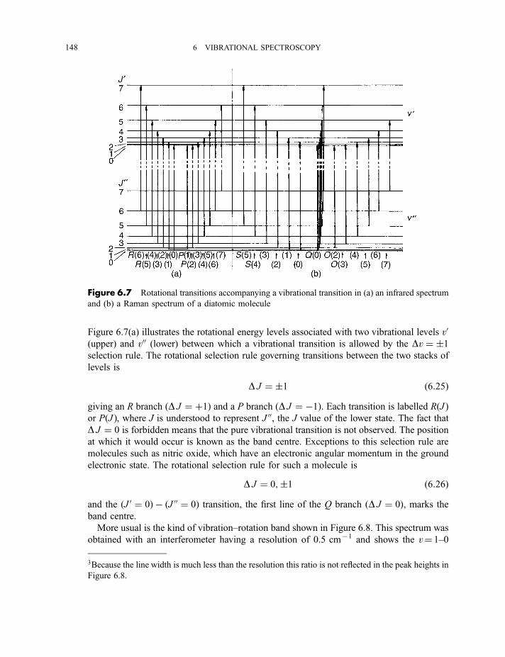
Figure 6.7(a) illustrates the rotational energy levels associated with two vibrational levels v0(upper) and v00 (lower) between which a vibrational transition is allowed by the Dv ¼ �1selection rule. The rotational selection rule governing transitions between the two stacks of
levels is
D J ¼ �1 ð6:25Þgiving an R branch ðD J ¼ þ1Þ and a P branch ðD J ¼ �1Þ. Each transition is labelled RðJ Þor PðJ Þ, where J is understood to represent J 00, the J value of the lower state. The fact that
D J ¼ 0 is forbidden means that the pure vibrational transition is not observed. The position
at which it would occur is known as the band centre. Exceptions to this selection rule are
molecules such as nitric oxide, which have an electronic angular momentum in the ground
electronic state. The rotational selection rule for such a molecule is
D J ¼ 0;�1 ð6:26Þand the ðJ 0 ¼ 0Þ � ðJ 00 ¼ 0Þ transition, the first line of the Q branch ðD J ¼ 0Þ, marks the
band centre.
More usual is the kind of vibration–rotation band shown in Figure 6.8. This spectrum was
obtained with an interferometer having a resolution of 0.5 cm71 and shows the v¼ 1–0
Figure 6.7 Rotational transitions accompanying a vibrational transition in (a) an infrared spectrum
and (b) a Raman spectrum of a diatomic molecule
3Because the line width is much less than the resolution this ratio is not reflected in the peak heights in
Figure 6.8.
148 6 VIBRATIONAL SPECTROSCOPY
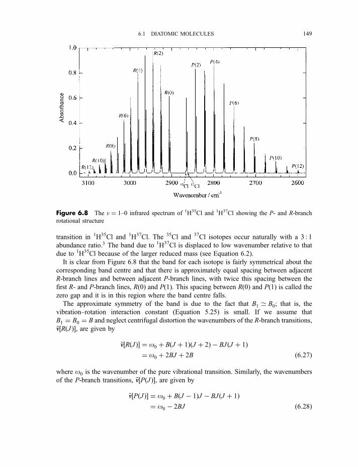
transition in 1H35Cl and 1H37Cl. The 35Cl and 37Cl isotopes occur naturally with a 3 : 1
abundance ratio.3 The band due to 1H37Cl is displaced to low wavenumber relative to that
due to 1H35Cl because of the larger reduced mass (see Equation 6.2).
It is clear from Figure 6.8 that the band for each isotope is fairly symmetrical about the
corresponding band centre and that there is approximately equal spacing between adjacent
R-branch lines and between adjacent P-branch lines, with twice this spacing between the
first R- and P-branch lines, R(0) and P(1). This spacing between R(0) and P(1) is called the
zero gap and it is in this region where the band centre falls.
The approximate symmetry of the band is due to the fact that B1 ’ B0; that is, the
vibration–rotation interaction constant (Equation 5.25) is small. If we assume that
B1 ¼ B0 ¼ B and neglect centrifugal distortion the wavenumbers of the R-branch transitions,
~nn½RðJ Þ�, are given by
~nn½RðJ Þ� ¼ o0 þ BðJ þ 1ÞðJ þ 2Þ � BJ ðJ þ 1Þ¼ o0 þ 2BJ þ 2B ð6:27Þ
where o0 is the wavenumber of the pure vibrational transition. Similarly, the wavenumbers
of the P-branch transitions, ~nn½PðJ Þ�, are given by
~nn½PðJ Þ� ¼ o0 þ BðJ � 1ÞJ � BJ ðJ þ 1Þ¼ o0 � 2BJ ð6:28Þ
Figure 6.8 The v ¼ 1–0 infrared spectrum of 1H35Cl and 1H37Cl showing the P- and R-branch
rotational structure
6.1 DIATOMIC MOLECULES 149
From Equations (6.27) and (6.28) it follows that the zero gap, ~nn½Rð0Þ� � ~nn½Pð1Þ�, is 4B and
that the spacing is 2B between adjacent R-branch lines and also between adjacent P-branch
lines, hence the approximate symmetry of the band.
A close look at Figure 6.8 reveals that the band is not quite symmetrical but shows a
convergence in the R branch and a divergence in the P branch. This behaviour is due
principally to the inequality of B0 and B1 and there is sufficient information in the band to be
able to determine these two quantities separately. The method used is called the method of
combination differences which employs a principle quite common in spectroscopy. The
principle is that, if we wish to derive information about a series of lower states and a series of
upper states, between which transitions are occurring, then differences in wavenumber
between transitions with a common upper state are dependent on properties of the lower
states only. Similarly, differences in wavenumber between transitions with a common lower
state are dependent on properties of the upper states only.
In the case of a vibration–rotation band it is clear from Figure 6.7(a) that, since Rð0Þ andPð2Þ have a common upper state with J 0 ¼ 1, then ~nn½Rð0Þ� � ~nn½Pð2Þ� must be a function of
B00 only. The transitions Rð1Þ and Pð3Þ have J 0 ¼ 2 in common and, in general,
~nn½RðJ � 1Þ� � ~nn½PðJ þ 1Þ�, usually written as D002FðJ Þ,4 is a function of B00 only. If we
continue to neglect centrifugal distortion the function is given by
D002FðJ Þ ¼ ~nn½RðJ � 1Þ� � ~nn½PðJ þ 1Þ�¼ o0 þ B0J ðJ þ 1Þ � B00ðJ � 1ÞJ� ½o0 þ B0J ðJ þ 1Þ � B00ðJ þ 1ÞðJ þ 2Þ�¼ 4B00ðJ þ 1
2Þ ð6:29Þ
After assignment and measurement of the wavenumbers of the rotational lines a graph of
D002FðJ Þ versus ðJ þ 12Þ is a straight line of slope 4B00.
Similarly, since all pairs of transitions RðJ Þ and PðJ Þ have common lower states,
~nn½RðJ Þ� � ~nn½PðJ Þ� is a function of B0 only and we have
D02FðJ Þ ¼ ~nn½RðJ Þ� � ~nn½PðJ Þ�¼ o0 þ B0ðJ þ 1ÞðJ þ 2Þ � B00J ðJ þ 1Þ� ½o0 þ B0ðJ � 1ÞJ � B00J ðJ þ 1Þ�¼ 4B0ðJ þ 1
2Þ ð6:30Þ
and a graph of D02FðJ Þ versus ðJ þ 12Þ is a straight line of slope 4B0.
The band centre is not quite midway between Rð0Þ and Pð1Þ but its wavenumber o0 can be
obtained from
o0 ¼ ~nn½Rð0Þ� � 2B0 ð6:31Þ¼ ~nn½Pð1Þ� þ 2B00
4 The reason for the subscript 2 in the D002FðJ Þ symbol is that these are the differences between
rotational term values, in a particular vibrational state, with J differing by 2.
150 6 VIBRATIONAL SPECTROSCOPY
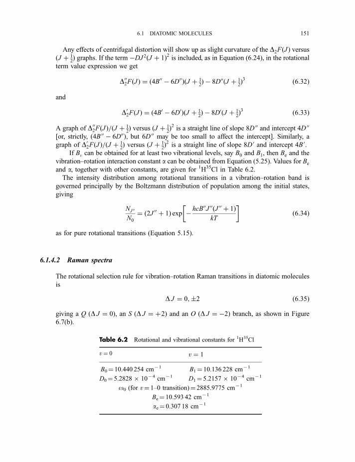
Any effects of centrifugal distortion will show up as slight curvature of the D2FðJ Þ versusðJ þ 1
2Þ graphs. If the term �DJ 2ðJ þ 1Þ2 is included, as in Equation (6.24), in the rotational
term value expression we get
D002FðJ Þ ¼ ð4B00 � 6D00ÞðJ þ 12Þ � 8D00ðJ þ 1
2Þ3 ð6:32Þ
and
D02FðJ Þ ¼ ð4B0 � 6D0ÞðJ þ 12Þ � 8D0ðJ þ 1
2Þ3 ð6:33Þ
A graph of D002FðJ Þ=ðJ þ 12Þ versus ðJ þ 1
2Þ2 is a straight line of slope 8D 00 and intercept 4D 00
[or, strictly, ð4B 00 � 6D00Þ, but 6D 00 may be too small to affect the intercept]. Similarly, a
graph of D02FðJ Þ=ðJ þ 12Þ versus ðJ þ 1
2Þ2 is a straight line of slope 8D 0 and intercept 4B 0.
If Bv can be obtained for at least two vibrational levels, say B0 and B1, then Be and the
vibration–rotation interaction constant a can be obtained from Equation (5.25). Values for Be
and a, together with other constants, are given for 1H35Cl in Table 6.2.
The intensity distribution among rotational transitions in a vibration–rotation band is
governed principally by the Boltzmann distribution of population among the initial states,
giving
NJ 00
N0
¼ ð2J 00 þ 1Þ exp � hcB00J 00ðJ 00 þ 1ÞkT
� �ð6:34Þ
as for pure rotational transitions (Equation 5.15).
6.1.4.2 Raman spectra
The rotational selection rule for vibration–rotation Raman transitions in diatomic molecules
is
D J ¼ 0;�2 ð6:35Þ
giving a Q ðD J ¼ 0Þ, an S ðD J ¼ þ2Þ and an O ðD J ¼ �2Þ branch, as shown in Figure
6.7(b).
Table 6.2 Rotational and vibrational constants for 1H35Cl
v ¼ 0 v ¼ 1
B0¼ 10.440 254 cm71 B1¼ 10.136 228 cm71
D0¼ 5.28286 1074 cm71 D1¼ 5.21576 1074 cm71
o0 (for v¼ 1–0 transition)¼ 2885.9775 cm71
Be¼ 10.593 42 cm71
ae¼ 0.307 18 cm71
6.1 DIATOMIC MOLECULES 151
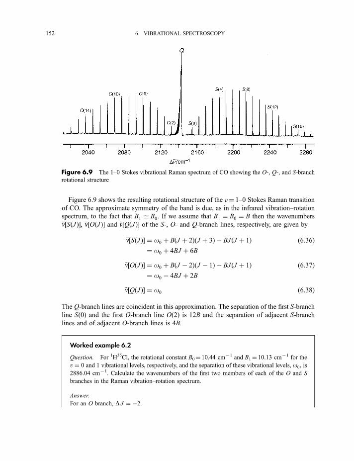
Figure 6.9 shows the resulting rotational structure of the v¼ 1–0 Stokes Raman transition
of CO. The approximate symmetry of the band is due, as in the infrared vibration–rotation
spectrum, to the fact that B1 ’ B0. If we assume that B1 ¼ B0 ¼ B then the wavenumbers
~nn½SðJ Þ�, ~nn½OðJ Þ� and ~nn½QðJ Þ� of the S-, O- and Q-branch lines, respectively, are given by
~nn½SðJ Þ� ¼ o0 þ BðJ þ 2ÞðJ þ 3Þ � BJ ðJ þ 1Þ ð6:36Þ¼ o0 þ 4BJ þ 6B
~nn½OðJ Þ� ¼ o0 þ BðJ � 2ÞðJ � 1Þ � BJ ðJ þ 1Þ ð6:37Þ¼ o0 � 4BJ þ 2B
~nn½QðJ Þ� ¼ o0 ð6:38Þ
The Q-branch lines are coincident in this approximation. The separation of the first S-branch
line Sð0Þ and the first O-branch line Oð2Þ is 12B and the separation of adjacent S-branch
lines and of adjacent O-branch lines is 4B.
Worked example 6.2
Question. For 1H35Cl, the rotational constant B0¼ 10.44 cm71 and B1¼ 10.13 cm71 for the
v ¼ 0 and 1 vibrational levels, respectively, and the separation of these vibrational levels, o0, is
2886.04 cm71. Calculate the wavenumbers of the first two members of each of the O and S
branches in the Raman vibration–rotation spectrum.
Answer.
For an O branch, D J ¼ �2.
Figure 6.9 The 1–0 Stokes vibrational Raman spectrum of CO showing the O-, Q-, and S-branch
rotational structure
152 6 VIBRATIONAL SPECTROSCOPY
; For the first line, J 00 ¼ 2 (lower state) and J 0 ¼ 0 (upper state)
; ~nn½Oð2Þ� ¼ o0 þ B0J 0ðJ 0 þ 1Þ � B00J 00ðJ 00 þ 1Þ¼ o0 þ 0� 6B0
¼ 2823:40 cm�1
and, for the second line, J 00 ¼ 3 and J 0 ¼ 1
; ~nn½Oð3Þ� ¼ o0 þ 2B1 � 12B0
¼ 2781:02 cm�1
For an S branch, D J ¼ þ2.; For the first line, J 00 ¼ 0 and J 0 ¼ 2
; ~nn½Sð0Þ� ¼ o0 þ B0J 0ðJ 0 þ 1Þ � B00J 00ðJ 00 þ 1Þ¼ o0 þ 6B1 � 0
¼ 2946:82 cm�1
and, for the second line, J 00 ¼ 1 and J 0 ¼ 3
; ~nn½Sð1Þ� ¼ o0 þ 12B1 � 2B0
¼ 2986:72 cm�1
More accurately, we can use the method of combination differences, while still neglecting
centrifugal distortion, to obtain B00 and B0. Transitions having wavenumbers ~nn½SðJ � 2Þ� and~nn½OðJ þ 2Þ� have a common upper state so that the corresponding combination difference
D004FðJ Þ is a function of B00 only:
D04FðJ Þ ¼ ~nn½SðJ � 2Þ� � ~nn½OðJ þ 2Þ� ¼ 8B00ðJ þ 12Þ ð6:39Þ
Similarly, transitions having wavenumbers ~nn½SðJ Þ� and ~nn½OðJ Þ� have a common lower state
and
D004FðJ Þ ¼ ~nn½SðJ Þ� � ~nn½OðJ Þ� ¼ 8B0ðJ þ 12Þ ð6:40Þ
Plotting a graph of D004FðJ Þ versus ðJ þ 12Þ and D04FðJ Þ versus ðJ þ 1
2Þ gives straight lines with
slopes 8B00 and 8B0, respectively.Nuclear spin statistical weights were discussed in Section 5.3.4 and the effects on the
populations of the rotational levels in the v ¼ 0 states of 1H2,19F2,
2H2,14N2 and 16O2
illustrated as examples in Figure 5.18. The effect of these statistical weights in the vibration–
rotation Raman spectra is to cause a J 00 even : odd intensity alternation of 1 : 3 for 1H2 and19F2 and 6 : 3 for 2H2 and
14N2; for16O2, all transitions with J 00 even are absent. It is for the
6.1 DIATOMIC MOLECULES 153
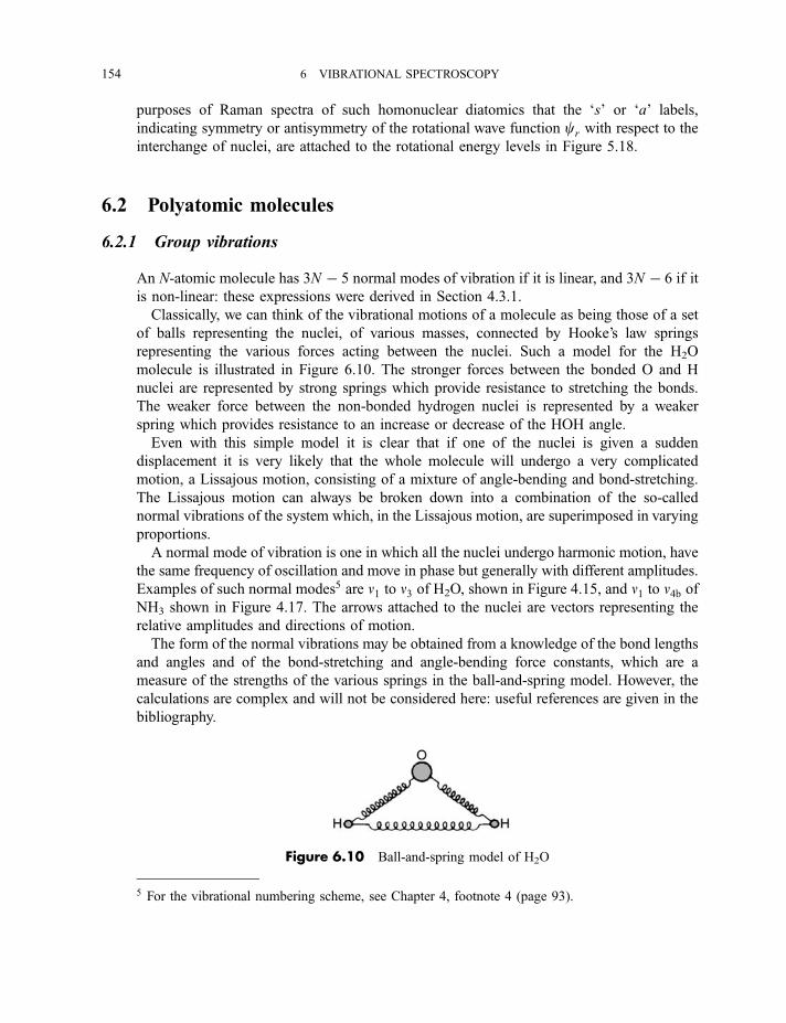
purposes of Raman spectra of such homonuclear diatomics that the ‘s’ or ‘a’ labels,
indicating symmetry or antisymmetry of the rotational wave function cr with respect to the
interchange of nuclei, are attached to the rotational energy levels in Figure 5.18.
6.2 Polyatomic molecules
6.2.1 Group vibrations
An N-atomic molecule has 3N � 5 normal modes of vibration if it is linear, and 3N � 6 if it
is non-linear: these expressions were derived in Section 4.3.1.
Classically, we can think of the vibrational motions of a molecule as being those of a set
of balls representing the nuclei, of various masses, connected by Hooke’s law springs
representing the various forces acting between the nuclei. Such a model for the H2O
molecule is illustrated in Figure 6.10. The stronger forces between the bonded O and H
nuclei are represented by strong springs which provide resistance to stretching the bonds.
The weaker force between the non-bonded hydrogen nuclei is represented by a weaker
spring which provides resistance to an increase or decrease of the HOH angle.
Even with this simple model it is clear that if one of the nuclei is given a sudden
displacement it is very likely that the whole molecule will undergo a very complicated
motion, a Lissajous motion, consisting of a mixture of angle-bending and bond-stretching.
The Lissajous motion can always be broken down into a combination of the so-called
normal vibrations of the system which, in the Lissajous motion, are superimposed in varying
proportions.
A normal mode of vibration is one in which all the nuclei undergo harmonic motion, have
the same frequency of oscillation and move in phase but generally with different amplitudes.
Examples of such normal modes5 are n1 to n3 of H2O, shown in Figure 4.15, and n1 to n4b ofNH3 shown in Figure 4.17. The arrows attached to the nuclei are vectors representing the
relative amplitudes and directions of motion.
The form of the normal vibrations may be obtained from a knowledge of the bond lengths
and angles and of the bond-stretching and angle-bending force constants, which are a
measure of the strengths of the various springs in the ball-and-spring model. However, the
calculations are complex and will not be considered here: useful references are given in the
bibliography.
Figure 6.10 Ball-and-spring model of H2O
5 For the vibrational numbering scheme, see Chapter 4, footnote 4 (page 93).
154 6 VIBRATIONAL SPECTROSCOPY
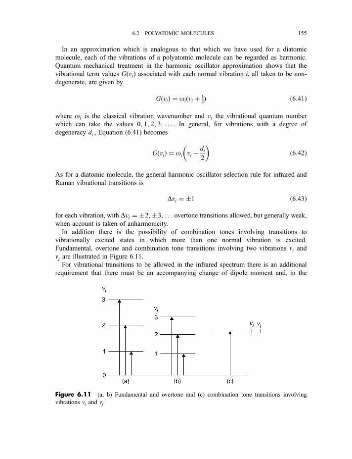
In an approximation which is analogous to that which we have used for a diatomic
molecule, each of the vibrations of a polyatomic molecule can be regarded as harmonic.
Quantum mechanical treatment in the harmonic oscillator approximation shows that the
vibrational term values GðviÞ associated with each normal vibration i, all taken to be non-
degenerate, are given by
GðviÞ ¼ oiðvi þ 12Þ ð6:41Þ
where oi is the classical vibration wavenumber and vi the vibrational quantum number
which can take the values 0; 1; 2; 3; . . . . In general, for vibrations with a degree of
degeneracy di , Equation (6.41) becomes
GðviÞ ¼ oi vi þdi
2
� �ð6:42Þ
As for a diatomic molecule, the general harmonic oscillator selection rule for infrared and
Raman vibrational transitions is
Dvi ¼ �1 ð6:43Þ
for each vibration, with Dvi ¼ �2, �3; . . . overtone transitions allowed, but generally weak,when account is taken of anharmonicity.
In addition there is the possibility of combination tones involving transitions to
vibrationally excited states in which more than one normal vibration is excited.
Fundamental, overtone and combination tone transitions involving two vibrations ni andnj are illustrated in Figure 6.11.
For vibrational transitions to be allowed in the infrared spectrum there is an additional
requirement that there must be an accompanying change of dipole moment and, in the
Figure 6.11 (a, b) Fundamental and overtone and (c) combination tone transitions involving
vibrations ni and nj
6.2 POLYATOMIC MOLECULES 155
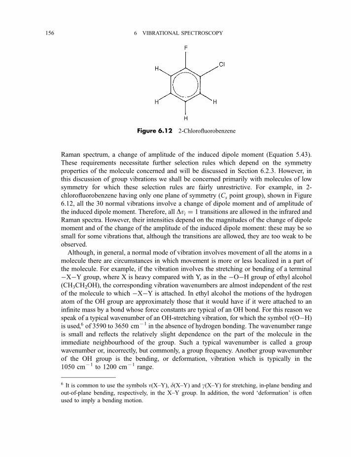
Raman spectrum, a change of amplitude of the induced dipole moment (Equation 5.43).
These requirements necessitate further selection rules which depend on the symmetry
properties of the molecule concerned and will be discussed in Section 6.2.3. However, in
this discussion of group vibrations we shall be concerned primarily with molecules of low
symmetry for which these selection rules are fairly unrestrictive. For example, in 2-
chlorofluorobenzene having only one plane of symmetry (Cs point group), shown in Figure
6.12, all the 30 normal vibrations involve a change of dipole moment and of amplitude of
the induced dipole moment. Therefore, all Dvi ¼ 1 transitions are allowed in the infrared and
Raman spectra. However, their intensities depend on the magnitudes of the change of dipole
moment and of the change of the amplitude of the induced dipole moment: these may be so
small for some vibrations that, although the transitions are allowed, they are too weak to be
observed.
Although, in general, a normal mode of vibration involves movement of all the atoms in a
molecule there are circumstances in which movement is more or less localized in a part of
the molecule. For example, if the vibration involves the stretching or bending of a terminal
�X�Y group, where X is heavy compared with Y, as in the �O�H group of ethyl alcohol
(CH3CH2OH), the corresponding vibration wavenumbers are almost independent of the rest
of the molecule to which �X�Y is attached. In ethyl alcohol the motions of the hydrogen
atom of the OH group are approximately those that it would have if it were attached to an
infinite mass by a bond whose force constants are typical of an OH bond. For this reason we
speak of a typical wavenumber of an OH-stretching vibration, for which the symbol n(O�H)is used,6 of 3590 to 3650 cm71 in the absence of hydrogen bonding. The wavenumber range
is small and reflects the relatively slight dependence on the part of the molecule in the
immediate neighbourhood of the group. Such a typical wavenumber is called a group
wavenumber or, incorrectly, but commonly, a group frequency. Another group wavenumber
of the OH group is the bending, or deformation, vibration which is typically in the
1050 cm71 to 1200 cm71 range.
Figure 6.12 2-Chlorofluorobenzene
6 It is common to use the symbols n(X–Y), d(X–Y) and g(X–Y) for stretching, in-plane bending and
out-of-plane bending, respectively, in the X–Y group. In addition, the word ‘deformation’ is often
used to imply a bending motion.
156 6 VIBRATIONAL SPECTROSCOPY
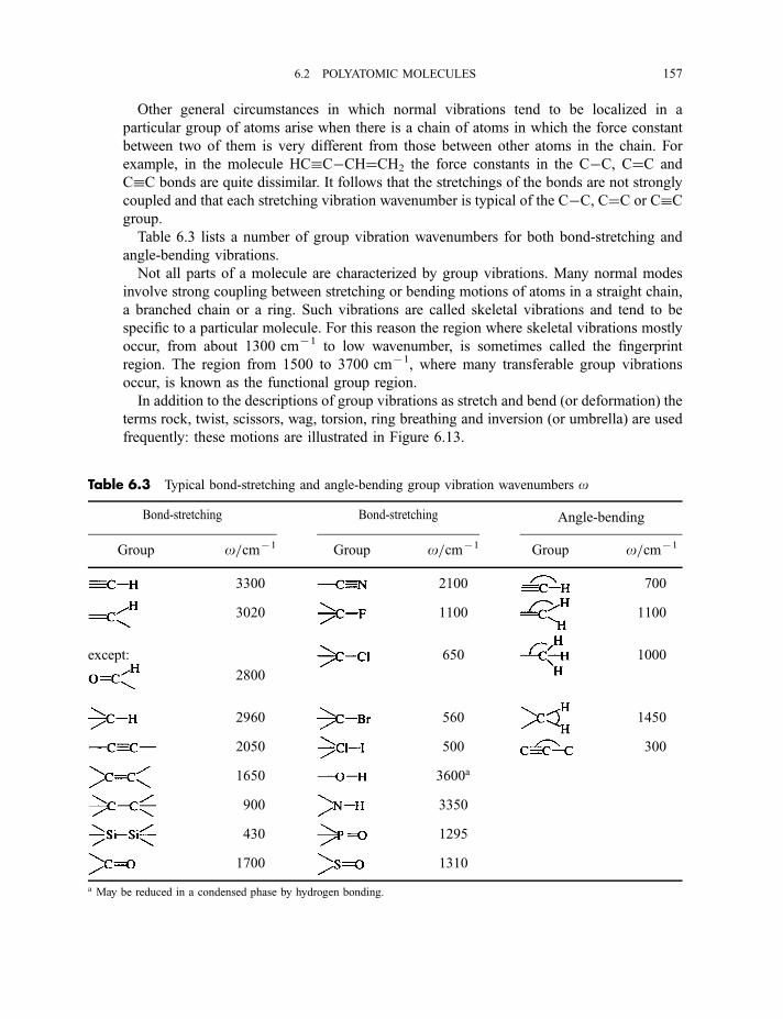
Other general circumstances in which normal vibrations tend to be localized in a
particular group of atoms arise when there is a chain of atoms in which the force constant
between two of them is very different from those between other atoms in the chain. For
example, in the molecule HCC�CH¼CH2 the force constants in the C�C, C¼C and
CC bonds are quite dissimilar. It follows that the stretchings of the bonds are not strongly
coupled and that each stretching vibration wavenumber is typical of the C�C, C¼C or CCgroup.
Table 6.3 lists a number of group vibration wavenumbers for both bond-stretching and
angle-bending vibrations.
Not all parts of a molecule are characterized by group vibrations. Many normal modes
involve strong coupling between stretching or bending motions of atoms in a straight chain,
a branched chain or a ring. Such vibrations are called skeletal vibrations and tend to be
specific to a particular molecule. For this reason the region where skeletal vibrations mostly
occur, from about 1300 cm71 to low wavenumber, is sometimes called the fingerprint
region. The region from 1500 to 3700 cm71, where many transferable group vibrations
occur, is known as the functional group region.
In addition to the descriptions of group vibrations as stretch and bend (or deformation) the
terms rock, twist, scissors, wag, torsion, ring breathing and inversion (or umbrella) are used
frequently: these motions are illustrated in Figure 6.13.
Table 6.3 Typical bond-stretching and angle-bending group vibration wavenumbers o
Bond-stretching Bond-stretching Angle-bending
Group o=cm71 Group o=cm71 Group o=cm71
3300 2100 700
3020 1100 1100
except:
2800
650 1000
2960 560 1450
2050 500 300
1650 3600a
900 3350
430 1295
1700 1310
a May be reduced in a condensed phase by hydrogen bonding.
6.2 POLYATOMIC MOLECULES 157
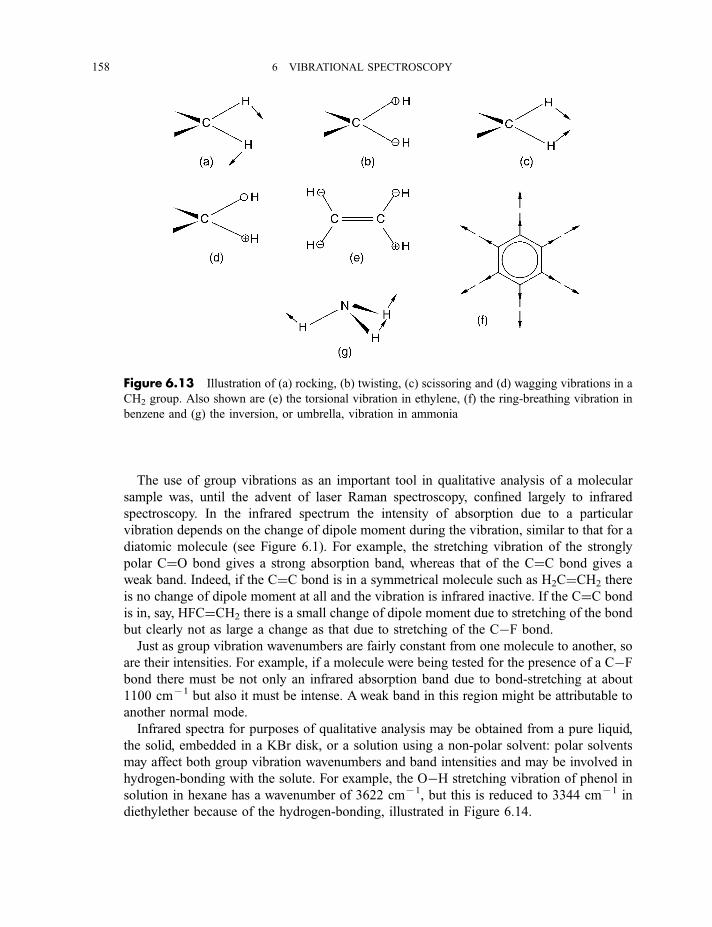
The use of group vibrations as an important tool in qualitative analysis of a molecular
sample was, until the advent of laser Raman spectroscopy, confined largely to infrared
spectroscopy. In the infrared spectrum the intensity of absorption due to a particular
vibration depends on the change of dipole moment during the vibration, similar to that for a
diatomic molecule (see Figure 6.1). For example, the stretching vibration of the strongly
polar C¼O bond gives a strong absorption band, whereas that of the C¼C bond gives a
weak band. Indeed, if the C¼C bond is in a symmetrical molecule such as H2C¼CH2 there
is no change of dipole moment at all and the vibration is infrared inactive. If the C¼C bond
is in, say, HFC¼CH2 there is a small change of dipole moment due to stretching of the bond
but clearly not as large a change as that due to stretching of the C�F bond.
Just as group vibration wavenumbers are fairly constant from one molecule to another, so
are their intensities. For example, if a molecule were being tested for the presence of a C�Fbond there must be not only an infrared absorption band due to bond-stretching at about
1100 cm71 but also it must be intense. A weak band in this region might be attributable to
another normal mode.
Infrared spectra for purposes of qualitative analysis may be obtained from a pure liquid,
the solid, embedded in a KBr disk, or a solution using a non-polar solvent: polar solvents
may affect both group vibration wavenumbers and band intensities and may be involved in
hydrogen-bonding with the solute. For example, the O�H stretching vibration of phenol in
solution in hexane has a wavenumber of 3622 cm71, but this is reduced to 3344 cm71 in
diethylether because of the hydrogen-bonding, illustrated in Figure 6.14.
Figure 6.13 Illustration of (a) rocking, (b) twisting, (c) scissoring and (d) wagging vibrations in a
CH2 group. Also shown are (e) the torsional vibration in ethylene, (f) the ring-breathing vibration in
benzene and (g) the inversion, or umbrella, vibration in ammonia
158 6 VIBRATIONAL SPECTROSCOPY
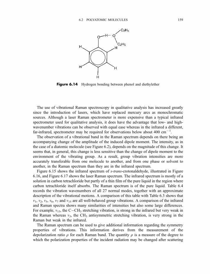
The use of vibrational Raman spectroscopy in qualitative analysis has increased greatly
since the introduction of lasers, which have replaced mercury arcs as monochromatic
sources. Although a laser Raman spectrometer is more expensive than a typical infrared
spectrometer used for qualitative analysis, it does have the advantage that low- and high-
wavenumber vibrations can be observed with equal ease whereas in the infrared a different,
far-infrared, spectrometer may be required for observations below about 400 cm71.
The observation of a vibrational band in the Raman spectrum depends on there being an
accompanying change of the amplitude of the induced dipole moment. The intensity, as in
the case of a diatomic molecule (see Figure 6.2), depends on the magnitude of this change. It
seems that, in general, this change is less sensitive than the change of dipole moment to the
environment of the vibrating group. As a result, group vibration intensities are more
accurately transferable from one molecule to another, and from one phase or solvent to
another, in the Raman spectrum than they are in the infrared spectrum.
Figure 6.15 shows the infrared spectrum of s-trans-crotonaldehyde, illustrated in Figure
6.16, and Figure 6.17 shows the laser Raman spectrum. The infrared spectrum is mostly of a
solution in carbon tetrachloride but partly of a thin film of the pure liquid in the region where
carbon tetrachloride itself absorbs. The Raman spectrum is of the pure liquid. Table 6.4
records the vibration wavenumbers of all 27 normal modes, together with an approximate
description of the vibrational motions. A comparison of this table with Table 6.3 shows that
n1, n2, n5, n6, n7 and n15 are all well-behaved group vibrations. A comparison of the infrared
and Raman spectra shows many similarities of intensities but also some large differences.
For example, n15, the C�CH3 stretching vibration, is strong in the infrared but very weak in
the Raman whereas n3, the CH3 antisymmetric stretching vibration, is very strong in the
Raman but weak in the infrared.
The Raman spectrum can be used to give additional information regarding the symmetry
properties of vibrations. This information derives from the measurement of the
depolarization ratio r for each Raman band. The quantity r is a measure of the degree to
which the polarization properties of the incident radiation may be changed after scattering
Figure 6.14 Hydrogen bonding between phenol and diethylether
6.2 POLYATOMIC MOLECULES 159
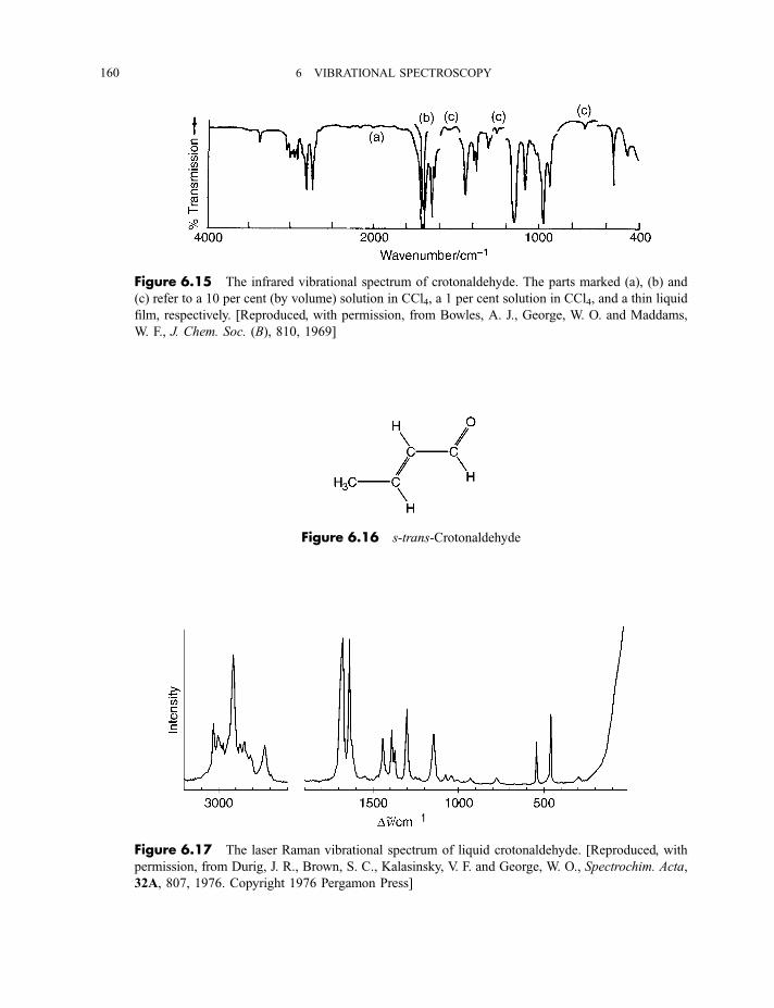
Figure 6.16 s-trans-Crotonaldehyde
Figure 6.17 The laser Raman vibrational spectrum of liquid crotonaldehyde. [Reproduced, with
permission, from Durig, J. R., Brown, S. C., Kalasinsky, V. F. and George, W. O., Spectrochim. Acta,
32A, 807, 1976. Copyright 1976 Pergamon Press]
Figure 6.15 The infrared vibrational spectrum of crotonaldehyde. The parts marked (a), (b) and
(c) refer to a 10 per cent (by volume) solution in CCl4, a 1 per cent solution in CCl4, and a thin liquid
film, respectively. [Reproduced, with permission, from Bowles, A. J., George, W. O. and Maddams,
W. F., J. Chem. Soc. (B), 810, 1969]
160 6 VIBRATIONAL SPECTROSCOPY
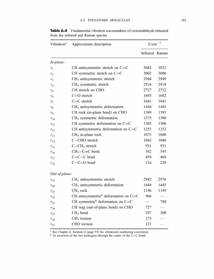
Table 6.4 Fundamental vibration wavenumbers of crotonaldehyde obtained
from the infrared and Raman spectra
Vibrationa Approximate description ~nn=cm71
Infrared Raman
In-plane:
n1 CH antisymmetric stretch on C¼C 3042 3032
n2 CH symmetric stretch on C¼C 3002 3006
n3 CH3 antisymmetric stretch 2944 2949
n4 CH3 symmetric stretch 2916 2918
n5 CH stretch on CHO 2727 2732
n6 C¼O stretch 1693 1682
n7 C¼C stretch 1641 1641
n8 CH3 antisymmetric deformation 1444 1445
n9 CH rock (in-plane bend) on CHO 1389 1393
n10 CH3 symmetric deformation 1375 1380
n11 CH symmetric deformation on C¼C 1305 1306
n12 CH antisymmetric deformation on C¼C 1253 1252
n13 CH3 in-plane rock 1075 1080
n14 C�CHO stretch 1042 1046
n15 C�CH3 stretch 931 931
n16 CH3�C¼C bend 542 545
n17 C¼C�C bend 459 464
n18 C�C¼O bend 216 230
Out-of-plane:
n19 CH3 antisymmetric stretch 2982 2976
n20 CH3 antisymmetric deformation 1444 1445
n21 CH3 rock 1146 1149
n22 CH antisymmetricb deformation on C¼C 966 —
n23 CH symmetricb deformation on C¼C — 780
n24 CH wag (out-of-plane bend) on CHO 727 —
n25 CH3 bend 297 300
n26 CH3 torsion 173 —
n27 CHO torsion 121 —
a See Chapter 4, footnote 4 (page 93) for vibrational numbering convention.b To inversion of the two hydrogens through the centre of the C¼C bond.
6.2 POLYATOMIC MOLECULES 161
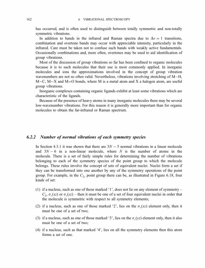
has occurred, and is often used to distinguish between totally symmetric and non-totally
symmetric vibrations.
In addition to bands in the infrared and Raman spectra due to Dv ¼ 1 transitions,
combination and overtone bands may occur with appreciable intensity, particularly in the
infrared. Care must be taken not to confuse such bands with weakly active fundamentals.
Occasionally combinations and, more often, overtones may be used to aid identification of
group vibrations.
Most of the discussion of group vibrations so far has been confined to organic molecules
because it is to such molecules that their use is most commonly applied. In inorganic
molecules and ions the approximations involved in the concept of group vibration
wavenumbers are not so often valid. Nevertheless, vibrations involving stretching of M�H,M�C, M�X and M¼O bonds, where M is a metal atom and X a halogen atom, are useful
group vibrations.
Inorganic complexes containing organic ligands exhibit at least some vibrations which are
characteristic of the ligands.
Because of the presence of heavy atoms in many inorganic molecules there may be several
low-wavenumber vibrations. For this reason it is generally more important than for organic
molecules to obtain the far-infrared or Raman spectrum.
6.2.2 Number of normal vibrations of each symmetry species
In Section 4.3.1 it was shown that there are 3N � 5 normal vibrations in a linear molecule
and 3N � 6 in a non-linear molecule, where N is the number of atoms in the
molecule. There is a set of fairly simple rules for determining the number of vibrations
belonging to each of the symmetry species of the point group to which the molecule
belongs. These rules involve the concept of sets of equivalent nuclei. Nuclei form a set if
they can be transformed into one another by any of the symmetry operations of the point
group. For example, in the C2v point group there can be, as illustrated in Figure 6.18, four
kinds of set:
(1) if a nucleus, such as one of those marked ‘1’, does not lie on any element of symmetry –
C2, svðxzÞ or svðyzÞ – then it must be one of a set of four equivalent nuclei in order that
the molecule is symmetric with respect to all symmetry elements;
(2) if a nucleus, such as one of those marked ‘2’, lies on the svðxzÞ element only, then it
must be one of a set of two;
(3) if a nucleus, such as one of those marked ‘3’, lies on the svðyzÞ element only, then it also
must be one of a set of two;
(4) if a nucleus, such as that marked ‘4’, lies on all the symmetry elements then this atom
forms a set of one.
162 6 VIBRATIONAL SPECTROSCOPY
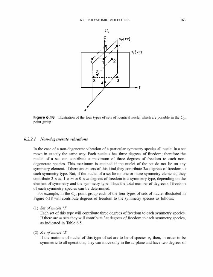
6.2.2.1 Non-degenerate vibrations
In the case of a non-degenerate vibration of a particular symmetry species all nuclei in a set
move in exactly the same way. Each nucleus has three degrees of freedom; therefore the
nuclei of a set can contribute a maximum of three degrees of freedom to each non-
degenerate species. This maximum is attained if the nuclei of the set do not lie on any
symmetry element. If there are m sets of this kind they contribute 3m degrees of freedom to
each symmetry type. But, if the nuclei of a set lie on one or more symmetry elements, they
contribute 2� m, 1� m or 0� m degrees of freedom to a symmetry type, depending on the
element of symmetry and the symmetry type. Thus the total number of degrees of freedom
of each symmetry species can be determined.
For example, in the C2v point group each of the four types of sets of nuclei illustrated in
Figure 6.18 will contribute degrees of freedom to the symmetry species as follows:
(1) Set of nuclei ‘1’
Each set of this type will contribute three degrees of freedom to each symmetry species.
If there are m sets they will contribute 3m degrees of freedom to each symmetry species,
as indicated in Table 6.5.
(2) Set of nuclei ‘2’
If the motions of nuclei of this type of set are to be of species a1 then, in order to be
symmetric to all operations, they can move only in the xz-plane and have two degrees of
Figure 6.18 Illustration of the four types of sets of identical nuclei which are possible in the C2vpoint group
6.2 POLYATOMIC MOLECULES 163
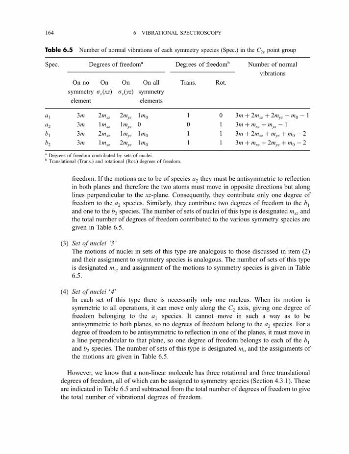
freedom. If the motions are to be of species a2 they must be antisymmetric to reflection
in both planes and therefore the two atoms must move in opposite directions but along
lines perpendicular to the xz-plane. Consequently, they contribute only one degree of
freedom to the a2 species. Similarly, they contribute two degrees of freedom to the b1and one to the b2 species. The number of sets of nuclei of this type is designated mxz and
the total number of degrees of freedom contributed to the various symmetry species are
given in Table 6.5.
(3) Set of nuclei ‘3’
The motions of nuclei in sets of this type are analogous to those discussed in item (2)
and their assignment to symmetry species is analogous. The number of sets of this type
is designated myz and assignment of the motions to symmetry species is given in Table
6.5.
(4) Set of nuclei ‘4’
In each set of this type there is necessarily only one nucleus. When its motion is
symmetric to all operations, it can move only along the C2 axis, giving one degree of
freedom belonging to the a1 species. It cannot move in such a way as to be
antisymmetric to both planes, so no degrees of freedom belong to the a2 species. For a
degree of freedom to be antisymmetric to reflection in one of the planes, it must move in
a line perpendicular to that plane, so one degree of freedom belongs to each of the b1and b2 species. The number of sets of this type is designated mo and the assignments of
the motions are given in Table 6.5.
However, we know that a non-linear molecule has three rotational and three translational
degrees of freedom, all of which can be assigned to symmetry species (Section 4.3.1). These
are indicated in Table 6.5 and subtracted from the total number of degrees of freedom to give
the total number of vibrational degrees of freedom.
Table 6.5 Number of normal vibrations of each symmetry species (Spec.) in the C2v point group
Spec. Degrees of freedoma Degrees of freedomb Number of normal
vibrations
On no
symmetry
element
On
svðxzÞOn
svðyzÞOn all
symmetry
elements
Trans. Rot.
a1 3m 2mxz 2myz 1m0 1 0 3mþ 2mxz þ 2myz þ m0 � 1
a2 3m 1mxz 1myz 0 0 1 3mþ mxz þ myz � 1
b1 3m 2mxz 1myz 1m0 1 1 3mþ 2mxz þ myz þ m0 � 2
b2 3m 1mxz 2myz 1m0 1 1 3mþ mxz þ 2myz þ m0 � 2
a Degrees of freedom contributed by sets of nuclei.b Translational (Trans.) and rotational (Rot.) degrees of freedom.
164 6 VIBRATIONAL SPECTROSCOPY
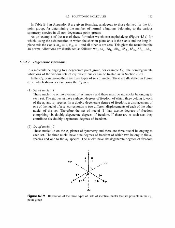
In Table B.1 in Appendix B are given formulae, analogous to those derived for the C2vpoint group, for determining the number of normal vibrations belonging to the various
symmetry species in all non-degenerate point groups.
As an example of the use of these formulae we choose naphthalene (Figure 4.3c) for
which, using the axis notation in which the short in-plane axis is the z axis and the long in-
plane axis the y axis, myz ¼ 4, m2z ¼ 1 and all other m are zero. This gives the result that the
48 normal vibrations are distributed as follows: 9ag, 4au, 3b1g, 8b1u, 4b2g, 8b2u, 8b3g, 4b3u.
6.2.2.2 Degenerate vibrations
In a molecule belonging to a degenerate point group, for example C3v, the non-degenerate
vibrations of the various sets of equivalent nuclei can be treated as in Section 6.2.2.1.
In the C3v point group there are three types of sets of nuclei. These are illustrated in Figure
6.19, which shows a view down the C3 axis.
(1) Set of nuclei ‘1’
These nuclei lie on no element of symmetry and there must be six nuclei belonging to
each set. The six nuclei have eighteen degrees of freedom of which three belong to each
of the a1 and a2 species. In a doubly degenerate degree of freedom, a displacement of
one of the nuclei of a set corresponds to two different displacements of each of the other
nuclei of the set. Therefore the set of nuclei ‘1’ has twelve degrees of freedom
comprising six doubly degenerate degrees of freedom. If there are m such sets they
contribute 6m doubly degenerate degrees of freedom.
(2) Set of nuclei ‘2’
These nuclei lie on the sv planes of symmetry and there are three nuclei belonging to
each set. The three nuclei have nine degrees of freedom of which two belong to the a1species and one to the a2 species. The nuclei have six degenerate degrees of freedom
Figure 6.19 Illustration of the three types of sets of identical nuclei that are possible in the C3vpoint group
6.2 POLYATOMIC MOLECULES 165
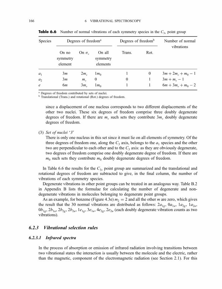
since a displacement of one nucleus corresponds to two different displacements of the
other two nuclei. These six degrees of freedom comprise three doubly degenerate
degrees of freedom. If there are mv such sets they contribute 3mv doubly degenerate
degrees of freedom.
(3) Set of nuclei ‘3’
There is only one nucleus in this set since it must lie on all elements of symmetry. Of the
three degrees of freedom one, along the C3 axis, belongs to the a1 species and the other
two are perpendicular to each other and to the C3 axis: as they are obviously degenerate,
two degrees of freedom comprise one doubly degenerate degree of freedom. If there are
m0 such sets they contribute m0 doubly degenerate degrees of freedom.
In Table 6.6 the results for the C3v point group are summarized and the translational and
rotational degrees of freedom are subtracted to give, in the final column, the number of
vibrations of each symmetry species.
Degenerate vibrations in other point groups can be treated in an analogous way. Table B.2
in Appendix B lists the formulae for calculating the number of degenerate and non-
degenerate vibrations in molecules belonging to degenerate point groups.
As an example, for benzene (Figure 4.3e) m2 ¼ 2 and all the other m are zero, which gives
the result that the 30 normal vibrations are distributed as follows: 2a1g, 0a1u, 1a2g, 1a2u,
0b1g, 2b1u, 2b2g, 2b2u, 1e1g, 3e1u, 4e2g, 2e2u (each doubly degenerate vibration counts as two
vibrations).
6.2.3 Vibrational selection rules
6.2.3.1 Infrared spectra
In the process of absorption or emission of infrared radiation involving transitions between
two vibrational states the interaction is usually between the molecule and the electric, rather
than the magnetic, component of the electromagnetic radiation (see Section 2.1). For this
Table 6.6 Number of normal vibrations of each symmetry species in the C3v point group
Species Degrees of freedoma Degrees of freedomb Number of normal
vibrations
On no
symmetry
element
On sv On all
symmetry
elements
Trans. Rot.
a1 3m 2mv 1m0 1 0 3mþ 2mv þ m0 � 1
a2 3m mv 0 0 1 3mþ mv � 1
e 6m 3mv 1m0 1 1 6mþ 3mv þ m0 � 2
a Degrees of freedom contributed by sets of nuclei.b Translational (Trans.) and rotational (Rot.) degrees of freedom.
166 6 VIBRATIONAL SPECTROSCOPY
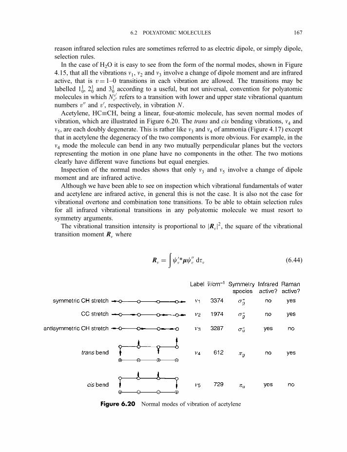
reason infrared selection rules are sometimes referred to as electric dipole, or simply dipole,
selection rules.
In the case of H2O it is easy to see from the form of the normal modes, shown in Figure
4.15, that all the vibrations n1, n2 and n3 involve a change of dipole moment and are infrared
active, that is v¼ 1–0 transitions in each vibration are allowed. The transitions may be
labelled 110, 210 and 310 according to a useful, but not universal, convention for polyatomic
molecules in which N v0v00 refers to a transition with lower and upper state vibrational quantum
numbers v00 and v0, respectively, in vibration N .
Acetylene, HCCH, being a linear, four-atomic molecule, has seven normal modes of
vibration, which are illustrated in Figure 6.20. The trans and cis bending vibrations, n4 andn5, are each doubly degenerate. This is rather like n3 and n4 of ammonia (Figure 4.17) except
that in acetylene the degeneracy of the two components is more obvious. For example, in the
n4 mode the molecule can bend in any two mutually perpendicular planes but the vectors
representing the motion in one plane have no components in the other. The two motions
clearly have different wave functions but equal energies.
Inspection of the normal modes shows that only n3 and n5 involve a change of dipole
moment and are infrared active.
Although we have been able to see on inspection which vibrational fundamentals of water
and acetylene are infrared active, in general this is not the case. It is also not the case for
vibrational overtone and combination tone transitions. To be able to obtain selection rules
for all infrared vibrational transitions in any polyatomic molecule we must resort to
symmetry arguments.
The vibrational transition intensity is proportional to jRvj2, the square of the vibrational
transition moment Rv where
Rv ¼ðcv0*mmc00v dtv ð6:44Þ
Figure 6.20 Normal modes of vibration of acetylene
6.2 POLYATOMIC MOLECULES 167
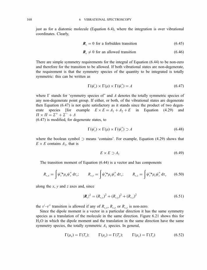
just as for a diatomic molecule (Equation 6.4), where the integration is over vibrational
coordinates. Clearly,
Rv ¼ 0 for a forbidden transition ð6:45ÞRv 6¼ 0 for an allowed transition ð6:46Þ
There are simple symmetry requirements for the integral of Equation (6.44) to be non-zero
and therefore for the transition to be allowed. If both vibrational states are non-degenerate,
the requirement is that the symmetry species of the quantity to be integrated is totally
symmetric: this can be written as
Gðc0vÞ � GðmÞ � Gðc00v Þ ¼ A ð6:47Þ
where G stands for ‘symmetry species of’ and A denotes the totally symmetric species of
any non-degenerate point group. If either, or both, of the vibrational states are degenerate
then Equation (6.47) is not quite satisfactory as it stands since the product of two degen-
erate species [for example E � E ¼ A1 þ A2 þ E in Equation (4.29) and
P�P ¼ Sþ þ S� þ D in Equation (4.33)] results in more than one species. So Equation
(6.47) is modified, for degenerate states, to
Gðc0vÞ � GðmÞ � Gðc00v Þ � A ð6:48Þ
where the boolean symbol � means ‘contains’. For example, Equation (4.29) shows that
E � E contains A1, that is
E � E � A1 ð6:49Þ
The transition moment of Equation (6.44) is a vector and has components
Rv;x ¼ðcv0*mxc
00v dtv; Rv;y ¼
ðcv0*myc
00v dtv; Rv;z ¼
ðcv0*mzc
00v dtv ð6:50Þ
along the x, y and z axes and, since
jRvj2 ¼ ðRv;xÞ2 þ ðRv;yÞ2 þ ðRv;zÞ2 ð6:51Þ
the v0–v00 transition is allowed if any of Rv;x, Rv;y or Rv;z is non-zero.
Since the dipole moment is a vector in a particular direction it has the same symmetry
species as a translation of the molecule in the same direction. Figure 6.21 shows this for
H2O in which the dipole moment and the translation in the same direction have the same
symmetry species, the totally symmetric A1 species. In general,
GðmxÞ ¼ GðTxÞ; GðmyÞ ¼ GðTyÞ; GðmzÞ ¼ GðTzÞ ð6:52Þ
168 6 VIBRATIONAL SPECTROSCOPY
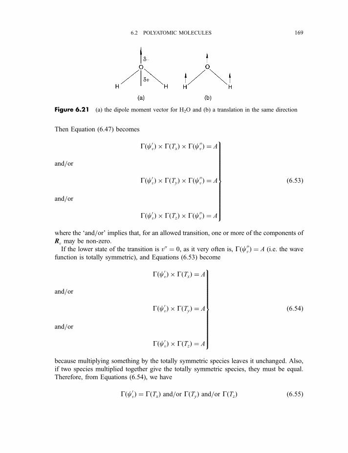
Then Equation (6.47) becomes
Gðc0vÞ � GðTxÞ � Gðc00v Þ ¼ A
and=or
Gðc0vÞ � GðTyÞ � Gðc00v Þ ¼ A ð6:53Þ
and=or
Gðc0vÞ � GðTzÞ � Gðc00v Þ ¼ A
where the ‘and=or’ implies that, for an allowed transition, one or more of the components of
Rv may be non-zero.
If the lower state of the transition is v00 ¼ 0, as it very often is, Gðc00v Þ ¼ A (i.e. the wave
function is totally symmetric), and Equations (6.53) become
Gðc0vÞ � GðTxÞ ¼ A
and=or
Gðc0vÞ � GðTyÞ ¼ A ð6:54Þ
and=or
Gðc0vÞ � GðTzÞ ¼ A
because multiplying something by the totally symmetric species leaves it unchanged. Also,
if two species multiplied together give the totally symmetric species, they must be equal.
Therefore, from Equations (6.54), we have
Gðc0vÞ ¼ GðTxÞ and=or GðTyÞ and=or GðTzÞ ð6:55Þ
Figure 6.21 (a) the dipole moment vector for H2O and (b) a translation in the same direction
9>>>>>>>>>>>>>>=>>>>>>>>>>>>>>;
9>>>>>>>>>>>>>>=>>>>>>>>>>>>>>;
6.2 POLYATOMIC MOLECULES 169
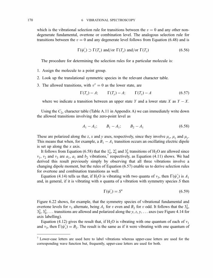
which is the vibrational selection rule for transitions between the v ¼ 0 and any other non-
degenerate fundamental, overtone or combination level. The analogous selection rule for
transitions between the v ¼ 0 and any degenerate level follows from Equation (6.48) and is
Gðc0vÞ � GðTxÞ and=or GðTyÞ and=or GðTzÞ ð6:56Þ
The procedure for determining the selection rules for a particular molecule is:
1. Assign the molecule to a point group.
2. Look up the translational symmetric species in the relevant character table.
3. The allowed transitions, with v00 ¼ 0 as the lower state, are
GðTxÞ � A; GðTyÞ � A; GðTzÞ � A ð6:57Þwhere we indicate a transition between an upper state Y and a lower state X as Y � X .
Using the C2v character table (Table A.11 in Appendix A) we can immediately write down
the allowed transitions involving the zero-point level as
A1 � A1; B1 � A1; B2 � A1 ð6:58Þ
These are polarized along the z, x and y axes, respectively, since they involve mz, mx and my.This means that when, for example, a B1 � A1 transition occurs an oscillating electric dipole
is set up along the x axis.
It follows from Equation (6.58) that the 110, 210 and 310 transitions of H2O are allowed since
n1, n2 and n3 are a1, a1 and b2 vibrations,7 respectively, as Equation (4.11) shows. We had
derived this result previously simply by observing that all three vibrations involve a
changing dipole moment, but the rules of Equation (6.57) enable us to derive selection rules
for overtone and combination transitions as well.
Equation (4.14) tells us that, if H2O is vibrating with two quanta of n3, then Gðc0vÞ is A1
and, in general, if it is vibrating with n quanta of a vibration with symmetry species S then
Gðc0vÞ ¼ Sn ð6:59Þ
Figure 6.22 shows, for example, that the symmetry species of vibrational fundamental and
overtone levels for n3 alternate, being A1 for v even and B2 for v odd. It follows that the 310,320, 3
30; . . . transitions are allowed and polarized along the y, z, y; . . . axes (see Figure 4.14 for
axis labelling).
Equation (4.12) gives the result that, if H2O is vibrating with one quantum of each of n1and n3, then Gðc0vÞ ¼ B2. The result is the same as if it were vibrating with one quantum of
7 Lower-case letters are used here to label vibrations whereas upper-case letters are used for the
corresponding wave function but, frequently, upper-case letters are used for both.
170 6 VIBRATIONAL SPECTROSCOPY
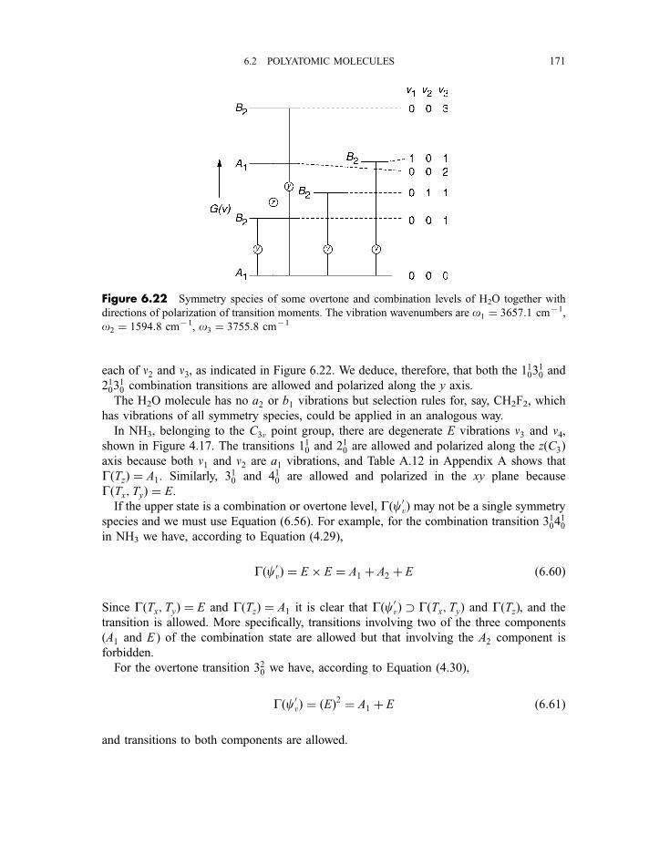
each of n2 and n3, as indicated in Figure 6.22. We deduce, therefore, that both the 110310 and
210310 combination transitions are allowed and polarized along the y axis.
The H2O molecule has no a2 or b1 vibrations but selection rules for, say, CH2F2, which
has vibrations of all symmetry species, could be applied in an analogous way.
In NH3, belonging to the C3v point group, there are degenerate E vibrations n3 and n4,shown in Figure 4.17. The transitions 110 and 210 are allowed and polarized along the zðC3Þaxis because both n1 and n2 are a1 vibrations, and Table A.12 in Appendix A shows that
GðTzÞ ¼ A1. Similarly, 310 and 410 are allowed and polarized in the xy plane because
GðTx; TyÞ ¼ E.
If the upper state is a combination or overtone level, Gðc0vÞ may not be a single symmetry
species and we must use Equation (6.56). For example, for the combination transition 310410
in NH3 we have, according to Equation (4.29),
Gðc0vÞ ¼ E � E ¼ A1 þ A2 þ E ð6:60Þ
Since GðTx; TyÞ ¼ E and GðTzÞ ¼ A1 it is clear that Gðc0vÞ � GðTx; TyÞ and GðTzÞ, and the
transition is allowed. More specifically, transitions involving two of the three components
(A1 and E ) of the combination state are allowed but that involving the A2 component is
forbidden.
For the overtone transition 320 we have, according to Equation (4.30),
Gðc0vÞ ¼ ðEÞ2 ¼ A1 þ E ð6:61Þ
and transitions to both components are allowed.
Figure 6.22 Symmetry species of some overtone and combination levels of H2O together with
directions of polarization of transition moments. The vibration wavenumbers are o1 ¼ 3657:1 cm71,
o2 ¼ 1594:8 cm71, o3 ¼ 3755:8 cm71
6.2 POLYATOMIC MOLECULES 171
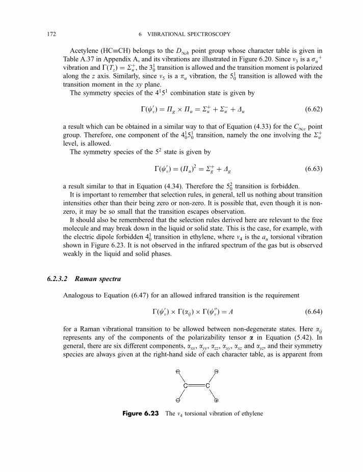
Acetylene (HCCH) belongs to the D1h point group whose character table is given in
Table A.37 in Appendix A, and its vibrations are illustrated in Figure 6.20. Since n3 is a suþ
vibration and GðTzÞ ¼ Sþu , the 310 transition is allowed and the transition moment is polarized
along the z axis. Similarly, since n5 is a pu vibration, the 510 transition is allowed with the
transition moment in the xy plane.
The symmetry species of the 4151 combination state is given by
Gðc0vÞ ¼ Pg �Pu ¼ Sþu þ S�u þ Du ð6:62Þ
a result which can be obtained in a similar way to that of Equation (4.33) for the C1v point
group. Therefore, one component of the 410510 transition, namely the one involving the Sþu
level, is allowed.
The symmetry species of the 52 state is given by
Gðc0vÞ ¼ ðPuÞ2 ¼ Sþg þ Dg ð6:63Þ
a result similar to that in Equation (4.34). Therefore the 520 transition is forbidden.
It is important to remember that selection rules, in general, tell us nothing about transition
intensities other than their being zero or non-zero. It is possible that, even though it is non-
zero, it may be so small that the transition escapes observation.
It should also be remembered that the selection rules derived here are relevant to the free
molecule and may break down in the liquid or solid state. This is the case, for example, with
the electric dipole forbidden 410 transition in ethylene, where n4 is the au torsional vibrationshown in Figure 6.23. It is not observed in the infrared spectrum of the gas but is observed
weakly in the liquid and solid phases.
6.2.3.2 Raman spectra
Analogous to Equation (6.47) for an allowed infrared transition is the requirement
Gðc0vÞ � GðaijÞ � Gðc00v Þ ¼ A ð6:64Þ
for a Raman vibrational transition to be allowed between non-degenerate states. Here aijrepresents any of the components of the polarizability tensor aa in Equation (5.42). In
general, there are six different components, axx, ayy, azz, axy, axz and ayz, and their symmetry
species are always given at the right-hand side of each character table, as is apparent from
Figure 6.23 The n4 torsional vibration of ethylene
172 6 VIBRATIONAL SPECTROSCOPY
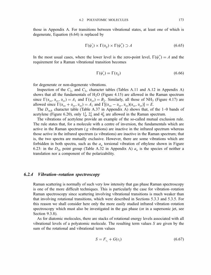
those in Appendix A. For transitions between vibrational states, at least one of which is
degenerate, Equation (6.64) is replaced by
Gðc0vÞ � GðaijÞ � Gðc00v Þ � A ð6:65Þ
In the most usual cases, where the lower level is the zero-point level, Gðc00v Þ ¼ A and the
requirement for a Raman vibrational transition becomes
Gðc0vÞ ¼ GðaijÞ ð6:66Þ
for degenerate or non-degenerate vibrations.
Inspection of the C2v and C3v character tables (Tables A.11 and A.12 in Appendix A)
shows that all the fundamentals of H2O (Figure 4.15) are allowed in the Raman spectrum
since Gðaxx; ayy; azzÞ ¼ A1 and GðayzÞ ¼ B2. Similarly, all those of NH3 (Figure 4.17) are
allowed since Gðaxx þ ayy; azzÞ ¼ A1 and G½ðaxx � ayy; axyÞðaxz; ayzÞ� ¼ E.
The D1h character table (Table A.37 in Appendix A) shows that, of the 1–0 bands of
acetylene (Figure 6.20), only 110, 210 and 410 are allowed in the Raman spectrum.
The vibrations of acetylene provide an example of the so-called mutual exclusion rule.
The rule states that, for a molecule with a centre of inversion, the fundamentals which are
active in the Raman spectrum (g vibrations) are inactive in the infrared spectrum whereas
those active in the infrared spectrum (u vibrations) are inactive in the Raman spectrum; that
is, the two spectra are mutually exclusive. However, there are some vibrations which are
forbidden in both spectra, such as the au torsional vibration of ethylene shown in Figure
6.23: in the D2h point group (Table A.32 in Appendix A) au is the species of neither a
translation nor a component of the polarizability.
6.2.4 Vibration–rotation spectroscopy
Raman scattering is normally of such very low intensity that gas phase Raman spectroscopy
is one of the more difficult techniques. This is particularly the case for vibration–rotation
Raman spectroscopy since scattering involving vibrational transitions is much weaker than
that involving rotational transitions, which were described in Sections 5.3.3 and 5.3.5. For
this reason we shall consider here only the more easily studied infrared vibration–rotation
spectroscopy which must also be investigated in the gas phase (or in a supersonic jet, see
Section 9.3.8).
As for diatomic molecules, there are stacks of rotational energy levels associated with all
vibrational levels of a polyatomic molecule. The resulting term values S are given by the
sum of the rotational and vibrational term values
S ¼ Fvi þ GðviÞ ð6:67Þ
6.2 POLYATOMIC MOLECULES 173
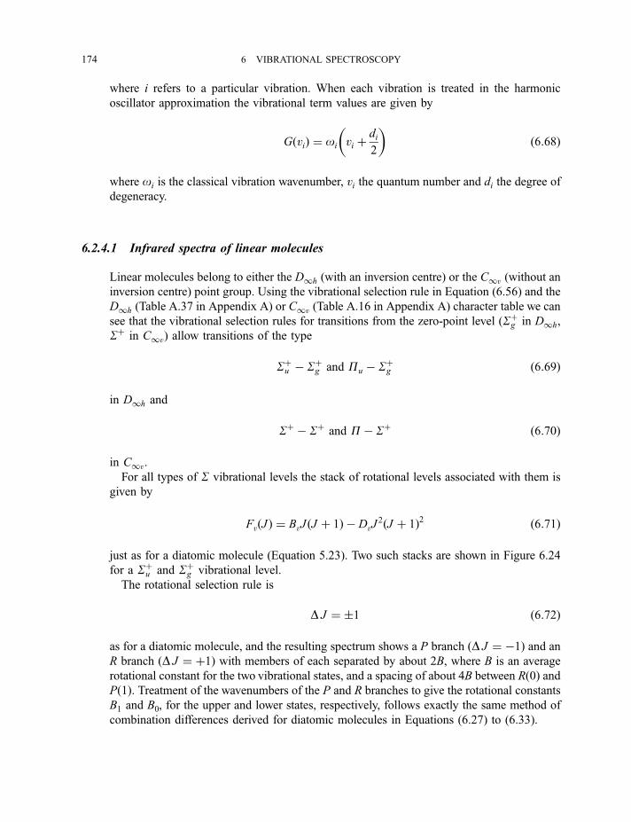
where i refers to a particular vibration. When each vibration is treated in the harmonic
oscillator approximation the vibrational term values are given by
GðviÞ ¼ oi vi þdi
2
� �ð6:68Þ
where oi is the classical vibration wavenumber, vi the quantum number and di the degree of
degeneracy.
6.2.4.1 Infrared spectra of linear molecules
Linear molecules belong to either the D1h (with an inversion centre) or the C1v (without an
inversion centre) point group. Using the vibrational selection rule in Equation (6.56) and the
D1h (Table A.37 in Appendix A) or C1v (Table A.16 in Appendix A) character table we can
see that the vibrational selection rules for transitions from the zero-point level (Sþg in D1h,
Sþ in C1v) allow transitions of the type
Sþu � Sþg and Pu � Sþg ð6:69Þ
in D1h and
Sþ � Sþ and P� Sþ ð6:70Þ
in C1v.
For all types of S vibrational levels the stack of rotational levels associated with them is
given by
FvðJ Þ ¼ BvJ ðJ þ 1Þ � DvJ2ðJ þ 1Þ2 ð6:71Þ
just as for a diatomic molecule (Equation 5.23). Two such stacks are shown in Figure 6.24
for a Sþu and Sþg vibrational level.
The rotational selection rule is
D J ¼ �1 ð6:72Þ
as for a diatomic molecule, and the resulting spectrum shows a P branch ðD J ¼ �1Þ and an
R branch ðD J ¼ þ1Þ with members of each separated by about 2B, where B is an average
rotational constant for the two vibrational states, and a spacing of about 4B between Rð0Þ andPð1Þ. Treatment of the wavenumbers of the P and R branches to give the rotational constants
B1 and B0, for the upper and lower states, respectively, follows exactly the same method of
combination differences derived for diatomic molecules in Equations (6.27) to (6.33).
174 6 VIBRATIONAL SPECTROSCOPY
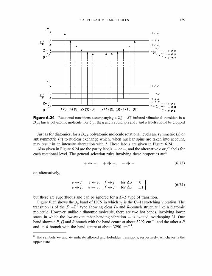
Just as for diatomics, for a D1h polyatomic molecule rotational levels are symmetric ðsÞ orantisymmetric ðaÞ to nuclear exchange which, when nuclear spins are taken into account,
may result in an intensity alternation with J . These labels are given in Figure 6.24.
Also given in Figure 6.24 are the parity labels, þ or �, and the alternative e or f labels foreach rotational level. The general selection rules involving these properties are8
þ $ �; þ $j þ; � $j � ð6:73Þ
or, alternatively,
e$ f ; e$j e; f $j f for D J ¼ 0
e$j f ; e$ e; f $ f for D J ¼ �1�
ð6:74Þ
but these are superfluous and can be ignored for a S–S type of transition.
Figure 6.25 shows the 310 band of HCN in which n3 is the C�H stretching vibration. The
transition is of the Sþ–Sþ type showing clear P- and R-branch structure like a diatomic
molecule. However, unlike a diatomic molecule, there are two hot bands, involving lower
states in which the low-wavenumber bending vibration n2 is excited, overlapping 310. One
band shows a P, Q and R branch with the band centre at about 3292 cm71 and the other a P
and an R branch with the band centre at about 3290 cm71.
Figure 6.24 Rotational transitions accompanying a Sþu � Sþg infrared vibrational transition in a
D1h linear polyatomic molecule. For C1v the g and u subscripts and s and a labels should be dropped
8 The symbols $ and $j indicate allowed and forbidden transitions, respectively, whichever is the
upper state.
6.2 POLYATOMIC MOLECULES 175
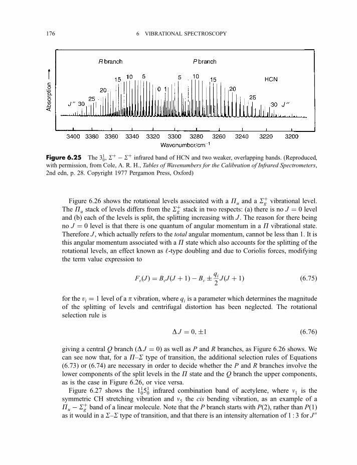
Figure 6.26 shows the rotational levels associated with a Pu and a Sþg vibrational level.
The Pu stack of levels differs from the Sþg stack in two respects: (a) there is no J ¼ 0 level
and (b) each of the levels is split, the splitting increasing with J . The reason for there being
no J ¼ 0 level is that there is one quantum of angular momentum in a P vibrational state.
Therefore J , which actually refers to the total angular momentum, cannot be less than 1. It is
this angular momentum associated with aP state which also accounts for the splitting of the
rotational levels, an effect known as ‘-type doubling and due to Coriolis forces, modifying
the term value expression to
FvðJ Þ ¼ BvJ ðJ þ 1Þ � Bv �qi
2J ðJ þ 1Þ ð6:75Þ
for the vi ¼ 1 level of a p vibration, where qi is a parameter which determines the magnitude
of the splitting of levels and centrifugal distortion has been neglected. The rotational
selection rule is
D J ¼ 0;�1 ð6:76Þ
giving a central Q branch ðD J ¼ 0Þ as well as P and R branches, as Figure 6.26 shows. We
can see now that, for a P–S type of transition, the additional selection rules of Equations
(6.73) or (6.74) are necessary in order to decide whether the P and R branches involve the
lower components of the split levels in the P state and the Q branch the upper components,
as is the case in Figure 6.26, or vice versa.
Figure 6.27 shows the 110510 infrared combination band of acetylene, where n1 is the
symmetric CH stretching vibration and n5 the cis bending vibration, as an example of a
Pu � Sþg band of a linear molecule. Note that the P branch starts with Pð2Þ, rather than Pð1Þas it would in a S–S type of transition, and that there is an intensity alternation of 1 : 3 for J 00
Figure 6.25 The 310, Sþ � Sþ infrared band of HCN and two weaker, overlapping bands. (Reproduced,
with permission, from Cole, A. R. H., Tables of Wavenumbers for the Calibration of Infrared Spectrometers,
2nd edn, p. 28. Copyright 1977 Pergamon Press, Oxford)
176 6 VIBRATIONAL SPECTROSCOPY
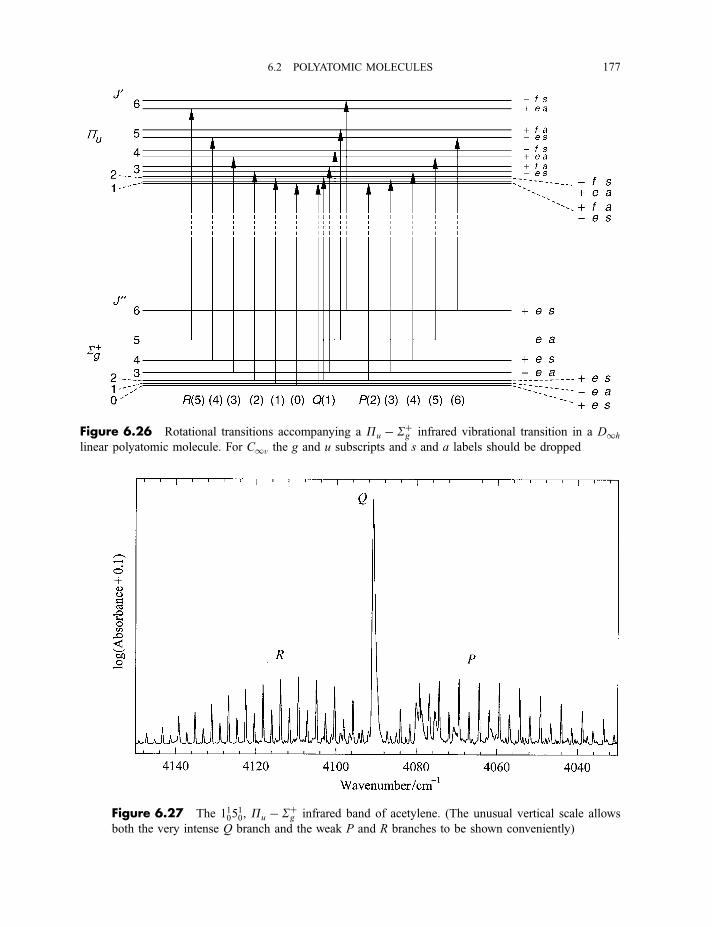
Figure 6.27 The 110510, Pu � Sþg infrared band of acetylene. (The unusual vertical scale allows
both the very intense Q branch and the weak P and R branches to be shown conveniently)
Figure 6.26 Rotational transitions accompanying a Pu � Sþg infrared vibrational transition in a D1h
linear polyatomic molecule. For C1v the g and u subscripts and s and a labels should be dropped
6.2 POLYATOMIC MOLECULES 177
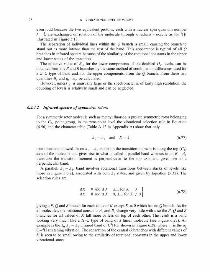
even : odd because the two equivalent protons, each with a nuclear spin quantum number
I ¼ 12, are exchanged on rotation of the molecule through p radians – exactly as for 1H2
illustrated in Figure 5.18.
The separation of individual lines within the Q branch is small, causing the branch to
stand out as more intense than the rest of the band. This appearance is typical of all Q
branches in infrared spectra because of the similarity of the rotational constants in the upper
and lower states of the transition.
The effective value of Bv, for the lower components of the doubled Pu levels, can be
obtained from the P and R branches by the same method of combination differences used for
a S–S type of band and, for the upper components, from the Q branch. From these two
quantities Bv and qi may be calculated.
However, unless qi is unusually large or the spectrometer is of fairly high resolution, the
doubling of levels is relatively small and can be neglected.
6.2.4.2 Infrared spectra of symmetric rotors
For a symmetric rotor molecule such as methyl fluoride, a prolate symmetric rotor belonging
to the C3v point group, in the zero-point level the vibrational selection rule in Equation
(6.56) and the character table (Table A.12 in Appendix A) show that only
A1 � A1 and E � A1 ð6:77Þ
transitions are allowed. In an A1 � A1 transition the transition moment is along the top ðC3Þaxis of the molecule and gives rise to what is called a parallel band whereas in an E � A1
transition the transition moment is perpendicular to the top axis and gives rise to a
perpendicular band.
A parallel, A1 � A1, band involves rotational transitions between stacks of levels like
those in Figure 5.6(a), associated with both A1 states, and given by Equation (5.32). The
selection rules are
DK ¼ 0 and D J ¼ �1; for K ¼ 0
DK ¼ 0 and D J ¼ 0;�1; for K 6¼ 0
�ð6:78Þ
giving a P, Q and R branch for each value of K except K ¼ 0 which has no Q branch. As for
all molecules, the rotational constants Av and Bv change very little with v so the P, Q and R
branches for all values of K fall more or less on top of each other. The result is a band
looking very much like a P–S type of band of a linear molecule (see Figure 6.27). An
example is the 110 A1 � A1 infrared band of C2H3F, shown in Figure 6.28, where n1 is the a1C�2H stretching vibration. The separation of the central Q branches with different values of
K is seen to be small owing to the similarity of rotational constants in the upper and lower
vibrational states.
178 6 VIBRATIONAL SPECTROSCOPY
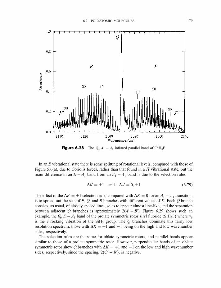
In an E vibrational state there is some splitting of rotational levels, compared with those of
Figure 5.6(a), due to Coriolis forces, rather than that found in a P vibrational state, but the
main difference in an E � A1 band from an A1 � A1 band is due to the selection rules
DK ¼ �1 and D J ¼ 0;�1 ð6:79Þ
The effect of the DK ¼ �1 selection rule, compared with DK ¼ 0 for an A1 � A1 transition,
is to spread out the sets of P, Q, and R branches with different values of K. Each Q branch
consists, as usual, of closely spaced lines, so as to appear almost line-like, and the separation
between adjacent Q branches is approximately 2ðA0 � B0Þ. Figure 6.29 shows such an
example, the 610 E � A1 band of the prolate symmetric rotor silyl fluoride (SiH3F) where n6is the e rocking vibration of the SiH3 group. The Q branches dominate this fairly low
resolution spectrum, those with DK ¼ þ1 and �1 being on the high and low wavenumber
sides, respectively.
The selection rules are the same for oblate symmetric rotors, and parallel bands appear
similar to those of a prolate symmetric rotor. However, perpendicular bands of an oblate
symmetric rotor show Q branches with DK ¼ þ1 and �1 on the low and high wavenumber
sides, respectively, since the spacing, 2ðC0 � B0Þ, is negative.
Figure 6.28 The 110, A1 � A1 infrared parallel band of C2H3F.
6.2 POLYATOMIC MOLECULES 179
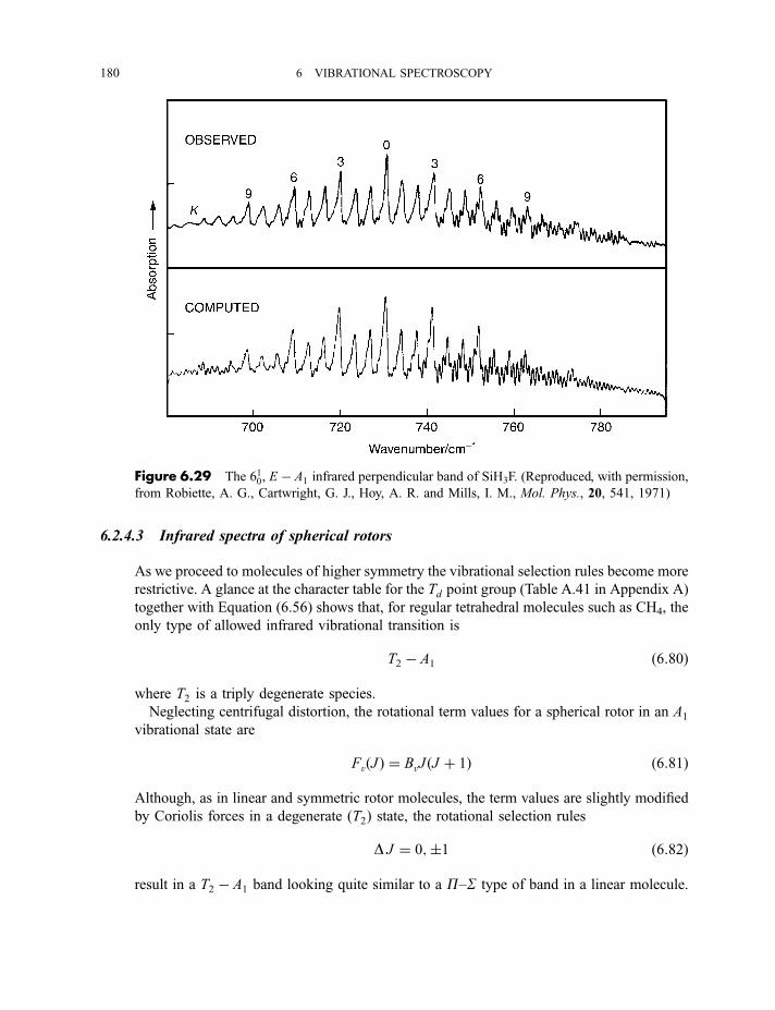
6.2.4.3 Infrared spectra of spherical rotors
As we proceed to molecules of higher symmetry the vibrational selection rules become more
restrictive. A glance at the character table for the Td point group (Table A.41 in Appendix A)
together with Equation (6.56) shows that, for regular tetrahedral molecules such as CH4, the
only type of allowed infrared vibrational transition is
T2 � A1 ð6:80Þ
where T2 is a triply degenerate species.
Neglecting centrifugal distortion, the rotational term values for a spherical rotor in an A1
vibrational state are
FvðJ Þ ¼ BvJ ðJ þ 1Þ ð6:81Þ
Although, as in linear and symmetric rotor molecules, the term values are slightly modified
by Coriolis forces in a degenerate ðT2Þ state, the rotational selection rules
D J ¼ 0;�1 ð6:82Þ
result in a T2 � A1 band looking quite similar to a P–S type of band in a linear molecule.
Figure 6.29 The 610, E � A1 infrared perpendicular band of SiH3F. (Reproduced, with permission,
from Robiette, A. G., Cartwright, G. J., Hoy, A. R. and Mills, I. M., Mol. Phys., 20, 541, 1971)
180 6 VIBRATIONAL SPECTROSCOPY
For a spherical rotor belonging to the octahedral Oh point group, Table A.43 in
Appendix A, in conjunction with the vibrational selection rules of Equation (6.56), show
that the only allowed transitions are
T1u � A1g ð6:83Þ
Such bands also obey the rotational selection rules in Equation (6.82) and appear similar to a
P–S band of a linear molecule.
6.2.4.4 Infrared spectra of asymmetric rotors
As in Section 5.2.4 on rotational spectra of asymmetric rotors, we do not treat this important
group of molecules in any detail, so far as their rotational motion is concerned, because of
the great complexity of their rotational energy levels. Nevertheless, however complex the
stack associated with the v¼ 0 level, there is a very similar stack associated with each
excited vibrational level. The selection rules for transitions between the rotational stacks of
the vibrational levels are also complex but include
D J ¼ 0;�1 ð6:84Þ
giving what may be rather randomly distributed sets of P, Q and R branches.
In a molecule such as the asymmetric rotor formaldehyde, shown in Figure 5.1(f ), the a, b
and c inertial axes, of lowest, medium and highest moments of inertia, respectively, are
defined by symmetry, the a axis being the C2 axis, the b axis being in the yz plane and the c
axis being perpendicular to the yz plane. Vibrational transition moments are confined to the
a, b or c axis and the rotational selection rules are characteristic. We call them
type A; type B; or type C ð6:85Þ
selection rules corresponding to a transition moment along the a, b or c axis respectively.
Whether the molecule is a prolate or an oblate asymmetric rotor, type A, B or C selection
rules result in characteristic band shapes. These shapes, or contours, are particularly
important in gas-phase infrared spectra of large asymmetric rotors, whose rotational lines are
not resolved, for assigning symmetry species to observed fundamentals.
Ethylene (H2C¼CH2) is a prolate asymmetric rotor which is sufficiently small for some
rotational structure to be resolved even when only a medium resolution spectrometer is used.
Figures 6.30, 6.31 and 6.32 show the 1110 (type A), 910 (type B) and 710 (type C) bands of
ethylene, respectively, and Figure 6.33 shows the form and symmetry species of the
vibrations involved. Without looking at the detail we can see that the type A band is
dominated by a strong central peak and fairly weak wings, the type B band by a central
minimum and moderately strong wings, and the type C band by a strong central peak and
moderately strong wings.
6.2 POLYATOMIC MOLECULES 181
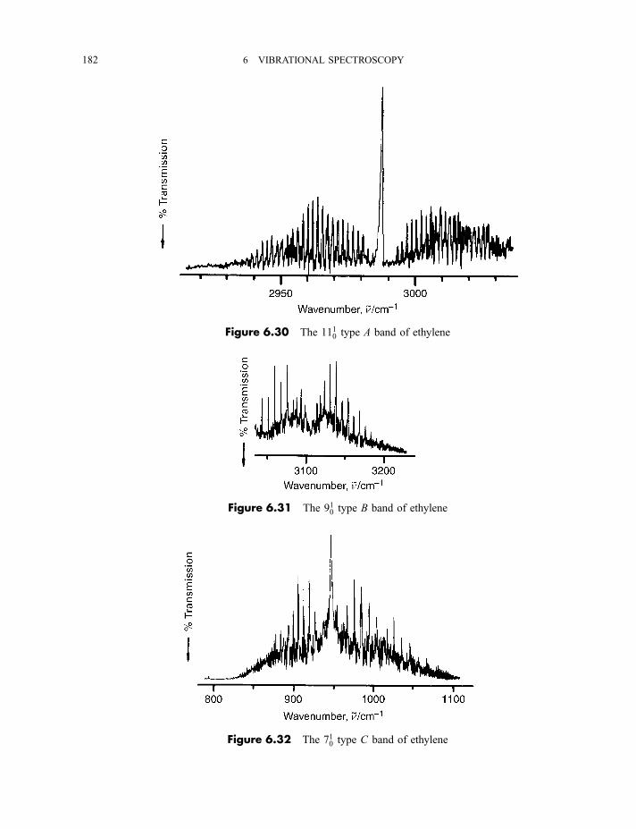
Figure 6.30 The 1110 type A band of ethylene
Figure 6.31 The 910 type B band of ethylene
Figure 6.32 The 710 type C band of ethylene
182 6 VIBRATIONAL SPECTROSCOPY
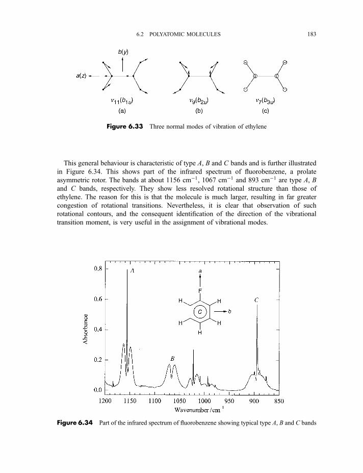
This general behaviour is characteristic of type A, B and C bands and is further illustrated
in Figure 6.34. This shows part of the infrared spectrum of fluorobenzene, a prolate
asymmetric rotor. The bands at about 1156 cm�1, 1067 cm�1 and 893 cm�1 are type A, B
and C bands, respectively. They show less resolved rotational structure than those of
ethylene. The reason for this is that the molecule is much larger, resulting in far greater
congestion of rotational transitions. Nevertheless, it is clear that observation of such
rotational contours, and the consequent identification of the direction of the vibrational
transition moment, is very useful in the assignment of vibrational modes.
Figure 6.33 Three normal modes of vibration of ethylene
Figure 6.34 Part of the infrared spectrum of fluorobenzene showing typical type A, B and C bands
6.2 POLYATOMIC MOLECULES 183
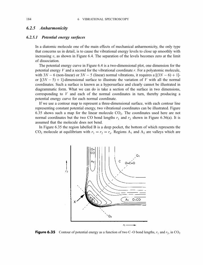
6.2.5 Anharmonicity
6.2.5.1 Potential energy surfaces
In a diatomic molecule one of the main effects of mechanical anharmonicity, the only type
that concerns us in detail, is to cause the vibrational energy levels to close up smoothly with
increasing v, as shown in Figure 6.4. The separation of the levels becomes zero at the limit
of dissociation.
The potential energy curve in Figure 6.4 is a two-dimensional plot, one dimension for the
potential energy V and a second for the vibrational coordinate r. For a polyatomic molecule,
with 3N � 6 (non-linear) or 3N � 5 (linear) normal vibrations, it requires a ½ð3N � 6Þ þ 1�-or ½ð3N � 5Þ þ 1�-dimensional surface to illustrate the variation of V with all the normal
coordinates. Such a surface is known as a hypersurface and clearly cannot be illustrated in
diagrammatic form. What we can do is take a section of the surface in two dimensions,
corresponding to V and each of the normal coordinates in turn, thereby producing a
potential energy curve for each normal coordinate.
If we use a contour map to represent a three-dimensional surface, with each contour line
representing constant potential energy, two vibrational coordinates can be illustrated. Figure
6.35 shows such a map for the linear molecule CO2. The coordinates used here are not
normal coordinates but the two CO bond lengths r1 and r2 shown in Figure 6.36(a). It is
assumed that the molecule does not bend.
In Figure 6.35 the region labelled B is a deep pocket, the bottom of which represents the
CO2 molecule at equilibrium with r1 ¼ r2 ¼ re. Regions A1 and A2 are valleys which are
Figure 6.35 Contour of potential energy as a function of two C–O bond lengths, r1 and r2, in CO2
184 6 VIBRATIONAL SPECTROSCOPY
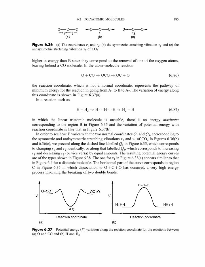
higher in energy than B since they correspond to the removal of one of the oxygen atoms,
leaving behind a CO molecule. In the atom–molecule reaction
Oþ CO! OCO! OCþ O ð6:86Þ
the reaction coordinate, which is not a normal coordinate, represents the pathway of
minimum energy for the reaction in going from A1 to B to A2. The variation of energy along
this coordinate is shown in Figure 6.37(a).
In a reaction such as
Hþ H2! H � � �H � � �H! H2 þ H ð6:87Þ
in which the linear triatomic molecule is unstable, there is an energy maximum
corresponding to the region B in Figure 6.35 and the variation of potential energy with
reaction coordinate is like that in Figure 6.37(b).
In order to see how V varies with the two normal coordinates Q1 and Q3, corresponding to
the symmetric and antisymmetric stretching vibrations n1 and n3 of CO2 in Figures 6.36(b)
and 6.36(c), we proceed along the dashed line labelled Q1 in Figure 6.35, which corresponds
to changing r1 and r2 identically, or along that labelled Q3, which corresponds to increasing
r1 and decreasing r2 (or vice versa) by equal amounts. The resulting potential energy curves
are of the types shown in Figure 6.38. The one for n1 in Figure 6.38(a) appears similar to that
in Figure 6.4 for a diatomic molecule. The horizontal part of the curve corresponds to region
C in Figure 6.35 in which dissociation to OþCþO has occurred, a very high energy
process involving the breaking of two double bonds.
Figure 6.37 Potential energy ðV Þ variation along the reaction coordinate for the reactions between
(a) O and CO and (b) H and H2
Figure 6.36 (a) The coordinates r1 and r2, (b) the symmetric stretching vibration n1 and (c) the
antisymmetric stretching vibration n3 of CO2
6.2 POLYATOMIC MOLECULES 185
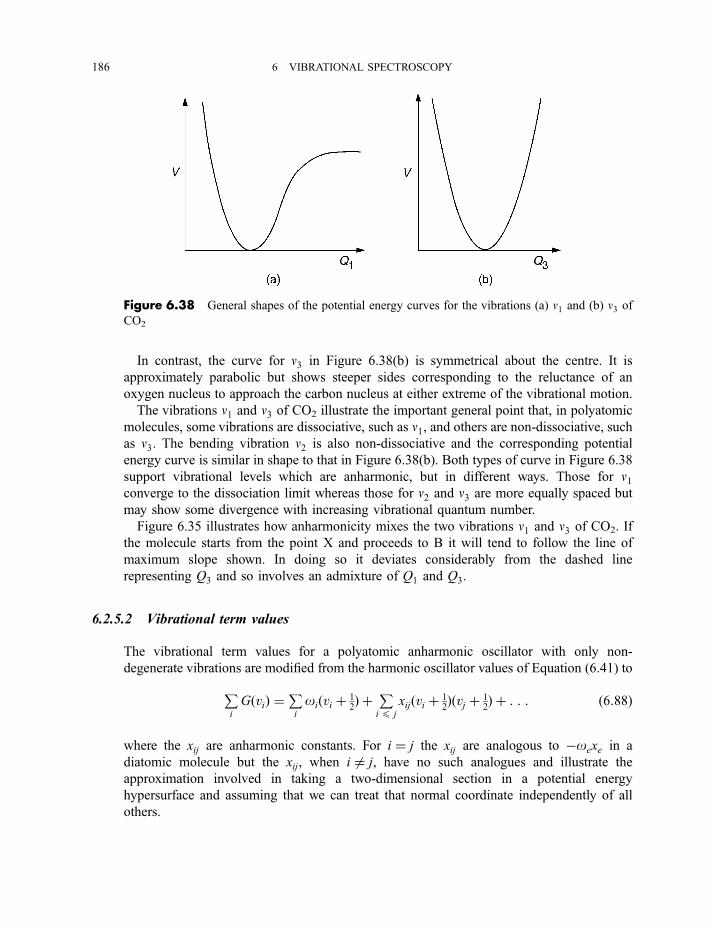
In contrast, the curve for n3 in Figure 6.38(b) is symmetrical about the centre. It is
approximately parabolic but shows steeper sides corresponding to the reluctance of an
oxygen nucleus to approach the carbon nucleus at either extreme of the vibrational motion.
The vibrations n1 and n3 of CO2 illustrate the important general point that, in polyatomic
molecules, some vibrations are dissociative, such as n1, and others are non-dissociative, suchas n3. The bending vibration n2 is also non-dissociative and the corresponding potential
energy curve is similar in shape to that in Figure 6.38(b). Both types of curve in Figure 6.38
support vibrational levels which are anharmonic, but in different ways. Those for n1converge to the dissociation limit whereas those for n2 and n3 are more equally spaced but
may show some divergence with increasing vibrational quantum number.
Figure 6.35 illustrates how anharmonicity mixes the two vibrations n1 and n3 of CO2. If
the molecule starts from the point X and proceeds to B it will tend to follow the line of
maximum slope shown. In doing so it deviates considerably from the dashed line
representing Q3 and so involves an admixture of Q1 and Q3.
6.2.5.2 Vibrational term values
The vibrational term values for a polyatomic anharmonic oscillator with only non-
degenerate vibrations are modified from the harmonic oscillator values of Equation (6.41) toPi
GðviÞ ¼Pi
oiðvi þ 12Þ þ P
i 4 j
xijðvi þ 12Þðvj þ 1
2Þ þ : : : ð6:88Þ
where the xij are anharmonic constants. For i ¼ j the xij are analogous to �oexe in a
diatomic molecule but the xij, when i 6¼ j, have no such analogues and illustrate the
approximation involved in taking a two-dimensional section in a potential energy
hypersurface and assuming that we can treat that normal coordinate independently of all
others.
Figure 6.38 General shapes of the potential energy curves for the vibrations (a) n1 and (b) n3 of
CO2
186 6 VIBRATIONAL SPECTROSCOPY
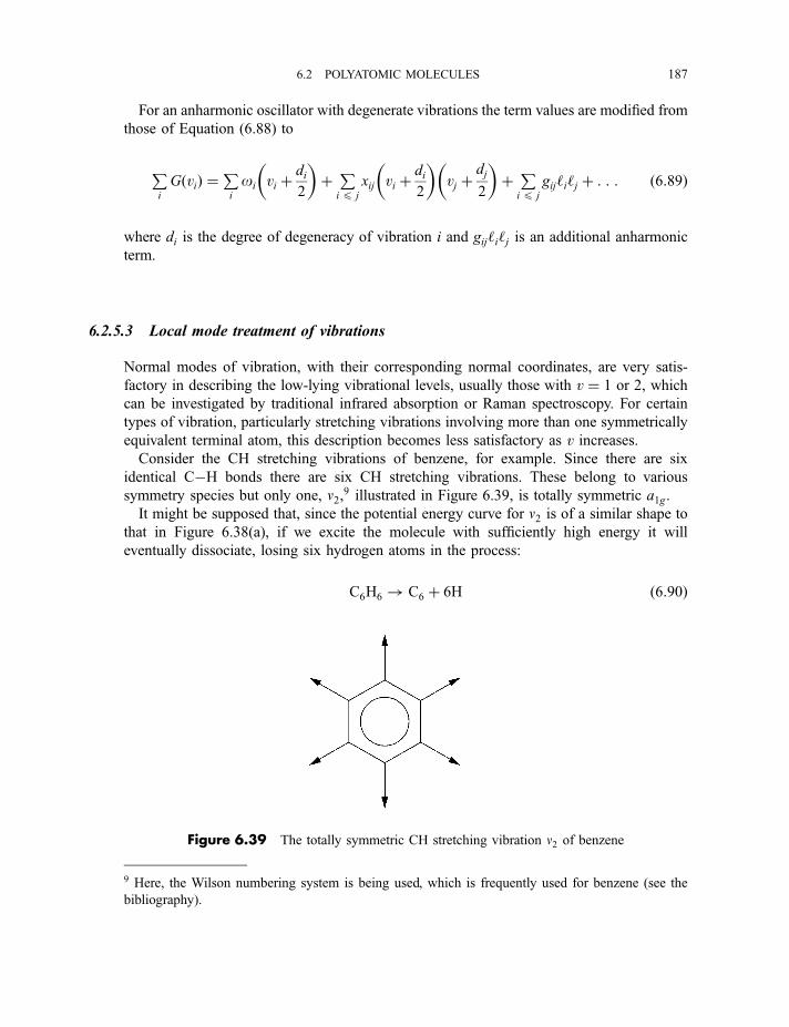
For an anharmonic oscillator with degenerate vibrations the term values are modified from
those of Equation (6.88) to
Pi
GðviÞ ¼Pi
oi vi þdi
2
� �þ P
i 4 j
xij vi þdi
2
� �vj þ
dj
2
� �þ P
i 4 j
gij‘i‘j þ : : : ð6:89Þ
where di is the degree of degeneracy of vibration i and gij‘i‘j is an additional anharmonic
term.
6.2.5.3 Local mode treatment of vibrations
Normal modes of vibration, with their corresponding normal coordinates, are very satis-
factory in describing the low-lying vibrational levels, usually those with v ¼ 1 or 2, which
can be investigated by traditional infrared absorption or Raman spectroscopy. For certain
types of vibration, particularly stretching vibrations involving more than one symmetrically
equivalent terminal atom, this description becomes less satisfactory as v increases.
Consider the CH stretching vibrations of benzene, for example. Since there are six
identical C�H bonds there are six CH stretching vibrations. These belong to various
symmetry species but only one, n2,9 illustrated in Figure 6.39, is totally symmetric a1g.
It might be supposed that, since the potential energy curve for n2 is of a similar shape to
that in Figure 6.38(a), if we excite the molecule with sufficiently high energy it will
eventually dissociate, losing six hydrogen atoms in the process:
C6H6! C6 þ 6H ð6:90Þ
Figure 6.39 The totally symmetric CH stretching vibration n2 of benzene
9 Here, the Wilson numbering system is being used, which is frequently used for benzene (see the
bibliography).
6.2 POLYATOMIC MOLECULES 187
This seems reasonable when we think only in terms of normal vibrations, but intuition
suggests that, since the dissociation in Equation (6.90) would require something like six
times the C�H bond dissociation energy (ca 66 412 kJ mol71), the process
C6H6! C6H5 þ H ð6:91Þ
is surely more likely to occur. This is indeed what happens but the difficulty is that no
normal vibration of benzene leads to CH stretching being localized in only one bond. A new
type of description of vibrational behaviour in such cases has been devised which is to treat
high overtone levels of CH stretching by a local mode, rather than a normal mode model.
Each C�H bond stretching is taken to behave as in the Morse model (Equation 6.23) which
describes fairly satisfactorily the anharmonic vibration of a diatomic molecule. The
extremely sensitive technique of photoacoustic spectroscopy has enabled transitions up to
v ¼ 6 in the CH stretching vibration to be observed and the transition wavenumbers have
been shown to fit those of a Morse oscillator quite well.
This local mode behaviour applies to vibrations of many other molecules with two or
more equivalent terminal atoms, and CO2 is such an example.
The probability of going, in Figure 6.35, from region B, where CO2 is in the equilibrium
configuration, to region C, in which it has lost both oxygen atoms, by exciting more and
more quanta of n1 and proceeding along the dashed line Q1, seems energetically unlikely.
The molecule will prefer to go from B to A1 (or A2), losing one oxygen atom only, by local
mode behaviour. Then it will go from A1 (or A2) to C by dissociation of CO. Therefore the
high overtone levels of CO stretching in CO2 will be better described by a local mode
model, involving anharmonic stretching of one C¼O bond, rather than a normal mode
model.
It should be realized, though, that either model can be used for levels for all values of v forsuch stretching vibrations but the normal mode model is more practically useful at low v andthe local mode model more useful at higher values of v.Although any stretching vibration involving symmetrically equivalent atoms should show
local mode behaviour at high v, the X�H stretching vibrations are more amenable to
investigation. The reason for this is that their vibrational quanta are large and, therefore, a
relatively low value of v is nearer to the dissociation energy than, say, for CF stretching
vibrations, and the transition probability decreases rapidly as v increases.
6.2.5.4 Vibrational potential functions with more than one minimum
The only types of anharmonic potential function we have encountered so far are the two
illustrated in Figure 6.38, both of which show only a single minimum. There are, however,
some vibrations whose potential functions do not resemble either of those but show more
than one minimum and whose term values are neither harmonic, nor are they given by
Equation (6.88) or Equation (6.89). Such vibrations can be separated into various types,
which will now be discussed individually.
188 6 VIBRATIONAL SPECTROSCOPY
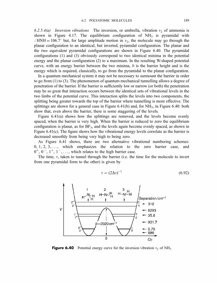
6.2.5.4(a) Inversion vibrations The inversion, or umbrella, vibration n2 of ammonia is
shown in Figure 4.17. The equilibrium configuration of NH3 is pyramidal with
ffHNH¼ 106.7� but, for large amplitude motion in n2, the molecule may go through the
planar configuration to an identical, but inverted, pyramidal configuration. The planar and
the two equivalent pyramidal configurations are shown in Figure 6.40. The pyramidal
configurations (1) and (3) obviously correspond to two identical minima in the potential
energy and the planar configuration (2) to a maximum. In the resulting W-shaped potential
curve, with an energy barrier between the two minima, b is the barrier height and is the
energy which is required, classically, to go from the pyramidal to the planar configuration.
In a quantum mechanical system it may not be necessary to surmount the barrier in order
to go from (1) to (3). The phenomenon of quantum mechanical tunnelling allows a degree of
penetration of the barrier. If the barrier is sufficiently low or narrow (or both) the penetration
may be so great that interaction occurs between the identical sets of vibrational levels in the
two limbs of the potential curve. This interaction splits the levels into two components, the
splitting being greater towards the top of the barrier where tunnelling is more effective. The
splittings are shown for a general case in Figure 6.41(b) and, for NH3, in Figure 6.40: both
show that, even above the barrier, there is some staggering of the levels.
Figure 6.41(a) shows how the splittings are removed, and the levels become evenly
spaced, when the barrier is very high. When the barrier is reduced to zero the equilibrium
configuration is planar, as for BF3, and the levels again become evenly spaced, as shown in
Figure 6.41(c). The figure shows how the vibrational energy levels correlate as the barrier is
decreased smoothly from being very high to being zero.
As Figure 6.41 shows, there are two alternative vibrational numbering schemes:
0, 1, 2, 3, . . . , which emphasizes the relation to the zero barrier case, and
0þ, 07, 1þ, 17, . . . , which relates to the high barrier case.
The time, t, taken to tunnel through the barrier (i.e. the time for the molecule to invert
from one pyramidal form to the other) is given by
t ¼ ð2DnÞ�1 ð6:92Þ
Figure 6.40 Potential energy curve for the inversion vibration n2 of NH3
6.2 POLYATOMIC MOLECULES 189
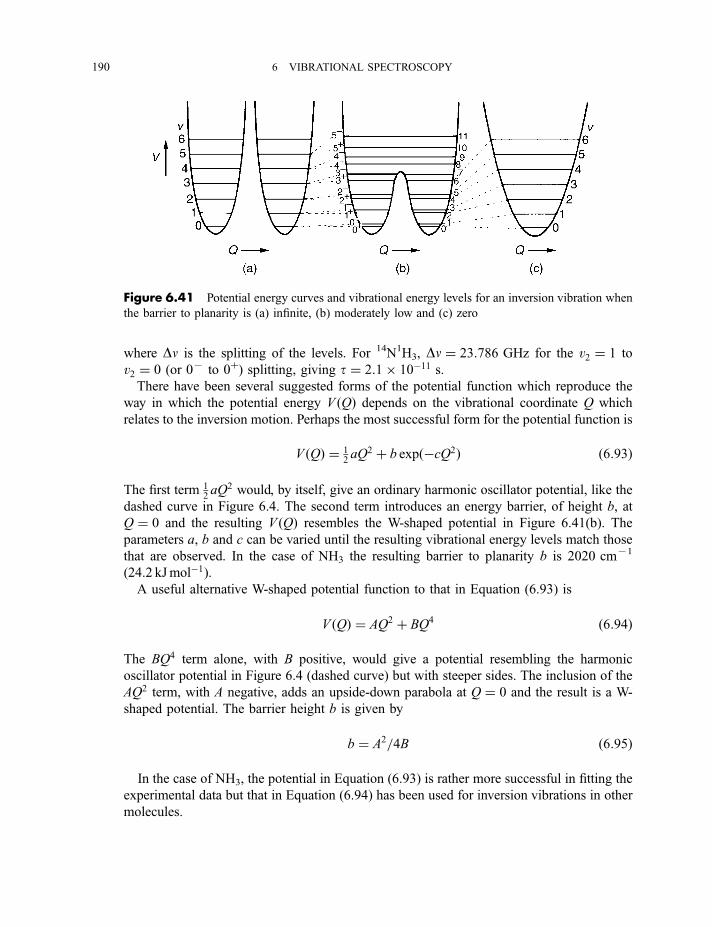
where Dn is the splitting of the levels. For 14N1H3, Dn ¼ 23:786 GHz for the v2 ¼ 1 to
v2 ¼ 0 (or 07 to 0þ) splitting, giving t ¼ 2:1� 10�11 s.There have been several suggested forms of the potential function which reproduce the
way in which the potential energy V ðQÞ depends on the vibrational coordinate Q which
relates to the inversion motion. Perhaps the most successful form for the potential function is
V ðQÞ ¼ 12aQ2 þ b expð�cQ2Þ ð6:93Þ
The first term 12aQ2 would, by itself, give an ordinary harmonic oscillator potential, like the
dashed curve in Figure 6.4. The second term introduces an energy barrier, of height b, at
Q ¼ 0 and the resulting V ðQÞ resembles the W-shaped potential in Figure 6.41(b). The
parameters a, b and c can be varied until the resulting vibrational energy levels match those
that are observed. In the case of NH3 the resulting barrier to planarity b is 2020 cm71
(24.2 kJmol�1).A useful alternative W-shaped potential function to that in Equation (6.93) is
V ðQÞ ¼ AQ2 þ BQ4 ð6:94Þ
The BQ4 term alone, with B positive, would give a potential resembling the harmonic
oscillator potential in Figure 6.4 (dashed curve) but with steeper sides. The inclusion of the
AQ2 term, with A negative, adds an upside-down parabola at Q ¼ 0 and the result is a W-
shaped potential. The barrier height b is given by
b ¼ A2=4B ð6:95Þ
In the case of NH3, the potential in Equation (6.93) is rather more successful in fitting the
experimental data but that in Equation (6.94) has been used for inversion vibrations in other
molecules.
Figure 6.41 Potential energy curves and vibrational energy levels for an inversion vibration when
the barrier to planarity is (a) infinite, (b) moderately low and (c) zero
190 6 VIBRATIONAL SPECTROSCOPY
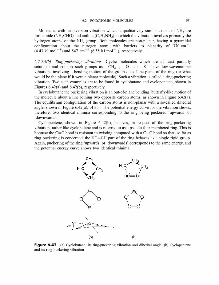
Molecules with an inversion vibration which is qualitatively similar to that of NH3 are
formamide (NH2CHO) and aniline (C6H5NH2) in which the vibration involves primarily the
hydrogen atoms of the NH2 group. Both molecules are non-planar, having a pyramidal
configuration about the nitrogen atom, with barriers to planarity of 370 cm71
(4.43 kJ mol71) and 547 cm71 (6.55 kJ mol71), respectively.
6.2.5.4(b) Ring-puckering vibrations Cyclic molecules which are at least partially
saturated and contain such groups as �CH2�, �O� or �S� have low-wavenumber
vibrations involving a bending motion of the group out of the plane of the ring (or what
would be the plane if it were a planar molecule). Such a vibration is called a ring-puckering
vibration. Two such examples are to be found in cyclobutane and cyclopentene, shown in
Figures 6.42(a) and 6.42(b), respectively.
In cyclobutane the puckering vibration is an out-of-plane bending, butterfly-like motion of
the molecule about a line joining two opposite carbon atoms, as shown in Figure 6.42(a).
The equilibrium configuration of the carbon atoms is non-planar with a so-called dihedral
angle, shown in Figure 6.42(a), of 35�. The potential energy curve for the vibration shows,
therefore, two identical minima corresponding to the ring being puckered ‘upwards’ or
‘downwards’.
Cyclopentene, shown in Figure 6.42(b), behaves, in respect of the ring-puckering
vibration, rather like cyclobutane and is referred to as a pseudo four-membered ring. This is
because the C¼C bond is resistant to twisting compared with a C�C bond so that, so far as
ring puckering is concerned, the HC¼CH part of the ring behaves as a single rigid group.
Again, puckering of the ring ‘upwards’ or ‘downwards’ corresponds to the same energy, and
the potential energy curve shows two identical minima.
Figure 6.42 (a) Cyclobutane, its ring-puckering vibration and dihedral angle. (b) Cyclopentene
and its ring-puckering vibration
6.2 POLYATOMIC MOLECULES 191
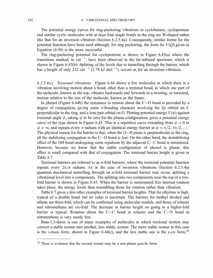
The potential energy curves for ring-puckering vibrations in cyclobutane, cyclopentene
and similar cyclic molecules with at least four single bonds in the ring are W-shaped rather
like that for an inversion vibration (Section 6.2.5.4a). Consequently, similar forms for the
potential function have been used although, for ring puckering, the form for V ðQÞ given in
Equation (6.94) is the more successful.
The ring-puckering potential for cyclopentene is shown in Figure 6.43(a) where the
transitions marked, in cm71, have been observed in the far-infrared spectrum, which is
shown in Figure 6.43(b). Splitting of the levels due to tunnelling through the barrier, which
has a height of only 232 cm71 (2.78 kJ mol71), occurs as for an inversion vibration.
6.2.5.4(c) Torsional vibrations Figure 6.44 shows a few molecules in which there is a
vibration involving motion about a bond, other than a terminal bond, in which one part of
the molecule, known as the top, vibrates backwards and forwards in a twisting, or torsional,
motion relative to the rest of the molecule, known as the frame.
In phenol (Figure 6.44b) the resistance to torsion about the C�O bond is provided by a
degree of conjugation, giving some p-bonding character involving the 2p orbital on C
perpendicular to the ring, and a lone pair orbital on O. Plotting potential energy V ðfÞ againsttorsional angle f, taking f to be zero for the planar configuration, gives a potential energy
curve of the type shown in Figure 6.45. This is a repetitive curve extending from f ¼ 0 to
f ¼ 1 and repeats every p radians with an identical energy barrier at f ¼ p=2, 3p=2, . . . .The physical reason for the barrier is that, when the O�H plane is perpendicular to the ring,
all the stabilizing conjugation in the C�O bond is lost. On the other hand, the destabilizing
effect of the OH bond undergoing some repulsion by the adjacent C�C bond is minimized.
However, because we know that the stable configuration of phenol is planar, this
effect is small compared with that of conjugation. The torsional barrier height is given in
Table 6.7.
Torsional barriers are referred to as n-fold barriers, where the torsional potential function
repeats every 2p=n radians. As in the case of inversion vibrations (Section 6.2.5.4a)
quantum mechanical tunnelling through an n-fold torsional barrier may occur, splitting a
vibrational level into n components. The splitting into two components near the top of a two-
fold barrier is shown in Figure 6.45. When the barrier is surmounted free internal rotation
takes place, the energy levels then resembling those for rotation rather than vibration.
Table 6.7 gives a few other examples of torsional barrier heights. That for ethylene is high,
typical of a double bond, but its value is uncertain. The barriers for methyl alcohol and
ethane are three-fold, which can be confirmed using molecular models, and those of toluene
and nitromethane are six-fold. The decrease in barrier height on going to a higher-fold
barrier is typical. Rotation about the C�C bond in toluene and the C�N bond in
nitromethane is very nearly free.
Buta-1,3-diene is one of many examples of molecules in which torsional motion may
convert a stable isomer into another, less stable, isomer. The more stable isomer in this case
is the s-trans form, shown in Figure 6.44(e), and the less stable one is the s-cis form,10
10 There is evidence that the second isomer may be a non-planar gauche form.
192 6 VIBRATIONAL SPECTROSCOPY
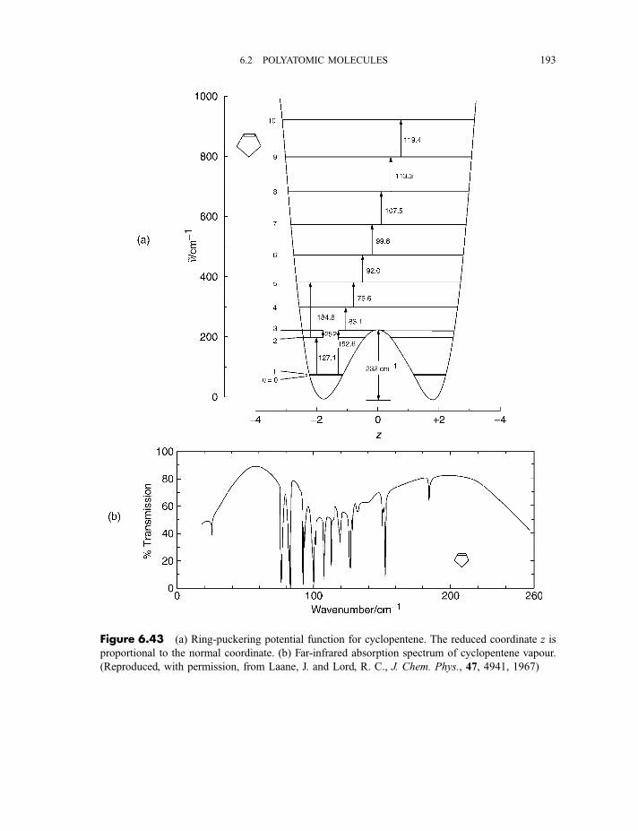
Figure 6.43 (a) Ring-puckering potential function for cyclopentene. The reduced coordinate z is
proportional to the normal coordinate. (b) Far-infrared absorption spectrum of cyclopentene vapour.
(Reproduced, with permission, from Laane, J. and Lord, R. C., J. Chem. Phys., 47, 4941, 1967)
6.2 POLYATOMIC MOLECULES 193
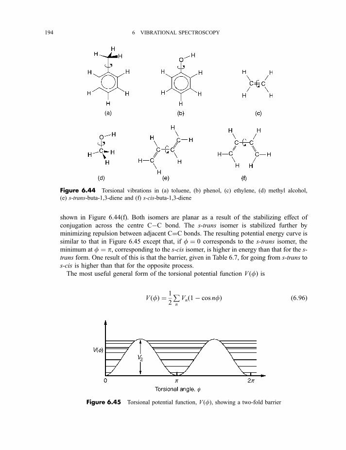
shown in Figure 6.44(f). Both isomers are planar as a result of the stabilizing effect of
conjugation across the centre C�C bond. The s-trans isomer is stabilized further by
minimizing repulsion between adjacent C¼C bonds. The resulting potential energy curve is
similar to that in Figure 6.45 except that, if f ¼ 0 corresponds to the s-trans isomer, the
minimum at f ¼ p, corresponding to the s-cis isomer, is higher in energy than that for the s-
trans form. One result of this is that the barrier, given in Table 6.7, for going from s-trans to
s-cis is higher than that for the opposite process.
The most useful general form of the torsional potential function V ðfÞ is
V ðfÞ ¼ 1
2
Pn
Vnð1� cos nfÞ ð6:96Þ
Figure 6.44 Torsional vibrations in (a) toluene, (b) phenol, (c) ethylene, (d) methyl alcohol,
(e) s-trans-buta-1,3-diene and (f) s-cis-buta-1,3-diene
Figure 6.45 Torsional potential function, V ðfÞ, showing a two-fold barrier
194 6 VIBRATIONAL SPECTROSCOPY
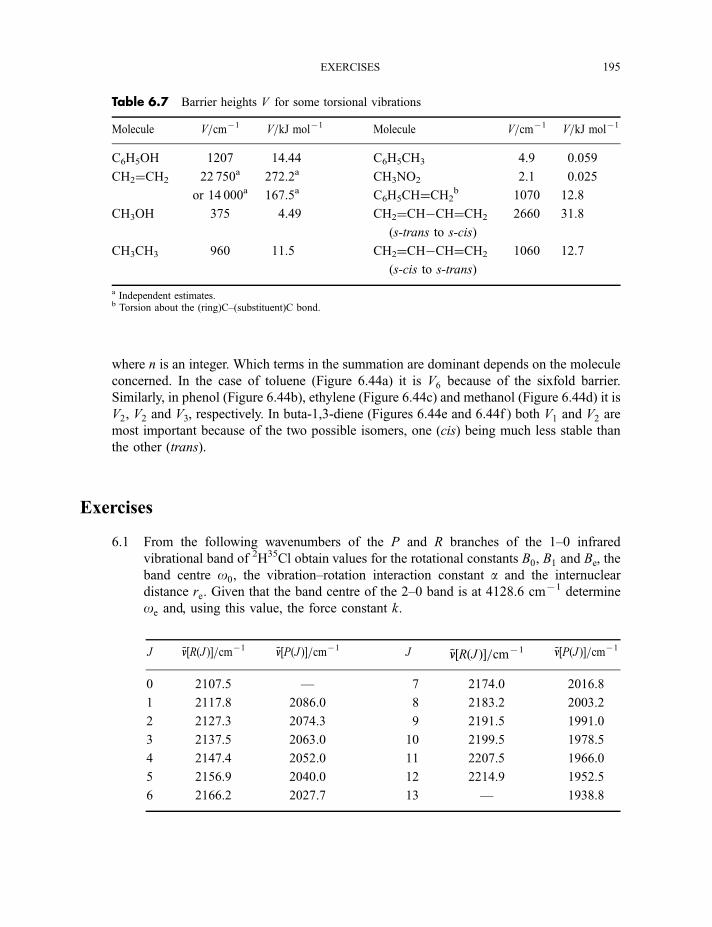
where n is an integer. Which terms in the summation are dominant depends on the molecule
concerned. In the case of toluene (Figure 6.44a) it is V6 because of the sixfold barrier.
Similarly, in phenol (Figure 6.44b), ethylene (Figure 6.44c) and methanol (Figure 6.44d) it is
V2, V2 and V3, respectively. In buta-1,3-diene (Figures 6.44e and 6.44f ) both V1 and V2 are
most important because of the two possible isomers, one (cis) being much less stable than
the other (trans).
Exercises
6.1 From the following wavenumbers of the P and R branches of the 1–0 infrared
vibrational band of 2H35Cl obtain values for the rotational constants B0, B1 and Be, the
band centre o0, the vibration–rotation interaction constant a and the internuclear
distance re. Given that the band centre of the 2–0 band is at 4128.6 cm71 determine
oe and, using this value, the force constant k.
J ~nn½RðJ Þ�=cm71 ~nn½PðJ Þ�=cm71 J ~nn½RðJ Þ�=cm71 ~nn½PðJ Þ�=cm71
0 2107.5 — 7 2174.0 2016.8
1 2117.8 2086.0 8 2183.2 2003.2
2 2127.3 2074.3 9 2191.5 1991.0
3 2137.5 2063.0 10 2199.5 1978.5
4 2147.4 2052.0 11 2207.5 1966.0
5 2156.9 2040.0 12 2214.9 1952.5
6 2166.2 2027.7 13 — 1938.8
Table 6.7 Barrier heights V for some torsional vibrations
Molecule V=cm71 V=kJ mol71 Molecule V=cm71 V=kJ mol71
C6H5OH 1207 14.44 C6H5CH3 4.9 0.059
CH2¼CH2 22 750a 272.2a CH3NO2 2.1 0.025
or 14 000a 167.5a C6H5CH¼CH2b 1070 12.8
CH3OH 375 4.49 CH2¼CH�CH¼CH2 2660 31.8
(s-trans to s-cis)
CH3CH3 960 11.5 CH2¼CH�CH¼CH2 1060 12.7
(s-cis to s-trans)
a Independent estimates.b Torsion about the (ring)C–(substituent)C bond.
EXERCISES 195
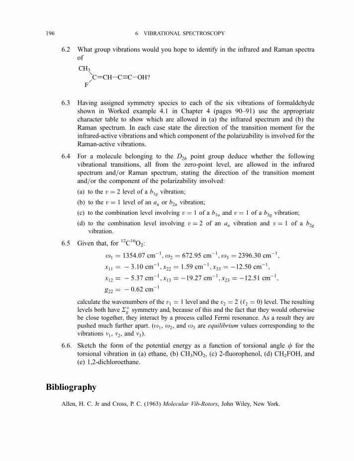
6.2 What group vibrations would you hope to identify in the infrared and Raman spectra
of
6.3 Having assigned symmetry species to each of the six vibrations of formaldehyde
shown in Worked example 4.1 in Chapter 4 (pages 90–91) use the appropriate
character table to show which are allowed in (a) the infrared spectrum and (b) the
Raman spectrum. In each case state the direction of the transition moment for the
infrared-active vibrations and which component of the polarizability is involved for the
Raman-active vibrations.
6.4 For a molecule belonging to the D2h point group deduce whether the following
vibrational transitions, all from the zero-point level, are allowed in the infrared
spectrum and=or Raman spectrum, stating the direction of the transition moment
and=or the component of the polarizability involved:
(a) to the v ¼ 2 level of a b1g vibration;
(b) to the v ¼ 1 level of an au or b2u vibration;
(c) to the combination level involving v ¼ 1 of a b1u and v ¼ 1 of a b3g vibration;
(d) to the combination level involving v ¼ 2 of an au vibration and v ¼ 1 of a b2gvibration.
6.5 Given that, for 12C16O2:
o1 ¼ 1354:07 cm�1;o2 ¼ 672:95 cm�1;o3 ¼ 2396:30 cm�1;
x11 ¼ � 3:10 cm�1; x22 ¼ 1:59 cm�1; x33 ¼ �12:50 cm�1;
x12 ¼ � 5:37 cm�1; x13 ¼ �19:27 cm�1; x23 ¼ �12:51 cm�1;
g22 ¼ � 0:62 cm�1
calculate the wavenumbers of the v1 ¼ 1 level and the v2 ¼ 2 ð‘2 ¼ 0Þ level. The resultinglevels both have Sþg symmetry and, because of this and the fact that they would otherwise
be close together, they interact by a process called Fermi resonance. As a result they are
pushed much further apart. (o1, o2, and o3 are equilibrium values corresponding to the
vibrations n1, n2, and n3).
6.6. Sketch the form of the potential energy as a function of torsional angle f for the
torsional vibration in (a) ethane, (b) CH3NO2, (c) 2-fluorophenol, (d) CH2FOH, and
(e) 1,2-dichloroethane.
Bibliography
Allen, H. C. Jr and Cross, P. C. (1963) Molecular Vib-Rotors, John Wiley, New York.
C CH C C OH?CH3
F
196 6 VIBRATIONAL SPECTROSCOPY

Bellamy, L. J. (1980) The Infrared Spectra of Complex Molecules, Volume 2: Advances in Infrared
Group Frequencies, Chapman and Hall, London.
Duxbury, G. (1999) Infrared Vibration–Rotation Spectroscopy, John Wiley, Chichester.
Gans, P. (1971) Vibrating Molecules, Chapman and Hall, London.
Herzberg, G. (1989) Spectra of Diatomic Molecules, Krieger, Florida.
Herzberg, G. (1991) Infrared and Raman Spectra of Polyatomic Molecules, Krieger, Florida.
Long, D. A. (2002) The Raman Effect, John Wiley, Chichester.
Schrader, B. (1995) Infrared and Raman Spectroscopy, Wiley-VCH, Weinheim.
Wilson, E. B. Jr (1934) Phys. Rev., 45, 706.
Wilson, E. B. Jr, Decius, J. C. and Cross, P. C. (1980) Molecular Vibrations, Dover, New York.
Woodward, L. A. (1972) Introduction to the Theory of Molecular Vibrations and Vibrational
Spectroscopy, Oxford University Press, Oxford.
BIBLIOGRAPHY 197

7Electronic Spectroscopy
7.1 Atomic spectroscopy
Electronic spectroscopy is the study of transitions, in absorption or emission, between
electronic states of an atom or molecule. Atoms are unique in this respect as they have only
electronic degrees of freedom, apart from translation and nuclear spin, whereas molecules
have, in addition, vibrational and rotational degrees of freedom. One result is that electronic
spectra of atoms are very much simpler in appearance than those of molecules.
7.1.1 The periodic table
For the hydrogen atom, and for the hydrogen-like ions such as Heþ, Li2þ, . . . , with a single
electron in the field of a nucleus with charge þ Ze, the hamiltonian (the quantum
mechanical form of the energy) is given by
H ¼ h2
2mH2 � Ze2
4pe0rð7:1Þ
analogous to Equation (1.30) for the hydrogen atom, where the terms are explained.
For a polyelectronic atom the hamiltonian becomes
H ¼ � h2
2me
Pi
H2i �
Pi
Ze2
4pe0riþ P
i < j
e2
4pe0rijð7:2Þ
where the summation is over all electrons i. The first two terms are simply sums of terms like
those for one electron in Equation (7.1). The third term is new and is added because of
coulombic repulsions between all possible pairs of electrons a distance rij apart. It is in
contrast to the second term, which represents the coulombic attraction between each electron
and the nucleus at a distance ri.
Because of the electron–electron repulsion term in Equation (7.2) the hamiltonian cannot
be broken down into a sum of contributions from each electron and the Schrodinger
199
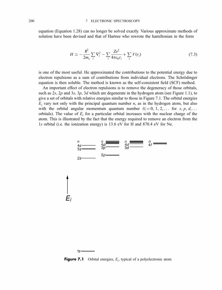
equation (Equation 1.28) can no longer be solved exactly. Various approximate methods of
solution have been devised and that of Hartree who rewrote the hamiltonian in the form
H ’ � h2
2me
Pi
H2i �
Pi
Ze2
4pe0riþP
i
V ðriÞ ð7:3Þ
is one of the most useful. He approximated the contributions to the potential energy due to
electron repulsions as a sum of contributions from individual electrons. The Schrodinger
equation is then soluble. The method is known as the self-consistent field (SCF) method.
An important effect of electron repulsions is to remove the degeneracy of those orbitals,
such as 2s, 2p and 3s, 3p, 3d which are degenerate in the hydrogen atom (see Figure 1.1), to
give a set of orbitals with relative energies similar to those in Figure 7.1. The orbital energies
Ei vary not only with the principal quantum number n, as in the hydrogen atom, but also
with the orbital angular momentum quantum number ‘(¼ 0, 1, 2, . . . for s, p, d, . . .orbitals). The value of Ei for a particular orbital increases with the nuclear charge of the
atom. This is illustrated by the fact that the energy required to remove an electron from the
1s orbital (i.e. the ionization energy) is 13.6 eV for H and 870.4 eV for Ne.
Figure 7.1 Orbital energies, Ei, typical of a polyelectronic atom
200 7 ELECTRONIC SPECTROSCOPY
Electrons in the atom concerned may be fed into the orbitals in Figure 7.1 in order of
increasing energy until the electrons are used up, to give what is referred to as the ground
configuration of the atom. This feeding in of the electrons in order of increasing orbital
energy follows the aufbau or building-up principle, but must also obey the Pauli exclusion
principle. This states that no two electrons can have the same set of quantum numbers n, ‘,m‘, ms. Since m‘ can take ð2‘þ 1Þ values (see Equation 1.45) and ms ¼ � 1
2(see Equation
1.47), each orbital characterized by particular values of n and ‘ can accommodate 2ð2‘þ 1Þelectrons. It follows that an ns orbital with ‘ ¼ 0 can accommodate two electrons, an np
orbital with ‘ ¼ 1 can take six, an nd orbital with ‘ ¼ 2 can take ten, and so on.
Whereas an orbital refers to a particular set of values of n and ‘, a shell refers to all orbitalshaving the same value of n. For n¼ 1, 2, 3, 4, . . . the shells are labelled K, L, M, N, . . . .The distinction between a configuration and a state is an important one. A configuration
describes the way in which the electrons are distributed among various orbitals but a
configuration may give rise to more than one state. For example, as we shall see in Section
7.1.2.3(b), the ground configuration 1s22s22p2 of the carbon atom gives rise to three
electronic states of different energies.
Table 7.1 gives the ground configurations and other useful data for all the elements. This
table illustrates features which are common to the electron configurations of elements which
are known to be chemically similar. The alkali metals, Li, Na, K, Rb and Cs, all have an
outer ns1 configuration consistent with their being monovalent, and the alkaline earth metals,
Be, Mg, Ca, Sr and Ba, all have an outer ns2 configuration and are divalent. The noble (inert
or rare) gases, Ne, Ar, Kr, Xe and Rn, all have an outer np6 configuration, the filled orbital
(or sub-shell, as it is sometimes called) conferring chemical inertness, and the filled K shell
in He has a similar effect.
The first transition series, Sc, Ti, V, Cr, Mn, Fe, Co, Ni, Cu and Zn, is characterized by the
filling up of the 3d orbital. Figure 7.1 shows that the 3d and 4s orbitals are very similar in
energy, but their separation changes along the series. The result is that, although there is a
preference by most of these elements for having two electrons in the 4s orbital, Cu has a
. . . 3d104s1 ground configuration because of the innate stability associated with a filled 3d
orbital. There is also some stability associated with a half-filled orbital (2p3, 3d 5, etc.)
resulting in the . . . 3d54s1 ground configuration of Cr. There is no simple reason for the
stability of the half-filled orbital but, when this occurs, all electrons have parallel spins (i.e.
all have ms ¼ þ 12or ms ¼ � 1
2) and this situation modifies the electron–nucleus interactions
resulting in a lowering of the energy.
Filling up the 4f orbital is a feature of the lanthanides. The 4f and 5d orbitals are of
similar energy so that occasionally, as in La, Ce and Gd, one electron goes into 5d rather
than 4f . Similarly, in the actinides, Ac to No, the 5f subshell is filled in competition with 6d.
7.1.2 Vector representation of momenta and vector coupling approximations
7.1.2.1 Angular momenta and magnetic moments
We saw in Section 1.3.2 and in Figure 1.5 how the orbital angular momentum of an electron can
be represented by a vector, the direction of which is determined by the right-hand screw rule.
7.1 ATOMIC SPECTROSCOPY 201
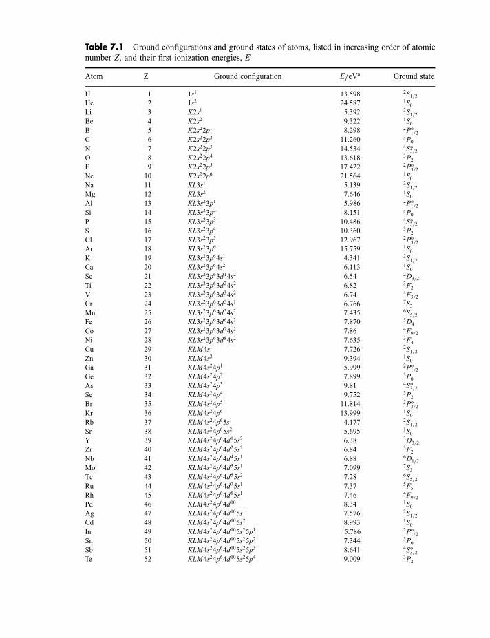
Table 7.1 Ground configurations and ground states of atoms, listed in increasing order of atomic
number Z, and their first ionization energies, E
Atom Z Ground configuration E=eVa Ground state
H 1 1s1 13.598 2S1=2He 2 1s2 24.587 1S0Li 3 K2s1 5.392 2S1=2Be 4 K2s2 9.322 1S0B 5 K2s22p1 8.298 2Po
1=2
C 6 K2s22p2 11.260 3P0
N 7 K2s22p3 14.534 4So3=2O 8 K2s22p4 13.618 3P2
F 9 K2s22p5 17.422 2Po3=2
Ne 10 K2s22p6 21.564 1S0Na 11 KL3s1 5.139 2S1=2Mg 12 KL3s2 7.646 1S0Al 13 KL3s23p1 5.986 2Po
1=2
Si 14 KL3s23p2 8.151 3P0
P 15 KL3s23p3 10.486 4So3=2S 16 KL3s23p4 10.360 3P2
Cl 17 KL3s23p5 12.967 2Po3=2
Ar 18 KL3s23p6 15.759 1S0K 19 KL3s23p64s1 4.341 2S1=2Ca 20 KL3s23p64s2 6.113 1S0Sc 21 KL3s23p63d14s2 6.54 2D3=2
Ti 22 KL3s23p63d24s2 6.82 3F2
V 23 KL3s23p63d34s2 6.74 4F3=2
Cr 24 KL3s23p63d54s1 6.766 7S3Mn 25 KL3s23p63d54s2 7.435 6S5=2Fe 26 KL3s23p63d64s2 7.870 5D4
Co 27 KL3s23p63d74s2 7.86 4F9=2
Ni 28 KL3s23p63d84s2 7.635 3F4
Cu 29 KLM4s1 7.726 2S1=2Zn 30 KLM4s2 9.394 1S0Ga 31 KLM4s24p1 5.999 2Po
1=2
Ge 32 KLM4s24p2 7.899 3P0
As 33 KLM4s24p3 9.81 4So3=2Se 34 KLM4s24p4 9.752 3P2
Br 35 KLM4s24p5 11.814 2Po3=2
Kr 36 KLM4s24p6 13.999 1S0Rb 37 KLM4s24p65s1 4.177 2S1=2Sr 38 KLM4s24p65s2 5.695 1S0Y 39 KLM4s24p64d15s2 6.38 3D3=2
Zr 40 KLM4s24p64d25s2 6.84 3F2
Nb 41 KLM4s24p64d45s1 6.88 6D1=2
Mo 42 KLM4s24p64d55s1 7.099 7S3Tc 43 KLM4s24p64d55s2 7.28 6S5=2Ru 44 KLM4s24p64d75s1 7.37 5F5
Rh 45 KLM4s24p64d85s1 7.46 4F9=2
Pd 46 KLM4s24p64d10 8.34 1S0Ag 47 KLM4s24p64d105s1 7.576 2S1=2Cd 48 KLM4s24p64d105s2 8.993 1S0In 49 KLM4s24p64d105s25p1 5.786 2Po
1=2
Sn 50 KLM4s24p64d105s25p2 7.344 3P0
Sb 51 KLM4s24p64d105s25p3 8.641 4So3=2Te 52 KLM4s24p64d105s25p4 9.009 3P2
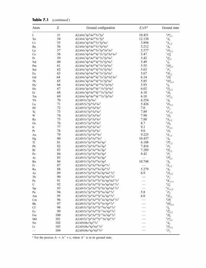
Table 7.1 (continued )
Atom Z Ground configuration E=eVa Ground state
I 53 KLM4s24p64d105s25p5 10.451 2Po3=2
Xe 54 KLM4s24p64d105s25p6 12.130 1S0Cs 55 KLM4s24p64d105s25p66s1 3.894 2S1=2Ba 56 KLM4s24p64d105s25p66s2 5.212 1S0La 57 KLM4s24p64d105s25p65d16s2 5.577 2D3=2
Ce 58 KLM4s24p64d104f 15s25p65d16s2 5.47 1Go4
Pr 59 KLM4s24p64d104f 35s25p66s2 5.42 4Io9=2Nd 60 KLM4s24p64d104f 45s25p66s2 5.49 5I4Pm 61 KLM4s24p64d104f 55s25p66s2 5.55 6Ho
5=2
Sm 62 KLM4s24p64d104f 65s25p66s2 5.63 7F0
Eu 63 KLM4s24p64d104f 75s25p66s2 5.67 8So7=2Gd 64 KLM4s24p64d104f 75s25p65d16s2 6.14 9Do
2
Tb 65 KLM4s24p64d104f 95s25p66s2 5.85 6Ho15=2
Dy 66 KLM4s24p64d104f 105s25p66s2 5.93 5I8Ho 67 KLM4s24p64d104f 115s25p66s2 6.02 4Io15=2Er 68 KLM4s24p64d104f 125s25p66s2 6.10 3H6
Tm 69 KLM4s24p64d104f 135s25p66s2 6.18 2Fo7=2
Yb 70 KLMN5s25p66s2 6.254 1S0Lu 71 KLMN5s25p65d16s2 5.426 2D3=2
Hf 72 KLMN5s25p65d26s2 7.0 3F2
Ta 73 KLMN5s25p65d36s2 7.89 4F3=2
W 74 KLMN5s25p65d46s2 7.98 5D0
Re 75 KLMN5s25p65d56s2 7.88 6S5=2Os 76 KLMN5s25p65d66s2 8.7 5D4
Ir 77 KLMN5s25p65d76s2 9.1 4F9=2
Pt 78 KLMN5s25p65d96s1 9.0 3D3
Au 79 KLMN5s25p65d106s1 9.225 2S1=2Hg 80 KLMN5s25p65d106s2 10.437 1S0Tl 81 KLMN5s25p65d106s26p1 6.108 2Po
1=2
Pb 82 KLMN5s25p65d106s26p2 7.416 3P0
Bi 83 KLMN5s25p65d106s26p3 7.289 4So3=2Po 84 KLMN5s25p65d106s26p4 8.42 3P2
At 85 KLMN5s25p65d106s26p5 — 2Po3=2
Rn 86 KLMN5s25p65d106s26p6 10.748 1S0Fr 87 KLMN5s25p65d106s26p67s1 — 2S1=2Ra 88 KLMN5s25p65d106s26p67s2 5.279 1S0Ac 89 KLMN5s25p65d106s26p66d17s2 6.9 2D3=2
Th 90 KLMN5s25p65d106s26p66d27s2 — 3F2
Pa 91 KLMN5s25p65d105f 26s26p66d17s2 — 4K11=2
U 92 KLMN5s25p65d105f 36s26p66d17s2 — 5Lo6Np 93 KLMN5s25p65d105f 46s26p66d17s2 — 6L11=2Pu 94 KLMN5s25p65d105f 66s26p67s2 5.8 7F0
Am 95 KLMN5s25p65d105f 76s26p67s2 6.0 8So7=2Cm 96 KLMN5s25p65d105f 76s26p66d17s2 — 9Do
2
Bk 97 KLMN5s25p65d105f 96s26p67s2 — 6Ho15=2
Cf 98 KLMN5s25p65d105f 106s26p67s2 — 5I8Es 99 KLMN5s25p65d105f 116s26p67s2 — 4I015=2Fm 100 KLMN5s25p65d105f 126s26p67s2 — 3H6
Md 101 KLMN5s25p65d105f 136s26p67s2 — 2Fo3=2
No 102 KLMNO6s26p67s2 — 1S0Lr 103 KLMNO6s26p66d17s2 — 2D3=2
— 104 KLMNO6s26p66d27s2 — 3F2
a For the process A! Aþ þ e, where Aþ is in its ground state.
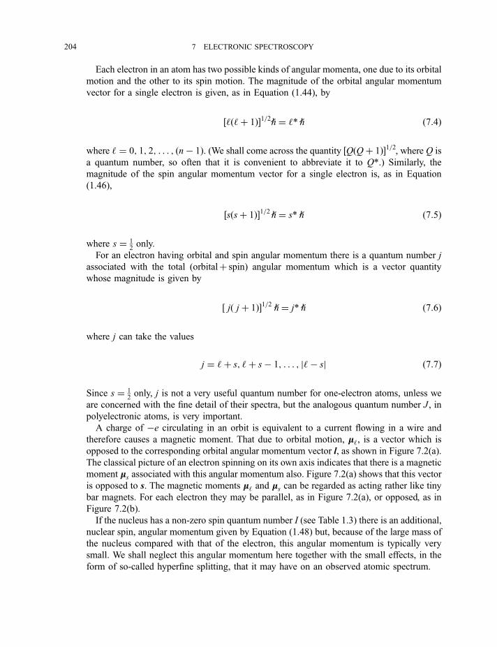
Each electron in an atom has two possible kinds of angular momenta, one due to its orbital
motion and the other to its spin motion. The magnitude of the orbital angular momentum
vector for a single electron is given, as in Equation (1.44), by
½‘ð‘þ 1Þ�1=2h ¼ ‘* h ð7:4Þ
where ‘ ¼ 0; 1; 2; . . . ; ðn� 1Þ. (We shall come across the quantity ½QðQþ 1Þ�1=2, where Q is
a quantum number, so often that it is convenient to abbreviate it to Q*.) Similarly, the
magnitude of the spin angular momentum vector for a single electron is, as in Equation
(1.46),
½sðsþ 1Þ�1=2h ¼ s* h ð7:5Þ
where s ¼ 12only.
For an electron having orbital and spin angular momentum there is a quantum number j
associated with the total (orbitalþ spin) angular momentum which is a vector quantity
whose magnitude is given by
½ jð j þ 1Þ�1=2 h ¼ j* h ð7:6Þ
where j can take the values
j ¼ ‘þ s; ‘þ s� 1; . . . ; j‘� sj ð7:7Þ
Since s ¼ 12only, j is not a very useful quantum number for one-electron atoms, unless we
are concerned with the fine detail of their spectra, but the analogous quantum number J , in
polyelectronic atoms, is very important.
A charge of �e circulating in an orbit is equivalent to a current flowing in a wire and
therefore causes a magnetic moment. That due to orbital motion, mm‘, is a vector which is
opposed to the corresponding orbital angular momentum vector l, as shown in Figure 7.2(a).
The classical picture of an electron spinning on its own axis indicates that there is a magnetic
moment mms associated with this angular momentum also. Figure 7.2(a) shows that this vector
is opposed to s. The magnetic moments mm‘ and mms can be regarded as acting rather like tiny
bar magnets. For each electron they may be parallel, as in Figure 7.2(a), or opposed, as in
Figure 7.2(b).
If the nucleus has a non-zero spin quantum number I (see Table 1.3) there is an additional,
nuclear spin, angular momentum given by Equation (1.48) but, because of the large mass of
the nucleus compared with that of the electron, this angular momentum is typically very
small. We shall neglect this angular momentum here together with the small effects, in the
form of so-called hyperfine splitting, that it may have on an observed atomic spectrum.
204 7 ELECTRONIC SPECTROSCOPY
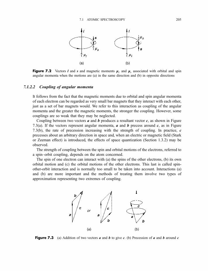
7.1.2.2 Coupling of angular momenta
It follows from the fact that the magnetic moments due to orbital and spin angular momenta
of each electron can be regarded as very small bar magnets that they interact with each other,
just as a set of bar magnets would. We refer to this interaction as coupling of the angular
momenta and the greater the magnetic moments, the stronger the coupling. However, some
couplings are so weak that they may be neglected.
Coupling between two vectors a and b produces a resultant vector c, as shown in Figure
7.3(a). If the vectors represent angular momenta, a and b precess around c, as in Figure
7.3(b), the rate of precession increasing with the strength of coupling. In practice, c
precesses about an arbitrary direction in space and, when an electric or magnetic field (Stark
or Zeeman effect) is introduced, the effects of space quantization (Section 1.3.2) may be
observed.
The strength of coupling between the spin and orbital motions of the electrons, referred to
a spin–orbit coupling, depends on the atom concerned.
The spin of one electron can interact with (a) the spins of the other electrons, (b) its own
orbital motion and (c) the orbital motions of the other electrons. This last is called spin-
other-orbit interaction and is normally too small to be taken into account. Interactions (a)
and (b) are more important and the methods of treating them involve two types of
approximation representing two extremes of coupling.
Figure 7.2 Vectors l and s and magnetic moments mm‘ and mms associated with orbital and spin
angular momenta when the motions are (a) in the same direction and (b) in opposite directions
Figure 7.3 (a) Addition of two vectors a and b to give c. (b) Precession of a and b around c
7.1 ATOMIC SPECTROSCOPY 205
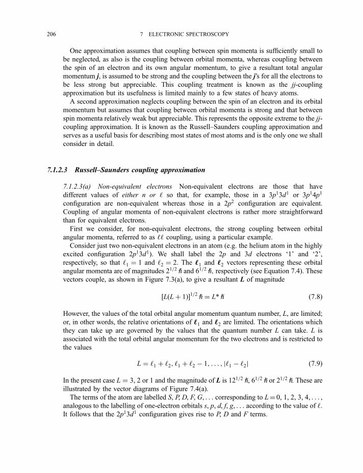
One approximation assumes that coupling between spin momenta is sufficiently small to
be neglected, as also is the coupling between orbital momenta, whereas coupling between
the spin of an electron and its own angular momentum, to give a resultant total angular
momentum j, is assumed to be strong and the coupling between the j’s for all the electrons to
be less strong but appreciable. This coupling treatment is known as the jj-coupling
approximation but its usefulness is limited mainly to a few states of heavy atoms.
A second approximation neglects coupling between the spin of an electron and its orbital
momentum but assumes that coupling between orbital momenta is strong and that between
spin momenta relatively weak but appreciable. This represents the opposite extreme to the jj-
coupling approximation. It is known as the Russell–Saunders coupling approximation and
serves as a useful basis for describing most states of most atoms and is the only one we shall
consider in detail.
7.1.2.3 Russell–Saunders coupling approximation
7.1.2.3(a) Non-equivalent electrons Non-equivalent electrons are those that have
different values of either n or ‘ so that, for example, those in a 3p13d1 or 3p14p1
configuration are non-equivalent whereas those in a 2p2 configuration are equivalent.
Coupling of angular momenta of non-equivalent electrons is rather more straightforward
than for equivalent electrons.
First we consider, for non-equivalent electrons, the strong coupling between orbital
angular momenta, referred to as ‘‘ coupling, using a particular example.
Consider just two non-equivalent electrons in an atom (e.g. the helium atom in the highly
excited configuration 2p13d1). We shall label the 2p and 3d electrons ‘1’ and ‘2’,
respectively, so that ‘1 ¼ 1 and ‘2 ¼ 2. The ‘‘1 and ‘‘2 vectors representing these orbital
angular momenta are of magnitudes 21=2 h and 61=2 h; respectively (see Equation 7.4). These
vectors couple, as shown in Figure 7.3(a), to give a resultant L of magnitude
½LðLþ 1Þ�1=2 h ¼ L* h ð7:8Þ
However, the values of the total orbital angular momentum quantum number, L, are limited;
or, in other words, the relative orientations of ‘‘1 and ‘‘2 are limited. The orientations which
they can take up are governed by the values that the quantum number L can take. L is
associated with the total orbital angular momentum for the two electrons and is restricted to
the values
L ¼ ‘1 þ ‘2; ‘1 þ ‘2 � 1; . . . ; j‘1 � ‘2j ð7:9Þ
In the present case L ¼ 3, 2 or 1 and the magnitude of L is 121=2 h, 61=2 h or 21=2 h. These are
illustrated by the vector diagrams of Figure 7.4(a).
The terms of the atom are labelled S, P, D, F, G, . . . corresponding to L¼ 0, 1, 2, 3, 4, . . . ,analogous to the labelling of one-electron orbitals s, p, d, f, g, . . . according to the value of ‘.It follows that the 2p13d1 configuration gives rise to P, D and F terms.
206 7 ELECTRONIC SPECTROSCOPY
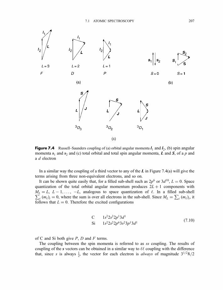
In a similar way the coupling of a third vector to any of the L in Figure 7.4(a) will give the
terms arising from three non-equivalent electrons, and so on.
It can be shown quite easily that, for a filled sub-shell such as 2p6 or 3d10, L ¼ 0. Space
quantization of the total orbital angular momentum produces 2Lþ 1 components with
ML ¼ L, L� 1; . . . , �L, analogous to space quantization of ‘. In a filled sub-shellPi ðm‘Þi ¼ 0, where the sum is over all electrons in the sub-shell. Since ML ¼
Pi ðm‘Þi, it
follows that L ¼ 0. Therefore the excited configurations
C
Si
1s22s22p13d1
1s22s22p63s23p13d1ð7:10Þ
of C and Si both give P, D and F terms.
The coupling between the spin momenta is referred to as ss coupling. The results of
coupling of the s vectors can be obtained in a similar way to ‘‘ coupling with the difference
that, since s is always 12, the vector for each electron is always of magnitude 31=2"=2
Figure 7.4 Russell–Saunders coupling of (a) orbital angular momenta l1 and l2, (b) spin angular
momenta s1 and s2 and (c) total orbital and total spin angular momenta, L and S, of a p and
a d electron
7.1 ATOMIC SPECTROSCOPY 207
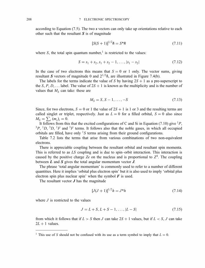
according to Equation (7.5). The two s vectors can only take up orientations relative to each
other such that the resultant S is of magnitude
½SðS þ 1Þ�1=2h ¼ S*h ð7:11Þ
where S, the total spin quantum number,1 is restricted to the values:
S ¼ s1 þ s2; s1 þ s2 � 1; . . . ; js1 � s2j ð7:12Þ
In the case of two electrons this means that S ¼ 0 or 1 only. The vector sums, giving
resultant S vectors of magnitude 0 and 21=2", are illustrated in Figure 7.4(b).
The labels for the terms indicate the value of S by having 2S þ 1 as a pre-superscript to
the S, P, D, . . . label. The value of 2S þ 1 is known as the multiplicity and is the number of
values that MS can take: these are
MS ¼ S; S � 1; . . . ;�S ð7:13Þ
Since, for two electrons, S ¼ 0 or 1 the value of 2S þ 1 is 1 or 3 and the resulting terms are
called singlet or triplet, respectively. Just as L ¼ 0 for a filled orbital, S ¼ 0 also since
MS ¼P
i ðmsÞi ¼ 0.
It follows from this that the excited configurations of C and Si in Equation (7.10) give 1P,3P, 1D, 3D, 1F and 3F terms. It follows also that the noble gases, in which all occupied
orbitals are filled, have only 1S terms arising from their ground configurations.
Table 7.2 lists the terms that arise from various combinations of two non-equivalent
electrons.
There is appreciable coupling between the resultant orbital and resultant spin momenta.
This is referred to as LS coupling and is due to spin–orbit interaction. This interaction is
caused by the positive charge Ze on the nucleus and is proportional to Z4. The coupling
between L and S gives the total angular momentum vector J.
The phrase ‘total angular momentum’ is commonly used to refer to a number of different
quantities. Here it implies ‘orbital plus electron spin’ but it is also used to imply ‘orbital plus
electron spin plus nuclear spin’ when the symbol F is used.
The resultant vector J has the magnitude
½J ðJ þ 1Þ�1=2h ¼ J*h ð7:14Þ
where J is restricted to the values
J ¼ Lþ S; Lþ S � 1; . . . ; jL� Sj ð7:15Þ
from which it follows that if L > S then J can take 2S þ 1 values, but if L < S, J can take
2Lþ 1 values.
1 This use of S should not be confused with its use as a term symbol to imply that L ¼ 0.
208 7 ELECTRONIC SPECTROSCOPY
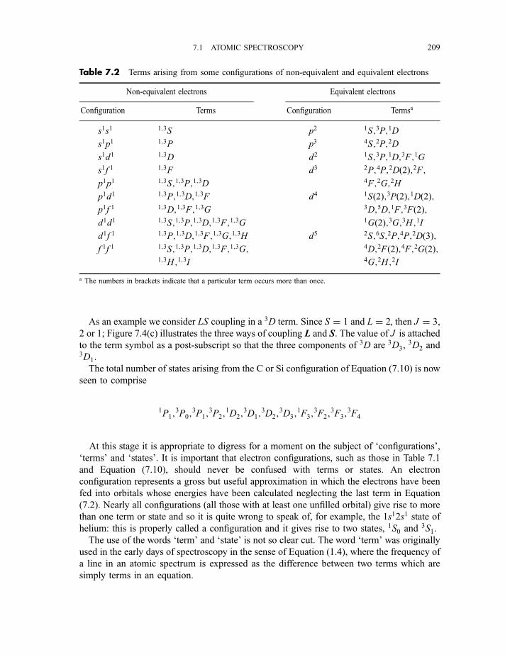
As an example we consider LS coupling in a 3D term. Since S ¼ 1 and L ¼ 2, then J ¼ 3,
2 or 1; Figure 7.4(c) illustrates the three ways of coupling L and S. The value of J is attached
to the term symbol as a post-subscript so that the three components of 3D are 3D3,3D2 and
3D1.
The total number of states arising from the C or Si configuration of Equation (7.10) is now
seen to comprise
1P1;3P0;
3P1;3P2;
1D2;3D1;
3D2;3D3;
1F3;3F2;
3F3;3F4
At this stage it is appropriate to digress for a moment on the subject of ‘configurations’,
‘terms’ and ‘states’. It is important that electron configurations, such as those in Table 7.1
and Equation (7.10), should never be confused with terms or states. An electron
configuration represents a gross but useful approximation in which the electrons have been
fed into orbitals whose energies have been calculated neglecting the last term in Equation
(7.2). Nearly all configurations (all those with at least one unfilled orbital) give rise to more
than one term or state and so it is quite wrong to speak of, for example, the 1s12s1 state of
helium: this is properly called a configuration and it gives rise to two states, 1S0 and 3S1.
The use of the words ‘term’ and ‘state’ is not so clear cut. The word ‘term’ was originally
used in the early days of spectroscopy in the sense of Equation (1.4), where the frequency of
a line in an atomic spectrum is expressed as the difference between two terms which are
simply terms in an equation.
Table 7.2 Terms arising from some configurations of non-equivalent and equivalent electrons
Non-equivalent electrons Equivalent electrons
Configuration Terms Configuration Termsa
s1s1 1;3S p2 1S;3P;1D
s1p1 1;3P p3 4S;2P;2D
s1d1 1;3D d2 1S;3P;1D;3F;1G
s1f 1 1;3F d3 2P;4P;2Dð2Þ;2F;p1p1 1;3S;1;3P;1;3D 4F;2G;2H
p1d1 1;3P;1;3D;1;3F d4 1Sð2Þ;3Pð2Þ;1Dð2Þ;p1f 1 1;3D;1;3F;1;3G 3D;5D;1F;3Fð2Þ;d1d1 1;3S;1;3P;1;3D;1;3F;1;3G 1Gð2Þ;3G;3H;1I
d1f 1 1;3P;1;3D;1;3F;1;3G;1;3H d5 2S;6S;2P;4P;2Dð3Þ;f 1f 1 1;3S;1;3P;1;3D;1;3F;1;3G; 4D;2Fð2Þ;4F;2Gð2Þ;
1;3H;1;3I 4G;2H;2I
a The numbers in brackets indicate that a particular term occurs more than once.
7.1 ATOMIC SPECTROSCOPY 209
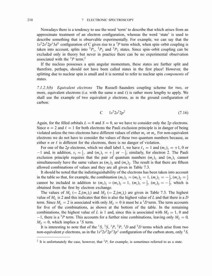
Nowadays there is a tendency to use the word ‘term’ to describe that which arises from an
approximate treatment of an electron configuration, whereas the word ‘state’ is used to
describe something that is observable experimentally. For example, we can say that the
1s22s22p13d1 configuration of C gives rise to a 3P term which, when spin–orbit coupling is
taken into account, splits into 3P1,3P2 and 3P3 states. Since spin–orbit coupling can be
excluded only in theory but never in practice there can be no experimental observation
associated with the 3P term.2
If the nucleus possesses a spin angular momentum, these states are further split and
therefore, perhaps, should not have been called states in the first place! However, the
splitting due to nuclear spin is small and it is normal to refer to nuclear spin components of
states.
7.1.2.3(b) Equivalent electrons The Russell–Saunders coupling scheme for two, or
more, equivalent electrons (i.e. with the same n and ‘) is rather more lengthy to apply. We
shall use the example of two equivalent p electrons, as in the ground configuration of
carbon:
C 1s22s22p2 ð7:16Þ
Again, for the filled orbitals L ¼ 0 and S ¼ 0, so we have to consider only the 2p electrons.
Since n ¼ 2 and ‘ ¼ 1 for both electrons the Pauli exclusion principle is in danger of being
violated unless the two electrons have different values of either m‘ or ms. For non-equivalent
electrons we do not have to consider the values of these two quantum numbers because, as
either n or ‘ is different for the electrons, there is no danger of violation.
For one of the 2p electrons, which we shall label 1, we have ‘1 ¼ 1 and ðm‘Þ1 ¼ þ1, 0 or
�1 and, in addition, s1 ¼ 12; and ðmsÞ1 ¼ þ 1
2or � 1
2; similarly, for electron 2. The Pauli
exclusion principle requires that the pair of quantum numbers ðm‘Þ1 and ðmsÞ1 cannot
simultaneously have the same values as ðm‘Þ2 and ðmsÞ2. The result is that there are fifteen
allowed combinations of values and they are all given in Table 7.3.
It should be noted that the indistinguishability of the electrons has been taken into account
in the table so that, for example, the combination ðm‘Þ1 ¼ ðm‘Þ2 ¼ 1, ðmsÞ1 ¼ � 12, ðmsÞ2 ¼ 1
2
cannot be included in addition to ðm‘Þ1 ¼ ðm‘Þ2 ¼ 1, ðmsÞ1 ¼ 12, ðmsÞ2 ¼ � 1
2, which is
obtained from the first by electron exchange.
The values of ML ð¼ Siðm‘ÞiÞ and MS ð¼ SiðmsÞiÞ are given in Table 7.3. The highest
value ofML is 2 and this indicates that this is also the highest value of L and that there is a D
term. Since ML ¼ 2 is associated with only MS ¼ 0 it must be a 1D term. The term accounts
for five of the combinations, as shown at the bottom of the table. In the remaining
combinations, the highest value of L is 1 and, since this is associated with MS ¼ 1, 0 and
�1, there is a 3P term. This accounts for a further nine combinations, leaving only ML ¼ 0,
MS ¼ 0, which implies a 1S term.
It is interesting to note that of the 1S, 3S, 1P, 3P, 1D and 3D terms which arise from two
non-equivalent p electrons, as in the 1s22s22p13p1 configuration of the carbon atom, only 1S,
2 It is unfortunately the case, however, that 3P, for example, is sometimes referred to as a state.
210 7 ELECTRONIC SPECTROSCOPY
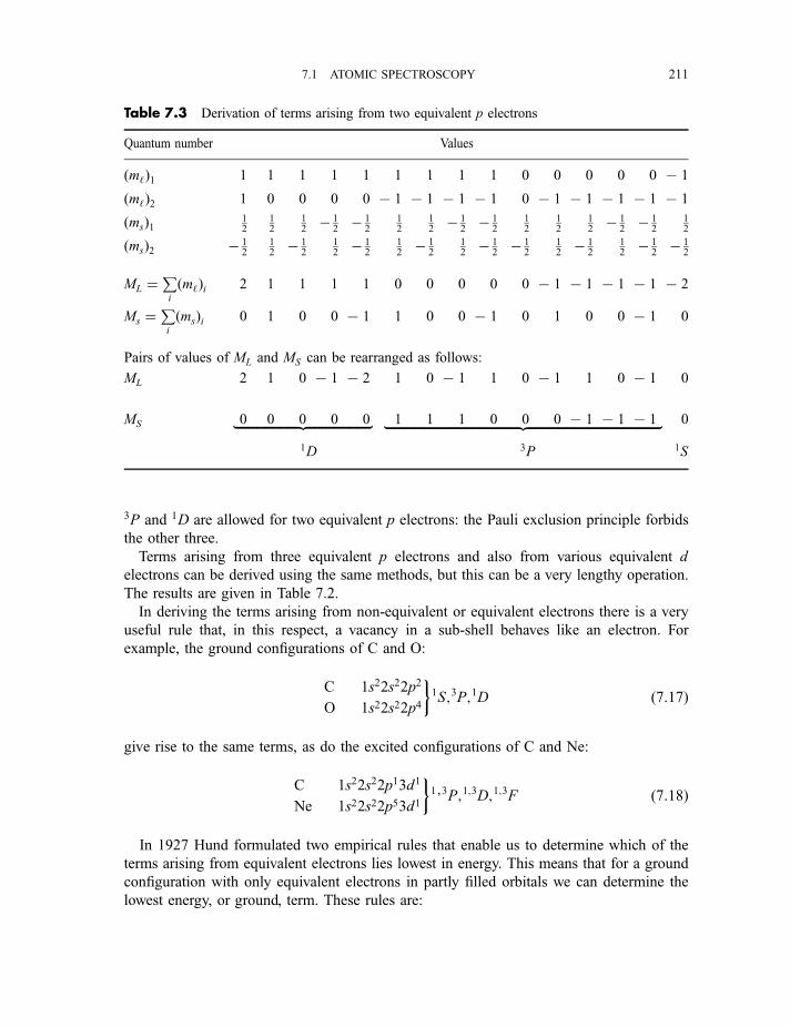
3P and 1D are allowed for two equivalent p electrons: the Pauli exclusion principle forbids
the other three.
Terms arising from three equivalent p electrons and also from various equivalent d
electrons can be derived using the same methods, but this can be a very lengthy operation.
The results are given in Table 7.2.
In deriving the terms arising from non-equivalent or equivalent electrons there is a very
useful rule that, in this respect, a vacancy in a sub-shell behaves like an electron. For
example, the ground configurations of C and O:
C
O
1s22s22p2
1s22s22p4
�1S;3P;1D ð7:17Þ
give rise to the same terms, as do the excited configurations of C and Ne:
C
Ne
1s22s22p13d1
1s22s22p53d1
�1;3P;1;3D;1;3F ð7:18Þ
In 1927 Hund formulated two empirical rules that enable us to determine which of the
terms arising from equivalent electrons lies lowest in energy. This means that for a ground
configuration with only equivalent electrons in partly filled orbitals we can determine the
lowest energy, or ground, term. These rules are:
Table 7.3 Derivation of terms arising from two equivalent p electrons
Quantum number Values
ðm‘Þ1 1 1 1 1 1 1 1 1 1 0 0 0 0 0 7 1
ðm‘Þ2 1 0 0 0 0 7 1 7 1 7 1 7 1 0 7 1 7 1 7 1 7 1 7 1
ðmsÞ1 12
12
12� 1
2� 1
212
12� 1
2� 1
212
12
12� 1
2� 1
212
ðmsÞ2 � 12
12� 1
212� 1
212� 1
212� 1
2� 1
212� 1
212� 1
2� 1
2
ML ¼Pi
ðm‘Þi 2 1 1 1 1 0 0 0 0 0 7 1 7 1 7 1 7 1 7 2
Ms ¼Pi
ðmsÞi 0 1 0 0 7 1 1 0 0 7 1 0 1 0 0 7 1 0
Pairs of values of ML and MS can be rearranged as follows:
ML 2 1 0 7 1 7 2 1 0 7 1 1 0 7 1 1 0 7 1 0
MS 0 0 0 0 0 1 1 1 0 0 0 7 1 7 1 7 1 0
1D 3P 1S
8 > > > > > > > > > > > > < > > > > > > > > > > > > : 8 > > > > > > > > > > > > > > > > > > > > > > > > > > > > > > < > > > > > > > > > > > > > > > > > > > > > > > > > > > > > > :
7.1 ATOMIC SPECTROSCOPY 211
1. Of the terms arising from equivalent electrons those with the highest multiplicity lie
lowest in energy.
2. Of these, the lowest is that with the highest value of L.
Using these rules it follows that, for the ground configurations of both C and O in
Equation (7.17), the 3P term is the lowest in energy.
The ground configuration of Ti is
Ti KL3s23p63d24s2 ð7:19Þ
Of the terms arising from the d2 configuration given in Table 7.2 the rules indicate that 3F
is the lowest in energy.
The splitting of a term by spin–orbit interaction is proportional to J:
EJ � EJ�1 ¼ AJ ð7:20Þ
where EJ is the energy corresponding to J , and a multiplet results. If A is positive, the
component with the smallest value of J lies lowest in energy and the multiplet is said to be
normal whereas if A is negative the multiplet is inverted.
There are two further rules for ground terms which tell us whether a multiplet arising from
equivalent electrons is normal or inverted.
3. Normal multiplets arise from equivalent electrons when a partially filled orbital is less
than half full.
4. Inverted multiplets arise from equivalent electrons when a partially filled orbital is more
than half full.
It follows that the lowest energy term of Ti, 3F, is split by spin–orbit coupling into a
normal multiplet and therefore the ground state is 3F2. Similarly, the lowest energy term of
C, 3P, splits into a normal multiplet resulting in a 3P0 ground state, whereas that of O, with
an inverted multiplet, is 3P2.
Atoms with a ground configuration in which an orbital is exactly half-filled, as for
example in Nð2p3Þ, Mnð3d5Þ and Euð4f 7Þ, always have an S ground state. Since such states
have only one component the problem of a normal or inverted multiplet does not arise. Table
7.1 gives the ground states of all atoms in the periodic table.
For excited terms split by spin–orbit interaction there are no general rules regarding
normal or inverted multiplets. For example, in He, excited states form mostly inverted
multiplets whereas in the alkaline earth metals, Be, Mg, Ca, . . . , they are mostly normal.
There is one further addition to the state symbolism that we have not mentioned so far.
This is the superscript ‘o’ as in the ground state of boron, 2Po1=2. The symbol implies that the
arithmetic sum Si‘i for all the electrons in the atoms is an odd number, 1 in this case. When
there is no such superscript this implies that the sum is an even number; for example it is 4 in
the case of oxygen.
212 7 ELECTRONIC SPECTROSCOPY
7.1.3 Spectra of alkali metal atoms
The hydrogen atom and one-electron ions are the simplest systems in the sense that, having
only one electron, there are no inter-electron repulsions. However, this unique property leads
to degeneracies, or near-degeneracies, which are absent in all other atoms and ions. The
result is that the spectrum of the hydrogen atom, although very simple in its coarse structure
(Figure 1.1) is more unusual in its fine structure than those of polyelectronic atoms. For this
reason we shall defer a discussion of its spectrum to the next section.
The alkali metal atoms all have one valence electron in an outer ns orbital, where n ¼ 2, 3,
4, 5, 6 for Li, Na, K, Rb and Cs. If we consider only orbital changes involving this electron
the behaviour is expected to resemble that of the hydrogen atom. The reason for this is that
the core, consisting of the nucleus of charge þZe and filled orbitals containing ðZ � 1Þelectrons, has a net charge of þe and therefore has an effect on the valence electron which issimilar to that of the nucleus of the hydrogen atom on its electron.
Whereas the emission spectrum of the hydrogen atom shows only one series, the Balmer
series (see Figure 1.1), in the visible region the alkali metals show at least three. The spectra
can be excited in a discharge lamp containing a sample of the appropriate metal. One series
was called the principal series because it could also be observed in absorption through a
column of the vapour. The other two were called sharp and diffuse because of their general
appearance. A part of a fourth series, called the fundamental series, can sometimes be
observed.
Figure 7.5 shows these series schematically for lithium. All such series converge smoothly
towards high energy (low wavelength) in a way that resembles the series in the hydrogen
spectrum.
Figure 7.6 shows an energy level diagram, a so-called Grotrian diagram, for lithium for
which the ground configuration is 1s22s1. The lowest energy level corresponds to this
configuration. The higher energy levels are labelled according to the orbital to which the
valence electron has been promoted: for example the level labelled 4p corresponds to the
configuration 1s24p1.
The relatively large energy separation between configurations in which the valence
electron is in orbitals differing only in the value of ‘ (e.g. 1s23s1, 1s23p1, 1s23d1) is
characteristic of all atoms except hydrogen (and one-electron ions).
The selection rules governing the promotion of the electron to an excited orbital, and also
its falling back from an excited orbital, are
ðaÞðbÞ
Dn is unrestricted
D‘ ¼ �1�
ð7:21Þ
These selection rules lead to the sharp, principal, diffuse and fundamental series, shown in
Figures 7.5 and 7.6, in which the promoted electron is in an s, p, d and f orbital,
respectively. Indeed, these rather curious orbital symbols originate from the first letters of the
corresponding series observed in the spectrum.
7.1 ATOMIC SPECTROSCOPY 213
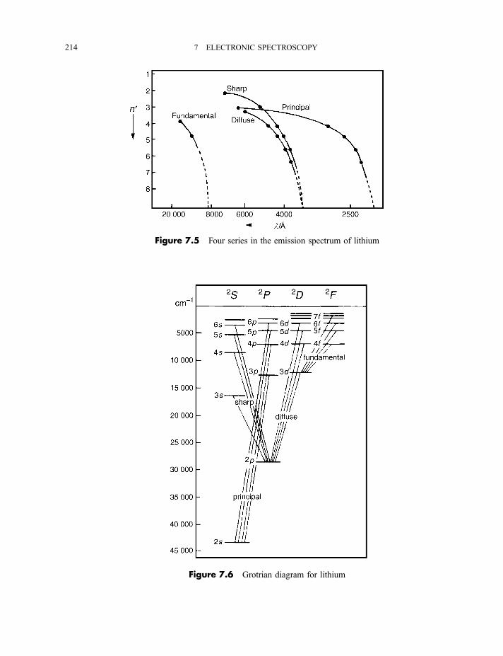
Figure 7.6 Grotrian diagram for lithium
Figure 7.5 Four series in the emission spectrum of lithium
214 7 ELECTRONIC SPECTROSCOPY
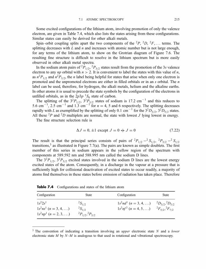
Some excited configurations of the lithium atom, involving promotion of only the valence
electron, are given in Table 7.4, which also lists the states arising from these configurations.
Similar states can easily be derived for other alkali metals.
Spin–orbit coupling splits apart the two components of the 2P, 2D, 2F, . . . terms. The
splitting decreases with L and n and increases with atomic number but is not large enough,
for any terms of the lithium atom, to show on the Grotrian diagram of Figure 7.6. The
resulting fine structure is difficult to resolve in the lithium spectrum but is more easily
observed in other alkali metal spectra.
In the sodium atom pairs of 2P1=2,2P3=2 states result from the promotion of the 3s valence
electron to any np orbital with n > 2. It is convenient to label the states with this value of n,
as n2P1=2 and n2P3=2, the n label being helpful for states that arise when only one electron is
promoted and the unpromoted electrons are either in filled orbitals or in an s orbital. The n
label can be used, therefore, for hydrogen, the alkali metals, helium and the alkaline earths.
In other atoms it is usual to precede the state symbols by the configuration of the electrons in
unfilled orbitals, as in the 2p3p 1S0 state of carbon.
The splitting of the 32P1=2, 32P3=2 states of sodium is 17.2 cm71 and this reduces to
5.6 cm71, 2.5 cm71 and 1.3 cm71 for n ¼ 4, 5 and 6 respectively. The splitting decreases
rapidly with L as exemplified by the splitting of only 0.1 cm71 for the 32D3=2, 32D5=2 states.
All these 2P and 2D multiplets are normal, the state with lowest J lying lowest in energy.
The fine structure selection rule is
D J ¼ 0;�1 except J ¼ 0$j J ¼ 0 ð7:22Þ
The result is that the principal series consists of pairs of 2P1=2 �2 S1=2,2P3=2 �2 S1=2
transitions,3 as illustrated in Figure 7.7(a). The pairs are known as simple doublets. The first
member of this series in sodium appears in the yellow region of the spectrum with
components at 589.592 nm and 588.995 nm called the sodium D lines.
The 32P1=2, 32P3=2 excited states involved in the sodium D lines are the lowest energy
excited states of the atom. Consequently, in a discharge in the vapour at a pressure that is
sufficiently high for collisional deactivation of excited states to occur readily, a majority of
atoms find themselves in these states before emission of radiation has taken place. Therefore
3 The convention of indicating a transition involving an upper electronic state N and a lower
electronic state M by N–M is analogous to that used in rotational and vibrational spectroscopy.
Table 7.4 Configurations and states of the lithium atom
Configuration State Configuration State
1s22s1 2S1=2 1s2nd1 ðn ¼ 3; 4; . . .Þ 2D3=2;2D5=2
1s2ns1 ðn ¼ 3; 4; . . .Þ 2S1=2 1s2nf 2 ðn ¼ 4; 5; . . .Þ 2F5=2;2F7=2
1s2np1 ðn ¼ 2; 3; . . .Þ 2P1=2;2P3=2
7.1 ATOMIC SPECTROSCOPY 215
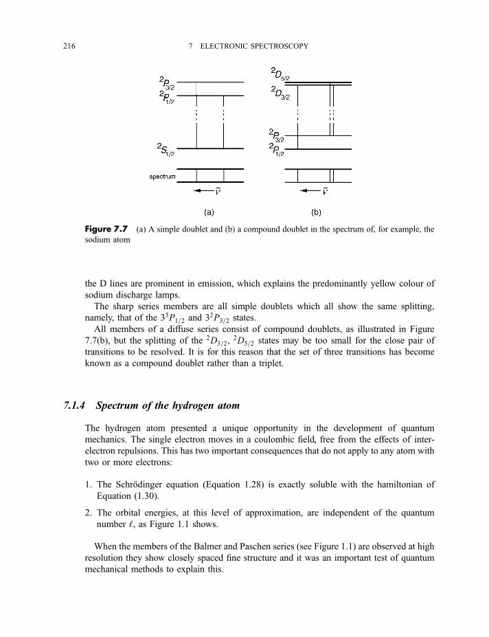
the D lines are prominent in emission, which explains the predominantly yellow colour of
sodium discharge lamps.
The sharp series members are all simple doublets which all show the same splitting,
namely, that of the 33P1=2 and 32P3=2 states.
All members of a diffuse series consist of compound doublets, as illustrated in Figure
7.7(b), but the splitting of the 2D3=2,2D5=2 states may be too small for the close pair of
transitions to be resolved. It is for this reason that the set of three transitions has become
known as a compound doublet rather than a triplet.
7.1.4 Spectrum of the hydrogen atom
The hydrogen atom presented a unique opportunity in the development of quantum
mechanics. The single electron moves in a coulombic field, free from the effects of inter-
electron repulsions. This has two important consequences that do not apply to any atom with
two or more electrons:
1. The Schrodinger equation (Equation 1.28) is exactly soluble with the hamiltonian of
Equation (1.30).
2. The orbital energies, at this level of approximation, are independent of the quantum
number ‘, as Figure 1.1 shows.
When the members of the Balmer and Paschen series (see Figure 1.1) are observed at high
resolution they show closely spaced fine structure and it was an important test of quantum
mechanical methods to explain this.
Figure 7.7 (a) A simple doublet and (b) a compound doublet in the spectrum of, for example, the
sodium atom
216 7 ELECTRONIC SPECTROSCOPY
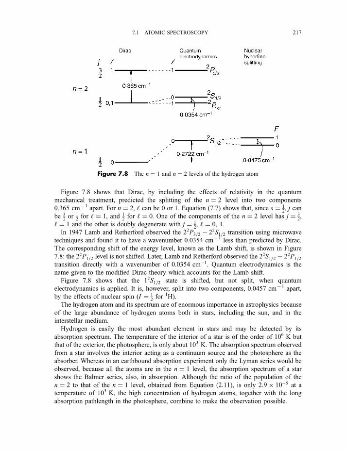
Figure 7.8 shows that Dirac, by including the effects of relativity in the quantum
mechanical treatment, predicted the splitting of the n ¼ 2 level into two components
0.365 cm71 apart. For n ¼ 2, ‘ can be 0 or 1. Equation (7.7) shows that, since s ¼ 12, j can
be 32or 1
2for ‘ ¼ 1, and 1
2for ‘ ¼ 0. One of the components of the n ¼ 2 level has j ¼ 3
2,
‘ ¼ 1 and the other is doubly degenerate with j ¼ 12, ‘ ¼ 0, 1.
In 1947 Lamb and Retherford observed the 22P3=2 � 22S1=2 transition using microwave
techniques and found it to have a wavenumber 0.0354 cm71 less than predicted by Dirac.
The corresponding shift of the energy level, known as the Lamb shift, is shown in Figure
7.8: the 22P1=2 level is not shifted. Later, Lamb and Retherford observed the 22S1=2 � 22P1=2
transition directly with a wavenumber of 0.0354 cm�1. Quantum electrodynamics is the
name given to the modified Dirac theory which accounts for the Lamb shift.
Figure 7.8 shows that the 12S1=2 state is shifted, but not split, when quantum
electrodynamics is applied. It is, however, split into two components, 0.0457 cm71 apart,
by the effects of nuclear spin (I ¼ 12for 1H).
The hydrogen atom and its spectrum are of enormous importance in astrophysics because
of the large abundance of hydrogen atoms both in stars, including the sun, and in the
interstellar medium.
Hydrogen is easily the most abundant element in stars and may be detected by its
absorption spectrum. The temperature of the interior of a star is of the order of 106 K but
that of the exterior, the photosphere, is only about 103 K. The absorption spectrum observed
from a star involves the interior acting as a continuum source and the photosphere as the
absorber. Whereas in an earthbound absorption experiment only the Lyman series would be
observed, because all the atoms are in the n ¼ 1 level, the absorption spectrum of a star
shows the Balmer series, also, in absorption. Although the ratio of the population of the
n ¼ 2 to that of the n ¼ 1 level, obtained from Equation (2.11), is only 2:9� 10�5 at a
temperature of 103 K, the high concentration of hydrogen atoms, together with the long
absorption pathlength in the photosphere, combine to make the observation possible.
Figure 7.8 The n ¼ 1 and n ¼ 2 levels of the hydrogen atom
7.1 ATOMIC SPECTROSCOPY 217
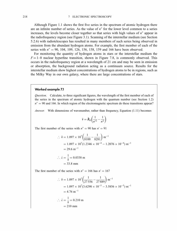
Although Figure 1.1 shows the first five series in the spectrum of atomic hydrogen there
are an infinite number of series. As the value of n00 for the lower level common to a series
increases, the levels become closer together so that series with high values of n00 appear inthe radiofrequency region (see Figure 3.1). Scanning of the interstellar medium (see Section
5.2.6) with radiotelescopes has resulted in many members of such series being observed in
emission from the abundant hydrogen atoms. For example, the first member of each of the
series with n00 ¼ 90, 104, 109, 126, 156, 158, 159 and 166 have been observed.
For monitoring the quantity of hydrogen atoms in stars or the interstellar medium the
F¼ 1–0 nuclear hyperfine transition, shown in Figure 7.8, is commonly observed. This
occurs in the radiofrequency region at a wavelength of 21 cm and may be seen in emission
or absorption, the background radiation acting as a continuum source. Results for the
interstellar medium show highest concentrations of hydrogen atoms to be in regions, such as
the Milky Way in our own galaxy, where there are large concentrations of stars.
Worked example 7.1
Question. Calculate, to three significant figures, the wavelength of the first member of each of
the series in the spectrum of atomic hydrogen with the quantum number (see Section 1.2)
n00 ¼ 90 and 166. In which region of the electromagnetic spectrum do these transitions appear?
Answer. With dimensions of wavenumber, rather than frequency, Equation (1.11) becomes
~nn ¼ ~RRH
1
n002� 1
n02
� �
The first member of the series with n00 ¼ 90 has n0 ¼ 91
; ~nn ¼ 1:097� 1071
8100� 1
8281
� �m�1
¼ 1:097� 107ð1:2346� 10�4 � 1:2076� 10�4Þ m�1¼ 29:6 m�1
; l ¼ 1
~nn¼ 0:0338 m
¼ 33:8 mm
The first member of the series with n00 ¼ 166 has n0 ¼ 167
; ~nn ¼ 1:097� 1071
27 556� 1
27 889
� �m�1
¼ 1:097� 107ð3:6290� 10�5 � 3:5856� 10�5Þ m�1¼ 4:76 m�1
; l ¼ 1
~nn¼ 0:210 m
¼ 210 mm
218 7 ELECTRONIC SPECTROSCOPY
Both the calculated wavelengths of 33.8 mm and 210 mm lie in the microwave region (see
Figure 3.1).
Note that five significant figures have been retained for the reciprocals of the squares of the
quantum numbers because, as you can see in the calculation, two of these figures are lost when
the reciprocals are subtracted.
7.1.5 Spectra of helium and the alkaline earth metal atoms
The emission spectrum of a discharge in helium gas in the visible and near-ultraviolet
regions appears rather like the spectrum of two alkali metals. It shows series of lines
converging smoothly to high energy (low wavelength) which can be divided into two groups.
One group consists of single lines and the other, at low resolution, double lines.
Derivation of an energy level diagram shows that it consists of two sets of energy levels,
one corresponding to the single lines and the other to the double lines, and that no transitions
between the two sets of levels are observed. For this reason it was suggested that helium
exists in two separate forms. In 1925 it became clear that, when account is taken of electron
spin, the two forms are really singlet helium and triplet helium.
For hydrogen and the alkali metal atoms in their ground configurations, or excited
configurations involving promotion of the valence electron, there is only one electron with
an unpaired spin. For this electron ms ¼ þ 12or � 1
2and the corresponding electron spin part
of the total wave function is conventionally given the symbol a or b. All states arising are
doublet states.
In helium we need to look more closely at the consequences of electron spin since this is
the prototype of all atoms and molecules having easily accessible states with two different
multiplicities.
If the spin–orbit coupling is small, as it is in helium, the total electronic wave function ce
can be factorized into an orbital part coe and a spin part cs
e:
ce ¼ coec
se ð7:23Þ
The spin part cse can be derived by labelling the electrons 1 and 2 and remembering that, in
general, each can have an a or b spin wave function giving four possible combinations:
að1Þbð2Þ, bð1Það2Þ, að1Það2Þ and bð1Þbð2Þ. Because the first two are neither symmetric nor
antisymmetric to the exchange of electrons, which is equivalent to the exchange of the labels
1 and 2, they must be replaced by linear combinations giving
cse ¼ 2�1=2½að1Þbð2Þ � bð1Það2Þ� ð7:24Þ
and
cse ¼ að1Það2Þor bð1Þbð2Þor 2�1=2½að1Þbð2Þ þ bð1Það2Þ� ð7:25Þ
7.1 ATOMIC SPECTROSCOPY 219
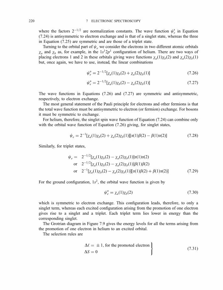
where the factors 2�1=2 are normalization constants. The wave function cse in Equation
(7.24) is antisymmetric to electron exchange and is that of a singlet state, whereas the three
in Equation (7.25) are symmetric and are those of a triplet state.
Turning to the orbital part of ce we consider the electrons in two different atomic orbitals
wa and wb as, for example, in the 1s12p1 configuration of helium. There are two ways of
placing electrons 1 and 2 in these orbitals giving wave functions wað1Þwbð2Þ and wað2Þwbð1Þbut, once again, we have to use, instead, the linear combinations
coe ¼ 2�1=2½wað1Þwbð2Þ þ wað2Þwbð1Þ� ð7:26Þ
coe ¼ 2�1=2½wað1Þwbð2Þ � wað2Þwbð1Þ� ð7:27Þ
The wave functions in Equations (7.26) and (7.27) are symmetric and antisymmetric,
respectively, to electron exchange.
The most general statement of the Pauli principle for electrons and other fermions is that
the total wave function must be antisymmetric to electron (or fermion) exchange. For bosons
it must be symmetric to exchange.
For helium, therefore, the singlet spin wave function of Equation (7.24) can combine only
with the orbital wave function of Equation (7.26) giving, for singlet states,
ce ¼ 2�1½wað1Þwbð2Þ þ wað2Þwbð1Þ�½að1Þbð2Þ � bð1Það2Þ� ð7:28Þ
Similarly, for triplet states,
ce ¼ 2�1=2½wað1Þwbð2Þ � wað2Þwbð1Þ�að1Það2Þor 2�1=2½wað1Þwbð2Þ � wað2Þwbð1Þ�bð1Þbð2Þor 2�1½wað1Þwbð2Þ � wað2Þwbð1Þ�½að1Þbð2Þ þ bð1Það2Þ� ð7:29Þ
For the ground configuration, 1s2, the orbital wave function is given by
coe ¼ wað1Þwbð2Þ ð7:30Þ
which is symmetric to electron exchange. This configuration leads, therefore, to only a
singlet term, whereas each excited configuration arising from the promotion of one electron
gives rise to a singlet and a triplet. Each triplet term lies lower in energy than the
corresponding singlet.
The Grotrian diagram in Figure 7.9 gives the energy levels for all the terms arising from
the promotion of one electron in helium to an excited orbital.
The selection rules are
D‘ ¼ � 1; for the promoted electron
DS ¼ 0
)ð7:31Þ
220 7 ELECTRONIC SPECTROSCOPY
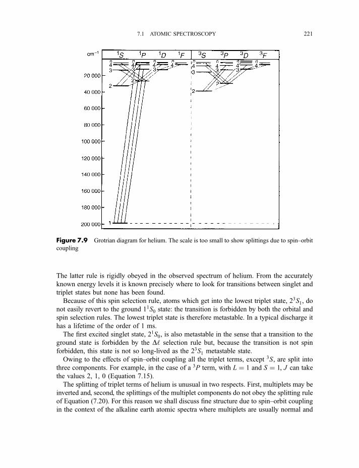
The latter rule is rigidly obeyed in the observed spectrum of helium. From the accurately
known energy levels it is known precisely where to look for transitions between singlet and
triplet states but none has been found.
Because of this spin selection rule, atoms which get into the lowest triplet state, 23S1, do
not easily revert to the ground 11S0 state: the transition is forbidden by both the orbital and
spin selection rules. The lowest triplet state is therefore metastable. In a typical discharge it
has a lifetime of the order of 1 ms.
The first excited singlet state, 21S0, is also metastable in the sense that a transition to the
ground state is forbidden by the D‘ selection rule but, because the transition is not spin
forbidden, this state is not so long-lived as the 23S1 metastable state.
Owing to the effects of spin–orbit coupling all the triplet terms, except 3S, are split into
three components. For example, in the case of a 3P term, with L ¼ 1 and S ¼ 1, J can take
the values 2, 1, 0 (Equation 7.15).
The splitting of triplet terms of helium is unusual in two respects. First, multiplets may be
inverted and, second, the splittings of the multiplet components do not obey the splitting rule
of Equation (7.20). For this reason we shall discuss fine structure due to spin–orbit coupling
in the context of the alkaline earth atomic spectra where multiplets are usually normal and
Figure 7.9 Grotrian diagram for helium. The scale is too small to show splittings due to spin–orbit
coupling
7.1 ATOMIC SPECTROSCOPY 221
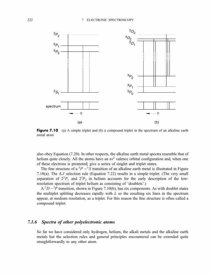
also obey Equation (7.20). In other respects, the alkaline earth metal spectra resemble that of
helium quite closely. All the atoms have an ns2 valence orbital configuration and, when one
of these electrons is promoted, give a series of singlet and triplet states.
The fine structure of a 3P �3S transition of an alkaline earth metal is illustrated in Figure
7.10(a). The D J selection rule (Equation 7.22) results in a simple triplet. (The very small
separation of 23P1 and 23P2 in helium accounts for the early description of the low-
resolution spectrum of triplet helium as consisting of ‘doublets’.)
A 3D�3P transition, shown in Figure 7.10(b), has six components. As with doublet states
the multiplet splitting decreases rapidly with L so the resulting six lines in the spectrum
appear, at medium resolution, as a triplet. For this reason the fine structure is often called a
compound triplet.
7.1.6 Spectra of other polyelectronic atoms
So far we have considered only hydrogen, helium, the alkali metals and the alkaline earth
metals but the selection rules and general principles encountered can be extended quite
straightforwardly to any other atom.
Figure 7.10 (a) A simple triplet and (b) a compound triplet in the spectrum of an alkaline earth
metal atom
222 7 ELECTRONIC SPECTROSCOPY
An obvious difference between the emission spectra of most atoms and those we have
considered so far is their complexity, the spectra showing very many lines and no obvious
series. An extreme example is the spectrum of iron, which is so rich in lines that it is
commonly used as a calibration spectrum throughout the visible and ultraviolet regions.
However complex the atom, we can use the Russell–Saunders coupling approximation (or
jj coupling, if necessary) to derive the states that arise from any configuration. The four
general selection rules that apply to transitions between these states are as follows.
Rule 1:
DL ¼ 0;�1 except L ¼ 0$j L ¼ 0 ð7:32Þ
Previously we have considered the promotion of only one electron, for which D‘ ¼ �1applies, but the general rule given here involves the total orbital angular momentum
quantum number L and applies to the promotion of any number of electrons.
Rule 2:
even$j even; odd$j odd; even$ odd ð7:33Þ
Here, ‘even’ and ‘odd’ refer to the arithmetic sum Si‘i over all the electrons and this
selection rule is called the Laporte rule. An important result of this is that transitions are
forbidden between states arising from the same configuration. For example, of the terms
given in Equation (7.18) arising from the 1s22s22p13d1 configuration of the carbon atom,
a 1P �1 D transition would be allowed if we considered only the DS (see Rule 4 below)
and DL selection rules, but the Laporte rule forbids it. Similarly, any transitions between
states arising from the 1s22s22p13d1 configuration, with Si‘i ¼ 3, and those arising from
the 1s22s23d14f 1 configuration, with Si‘i ¼ 5, are also forbidden.4 The Laporte rule is
consistent with D‘ ¼ �1 when only one electron is promoted from the ground
configuration.
Rule 3:
D J ¼ 0; �1 except J ¼ 0$j J ¼ 0 ð7:34Þ
This rule is the same for all atoms.
Rule 4:
DS ¼ 0 ð7:35Þ
4 The 22P3=2 � 22S1=2 and 22S1=2 � 22P1=2 transitions observed in the hydrogen atom violate the
Laporte rule because they are magnetic dipole transitions: the rule applies only to electric dipole
transitions.
7.1 ATOMIC SPECTROSCOPY 223
This applies only to atoms with a small nuclear charge. In atoms with a large nuclear
charge it breaks down so that the factorization of ce in Equation (7.23) no longer applies
because of spin–orbit interaction and states can no longer be described accurately as
singlet, doublet, etc. The mercury atom provides a good example of the breakdown of the
DS ¼ 0 selection rule. Having the ground configuration KLMN5s25p65d106s2 it is rather
like an alkaline earth metal. Promotion of an electron from the 6s to the 6p orbital
produces 61P1, 63P0, 6
3P1 and 63P2 states, the three components of 63P being widely
split by spin–orbit interaction. This interaction also breaks down the spin selection rule to
such an extent that the 63P1 � 61S0 transition at 253.652 nm is one of the strongest in the
mercury emission spectrum.
Worked example 7.2
Question. From the ground electron configuration of zirconium derive the ground state (i.e.
the values of L, S and J ) explaining which rules enable you to do this. Then derive the states
arising from the excited configuration
KLM4s24p64d15s25f 1
Assume that the Russell–Saunders coupling approximation applies to both configurations.
Answer. The ground electron configuration of zirconium ðZ ¼ 40Þ is (see Table 7.1)
KLM4s24p64d25s2
All filled orbitals contribute zero total orbital and total electron spin momenta. Therefore, in
deriving the states arising from the configuration we need consider only the two equivalent 4d
electrons. According to Table 7.2, the terms arising are
1S;3P;1D;3F and 1G
Hund’s rules tell us that the lowest energy term of these is 3F as it has the highest spin
multiplicity ð2S þ 1 ¼ 3Þ and the highest value of L (3 for an F term).
For the 3F term
J ¼ Lþ S;Lþ S � 1; . . . jL� Sj ¼ 4; 3; 2
giving three states
3F4;3F3 and
3F2
Since the unfilled orbital ð4dÞ is less than half full, the 3F multiplet is normal and the
component with the lowest value of J (i.e. 3F2) is the lowest in energy. Therefore the ground
state is 3F2.
In the excited electron configuration given, there are two electrons in partly filled orbitals, a
4d (electron 1) and a 5f electron (electron 2). These are non-equivalent electrons (Section
7.1.2.3a) and we need consider only the coupling of the orbital angular momenta, ‘1 and ‘2, and
the spin angular momenta, s1 and s2.
224 7 ELECTRONIC SPECTROSCOPY
For the coupling of the orbital angular momenta, ‘1 ¼ 2, ‘2 ¼ 3 and
L ¼ ‘1 þ ‘2; ‘1 þ ‘2 � 1; . . . j‘1 � ‘2j ¼ 5; 4; 3; 2; 1
giving H , G, F, D, P terms.
For coupling of the spin angular momenta, s1 ¼ 12, s2 ¼ 1
2and
S ¼ s1 þ s2; s1 þ s2 � 1; . . . js1 � s2j ¼ 1; 0
giving multiplicities ð2S þ 1Þ of 3 and 1.
The total number of terms is then
1H ;1G;1F;1D;1P;3H ;3G;3F;3D;3P
For each of the triplet terms there are three states. For example, for the 3H term, L ¼ 5, S ¼ 1
and
J ¼ Lþ S; Lþ S � 1; . . . jL� Sj ¼ 6; 5; 4
giving 3H6,3H5, and
3H4 states.
Similarly, we can show that the total number of states is
1H5;1G4;
1F3;1D2;
1P1;3H6;
3H5;3H4;
3G5;3G4;
3G3;3F4;
3F3;3F2;
3D3;3D2;
3D1;3P2;
3P1;3P0
There are 20 states(!) arising from this simple-looking d1f 1 configuration compared with only
nine
1G4;1D2;
1S0;3F4;
3F3;3F2;
3P2;3P1;
3P0
from the ground configuration.
When you consider the selection rules, which are not particularly restrictive (see Section
7.1.6), governing transitions between these states arising from each configuration, it is not
surprising that the electronic spectrum of an atom such as zirconium consists of very many
lines. (Remember that the Laporte rule of Equation (7.33) forbids transitions between states
arising from the same configuration.)
7.2 Electronic spectroscopy of diatomic molecules
7.2.1 Molecular orbitals
7.2.1.1 Homonuclear diatomic molecules
The molecular orbital (MO) approach to the electronic structure of diatomic, and also
polyatomic, molecules is not the only one which is used but it lends itself to a fairly
qualitative description, which we require here.
The approach adopted in the MO method is to consider the two nuclei, without their
electrons, a distance apart equal to the equilibrium internuclear distance and to construct
7.2 ELECTRONIC SPECTROSCOPY OF DIATOMIC MOLECULES 225
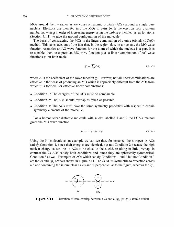
MOs around them – rather as we construct atomic orbitals (AOs) around a single bare
nucleus. Electrons are then fed into the MOs in pairs (with the electron spin quantum
number ms ¼ � 12) in order of increasing energy using the aufbau principle, just as for atoms
(Section 7.1.1), to give the ground configuration of the molecule.
The basis of constructing the MOs is the linear combination of atomic orbitals (LCAO)
method. This takes account of the fact that, in the region close to a nucleus, the MO wave
function resembles an AO wave function for the atom of which the nucleus is a part. It is
reasonable, then, to express an MO wave function c as a linear combination of AO wave
functions wi on both nuclei:
c ¼Pi
ciwi ð7:36Þ
where ci is the coefficient of the wave function wi. However, not all linear combinations are
effective in the sense of producing an MO which is appreciably different from the AOs from
which it is formed. For effective linear combinations:
Condition 1: The energies of the AOs must be comparable.
Condition 2: The AOs should overlap as much as possible.
Condition 3: The AOs must have the same symmetry properties with respect to certain
symmetry elements of the molecule.
For a homonuclear diatomic molecule with nuclei labelled 1 and 2 the LCAO method
gives the MO wave function
c ¼ c1w1 þ c2w2 ð7:37Þ
Using the N2 molecule as an example we can see that, for instance, the nitrogen 1s AOs
satisfy Condition 1, since their energies are identical, but not Condition 2 because the high
nuclear charge causes the 1s AOs to be close to the nuclei, resulting in little overlap. In
contrast the 2s AOs satisfy both conditions and, since they are spherically symmetrical,
Condition 3 as well. Examples of AOs which satisfy Conditions 1 and 2 but not Condition 3
are the 2s and 2px orbitals shown in Figure 7.11. The 2s AO is symmetric to reflection across
a plane containing the internuclear z axis and is perpendicular to the figure, whereas the 2px
Figure 7.11 Illustration of zero overlap between a 2s and a 2px (or 2py) atomic orbital
226 7 ELECTRONIC SPECTROSCOPY
AO is antisymmetric to this reflection. In fact, we can easily see that any overlap between 2s
and the positive lobe of 2px is exactly cancelled by that involving the negative lobe.
Important properties of the MO are the energy E associated with it and the value of c1 and
c2 in Equation (7.37). They are obtained from the Schrodinger equation
Hc ¼ Ec ð7:38Þ
Multiplying both sides by c*, the complex conjugate of c obtained from it by replacing all
i (equal top�1Þ by �i, and integrating over all space gives
E ¼Ðc*Hc dtÐc*c dt
ð7:39Þ
E can be calculated only if c is known, so what is done is to make an intelligent guess at the
MO wave function, say cn , and calculate the corresponding value of the energy �EEn from
Equation (7.39). A second guess at c, say cm , gives a corresponding energy �EEm. The
variation principle states that if �EEm < �EEn then cm is closer than cn to the true MO wave
function. This applies to the ground state only. In this way the true ground state wave
function can be approached as closely as we choose but this is usually done by varying
parameters in the chosen wave function until they have their optimum values.
Combining Equations (7.37) and (7.39) and assuming that w1 and w2 are not complex
gives
�EE ¼Ð ðc21w1Hw1 þ c1c2w1Hw2 þ c1c2w2Hw1 þ c22w2Hw2Þ dtÐ ðc21w21 þ 2c1c2w1w2 þ c22w
22Þ dt
ð7:40Þ
If the AO wave functions are normalized
ðw21 dt ¼
ðw22 dt ¼ 1 ð7:41Þ
and, as H is a hermitian operator,
ðw1Hw2 dt ¼
ðw2Hw1 dt ¼ H12 ðsayÞ ð7:42Þ
The quantity
ðw1w2 dt ¼ S ð7:43Þ
7.2 ELECTRONIC SPECTROSCOPY OF DIATOMIC MOLECULES 227
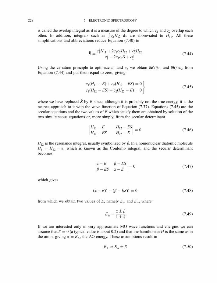
is called the overlap integral as it is a measure of the degree to which w1 and w2 overlap each
other. In addition, integrals such asÐw1Hw1 dt are abbreviated to H11. All these
simplifications and abbreviations reduce Equation (7.40) to
�EE ¼ c21H11 þ 2c1c2H12 þ c22H22
c21 þ 2c1c2S þ c22ð7:44Þ
Using the variation principle to optimize c1 and c2 we obtain @ �EE=@c1 and @ �EE=@c2 from
Equation (7.44) and put them equal to zero, giving
c1ðH11 � EÞ þ c2ðH12 � ESÞ ¼ 0
c1ðH12 � ESÞ þ c2ðH22 � EÞ ¼ 0
)ð7:45Þ
where we have replaced �EE by E since, although it is probably not the true energy, it is the
nearest approach to it with the wave function of Equation (7.37). Equations (7.45) are the
secular equations and the two values of E which satisfy them are obtained by solution of the
two simultaneous equations or, more simply, from the secular determinant
H11 � E
H12 � ES
H12 � ES
H22 � E
¼ 0 ð7:46Þ
H12 is the resonance integral, usually symbolized by b. In a homonuclear diatomic molecule
H11 ¼ H22 ¼ a, which is known as the Coulomb integral, and the secular determinant
becomes
a� E
b� ES
b� ES
a� E
¼ 0 ð7:47Þ
which gives
ða� EÞ2 � ðb� ESÞ2 ¼ 0 ð7:48Þ
from which we obtain two values of E, namely Eþ and E�, where
E� ¼a� b1� S
ð7:49Þ
If we are interested only in very approximate MO wave functions and energies we can
assume that S ¼ 0 (a typical value is about 0.2) and that the hamiltonian H is the same as in
the atom, giving a ¼ EA, the AO energy. These assumptions result in
E� ’ EA � b ð7:50Þ
228 7 ELECTRONIC SPECTROSCOPY
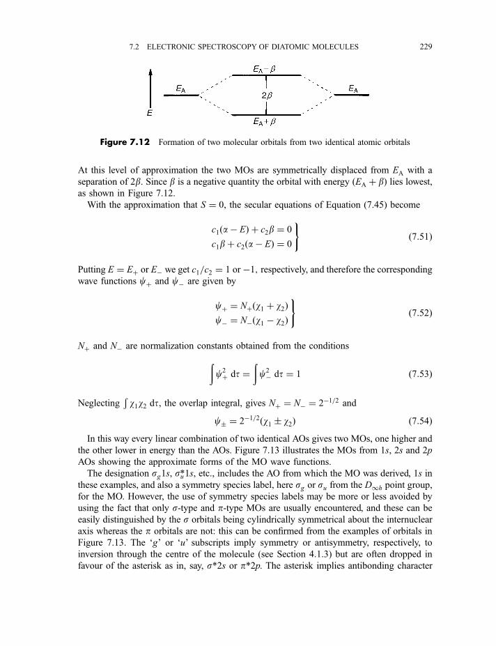
At this level of approximation the two MOs are symmetrically displaced from EA with a
separation of 2b. Since b is a negative quantity the orbital with energy ðEA þ bÞ lies lowest,as shown in Figure 7.12.
With the approximation that S ¼ 0, the secular equations of Equation (7.45) become
c1ða� EÞ þ c2b ¼ 0
c1bþ c2ða� EÞ ¼ 0
)ð7:51Þ
Putting E ¼ Eþ or E� we get c1=c2 ¼ 1 or �1; respectively, and therefore the correspondingwave functions cþ and c� are given by
cþ ¼ Nþðw1 þ w2Þc� ¼ N�ðw1 � w2Þ
)ð7:52Þ
Nþ and N� are normalization constants obtained from the conditionsðc2þ dt ¼
ðc2� dt ¼ 1 ð7:53Þ
NeglectingÐw1w2 dt, the overlap integral, gives Nþ ¼ N� ¼ 2�1=2 and
c� ¼ 2�1=2ðw1 � w2Þ ð7:54ÞIn this way every linear combination of two identical AOs gives two MOs, one higher and
the other lower in energy than the AOs. Figure 7.13 illustrates the MOs from 1s, 2s and 2p
AOs showing the approximate forms of the MO wave functions.
The designation sg1s, su*1s, etc., includes the AO from which the MO was derived, 1s in
these examples, and also a symmetry species label, here sg or su from the D1h point group,
for the MO. However, the use of symmetry species labels may be more or less avoided by
using the fact that only s-type and p-type MOs are usually encountered, and these can be
easily distinguished by the s orbitals being cylindrically symmetrical about the internuclear
axis whereas the p orbitals are not: this can be confirmed from the examples of orbitals in
Figure 7.13. The ‘g’ or ‘u’ subscripts imply symmetry or antisymmetry, respectively, to
inversion through the centre of the molecule (see Section 4.1.3) but are often dropped in
favour of the asterisk as in, say, s*2s or p*2p. The asterisk implies antibonding character
Figure 7.12 Formation of two molecular orbitals from two identical atomic orbitals
7.2 ELECTRONIC SPECTROSCOPY OF DIATOMIC MOLECULES 229
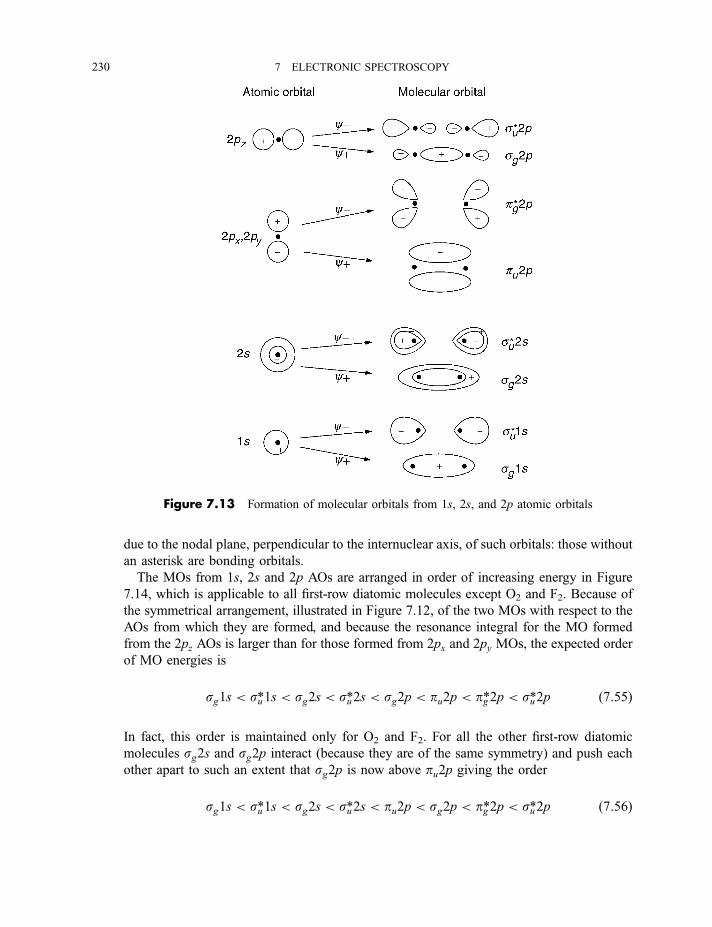
due to the nodal plane, perpendicular to the internuclear axis, of such orbitals: those without
an asterisk are bonding orbitals.
The MOs from 1s, 2s and 2p AOs are arranged in order of increasing energy in Figure
7.14, which is applicable to all first-row diatomic molecules except O2 and F2. Because of
the symmetrical arrangement, illustrated in Figure 7.12, of the two MOs with respect to the
AOs from which they are formed, and because the resonance integral for the MO formed
from the 2pz AOs is larger than for those formed from 2px and 2py MOs, the expected order
of MO energies is
sg1s < su*1s < sg2s < su*2s < sg2p < pu2p < pg*2p < su*2p ð7:55Þ
In fact, this order is maintained only for O2 and F2. For all the other first-row diatomic
molecules sg2s and sg2p interact (because they are of the same symmetry) and push each
other apart to such an extent that sg2p is now above pu2p giving the order
sg1s < su*1s < sg2s < su*2s < pu2p < sg2p < pg*2p < su*2p ð7:56Þ
Figure 7.13 Formation of molecular orbitals from 1s, 2s, and 2p atomic orbitals
230 7 ELECTRONIC SPECTROSCOPY
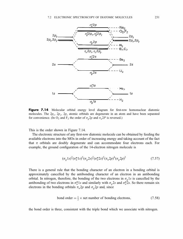
This is the order shown in Figure 7.14.
The electronic structure of any first-row diatomic molecule can be obtained by feeding the
available electrons into the MOs in order of increasing energy and taking account of the fact
that p orbitals are doubly degenerate and can accommodate four electrons each. For
example, the ground configuration of the 14-electron nitrogen molecule is
ðsg1sÞ2ðsu*1sÞ2ðsg2sÞ2ðsu*2sÞ2ðpu2pÞ4ðsg2pÞ2 ð7:57Þ
There is a general rule that the bonding character of an electron in a bonding orbital is
approximately cancelled by the antibonding character of an electron in an antibonding
orbital. In nitrogen, therefore, the bonding of the two electrons in sg1s is cancelled by the
antibonding of two electrons in su*1s and similarly with sg2s and su*2s. So there remain six
electrons in the bonding orbitals pu2p and sg2p and, since
bond order ¼ 12� net number of bonding electrons; ð7:58Þ
the bond order is three, consistent with the triple bond which we associate with nitrogen.
Figure 7.14 Molecular orbital energy level diagram for first-row homonuclear diatomic
molecules. The 2px, 2py, 2pz atomic orbitals are degenerate in an atom and have been separated
for convenience. (In O2 and F2 the order of sg2p and pu2P is reversed.)
7.2 ELECTRONIC SPECTROSCOPY OF DIATOMIC MOLECULES 231
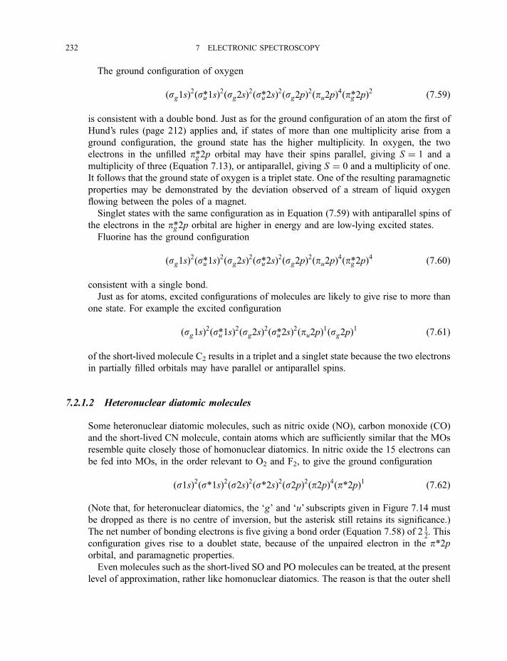
The ground configuration of oxygen
ðsg1sÞ2ðsu*1sÞ2ðsg2sÞ2ðsu*2sÞ2ðsg2pÞ2ðpu2pÞ4ðpg*2pÞ2 ð7:59Þ
is consistent with a double bond. Just as for the ground configuration of an atom the first of
Hund’s rules (page 212) applies and, if states of more than one multiplicity arise from a
ground configuration, the ground state has the higher multiplicity. In oxygen, the two
electrons in the unfilled pg*2p orbital may have their spins parallel, giving S ¼ 1 and a
multiplicity of three (Equation 7.13), or antiparallel, giving S ¼ 0 and a multiplicity of one.
It follows that the ground state of oxygen is a triplet state. One of the resulting paramagnetic
properties may be demonstrated by the deviation observed of a stream of liquid oxygen
flowing between the poles of a magnet.
Singlet states with the same configuration as in Equation (7.59) with antiparallel spins of
the electrons in the pg*2p orbital are higher in energy and are low-lying excited states.
Fluorine has the ground configuration
ðsg1sÞ2ðsu*1sÞ2ðsg2sÞ2ðsu*2sÞ2ðsg2pÞ2ðpu2pÞ4ðpg*2pÞ4 ð7:60Þ
consistent with a single bond.
Just as for atoms, excited configurations of molecules are likely to give rise to more than
one state. For example the excited configuration
ðsg1sÞ2ðsu*1sÞ2ðsg2sÞ2ðsu*2sÞ2ðpu2pÞ1ðsg2pÞ1 ð7:61Þ
of the short-lived molecule C2 results in a triplet and a singlet state because the two electrons
in partially filled orbitals may have parallel or antiparallel spins.
7.2.1.2 Heteronuclear diatomic molecules
Some heteronuclear diatomic molecules, such as nitric oxide (NO), carbon monoxide (CO)
and the short-lived CN molecule, contain atoms which are sufficiently similar that the MOs
resemble quite closely those of homonuclear diatomics. In nitric oxide the 15 electrons can
be fed into MOs, in the order relevant to O2 and F2, to give the ground configuration
ðs1sÞ2ðs*1sÞ2ðs2sÞ2ðs*2sÞ2ðs2pÞ2ðp2pÞ4ðp*2pÞ1 ð7:62Þ
(Note that, for heteronuclear diatomics, the ‘g’ and ‘u’ subscripts given in Figure 7.14 must
be dropped as there is no centre of inversion, but the asterisk still retains its significance.)
The net number of bonding electrons is five giving a bond order (Equation 7.58) of 2 12. This
configuration gives rise to a doublet state, because of the unpaired electron in the p*2porbital, and paramagnetic properties.
Even molecules such as the short-lived SO and PO molecules can be treated, at the present
level of approximation, rather like homonuclear diatomics. The reason is that the outer shell
232 7 ELECTRONIC SPECTROSCOPY
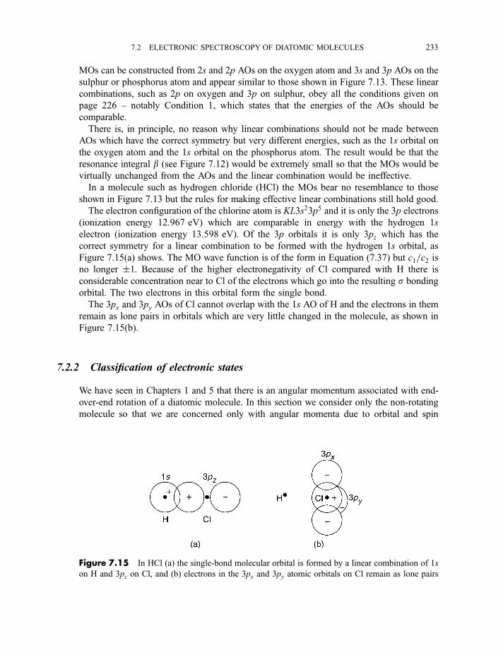
MOs can be constructed from 2s and 2p AOs on the oxygen atom and 3s and 3p AOs on the
sulphur or phosphorus atom and appear similar to those shown in Figure 7.13. These linear
combinations, such as 2p on oxygen and 3p on sulphur, obey all the conditions given on
page 226 – notably Condition 1, which states that the energies of the AOs should be
comparable.
There is, in principle, no reason why linear combinations should not be made between
AOs which have the correct symmetry but very different energies, such as the 1s orbital on
the oxygen atom and the 1s orbital on the phosphorus atom. The result would be that the
resonance integral b (see Figure 7.12) would be extremely small so that the MOs would be
virtually unchanged from the AOs and the linear combination would be ineffective.
In a molecule such as hydrogen chloride (HCl) the MOs bear no resemblance to those
shown in Figure 7.13 but the rules for making effective linear combinations still hold good.
The electron configuration of the chlorine atom is KL3s23p5 and it is only the 3p electrons
(ionization energy 12.967 eV) which are comparable in energy with the hydrogen 1s
electron (ionization energy 13.598 eV). Of the 3p orbitals it is only 3pz which has the
correct symmetry for a linear combination to be formed with the hydrogen 1s orbital, as
Figure 7.15(a) shows. The MO wave function is of the form in Equation (7.37) but c1=c2 isno longer �1. Because of the higher electronegativity of Cl compared with H there is
considerable concentration near to Cl of the electrons which go into the resulting s bonding
orbital. The two electrons in this orbital form the single bond.
The 3px and 3py AOs of Cl cannot overlap with the 1s AO of H and the electrons in them
remain as lone pairs in orbitals which are very little changed in the molecule, as shown in
Figure 7.15(b).
7.2.2 Classification of electronic states
We have seen in Chapters 1 and 5 that there is an angular momentum associated with end-
over-end rotation of a diatomic molecule. In this section we consider only the non-rotating
molecule so that we are concerned only with angular momenta due to orbital and spin
Figure 7.15 In HCl (a) the single-bond molecular orbital is formed by a linear combination of 1s
on H and 3pz on Cl, and (b) electrons in the 3px and 3py atomic orbitals on Cl remain as lone pairs
7.2 ELECTRONIC SPECTROSCOPY OF DIATOMIC MOLECULES 233
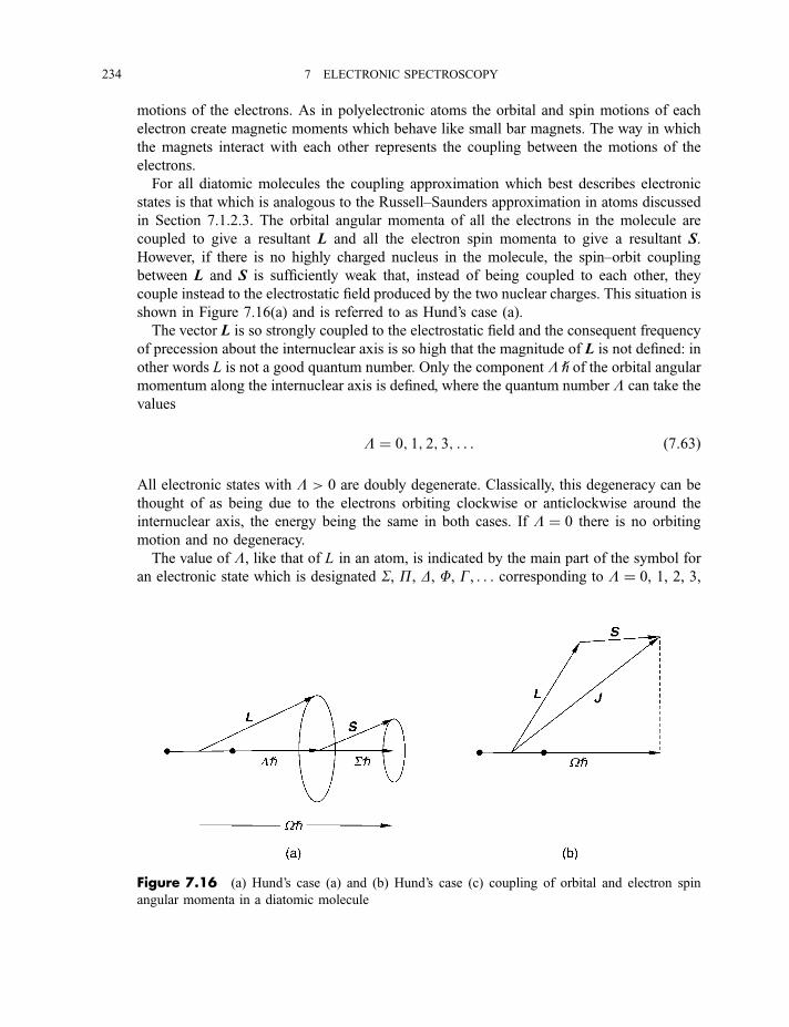
motions of the electrons. As in polyelectronic atoms the orbital and spin motions of each
electron create magnetic moments which behave like small bar magnets. The way in which
the magnets interact with each other represents the coupling between the motions of the
electrons.
For all diatomic molecules the coupling approximation which best describes electronic
states is that which is analogous to the Russell–Saunders approximation in atoms discussed
in Section 7.1.2.3. The orbital angular momenta of all the electrons in the molecule are
coupled to give a resultant L and all the electron spin momenta to give a resultant S.
However, if there is no highly charged nucleus in the molecule, the spin–orbit coupling
between L and S is sufficiently weak that, instead of being coupled to each other, they
couple instead to the electrostatic field produced by the two nuclear charges. This situation is
shown in Figure 7.16(a) and is referred to as Hund’s case (a).
The vector L is so strongly coupled to the electrostatic field and the consequent frequency
of precession about the internuclear axis is so high that the magnitude of L is not defined: in
other words L is not a good quantum number. Only the component L h of the orbital angular
momentum along the internuclear axis is defined, where the quantum number L can take the
values
L ¼ 0; 1; 2; 3; . . . ð7:63Þ
All electronic states with L > 0 are doubly degenerate. Classically, this degeneracy can be
thought of as being due to the electrons orbiting clockwise or anticlockwise around the
internuclear axis, the energy being the same in both cases. If L ¼ 0 there is no orbiting
motion and no degeneracy.
The value of L, like that of L in an atom, is indicated by the main part of the symbol for
an electronic state which is designated S, P, D, F, G, . . . corresponding to L ¼ 0, 1, 2, 3,
Figure 7.16 (a) Hund’s case (a) and (b) Hund’s case (c) coupling of orbital and electron spin
angular momenta in a diatomic molecule
234 7 ELECTRONIC SPECTROSCOPY
4, . . . . The letters S, P, D, F, G, . . . are the Greek equivalents of S, P, D, F, G, . . . used for
atoms.
The coupling of S to the internuclear axis is caused not by the electrostatic field, which
has no effect on it, but by the magnetic field along the axis due to the orbital motion of the
electrons. Figure 7.16(a) shows that the component of S along the internuclear axis is Sh.The quantum number S is analogous to MS in an atom and can take the values
S ¼ S; S � 1; . . . ;�S ð7:64Þ
S remains a good quantum number and, for states with L > 0, there are 2S þ 1 components
corresponding to the number of values that S can take. The multiplicity of the state is the
value of 2S þ 1 and is indicated, as in atoms, by a pre-superscript as, for example, in 3P.
The component of the total (orbital plus electron spin) angular momentum along the
internuclear axis is O h, shown in Figure 7.16(a), where the quantum number O is given by
O ¼ jLþ Sj ð7:65Þ
Since L ¼ 1 and S ¼ 1, 0, �1 the three components of 3P have O ¼ 2, 1, 0 and are
symbolized by 3P2,3P1, and
3P0:5
Spin–orbit interaction splits the components so that the energy level after interaction is
shifted by
DE ¼ ALS ð7:66Þ
where A is the spin–orbit coupling constant. The splitting produces what is called a normal
multiplet if the component with the lowest O has the lowest energy (i.e. A positive) and an
inverted multiplet if the component with the lowest O has the highest energy (i.e. A
negative).
For S states there is no orbital angular momentum and therefore no resulting magnetic
field to couple S to the internuclear axis. The result is that a S state has only one component,
whatever the multiplicity.
Hund’s case (a), shown in Figure 7.16(a), is the most commonly encountered case but, like
all assumed coupling of angular momenta, it is an approximation. However, when there is at
least one highly charged nucleus in the molecule, spin–orbit coupling may be sufficiently
large that L and S are not uncoupled by the electrostatic field of the nuclei. Instead, as shown
in Figure 7.16(b), L and S couple to give J, as in an atom, and J couples to the internuclear
axis along which the component is O h. This coupling approximation is known as Hund’s
case (c), in which L is no longer a good quantum number. The main label for a state is now
the value of O. This approximation is by no means as useful as Hund’s case (a) and, even
when it is used, states are often labelled with the value that L would have if it were a good
quantum number.
5 It is not important in this example but, in general, the value of the post-subscript is Lþ S not
jLþ Sj.
7.2 ELECTRONIC SPECTROSCOPY OF DIATOMIC MOLECULES 235
For atoms, electronic states may be classified and selection rules specified entirely by use
of the quantum numbers L, S and J . In diatomic molecules the quantum numbers L, S and Oare not quite sufficient. We must also use one (for heteronuclear) or two (for homonuclear)
symmetry properties of the electronic wave function ce.
The first is the ‘g’ or ‘u’ symmetry property which indicates that ce is symmetric or
antisymmetric respectively to inversion through the centre of the molecule (see Section
4.1.3). Since the molecule must have a centre of inversion for this property to apply, states
are labelled ‘g’ or ‘u’ for homonuclear diatomics only. The property is indicated by a post-
subscript, as in 4Pg.
The second symmetry property applies to all diatomics and concerns the symmetry of ce
with respect to reflection across any ðsvÞ plane containing the internuclear axis. If ce is
symmetric to (i.e. unchanged by) this reflection the state is labelled ‘þ’ and if it is
antisymmetric to (i.e. changed in sign by) this reflection the state is labelled ‘�’, as in 3Sþg or2S�g . This symbolism is normally used only for S states. Although P, D, F, . . . states do not
usually have such symbols attached, one component of such a doubly degenerate state is
‘þ ’ and the other is ‘�’; however, the symbolism P�, D�, . . . is not often used.
7.2.3 Electronic selection rules
As is the case for vibrational transitions, electronic transitions are mostly of the electric
dipole type for which the selection rules are as follows.
Rule 1:
DL ¼ 0;�1 ð7:67ÞFor example, S� S, P� S, D�P transitions6 are allowed but not D� S or F�P.
Rule 2:
DS ¼ 0 ð7:68ÞAs in atoms, the selection rule breaks down as the nuclear charge increases. For example,
triplet–singlet transitions are strictly forbidden in H2 but in CO the a3P� X 1Sþ
transition7 is observed weakly.
Rule 3:
DS ¼ 0; DO ¼ 0;�1 ð7:69Þfor transitions between multiplet components.
6 As for all other types of transitions, the upper state is given first and the lower state second.7 There is a convention, which is commonly but not always used, for labelling electronic states. The
ground state is labelled X and higher states of the same multiplicity are labelled A, B, C, . . . in order of
increasing energy. States with multiplicity different from that of the ground state are labelled a, b,
c, . . . in order of increasing energy.
236 7 ELECTRONIC SPECTROSCOPY
Rule 4:
þ $j �; þ $ þ; � $ � ð7:70Þ
This is relevant only for S� S transitions so that only Sþ � Sþ and S� � S� transitions
are allowed. Note that this selection rule is the opposite of the vibration–rotation selection
rule of Equation (6.73).
Rule 5:
g$ u; g$j g; u$j u ð7:71Þ
For example, Sþg � Sþg andPu � S�u transitions are forbidden but Sþu � Sþg andPu � Sþgtransitions are allowed.
For Hund’s case (c) coupling (Figure 7.16b) the selection rules are slightly different.
Those in Equations (7.68) and (7.71) still apply but, because L and S are not good quantum
numbers, that in Equation (7.67) and DS ¼ 0 in Equation (7.69) do not. In the case of the
rule in Equation (7.70) the ‘þ’ or ‘�’ label now refers to the symmetry of ce to reflection in
a plane containing the internuclear axis only when O ¼ 0 [not L ¼ 0, as in Hund’s case (a)]
and the selection rule is
0þ $ 0þ; 0� $ 0�; 0þ $j 0� ð7:72Þ
where ‘0’ refers to the value of O.The lowest 3Pu term of I2 approximates more closely to Hund’s case (c) than case (a).
Since in a case (a) description L and S would be 1 and S would be 1, 0 or �1 the value of Ocan be 2, 1 or 0. The O ¼ 0 and 1 components are split by 3881 cm71, a large value
indicating appreciable spin–orbit interaction and a case (c) approximation. The transition8
B3P0þu � X 1Sþg involves the O ¼ 0 component of the B state for which ce is symmetric to
reflection across any plane containing the internuclear axis (i.e. the 0þ component). The
transition is allowed by the 0þ $ 0þ selection rule. Note also that the DS ¼ 0 selection rule
breaks down in a molecule with such high nuclear charges. Indeed, the transition is quite
intense, occurring in the visible region and giving rise to the violet colour of I2 vapour.
7.2.4 Derivation of states arising from configurations
In the case of atoms, deriving states from configurations, in the Russell–Saunders
approximation (Section 7.1.2.3), simply involved juggling with the available quantum
numbers. In diatomic molecules we have seen already that some symmetry properties must
be included, in addition to the available quantum numbers, in a discussion of selection rules.
8 The labelling of the B3P0þu state follows general usage rather than convention, which would label it
b3P0þu .
7.2 ELECTRONIC SPECTROSCOPY OF DIATOMIC MOLECULES 237
In deriving states from orbital configurations, symmetry arguments are even more essential.
However, those readers who do not require to be able to do this may proceed to Section
7.2.5.
We have seen how the ground configuration . . . ðpu2pÞ4ðpg*2pÞ2 of O2 in Equation (7.59)
gives rise to a triplet ground state but, in fact, it gives rise to three states, 3S�g , 1Dg and1Sþg ,
the 1Dg and 1Sþg being low-lying excited states 7918 cm71 and 13 195 cm71, respectively,
above the ground state 3S�g . How can we derive these states from this configuration or,
indeed, electronic states from MO configurations in general?
The symmetry species G(coe) of the orbital part of the electronic wave function
corresponding to a particular configuration is given by
GðcoeÞ ¼ P
iGðciÞ ð7:73Þ
where PiGðciÞ stands for the product, over all electrons i, of the symmetry species of all
occupied MOs ci. The product for filled orbitals gives the totally symmetric species and,
since all electron spins are paired, S ¼ 0 for these orbitals. The ground configuration of
nitrogen is given in Equation (7.57). Since all occupied orbitals are filled the ground state is1Sþg as Sþg is the totally symmetric species9 of the D1h point group (Table A.37 in
Appendix A). For the excited configuration
. . . ðpu2pÞ4ðsg2pÞ1ðpg*2pÞ1 ð7:74Þ
the orbital symmetry species is given by10
GðcoeÞ ¼ sþg � pg ¼ Pg ð7:75Þ
since filled orbitals need not be considered as they only have the effect of multiplying the
result by the totally symmetric species. The multiplication is carried out as in Section 4.3.3.
The two electrons in partly filled orbitals may have parallel or antiparallel spins so that two
states arise from the configuration, 3Pg and 1Pg.
For the excited configuration
. . . ðpu2pÞ3ðsg2pÞ2ðpg*2pÞ1 ð7:76Þ
we recall that, as in atoms, a vacancy in an orbital can be treated like a single electron and we
have
GðcoeÞ ¼ pu � pg ¼ Sþu þ S�u þ Du ð7:77Þ
a multiplication similar to that in Equation (4.33). Since the two electrons (or one electron
and one vacancy) may have parallel or antiparallel spins, six states arise from the
configuration in Equation (7.76), namely 1;3Sþu , 1;3S�u , 1;3Du.
9 Upper-case Greek letters are used for states, lower-case letters are used for orbitals.10 Note that a s MO is not usually labelled sþ, which it should really be, as there are no s� MOs.
238 7 ELECTRONIC SPECTROSCOPY
The ground configuration of oxygen is
. . . ðsg2pÞ2ðpu2pÞ4ðpg*2pÞ2 ð7:78Þ
and, in deriving the states arising, we need consider only the ðpg*2pÞ2 electrons. For two or
more electrons in a degenerate orbital we start off in the usual way to obtain
GðcoeÞ ¼ pg � pg ¼ Sþg þ S�g þ Dg ð7:79Þ
which is the same result as if the electrons were in two different pg orbitals. The difference
lies in the treatment of the two electron spins. When the electrons are in the same degenerate
orbital the Pauli principle forbids some orbital and spin combinations. This is similar to the
problem encountered in Equation (4.30) in determining GðcvÞ when a molecule is vibrating
with two quanta of the same degenerate vibration: the Pauli principle forbids the
antisymmetric part of the direct product.
The analogy is even closer when the situation in oxygen is compared with that in excited
configurations of the helium atom summarized in Equations (7.28) and (7.29). According to
the Pauli principle for electrons the total wave function must be antisymmetric to electron
exchange.
It was explained in Section 4.3.2 that the direct product of two identical degenerate
symmetry species contains a symmetric part and an antisymmetric part. The antisymmetric
part is an A (or S) species and, where possible, not the totally symmetric species. Therefore,
in the product in Equation (7.79), S�g is the antisymmetric and Sþg þ Dg the symmetric part.
Equation (7.23) expresses the total electronic wave function as the product of the orbital
and spin parts. Since ce must be antisymmetric to electron exchange the Sþg and Dg orbital
wave functions of oxygen combine only with the antisymmetric (singlet) spin wave function
which is the same as that in Equation (7.24) for helium. Similarly, the S�g orbital wave
function combines only with the three symmetric (triplet) spin wave functions which are the
same as those in Equation (7.25) for helium.
So, the states that arise from the ground configuration of oxygen are 3S�g , 1Sþg and 1Dg.
One of Hund’s rules (the first on page 212) tells us that X 3S�g is the ground state. The Pauli
principle forbids the 1S�g , 3Sþg and 3Dg states.
Table 7.5 lists the states arising from a few electron configurations in D1h and C1vdiatomic molecules in which there are two electrons in the same degenerate orbital.
Table 7.5 States from ground configurations in diatomic molecules
Point
group
Configuration States
C1v ðpÞ2 3S� þ 1Sþ þ1DD1h ðpgÞ2 and ðpuÞ2 3S�g þ1Sþg þ1Dg
7.2 ELECTRONIC SPECTROSCOPY OF DIATOMIC MOLECULES 239
7.2.5 Vibrational coarse structure
7.2.5.1 Potential energy curves in excited electronic states
In Section 6.1.3.2 we discussed the form of the potential energy curve in the ground
electronic state of a diatomic molecule. Figure 6.4 shows a typical curve with a potential
energy minimum at re, the equilibrium internuclear distance. Dissociation occurs at higher
energy and the dissociation energy is De, relative to the minimum in the curve, or D0,
relative to the zero-point level. The vibrational term values, GðvÞ, are given in Equation (6.3)for a harmonic oscillator and in Equation (6.16) for an anharmonic oscillator.
For each excited electronic state of a diatomic molecule there is a potential energy curve
and, for most states, the curve appears qualitatively similar to that in Figure 6.4.
As an example of such excited state potential energy curves Figure 7.17 shows curves for
several excited states and also for the ground state of the short-lived C2 molecule. The
ground electron configuration is
ðsg1sÞ2ðsu*1sÞ2ðsg2sÞ2ðsu*2sÞ2ðpu2pÞ4 ð7:80Þ
giving the X 1Sþg ground state. The low-lying excited electronic states in Figure 7.17 arise
from configurations in which an electron is promoted from the pu2p or su*2s orbital to the
sg2p orbital. The information contained in Figure 7.17 has been obtained using various
experimental techniques to observe absorption or emission spectra. Table 7.6 lists the
transitions that have been observed, the names of those associated with their discovery, the
region of the spectrum where they were observed and the nature of the source. The mixture
of techniques for observing the spectra, including a high-temperature furnace, flames, arcs,
discharges and, for a short-lived molecule, flash photolysis is typical. The table shows that
several electronic systems of C2 are observed in absorption with a3Pu as the lower state. It is
unusual for an absorption system to have any state other than the ground state as its lower
state. However, in C2, the a3Pu state is only 716 cm71 above the ground state and so is
appreciably populated at only moderate temperatures. All the transitions listed in Table 7.6
are allowed by the selection rules in Section 7.2.3 for Hund’s case (a).
In addition to these laboratory-based experiments it is interesting to note that the Swan
bands of C2 are important in astrophysics. They have been observed in the emission spectra
of comets and also in the absorption spectra of stellar atmospheres, including that of the sun,
in which the interior of the star acts as the continuum source.
When C2 dissociates it gives two carbon atoms which may be in their ground or excited
states. We saw, for example, in the upper part of Equation (7.17) that the ground
configuration 1s22s22p2 of the carbon atom gives rise to three terms: 3P, the ground term,
and 1D and 1S, which are successively higher excited terms. Figure 7.17 shows that six states
of C2, including the ground state, dissociate to give two 3P carbon atoms. Other states give
dissociation products involving one or both carbon atoms with 1D or 1S terms.
Just as in the ground electronic state a molecule may vibrate and rotate in excited
electronic states. The total term value S for a molecule with an electronic term value T ,
240 7 ELECTRONIC SPECTROSCOPY
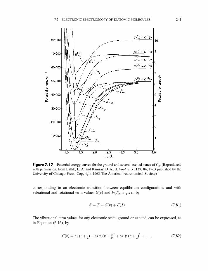
corresponding to an electronic transition between equilibrium configurations and with
vibrational and rotational term values GðvÞ and FðJ Þ, is given by
S ¼ T þ GðvÞ þ FðJ Þ ð7:81Þ
The vibrational term values for any electronic state, ground or excited, can be expressed, as
in Equation (6.16), by
GðvÞ ¼ oeðvþ 12Þ � oexeðvþ 1
2Þ2 þ oe yeðvþ 1
2Þ3 þ : : : ð7:82Þ
Figure 7.17 Potential energy curves for the ground and several excited states of C2. (Reproduced,
with permission, from Ballik, E. A. and Ramsay, D. A., Astrophys. J., 137, 84, 1963 published by the
University of Chicago Press; Copyright 1963 The American Astronomical Society)
7.2 ELECTRONIC SPECTROSCOPY OF DIATOMIC MOLECULES 241
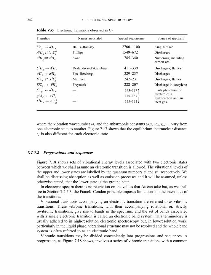
where the vibration wavenumber oe and the anharmonic constants oexe, oe ye, . . . vary fromone electronic state to another. Figure 7.17 shows that the equilibrium internuclear distance
re is also different for each electronic state.
7.2.5.2 Progressions and sequences
Figure 7.18 shows sets of vibrational energy levels associated with two electronic states
between which we shall assume an electronic transition is allowed. The vibrational levels of
the upper and lower states are labelled by the quantum numbers v0 and v00; respectively. We
shall be discussing absorption as well as emission processes and it will be assumed, unless
otherwise stated, that the lower state is the ground state.
In electronic spectra there is no restriction on the values that Dv can take but, as we shall
see in Section 7.2.5.3, the Franck–Condon principle imposes limitations on the intensities of
the transitions.
Vibrational transitions accompanying an electronic transition are referred to as vibronic
transitions. These vibronic transitions, with their accompanying rotational or, strictly,
rovibronic transitions, give rise to bands in the spectrum, and the set of bands associated
with a single electronic transition is called an electronic band system. This terminology is
usually adhered to in high-resolution electronic spectroscopy but, in low-resolution work,
particularly in the liquid phase, vibrational structure may not be resolved and the whole band
system is often referred to as an electronic band.
Vibronic transitions may be divided conveniently into progressions and sequences. A
progression, as Figure 7.18 shows, involves a series of vibronic transitions with a common
Table 7.6 Electronic transitions observed in C2
Transition Names associated Special region=nm Source of spectrum
b3S�g ! a3Pu Ballik–Ramsay 2700–1100 King furnace
A1Pg! X 1Sþg Phillips 1549–672 Discharges
d3Pg! a3Pu Swan 785–340 Numerous, including
carbon arc
C1Pg ! A1Pu Deslandres–d’Azambuja 411–339 Discharges, flames
e3Pg ! a3Pu Fox–Herzberg 329–237 Discharges
D1Sþu! X 1Sþg Mulliken 242–231 Discharges, flames
E1Sþg ! A1Pu Freymark 222–207 Discharge in acetylene
f 3S�g a3Pu — 143–137 Flash photolysis of
g3Dg a3Pu — 140–137mixture of a
F1Pu X 1Sþg — 135–131hydrocarbon and aninert gas
g
242 7 ELECTRONIC SPECTROSCOPY
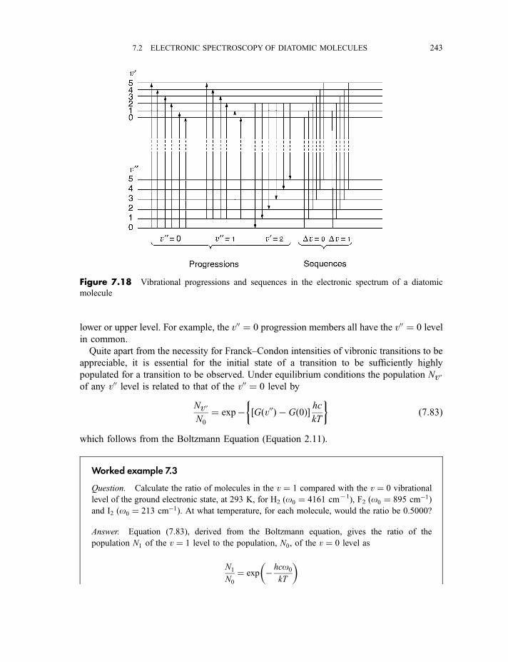
lower or upper level. For example, the v00 ¼ 0 progression members all have the v00 ¼ 0 level
in common.
Quite apart from the necessity for Franck–Condon intensities of vibronic transitions to be
appreciable, it is essential for the initial state of a transition to be sufficiently highly
populated for a transition to be observed. Under equilibrium conditions the population Nv00of any v00 level is related to that of the v00 ¼ 0 level by
Nv00N0
¼ exp� ½Gðv00Þ � Gð0Þ� hckT
�ð7:83Þ
which follows from the Boltzmann Equation (Equation 2.11).
Worked example 7.3
Question. Calculate the ratio of molecules in the v ¼ 1 compared with the v ¼ 0 vibrational
level of the ground electronic state, at 293 K, for H2 (o0 ¼ 4161 cm71), F2 ðo0 ¼ 895 cm�1Þand I2 ðo0 ¼ 213 cm�1Þ. At what temperature, for each molecule, would the ratio be 0.5000?
Answer. Equation (7.83), derived from the Boltzmann equation, gives the ratio of the
population N1 of the v ¼ 1 level to the population, N0, of the v ¼ 0 level as
N1
N0
¼ exp � hco0
kT
� �
Figure 7.18 Vibrational progressions and sequences in the electronic spectrum of a diatomic
molecule
7.2 ELECTRONIC SPECTROSCOPY OF DIATOMIC MOLECULES 243
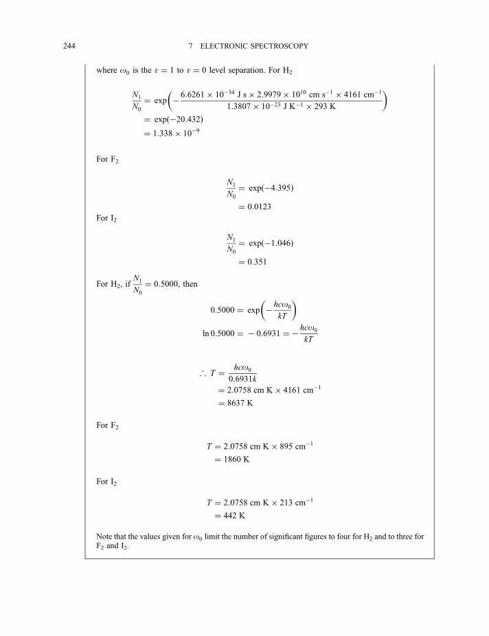
where o0 is the v ¼ 1 to v ¼ 0 level separation. For H2
N1
N0
¼ exp � 6:6261� 10�34 J s� 2:9979� 1010 cm s�1 � 4161 cm�1
1:3807� 10�23 J K�1 � 293 K
� �¼ expð�20:432Þ¼ 1:338� 10�9
For F2
N1
N0
¼ expð�4:395Þ
¼ 0:0123
For I2
N1
N0
¼ expð�1:046Þ
¼ 0:351
For H2, ifN1
N0
¼ 0:5000, then
0:5000 ¼ exp � hco0
kT
� �
ln 0:5000 ¼ � 0:6931 ¼ � hco0
kT
; T ¼ hco0
0:6931k
¼ 2:0758 cm K � 4161 cm�1
¼ 8637 K
For F2
T ¼ 2:0758 cm K � 895 cm�1
¼ 1860 K
For I2
T ¼ 2:0758 cm K � 213 cm�1
¼ 442 K
Note that the values given for o0 limit the number of significant figures to four for H2 and to three forF2 and I2.
244 7 ELECTRONIC SPECTROSCOPY
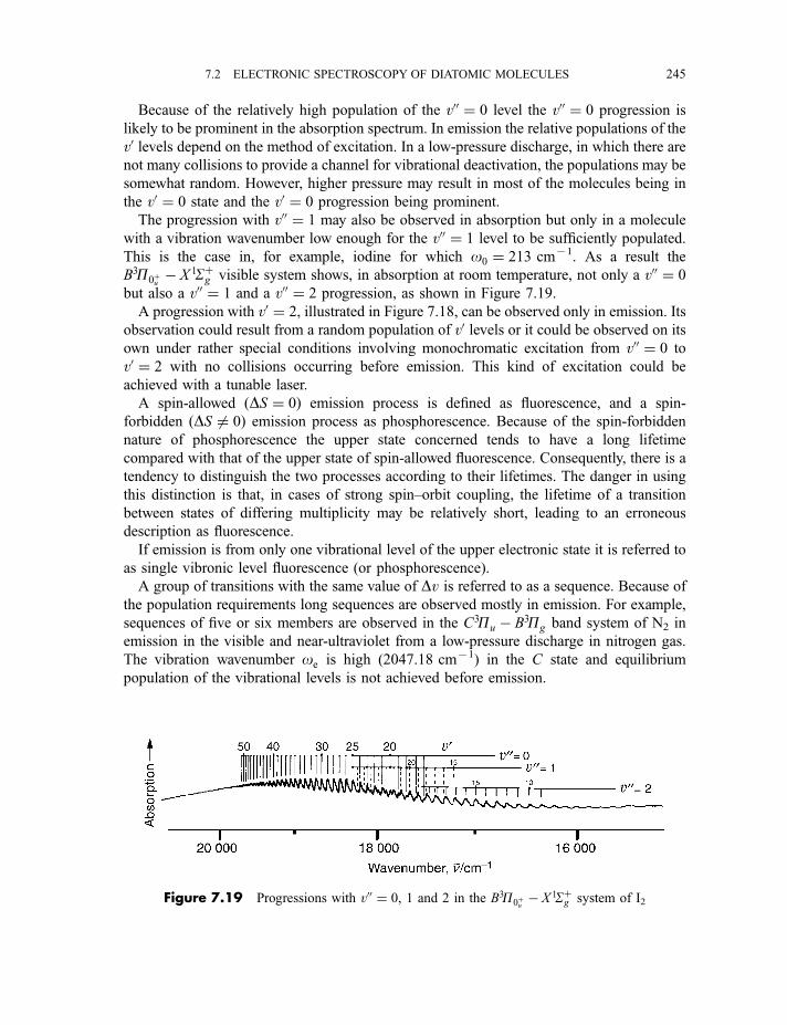
Because of the relatively high population of the v00 ¼ 0 level the v00 ¼ 0 progression is
likely to be prominent in the absorption spectrum. In emission the relative populations of the
v0 levels depend on the method of excitation. In a low-pressure discharge, in which there are
not many collisions to provide a channel for vibrational deactivation, the populations may be
somewhat random. However, higher pressure may result in most of the molecules being in
the v0 ¼ 0 state and the v0 ¼ 0 progression being prominent.
The progression with v00 ¼ 1 may also be observed in absorption but only in a molecule
with a vibration wavenumber low enough for the v00 ¼ 1 level to be sufficiently populated.
This is the case in, for example, iodine for which o0 ¼ 213 cm71. As a result the
B3P0þu � X 1Sþg visible system shows, in absorption at room temperature, not only a v00 ¼ 0
but also a v00 ¼ 1 and a v00 ¼ 2 progression, as shown in Figure 7.19.
A progression with v0 ¼ 2, illustrated in Figure 7.18, can be observed only in emission. Its
observation could result from a random population of v0 levels or it could be observed on its
own under rather special conditions involving monochromatic excitation from v00 ¼ 0 to
v0 ¼ 2 with no collisions occurring before emission. This kind of excitation could be
achieved with a tunable laser.
A spin-allowed ðDS ¼ 0Þ emission process is defined as fluorescence, and a spin-
forbidden ðDS 6¼ 0Þ emission process as phosphorescence. Because of the spin-forbidden
nature of phosphorescence the upper state concerned tends to have a long lifetime
compared with that of the upper state of spin-allowed fluorescence. Consequently, there is a
tendency to distinguish the two processes according to their lifetimes. The danger in using
this distinction is that, in cases of strong spin–orbit coupling, the lifetime of a transition
between states of differing multiplicity may be relatively short, leading to an erroneous
description as fluorescence.
If emission is from only one vibrational level of the upper electronic state it is referred to
as single vibronic level fluorescence (or phosphorescence).
A group of transitions with the same value of Dv is referred to as a sequence. Because of
the population requirements long sequences are observed mostly in emission. For example,
sequences of five or six members are observed in the C3Pu � B3Pg band system of N2 in
emission in the visible and near-ultraviolet from a low-pressure discharge in nitrogen gas.
The vibration wavenumber oe is high (2047.18 cm71) in the C state and equilibrium
population of the vibrational levels is not achieved before emission.
Figure 7.19 Progressions with v00 ¼ 0, 1 and 2 in the B3P0þu � X 1Sþg system of I2
7.2 ELECTRONIC SPECTROSCOPY OF DIATOMIC MOLECULES 245
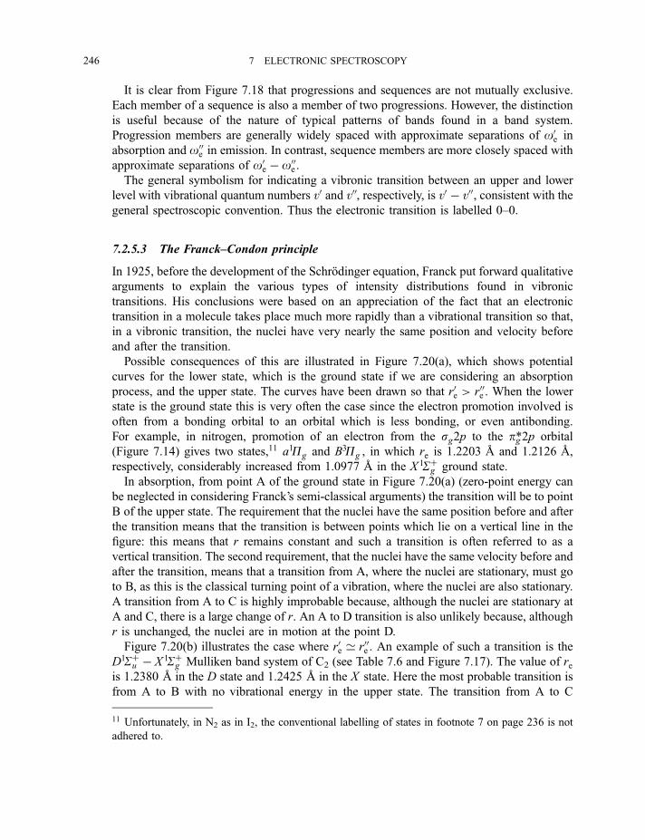
It is clear from Figure 7.18 that progressions and sequences are not mutually exclusive.
Each member of a sequence is also a member of two progressions. However, the distinction
is useful because of the nature of typical patterns of bands found in a band system.
Progression members are generally widely spaced with approximate separations of o0e in
absorption and o00e in emission. In contrast, sequence members are more closely spaced with
approximate separations of o0e � o00e .The general symbolism for indicating a vibronic transition between an upper and lower
level with vibrational quantum numbers v0 and v00, respectively, is v0 � v00, consistent with thegeneral spectroscopic convention. Thus the electronic transition is labelled 0–0.
7.2.5.3 The Franck–Condon principle
In 1925, before the development of the Schrodinger equation, Franck put forward qualitative
arguments to explain the various types of intensity distributions found in vibronic
transitions. His conclusions were based on an appreciation of the fact that an electronic
transition in a molecule takes place much more rapidly than a vibrational transition so that,
in a vibronic transition, the nuclei have very nearly the same position and velocity before
and after the transition.
Possible consequences of this are illustrated in Figure 7.20(a), which shows potential
curves for the lower state, which is the ground state if we are considering an absorption
process, and the upper state. The curves have been drawn so that r0e > r00e . When the lower
state is the ground state this is very often the case since the electron promotion involved is
often from a bonding orbital to an orbital which is less bonding, or even antibonding.
For example, in nitrogen, promotion of an electron from the sg2p to the pg*2p orbital
(Figure 7.14) gives two states,11 a1Pg and B3Pg , in which re is 1.2203 A and 1.2126 A,
respectively, considerably increased from 1.0977 A in the X 1Sþg ground state.
In absorption, from point A of the ground state in Figure 7.20(a) (zero-point energy can
be neglected in considering Franck’s semi-classical arguments) the transition will be to point
B of the upper state. The requirement that the nuclei have the same position before and after
the transition means that the transition is between points which lie on a vertical line in the
figure: this means that r remains constant and such a transition is often referred to as a
vertical transition. The second requirement, that the nuclei have the same velocity before and
after the transition, means that a transition from A, where the nuclei are stationary, must go
to B, as this is the classical turning point of a vibration, where the nuclei are also stationary.
A transition from A to C is highly improbable because, although the nuclei are stationary at
A and C, there is a large change of r. An A to D transition is also unlikely because, although
r is unchanged, the nuclei are in motion at the point D.
Figure 7.20(b) illustrates the case where r0e ’ r00e . An example of such a transition is the
D1Sþu � X 1Sþg Mulliken band system of C2 (see Table 7.6 and Figure 7.17). The value of reis 1.2380 A in the D state and 1.2425 A in the X state. Here the most probable transition is
from A to B with no vibrational energy in the upper state. The transition from A to C
11 Unfortunately, in N2 as in I2, the conventional labelling of states in footnote 7 on page 236 is not
adhered to.
246 7 ELECTRONIC SPECTROSCOPY
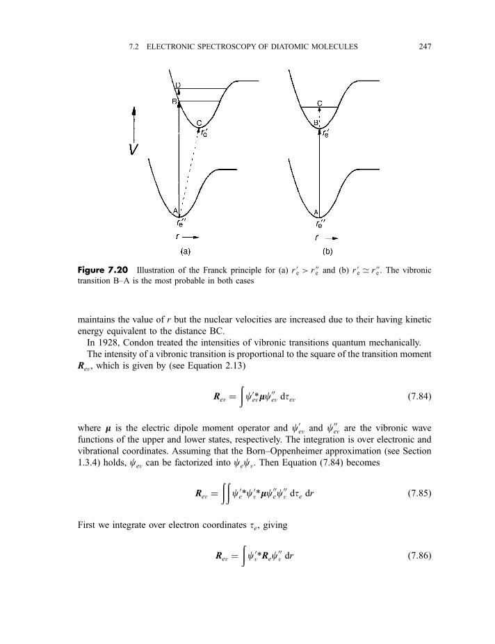
maintains the value of r but the nuclear velocities are increased due to their having kinetic
energy equivalent to the distance BC.
In 1928, Condon treated the intensities of vibronic transitions quantum mechanically.
The intensity of a vibronic transition is proportional to the square of the transition moment
Rev, which is given by (see Equation 2.13)
Rev ¼ðcev0*mmc00ev dtev ð7:84Þ
where mm is the electric dipole moment operator and c0ev and c00ev are the vibronic wave
functions of the upper and lower states, respectively. The integration is over electronic and
vibrational coordinates. Assuming that the Born–Oppenheimer approximation (see Section
1.3.4) holds, cev can be factorized into cecv. Then Equation (7.84) becomes
Rev ¼ðð
ce0*cv0*mmc00ec
00v dte dr ð7:85Þ
First we integrate over electron coordinates te, giving
Rev ¼ðcv0*Rec
00v dr ð7:86Þ
Figure 7.20 Illustration of the Franck principle for (a) r 0e > r 00e and (b) r 0e ’ r 00e . The vibronic
transition B–A is the most probable in both cases
7.2 ELECTRONIC SPECTROSCOPY OF DIATOMIC MOLECULES 247
where r is the internuclear distance and Re is the electronic transition moment given by
Re ¼ðce0*mmc00e dte ð7:87Þ
Our ability to do the integration to give Equation (7.86) is a consequence of the Born–
Oppenheimer approximation which assumes that the nuclei can be regarded as stationary in
relation to the much more fast-moving electrons. This approximation also allows us to take
Re outside the integral in Equation (7.86), regarding it as a constant, independent of r, which
is good enough for our purposes here. Thus we have
Rev ¼ Re
ðcv0*c00v dr ð7:88Þ
The quantityÐcv0*c00v dr is called the vibrational overlap integral, as it is a measure of the
degree to which the two vibrational wave functions overlap. Its square is known as the
Franck–Condon factor to which the intensity of the vibronic transition is proportional. In
carrying out the integration the requirement that r remain constant during the transition is
necessarily taken into account.
The classical turning point of a vibration, where nuclear velocities are zero, is replaced in
quantum mechanics by a maximum, or minimum, in cv near to this turning point. As is
illustrated in Figure 1.13 the larger is v the closer is the maximum, or minimum, in cv to the
classical turning point.
Figure 7.21 illustrates a particular case where the maximum of the v0 ¼ 4 wave function
near to the classical turning point is vertically above that of the v00 ¼ 0 wave function. The
maximum contribution to the vibrational overlap integral is indicated by the solid line, but
appreciable contributions extend to values of r within the dashed lines. Clearly, overlap
integrals for v0 close to four are also appreciable and give an intensity distribution in the
v00 ¼ 0 progression like that in Figure 7.22(b).
If r0e r00e there may be appreciable intensity involving the continuum of vibrational
levels above the dissociation limit. This results in a v00 ¼ 0 progression like that in Figure
7.22(c) where the intensity maximum is at a high value of v; or it may be in the continuum.
An example of this is the B3P0þu � X 1Sþg transition of iodine. In the B and X states re is
3.025 A and 2.666 A, respectively, leading to the broad intensity maximum close to the
continuum, as observed in Figure 7.19.
Figure 7.22(a) shows the intensity maximum at v0 ¼ 0 for the case when r0e ’ r00e . Theintensity usually falls off rapidly in such a case.
Occasionally, we encounter a case where r0e < r00e . When the lower state is the ground state
this is unusual but it can happen when the electron promotion is from an antibonding to a
non-bonding or bonding orbital. The situation is more likely to arise in a transition between
two excited states. Qualitatively, the situation is similar to that in Figure 7.21 except that the
upper potential curve is displaced to low r so that the right-hand maximum of, for example,
v0 ¼ 4 is above the v00 ¼ 0 maximum. The result is, again, an intensity distribution like that
in Figure 7.22(b) so that an observation of a long v00 ¼ 0 progression with an intensity
248 7 ELECTRONIC SPECTROSCOPY
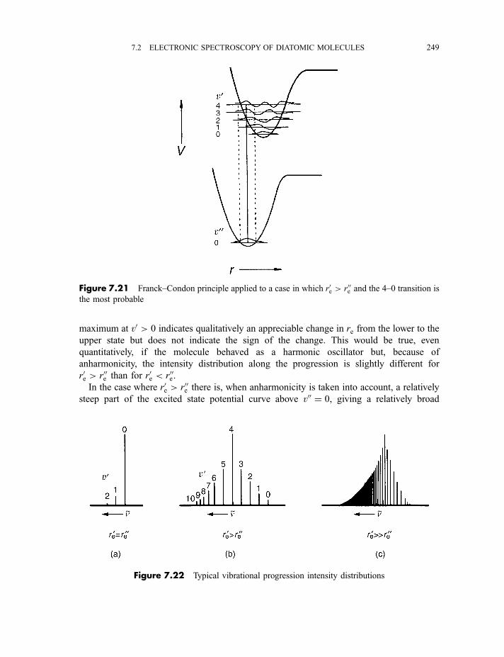
maximum at v0 > 0 indicates qualitatively an appreciable change in re from the lower to the
upper state but does not indicate the sign of the change. This would be true, even
quantitatively, if the molecule behaved as a harmonic oscillator but, because of
anharmonicity, the intensity distribution along the progression is slightly different for
r0e > r00e than for r0e < r00e.In the case where r0e > r00e there is, when anharmonicity is taken into account, a relatively
steep part of the excited state potential curve above v00 ¼ 0, giving a relatively broad
Figure 7.21 Franck–Condon principle applied to a case in which r0e > r00e and the 4–0 transition is
the most probable
Figure 7.22 Typical vibrational progression intensity distributions
7.2 ELECTRONIC SPECTROSCOPY OF DIATOMIC MOLECULES 249
maximum in the progression intensity. For r0e < r00e , there is a shallower part of the excited
state potential curve above v00 ¼ 0 and a sharper intensity maximum results.
Accurate intensity measurements have been made in many cases and calculations of
r0e � r00e made, including the effects of anharmonicity and even allowing for breakdown of the
Born–Oppenheimer approximation.
7.2.5.4 Deslandres tables
The illustration of various types of vibronic transitions in Figure 7.18 suggests that we can
use the method of combination differences to obtain the separations of vibrational levels
from observed transition wavenumbers. This method was introduced in Section 6.1.4.1 and
was applied to obtaining rotational constants for two combining vibrational states. The
method works on the simple principle that, if two transitions have an upper level in common,
their wavenumber difference is a function of lower state parameters only, and vice versa if
they have a lower level in common.
In using the combination difference method to obtain vibrational parameters, oe, oexe,
etc., for two electronic states between which vibronic transitions are observed, the first step
is to organize all the vibronic transition wavenumbers into a Deslandres table. An example is
shown in Table 7.7 for the A1P� X 1Sþ system of carbon monoxide. The electronic
transition results from an electron promotion which, because of the similarity of the two
nuclei, can be described approximately in terms of the MO diagram for homonuclear
diatomic molecules shown in Figure 7.14. Carbon monoxide is isoelectronic with the
nitrogen molecule so the lowest-energy electron promotion is from s2p to p*2p (the ‘g’ and
‘u’ subscripts do not apply to heteronuclear diatomic molecules). The promotion gives two
states, A1P and a3P. The A1P� X 1Sþ band system lies in the far-ultraviolet region of the
spectrum, with the 0–0 band at 154.5 nm.
In Table 7.7, all the transition wavenumbers have been arranged in rows and columns so
that the differences between wavenumbers in adjacent columns correspond to vibrational
level separations in the lower (ground) electronic state and the differences between adjacent
rows to separations in the upper electronic state. These differences are shown in parentheses.
The variations of the differences (e.g. between the first two columns), are a result of
uncertainties in the experimental measurements.
From the table a series of averaged values of vibrational term value differences,
Gðvþ 1Þ � GðvÞ, can be obtained for both electronic states and, from Equation (6.18),
values of oe, oexe, etc., for both states. For example, in the A1P and X 1Sþ states of CO, oe
is 1518.2 cm71 and 2169.8 cm71, respectively. The large decrease in oe in the A state is a
consequence of promoting an electron from a bonding to an antibonding orbital, greatly
reducing the force constant.
7.2.5.5 Dissociation energies
If a sufficient number of vibrational term values are known in any electronic state the
dissociation energy D0 can be obtained from a Birge–Sponer extrapolation, as discussed in
250 7 ELECTRONIC SPECTROSCOPY
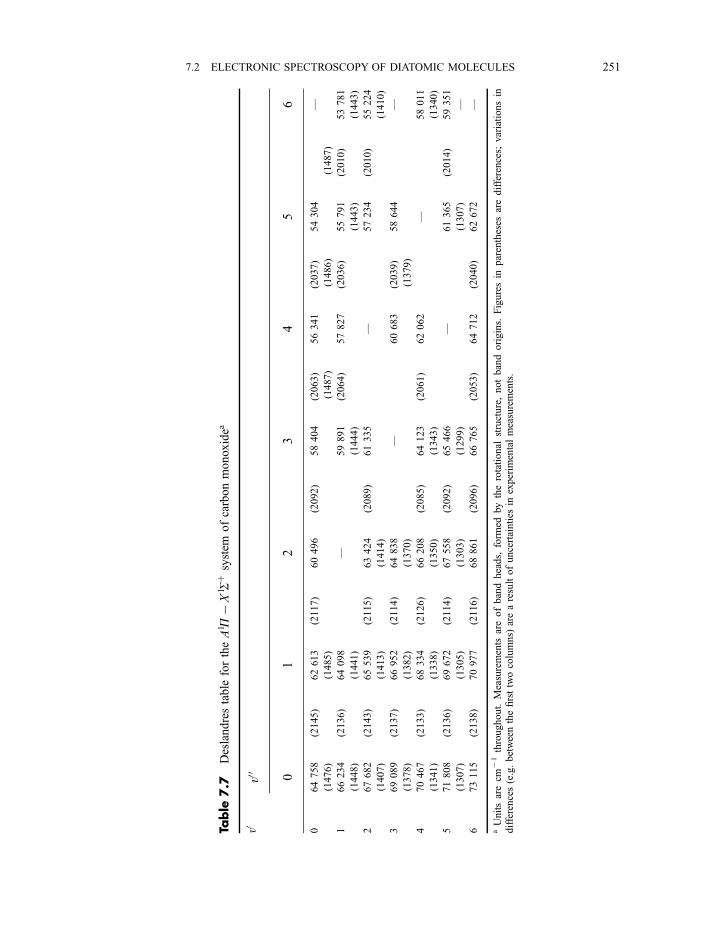
Table
7.7
Deslandrestable
fortheA1 P�X
1 Sþsystem
ofcarbonmonoxidea
v0v00
01
23
45
6
064758
(2145)
62613
(2117)
60496
(2092)
58404
(2063)
56341
(2037)
54304
—
(1476)
(1485)
(1487)
(1486)
(1487)
166234
(2136)
64098
—59891
(2064)
57827
(2036)
55791
(2010)
53781
(1448)
(1441)
(1444)
(1443)
(1443)
267682
(2143)
65539
(2115)
63424
(2089)
61335
—57234
(2010)
55224
(1407)
(1413)
(1414)
(1410)
369089
(2137)
66952
(2114)
64838
—60683
(2039)
58644
—
(1378)
(1382)
(1370)
(1379)
470467
(2133)
68334
(2126)
66208
(2085)
64123
(2061)
62062
—58011
(1341)
(1338)
(1350)
(1343)
(1340)
571808
(2136)
69672
(2114)
67558
(2092)
65466
—61365
(2014)
59351
(1307)
(1305)
(1303)
(1299)
(1307)
—
673115
(2138)
70977
(2116)
68861
(2096)
66765
(2053)
64712
(2040)
62672
—
aUnitsarecm
71throughout.Measurements
areofbandheads,
form
edbytherotational
structure,notbandorigins.
Figuresin
parentheses
aredifferences;
variationsin
differences(e.g.betweenthefirsttwocolumns)
arearesultofuncertainties
inexperim
entalmeasurements.
7.2 ELECTRONIC SPECTROSCOPY OF DIATOMIC MOLECULES 251
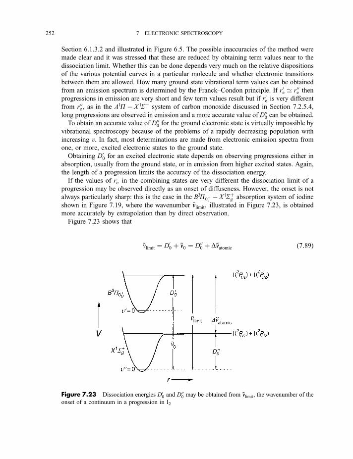
Section 6.1.3.2 and illustrated in Figure 6.5. The possible inaccuracies of the method were
made clear and it was stressed that these are reduced by obtaining term values near to the
dissociation limit. Whether this can be done depends very much on the relative dispositions
of the various potential curves in a particular molecule and whether electronic transitions
between them are allowed. How many ground state vibrational term values can be obtained
from an emission spectrum is determined by the Franck–Condon principle. If r0e ’ r00e then
progressions in emission are very short and few term values result but if r0e is very different
from r00e , as in the A1P� X 1Sþ system of carbon monoxide discussed in Section 7.2.5.4,
long progressions are observed in emission and a more accurate value of D000 can be obtained.To obtain an accurate value of D000 for the ground electronic state is virtually impossible by
vibrational spectroscopy because of the problems of a rapidly decreasing population with
increasing v. In fact, most determinations are made from electronic emission spectra from
one, or more, excited electronic states to the ground state.
Obtaining D00 for an excited electronic state depends on observing progressions either in
absorption, usually from the ground state, or in emission from higher excited states. Again,
the length of a progression limits the accuracy of the dissociation energy.
If the values of re in the combining states are very different the dissociation limit of a
progression may be observed directly as an onset of diffuseness. However, the onset is not
always particularly sharp: this is the case in the B3P0þu � X 1Sþg absorption system of iodine
shown in Figure 7.19, where the wavenumber ~nnlimit; illustrated in Figure 7.23, is obtained
more accurately by extrapolation than by direct observation.
Figure 7.23 shows that
~nnlimit ¼ D00 þ ~nn0 ¼ D000 þ D~nnatomic ð7:89Þ
Figure 7.23 Dissociation energies D00 and D000 may be obtained from ~nnlimit, the wavenumber of the
onset of a continuum in a progression in I2
252 7 ELECTRONIC SPECTROSCOPY
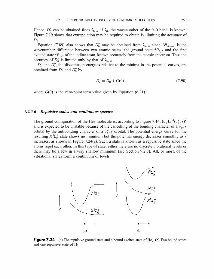
Hence, D00 can be obtained from ~nnlimit if ~nn0, the wavenumber of the 0–0 band, is known.
Figure 7.19 shows that extrapolation may be required to obtain ~nn0, limiting the accuracy of
D00.Equation (7.89) also shows that D000 may be obtained from ~nnlimit since D~nnatomic is the
wavenumber difference between two atomic states, the ground state 2P3=2 and the first
excited state 2P1=2 of the iodine atom, known accurately from the atomic spectrum. Thus the
accuracy of D000 is limited only by that of ~nnlimit.
D0e and D00e, the dissociation energies relative to the minima in the potential curves, are
obtained from D00 and D000 by
De ¼ D0 þ Gð0Þ ð7:90Þ
where Gð0Þ is the zero-point term value given by Equation (6.21).
7.2.5.6 Repulsive states and continuous spectra
The ground configuration of the He2 molecule is, according to Figure 7.14, ðsg1sÞ2ðsu*1sÞ2and is expected to be unstable because of the cancelling of the bonding character of a sg1sorbital by the antibonding character of a su*1s orbital. The potential energy curve for the
resulting X 1Sþg state shows no minimum but the potential energy decreases smoothly as r
increases, as shown in Figure 7.24(a). Such a state is known as a repulsive state since the
atoms repel each other. In this type of state, either there are no discrete vibrational levels or
there may be a few in a very shallow minimum (see Section 9.2.8). All, or most, of the
vibrational states form a continuum of levels.
Figure 7.24 (a) The repulsive ground state and a bound excited state of He2. (b) Two bound states
and one repulsive state of H2
7.2 ELECTRONIC SPECTROSCOPY OF DIATOMIC MOLECULES 253
Promotion of an electron in He2 from the su*1s to a bonding orbital produces some bound
states of the molecule of which several have been characterized in emission spectroscopy.
For example, the configuration ðsg1sÞ2ðsu*1sÞ1ðsg2sÞ1 gives rise to the A1Sþu and a3Sþu bound
states. Figure 7.24(a) shows the form of the potential curve for the A1Sþu state. The A–X
transition is allowed and gives rise to an intense continuum in emission between 60 nm and
100 nm. This is used as a far-ultraviolet continuum source (see Section 3.4.5) as are the
corresponding continua from other noble gas diatomic molecules.
Another example of a continuous emission spectrum is that from a discharge in molecular
hydrogen. It covers the range from 160 nm to 500 nm and is used as a visible and near-
ultraviolet continuum source (see Section 3.4.4). The transition involved is from the bound
a3Sþg to the repulsive b3Sþu state, shown in Figure 7.24(b) and arising from the excited
configuration ðsg1sÞ1ðsu*1sÞ1. The dissociation products are two ground state ð12S1=2Þhydrogen atoms, the same as for the X 1Sþg ground state. The a3Sþg state arises from the
configuration ðsg1sÞ1ðsg2sÞ1.
7.2.6 Rotational fine structure
For electronic or vibronic transitions there is a set of accompanying rotational transitions
between the stacks of rotational levels associated with the upper and lower electronic or
vibronic states, in a rather similar way to infrared vibrational transitions (Section 6.1.4.1).
The main differences are caused by there being a wider range of electronic or vibronic
transitions: they are not confined to S� S types and the upper and lower states may not be
singlet states nor need their multiplicities to be the same. These possibilities result in a
variety of types of rotational fine structure, but we shall confine ourselves to 1S� 1S and1P� 1S types of transitions only.
7.2.6.1 1S 2 1S electronic and vibronic transitions
In Figure 7.25 are shown stacks of rotational levels associated with two 1Sþ electronic states
between which a transition is allowed by the þ $ þ and, if it is a homonuclear diatomic,
g$ u selection rules of Equations (7.70) and (7.71). The sets of levels would be similar if
both were S� states or if the upper state were ‘g’ and the lower state ‘u’. The rotational term
values for any 1S state are given by the expression encountered first in Equation (5.23),
namely
FvðJ Þ ¼ BvJ ðJ þ 1Þ � DvJ2ðJ þ 1Þ2 ð7:91Þ
where Bv is the rotational constant (Equations 5.11 and 5.12), Dv is a centrifugal distortion
constant, and the subscripts ‘v’ indicate the vibrational dependence of these. Only the v-dependence of Bv is important here and it is given by
Bv ¼ Be � aðvþ 12Þ ð7:92Þ
254 7 ELECTRONIC SPECTROSCOPY
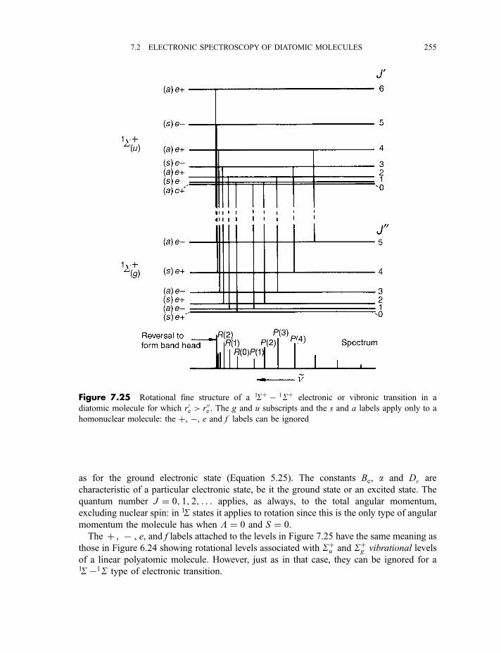
as for the ground electronic state (Equation 5.25). The constants Be, a and Dv are
characteristic of a particular electronic state, be it the ground state or an excited state. The
quantum number J ¼ 0; 1; 2; . . . applies, as always, to the total angular momentum,
excluding nuclear spin: in 1S states it applies to rotation since this is the only type of angular
momentum the molecule has when L ¼ 0 and S ¼ 0.
The þ , 7 , e, and f labels attached to the levels in Figure 7.25 have the same meaning as
those in Figure 6.24 showing rotational levels associated with Sþu and Sþg vibrational levels
of a linear polyatomic molecule. However, just as in that case, they can be ignored for a1S�1S type of electronic transition.
Figure 7.25 Rotational fine structure of a 1Sþ � 1Sþ electronic or vibronic transition in a
diatomic molecule for which r0e > r00e . The g and u subscripts and the s and a labels apply only to a
homonuclear molecule: the þ, �, e and f labels can be ignored
7.2 ELECTRONIC SPECTROSCOPY OF DIATOMIC MOLECULES 255
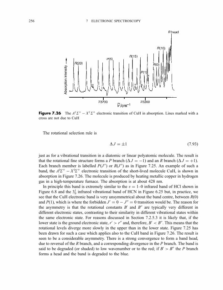
The rotational selection rule is
D J ¼ �1 ð7:93Þ
just as for a vibrational transition in a diatomic or linear polyatomic molecule. The result is
that the rotational fine structure forms a P branch ðD J ¼ �1Þ and an R branch ðD J ¼ þ1Þ.Each branch member is labelled PðJ 00Þ or RðJ 00Þ as in Figure 7.25. An example of such a
band, the A1Sþ � X 1Sþ electronic transition of the short-lived molecule CuH, is shown in
absorption in Figure 7.26. The molecule is produced by heating metallic copper in hydrogen
gas in a high-temperature furnace. The absorption is at about 428 nm.
In principle this band is extremely similar to the v ¼ 1–0 infrared band of HCl shown in
Figure 6.8 and the 310 infrared vibrational band of HCN in Figure 6.25 but, in practice, we
see that the CuH electronic band is very unsymmetrical about the band centre, between Rð0Þand Pð1Þ, which is where the forbidden J 0 ¼ 0 � J 00 ¼ 0 transition would be. The reason for
the asymmetry is that the rotational constants B0 and B00 are typically very different in
different electronic states, contrasting to their similarity in different vibrational states within
the same electronic state. For reasons discussed in Section 7.2.5.3 it is likely that, if the
lower state is the ground electronic state, r0 > r00 and, therefore, B0 < B00. This means that the
rotational levels diverge more slowly in the upper than in the lower state. Figure 7.25 has
been drawn for such a case which applies also to the CuH band in Figure 7.26. The result is
seen to be a considerable asymmetry. There is a strong convergence to form a band head,
due to reversal of the R branch, and a corresponding divergence in the P branch. The band is
said to be degraded (or shaded) to low wavenumber or to the red; if B0 > B00 the P branch
forms a head and the band is degraded to the blue.
Figure 7.26 The A1Sþ � X 1Sþ electronic transition of CuH in absorption. Lines marked with a
cross are not due to CuH
256 7 ELECTRONIC SPECTROSCOPY
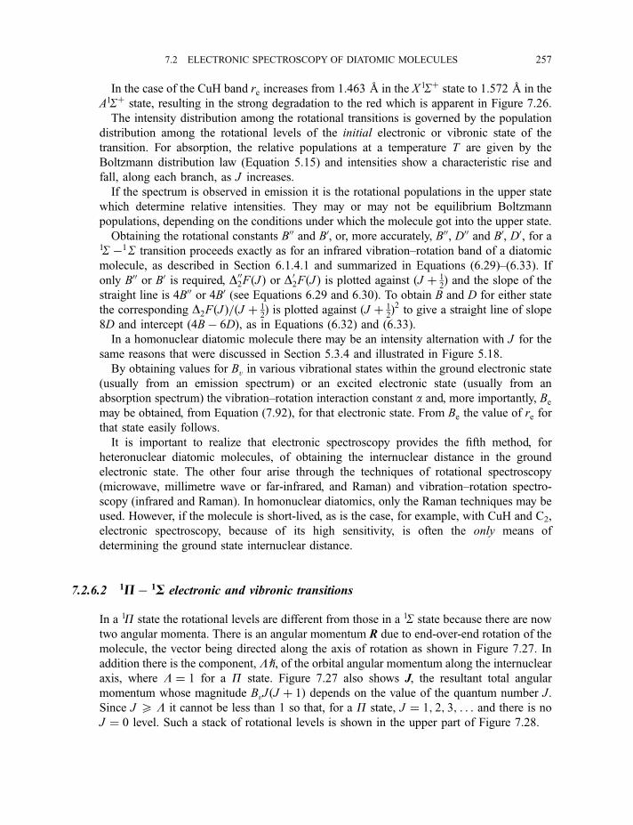
In the case of the CuH band re increases from 1.463 A in the X 1Sþ state to 1.572 A in the
A1Sþ state, resulting in the strong degradation to the red which is apparent in Figure 7.26.
The intensity distribution among the rotational transitions is governed by the population
distribution among the rotational levels of the initial electronic or vibronic state of the
transition. For absorption, the relative populations at a temperature T are given by the
Boltzmann distribution law (Equation 5.15) and intensities show a characteristic rise and
fall, along each branch, as J increases.
If the spectrum is observed in emission it is the rotational populations in the upper state
which determine relative intensities. They may or may not be equilibrium Boltzmann
populations, depending on the conditions under which the molecule got into the upper state.
Obtaining the rotational constants B00 and B0, or, more accurately, B00, D00 and B0, D0, for a1S�1S transition proceeds exactly as for an infrared vibration–rotation band of a diatomic
molecule, as described in Section 6.1.4.1 and summarized in Equations (6.29)–(6.33). If
only B00 or B0 is required, D002FðJ Þ or D02FðJ Þ is plotted against ðJ þ 12Þ and the slope of the
straight line is 4B00 or 4B0 (see Equations 6.29 and 6.30). To obtain B and D for either state
the corresponding D2FðJ Þ=ðJ þ 12Þ is plotted against ðJ þ 1
2Þ2 to give a straight line of slope
8D and intercept ð4B� 6DÞ, as in Equations (6.32) and (6.33).
In a homonuclear diatomic molecule there may be an intensity alternation with J for the
same reasons that were discussed in Section 5.3.4 and illustrated in Figure 5.18.
By obtaining values for Bv in various vibrational states within the ground electronic state
(usually from an emission spectrum) or an excited electronic state (usually from an
absorption spectrum) the vibration–rotation interaction constant a and, more importantly, Be
may be obtained, from Equation (7.92), for that electronic state. From Be the value of re for
that state easily follows.
It is important to realize that electronic spectroscopy provides the fifth method, for
heteronuclear diatomic molecules, of obtaining the internuclear distance in the ground
electronic state. The other four arise through the techniques of rotational spectroscopy
(microwave, millimetre wave or far-infrared, and Raman) and vibration–rotation spectro-
scopy (infrared and Raman). In homonuclear diatomics, only the Raman techniques may be
used. However, if the molecule is short-lived, as is the case, for example, with CuH and C2,
electronic spectroscopy, because of its high sensitivity, is often the only means of
determining the ground state internuclear distance.
7.2.6.2 1P � 1S electronic and vibronic transitions
In a 1P state the rotational levels are different from those in a 1S state because there are now
two angular momenta. There is an angular momentum R due to end-over-end rotation of the
molecule, the vector being directed along the axis of rotation as shown in Figure 7.27. In
addition there is the component, Lh, of the orbital angular momentum along the internuclear
axis, where L ¼ 1 for a P state. Figure 7.27 also shows J, the resultant total angular
momentum whose magnitude BvJ ðJ þ 1Þ depends on the value of the quantum number J.
Since J 5 L it cannot be less than 1 so that, for a P state, J ¼ 1; 2; 3; . . . and there is no
J ¼ 0 level. Such a stack of rotational levels is shown in the upper part of Figure 7.28.
7.2 ELECTRONIC SPECTROSCOPY OF DIATOMIC MOLECULES 257
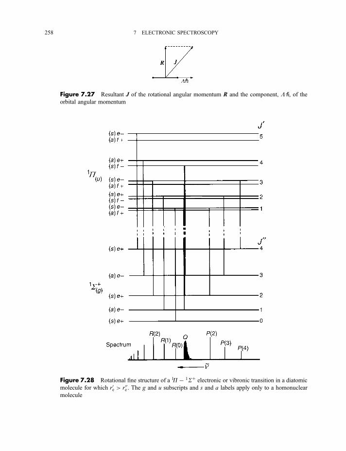
Figure 7.27 Resultant J of the rotational angular momentum R and the component, L h, of the
orbital angular momentum
Figure 7.28 Rotational fine structure of a 1P� 1Sþ electronic or vibronic transition in a diatomic
molecule for which r0e > r00e . The g and u subscripts and s and a labels apply only to a homonuclear
molecule
258 7 ELECTRONIC SPECTROSCOPY
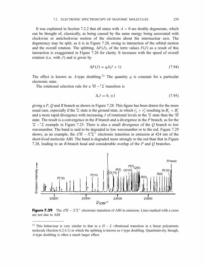
It was explained in Section 7.2.2 that all states with L > 0 are doubly degenerate, which
can be thought of, classically, as being caused by the same energy being associated with
clockwise or anticlockwise motion of the electrons about the internuclear axis. The
degeneracy may be split, as it is in Figure 7.28, owing to interaction of the orbital motion
and the overall rotation. The splitting, DFðJ Þ, of the term values FðJ Þ as a result of this
interaction is exaggerated in Figure 7.28 for clarity. It increases with the speed of overall
rotation (i.e. with J ) and is given by
DFðJ Þ ¼ qJ ðJ þ 1Þ ð7:94Þ
The effect is known as L-type doubling.12 The quantity q is constant for a particular
electronic state.
The rotational selection rule for a 1P�1S transition is
D J ¼ 0;�1 ð7:95Þ
giving a P, Q and R branch as shown in Figure 7.28. This figure has been drawn for the more
usual case, especially if the 1S state is the ground state, in which r0e > r00e resulting in B0e < B00eand a more rapid divergence with increasing J of rotational levels in the 1S state than the 1Pstate. The result is a convergence in the R branch and a divergence in the P branch, as for the1S�1S example in Figure 7.25. There is also a small divergence of the Q branch to low
wavenumber. The band is said to be degraded to low wavenumber or to the red. Figure 7.29
shows, as an example, the A1P� X 1Sþ electronic transition in emission at 424 nm of the
short-lived molecule AlH. The band is degraded more strongly to the red than that in Figure
7.28, leading to an R-branch head and considerable overlap of the P and Q branches.
12 This behaviour is very similar to that in a P� S vibrational transition in a linear polyatomic
molecule (Section 6.2.4.1) in which the splitting is known as ‘-type doubling. Quantitatively, though,L-type doubling is often a much larger effect.
Figure 7.29 The A1P� X 1Sþ electronic transition of AlH in emission. Lines marked with a cross
are not due to AlH
7.2 ELECTRONIC SPECTROSCOPY OF DIATOMIC MOLECULES 259
Whereas the þ and 7 or e and f labels attached to the rotational levels for a 1S� 1Stransition in Figure 7.25 were superfluous, so far as rotational selection rules were
concerned, they are essential for a 1P� 1S transition in order to tell us which of the split
components in the 1P state is involved in a particular transition.
The þ or 7 label indicates whether the wave function is symmetric or antisymmetric,
respectively, to reflection across any plane containing the internuclear axis. Whether the þcomponent is below or above the 7 component for, say, J ¼ 1 depends on the sign of q in
Equation (7.94). The selection rules13
þ $ �;þ $j þ;� $j � ð7:96Þ
result in the P and R branches involving the upper components and the Q branch the lower
components for the case in Figure 7.28. The selection rules
e$ f ; e$j e; f $j f for D J ¼ 0; e$j f ; e$ e; f $ f for D J ¼ �1 ð7:97Þ
involving the alternative e or f labels lead to exactly the same result.
The method of combination differences applied to the P and R branches gives the lower
state rotational constants B00, or B00 and D00, just as in a 1S� 1S transition, from Equation
(6.29) or Equation (6.32). These branches also give rotational constants B0u, or B0u and D0u,relating to the upper components of the 1P state, from Equation (6.30) or Equation (6.33).
The constants B0‘, or B0‘ and D0‘, relating to the lower components of the 1P state, may be
obtained from the Q branch. The value of q can be obtained from B0u and B0‘.In the A1P� X 1Sþ electronic transition of AlH, shown in Figure 7.29, the considerable
degradation of the band to the red is due not to an appreciable geometry change, since re is
1.6478 A in the X 1Sþ state and 1.648 A in the A1P state, but to the relatively high value of q
of 0.0080 cm71 in the A1P state.
The ‘g’ and ‘u’ subscripts in Figure 7.28 are appropriate only to a homonuclear diatomic
molecule. This is the case also for the ‘s’ and ‘a’ labels which may result in intensity
alternations for J even or odd in the initial state of the transition. Figure 7.28 would apply
equally to a 1P� 1S� type of transition.
7.3 Electronic spectroscopy of polyatomic molecules
7.3.1 Molecular orbitals and electronic states
Polyatomic molecules cover such a wide range of different types that it is not possible here
to discuss the MOs and electron configurations of more than a very few. The molecules that
we shall discuss are those of the general type AH2, where A is a first-row element,
formaldehyde (H2CO), benzene and some regular octahedral transition metal complexes.
13 Note that these are the opposite of the electronic selection rules in Equation (7.70).
260 7 ELECTRONIC SPECTROSCOPY
For non-linear polyatomic molecules the use of symmetry arguments in discussing
orbitals and electronic states becomes almost essential, whereas for atoms and diatomic
molecules this could be largely avoided. For linear polyatomic molecules the classification
of orbitals and states and the description of electronic and associated rotational selection
rules are very similar to those for diatomic molecules: symmetry arguments, again, may be
largely avoided. However, it is possible that a polyatomic molecule which is linear in its
ground state may be non-linear in some excited electronic states. For example, acetylene
(HCCH) has a linear ground state ð1Sþg Þ but a trans bent first excited singlet state
necessitating the use of symmetry in discussing states, transitions, etc.
The total electron density contributed by all the electrons in any molecule is a property
that can be visualized and it is possible to imagine an experiment in which it could be
observed. It is when we try to break down this electron density into a contribution from each
electron that problems arise. The methods employing hybrid orbitals or equivalent orbitals
are useful in certain circumstances such as in rationalizing properties of a localized part of
the molecule. However, the promotion of an electron from one orbital to another, in an
electronic transition, or the complete removal of it, in an ionization process, both obey
symmetry selection rules. For this reason the orbitals used to describe the difference between
either two electronic states of the molecule or an electronic state of the molecule and an
electronic state of the positive ion must be MOs which belong to symmetry species of the
point group to which the molecule belongs. Such orbitals are called symmetry orbitals and
are the only type we shall consider here.
7.3.1.1 AH2 molecules
The valence atomic orbitals (AOs) of A and H are the most important, so far as the valence
MOs of AH2 are concerned, and these are 2s and 2p of the first-row element A (Li to Ne)
and the 1s AO on H.
AH2 molecules may have two possible extreme geometries: linear, belonging to the D1h
point group, or bent with an angle of 90�, belonging to the C2v point group. We shall
construct MOs for these two extremes and see how they correlate as the angle changes
smoothly from 90� to 180�.
7.3.1.1(a) ffHAH¼ 180� The 2s and 2p orbitals on A and the 1s orbital on H must be
assigned to symmetry species of the D1h point group (see Table A.37 in Appendix A for the
character table). The spherically symmetrical 2s orbital belongs to the species sþg , the 2pzAO, where z is the internuclear axis, belongs to sþu , and the 2px and 2py AOs, which remain
degenerate, belong to pu. A 1s orbital on H cannot, by itself, be assigned to a symmetry
species. We get over this problem by taking in-phase and out-of-phase combinations of both
of them, as shown in Figure 7.30. The resulting orbitals belong to the sþg and sþu symmetry
species, respectively. The way in which the MOs are formed is indicated on the right-hand
side of Figure 7.31.
The requirements for formation of MOs are the same as for a diatomic molecule, namely,
that the orbitals from which they are formed must be of comparable energy and of the right
7.3 ELECTRONIC SPECTROSCOPY OF POLYATOMIC MOLECULES 261
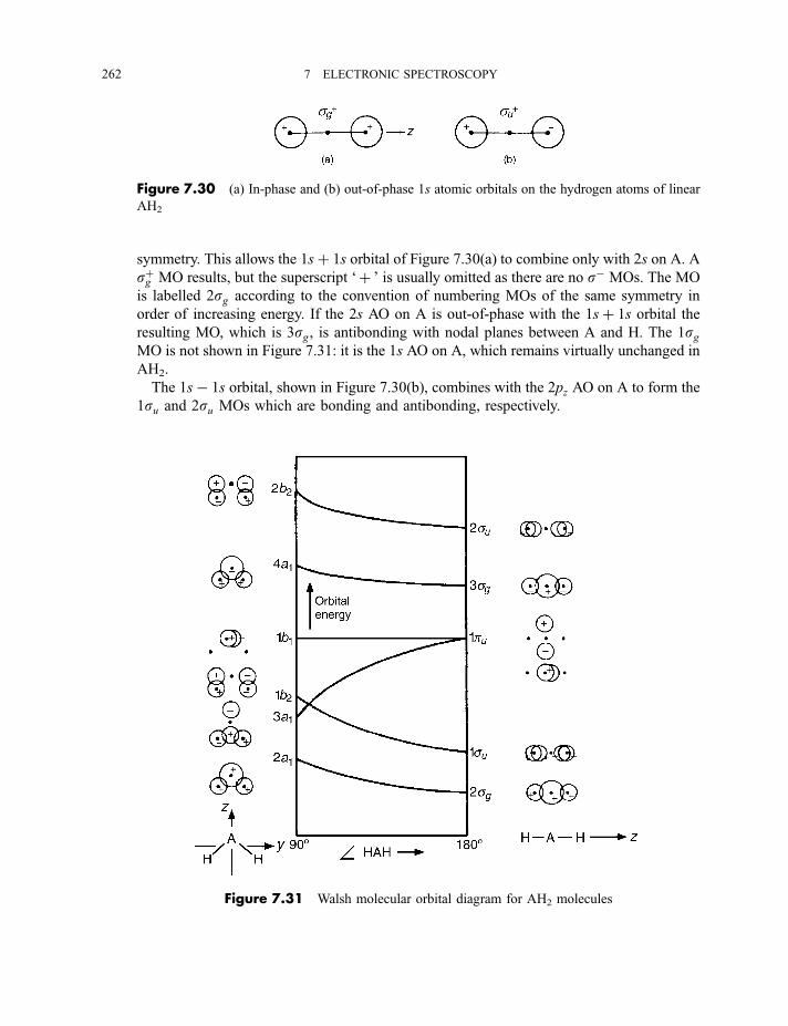
symmetry. This allows the 1sþ 1s orbital of Figure 7.30(a) to combine only with 2s on A. A
sþg MO results, but the superscript ‘þ ’ is usually omitted as there are no s� MOs. The MO
is labelled 2sg according to the convention of numbering MOs of the same symmetry in
order of increasing energy. If the 2s AO on A is out-of-phase with the 1sþ 1s orbital the
resulting MO, which is 3sg, is antibonding with nodal planes between A and H. The 1sgMO is not shown in Figure 7.31: it is the 1s AO on A, which remains virtually unchanged in
AH2.
The 1s� 1s orbital, shown in Figure 7.30(b), combines with the 2pz AO on A to form the
1su and 2su MOs which are bonding and antibonding, respectively.
Figure 7.31 Walsh molecular orbital diagram for AH2 molecules
Figure 7.30 (a) In-phase and (b) out-of-phase 1s atomic orbitals on the hydrogen atoms of linear
AH2
262 7 ELECTRONIC SPECTROSCOPY
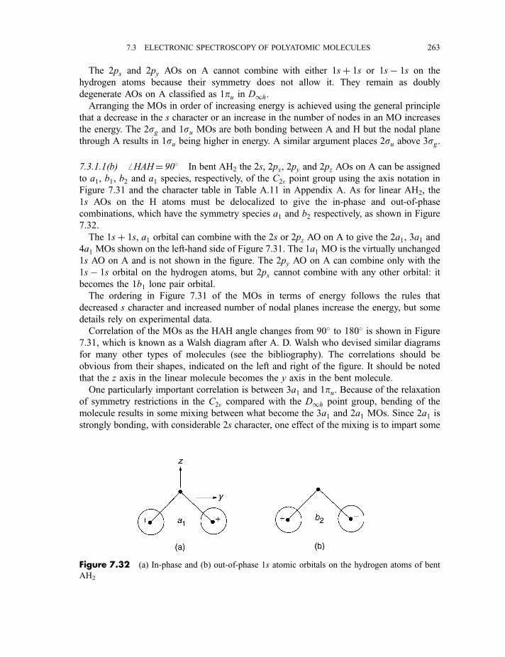
The 2px and 2py AOs on A cannot combine with either 1sþ 1s or 1s� 1s on the
hydrogen atoms because their symmetry does not allow it. They remain as doubly
degenerate AOs on A classified as 1pu in D1h.
Arranging the MOs in order of increasing energy is achieved using the general principle
that a decrease in the s character or an increase in the number of nodes in an MO increases
the energy. The 2sg and 1su MOs are both bonding between A and H but the nodal plane
through A results in 1su being higher in energy. A similar argument places 2su above 3sg.
7.3.1.1(b) ffHAH¼ 90� In bent AH2 the 2s, 2px, 2py and 2pz AOs on A can be assigned
to a1, b1, b2 and a1 species, respectively, of the C2v point group using the axis notation in
Figure 7.31 and the character table in Table A.11 in Appendix A. As for linear AH2, the
1s AOs on the H atoms must be delocalized to give the in-phase and out-of-phase
combinations, which have the symmetry species a1 and b2 respectively, as shown in Figure
7.32.
The 1sþ 1s, a1 orbital can combine with the 2s or 2pz AO on A to give the 2a1, 3a1 and
4a1 MOs shown on the left-hand side of Figure 7.31. The 1a1 MO is the virtually unchanged
1s AO on A and is not shown in the figure. The 2py AO on A can combine only with the
1s� 1s orbital on the hydrogen atoms, but 2px cannot combine with any other orbital: it
becomes the 1b1 lone pair orbital.
The ordering in Figure 7.31 of the MOs in terms of energy follows the rules that
decreased s character and increased number of nodal planes increase the energy, but some
details rely on experimental data.
Correlation of the MOs as the HAH angle changes from 90� to 180� is shown in Figure
7.31, which is known as a Walsh diagram after A. D. Walsh who devised similar diagrams
for many other types of molecules (see the bibliography). The correlations should be
obvious from their shapes, indicated on the left and right of the figure. It should be noted
that the z axis in the linear molecule becomes the y axis in the bent molecule.
One particularly important correlation is between 3a1 and 1pu. Because of the relaxationof symmetry restrictions in the C2v compared with the D1h point group, bending of the
molecule results in some mixing between what become the 3a1 and 2a1 MOs. Since 2a1 is
strongly bonding, with considerable 2s character, one effect of the mixing is to impart some
Figure 7.32 (a) In-phase and (b) out-of-phase 1s atomic orbitals on the hydrogen atoms of bent
AH2
7.3 ELECTRONIC SPECTROSCOPY OF POLYATOMIC MOLECULES 263
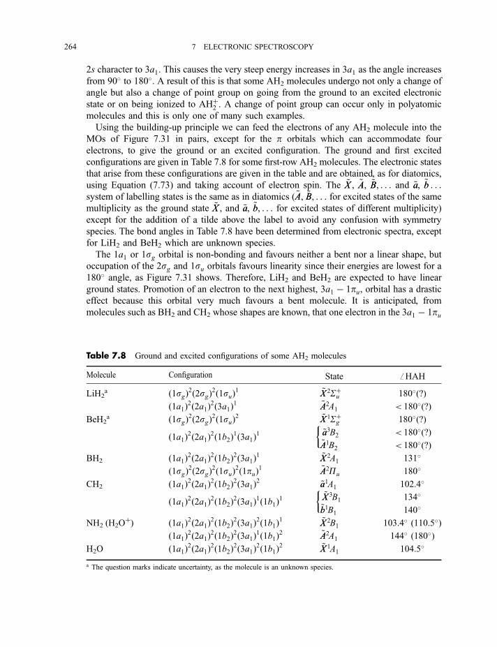
2s character to 3a1. This causes the very steep energy increases in 3a1 as the angle increases
from 90� to 180�. A result of this is that some AH2 molecules undergo not only a change of
angle but also a change of point group on going from the ground to an excited electronic
state or on being ionized to AHþ2 . A change of point group can occur only in polyatomic
molecules and this is only one of many such examples.
Using the building-up principle we can feed the electrons of any AH2 molecule into the
MOs of Figure 7.31 in pairs, except for the p orbitals which can accommodate four
electrons, to give the ground or an excited configuration. The ground and first excited
configurations are given in Table 7.8 for some first-row AH2 molecules. The electronic states
that arise from these configurations are given in the table and are obtained, as for diatomics,
using Equation (7.73) and taking account of electron spin. The ~XX , ~AA, ~BB, . . . and ~aa, ~bb . . .system of labelling states is the same as in diatomics ( ~AA, ~BB, . . . for excited states of the same
multiplicity as the ground state ~XX , and ~aa, ~bb, . . . for excited states of different multiplicity)
except for the addition of a tilde above the label to avoid any confusion with symmetry
species. The bond angles in Table 7.8 have been determined from electronic spectra, except
for LiH2 and BeH2 which are unknown species.
The 1a1 or 1sg orbital is non-bonding and favours neither a bent nor a linear shape, but
occupation of the 2sg and 1su orbitals favours linearity since their energies are lowest for a
180� angle, as Figure 7.31 shows. Therefore, LiH2 and BeH2 are expected to have linear
ground states. Promotion of an electron to the next highest, 3a1 � 1pu, orbital has a drasticeffect because this orbital very much favours a bent molecule. It is anticipated, from
molecules such as BH2 and CH2 whose shapes are known, that one electron in the 3a1 � 1pu
Table 7.8 Ground and excited configurations of some AH2 molecules
Molecule Configuration State ffHAHLiH2
a ð1sgÞ2ð2sgÞ2ð1suÞ1 ~XX 2Sþu 180�(?)ð1a1Þ2ð2a1Þ2ð3a1Þ1 ~AA2A1 < 180�(?)
BeH2a ð1sgÞ2ð2sgÞ2ð1suÞ2 ~XX 1Sþg 180�(?)
ð1a1Þ2ð2a1Þ2ð1b2Þ1ð3a1Þ1~aa3B2 < 180�(?)~AA1B2 < 180�(?)
BH2 ð1a1Þ2ð2a1Þ2ð1b2Þ2ð3a1Þ1 ~XX 2A1 131�
ð1sgÞ2ð2sgÞ2ð1suÞ2ð1puÞ1 ~AA2Pu 180�
CH2 ð1a1Þ2ð2a1Þ2ð1b2Þ2ð3a1Þ2 ~aa1A1 102.4�
ð1a1Þ2ð2a1Þ2ð1b2Þ2ð3a1Þ1ð1b1Þ1~XX 3B1 134�~bb1B1 140�
NH2 (H2Oþ) ð1a1Þ2ð2a1Þ2ð1b2Þ2ð3a1Þ2ð1b1Þ1 ~XX 2B1 103.4� (110.5�)
ð1a1Þ2ð2a1Þ2ð1b2Þ2ð3a1Þ1ð1b1Þ2 ~AA2A1 144� (180�)H2O ð1a1Þ2ð2a1Þ2ð1b2Þ2ð3a1Þ2ð1b1Þ2 ~XX 1A1 104.5�
a The question marks indicate uncertainty, as the molecule is an unknown species.
264 7 ELECTRONIC SPECTROSCOPY
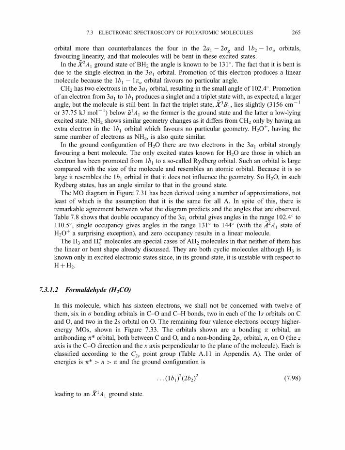
orbital more than counterbalances the four in the 2a1 � 2sg and 1b2 � 1su orbitals,
favouring linearity, and that molecules will be bent in these excited states.
In the ~XX 2A1 ground state of BH2 the angle is known to be 131�. The fact that it is bent isdue to the single electron in the 3a1 orbital. Promotion of this electron produces a linear
molecule because the 1b1 � 1pu orbital favours no particular angle.
CH2 has two electrons in the 3a1 orbital, resulting in the small angle of 102.4�. Promotion
of an electron from 3a1 to 1b1 produces a singlet and a triplet state with, as expected, a larger
angle, but the molecule is still bent. In fact the triplet state, ~XX 3B1, lies slightly (3156 cm71
or 37.75 kJ mol71) below ~aa1A1 so the former is the ground state and the latter a low-lying
excited state. NH2 shows similar geometry changes as it differs from CH2 only by having an
extra electron in the 1b1 orbital which favours no particular geometry. H2Oþ, having the
same number of electrons as NH2, is also quite similar.
In the ground configuration of H2O there are two electrons in the 3a1 orbital strongly
favouring a bent molecule. The only excited states known for H2O are those in which an
electron has been promoted from 1b1 to a so-called Rydberg orbital. Such an orbital is large
compared with the size of the molecule and resembles an atomic orbital. Because it is so
large it resembles the 1b1 orbital in that it does not influence the geometry. So H2O, in such
Rydberg states, has an angle similar to that in the ground state.
The MO diagram in Figure 7.31 has been derived using a number of approximations, not
least of which is the assumption that it is the same for all A. In spite of this, there is
remarkable agreement between what the diagram predicts and the angles that are observed.
Table 7.8 shows that double occupancy of the 3a1 orbital gives angles in the range 102.4� to110.5�, single occupancy gives angles in the range 131� to 144� (with the ~AA2A1 state of
H2Oþ a surprising exception), and zero occupancy results in a linear molecule.
The H3 and Hþ3 molecules are special cases of AH2 molecules in that neither of them has
the linear or bent shape already discussed. They are both cyclic molecules although H3 is
known only in excited electronic states since, in its ground state, it is unstable with respect to
HþH2.
7.3.1.2 Formaldehyde (H2CO)
In this molecule, which has sixteen electrons, we shall not be concerned with twelve of
them, six in s bonding orbitals in C–O and C–H bonds, two in each of the 1s orbitals on C
and O, and two in the 2s orbital on O. The remaining four valence electrons occupy higher-
energy MOs, shown in Figure 7.33. The orbitals shown are a bonding p orbital, an
antibonding p* orbital, both between C and O, and a non-bonding 2py orbital, n, on O (the z
axis is the C–O direction and the x axis perpendicular to the plane of the molecule). Each is
classified according to the C2v point group (Table A.11 in Appendix A). The order of
energies is p* > n > p and the ground configuration is
. . . ð1b1Þ2ð2b2Þ2 ð7:98Þ
leading to an ~XX 1A1 ground state.
7.3 ELECTRONIC SPECTROSCOPY OF POLYATOMIC MOLECULES 265
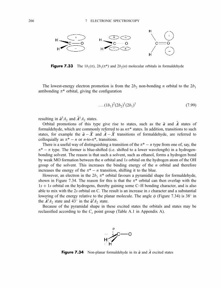
The lowest-energy electron promotion is from the 2b2 non-bonding n orbital to the 2b1antibonding p* orbital, giving the configuration
. . . ð1b1Þ2ð2b2Þ1ð2b1Þ1 ð7:99Þ
resulting in ~aa3A2 and ~AA1A2 states.
Orbital promotions of this type give rise to states, such as the ~aa and ~AA states of
formaldehyde, which are commonly referred to as np* states. In addition, transitions to such
states, for example the ~aa� ~XX and ~AA� ~XX transitions of formaldehyde, are referred to
colloquially as p*� n or n-to-p*, transitions.There is a useful way of distinguishing a transition of the p*� n type from one of, say, the
p*� p type. The former is blue-shifted (i.e. shifted to a lower wavelength) in a hydrogen-
bonding solvent. The reason is that such a solvent, such as ethanol, forms a hydrogen bond
by weak MO formation between the n orbital and 1s orbital on the hydrogen atom of the OH
group of the solvent. This increases the binding energy of the n orbital and therefore
increases the energy of the p*� n transition, shifting it to the blue.
However, an electron in the 2b1 p* orbital favours a pyramidal shape for formaldehyde,
shown in Figure 7.34. The reason for this is that the p* orbital can then overlap with the
1sþ 1s orbital on the hydrogens, thereby gaining some C–H bonding character, and is also
able to mix with the 2s orbital on C. The result is an increase in s character and a substantial
lowering of the energy relative to the planar molecule. The angle f (Figure 7.34) is 38� inthe ~AA1A2 state and 43� in the ~aa3A2 state.
Because of the pyramidal shape in these excited states the orbitals and states may be
reclassified according to the Cs point group (Table A.1 in Appendix A).
Figure 7.33 The 1b1ðpÞ, 2b1ðp*Þ and 2b2ðnÞ molecular orbitals in formaldehyde
Figure 7.34 Non-planar formaldehyde in its ~aa and ~AA excited states
266 7 ELECTRONIC SPECTROSCOPY
7.3.1.3 Benzene
In a molecule with electrons in p orbitals, such as formaldehyde, ethylene, buta-1,3-diene
and benzene, if we are concerned only with the ground state, or excited states obtained by
electron promotion within p-type MOs, an approximate MO method due to Huckel may be
useful.
The Huckel MO method is based on the LCAO method for diatomic molecules discussed
in Section 7.2.1. Extension of the LCAO method to polyatomic molecules gives a secular
determinant of the general type
H11 � E H12 � ES12 . . . H1n � ES1n
H12 � ES12 H22 � E . . . H2n � ES2n
..
. ... ..
.
H1n � ES1n H2n � ES2n . . . Hnn � E
¼ 0 ð7:100Þ
analogous to Equation (7.46) for a diatomic molecule, where the Hnn are Coulomb integrals,
Hmn (for m 6¼ n) are resonance integrals, Smn (for m 6¼ n) are overlap integrals, and E is the
orbital energy, as in Equation (7.46). This determinant may be abbreviated to
jHmn � ESmnj ¼ 0 ð7:101Þ
where Smn ¼ 1 when m ¼ n.
For p-electron systems Huckel made the following approximations:
1. Only electrons in p orbitals are considered, those in s orbitals being neglected. In a
molecule such as ethylene, with sufficiently high symmetry, the s–p separation is not an
approximation since the s and p MOs have different symmetry species and therefore
cannot mix. However, in a molecule of low symmetry such as but-1-ene
(CH3CH2CH¼CH2), the s and p MOs have the same symmetry species; in the Huckel
treatment, though, the s MOs are still neglected because they are assumed to be much
lower in energy than the p MOs.
2. It is assumed that, for m 6¼ n,
Smn ¼ 0 ð7:102Þ
implying no overlap of atomic orbitals even for nearest-neighbour atoms.
3. When m ¼ n the Coulomb integral Hnn is assumed to be the same for each atom and is
given the symbol a:
Hnn ¼ a ð7:103Þ
7.3 ELECTRONIC SPECTROSCOPY OF POLYATOMIC MOLECULES 267
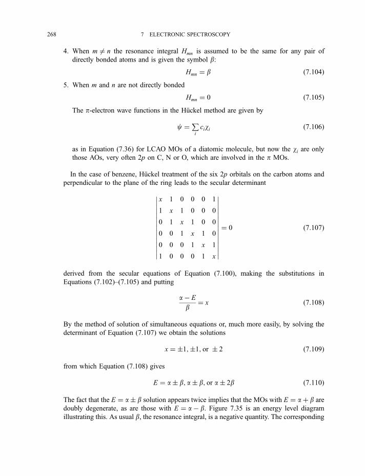
4. When m 6¼ n the resonance integral Hmn is assumed to be the same for any pair of
directly bonded atoms and is given the symbol b:
Hmn ¼ b ð7:104Þ5. When m and n are not directly bonded
Hmn ¼ 0 ð7:105ÞThe p-electron wave functions in the Huckel method are given by
c ¼Pi
ciwi ð7:106Þ
as in Equation (7.36) for LCAO MOs of a diatomic molecule, but now the wi are only
those AOs, very often 2p on C, N or O, which are involved in the p MOs.
In the case of benzene, Huckel treatment of the six 2p orbitals on the carbon atoms and
perpendicular to the plane of the ring leads to the secular determinant
x 1 0 0 0 1
1 x 1 0 0 0
0 1 x 1 0 0
0 0 1 x 1 0
0 0 0 1 x 1
1 0 0 0 1 x
¼ 0 ð7:107Þ
derived from the secular equations of Equation (7.100), making the substitutions in
Equations (7.102)–(7.105) and putting
a� E
b¼ x ð7:108Þ
By the method of solution of simultaneous equations or, much more easily, by solving the
determinant of Equation (7.107) we obtain the solutions
x ¼ �1;�1; or � 2 ð7:109Þ
from which Equation (7.108) gives
E ¼ a� b; a� b; or a� 2b ð7:110Þ
The fact that the E ¼ a� b solution appears twice implies that the MOs with E ¼ aþ b are
doubly degenerate, as are those with E ¼ a� b. Figure 7.35 is an energy level diagram
illustrating this. As usual b, the resonance integral, is a negative quantity. The corresponding
268 7 ELECTRONIC SPECTROSCOPY
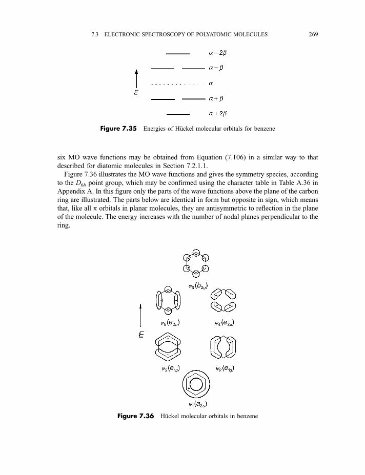
six MO wave functions may be obtained from Equation (7.106) in a similar way to that
described for diatomic molecules in Section 7.2.1.1.
Figure 7.36 illustrates the MO wave functions and gives the symmetry species, according
to the D6h point group, which may be confirmed using the character table in Table A.36 in
Appendix A. In this figure only the parts of the wave functions above the plane of the carbon
ring are illustrated. The parts below are identical in form but opposite in sign, which means
that, like all p orbitals in planar molecules, they are antisymmetric to reflection in the plane
of the molecule. The energy increases with the number of nodal planes perpendicular to the
ring.
Figure 7.35 Energies of Huckel molecular orbitals for benzene
Figure 7.36 Huckel molecular orbitals in benzene
7.3 ELECTRONIC SPECTROSCOPY OF POLYATOMIC MOLECULES 269
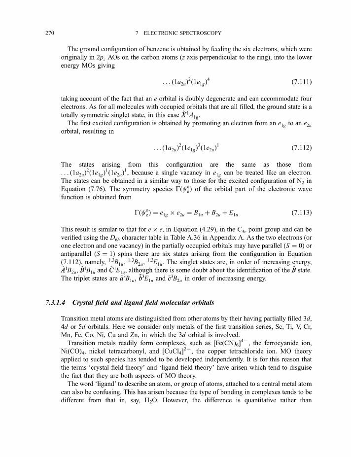
The ground configuration of benzene is obtained by feeding the six electrons, which were
originally in 2pz AOs on the carbon atoms (z axis perpendicular to the ring), into the lower
energy MOs giving
. . . ð1a2uÞ2ð1e1gÞ4 ð7:111Þ
taking account of the fact that an e orbital is doubly degenerate and can accommodate four
electrons. As for all molecules with occupied orbitals that are all filled, the ground state is a
totally symmetric singlet state, in this case ~XX 1A1g.
The first excited configuration is obtained by promoting an electron from an e1g to an e2uorbital, resulting in
. . . ð1a2uÞ2ð1e1gÞ3ð1e2uÞ1 ð7:112Þ
The states arising from this configuration are the same as those from
. . . ð1a2uÞ2ð1e1gÞ1ð1e2uÞ1, because a single vacancy in e1g can be treated like an electron.
The states can be obtained in a similar way to those for the excited configuration of N2 in
Equation (7.76). The symmetry species GðcoeÞ of the orbital part of the electronic wave
function is obtained from
GðcoeÞ ¼ e1g � e2u ¼ B1u þ B2u þ E1u ð7:113Þ
This result is similar to that for e� e, in Equation (4.29), in the C3v point group and can be
verified using the D6h character table in Table A.36 in Appendix A. As the two electrons (or
one electron and one vacancy) in the partially occupied orbitals may have parallel ðS ¼ 0Þ orantiparallel ðS ¼ 1Þ spins there are six states arising from the configuration in Equation
(7.112), namely, 1;3B1u ,1;3B2u,
1;3E1u. The singlet states are, in order of increasing energy,~AA1B2u, ~BB
1B1u and~CC1E1u, although there is some doubt about the identification of the ~BB state.
The triplet states are ~aa3B1u,~bb3E1u and ~cc3B2u in order of increasing energy.
7.3.1.4 Crystal field and ligand field molecular orbitals
Transition metal atoms are distinguished from other atoms by their having partially filled 3d,
4d or 5d orbitals. Here we consider only metals of the first transition series, Sc, Ti, V, Cr,
Mn, Fe, Co, Ni, Cu and Zn, in which the 3d orbital is involved.
Transition metals readily form complexes, such as [Fe(CN)6]47, the ferrocyanide ion,
Ni(CO)4, nickel tetracarbonyl, and [CuCl4]27, the copper tetrachloride ion. MO theory
applied to such species has tended to be developed independently. It is for this reason that
the terms ‘crystal field theory’ and ‘ligand field theory’ have arisen which tend to disguise
the fact that they are both aspects of MO theory.
The word ‘ligand’ to describe an atom, or group of atoms, attached to a central metal atom
can also be confusing. This has arisen because the type of bonding in complexes tends to be
different from that in, say, H2O. However, the difference is quantitative rather than
270 7 ELECTRONIC SPECTROSCOPY
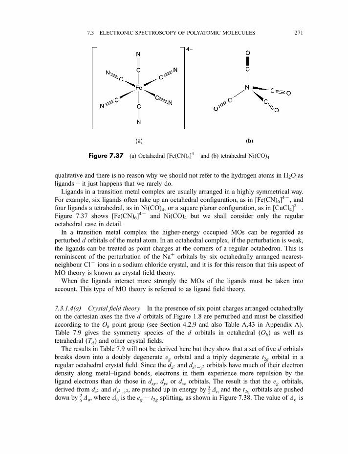
qualitative and there is no reason why we should not refer to the hydrogen atoms in H2O as
ligands – it just happens that we rarely do.
Ligands in a transition metal complex are usually arranged in a highly symmetrical way.
For example, six ligands often take up an octahedral configuration, as in [Fe(CN)6]47, and
four ligands a tetrahedral, as in Ni(CO)4, or a square planar configuration, as in [CuCl4]27.
Figure 7.37 shows [Fe(CN)6]47 and Ni(CO)4 but we shall consider only the regular
octahedral case in detail.
In a transition metal complex the higher-energy occupied MOs can be regarded as
perturbed d orbitals of the metal atom. In an octahedral complex, if the perturbation is weak,
the ligands can be treated as point charges at the corners of a regular octahedron. This is
reminiscent of the perturbation of the Naþ orbitals by six octahedrally arranged nearest-
neighbour Cl7 ions in a sodium chloride crystal, and it is for this reason that this aspect of
MO theory is known as crystal field theory.
When the ligands interact more strongly the MOs of the ligands must be taken into
account. This type of MO theory is referred to as ligand field theory.
7.3.1.4(a) Crystal field theory In the presence of six point charges arranged octahedrally
on the cartesian axes the five d orbitals of Figure 1.8 are perturbed and must be classified
according to the Oh point group (see Section 4.2.9 and also Table A.43 in Appendix A).
Table 7.9 gives the symmetry species of the d orbitals in octahedral ðOhÞ as well as
tetrahedral ðTdÞ and other crystal fields.
The results in Table 7.9 will not be derived here but they show that a set of five d orbitals
breaks down into a doubly degenerate eg orbital and a triply degenerate t2g orbital in a
regular octahedral crystal field. Since the dz2 and dx2�y2 orbitals have much of their electron
density along metal–ligand bonds, electrons in them experience more repulsion by the
ligand electrons than do those in dxy, dyz or dxz orbitals. The result is that the eg orbitals,
derived from dz2 and dx2�y2, are pushed up in energy by 35Do and the t2g orbitals are pushed
down by 25Do, where Do is the eg � t2g splitting, as shown in Figure 7.38. The value of Do is
Figure 7.37 (a) Octahedral [Fe(CN)6]47 and (b) tetrahedral Ni(CO)4
7.3 ELECTRONIC SPECTROSCOPY OF POLYATOMIC MOLECULES 271
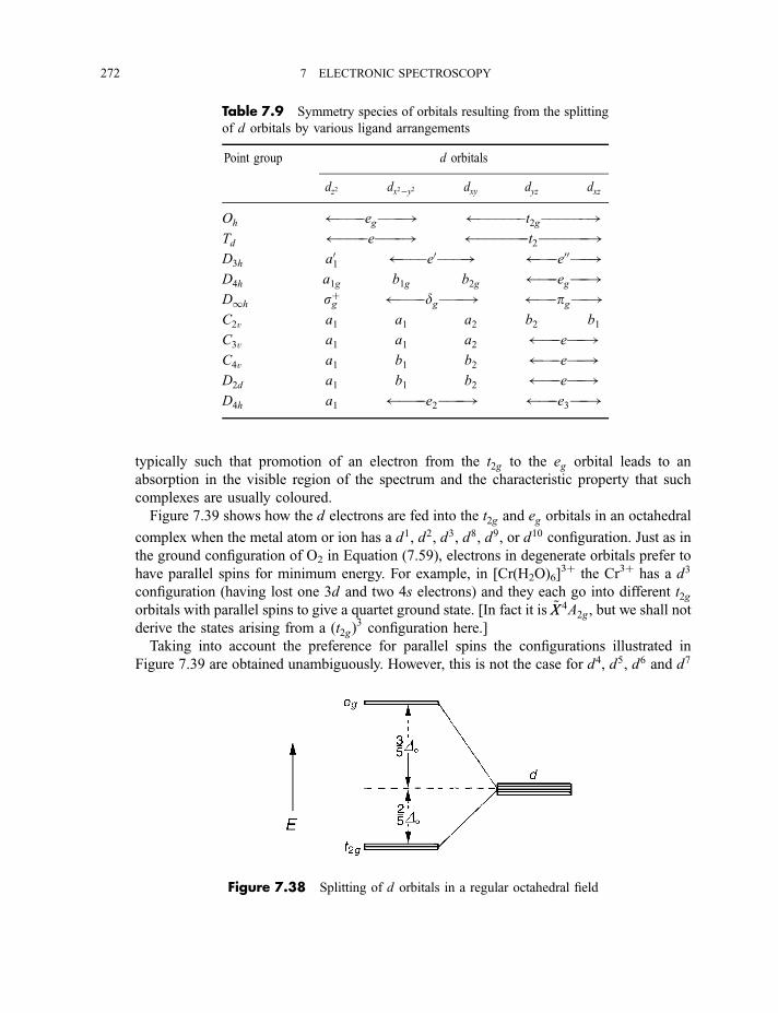
typically such that promotion of an electron from the t2g to the eg orbital leads to an
absorption in the visible region of the spectrum and the characteristic property that such
complexes are usually coloured.
Figure 7.39 shows how the d electrons are fed into the t2g and eg orbitals in an octahedral
complex when the metal atom or ion has a d1, d2, d3, d8, d9, or d10 configuration. Just as in
the ground configuration of O2 in Equation (7.59), electrons in degenerate orbitals prefer to
have parallel spins for minimum energy. For example, in [Cr(H2O)6]3þ the Cr3þ has a d3
configuration (having lost one 3d and two 4s electrons) and they each go into different t2gorbitals with parallel spins to give a quartet ground state. [In fact it is ~XX 4A2g, but we shall not
derive the states arising from a ðt2gÞ3 configuration here.]
Taking into account the preference for parallel spins the configurations illustrated in
Figure 7.39 are obtained unambiguously. However, this is not the case for d4, d5, d6 and d7
Table 7.9 Symmetry species of orbitals resulting from the splitting
of d orbitals by various ligand arrangements
Point group d orbitals
dz2 dx2�y2 dxy dyz dxz
Oh ����eg����! ������t2g������!Td ����e����! �������t2�������!D3h a01 ���e0���! ���e00���!D4h a1g b1g b2g ���eg���!D1h sþg ����dg����! ���pg���!C2v a1 a1 a2 b2 b1
C3v a1 a1 a2 ���e���!C4v a1 b1 b2 ���e���!D2d a1 b1 b2 ���e���!D4h a1 ����e2����! ���e3���!
Figure 7.38 Splitting of d orbitals in a regular octahedral field
272 7 ELECTRONIC SPECTROSCOPY
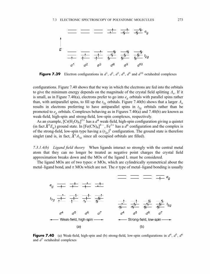
configurations. Figure 7.40 shows that the way in which the electrons are fed into the orbitals
to give the minimum energy depends on the magnitude of the crystal field splitting Do. If it
is small, as in Figure 7.40(a), electrons prefer to go into eg orbitals with parallel spins rather
than, with antiparallel spins, to fill up the t2g orbitals. Figure 7.40(b) shows that a larger Do
results in electrons preferring to have antiparallel spins in t2g orbitals rather than be
promoted to eg orbitals. Complexes behaving as in Figures 7.40(a) and 7.40(b) are known as
weak-field, high-spin and strong-field, low-spin complexes, respectively.
As an example, [Cr(H2O)6]2þ has a d4 weak-field, high-spin configuration giving a quintet
(in fact ~XX 5Eg) ground state. In [Fe(CN)6]47, Fe2þ has a d6 configuration and the complex is
of the strong-field, low-spin type having a ðt2gÞ6 configuration. The ground state is therefore
singlet (and is, in fact, ~XX 1A1g since all occupied orbitals are filled).
7.3.1.4(b) Ligand field theory When ligands interact so strongly with the central metal
atom that they can no longer be treated as negative point charges the crystal field
approximation breaks down and the MOs of the ligand L must be considered.
The ligand MOs are of two types: s MOs, which are cylindrically symmetrical about the
metal–ligand bond, and pMOs which are not. The s type of metal–ligand bonding is usually
Figure 7.39 Electron configurations in d1, d2, d3, d8, d9 and d10 octahedral complexes
Figure 7.40 (a) Weak-field, high-spin and (b) strong-field, low-spin configurations in d4, d5, d6
and d7 octahedral complexes
7.3 ELECTRONIC SPECTROSCOPY OF POLYATOMIC MOLECULES 273
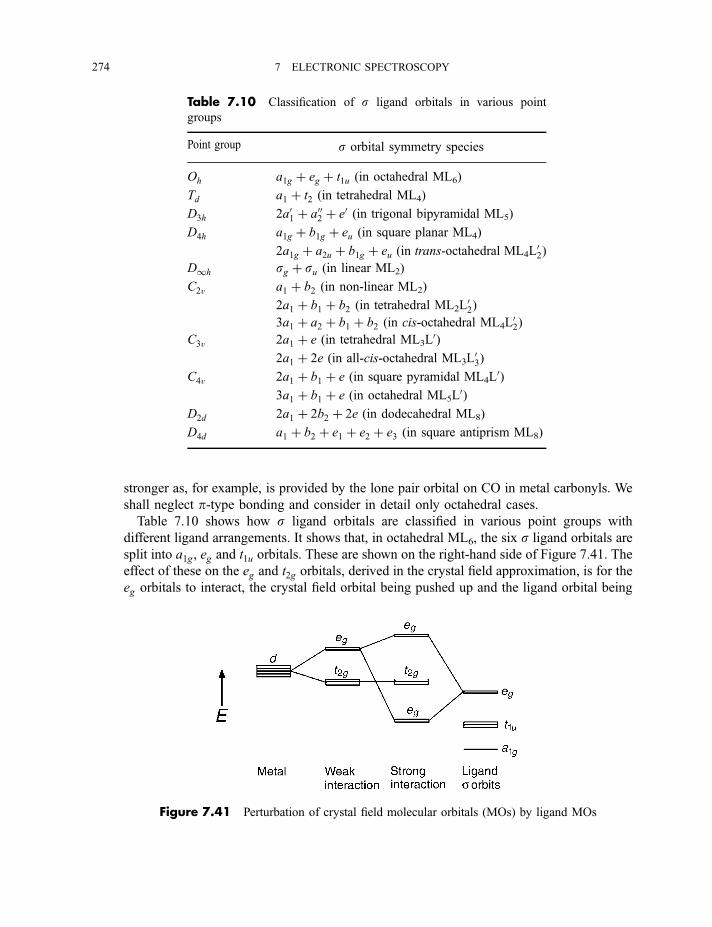
stronger as, for example, is provided by the lone pair orbital on CO in metal carbonyls. We
shall neglect p-type bonding and consider in detail only octahedral cases.
Table 7.10 shows how s ligand orbitals are classified in various point groups with
different ligand arrangements. It shows that, in octahedral ML6, the six s ligand orbitals are
split into a1g, eg and t1u orbitals. These are shown on the right-hand side of Figure 7.41. The
effect of these on the eg and t2g orbitals, derived in the crystal field approximation, is for the
eg orbitals to interact, the crystal field orbital being pushed up and the ligand orbital being
Figure 7.41 Perturbation of crystal field molecular orbitals (MOs) by ligand MOs
Table 7.10 Classification of s ligand orbitals in various point
groups
Point group s orbital symmetry species
Oh a1g þ eg þ t1u (in octahedral ML6)
Td a1 þ t2 (in tetrahedral ML4)
D3h 2a01 þ a002 þ e0 (in trigonal bipyramidal ML5)
D4h a1g þ b1g þ eu (in square planar ML4)
2a1g þ a2u þ b1g þ eu (in trans-octahedral ML4L02)
D1h sg þ su (in linear ML2)
C2v a1 þ b2 (in non-linear ML2)
2a1 þ b1 þ b2 (in tetrahedral ML2L02)
3a1 þ a2 þ b1 þ b2 (in cis-octahedral ML4L02)
C3v 2a1 þ e (in tetrahedral ML3L0)
2a1 þ 2e (in all-cis-octahedral ML3L03)
C4v 2a1 þ b1 þ e (in square pyramidal ML4L0)
3a1 þ b1 þ e (in octahedral ML5L0)
D2d 2a1 þ 2b2 þ 2e (in dodecahedral ML8)
D4d a1 þ b2 þ e1 þ e2 þ e3 (in square antiprism ML8)
274 7 ELECTRONIC SPECTROSCOPY
pushed down. The result, as shown in Figure 7.41, is to increase Do compared with its value
in the crystal field approximation. This increase in Do leads, in turn, to a tendency towards
low-spin rather than high-spin complexes, as in [Fe(CN)6]47.
7.3.1.4(c) Electronic transitions Both ground and excited electron configurations of
metal complexes often give rise to quite complex manifolds of states which we shall not
derive here. However, there is one simplifying factor which is extremely useful in
considering electronic spectra of transition metal complexes. All the higher-energy orbitals
which may be occupied, in regular octahedral complexes, are t2g or eg, whether we use the
crystal field or ligand field approach. Since the subscript g means ‘symmetric to inversion
through the centre of the molecule’ all states must be g also, since g multiplied by itself any
number of times (actually the number of times g orbitals are occupied) always gives g. So all
ground and excited states arising from t2g and eg occupancy are all g states. Just as in a
homonuclear diatomic molecule (see Equation 7.71), g–g transitions are forbidden.
However, transition metal complexes do absorb in the visible region, giving them a
characteristic colour. How can this happen if the transitions are forbidden? The answer is
that interaction may occur between the motion of the electrons and vibrational motions so
that some vibronic transitions are allowed (see Section 7.3.4.2b).
7.3.2 Electronic and vibronic selection rules
In the case of atoms (Section 7.1) a sufficient number of quantum numbers is available for us
to be able to express electronic selection rules entirely in terms of these quantum numbers.
For diatomic molecules (Section 7.2.3) we require, in addition to the quantum numbers
available, one or, for homonuclear diatomics, two symmetry properties (þ , 7 and g, u) of
the electronic wave function to obtain selection rules.
In non-linear polyatomic molecules the process of deterioration of quantum numbers
continues to such an extent that only the total electron spin quantum number S remains. The
selection rule
DS ¼ 0 ð7:114Þ
still applies, unless there is an atom with a high nuclear charge in the molecule. For example,
triplet–singlet transitions are extremely weak in benzene but much more intense in
iodobenzene.
For the orbital parts coe of the electronic wave functions of two electronic states the
selection rules depend entirely on symmetry properties. [In fact, the electronic selection
rules can also be obtained, from symmetry arguments only, for diatomic molecules and
atoms, using the D1h (or C1v) and Kh point groups, respectively; but it is more
straightforward to use quantum numbers when these are available.]
Electronic transitions mostly involve interaction between the molecule and the electric
component of the electromagnetic radiation (Section 2.1). The selection rules are, therefore,
7.3 ELECTRONIC SPECTROSCOPY OF POLYATOMIC MOLECULES 275
electric dipole selection rules analogous to those derived in Section 6.2.3.1 for infrared
vibrational transitions in polyatomic molecules.
The electronic transition intensity is proportional to jRej2, the square of the electronic
transition moment Re, where
Re ¼ðce0*mmc00e dte ð7:115Þ
which is similar to Equation (6.44) for an infrared vibrational transition. For an allowed
electronic transition, jRej 6¼ 0 and the symmetry requirement for this is
Gðc0eÞ � GðmÞ � Gðc00e Þ ¼ A ð7:116Þ
for a transition between non-degenerate states or
Gðc0eÞ � GðmÞ � Gðc00e Þ � A ð7:117Þ
where � means ‘contains’, for transitions between states where at least one of them is
degenerate. The symbol A stands for the totally symmetric species of the point group
concerned.
The components of Re along the cartesian axes are given by
Re;x ¼ðce0*mxc
00e dte
Re;y ¼ðce0*myc
00e dte
Re;z ¼ðce0*mzc
00e dte
9>>>>>>=>>>>>>;
ð7:118Þ
and, since
jRej2 ¼ ðRe;xÞ2 þ ðRe;yÞ2 þ ðRe;zÞ2 ð7:119Þ
the electronic transition is allowed if any of Re;x, Re;y or Re;z is non-zero. It follows that,
analogous to Equation (6.53), for a transition to be allowed
Gðc0eÞ � GðTxÞ � Gðc00e Þ ¼ A
and=or
Gðc0eÞ � GðTyÞ � Gðc00e Þ ¼ A
and=or
Gðc0eÞ � GðTzÞ � Gðc00e Þ ¼ A
9>>>>>>=>>>>>>;
ð7:120Þ
276 7 ELECTRONIC SPECTROSCOPY
for transitions between non-degenerate states (replace ¼ by � if a degenerate state is
involved), where Tx, etc., are translations along the corresponding axes.
If the product of two symmetry species is totally symmetric those species must be the
same. Therefore we can rewrite Equation (7.120) as
Gðc0eÞ � Gðc00e Þ ¼ GðTxÞ and=or GðTyÞ and=or GðTzÞ ð7:121Þ
or, if a degenerate state is involved, ¼ is replaced by �. This is the general selection rule for
a transition between two electronic states. If the lower state is the ground state of a molecule
with only filled orbitals, a so-called closed shell molecule, c00e is totally symmetric and
Equation (7.121) simplifies to
Gðc0eÞ ¼ GðTxÞ and=or GðTyÞ and=or GðTzÞ ð7:122Þ
This result is the same as the infrared vibrational selection rule in Equation (6.55).
If vibrations are excited in either the lower or the upper electronic state, or both, the
vibronic transition moment Rev, corresponding to the electronic transition moment Re in
Equation (7.115), is given by
Rev ¼ðcev0*mmc00ev dtev ð7:123Þ
where cev is a vibronic wave function. Following the same arguments as for electronic
transitions the selection rule analogous to that in Equation (7.121) is
Gðc0evÞ � Gðc00evÞ ¼ GðTxÞ and=or GðTyÞ and=or GðTzÞ ð7:124Þ
or, since
GðcevÞ ¼ GðceÞ � GðcvÞ ð7:125Þ
we obtain
Gðc0eÞ � Gðc0vÞ � Gðc00e Þ � Gðc00v Þ ¼ GðTxÞ and=or GðTyÞ and=or GðTzÞ ð7:126Þ
If a degenerate state is involved the ¼ is replaced by �. Very often either the same vibration
is excited in both states, in which case Gðc0vÞ ¼ Gðc00v Þ and the selection rule is the same as
the electronic selection rule, or no vibration is excited in the upper or lower state, resulting in
Gðc0vÞ or Gðc00v Þ being totally symmetric.
7.3 ELECTRONIC SPECTROSCOPY OF POLYATOMIC MOLECULES 277
7.3.3 Chromophores
The concept of a chromophore is analogous to that of a group vibration, discussed in Section
6.2.1. Just as the wavenumber of a group vibration is treated as transferable from one
molecule to another so is the wavenumber, or wavelength, at which an electronic transition
occurs in a particular group. Such a group is called a chromophore since it results in a
characteristic colour of the compound due to absorption of visible or, broadening the use of
the word ‘colour’, ultraviolet radiation.
The ethylenic group, , is an example. Whatever molecule contains the group,
such as H2C¼CH2, XHC¼CH2, X2C¼CH2, or cyclohexene, shows an intense absorption
system with a maximum intensity at about 180 nm. However, the group can act as a
chromophore only if it is not conjugated with any other p-electron system: for example,
buta-1,3-diene and benzene absorb at much longer wavelengths. Indeed, the benzene ring
itself can be treated as a chromophore showing a characteristic, fairly weak, absorption at
about 260 nm, like benzene itself (Section 7.3.1.3) and, say, phenylcyclohexane.
Similarly, the acetylenic group, �CC�, shows an intense absorption system at about
190 nm and the allylic group, , absorbs strongly at about 225 nm.
A transition involving a p*–n promotion is useful in identifying a chromophore as it gives
a characteristically weak absorption system which is usually to high wavelength of systems
due to p*–p promotions and may be interfered with by them. The aldehyde group, �CHO, isa useful chromophore showing a weak p*–n absorption system at about 280 nm, like
formaldehyde itself (Section 7.3.1.2). However, in a molecule such as benzaldehyde
(C6H5CHO), the aldehyde group is part of a conjugated p-electron system and can no longer
be treated as a chromophore.
Like group vibrations, the wavelength at which a chromophore absorbs can be employed
as an analytical tool, but a rather less useful one.
7.3.4 Vibrational coarse structure
As for diatomic molecules (Section 7.2.5.2) the vibrational (vibronic) transitions
accompanying an electronic transition fall into the general categories of progressions and
sequences, as illustrated in Figure 7.18. The main differences in a polyatomic molecule are
that there are 3N � 6 (or 3N � 5 for a linear molecule) vibrations – not just one – and that
some of these lower the symmetry of the molecule as they are non-totally symmetric.
7.3.4.1 Sequences
The most common type of sequence, one with Dv ¼ 0 shown in Figure 7.18, is always
allowed by symmetry because, whatever the symmetry of the vibration involved,
C C
C CC
278 7 ELECTRONIC SPECTROSCOPY
Gðc0vÞ ¼ Gðc00v Þ in Equation (7.126) and the product Gðc0vÞ � Gðc00v Þ is totally symmetric (or
contains the totally symmetric species). There may be several Dvi ¼ 0 sequences in various
vibrations i but only those vibrations with levels of a sufficiently low wavenumber to be
appreciably populated (see Equation 7.83) will form sequences. In a planar molecule the
lowest wavenumber vibrations are usually out-of-plane vibrations.
7.3.4.2 Progressions
7.3.4.2(a) Totally symmetric vibrations When the vibrations involved are totally
symmetric, progressions are formed for very much the same reasons as in a diatomic.
The Franck–Condon principle, described in Section 7.2.5.3, applies to each vibration
separately. If there is a geometry change from the lower to the upper electronic state in the
direction of one of the normal coordinates then the corresponding totally symmetric
vibration is excited and forms a progression. The length of the progression depends on the
size of the geometry change, as illustrated for a diatomic in Figure 7.22. Intensities along
each progression are given by Equation (7.88) where the vibrational overlap integral applies
to the vibration concerned.
One example of a long progression involves the CO stretching vibration in the~AA1A2 � ~XX 1A1 system of formaldehyde (see Section 7.3.1.2). Because the p*–n electron
promotion involves an electron going from a non-bonding orbital to one which is
antibonding between the C and O atoms, there is an increase of the C¼O bond length (from
1.21 A to 1.32 A) in the excited state and a long progression in the C¼O stretching
vibration results.
In the ~AA1B2u � ~XX 1A1g system of benzene (see Section 7.3.1.3) an electron is promoted
from an e1g orbital to a more antibonding e2u orbital, shown in Figure 7.36. The result is an
increase in all the C–C bond lengths (from 1.397 A to 1.434 A) in the excited state. This
gives rise to the long progression shown in the low resolution absorption spectrum in Figure
7.42, involving n1,14 the symmetrical ring-breathing vibration shown in Figure 6.13(f ).
In electronic spectroscopy of polyatomic molecules the system used for labelling vibronic
transitions employs N v0v00 to indicate a transition in which vibration N is excited with v00
quanta in the lower state and v0 quanta in the upper state. The pure electronic transition is
labelled 000. The system is very similar to the rather less often used system for pure
vibrational transitions described in Section 6.2.3.1.
In Figure 7.42 it is seen that the progression is built not on the 000 but on the 610 band. The
reason for this will become clear when we have seen, in the following section, how non-
totally symmetric vibrations may be active in an electronic band system.
7.3.4.2(b) Non-totally symmetric vibrations The general vibronic selection rule in
Equation (7.126) shows that many vibronic transitions involving one quantum of a non-
totally symmetric vibration are allowed. For example, consider a molecule such as
14 Using the Wilson numbering (see the bibliography to Chapter 6).
7.3 ELECTRONIC SPECTROSCOPY OF POLYATOMIC MOLECULES 279
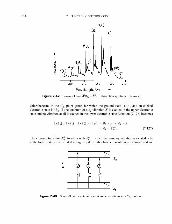
chlorobenzene in the C2v point group for which the ground state is 1A1 and an excited
electronic state is 1B2. If one quantum of a b2 vibration X is excited in the upper electronic
state and no vibration at all is excited in the lower electronic state Equation (7.126) becomes
Gðc0eÞ � Gðc0vÞ � Gðc00e Þ � Gðc00v Þ ¼ B2 � B2 � A1 � A1
¼ A1 ¼ GðTzÞ ð7:127Þ
The vibronic transition X 10 , together with X 0
1 in which the same b2 vibration is excited only
in the lower state, are illustrated in Figure 7.43. Both vibronic transitions are allowed and are
Figure 7.42 Low-resolution ~AA1B2u � ~XX 1A1g absorption spectrum of benzene
Figure 7.43 Some allowed electronic and vibronic transitions in a C2v molecule
280 7 ELECTRONIC SPECTROSCOPY
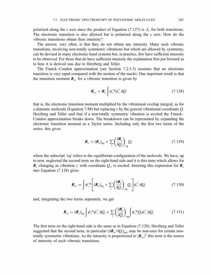
polarized along the z axis since the product of Equation (7.127) is A1 for both transitions.
The electronic transition is also allowed but is polarized along the y axis. How do the
vibronic transitions obtain their intensity?
The answer, very often, is that they do not obtain any intensity. Many such vibronic
transitions, involving non-totally symmetric vibrations but which are allowed by symmetry,
can be devised in many electronic band systems but, in practice, few have sufficient intensity
to be observed. For those that do have sufficient intensity the explanation first put forward as
to how it is derived was due to Herzberg and Teller.
The Franck–Condon approximation (see Section 7.2.5.3) assumes that an electronic
transition is very rapid compared with the motion of the nuclei. One important result is that
the transition moment Rev for a vibronic transition is given by
Rev ¼ Re
ðcv0*c00v dQ ð7:128Þ
that is, the electronic transition moment multiplied by the vibrational overlap integral, as for
a diatomic molecule (Equation 7.88) but replacing r by the general vibrational coordinate Q.
Herzberg and Teller said that if a non-totally symmetric vibration is excited the Franck–
Condon approximation breaks down. The breakdown can be represented by expanding the
electronic transition moment as a Taylor series. Including only the first two terms of the
series, this gives
Re ’ ðReÞeq þPi
@Re
@Qi
� �eq
Qi ð7:129Þ
where the subscript ‘eq’ refers to the equilibrium configuration of the molecule. We have, up
to now, neglected the second term on the right-hand side and it is this term which allows for
Re changing as vibration i, with coordinate Qi, is excited. Inserting this expression for Re
into Equation (7.128) gives
Rev ¼ðcv0* ðReÞeq þ
Pi
@Re
@Qi
� �eq
Qi
" #c00v dQi ð7:130Þ
and, integrating the two terms separately, we get
Rev ¼ ðReÞeqðcv0*c00v dQi þ
Pi
@Re
@Qi
� �eq
ðcv0*Qic
00v dQi ð7:131Þ
The first term on the right-hand side is the same as in Equation (7.128). Herzberg and Teller
suggested that the second term, in particular ð@Re=@QiÞeq, may be non-zero for certain non-
totally symmetric vibrations. As the intensity is proportional to jRevj2 this term is the source
of intensity of such vibronic transitions.
7.3 ELECTRONIC SPECTROSCOPY OF POLYATOMIC MOLECULES 281
Examples of vibronic transitions involving non-totally symmetric vibrations are in the~AA1B2 � ~XX 1A1 system of chlorobenzene, a C2v molecule. One b2 vibration n29, with a
wavenumber of 615 cm71 in the ~XX state and 523 cm71 in the ~AA state, is active in 2910 and
2901 bands similar to the case shown in Figure 7.43. There are 10 b2 vibrations in
chlorobenzene but the others are much less strongly active. The reason is that ð@Re=@Q29Þeqis much greater than the corresponding terms for all the other b2 vibrations.
The ~AA1B2 � ~XX 1A1 system of chlorobenzene is electronically allowed, since B2 ¼ GðTzÞ,which satisfies Equation (7.122). The 000 band, and progressions in totally symmetric
vibrations built on it, obtain their intensity in the usual way, through the first term on the
right-hand side of Equation (7.131).
The ~AA1B2u � ~XX 1A1g system of benzene (see Section 7.3.1.3), shown in Figure 7.42, is a
particularly interesting one. It is electronically forbidden, since B2u is not the symmetry
species of a translation (see Table A.36 in Appendix A); therefore ðReÞeq is zero and the 000band is not observed. All the intensity derives from the second term on the right-hand side of
Equation (7.131) and most of it through the e2g vibration n6. Since
B2u � e2g ¼ E1u ¼ GðTx; TyÞ ð7:132Þ
the 610 vibronic transition is allowed and is shown in Figure 7.42. The large value of
ð@R2=@Q6Þeq is responsible for the appreciable intensity of this band whereas the other three
e2g vibrations, n7, n8 and n9, are much less strongly active. The very weak 710 band is shown
in Figure 7.42 which shows also the 601 band, weakened by the Boltzmann factor, and the
position where the forbidden 000 band would be.
The ~AA1A2 � ~XX 1A1, p*–n system of formaldehyde (see Section 7.3.1.2) is also
electronically forbidden since A2 is not a symmetry species of a translation (see Table
A.11 in Appendix A). The main non-totally symmetric vibration which is active is n4, the b1out-of-plane bending vibration (see Worked example 4.1, page 90) in 410 and 401 transitions.
There are two further points of interest about this system of formaldehyde. First, as
mentioned in Section 7.3.1.2, the molecule is pyramidal in the ~AA state so that the potential
function for n4 is anharmonic in that state. It is W-shaped, rather like that for n2 in the groundelectronic state of ammonia in Figure 6.40, and the change of geometry from the ~XX to the ~AAstate leads to a progression in n4 in accordance with the Franck–Condon principle. The
second point of interest is that the 000 band is observed very weakly. The reason for this is
that, although the transition is forbidden by electric dipole selection rules, it is allowed by
magnetic dipole selection rules. A transition is magnetic dipole allowed if the excited state
symmetry species is that of a rotation of the molecule: in this case A2 ¼ GðRzÞ, as shown in
Table A.11 in Appendix A.
All the forbidden electronic transitions of regular octahedral transition metal complexes,
mentioned in Section 7.3.1.4, are induced by non-totally symmetric vibrations.
Although we have considered cases where ð@Re=@QiÞeq in Equation (7.131) may be quite
large for a non-totally symmetric vibration, a few cases are known where ð@Re=@QiÞeq is
appreciable for totally symmetric vibrations. In such cases the second term on the right-hand
side of Equation (7.131) provides an additional source of intensity for X 10 or X 0
1 vibronic
transitions when nX is totally symmetric.
282 7 ELECTRONIC SPECTROSCOPY
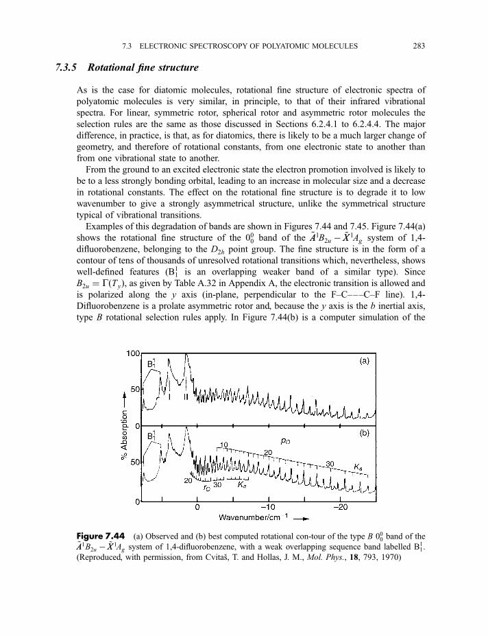
7.3.5 Rotational fine structure
As is the case for diatomic molecules, rotational fine structure of electronic spectra of
polyatomic molecules is very similar, in principle, to that of their infrared vibrational
spectra. For linear, symmetric rotor, spherical rotor and asymmetric rotor molecules the
selection rules are the same as those discussed in Sections 6.2.4.1 to 6.2.4.4. The major
difference, in practice, is that, as for diatomics, there is likely to be a much larger change of
geometry, and therefore of rotational constants, from one electronic state to another than
from one vibrational state to another.
From the ground to an excited electronic state the electron promotion involved is likely to
be to a less strongly bonding orbital, leading to an increase in molecular size and a decrease
in rotational constants. The effect on the rotational fine structure is to degrade it to low
wavenumber to give a strongly asymmetrical structure, unlike the symmetrical structure
typical of vibrational transitions.
Examples of this degradation of bands are shown in Figures 7.44 and 7.45. Figure 7.44(a)
shows the rotational fine structure of the 000 band of the ~AA1B2u � ~XX 1Ag system of 1,4-
difluorobenzene, belonging to the D2h point group. The fine structure is in the form of a
contour of tens of thousands of unresolved rotational transitions which, nevertheless, shows
well-defined features (B11 is an overlapping weaker band of a similar type). Since
B2u ¼ GðTyÞ, as given by Table A.32 in Appendix A, the electronic transition is allowed and
is polarized along the y axis (in-plane, perpendicular to the F–C–––C–F line). 1,4-
Difluorobenzene is a prolate asymmetric rotor and, because the y axis is the b inertial axis,
type B rotational selection rules apply. In Figure 7.44(b) is a computer simulation of the
Figure 7.44 (a) Observed and (b) best computed rotational con-tour of the type B 000 band of the~AA1B2u � ~XX 1Ag system of 1,4-difluorobenzene, with a weak overlapping sequence band labelled B1
1.
(Reproduced, with permission, from Cvitas, T. and Hollas, J. M., Mol. Phys., 18, 793, 1970)
7.3 ELECTRONIC SPECTROSCOPY OF POLYATOMIC MOLECULES 283
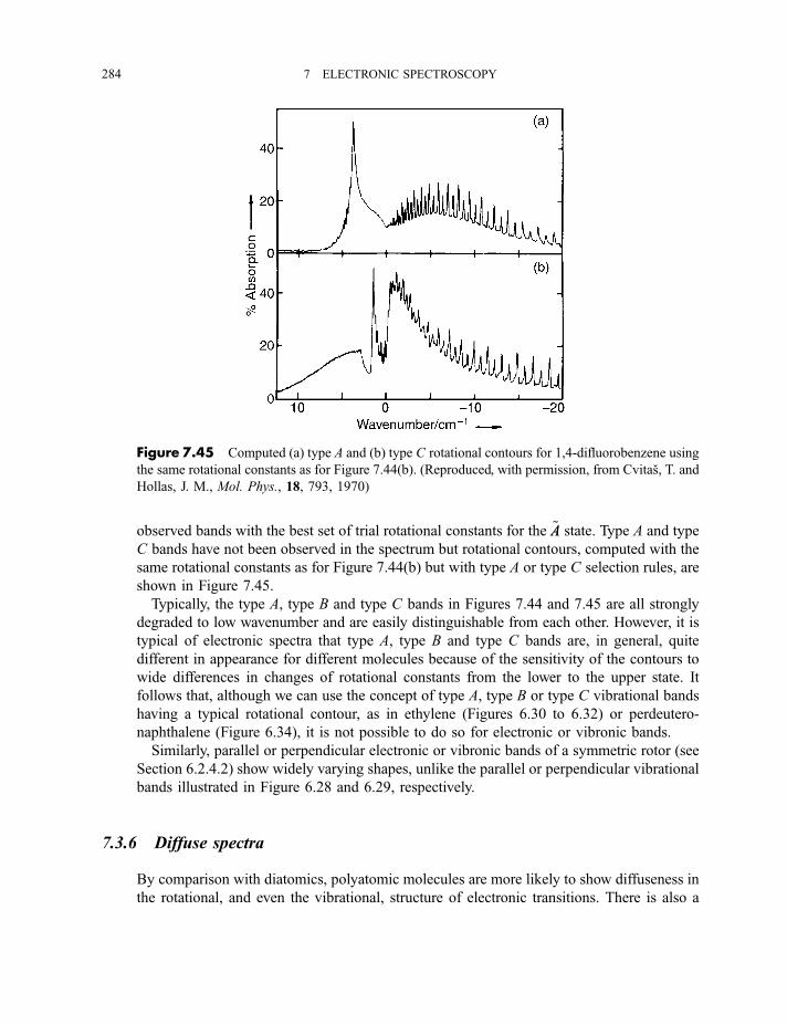
observed bands with the best set of trial rotational constants for the ~AA state. Type A and type
C bands have not been observed in the spectrum but rotational contours, computed with the
same rotational constants as for Figure 7.44(b) but with type A or type C selection rules, are
shown in Figure 7.45.
Typically, the type A, type B and type C bands in Figures 7.44 and 7.45 are all strongly
degraded to low wavenumber and are easily distinguishable from each other. However, it is
typical of electronic spectra that type A, type B and type C bands are, in general, quite
different in appearance for different molecules because of the sensitivity of the contours to
wide differences in changes of rotational constants from the lower to the upper state. It
follows that, although we can use the concept of type A, type B or type C vibrational bands
having a typical rotational contour, as in ethylene (Figures 6.30 to 6.32) or perdeutero-
naphthalene (Figure 6.34), it is not possible to do so for electronic or vibronic bands.
Similarly, parallel or perpendicular electronic or vibronic bands of a symmetric rotor (see
Section 6.2.4.2) show widely varying shapes, unlike the parallel or perpendicular vibrational
bands illustrated in Figure 6.28 and 6.29, respectively.
7.3.6 Diffuse spectra
By comparison with diatomics, polyatomic molecules are more likely to show diffuseness in
the rotational, and even the vibrational, structure of electronic transitions. There is also a
Figure 7.45 Computed (a) type A and (b) type C rotational contours for 1,4-difluorobenzene using
the same rotational constants as for Figure 7.44(b). (Reproduced, with permission, from Cvitas, T. and
Hollas, J. M., Mol. Phys., 18, 793, 1970)
284 7 ELECTRONIC SPECTROSCOPY
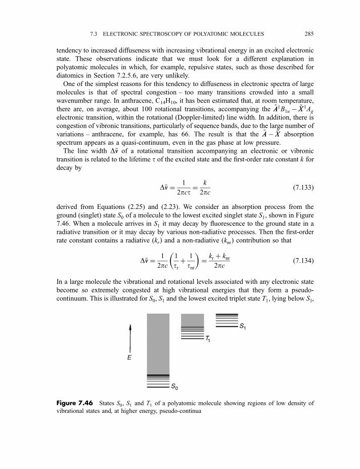
tendency to increased diffuseness with increasing vibrational energy in an excited electronic
state. These observations indicate that we must look for a different explanation in
polyatomic molecules in which, for example, repulsive states, such as those described for
diatomics in Section 7.2.5.6, are very unlikely.
One of the simplest reasons for this tendency to diffuseness in electronic spectra of large
molecules is that of spectral congestion – too many transitions crowded into a small
wavenumber range. In anthracene, C14H10, it has been estimated that, at room temperature,
there are, on average, about 100 rotational transitions, accompanying the ~AA1B1u � ~XX 1Ag
electronic transition, within the rotational (Doppler-limited) line width. In addition, there is
congestion of vibronic transitions, particularly of sequence bands, due to the large number of
variations – anthracene, for example, has 66. The result is that the ~AA� ~XX absorption
spectrum appears as a quasi-continuum, even in the gas phase at low pressure.
The line width D~nn of a rotational transition accompanying an electronic or vibronic
transition is related to the lifetime t of the excited state and the first-order rate constant k for
decay by
D~nn ¼ 1
2pct¼ k
2pcð7:133Þ
derived from Equations (2.25) and (2.23). We consider an absorption process from the
ground (singlet) state S0 of a molecule to the lowest excited singlet state S1, shown in Figure
7.46. When a molecule arrives in S1 it may decay by fluorescence to the ground state in a
radiative transition or it may decay by various non-radiative processes. Then the first-order
rate constant contains a radiative ðkrÞ and a non-radiative ðknrÞ contribution so that
D~nn ¼ 1
2pc1
trþ 1
tnr
� �¼ kr þ knr
2pcð7:134Þ
In a large molecule the vibrational and rotational levels associated with any electronic state
become so extremely congested at high vibrational energies that they form a pseudo-
continuum. This is illustrated for S0, S1 and the lowest excited triplet state T1, lying below S1,
Figure 7.46 States S0, S1 and T1 of a polyatomic molecule showing regions of low density of
vibrational states and, at higher energy, pseudo-continua
7.3 ELECTRONIC SPECTROSCOPY OF POLYATOMIC MOLECULES 285
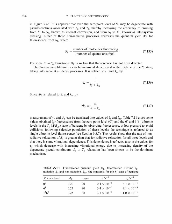
in Figure 7.46. It is apparent that even the zero-point level of S1 may be degenerate with
pseudo-continua associated with S0 and T1, thereby increasing the efficiency of crossing
from S1 to S0, known as internal conversion, and from S1 to T1, known as inter-system
crossing. Either of these non-radiative processes decreases the quantum yield FF for
fluorescence from S1, where
FF ¼number of molecules fluorescing
number of quanta absorbedð7:135Þ
For some S1 � S0 transitions, FF is so low that fluorescence has not been detected.
The fluorescence lifetime tF can be measured directly and is the lifetime of the S1 state,
taking into account all decay processes. It is related to kr and knr by
tF ¼1
kr þ knrð7:136Þ
Since FF is related to kr and knr by
FF ¼kr
kr þ knrð7:137Þ
measurement of tF and FF can be translated into values of kr and knr. Table 7.11 gives some
values obtained for fluorescence from the zero-point level (00) and the 61 and 1161 vibronic
levels in the S1 ð ~AA1B2uÞ state of benzene by observing fluorescence, at low pressure to avoid
collisions, following selective population of these levels: the technique is referred to as
single vibronic level fluorescence (see Section 9.3.7). The results show that the rate of non-
radiative relaxation of S1 is greater than that for radiative relaxation for all three levels and
that there is some vibrational dependence. This dependence is reflected also in the values for
tF which decrease with increasing vibrational energy due to increasing density of the
degenerate pseudo-continuum. S1 to T1 relaxation has been shown to be the dominant
mechanism.
Table 7.11 Fluorescence quantum yield FF, fluorescence lifetime tF,radiative, kr, and non-radiative, knr; rate constants for the S1 state of benzene
Vibronic level FF tF=ns kr=s71 knr=s
71
00 0.22 90 2.46 1076 8.76 1076
61 0.27 80 3.46 1076 9.16 1076
1161 0.25 68 3.76 1076 11.06 1076
286 7 ELECTRONIC SPECTROSCOPY
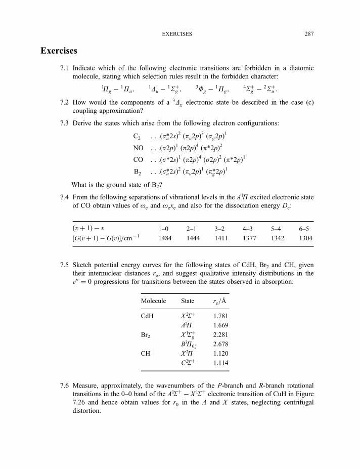
Exercises
7.1 Indicate which of the following electronic transitions are forbidden in a diatomic
molecule, stating which selection rules result in the forbidden character:
1Pg � 1Pu;1Du � 1Sþg ;
3Fg � 1Pg;4Sþg � 2Sþu :
7.2 How would the components of a 3Dg electronic state be described in the case (c)
coupling approximation?
7.3 Derive the states which arise from the following electron configurations:
C2 : : :ðsu*2sÞ2 ðpu2pÞ3 ðsg2pÞ1
NO : : :ðs2pÞ1 ðp2pÞ4 ðp*2pÞ2CO : : :ðs*2sÞ1 ðp2pÞ4 ðs2pÞ2 ðp*2pÞ1B2 : : :ðsu*2sÞ2 ðpu2pÞ1 ðpg*2pÞ1
What is the ground state of B2?
7.4 From the following separations of vibrational levels in the A1P excited electronic state
of CO obtain values of oe and oexe and also for the dissociation energy De:
ðvþ 1Þ � v 1–0 2–1 3–2 4–3 5–4 6–5
½Gðvþ 1Þ � GðvÞ�=cm71 1484 1444 1411 1377 1342 1304
7.5 Sketch potential energy curves for the following states of CdH, Br2 and CH, given
their internuclear distances re, and suggest qualitative intensity distributions in the
v00 ¼ 0 progressions for transitions between the states observed in absorption:
Molecule State re=A
CdH X 2Sþ 1.781
A2P 1.669
Br2 X 1Sþg 2.281
B3P0þu 2.678
CH X 2P 1.120
C2Sþ 1.114
7.6 Measure, approximately, the wavenumbers of the P-branch and R-branch rotational
transitions in the 0–0 band of the A1Sþ � X 1Sþ electronic transition of CuH in Figure
7.26 and hence obtain values for r0 in the A and X states, neglecting centrifugal
distortion.
EXERCISES 287
7.7 Discuss, briefly, the valence molecular orbitals of AlH2 and the shape of the molecule
in the ground and first excited singlet states.
7.8 For formaldehyde give the lowest MO configuration resulting from a p*–p promotion
and deduce the resulting states.
7.9 Show how the determinant Equation (7.107) gives the results in Equation (7.109).
7.10 Write down the crystal field orbital configurations of the following transition metal
complexes: [Cu(H2O)6]2þ, [V(H2O)6]
3þ, [Mn(H2O)6]2þ–high spin, [Co(NH3)6]
3þ–low spin. Explain why [Mn(H2O)6]
2þ is colourless.
7.11 A 1B3g � 1Ag electronic transition in a molecule belonging to the D2h point group is
forbidden. What are the possible symmetry species of a vibration X which would
result in the X10 and X0
1 transitions being allowed?
7.12 Show that the following electronic transitions:
(a) 1E � 1A1 in methyl fluoride;
(b) 1A002 � 1A01 in 1,3,5-trichlorobenzene;
(c) 1B2 � 1A1 in allene (CH2¼C¼CH2);
are allowed, determine the direction of the transition moment and state the rotational
selection rules that apply.
Bibliography
Candler, C. (1964) Atomic Spectra, Hilger and Watts, London.
Condon, E. U. and Shortley, G. H. (1953) The Theory of Atomic Spectra, Cambridge University Press,
Cambridge.
Coulson, C. A. (1961) Valence, Oxford University Press, Oxford.
Coulson, C. A. and McWeeney, R. (1979) Coulson’s Valence, Oxford University Press, Oxford.
Herzberg, G. (1944) Atomic Spectra and Atomic Structure, Dover, New York.
Herzberg, G. (1989) Spectra of Diatomic Molecules, Krieger, Florida.
Herzberg, G. (1991) Electronic Spectra and Electronic Structure of Polyatomic Molecules, Krieger,
Florida.
Huber, K. P. and Herzberg, G. (1979) Constants of Diatomic Molecules, Van Nostrand Reinhold,
New York.
Kettle, S. F. A. (1995) Symmetry and Structure, 2nd edn, John Wiley, Chichester.
King, G. W. (1964) Spectroscopy and Molecular Structure, Holt, Rinehart and Winston, New York.
Kuhn, H. G. (1969) Atomic Spectra, Longman, London.
Murrell, J. N., Kettle, S. F. A. and Tedder, J. M. (1970) Valence Theory. 2nd edn, John Wiley,
Chichester.
Murrell, J. N., Kettle, S. F. A. and Tedder, J. M. (1985) The Chemical Bond. 2nd edn, John Wiley,
Chichester.
Softley, T. P. (1994) Atomic Spectra, Oxford University Press, Oxford.
Steinfeld, J. I. (1985) Molecules and Radiation. 2nd edn, MIT Press, Cambridge, MA.
Walsh, A. D. (1953) J. Chem. Soc., 1953, 2260–2317.
288 7 ELECTRONIC SPECTROSCOPY
8Photoelectron and RelatedSpectroscopies
8.1 Photoelectron spectroscopy
Photoelectron spectroscopy involves the ejection of electrons from atoms or molecules
following bombardment by monochromatic photons. The ejected electrons are called
photoelectrons and were mentioned, in the context of the photoelectric effect, in Section 1.2.
The effect was observed originally on surfaces of easily ionizable metals, such as the alkali
metals. Bombardment of the surface with photons of tunable frequency does not produce
any photoelectrons until the threshold frequency is reached (see Figure 1.2). At this
frequency, nt, the photon energy is just sufficient to overcome the work function F of the
metal, so that
hnt ¼ F ð8:1Þ
At higher frequencies the excess energy of the photons is converted into kinetic energy of
the photoelectrons
hn ¼ Fþ 12mev2 ð8:2Þ
where me and v are their mass and velocity.
Work functions of alkali metal surfaces are only a few electronvolts1 so that the energy of
near ultraviolet radiation is sufficient to produce ionization.
Photoelectron spectroscopy is a simple extension of the photoelectric effect involving the
use of higher-energy incident photons and applied to the study not only of solid surfaces but
also of samples in the gas phase. Equations (8.1) and (8.2) still apply but, for gas-phase
measurements in particular, the work function is usually replaced by the ionization energy
I ;2 so that Equation (8.2) becomes
hn ¼ I þ 12mev2 ð8:3Þ
1 1 eV¼ 96.485 kJ mol71¼ 8065.54 cm71.2 This is often referred to as the ionization potential, but since Equation (8.3) shows that I has
dimensions of energy, the term ionization energy is to be preferred.
289
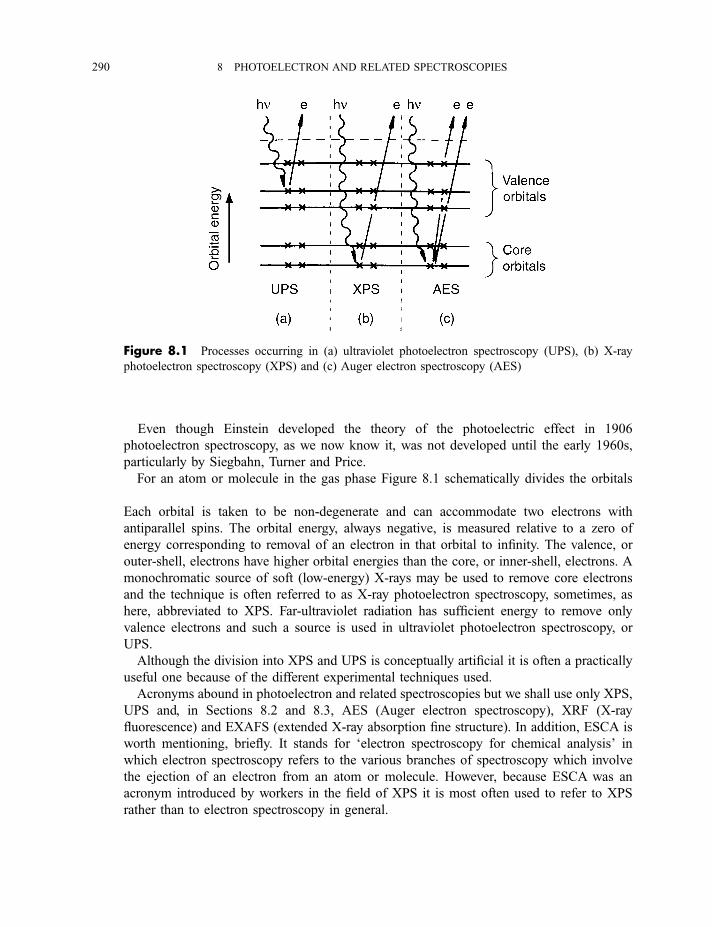
Even though Einstein developed the theory of the photoelectric effect in 1906
photoelectron spectroscopy, as we now know it, was not developed until the early 1960s,
particularly by Siegbahn, Turner and Price.
For an atom or molecule in the gas phase Figure 8.1 schematically divides the orbitals
[atomic orbitals (AOs) or molecular orbitals (MOs)] into core orbitals and valence orbitals.
Each orbital is taken to be non-degenerate and can accommodate two electrons with
antiparallel spins. The orbital energy, always negative, is measured relative to a zero of
energy corresponding to removal of an electron in that orbital to infinity. The valence, or
outer-shell, electrons have higher orbital energies than the core, or inner-shell, electrons. A
monochromatic source of soft (low-energy) X-rays may be used to remove core electrons
and the technique is often referred to as X-ray photoelectron spectroscopy, sometimes, as
here, abbreviated to XPS. Far-ultraviolet radiation has sufficient energy to remove only
valence electrons and such a source is used in ultraviolet photoelectron spectroscopy, or
UPS.
Although the division into XPS and UPS is conceptually artificial it is often a practically
useful one because of the different experimental techniques used.
Acronyms abound in photoelectron and related spectroscopies but we shall use only XPS,
UPS and, in Sections 8.2 and 8.3, AES (Auger electron spectroscopy), XRF (X-ray
fluorescence) and EXAFS (extended X-ray absorption fine structure). In addition, ESCA is
worth mentioning, briefly. It stands for ‘electron spectroscopy for chemical analysis’ in
which electron spectroscopy refers to the various branches of spectroscopy which involve
the ejection of an electron from an atom or molecule. However, because ESCA was an
acronym introduced by workers in the field of XPS it is most often used to refer to XPS
rather than to electron spectroscopy in general.
Figure 8.1 Processes occurring in (a) ultraviolet photoelectron spectroscopy (UPS), (b) X-ray
photoelectron spectroscopy (XPS) and (c) Auger electron spectroscopy (AES)
290 8 PHOTOELECTRON AND RELATED SPECTROSCOPIES
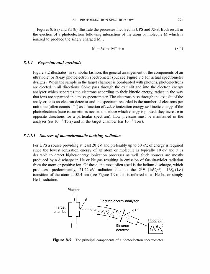
Figures 8.1(a) and 8.1(b) illustrate the processes involved in UPS and XPS. Both result in
the ejection of a photoelectron following interaction of the atom or molecule M which is
ionized to produce the singly charged Mþ.
Mþ hn! Mþ þ e ð8:4Þ
8.1.1 Experimental methods
Figure 8.2 illustrates, in symbolic fashion, the general arrangement of the components of an
ultraviolet or X-ray photoelectron spectrometer (but see Figure 8.5 for actual spectrometer
designs). When the sample in the target chamber is bombarded with photons, photoelectrons
are ejected in all directions. Some pass through the exit slit and into the electron energy
analyser which separates the electrons according to their kinetic energy, rather in the way
that ions are separated in a mass spectrometer. The electrons pass through the exit slit of the
analyser onto an electron detector and the spectrum recorded is the number of electrons per
unit time (often counts s71) as a function of either ionization energy or kinetic energy of the
photoelectrons (care is sometimes needed to deduce which energy is plotted: they increase in
opposite directions for a particular spectrum). Low pressure must be maintained in the
analyser (ca 1075 Torr) and in the target chamber (ca 1072 Torr).
8.1.1.1 Sources of monochromatic ionizing radiation
For UPS a source providing at least 20 eV, and preferably up to 50 eV, of energy is required
since the lowest ionization energy of an atom or molecule is typically 10 eV and it is
desirable to detect higher-energy ionization processes as well. Such sources are mostly
produced by a discharge in He or Ne gas resulting in emission of far-ultraviolet radiation
from the atom or positive ion. Of these, the most often used is the helium discharge, which
produces, predominantly, 21.22 eV radiation due to the 21P1 ð1s12p1Þ � 11S0 ð1s2Þtransition of the atom at 58.4 nm (see Figure 7.9): this is referred to as He Ia, or simply
He I, radiation.
Figure 8.2 The principal components of a photoelectron spectrometer
8.1 PHOTOELECTRON SPECTROSCOPY 291
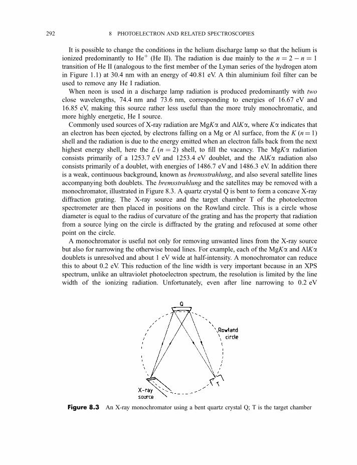
It is possible to change the conditions in the helium discharge lamp so that the helium is
ionized predominantly to Heþ (He II). The radiation is due mainly to the n ¼ 2� n ¼ 1
transition of He II (analogous to the first member of the Lyman series of the hydrogen atom
in Figure 1.1) at 30.4 nm with an energy of 40.81 eV. A thin aluminium foil filter can be
used to remove any He I radiation.
When neon is used in a discharge lamp radiation is produced predominantly with two
close wavelengths, 74.4 nm and 73.6 nm, corresponding to energies of 16.67 eV and
16.85 eV, making this source rather less useful than the more truly monochromatic, and
more highly energetic, He I source.
Commonly used sources of X-ray radiation are MgKa and AlKa, where Ka indicates that
an electron has been ejected, by electrons falling on a Mg or Al surface, from the K (n¼ 1)
shell and the radiation is due to the energy emitted when an electron falls back from the next
highest energy shell, here the L ðn ¼ 2Þ shell, to fill the vacancy. The MgKa radiation
consists primarily of a 1253.7 eV and 1253.4 eV doublet, and the AlKa radiation also
consists primarily of a doublet, with energies of 1486.7 eV and 1486.3 eV. In addition there
is a weak, continuous background, known as bremsstrahlung, and also several satellite lines
accompanying both doublets. The bremsstrahlung and the satellites may be removed with a
monochromator, illustrated in Figure 8.3. A quartz crystal Q is bent to form a concave X-ray
diffraction grating. The X-ray source and the target chamber T of the photoelectron
spectrometer are then placed in positions on the Rowland circle. This is a circle whose
diameter is equal to the radius of curvature of the grating and has the property that radiation
from a source lying on the circle is diffracted by the grating and refocused at some other
point on the circle.
A monochromator is useful not only for removing unwanted lines from the X-ray source
but also for narrowing the otherwise broad lines. For example, each of the MgKa and AlKadoublets is unresolved and about 1 eV wide at half-intensity. A monochromator can reduce
this to about 0.2 eV. This reduction of the line width is very important because in an XPS
spectrum, unlike an ultraviolet photoelectron spectrum, the resolution is limited by the line
width of the ionizing radiation. Unfortunately, even after line narrowing to 0.2 eV
Figure 8.3 An X-ray monochromator using a bent quartz crystal Q; T is the target chamber
292 8 PHOTOELECTRON AND RELATED SPECTROSCOPIES
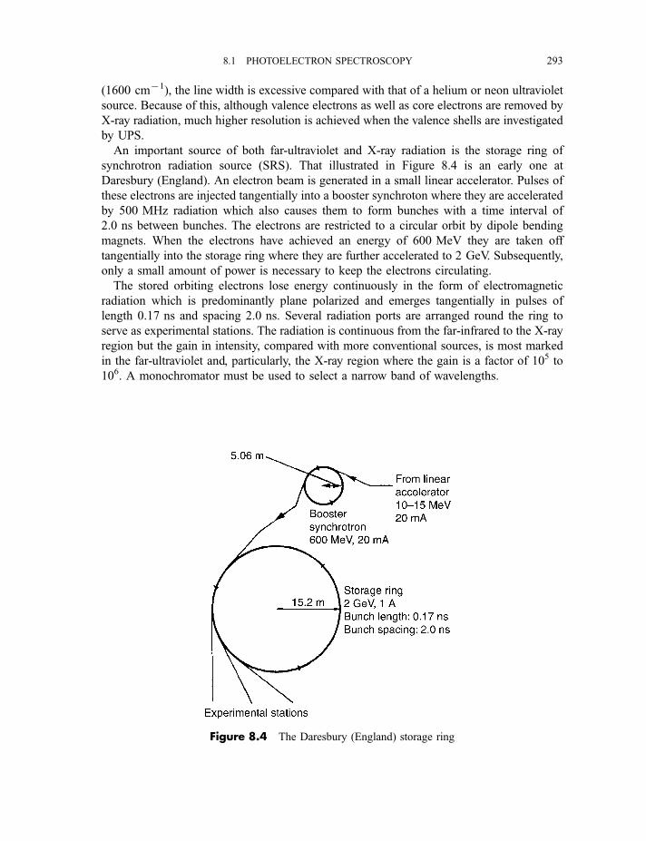
(1600 cm71), the line width is excessive compared with that of a helium or neon ultraviolet
source. Because of this, although valence electrons as well as core electrons are removed by
X-ray radiation, much higher resolution is achieved when the valence shells are investigated
by UPS.
An important source of both far-ultraviolet and X-ray radiation is the storage ring of
synchrotron radiation source (SRS). That illustrated in Figure 8.4 is an early one at
Daresbury (England). An electron beam is generated in a small linear accelerator. Pulses of
these electrons are injected tangentially into a booster synchroton where they are accelerated
by 500 MHz radiation which also causes them to form bunches with a time interval of
2.0 ns between bunches. The electrons are restricted to a circular orbit by dipole bending
magnets. When the electrons have achieved an energy of 600 MeV they are taken off
tangentially into the storage ring where they are further accelerated to 2 GeV. Subsequently,
only a small amount of power is necessary to keep the electrons circulating.
The stored orbiting electrons lose energy continuously in the form of electromagnetic
radiation which is predominantly plane polarized and emerges tangentially in pulses of
length 0.17 ns and spacing 2.0 ns. Several radiation ports are arranged round the ring to
serve as experimental stations. The radiation is continuous from the far-infrared to the X-ray
region but the gain in intensity, compared with more conventional sources, is most marked
in the far-ultraviolet and, particularly, the X-ray region where the gain is a factor of 105 to
106. A monochromator must be used to select a narrow band of wavelengths.
Figure 8.4 The Daresbury (England) storage ring
8.1 PHOTOELECTRON SPECTROSCOPY 293
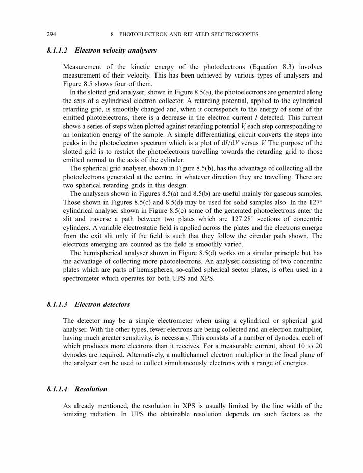
8.1.1.2 Electron velocity analysers
Measurement of the kinetic energy of the photoelectrons (Equation 8.3) involves
measurement of their velocity. This has been achieved by various types of analysers and
Figure 8.5 shows four of them.
In the slotted grid analyser, shown in Figure 8.5(a), the photoelectrons are generated along
the axis of a cylindrical electron collector. A retarding potential, applied to the cylindrical
retarding grid, is smoothly changed and, when it corresponds to the energy of some of the
emitted photoelectrons, there is a decrease in the electron current I detected. This current
shows a series of steps when plotted against retarding potential V, each step corresponding to
an ionization energy of the sample. A simple differentiating circuit converts the steps into
peaks in the photoelectron spectrum which is a plot of dI=dV versus V. The purpose of the
slotted grid is to restrict the photoelectrons travelling towards the retarding grid to those
emitted normal to the axis of the cylinder.
The spherical grid analyser, shown in Figure 8.5(b), has the advantage of collecting all the
photoelectrons generated at the centre, in whatever direction they are travelling. There are
two spherical retarding grids in this design.
The analysers shown in Figures 8.5(a) and 8.5(b) are useful mainly for gaseous samples.
Those shown in Figures 8.5(c) and 8.5(d) may be used for solid samples also. In the 127�
cylindrical analyser shown in Figure 8.5(c) some of the generated photoelectrons enter the
slit and traverse a path between two plates which are 127.28� sections of concentric
cylinders. A variable electrostatic field is applied across the plates and the electrons emerge
from the exit slit only if the field is such that they follow the circular path shown. The
electrons emerging are counted as the field is smoothly varied.
The hemispherical analyser shown in Figure 8.5(d) works on a similar principle but has
the advantage of collecting more photoelectrons. An analyser consisting of two concentric
plates which are parts of hemispheres, so-called spherical sector plates, is often used in a
spectrometer which operates for both UPS and XPS.
8.1.1.3 Electron detectors
The detector may be a simple electrometer when using a cylindrical or spherical grid
analyser. With the other types, fewer electrons are being collected and an electron multiplier,
having much greater sensitivity, is necessary. This consists of a number of dynodes, each of
which produces more electrons than it receives. For a measurable current, about 10 to 20
dynodes are required. Alternatively, a multichannel electron multiplier in the focal plane of
the analyser can be used to collect simultaneously electrons with a range of energies.
8.1.1.4 Resolution
As already mentioned, the resolution in XPS is usually limited by the line width of the
ionizing radiation. In UPS the obtainable resolution depends on such factors as the
294 8 PHOTOELECTRON AND RELATED SPECTROSCOPIES
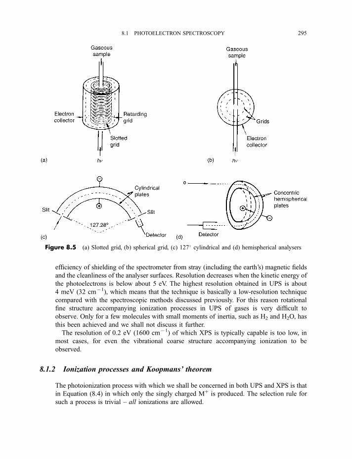
efficiency of shielding of the spectrometer from stray (including the earth’s) magnetic fields
and the cleanliness of the analyser surfaces. Resolution decreases when the kinetic energy of
the photoelectrons is below about 5 eV. The highest resolution obtained in UPS is about
4 meV (32 cm71), which means that the technique is basically a low-resolution technique
compared with the spectroscopic methods discussed previously. For this reason rotational
fine structure accompanying ionization processes in UPS of gases is very difficult to
observe. Only for a few molecules with small moments of inertia, such as H2 and H2O, has
this been achieved and we shall not discuss it further.
The resolution of 0.2 eV (1600 cm71) of which XPS is typically capable is too low, in
most cases, for even the vibrational coarse structure accompanying ionization to be
observed.
8.1.2 Ionization processes and Koopmans’ theorem
The photoionization process with which we shall be concerned in both UPS and XPS is that
in Equation (8.4) in which only the singly charged Mþ is produced. The selection rule for
such a process is trivial – all ionizations are allowed.
Figure 8.5 (a) Slotted grid, (b) spherical grid, (c) 127� cylindrical and (d) hemispherical analysers
8.1 PHOTOELECTRON SPECTROSCOPY 295
When M is an atom the total change in angular momentum for the process
Mþ hn! Mþ þ e must obey the electric dipole selection rule D‘ ¼ �1 (see Equation
7.21), but the photoelectron can take away any amount of momentum. If, for example, the
electron removed is from a d orbital ð‘ ¼ 2Þ of M it carries away one or three quanta of
angular momentum depending on whether D‘ ¼ �1 or þ1; respectively. The wave functionof a free electron can be described, in general, as a mixture of s, p, d, f , . . . wave functionsbut, in this case, the ejected electron has just p and f character.
In molecules, also, there is no restriction on the removal of an electron. The main
difference from atoms is that, since the symmetry is lower, the MOs themselves are mixtures
of s, p, d, f , . . . AOs and the ejected electron is described by a more complex mixture of s, p,
d, f , . . . character.From Figures 8.1(a) and 8.1(b) it would appear that the energy required to eject an
electron from an orbital (atomic or molecular) is a direct measure of the orbital energy. This
is approximately true and was originally proposed by Koopmans whose theorem can be
stated as follows: ‘For a closed-shell molecule the ionization energy of an electron in a
particular orbital is approximately equal to the negative of the orbital energy calculated by a
self-consistent field (SCF; see Section 7.1.1) method’, or, for orbital i,
Ii ’ �eSCFi ð8:5Þ
The negative sign is due to the convention that orbital energies ei are negative.
At the level of simple valence theory Koopmans’ theorem seems to be so self-evident as to
be scarcely worth stating. However, with more accurate theory, this is no longer so and great
interest attaches to why Equation (8.5) is only approximately true.
The measured ionization energy Ii is the difference in energy between M and Mþ, but theapproximation arises in equating this with the orbital energy. Orbitals are an entirely
theoretical concept and their energies can be obtained exactly only by calculation and then,
for a many-electron system, only with difficulty. Experimental ionization energies are the
measurable quantities that correspond most closely to the orbital energies.
The three most important factors that may contribute to the approximation in Equation
(8.5) relate to the main deficiencies in SCF calculations and are:
1. Electron reorganization. The orbitals in Mþ are not quite the same as in M because there
is one electron fewer. The electrons in Mþ are, therefore, in orbitals which are slightly
reorganized relative to those calculated for M, that is:
eSCFi ðMþÞ 6¼ eSCFi ðMÞ ð8:6Þ
2. Electron correlation. Electrons in an atom or molecule do not move entirely
independently of each other but their movements are correlated. The associated
correlation energy is often neglected in SCF calculations.
3. Relativistic effects. The neglect of the effects of relativity on orbital energies is another
common defect of SCF calculations and is particularly important for core orbital energies
which can be very large.
296 8 PHOTOELECTRON AND RELATED SPECTROSCOPIES
In most cases of closed-shell molecules Koopmans’ theorem is a reasonable approximation
but N2 (see Section 8.1.3.2b) is a notable exception. For open-shell molecules, such as O2
and NO, the theorem does not apply.
8.1.3 Photoelectron spectra and their interpretation
The simplest, and perhaps the most important, information derived from photoelectron
spectra is the ionization energies for valence and core electrons. Before the development of
photoelectron spectroscopy very few of these were known, especially for polyatomic
molecules. For core electrons ionization energies were previously unobtainable and illustrate
the extent to which core orbitals differ from the pure atomic orbitals pictured in simple
valence theory.
Because of the general validity of Koopmans’ theorem for closed-shell molecules
ionization energies and, as we shall see, the associated vibrational structure represent a vivid
illustration of the validity of quite simple-minded MO theory of valence electrons.
8.1.3.1 Ultraviolet photoelectron spectra of atoms
In the case of atoms UPS is unlikely to produce information which is not available from
other sources. In addition many materials have such low vapour pressures that their UPS
spectra may be recorded only at high temperatures. The noble gases, mercury and, to some
extent, the alkali metals are exceptions but we will consider here only the spectrum of argon.
The He I (21.22 eV) spectrum of argon is shown in Figure 8.6. The two peaks both result
from the removal of an electron from the 3p orbital in the process:
ArðKL3s23p6Þ ! ArþðKL3s23p5Þ ð8:7Þ
From the discussion in Section 7.1.2.3 we can deduce that the state arising from the ground
configuration of Ar is 1S0. However, the ground configuration of Arþ gives rise to two states,
2P1=2 and2P3=2, since L ¼ 1 and S ¼ 1
2, giving a 2P term, and J ¼ 1
2or 3
2. These two states of
Arþ are split by spin–orbit coupling. Since the unfilled 3p orbital is more than half-filled the
multiplet is inverted, the 2P3=2 state being below2P1=2 (Rule 4 on page 212). The splitting by
0.178 eV of the two peaks in Figure 8.6 reflects the spin–orbit coupling. The ionization
process Arþð2P3=2Þ � Arð1S0Þ is approximately twice as intense as Arþð2P1=2Þ � Arð1S0Þ.This is due to the four-fold degeneracy of the 2P3=2 state, resulting from MJ ¼ 3
2, 12, � 1
2, � 3
2,
compared with the two-fold degeneracy of the 2P1=2 state, for which MJ ¼ þ 12, � 1
2.
The He I ultraviolet photoelectron spectra of Kr and Xe appear similar to that of Ar but
the ionization energy decreases and the spin–orbit coupling increases with increasing atomic
number, as illustrated by the data in Table 8.1.
8.1 PHOTOELECTRON SPECTROSCOPY 297
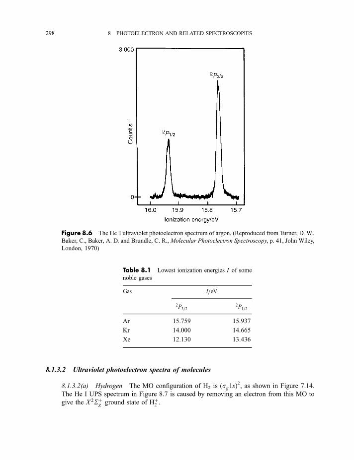
8.1.3.2 Ultraviolet photoelectron spectra of molecules
8.1.3.2(a) Hydrogen The MO configuration of H2 is ðsg1sÞ2, as shown in Figure 7.14.
The He I UPS spectrum in Figure 8.7 is caused by removing an electron from this MO to
give the X 2Sþg ground state of Hþ2 .
Figure 8.6 The He I ultraviolet photoelectron spectrum of argon. (Reproduced from Turner, D. W.,
Baker, C., Baker, A. D. and Brundle, C. R., Molecular Photoelectron Spectroscopy, p. 41, John Wiley,
London, 1970)
Table 8.1 Lowest ionization energies I of some
noble gases
Gas I=eV
2P3=22P1=2
Ar 15.759 15.937
Kr 14.000 14.665
Xe 12.130 13.436
298 8 PHOTOELECTRON AND RELATED SPECTROSCOPIES
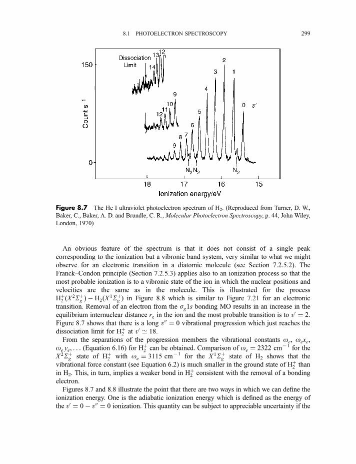
An obvious feature of the spectrum is that it does not consist of a single peak
corresponding to the ionization but a vibronic band system, very similar to what we might
observe for an electronic transition in a diatomic molecule (see Section 7.2.5.2). The
Franck–Condon principle (Section 7.2.5.3) applies also to an ionization process so that the
most probable ionization is to a vibronic state of the ion in which the nuclear positions and
velocities are the same as in the molecule. This is illustrated for the process
Hþ2 ðX 2Sþg Þ � H2ðX 1Sþg Þ in Figure 8.8 which is similar to Figure 7.21 for an electronic
transition. Removal of an electron from the sg1s bonding MO results in an increase in the
equilibrium internuclear distance re in the ion and the most probable transition is to v0 ¼ 2.
Figure 8.7 shows that there is a long v00 ¼ 0 vibrational progression which just reaches the
dissociation limit for Hþ2 at v0 ’ 18.
From the separations of the progression members the vibrational constants oe, oexe,
oe ye, . . . (Equation 6.16) for Hþ2 can be obtained. Comparison of oe ¼ 2322 cm71 for the
X 2Sþg state of Hþ2 with oe ¼ 3115 cm71 for the X 1Sþg state of H2 shows that the
vibrational force constant (see Equation 6.2) is much smaller in the ground state of Hþ2 than
in H2. This, in turn, implies a weaker bond in Hþ2 consistent with the removal of a bonding
electron.
Figures 8.7 and 8.8 illustrate the point that there are two ways in which we can define the
ionization energy. One is the adiabatic ionization energy which is defined as the energy of
the v0 ¼ 0� v00 ¼ 0 ionization. This quantity can be subject to appreciable uncertainty if the
Figure 8.7 The He I ultraviolet photoelectron spectrum of H2. (Reproduced from Turner, D. W.,
Baker, C., Baker, A. D. and Brundle, C. R., Molecular Photoelectron Spectroscopy, p. 44, John Wiley,
London, 1970)
8.1 PHOTOELECTRON SPECTROSCOPY 299
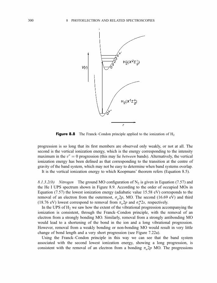
progression is so long that its first members are observed only weakly, or not at all. The
second is the vertical ionization energy, which is the energy corresponding to the intensity
maximum in the v00 ¼ 0 progression (this may lie between bands). Alternatively, the vertical
ionization energy has been defined as that corresponding to the transition at the centre of
gravity of the band system, which may not be easy to determine when band systems overlap.
It is the vertical ionization energy to which Koopmans’ theorem refers (Equation 8.5).
8.1.3.2(b) Nitrogen The ground MO configuration of N2 is given in Equation (7.57) and
the He I UPS spectrum shown in Figure 8.9. According to the order of occupied MOs in
Equation (7.57) the lowest ionization energy (adiabatic value 15.58 eV) corresponds to the
removal of an electron from the outermost, sg2p, MO. The second (16.69 eV) and third
(18.76 eV) lowest correspond to removal from pu2p and su*2s; respectively.In the UPS of H2 we saw how the extent of the vibrational progression accompanying the
ionization is consistent, through the Franck–Condon principle, with the removal of an
electron from a strongly bonding MO. Similarly, removal from a strongly antibonding MO
would lead to a shortening of the bond in the ion and a long vibrational progression.
However, removal from a weakly bonding or non-bonding MO would result in very little
change of bond length and a very short progression (see Figure 7.22a).
Using the Franck–Condon principle in this way we can see that the band system
associated with the second lowest ionization energy, showing a long progression, is
consistent with the removal of an electron from a bonding pu2p MO. The progressions
Figure 8.8 The Franck–Condon principle applied to the ionization of H2
300 8 PHOTOELECTRON AND RELATED SPECTROSCOPIES
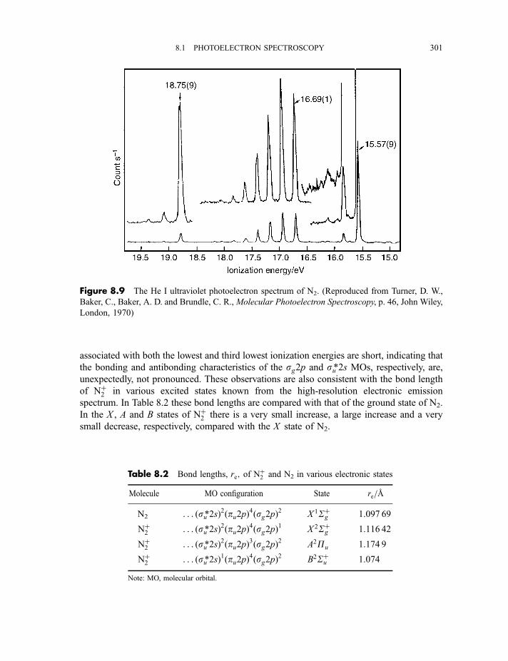
associated with both the lowest and third lowest ionization energies are short, indicating that
the bonding and antibonding characteristics of the sg2p and su*2s MOs, respectively, are,
unexpectedly, not pronounced. These observations are also consistent with the bond length
of Nþ2 in various excited states known from the high-resolution electronic emission
spectrum. In Table 8.2 these bond lengths are compared with that of the ground state of N2.
In the X , A and B states of Nþ2 there is a very small increase, a large increase and a very
small decrease, respectively, compared with the X state of N2.
Figure 8.9 The He I ultraviolet photoelectron spectrum of N2. (Reproduced from Turner, D. W.,
Baker, C., Baker, A. D. and Brundle, C. R., Molecular Photoelectron Spectroscopy, p. 46, John Wiley,
London, 1970)
Table 8.2 Bond lengths, re; of Nþ2 and N2 in various electronic states
Molecule MO configuration State re=A
N2 . . . ðsu*2sÞ2ðpu2pÞ4ðsg2pÞ2 X 1Sþg 1.097 69
Nþ2 . . . ðsu*2sÞ2ðpu2pÞ4ðsg2pÞ1 X 2Sþg 1.116 42
Nþ2 . . . ðsu*2sÞ2ðpu2pÞ3ðsg2pÞ2 A2Pu 1.174 9
Nþ2 . . . ðsu*2sÞ1ðpu2pÞ4ðsg2pÞ2 B2Sþu 1.074
Note: MO, molecular orbital.
8.1 PHOTOELECTRON SPECTROSCOPY 301
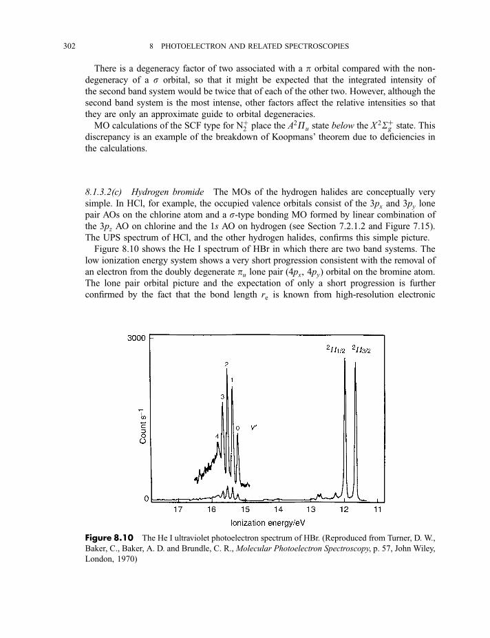
There is a degeneracy factor of two associated with a p orbital compared with the non-
degeneracy of a s orbital, so that it might be expected that the integrated intensity of
the second band system would be twice that of each of the other two. However, although the
second band system is the most intense, other factors affect the relative intensities so that
they are only an approximate guide to orbital degeneracies.
MO calculations of the SCF type for Nþ2 place the A2Pu state below the X 2Sþg state. This
discrepancy is an example of the breakdown of Koopmans’ theorem due to deficiencies in
the calculations.
8.1.3.2(c) Hydrogen bromide The MOs of the hydrogen halides are conceptually very
simple. In HCl, for example, the occupied valence orbitals consist of the 3px and 3py lone
pair AOs on the chlorine atom and a s-type bonding MO formed by linear combination of
the 3pz AO on chlorine and the 1s AO on hydrogen (see Section 7.2.1.2 and Figure 7.15).
The UPS spectrum of HCl, and the other hydrogen halides, confirms this simple picture.
Figure 8.10 shows the He I spectrum of HBr in which there are two band systems. The
low ionization energy system shows a very short progression consistent with the removal of
an electron from the doubly degenerate pu lone pair (4px, 4py) orbital on the bromine atom.
The lone pair orbital picture and the expectation of only a short progression is further
confirmed by the fact that the bond length re is known from high-resolution electronic
Figure 8.10 The He I ultraviolet photoelectron spectrum of HBr. (Reproduced from Turner, D. W.,
Baker, C., Baker, A. D. and Brundle, C. R., Molecular Photoelectron Spectroscopy, p. 57, John Wiley,
London, 1970)
302 8 PHOTOELECTRON AND RELATED SPECTROSCOPIES
spectroscopy to be 1.4144 A in the X 1Sþ ground state of HBr and to have a fairly similar
value of 1.4484 A in the X 2P ground state of HBrþ
The splitting by 0.33 eVof the X 2P state into an inverted multiplet, with the 2P3=2 below
the 2P1=2 component, is relatively large due to the spin–orbit coupling caused by the high
nuclear charge on the bromine atom and also the fact that the orbital from which the electron
has been removed is close to this atom. The corresponding splittings in the X 2P states of
HCl and HI are 0.08 and 0.66 eV, respectively, consistent with the magnitude of the nuclear
charge on Cl and I.
Figure 8.10 shows that the next band system of HBr consists of a fairly long progression
with a maximum intensity at v0 ¼ 2. A long progression is to be expected following the
removal of an electron from the strongly bonding s MO to form the A2Sþ state of HBrþ, inwhich re has the value of 1.6842 A, an increase of about 0.27 A from that of HBr. There is
no spin–orbit interaction in 2Sþ states since they have no orbital angular momentum (see
Section 7.2.2). Consequently, there is no doubling of bands in this system of the ultraviolet
photoelectron spectrum.
Worked example 8.1
Question. Which low-lying states of NOþ would you expect to feature in the He I ultraviolet
photoelectron spectrum of NO? (Consider removal of an electron from only the three outermost
orbitals of NO.) Indicate whether a long or short vibrational progression would be anticipated in
each case.
Answer. The ground molecular orbital configuration of the electrons in NO is (see also
Section 7.2.1.2)
ðs1sÞ2ðs*1sÞ2ðs2sÞ2ðs*2sÞ2ðs2pÞ2ðp2pÞ4ðp*2pÞ1
To derive the states arising from a molecular orbital configuration in a diatomic molecule see
Sections 7.2.2 and 7.2.4. There are two states, 2P1=2 and2P3=2, arising from this configuration
and 2P1=2 is the lower in energy and, therefore, the ground state.
Removal of an electron from the outermost, p*2p, orbital results in the configuration
NOþ . . . ðs2pÞ2ðp2pÞ4ðp*2pÞ0
which gives rise to just one state, 1Sþ, the ground state of NOþ. Since the orbital from which
the electron has been removed is antibonding, we would expect a shortening of the bond and a
reasonably long vibrational progression. The He I photoelectron spectrum below shows that this
is the case. The ionisation energy is 9.26 eV.
Removal of an electron from the p2p orbital gives the configuration
NOþ . . . ðs2pÞ2ðp2pÞ3ðp*2pÞ1
8.1 PHOTOELECTRON SPECTROSCOPY 303
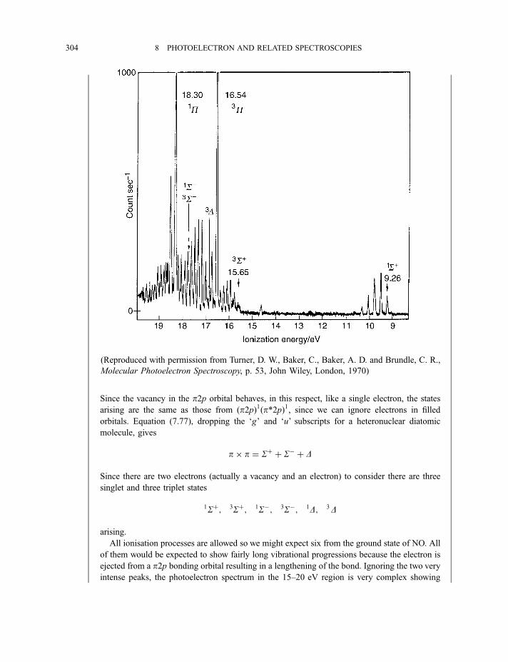
Since the vacancy in the p2p orbital behaves, in this respect, like a single electron, the states
arising are the same as those from ðp2pÞ1ðp*2pÞ1, since we can ignore electrons in filled
orbitals. Equation (7.77), dropping the ‘g’ and ‘u’ subscripts for a heteronuclear diatomic
molecule, gives
p� p ¼ Sþ þ S� þ D
Since there are two electrons (actually a vacancy and an electron) to consider there are three
singlet and three triplet states
1Sþ; 3Sþ; 1S�; 3S�; 1D; 3D
arising.
All ionisation processes are allowed so we might expect six from the ground state of NO. All
of them would be expected to show fairly long vibrational progressions because the electron is
ejected from a p2p bonding orbital resulting in a lengthening of the bond. Ignoring the two veryintense peaks, the photoelectron spectrum in the 15–20 eV region is very complex showing
(Reproduced with permission from Turner, D. W., Baker, C., Baker, A. D. and Brundle, C. R.,
Molecular Photoelectron Spectroscopy, p. 53, John Wiley, London, 1970)
304 8 PHOTOELECTRON AND RELATED SPECTROSCOPIES
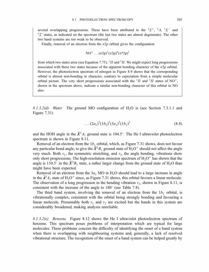
several overlapping progressions. These have been attributed to the 3Sþ, 3D, 1S� and3S�states, as indicated on the spectrum (the last two states are almost degenerate). The other
two band systems are too weak to be observed.
Finally, removal of an electron from the s2p orbital gives the configuration
NOþ . . . ðs2pÞ1ðp2pÞ4ðp*2pÞ1
from which two states arise (see Equation 7.75), 1P and 3P. We might expect long progressions
associated with these two states because of the apparent bonding character of the s2p orbital.
However, the photoelectron spectrum of nitrogen in Figure 8.9 shows that the corresponding
orbital is almost non-bonding in character, contrary to expectation from a simple molecular
orbital picture. The very short progressions associated with the 1P and 3P states of NOþ,shown in the spectrum above, indicate a similar non-bonding character of this orbital in NO
also.
8.1.3.2(d) Water The ground MO configuration of H2O is (see Section 7.3.1.1 and
Figure 7.31)
. . . ð2a1Þ2ð1b2Þ2ð3a1Þ2ð1b1Þ2 ð8:8Þ
and the HOH angle in the ~XX 1A1 ground state is 104.5�. The He I ultraviolet photoelectron
spectrum is shown in Figure 8.11.
Removal of an electron from the 1b1 orbital, which, as Figure 7.31 shows, does not favour
any particular bond angle, to give the ~XX 2B1 ground state of H2Oþ should not affect the angle
very much. Both n1, the symmetric stretching, and n2, the angle bending, vibrations show
only short progressions. The high-resolution emission spectrum of H2Oþ has shown that the
angle is 110.5� in the ~XX 2B1 state, a rather larger change from the ground state of H2O than
might have been expected.
Removal of an electron from the 3a1 MO in H2O should lead to a large increase in angle
in the ~AA2A1 state of H2Oþ since, as Figure 7.31 shows, this orbital favours a linear molecule.
The observation of a long progression in the bending vibration n2, shown in Figure 8.11, is
consistent with the increase of the angle to 180� (see Table 7.8).
The third band system, involving the removal of an electron from the 1b2 orbital, is
vibrationally complex, consistent with the orbital being strongly bonding and favouring a
linear molecule. Presumably both n1 and n2 are excited but the bands in this system are
considerably broadened, making analysis unreliable.
8.1.3.2(e) Benzene Figure 8.12 shows the He I ultraviolet photoelectron spectrum of
benzene. This spectrum poses problems of interpretation which are typical for large
molecules. These problems concern the difficulty of identifying the onset of a band system
when there is overlapping with neighbouring systems and, generally, a lack of resolved
vibrational structure. The recognition of the onset of a band system can be helped greatly by
8.1 PHOTOELECTRON SPECTROSCOPY 305
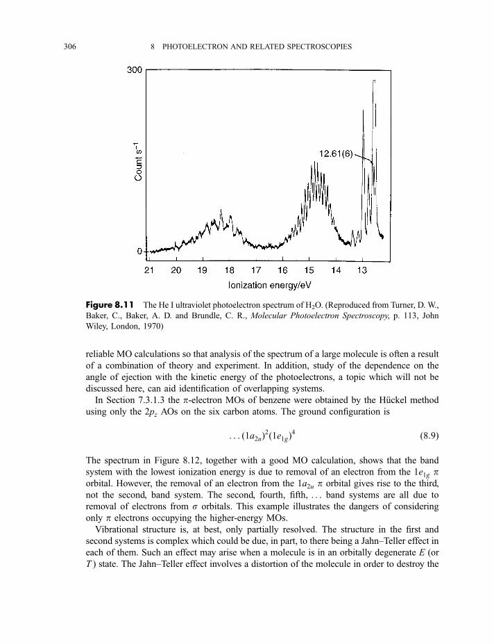
reliable MO calculations so that analysis of the spectrum of a large molecule is often a result
of a combination of theory and experiment. In addition, study of the dependence on the
angle of ejection with the kinetic energy of the photoelectrons, a topic which will not be
discussed here, can aid identification of overlapping systems.
In Section 7.3.1.3 the p-electron MOs of benzene were obtained by the Huckel method
using only the 2pz AOs on the six carbon atoms. The ground configuration is
. . . ð1a2uÞ2ð1e1gÞ4 ð8:9Þ
The spectrum in Figure 8.12, together with a good MO calculation, shows that the band
system with the lowest ionization energy is due to removal of an electron from the 1e1g porbital. However, the removal of an electron from the 1a2u p orbital gives rise to the third,
not the second, band system. The second, fourth, fifth, . . . band systems are all due to
removal of electrons from s orbitals. This example illustrates the dangers of considering
only p electrons occupying the higher-energy MOs.
Vibrational structure is, at best, only partially resolved. The structure in the first and
second systems is complex which could be due, in part, to there being a Jahn–Teller effect in
each of them. Such an effect may arise when a molecule is in an orbitally degenerate E (or
T ) state. The Jahn–Teller effect involves a distortion of the molecule in order to destroy the
Figure 8.11 The He I ultraviolet photoelectron spectrum of H2O. (Reproduced from Turner, D. W.,
Baker, C., Baker, A. D. and Brundle, C. R., Molecular Photoelectron Spectroscopy, p. 113, John
Wiley, London, 1970)
306 8 PHOTOELECTRON AND RELATED SPECTROSCOPIES
degeneracy. The only relatively simple structure is observed in the seventh system in which
an electron is removed from the 3a1g orbital. There is a long progression in n1, the a1g ring-breathing vibration (see Figure 6.13f ) consistent with the electron coming from a s CC
bonding orbital.
8.1.3.3 X-ray photoelectron spectra of gases
We have seen above how X-ray photons may eject an electron from the core orbitals of an
atom, whether it is free or part of a molecule. So far, in all aspects of valence theory of
molecules that we have considered, the core electrons have been assumed to be in orbitals
which are unchanged from the AOs of the corresponding atoms. XPS demonstrates that this
is almost, but not quite, true.
This point is illustrated in Figure 8.13 which shows the X-ray photoelectron spectrum of a
2 : 1 mixture of CO and CO2 gases obtained with MgKa (1253.7 eV) source radiation. The
ionization energy for removal of an electron from the 1s orbital on a carbon atom, referred to
as the C 1s ionization energy, is 295.8 eV in CO and 297.8 eV in CO2, these being quite
comfortably resolved. The O 1s ionization energy is 541.1 eV in CO and 539.8 eV in CO2,
which are also resolved.
There are two features which stand out from these data. The first is that the ionization
energy is much greater for O 1s than for C 1s due to the effect of the larger nuclear charge on
oxygen. The second effect is that the ionization energy for a particular core orbital in a
particular atom depends on the immediate environment in the molecule. This latter effect is
known as the chemical shift. It is not to be confused with the chemical shift in nuclear
magnetic resonance (NMR) spectroscopy which is the shift of the signal due to the nuclear
Figure 8.12 The He I ultraviolet photoelectron spectrum of benzene. (Reproduced from Karlsson,
L., Mattsson, L., Jadrny, R., Bergmark, T. and Siegbahn, K., Physica Scripta, 14, 230, 1976)
8.1 PHOTOELECTRON SPECTROSCOPY 307
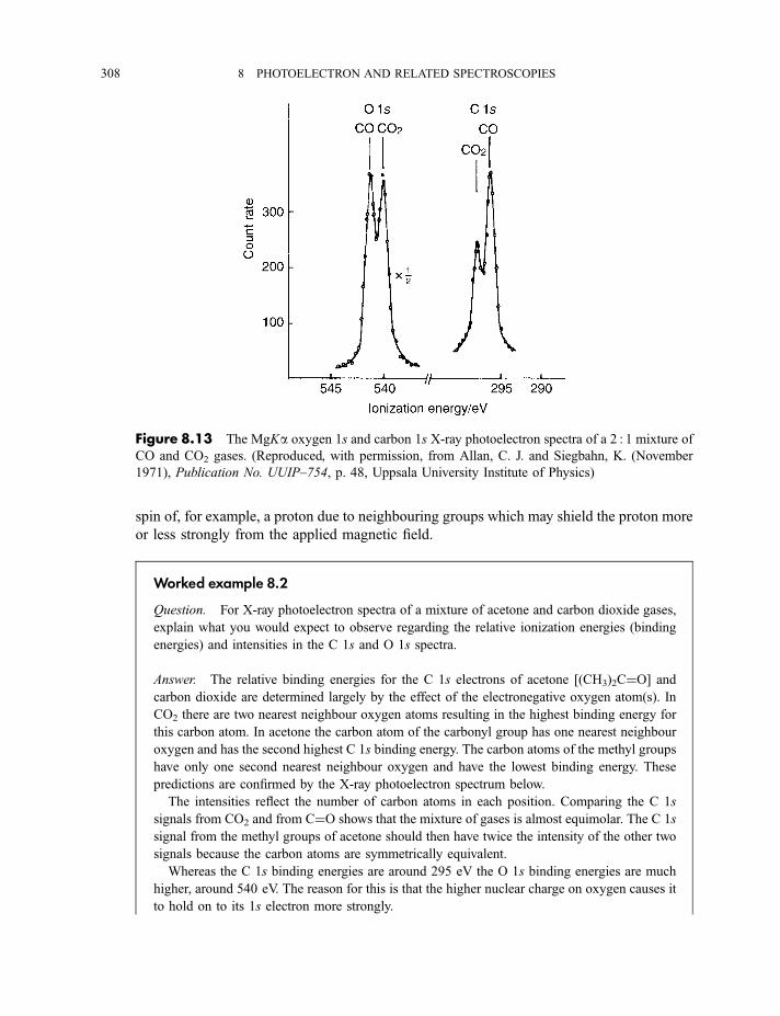
spin of, for example, a proton due to neighbouring groups which may shield the proton more
or less strongly from the applied magnetic field.
Worked example 8.2
Question. For X-ray photoelectron spectra of a mixture of acetone and carbon dioxide gases,
explain what you would expect to observe regarding the relative ionization energies (binding
energies) and intensities in the C 1s and O 1s spectra.
Answer. The relative binding energies for the C 1s electrons of acetone [(CH3)2C¼O] andcarbon dioxide are determined largely by the effect of the electronegative oxygen atom(s). In
CO2 there are two nearest neighbour oxygen atoms resulting in the highest binding energy for
this carbon atom. In acetone the carbon atom of the carbonyl group has one nearest neighbour
oxygen and has the second highest C 1s binding energy. The carbon atoms of the methyl groups
have only one second nearest neighbour oxygen and have the lowest binding energy. These
predictions are confirmed by the X-ray photoelectron spectrum below.
The intensities reflect the number of carbon atoms in each position. Comparing the C 1s
signals from CO2 and from C¼O shows that the mixture of gases is almost equimolar. The C 1s
signal from the methyl groups of acetone should then have twice the intensity of the other two
signals because the carbon atoms are symmetrically equivalent.
Whereas the C 1s binding energies are around 295 eV the O 1s binding energies are much
higher, around 540 eV. The reason for this is that the higher nuclear charge on oxygen causes it
to hold on to its 1s electron more strongly.
Figure 8.13 The MgKa oxygen 1s and carbon 1s X-ray photoelectron spectra of a 2 : 1 mixture of
CO and CO2 gases. (Reproduced, with permission, from Allan, C. J. and Siegbahn, K. (November
1971), Publication No. UUIP–754, p. 48, Uppsala University Institute of Physics)
308 8 PHOTOELECTRON AND RELATED SPECTROSCOPIES
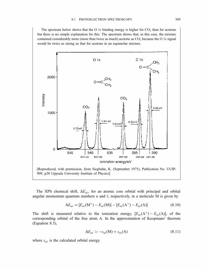
The spectrum below shows that the O 1s binding energy is higher for CO2 than for acetone
but there is no simple explanation for this. The spectrum shows that, in this case, the mixture
contained considerably more (more than twice as much) acetone as CO2 because the O 1s signal
would be twice as strong as that for acetone in an equimolar mixture.
The XPS chemical shift, DEn‘, for an atomic core orbital with principal and orbital
angular momentum quantum numbers n and ‘, respectively, in a molecule M is given by
DEn‘ ¼ ½En‘ðMþÞ � En‘ðMÞ� � ½En‘ðAþÞ � En‘ðAÞ� ð8:10Þ
The shift is measured relative to the ionization energy, ½En‘ðAþÞ � En‘ðAÞ�, of the
corresponding orbital of the free atom A. In the approximation of Koopmans’ theorem
(Equation 8.5),
DEn‘ ’ �en‘ðMÞ þ en‘ðAÞ ð8:11Þ
where en‘ is the calculated orbital energy.
[Reproduced, with permission, from Siegbahn, K. (September 1975), Publication No. UUIP-
909, p20 Uppsala University Institute of Physics]
8.1 PHOTOELECTRON SPECTROSCOPY 309
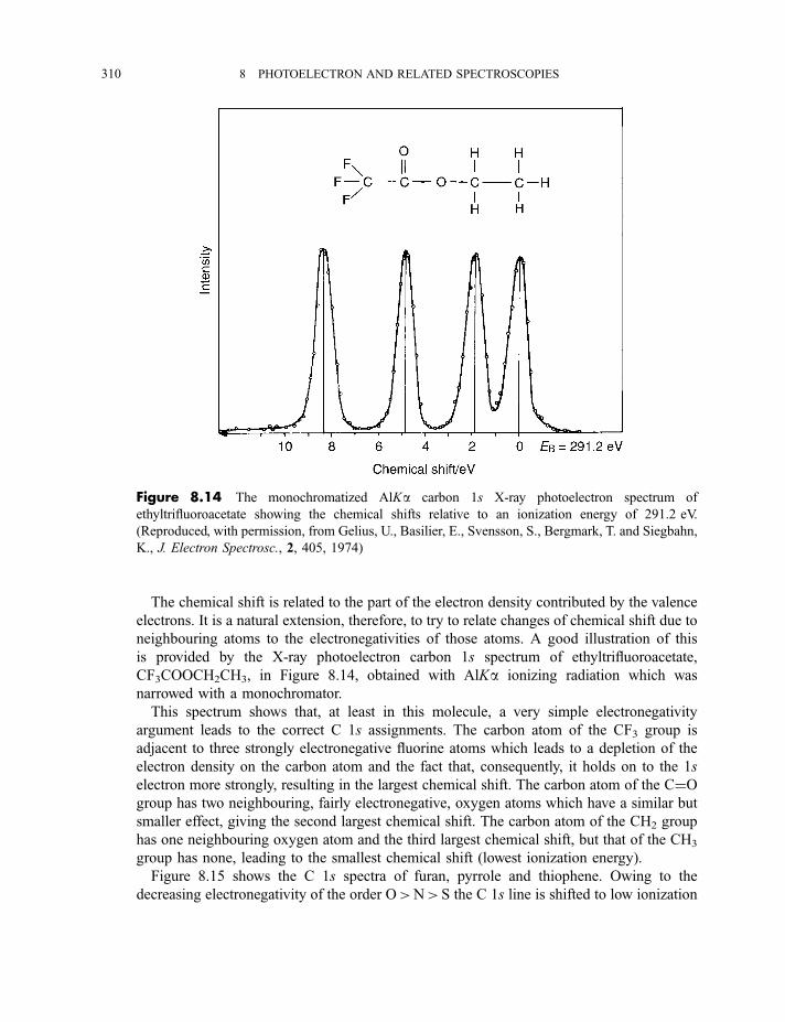
The chemical shift is related to the part of the electron density contributed by the valence
electrons. It is a natural extension, therefore, to try to relate changes of chemical shift due to
neighbouring atoms to the electronegativities of those atoms. A good illustration of this
is provided by the X-ray photoelectron carbon 1s spectrum of ethyltrifluoroacetate,
CF3COOCH2CH3, in Figure 8.14, obtained with AlKa ionizing radiation which was
narrowed with a monochromator.
This spectrum shows that, at least in this molecule, a very simple electronegativity
argument leads to the correct C 1s assignments. The carbon atom of the CF3 group is
adjacent to three strongly electronegative fluorine atoms which leads to a depletion of the
electron density on the carbon atom and the fact that, consequently, it holds on to the 1s
electron more strongly, resulting in the largest chemical shift. The carbon atom of the C¼Ogroup has two neighbouring, fairly electronegative, oxygen atoms which have a similar but
smaller effect, giving the second largest chemical shift. The carbon atom of the CH2 group
has one neighbouring oxygen atom and the third largest chemical shift, but that of the CH3
group has none, leading to the smallest chemical shift (lowest ionization energy).
Figure 8.15 shows the C 1s spectra of furan, pyrrole and thiophene. Owing to the
decreasing electronegativity of the order O>N>S the C 1s line is shifted to low ionization
Figure 8.14 The monochromatized AlKa carbon 1s X-ray photoelectron spectrum of
ethyltrifluoroacetate showing the chemical shifts relative to an ionization energy of 291.2 eV.
(Reproduced, with permission, from Gelius, U., Basilier, E., Svensson, S., Bergmark, T. and Siegbahn,
K., J. Electron Spectrosc., 2, 405, 1974)
310 8 PHOTOELECTRON AND RELATED SPECTROSCOPIES
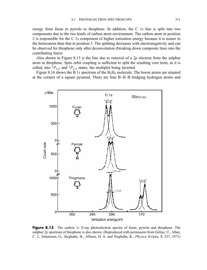
energy from furan to pyrrole to thiophene. In addition, the C 1s line is split into two
components due to the two kinds of carbon atom environment. The carbon atom in position
2 is responsible for the C 1s component of higher ionization energy because it is nearer to
the heteroatom than that in position 3. The splitting decreases with electronegativity and can
be observed for thiophene only after deconvolution (breaking down composite lines into the
contributing lines).
Also shown in Figure 8.15 is the line due to removal of a 2p electron from the sulphur
atom in thiophene. Spin–orbit coupling is sufficient to split the resulting core term, as it is
called, into 2P3=2 and 2P1=2 states, the multiplet being inverted.
Figure 8.16 shows the B 1s spectrum of the B5H9 molecule. The boron atoms are situated
at the corners of a square pyramid. There are four B–H–B bridging hydrogen atoms and
Figure 8.15 The carbon 1s X-ray photoelectron spectra of furan, pyrrole and thiophene. The
sulphur 2p spectrum of thiophene is also shown. (Reproduced with permission from Gelius, U., Allan,
C. J., Johansson, G., Siegbahn, H., Allison, D. A. and Siegbahn, K., Physica Scripta, 3, 237, 1971)
8.1 PHOTOELECTRON SPECTROSCOPY 311
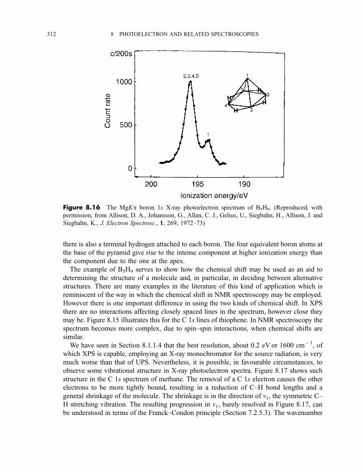
there is also a terminal hydrogen attached to each boron. The four equivalent boron atoms at
the base of the pyramid give rise to the intense component at higher ionization energy than
the component due to the one at the apex.
The example of B5H9 serves to show how the chemical shift may be used as an aid to
determining the structure of a molecule and, in particular, in deciding between alternative
structures. There are many examples in the literature of this kind of application which is
reminiscent of the way in which the chemical shift in NMR spectroscopy may be employed.
However there is one important difference in using the two kinds of chemical shift. In XPS
there are no interactions affecting closely spaced lines in the spectrum, however close they
may be. Figure 8.15 illustrates this for the C 1s lines of thiophene. In NMR spectroscopy the
spectrum becomes more complex, due to spin–spin interactions, when chemical shifts are
similar.
We have seen in Section 8.1.1.4 that the best resolution, about 0.2 eV or 1600 cm71, of
which XPS is capable, employing an X-ray monochromator for the source radiation, is very
much worse than that of UPS. Nevertheless, it is possible, in favourable circumstances, to
observe some vibrational structure in X-ray photoelectron spectra. Figure 8.17 shows such
structure in the C 1s spectrum of methane. The removal of a C 1s electron causes the other
electrons to be more tightly bound, resulting in a reduction of C–H bond lengths and a
general shrinkage of the molecule. The shrinkage is in the direction of n1, the symmetric C–
H stretching vibration. The resulting progression in n1, barely resolved in Figure 8.17, can
be understood in terms of the Franck–Condon principle (Section 7.2.5.3). The wavenumber
Figure 8.16 The MgKa boron 1s X-ray photoelectron spectrum of B5H9. (Reproduced, with
permission, from Allison, D. A., Johansson, G., Allan, C. J., Gelius, U., Siegbahn, H., Allison, J. and
Siegbahn, K., J. Electron Spectrosc., 1, 269, 1972–73)
312 8 PHOTOELECTRON AND RELATED SPECTROSCOPIES
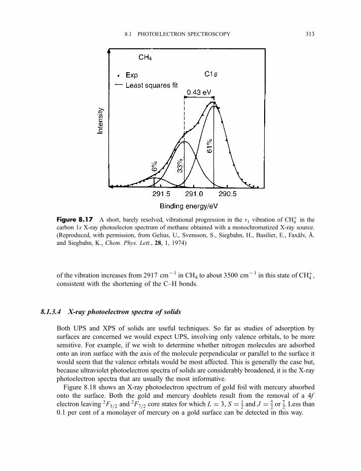
of the vibration increases from 2917 cm71 in CH4 to about 3500 cm71 in this state of CHþ4 ,consistent with the shortening of the C–H bonds.
8.1.3.4 X-ray photoelectron spectra of solids
Both UPS and XPS of solids are useful techniques. So far as studies of adsorption by
surfaces are concerned we would expect UPS, involving only valence orbitals, to be more
sensitive. For example, if we wish to determine whether nitrogen molecules are adsorbed
onto an iron surface with the axis of the molecule perpendicular or parallel to the surface it
would seem that the valence orbitals would be most affected. This is generally the case but,
because ultraviolet photoelectron spectra of solids are considerably broadened, it is the X-ray
photoelectron spectra that are usually the most informative.
Figure 8.18 shows an X-ray photoelectron spectrum of gold foil with mercury absorbed
onto the surface. Both the gold and mercury doublets result from the removal of a 4f
electron leaving 2F5=2 and2F7=2 core states for which L ¼ 3, S ¼ 1
2and J ¼ 5
2or 7
2. Less than
0.1 per cent of a monolayer of mercury on a gold surface can be detected in this way.
Figure 8.17 A short, barely resolved, vibrational progression in the n1 vibration of CHþ4 in the
carbon 1s X-ray photoelecton spectrum of methane obtained with a monochromatized X-ray source.
(Reproduced, with permission, from Gelius, U., Svensson, S., Siegbahn, H., Basilier, E., Faxalv, A.
and Siegbahn, K., Chem. Phys. Lett., 28, 1, 1974)
8.1 PHOTOELECTRON SPECTROSCOPY 313
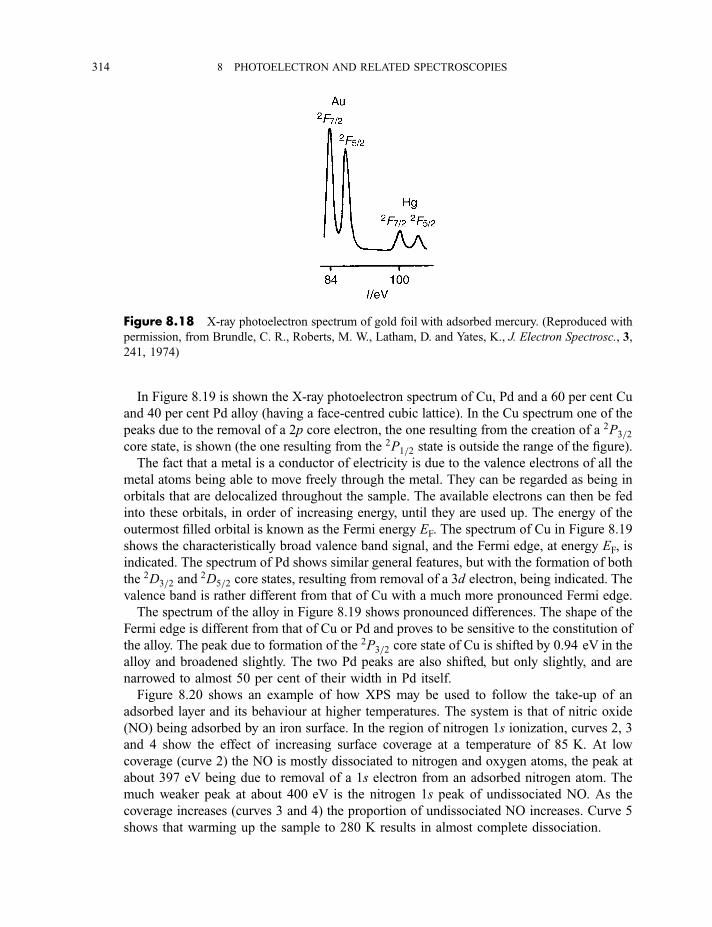
In Figure 8.19 is shown the X-ray photoelectron spectrum of Cu, Pd and a 60 per cent Cu
and 40 per cent Pd alloy (having a face-centred cubic lattice). In the Cu spectrum one of the
peaks due to the removal of a 2p core electron, the one resulting from the creation of a 2P3=2
core state, is shown (the one resulting from the 2P1=2 state is outside the range of the figure).
The fact that a metal is a conductor of electricity is due to the valence electrons of all the
metal atoms being able to move freely through the metal. They can be regarded as being in
orbitals that are delocalized throughout the sample. The available electrons can then be fed
into these orbitals, in order of increasing energy, until they are used up. The energy of the
outermost filled orbital is known as the Fermi energy EF. The spectrum of Cu in Figure 8.19
shows the characteristically broad valence band signal, and the Fermi edge, at energy EF, is
indicated. The spectrum of Pd shows similar general features, but with the formation of both
the 2D3=2 and2D5=2 core states, resulting from removal of a 3d electron, being indicated. The
valence band is rather different from that of Cu with a much more pronounced Fermi edge.
The spectrum of the alloy in Figure 8.19 shows pronounced differences. The shape of the
Fermi edge is different from that of Cu or Pd and proves to be sensitive to the constitution of
the alloy. The peak due to formation of the 2P3=2 core state of Cu is shifted by 0.94 eV in the
alloy and broadened slightly. The two Pd peaks are also shifted, but only slightly, and are
narrowed to almost 50 per cent of their width in Pd itself.
Figure 8.20 shows an example of how XPS may be used to follow the take-up of an
adsorbed layer and its behaviour at higher temperatures. The system is that of nitric oxide
(NO) being adsorbed by an iron surface. In the region of nitrogen 1s ionization, curves 2, 3
and 4 show the effect of increasing surface coverage at a temperature of 85 K. At low
coverage (curve 2) the NO is mostly dissociated to nitrogen and oxygen atoms, the peak at
about 397 eV being due to removal of a 1s electron from an adsorbed nitrogen atom. The
much weaker peak at about 400 eV is the nitrogen 1s peak of undissociated NO. As the
coverage increases (curves 3 and 4) the proportion of undissociated NO increases. Curve 5
shows that warming up the sample to 280 K results in almost complete dissociation.
Figure 8.18 X-ray photoelectron spectrum of gold foil with adsorbed mercury. (Reproduced with
permission, from Brundle, C. R., Roberts, M. W., Latham, D. and Yates, K., J. Electron Spectrosc., 3,
241, 1974)
314 8 PHOTOELECTRON AND RELATED SPECTROSCOPIES
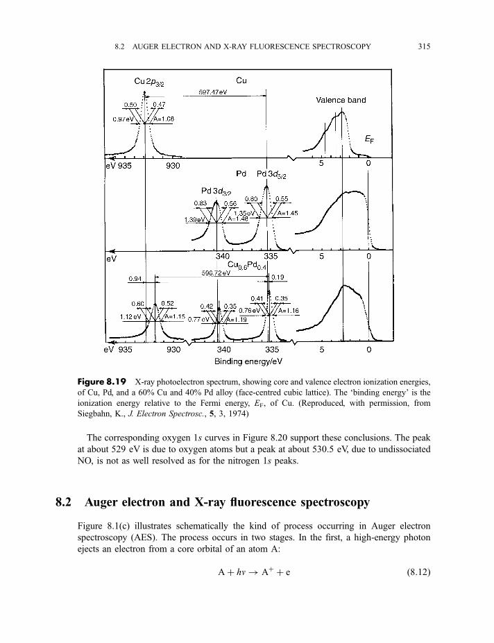
The corresponding oxygen 1s curves in Figure 8.20 support these conclusions. The peak
at about 529 eV is due to oxygen atoms but a peak at about 530.5 eV, due to undissociated
NO, is not as well resolved as for the nitrogen 1s peaks.
8.2 Auger electron and X-ray fluorescence spectroscopy
Figure 8.1(c) illustrates schematically the kind of process occurring in Auger electron
spectroscopy (AES). The process occurs in two stages. In the first, a high-energy photon
ejects an electron from a core orbital of an atom A:
Aþ hn! Aþ þ e ð8:12Þ
Figure 8.19 X-ray photoelectron spectrum, showing core and valence electron ionization energies,
of Cu, Pd, and a 60% Cu and 40% Pd alloy (face-centred cubic lattice). The ‘binding energy’ is the
ionization energy relative to the Fermi energy, EF, of Cu. (Reproduced, with permission, from
Siegbahn, K., J. Electron Spectrosc., 5, 3, 1974)
8.2 AUGER ELECTRON AND X-RAY FLUORESCENCE SPECTROSCOPY 315
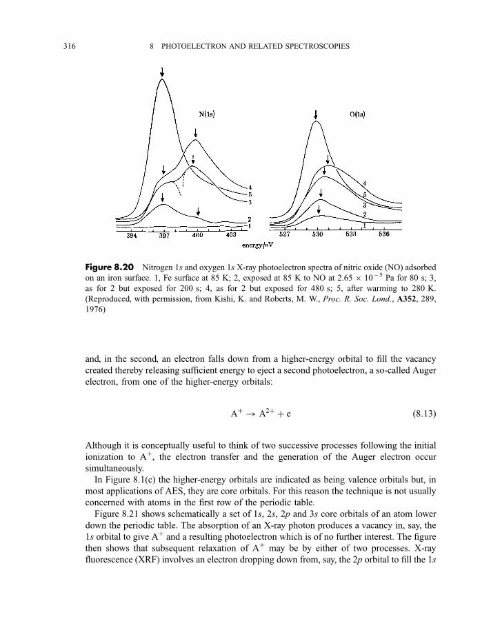
and, in the second, an electron falls down from a higher-energy orbital to fill the vacancy
created thereby releasing sufficient energy to eject a second photoelectron, a so-called Auger
electron, from one of the higher-energy orbitals:
Aþ ! A2þ þ e ð8:13Þ
Although it is conceptually useful to think of two successive processes following the initial
ionization to Aþ, the electron transfer and the generation of the Auger electron occur
simultaneously.
In Figure 8.1(c) the higher-energy orbitals are indicated as being valence orbitals but, in
most applications of AES, they are core orbitals. For this reason the technique is not usually
concerned with atoms in the first row of the periodic table.
Figure 8.21 shows schematically a set of 1s, 2s, 2p and 3s core orbitals of an atom lower
down the periodic table. The absorption of an X-ray photon produces a vacancy in, say, the
1s orbital to give Aþ and a resulting photoelectron which is of no further interest. The figure
then shows that subsequent relaxation of Aþ may be by either of two processes. X-ray
fluorescence (XRF) involves an electron dropping down from, say, the 2p orbital to fill the 1s
Figure 8.20 Nitrogen 1s and oxygen 1s X-ray photoelectron spectra of nitric oxide (NO) adsorbed
on an iron surface. 1, Fe surface at 85 K; 2, exposed at 85 K to NO at 2.656 1075 Pa for 80 s; 3,
as for 2 but exposed for 200 s; 4, as for 2 but exposed for 480 s; 5, after warming to 280 K.
(Reproduced, with permission, from Kishi, K. and Roberts, M. W., Proc. R. Soc. Lond., A352, 289,
1976)
316 8 PHOTOELECTRON AND RELATED SPECTROSCOPIES
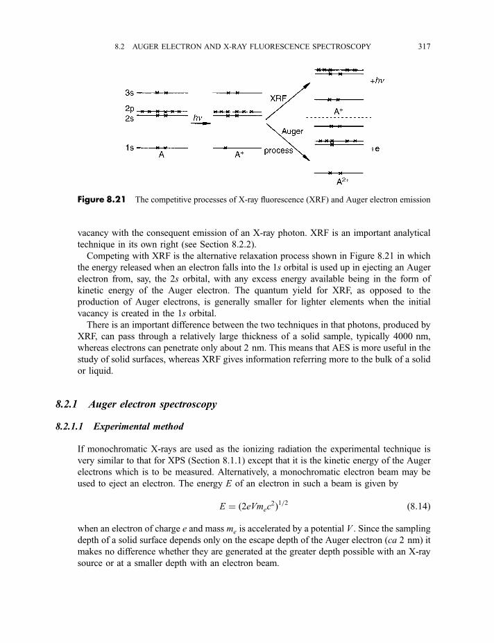
vacancy with the consequent emission of an X-ray photon. XRF is an important analytical
technique in its own right (see Section 8.2.2).
Competing with XRF is the alternative relaxation process shown in Figure 8.21 in which
the energy released when an electron falls into the 1s orbital is used up in ejecting an Auger
electron from, say, the 2s orbital, with any excess energy available being in the form of
kinetic energy of the Auger electron. The quantum yield for XRF, as opposed to the
production of Auger electrons, is generally smaller for lighter elements when the initial
vacancy is created in the 1s orbital.
There is an important difference between the two techniques in that photons, produced by
XRF, can pass through a relatively large thickness of a solid sample, typically 4000 nm,
whereas electrons can penetrate only about 2 nm. This means that AES is more useful in the
study of solid surfaces, whereas XRF gives information referring more to the bulk of a solid
or liquid.
8.2.1 Auger electron spectroscopy
8.2.1.1 Experimental method
If monochromatic X-rays are used as the ionizing radiation the experimental technique is
very similar to that for XPS (Section 8.1.1) except that it is the kinetic energy of the Auger
electrons which is to be measured. Alternatively, a monochromatic electron beam may be
used to eject an electron. The energy E of an electron in such a beam is given by
E ¼ ð2eVmec2Þ1=2 ð8:14Þ
when an electron of charge e and mass me is accelerated by a potential V . Since the sampling
depth of a solid surface depends only on the escape depth of the Auger electron (ca 2 nm) it
makes no difference whether they are generated at the greater depth possible with an X-ray
source or at a smaller depth with an electron beam.
Figure 8.21 The competitive processes of X-ray fluorescence (XRF) and Auger electron emission
8.2 AUGER ELECTRON AND X-RAY FLUORESCENCE SPECTROSCOPY 317
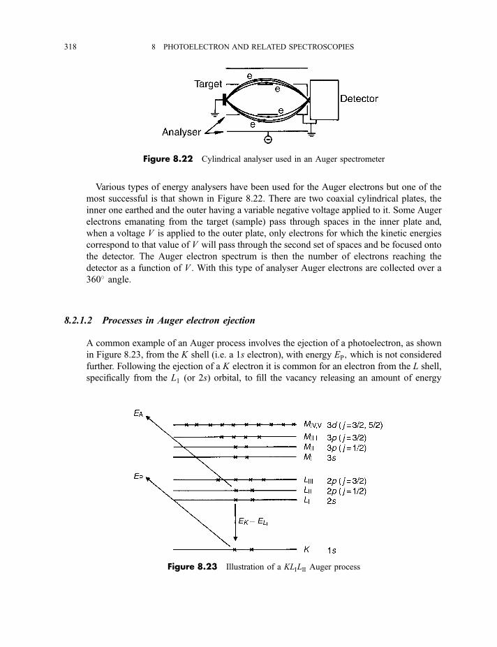
Various types of energy analysers have been used for the Auger electrons but one of the
most successful is that shown in Figure 8.22. There are two coaxial cylindrical plates, the
inner one earthed and the outer having a variable negative voltage applied to it. Some Auger
electrons emanating from the target (sample) pass through spaces in the inner plate and,
when a voltage V is applied to the outer plate, only electrons for which the kinetic energies
correspond to that value of V will pass through the second set of spaces and be focused onto
the detector. The Auger electron spectrum is then the number of electrons reaching the
detector as a function of V . With this type of analyser Auger electrons are collected over a
360� angle.
8.2.1.2 Processes in Auger electron ejection
A common example of an Auger process involves the ejection of a photoelectron, as shown
in Figure 8.23, from the K shell (i.e. a 1s electron), with energy EP; which is not considered
further. Following the ejection of a K electron it is common for an electron from the L shell,
specifically from the L1 (or 2s) orbital, to fill the vacancy releasing an amount of energy
Figure 8.22 Cylindrical analyser used in an Auger spectrometer
Figure 8.23 Illustration of a KLILII Auger process
318 8 PHOTOELECTRON AND RELATED SPECTROSCOPIES
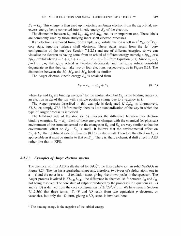
EK � ELI. This energy is then used up in ejecting an Auger electron from the LII orbital, any
excess energy being converted into kinetic energy EA of the electron.
The distinction between LII and LIII, MII and MIII, etc., is an important one. These labels
are commonly used by those studying inner shell electron processes.
If an electron is removed from, for example, a 2p orbital the ion is left in a 2P1=2 or2P3=2
core state, ignoring valence shell electrons. These states result from the 2p5 core
configuration of the ion (see Section 7.1.2.3) and are of different energies, so we can
visualize the electron as having come from an orbital of different energy, namely, a 2p1=2 or a
2p3=2 orbital where j ¼ ‘þ s, ‘þ s� 1; . . . j‘� sj ¼ 32, 12from Equation (7.7). Since mj ¼ j,
j � 1; . . . ;�j the 2p1=2 orbital is two-fold degenerate and the 2p3=2 orbital four-fold
degenerate so that they can take two or four electrons, respectively, as in Figure 8.23. The
distinction between the MI, MII, and MIII labels is similar.
The Auger electron kinetic energy EA is obtained from
EK � ELI¼ E0LII þ EA ð8:15Þ
where EK and ELIare binding energies3 for the neutral atom but E0LII is the binding energy of
an electron in LII of the ion with a single positive charge due to a vacancy in LI.
The Auger process described in this example is designated K–LILII or, alternatively,
KLILII or, simply, KLL. Unfortunately, there is little standardization of the way in which the
type of Auger process is indicated.
The left-hand side of Equation (8.15) involves the difference between two electron
binding energies, EK � ELI. Each of these energies changes with the chemical (or physical)
environment of the atom concerned but the changes in EK and ELIare very similar so that the
environmental effect on EK � ELIis small. It follows that the environmental effect on
E0LII þ EA, the right-hand side of Equation (8.15), is also small. Therefore the effect on EA is
appreciable as it must be similar to that on E0LII . There is, then, a chemical shift effect in AES
rather like that in XPS.
8.2.1.3 Examples of Auger electron spectra
The chemical shift in AES is illustrated for S2O2�3 , the thiosulphate ion, in solid Na2S2O3 in
Figure 8.24. The ion has a tetrahedral shape and, therefore, two types of sulphur atom, one in
a þ 6 and the other in a 7 2 oxidation state, giving rise to two peaks in the spectrum. The
Auger process involved is KLII;IIILII;III, the difference in chemical shift between LII and LIIInot being resolved. The core state of sulphur produced by the processes in Equations (8.12)
and (8.13) is derived from the core configuration 1s22s22p43s2 . . . . We have seen in Section
7.1.2.3(b) that three terms, 1S, 3P and 1D result from two equivalent p electrons, or
vacancies, but only the 1D term, giving a 1D2 state, is involved here.
3 The binding energy is the negative of the orbital energy.
8.2 AUGER ELECTRON AND X-RAY FLUORESCENCE SPECTROSCOPY 319
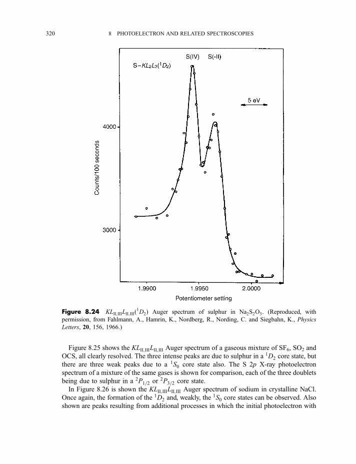
Figure 8.25 shows the KLII;IIILII;III Auger spectrum of a gaseous mixture of SF6, SO2 and
OCS, all clearly resolved. The three intense peaks are due to sulphur in a 1D2 core state, but
there are three weak peaks due to a 1S0 core state also. The S 2p X-ray photoelectron
spectrum of a mixture of the same gases is shown for comparison, each of the three doublets
being due to sulphur in a 2P1=2 or 2P3=2 core state.
In Figure 8.26 is shown the KLII;IIILII;III Auger spectrum of sodium in crystalline NaCl.
Once again, the formation of the 1D2 and, weakly, the1S0 core states can be observed. Also
shown are peaks resulting from additional processes in which the initial photoelectron with
Figure 8.24 KLII;IIILII;IIIð1D2Þ Auger spectrum of sulphur in Na2S2O3. (Reproduced, with
permission, from Fahlmann, A., Hamrin, K., Nordberg, R., Nording, C. and Siegbahn, K., Physics
Letters, 20, 156, 1966.)
320 8 PHOTOELECTRON AND RELATED SPECTROSCOPIES
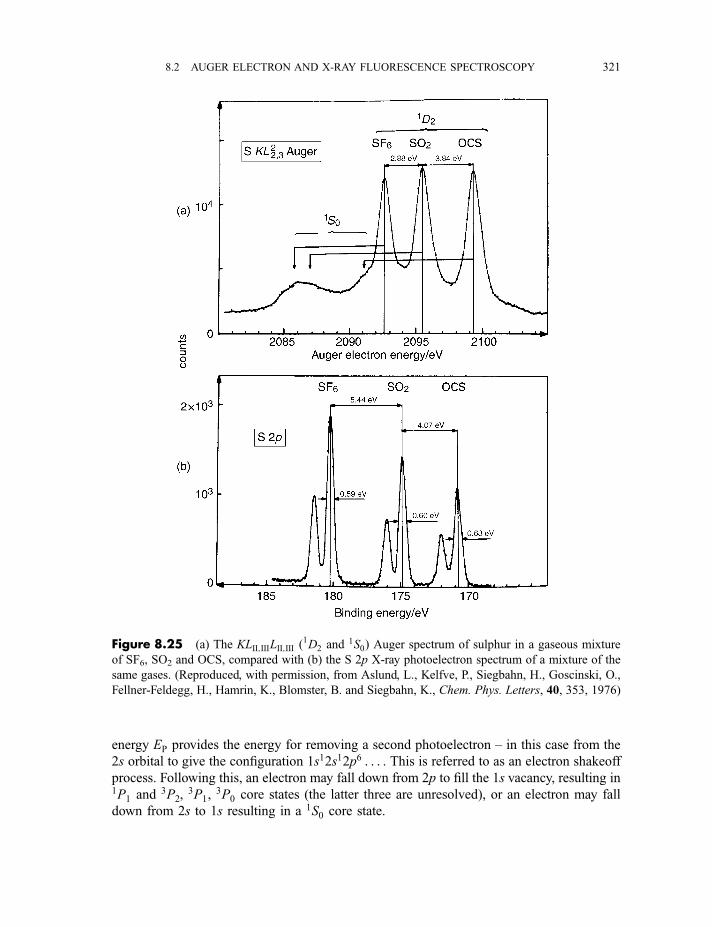
energy EP provides the energy for removing a second photoelectron – in this case from the
2s orbital to give the configuration 1s12s12p6 . . . . This is referred to as an electron shakeoff
process. Following this, an electron may fall down from 2p to fill the 1s vacancy, resulting in1P1 and 3P2,
3P1,3P0 core states (the latter three are unresolved), or an electron may fall
down from 2s to 1s resulting in a 1S0 core state.
Figure 8.25 (a) The KLII;IIILII;III ð1D2 and 1S0Þ Auger spectrum of sulphur in a gaseous mixture
of SF6, SO2 and OCS, compared with (b) the S 2p X-ray photoelectron spectrum of a mixture of the
same gases. (Reproduced, with permission, from Aslund, L., Kelfve, P., Siegbahn, H., Goscinski, O.,
Fellner-Feldegg, H., Hamrin, K., Blomster, B. and Siegbahn, K., Chem. Phys. Letters, 40, 353, 1976)
8.2 AUGER ELECTRON AND X-RAY FLUORESCENCE SPECTROSCOPY 321
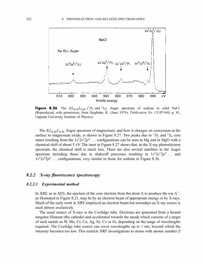
The KLII;IIILII;III Auger spectrum of magnesium, and how it changes on conversion at the
surface to magnesium oxide, is shown in Figure 8.27. Two peaks due to 1D2 and 1S0 core
states resulting from the 1s22s22p4 . . . configurations can be seen in Mg and in MgO with a
chemical shift of about 5 eV. The inset in Figure 8.27 shows that, in the X-ray photoelectron
spectrum, the chemical shift is much less. There are also several satellites in the Auger
spectrum including those due to shakeoff processes resulting in 1s22s12p5 . . . and
1s22s02p6 . . . configurations, very similar to those for sodium in Figure 8.26.
8.2.2 X-ray fluorescence spectroscopy
8.2.2.1 Experimental method
In XRF, as in AES, the ejection of the core electron from the atom A to produce the ion Aþ,as illustrated in Figure 8.21, may be by an electron beam of appropriate energy or by X-rays.
Much of the early work in XRF employed an electron beam but nowadays an X-ray source is
used almost exclusively.
The usual source of X-rays is the Coolidge tube. Electrons are generated from a heated
tungsten filament (the cathode) and accelerated towards the anode which consists of a target
of such metals as W, Mo, Cr, Cu, Ag, Ni, Co or Fe, depending on the range of wavelengths
required. The Coolidge tube source can cover wavelengths up to 1 nm, beyond which the
intensity becomes too low. This restricts XRF investigations to atoms with atomic number Z
Figure 8.26 The KLII;IIILII;III ð1D2 and 1S0Þ Auger spectrum of sodium in solid NaCl.
(Reproduced, with permission, from Siegbahn, K. (June 1976), Publication No. UUIP-940, p. 81,
Uppsala University Institute of Physics)
322 8 PHOTOELECTRON AND RELATED SPECTROSCOPIES
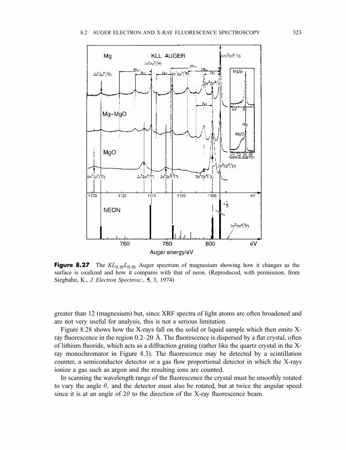
greater than 12 (magnesium) but, since XRF spectra of light atoms are often broadened and
are not very useful for analysis, this is not a serious limitation.
Figure 8.28 shows how the X-rays fall on the solid or liquid sample which then emits X-
ray fluorescence in the region 0.2–20 A. The fluorescence is dispersed by a flat crystal, often
of lithium fluoride, which acts as a diffraction grating (rather like the quartz crystal in the X-
ray monochromator in Figure 8.3). The fluorescence may be detected by a scintillation
counter, a semiconductor detector or a gas flow proportional detector in which the X-rays
ionize a gas such as argon and the resulting ions are counted.
In scanning the wavelength range of the fluorescence the crystal must be smoothly rotated
to vary the angle y; and the detector must also be rotated, but at twice the angular speed
since it is at an angle of 2y to the direction of the X-ray fluorescence beam.
Figure 8.27 The KLII;IIILII;III Auger spectrum of magnesium showing how it changes as the
surface is oxidized and how it compares with that of neon. (Reproduced, with permission, from
Siegbahn, K., J. Electron Spectrosc., 5, 3, 1974)
8.2 AUGER ELECTRON AND X-RAY FLUORESCENCE SPECTROSCOPY 323
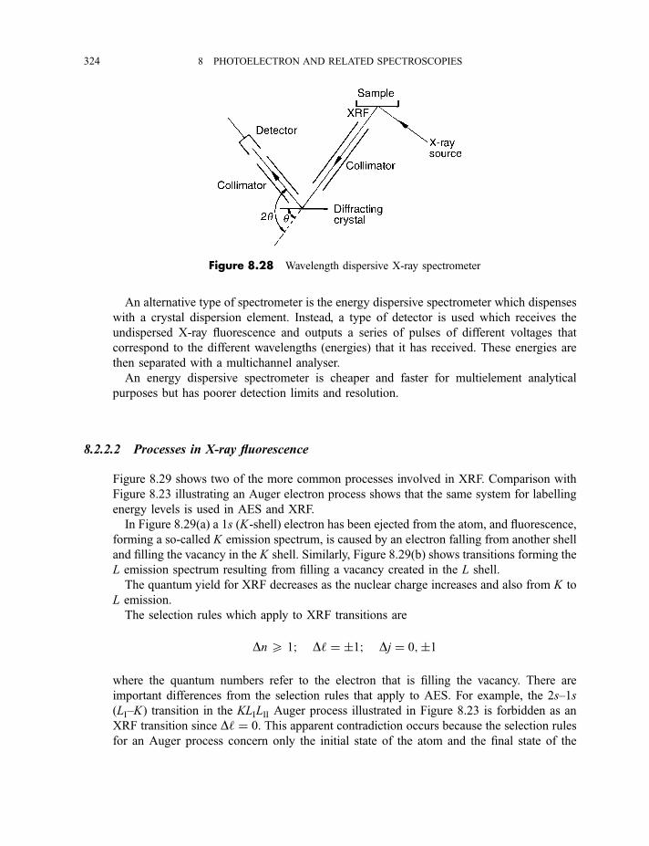
An alternative type of spectrometer is the energy dispersive spectrometer which dispenses
with a crystal dispersion element. Instead, a type of detector is used which receives the
undispersed X-ray fluorescence and outputs a series of pulses of different voltages that
correspond to the different wavelengths (energies) that it has received. These energies are
then separated with a multichannel analyser.
An energy dispersive spectrometer is cheaper and faster for multielement analytical
purposes but has poorer detection limits and resolution.
8.2.2.2 Processes in X-ray fluorescence
Figure 8.29 shows two of the more common processes involved in XRF. Comparison with
Figure 8.23 illustrating an Auger electron process shows that the same system for labelling
energy levels is used in AES and XRF.
In Figure 8.29(a) a 1s (K-shell) electron has been ejected from the atom, and fluorescence,
forming a so-called K emission spectrum, is caused by an electron falling from another shell
and filling the vacancy in the K shell. Similarly, Figure 8.29(b) shows transitions forming the
L emission spectrum resulting from filling a vacancy created in the L shell.
The quantum yield for XRF decreases as the nuclear charge increases and also from K to
L emission.
The selection rules which apply to XRF transitions are
Dn 5 1; D‘ ¼ �1; Dj ¼ 0;�1
where the quantum numbers refer to the electron that is filling the vacancy. There are
important differences from the selection rules that apply to AES. For example, the 2s–1s
(LI–K) transition in the KLILII Auger process illustrated in Figure 8.23 is forbidden as an
XRF transition since D‘ ¼ 0. This apparent contradiction occurs because the selection rules
for an Auger process concern only the initial state of the atom and the final state of the
Figure 8.28 Wavelength dispersive X-ray spectrometer
324 8 PHOTOELECTRON AND RELATED SPECTROSCOPIES
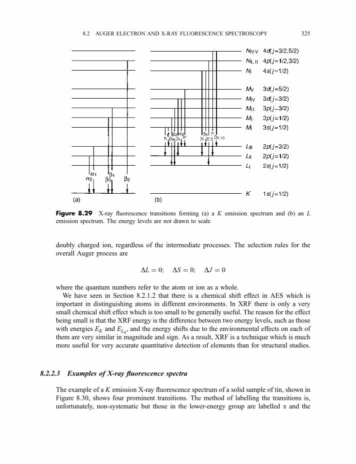
doubly charged ion, regardless of the intermediate processes. The selection rules for the
overall Auger process are
DL ¼ 0; DS ¼ 0; DJ ¼ 0
where the quantum numbers refer to the atom or ion as a whole.
We have seen in Section 8.2.1.2 that there is a chemical shift effect in AES which is
important in distinguishing atoms in different environments. In XRF there is only a very
small chemical shift effect which is too small to be generally useful. The reason for the effect
being small is that the XRF energy is the difference between two energy levels, such as those
with energies EK and ELII, and the energy shifts due to the environmental effects on each of
them are very similar in magnitude and sign. As a result, XRF is a technique which is much
more useful for very accurate quantitative detection of elements than for structural studies.
8.2.2.3 Examples of X-ray fluorescence spectra
The example of a K emission X-ray fluorescence spectrum of a solid sample of tin, shown in
Figure 8.30, shows four prominent transitions. The method of labelling the transitions is,
unfortunately, non-systematic but those in the lower-energy group are labelled a and the
Figure 8.29 X-ray fluorescence transitions forming (a) a K emission spectrum and (b) an L
emission spectrum. The energy levels are not drawn to scale
8.2 AUGER ELECTRON AND X-RAY FLUORESCENCE SPECTROSCOPY 325
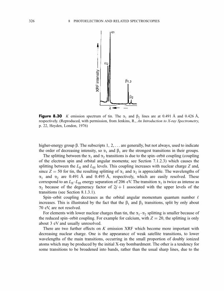
higher-energy group b. The subscripts 1, 2, . . . are generally, but not always, used to indicatethe order of decreasing intensity, so a1 and b1 are the strongest transitions in their groups.
The splitting between the a1 and a2 transitions is due to the spin–orbit coupling (coupling
of the electron spin and orbital angular momenta; see Section 7.1.2.3) which causes the
splitting between the LII and LIII levels. This coupling increases with nuclear charge Z and,
since Z ¼ 50 for tin, the resulting splitting of a1 and a2 is appreciable. The wavelengths ofa1 and a2 are 0.491 A and 0.495 A, respectively, which are easily resolved. These
correspond to an LII–LIII energy separation of 206 eV. The transition a1 is twice as intense asa2 because of the degeneracy factor of 2j þ 1 associated with the upper levels of the
transitions (see Section 8.1.3.1).
Spin–orbit coupling decreases as the orbital angular momentum quantum number ‘increases. This is illustrated by the fact that the b1 and b3 transitions, split by only about
70 eV, are not resolved.
For elements with lower nuclear charges than tin, the a1–a2 splitting is smaller because of
the reduced spin–orbit coupling. For example for calcium, with Z ¼ 20, the splitting is only
about 3 eV and usually unresolved.
There are two further effects on K emission XRF which become more important with
decreasing nuclear charge. One is the appearance of weak satellite transitions, to lower
wavelengths of the main transitions, occurring in the small proportion of doubly ionized
atoms which may be produced by the initial X-ray bombardment. The other is a tendency for
some transitions to be broadened into bands, rather than the usual sharp lines, due to the
Figure 8.30 K emission spectrum of tin. The a1 and b2 lines are at 0.491 A and 0.426 A,
respectively. (Reproduced, with permission, from Jenkins, R., An Introduction to X-ray Spectrometry,
p. 22, Heyden, London, 1976)
326 8 PHOTOELECTRON AND RELATED SPECTROSCOPIES
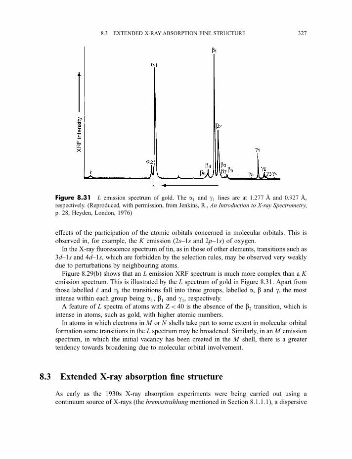
effects of the participation of the atomic orbitals concerned in molecular orbitals. This is
observed in, for example, the K emission (2s–1s and 2p–1s) of oxygen.
In the X-ray fluorescence spectrum of tin, as in those of other elements, transitions such as
3d–1s and 4d–1s, which are forbidden by the selection rules, may be observed very weakly
due to perturbations by neighbouring atoms.
Figure 8.29(b) shows that an L emission XRF spectrum is much more complex than a K
emission spectrum. This is illustrated by the L spectrum of gold in Figure 8.31. Apart from
those labelled ‘ and Z, the transitions fall into three groups, labelled a, b and g, the most
intense within each group being a1, b1 and g1, respectively.A feature of L spectra of atoms with Z< 40 is the absence of the b2 transition, which is
intense in atoms, such as gold, with higher atomic numbers.
In atoms in which electrons in M or N shells take part to some extent in molecular orbital
formation some transitions in the L spectrum may be broadened. Similarly, in anM emission
spectrum, in which the initial vacancy has been created in the M shell, there is a greater
tendency towards broadening due to molecular orbital involvement.
8.3 Extended X-ray absorption fine structure
As early as the 1930s X-ray absorption experiments were being carried out using a
continuum source of X-rays (the bremsstrahlung mentioned in Section 8.1.1.1), a dispersive
Figure 8.31 L emission spectrum of gold. The a1 and g1 lines are at 1.277 A and 0.927 A,
respectively. (Reproduced, with permission, from Jenkins, R., An Introduction to X-ray Spectrometry,
p. 28, Heyden, London, 1976)
8.3 EXTENDED X-RAY ABSORPTION FINE STRUCTURE 327
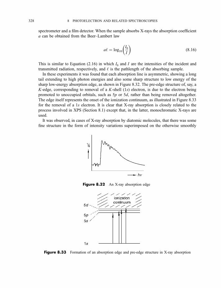
spectrometer and a film detector. When the sample absorbs X-rays the absorption coefficient
a can be obtained from the Beer–Lambert law
a‘ ¼ log10I0
I
� �ð8:16Þ
This is similar to Equation (2.16) in which I0 and I are the intensities of the incident and
transmitted radiation, respectively, and ‘ is the pathlength of the absorbing sample.
In these experiments it was found that each absorption line is asymmetric, showing a long
tail extending to high photon energies and also some sharp structure to low energy of the
sharp low-energy absorption edge, as shown in Figure 8.32. The pre-edge structure of, say, a
K-edge, corresponding to removal of a K-shell (1s) electron, is due to the electron being
promoted to unoccupied orbitals, such as 5p or 5d, rather than being removed altogether.
The edge itself represents the onset of the ionization continuum, as illustrated in Figure 8.33
for the removal of a 1s electron. It is clear that X-ray absorption is closely related to the
process involved in XPS (Section 8.1) except that, in the latter, monochromatic X-rays are
used.
It was observed, in cases of X-ray absorption by diatomic molecules, that there was some
fine structure in the form of intensity variations superimposed on the otherwise smoothly
Figure 8.32 An X-ray absorption edge
Figure 8.33 Formation of an absorption edge and pre-edge structure in X-ray absorption
328 8 PHOTOELECTRON AND RELATED SPECTROSCOPIES
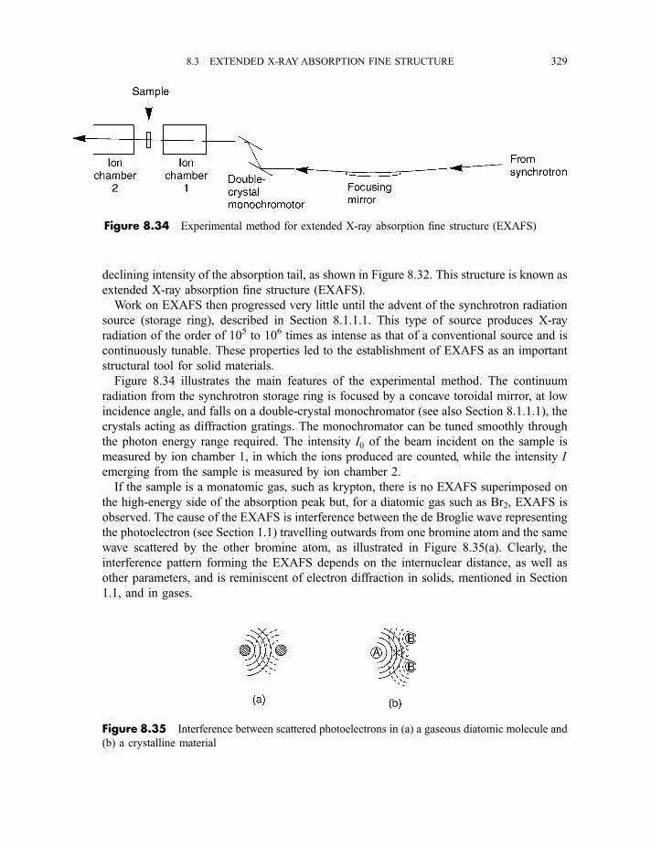
declining intensity of the absorption tail, as shown in Figure 8.32. This structure is known as
extended X-ray absorption fine structure (EXAFS).
Work on EXAFS then progressed very little until the advent of the synchrotron radiation
source (storage ring), described in Section 8.1.1.1. This type of source produces X-ray
radiation of the order of 105 to 106 times as intense as that of a conventional source and is
continuously tunable. These properties led to the establishment of EXAFS as an important
structural tool for solid materials.
Figure 8.34 illustrates the main features of the experimental method. The continuum
radiation from the synchrotron storage ring is focused by a concave toroidal mirror, at low
incidence angle, and falls on a double-crystal monochromator (see also Section 8.1.1.1), the
crystals acting as diffraction gratings. The monochromator can be tuned smoothly through
the photon energy range required. The intensity I0 of the beam incident on the sample is
measured by ion chamber 1, in which the ions produced are counted, while the intensity I
emerging from the sample is measured by ion chamber 2.
If the sample is a monatomic gas, such as krypton, there is no EXAFS superimposed on
the high-energy side of the absorption peak but, for a diatomic gas such as Br2, EXAFS is
observed. The cause of the EXAFS is interference between the de Broglie wave representing
the photoelectron (see Section 1.1) travelling outwards from one bromine atom and the same
wave scattered by the other bromine atom, as illustrated in Figure 8.35(a). Clearly, the
interference pattern forming the EXAFS depends on the internuclear distance, as well as
other parameters, and is reminiscent of electron diffraction in solids, mentioned in Section
1.1, and in gases.
Figure 8.34 Experimental method for extended X-ray absorption fine structure (EXAFS)
Figure 8.35 Interference between scattered photoelectrons in (a) a gaseous diatomic molecule and
(b) a crystalline material
8.3 EXTENDED X-RAY ABSORPTION FINE STRUCTURE 329
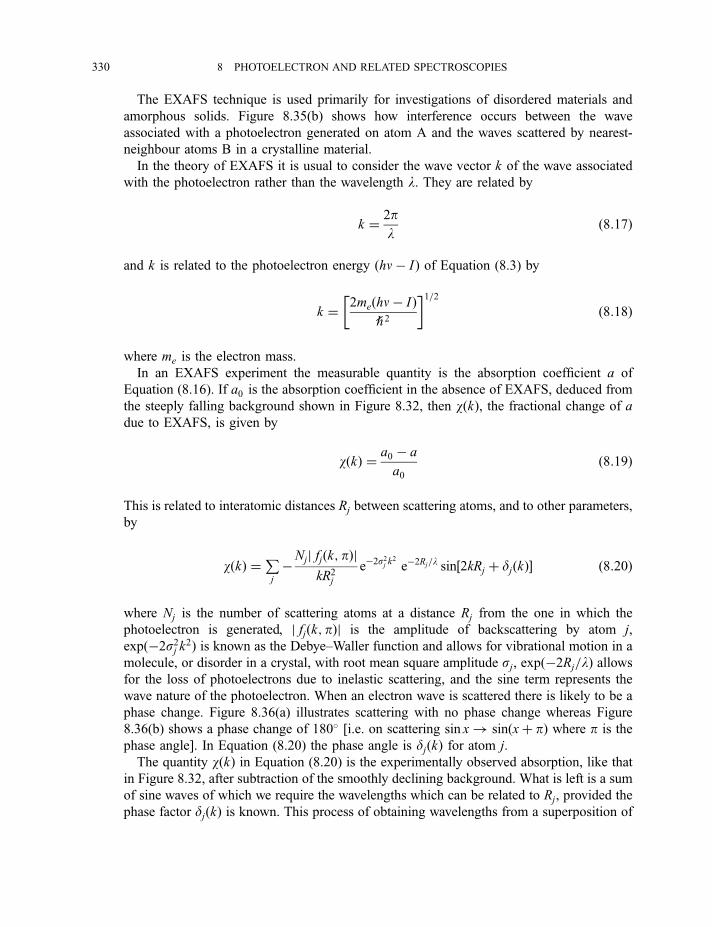
The EXAFS technique is used primarily for investigations of disordered materials and
amorphous solids. Figure 8.35(b) shows how interference occurs between the wave
associated with a photoelectron generated on atom A and the waves scattered by nearest-
neighbour atoms B in a crystalline material.
In the theory of EXAFS it is usual to consider the wave vector k of the wave associated
with the photoelectron rather than the wavelength l. They are related by
k ¼ 2pl
ð8:17Þ
and k is related to the photoelectron energy ðhn� I Þ of Equation (8.3) by
k ¼ 2meðhn� I Þh2
� �1=2ð8:18Þ
where me is the electron mass.
In an EXAFS experiment the measurable quantity is the absorption coefficient a of
Equation (8.16). If a0 is the absorption coefficient in the absence of EXAFS, deduced from
the steeply falling background shown in Figure 8.32, then wðkÞ, the fractional change of a
due to EXAFS, is given by
wðkÞ ¼ a0 � a
a0ð8:19Þ
This is related to interatomic distances Rj between scattering atoms, and to other parameters,
by
wðkÞ ¼Pj
�Njj fjðk; pÞjkR2
j
e�2s2j k
2
e�2Rj=l sin½2kRj þ djðkÞ� ð8:20Þ
where Nj is the number of scattering atoms at a distance Rj from the one in which the
photoelectron is generated, j fjðk; pÞj is the amplitude of backscattering by atom j,
expð�2s2j k2Þ is known as the Debye–Waller function and allows for vibrational motion in a
molecule, or disorder in a crystal, with root mean square amplitude sj, expð�2Rj=lÞ allowsfor the loss of photoelectrons due to inelastic scattering, and the sine term represents the
wave nature of the photoelectron. When an electron wave is scattered there is likely to be a
phase change. Figure 8.36(a) illustrates scattering with no phase change whereas Figure
8.36(b) shows a phase change of 180� [i.e. on scattering sin x! sinðxþ pÞ where p is the
phase angle]. In Equation (8.20) the phase angle is djðkÞ for atom j.
The quantity wðkÞ in Equation (8.20) is the experimentally observed absorption, like that
in Figure 8.32, after subtraction of the smoothly declining background. What is left is a sum
of sine waves of which we require the wavelengths which can be related to Rj, provided the
phase factor djðkÞ is known. This process of obtaining wavelengths from a superposition of
330 8 PHOTOELECTRON AND RELATED SPECTROSCOPIES
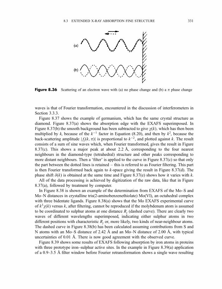
waves is that of Fourier transformation, encountered in the discussion of interferometers in
Section 3.3.3.
Figure 8.37 shows the example of germanium, which has the same crystal structure as
diamond. Figure 8.37(a) shows the absorption edge with the EXAFS superimposed. In
Figure 8.37(b) the smooth background has been subtracted to give wðkÞ;which has then beenmultiplied by k, because of the k�1 factor in Equation (8.20), and then by k2, because the
back-scattering amplitude j fjðk; pÞj is proportional to k�2, and plotted against k. The result
consists of a sum of sine waves which, when Fourier transformed, gives the result in Figure
8.37(c). This shows a major peak at about 2.2 A, corresponding to the four nearest
neighbours in the diamond-type (tetrahedral) structure and other peaks corresponding to
more distant neighbours. Then a ‘filter’ is applied to the curve in Figure 8.37(c) so that only
the part between the dotted lines is retained – this is referred to as Fourier filtering. This part
is then Fourier transformed back again to k-space giving the result in Figure 8.37(d). The
phase shift dðkÞ is obtained at the same time and Figure 8.37(e) shows how it varies with k.
All of the data processing is achieved by digitization of the raw data, like that in Figure
8.37(a), followed by treatment by computer.
In Figure 8.38 is shown an example of the determination from EXAFS of the Mo–S and
Mo–N distances in crystalline tris(2-aminobenzenethiolate) Mo(VI), an octahedral complex
with three bidentate ligands. Figure 8.38(a) shows that the Mo EXAFS experimental curve
of k3wðkÞ versus k, after filtering, cannot be reproduced if the molybdenum atom is assumed
to be coordinated to sulphur atoms at one distance Rj (dashed curve). There are clearly two
waves of different wavelengths superimposed, indicating either sulphur atoms in two
different positions with characteristic Rj or, more likely, two kinds of near-neighbour atoms.
The dashed curve in Figure 8.38(b) has been calculated assuming contributions from S and
N atoms with an Mo–S distance of 2.42 A and an Mo–N distance of 2.00 A, with typical
uncertainties of 0.01 A. There is now good agreement with the observed curve.
Figure 8.39 shows some results of EXAFS following absorption by iron atoms in proteins
with three prototype iron–sulphur active sites. In the example in Figure 8.39(a) application
of a 0.9–3.5 A filter window before Fourier retransformation shows a single wave resulting
Figure 8.36 Scattering of an electron wave with (a) no phase change and (b) a p phase change
8.3 EXTENDED X-RAY ABSORPTION FINE STRUCTURE 331
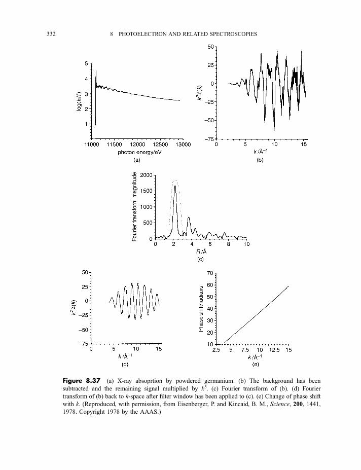
Figure 8.37 (a) X-ray absoprtion by powdered germanium. (b) The background has been
subtracted and the remaining signal multiplied by k3. (c) Fourier transform of (b). (d) Fourier
transform of (b) back to k-space after filter window has been applied to (c). (e) Change of phase shift
with k. (Reproduced, with permission, from Eisenberger, P. and Kincaid, B. M., Science, 200, 1441,
1978. Copyright 1978 by the AAAS.)
332 8 PHOTOELECTRON AND RELATED SPECTROSCOPIES
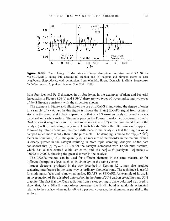
from four identical Fe–S distances in a rubredoxin. In the examples of plant and bacterial
ferredoxins in Figures 8.39(b) and 8.39(c) there are two types of waves indicating two types
of Fe–S linkage consistent with the structures shown.
The example in Figure 8.40 illustrates the use of EXAFS in indicating the degree of order
in a sample of a catalyst. In this figure is shown the k3wðkÞ EXAFS signal from osmium
atoms in the pure metal to be compared with that of a 1% osmium catalyst in small clusters
dispersed on a silica surface. The main peak in the Fourier transformed spectrum is due to
Os–Os nearest neighbours and is much more intense (ca 3.2) in the pure metal than in the
catalyst (ca 0.8), indicating many more Os–Os bonds. When the filter window is applied,
followed by retransformation, the main difference in the catalyst is that the single wave is
damped much more rapidly than in the pure metal. The damping is due to the expð�2s2j k2Þfactor in Equation (8.20). The quantity sj is a measure of the disorder in the material which
is clearly greater in the catalyst resulting in more rapid damping. Analysis of the data
has shown that (a) N1 ¼ 8:3� 2:0 for the catalyst, compared with 12 for pure osmium,
which has a face-centred cubic structure, and (b) Ds21 ¼ s21 ðcatalystÞ � s21 metalÞ ¼0:0022� 0:0002, showing the great disorder in the catalyst.
The EXAFS method can be used for different elements in the same material or for
different absorption edges, such as 1s, 2s or 2p, in the same element.
Auger electrons, produced in the way described in Section 8.2.1, may also produce
scattering interference in the same way as ordinary photoelectrons. The technique is useful
for studying surfaces and is known as surface EXAFS, or SEXAFS. An example of its use is
an investigation of Br2 adsorbed onto carbon in the form of 50% carbon crystallites and 50%
graphite. The fact that the X-ray radiation from a storage ring is plane polarized was used to
show that, for a 20% Br2 monolayer coverage, the Br–Br bond is randomly orientated
relative to the surface whereas, for 60 to 90 per cent coverage, the alignment is parallel to the
surface.
Figure 8.38 Curve fitting of Mo extended X-ray absorption fine structure (EXAFS) for
Mo(SC6H4NH)3, taking into account (a) sulphur and (b) sulphur and nitrogen atoms as near
neighbours. (Reproduced, with permission, from Winnick, H. and Doniach, S. (Eds), Synchrotron
Radiation Research, p. 436, Plenum, New York, 1980)
8.3 EXTENDED X-RAY ABSORPTION FINE STRUCTURE 333
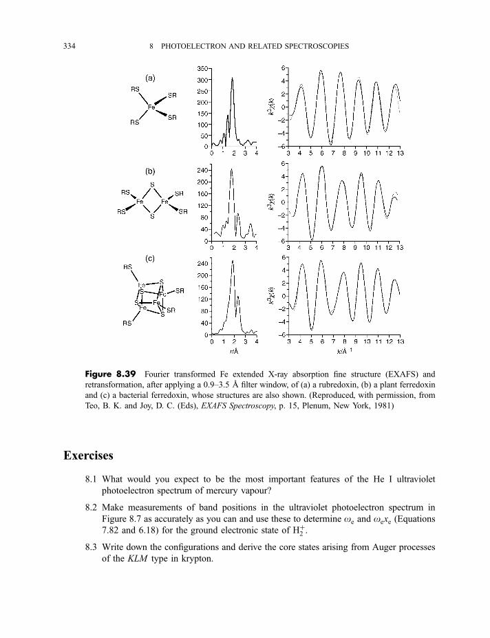
Exercises
8.1 What would you expect to be the most important features of the He I ultraviolet
photoelectron spectrum of mercury vapour?
8.2 Make measurements of band positions in the ultraviolet photoelectron spectrum in
Figure 8.7 as accurately as you can and use these to determine oe and oexe (Equations
7.82 and 6.18) for the ground electronic state of Hþ2 .
8.3 Write down the configurations and derive the core states arising from Auger processes
of the KLM type in krypton.
Figure 8.39 Fourier transformed Fe extended X-ray absorption fine structure (EXAFS) and
retransformation, after applying a 0.9–3.5 A filter window, of (a) a rubredoxin, (b) a plant ferredoxin
and (c) a bacterial ferredoxin, whose structures are also shown. (Reproduced, with permission, from
Teo, B. K. and Joy, D. C. (Eds), EXAFS Spectroscopy, p. 15, Plenum, New York, 1981)
334 8 PHOTOELECTRON AND RELATED SPECTROSCOPIES
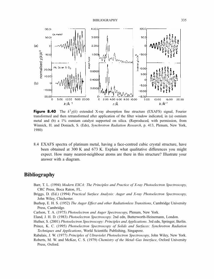
8.4 EXAFS spectra of platinum metal, having a face-centred cubic crystal structure, have
been obtained at 300 K and 673 K. Explain what qualitative differences you might
expect. How many nearest-neighbour atoms are there in this structure? Illustrate your
answer with a diagram.
Bibliography
Barr, T. L. (1994) Modern ESCA: The Principles and Practice of X-ray Photoelectron Spectroscopy,
CRC Press, Boca Raton, FL.
Briggs, D. (Ed.) (1994) Practical Surface Analysis: Auger and X-ray Photoelectron Spectroscopy,
John Wiley, Chichester.
Burhop, E. H. S. (1952) The Auger Effect and other Radiationless Transitions, Cambridge University
Press, Cambridge.
Carlson, T. A. (1975) Photoelectron and Auger Spectroscopy, Plenum, New York.
Eland, J. H. D. (1983) Photoelectron Spectroscopy. 2nd edn, Butterworth-Heinemann, London.
Hufner, S. (2001) Photoelectron Spectroscopy: Principles and Applications. 3rd edn, Springer, Berlin.
Prince, K. C. (1995) Photoelectron Spectroscopy of Solids and Surfaces: Synchrotron Radiation
Techniques and Applications, World Scientific Publishing, Singapore.
Rabalais, J. W. (1977) Principles of Ultraviolet Photoelectron Spectroscopy, John Wiley, New York.
Roberts, M. W. and McKee, C. S. (1979) Chemistry of the Metal–Gas Interface, Oxford University
Press, Oxford.
Figure 8.40 The k3wðkÞ extended X-ray absorption fine structure (EXAFS) signal, Fourier
transformed and then retransformed after application of the filter window indicated, in (a) osmium
metal and (b) a 1% osmium catalyst supported on silica. (Reproduced, with permission, from
Winnick, H. and Doniach, S. (Eds), Synchrotron Radiation Research, p. 413, Plenum, New York,
1980)
BIBLIOGRAPHY 335

Siegbahn, K., Nordling, C., Fahlman, A., Nordberg, R., Hamerin, K., Hedman, J., Johansson, G.,
Bergmark, T., Karlsson, S.-E., Lindgren, I. and Lindberg, B. (1967) Electron Spectroscopy for
Chemical Analysis: Atomic, Molecular, and Solid State Structure Studies by Means of Electron
Spectroscopy, Almqvist and Wiksells, Uppsala.
Teo, B. (1986) EXAFS: Basic Principles and Data Analysis, Springer, Berlin.
Turner, D. W., Baker, C., Baker, A. D. and Brundle, C. R. (1970). Molecular Photoelectron
Spectroscopy, John Wiley, Chichester.
Winnick, H. and Doniach, S. (Eds) (1980) Synchrotron Radiation Research, Plenum, New York.
336 8 PHOTOELECTRON AND RELATED SPECTROSCOPIES
9LASERS AND LASERSPECTROSCOPY
9.1 General discussion of lasers
9.1.1 General features and properties
The word ‘laser’ is an acronym derived from ‘light amplification by the stimulated emission
of radiation’. If the light concerned is in the microwave region then the alternative acronym
‘maser’ is often used. Although the first such device to be constructed was the ammonia
maser in 1954 it is the lasers made subsequently which operate in the infrared, visible or
ultraviolet regions of the spectrum which have made a greater impact.
In Section 2.2 we saw that emission of radiation by an excited atom or molecule M* may
be by a spontaneous (Equation 2.4) or by an induced, or stimulated, process
M*þ hc~nn! Mþ 2hc~nn ð9:1Þ
as in Equation (2.5).
Laser radiation is emitted entirely by the process of stimulated emission, unlike the more
conventional sources of radiation discussed in Chapter 3, which emit through a spontaneous
process.
For induced emission from the upper energy level n of the two-level system in Figure
2.2(a) to dominate absorption (Equation 2.3) there must be a population inversion between
the two levels, that is Nn > Nm where Ni refers to the population of state i. To disturb the
normal Boltzmann population distribution (Equation 2.11), in which Nn < Nm, requires an
input of energy. The process by which such a population inversion is brought about is known
as pumping. A system, which may be gaseous, solid or liquid and in which a population
inversion has been created is referred to as an active medium. According to Equation (9.1)
the active medium is capable of acting as an amplifier of radiation falling on it. The equation
shows that, for every photon entering the active medium, two photons are emitted from it.
To make an oscillator from an amplifier requires, in the language of electronics, positive
feedback. In lasers this is provided by the active medium being between two mirrors, both of
them highly reflecting but one rather less so in order to allow some of the stimulated
radiation to leak out and form the laser beam. The region bounded by the mirrors is called
the laser cavity. Various mirror systems are used but that shown in Figure 9.1, consisting of
337
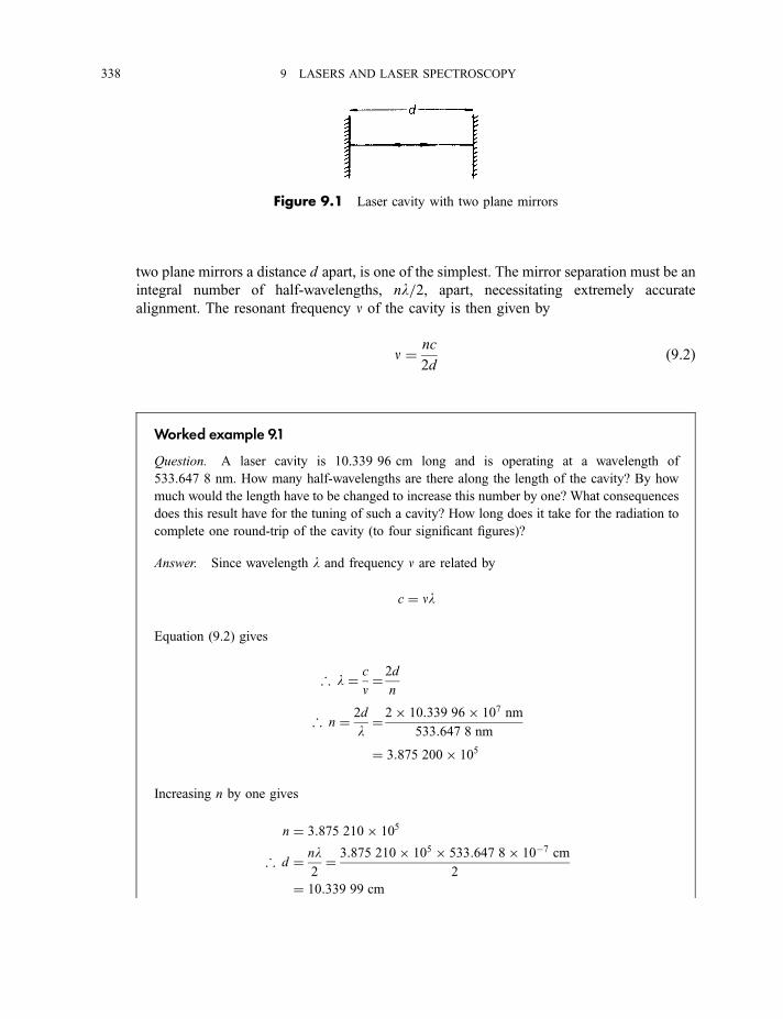
two plane mirrors a distance d apart, is one of the simplest. The mirror separation must be an
integral number of half-wavelengths, nl=2, apart, necessitating extremely accurate
alignment. The resonant frequency n of the cavity is then given by
n ¼ nc
2dð9:2Þ
Worked example 9.1
Question. A laser cavity is 10.339 96 cm long and is operating at a wavelength of
533.647 8 nm. How many half-wavelengths are there along the length of the cavity? By how
much would the length have to be changed to increase this number by one? What consequences
does this result have for the tuning of such a cavity? How long does it take for the radiation to
complete one round-trip of the cavity (to four significant figures)?
Answer. Since wavelength l and frequency n are related by
c ¼ nl
Equation (9.2) gives
; l ¼ c
n¼ 2d
n
; n ¼ 2d
l¼ 2� 10:339 96� 107 nm
533:647 8 nm
¼ 3:875 200� 105
Increasing n by one gives
n ¼ 3:875 210� 105
; d ¼ nl2¼ 3:875 210� 105 � 533:647 8� 10�7 cm
2
¼ 10:339 99 cm
Figure 9.1 Laser cavity with two plane mirrors
338 9 LASERS AND LASER SPECTROSCOPY
Therefore the cavity has been increased in length by 0.000 03 cm¼ 0.3 mm. This means that to
tune the cavity to a half wavelength of the radiation requires an extremely accurate movement of
one of the mirrors forming the cavity.
One round-trip of the cavity covers a distance of 20.680 cm
; time taken ¼ 20:680 cm
2:997 9� 1010 cm s�1
¼ 6:898� 10�10 s
The reflecting surfaces of the mirrors are specially coated, with alternate layers of high
and low dielectric materials such as TiO2 and SiO, to give almost total reflection at the
specific laser wavelength. The usual aluminium, silver or gold coatings are not sufficiently
highly reflecting. One of the mirrors is coated so as to allow 1 to 10 per cent of the radiation
to emerge as the laser beam.
Photons of energy hc~nn are generated initially in the cavity through spontaneous emission.
Those that strike the cavity mirrors at 90� are retained within the cavity causing the photon
flux to reach a level which is sufficiently high to cause stimulated emission to occur, and the
active medium is said to lase.
Laser radiation has four very remarkable properties:
1. Directionality. The laser beam emerging from the output mirror of the cavity is highly
parallel, which is a consequence of the strict requirements for the alignment of the cavity
mirrors. Divergence of the beam is typically a few milliradians.
2. Monochromaticity. If the energy levels n and m in Figure 2.2(a) are sharp, as they are in
a gaseous active medium, the Planck relation of Equation (2.2) limits the wavelength
range of the radiation. However, whatever the nature of the active medium, the fact that
the laser cavity is resonant only for the frequencies given by Equation (9.2) limits the
wavelength range.
3. Brightness. This is defined as the power emitted per unit area of the output mirror per
unit solid angle and is extremely high compared with that of a conventional source. The
reason for this is that, although the power may be only modest, as in, for example, a
0.5 mW helium–neon gas laser, the solid angle over which it is distributed is very small.
4. Coherence. Conventional sources of radiation are incoherent, which means that the
electromagnetic waves associated with any two photons of the same wavelength are, in
general, out of phase. The coherence of laser radiation is both temporal and spatial, the
coherence lasting for a relatively long time and extending over a relatively large distance.
Coherence of laser radiation is responsible for its use as a source of intense local heating,
as in metal cutting and welding, and for holography.
9.1 GENERAL DISCUSSION OF LASERS 339
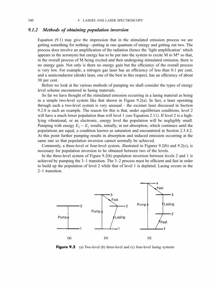
9.1.2 Methods of obtaining population inversion
Equation (9.1) may give the impression that in the stimulated emission process we are
getting something for nothing—putting in one quantum of energy and getting out two. The
process does involve an amplification of the radiation (hence the ‘light amplification’ which
appears in the acronym) but energy has to be put into the system to excite M to M* so that,
in the overall process of M being excited and then undergoing stimulated emission, there is
no energy gain. Not only is there no energy gain but the efficiency of the overall process
is very low. For example, a nitrogen gas laser has an efficiency of less than 0.1 per cent,
and a semiconductor (diode) laser, one of the best in this respect, has an efficiency of about
30 per cent.
Before we look at the various methods of pumping we shall consider the types of energy
level scheme encountered in lasing materials.
So far we have thought of the stimulated emission occurring in a lasing material as being
in a simple two-level system like that shown in Figure 9.2(a). In fact, a laser operating
through such a two-level system is very unusual – the excimer laser discussed in Section
9.2.8 is such an example. The reason for this is that, under equilibrium conditions, level 2
will have a much lower population than will level 1 (see Equation 2.11). If level 2 is a high-
lying vibrational, or an electronic, energy level the population will be negligibly small.
Pumping with energy E2 � E1 results, initially, in net absorption, which continues until the
populations are equal, a condition known as saturation and encountered in Section 2.3.4.2.
At this point further pumping results in absorption and induced emission occurring at the
same rate so that population inversion cannot normally be achieved.
Commonly, a three-level or four-level system, illustrated in Figures 9.2(b) and 9.2(c), is
necessary for population inversion to be obtained between two of the levels.
In the three-level system of Figure 9.2(b) population inversion between levels 2 and 1 is
achieved by pumping the 3–1 transition. The 3–2 process must be efficient and fast in order
to build up the population of level 2 while that of level 1 is depleted. Lasing occurs in the
2–1 transition.
Figure 9.2 (a) Two-level (b) three-level and (c) four-level lasing systems
340 9 LASERS AND LASER SPECTROSCOPY
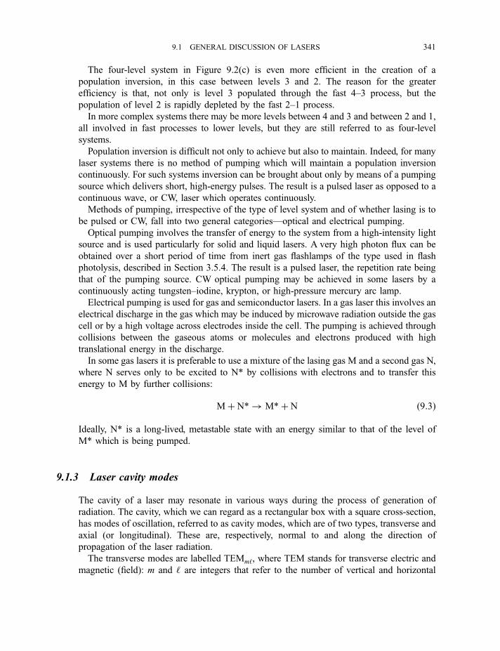
The four-level system in Figure 9.2(c) is even more efficient in the creation of a
population inversion, in this case between levels 3 and 2. The reason for the greater
efficiency is that, not only is level 3 populated through the fast 4–3 process, but the
population of level 2 is rapidly depleted by the fast 2–1 process.
In more complex systems there may be more levels between 4 and 3 and between 2 and 1,
all involved in fast processes to lower levels, but they are still referred to as four-level
systems.
Population inversion is difficult not only to achieve but also to maintain. Indeed, for many
laser systems there is no method of pumping which will maintain a population inversion
continuously. For such systems inversion can be brought about only by means of a pumping
source which delivers short, high-energy pulses. The result is a pulsed laser as opposed to a
continuous wave, or CW, laser which operates continuously.
Methods of pumping, irrespective of the type of level system and of whether lasing is to
be pulsed or CW, fall into two general categories—optical and electrical pumping.
Optical pumping involves the transfer of energy to the system from a high-intensity light
source and is used particularly for solid and liquid lasers. A very high photon flux can be
obtained over a short period of time from inert gas flashlamps of the type used in flash
photolysis, described in Section 3.5.4. The result is a pulsed laser, the repetition rate being
that of the pumping source. CW optical pumping may be achieved in some lasers by a
continuously acting tungsten–iodine, krypton, or high-pressure mercury arc lamp.
Electrical pumping is used for gas and semiconductor lasers. In a gas laser this involves an
electrical discharge in the gas which may be induced by microwave radiation outside the gas
cell or by a high voltage across electrodes inside the cell. The pumping is achieved through
collisions between the gaseous atoms or molecules and electrons produced with high
translational energy in the discharge.
In some gas lasers it is preferable to use a mixture of the lasing gas M and a second gas N,
where N serves only to be excited to N* by collisions with electrons and to transfer this
energy to M by further collisions:
Mþ N*! M*þ N ð9:3Þ
Ideally, N* is a long-lived, metastable state with an energy similar to that of the level of
M* which is being pumped.
9.1.3 Laser cavity modes
The cavity of a laser may resonate in various ways during the process of generation of
radiation. The cavity, which we can regard as a rectangular box with a square cross-section,
has modes of oscillation, referred to as cavity modes, which are of two types, transverse and
axial (or longitudinal). These are, respectively, normal to and along the direction of
propagation of the laser radiation.
The transverse modes are labelled TEMm‘, where TEM stands for transverse electric and
magnetic (field): m and ‘ are integers that refer to the number of vertical and horizontal
9.1 GENERAL DISCUSSION OF LASERS 341
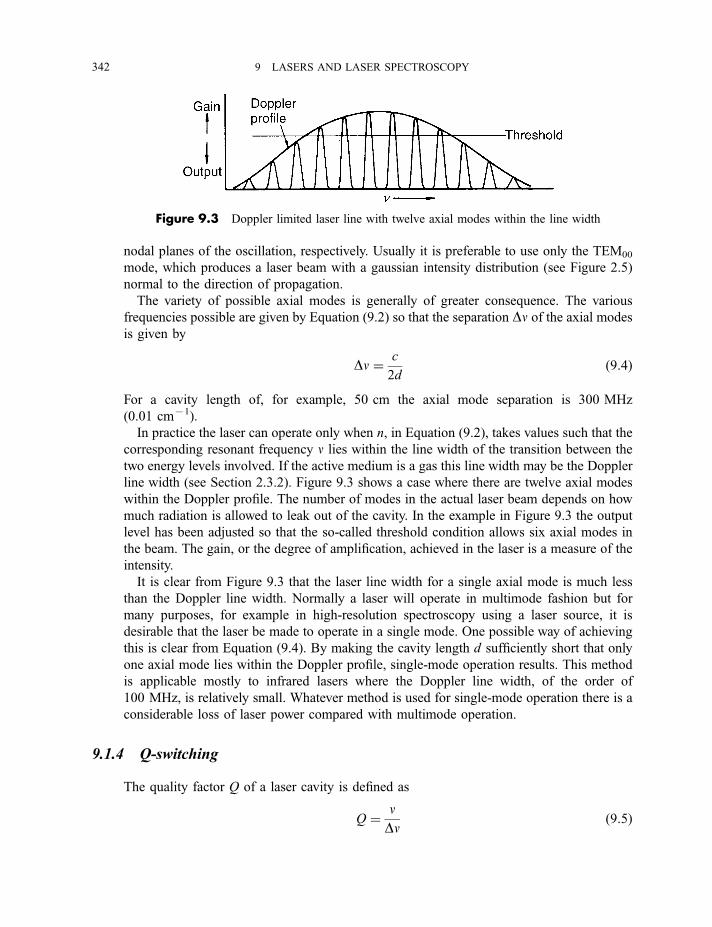
nodal planes of the oscillation, respectively. Usually it is preferable to use only the TEM00
mode, which produces a laser beam with a gaussian intensity distribution (see Figure 2.5)
normal to the direction of propagation.
The variety of possible axial modes is generally of greater consequence. The various
frequencies possible are given by Equation (9.2) so that the separation Dn of the axial modes
is given by
Dn ¼ c
2dð9:4Þ
For a cavity length of, for example, 50 cm the axial mode separation is 300 MHz
(0.01 cm71).
In practice the laser can operate only when n, in Equation (9.2), takes values such that the
corresponding resonant frequency n lies within the line width of the transition between the
two energy levels involved. If the active medium is a gas this line width may be the Doppler
line width (see Section 2.3.2). Figure 9.3 shows a case where there are twelve axial modes
within the Doppler profile. The number of modes in the actual laser beam depends on how
much radiation is allowed to leak out of the cavity. In the example in Figure 9.3 the output
level has been adjusted so that the so-called threshold condition allows six axial modes in
the beam. The gain, or the degree of amplification, achieved in the laser is a measure of the
intensity.
It is clear from Figure 9.3 that the laser line width for a single axial mode is much less
than the Doppler line width. Normally a laser will operate in multimode fashion but for
many purposes, for example in high-resolution spectroscopy using a laser source, it is
desirable that the laser be made to operate in a single mode. One possible way of achieving
this is clear from Equation (9.4). By making the cavity length d sufficiently short that only
one axial mode lies within the Doppler profile, single-mode operation results. This method
is applicable mostly to infrared lasers where the Doppler line width, of the order of
100 MHz, is relatively small. Whatever method is used for single-mode operation there is a
considerable loss of laser power compared with multimode operation.
9.1.4 Q-switching
The quality factor Q of a laser cavity is defined as
Q ¼ nDn
ð9:5Þ
Figure 9.3 Doppler limited laser line with twelve axial modes within the line width
342 9 LASERS AND LASER SPECTROSCOPY
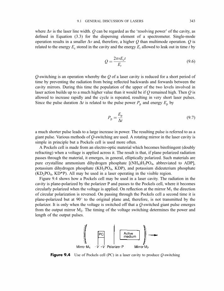
where Dn is the laser line width. Q can be regarded as the ‘resolving power’ of the cavity, as
defined in Equation (3.3) for the dispersing element of a spectrometer. Single-mode
operation results in a smaller Dn and, therefore, a higher Q than multimode operation. Q is
related to the energy Ec stored in the cavity and the energy Et allowed to leak out in time t by
Q ¼ 2pnEct
Et
ð9:6Þ
Q-switching is an operation whereby the Q of a laser cavity is reduced for a short period of
time by preventing the radiation from being reflected backwards and forwards between the
cavity mirrors. During this time the population of the upper of the two levels involved in
laser action builds up to a much higher value than it would be if Q remained high. Then Q is
allowed to increase rapidly and the cycle is repeated, resulting in very short laser pulses.
Since the pulse duration Dt is related to the pulse power Pp and energy Ep by
Pp ¼Ep
Dtð9:7Þ
a much shorter pulse leads to a large increase in power. The resulting pulse is referred to as a
giant pulse. Various methods of Q-switching are used. A rotating mirror in the laser cavity is
simple in principle but a Pockels cell is used more often.
A Pockels cell is made from an electro-optic material which becomes birefringent (doubly
refracting) when a voltage is applied across it. The result is that, if plane polarized radiation
passes through the material, it emerges, in general, elliptically polarized. Such materials are
pure crystalline ammonium dihydrogen phosphate [(NH4)H2PO4, abbreviated to ADP],
potassium dihydrogen phosphate (KH2PO4, KDP), and potassium dideuterium phosphate
(KD2PO4, KD*P). All may be used in a laser operating in the visible region.
Figure 9.4 shows how a Pockels cell may be used in a laser cavity. The radiation in the
cavity is plane-polarized by the polarizer P and passes to the Pockels cell, where it becomes
circularly polarized when the voltage is applied. On reflection at the mirror M1 the direction
of circular polarization is reversed. On passing through the Pockels cell a second time it is
plane-polarized but at 90� to the original plane and, therefore, is not transmitted by the
polarizer. It is only when the voltage is switched off that a Q-switched giant pulse emerges
from the output mirror M2. The timing of the voltage switching determines the power and
length of the output pulses.
Figure 9.4 Use of Pockels cell (PC) in a laser cavity to produce Q-switching
9.1 GENERAL DISCUSSION OF LASERS 343
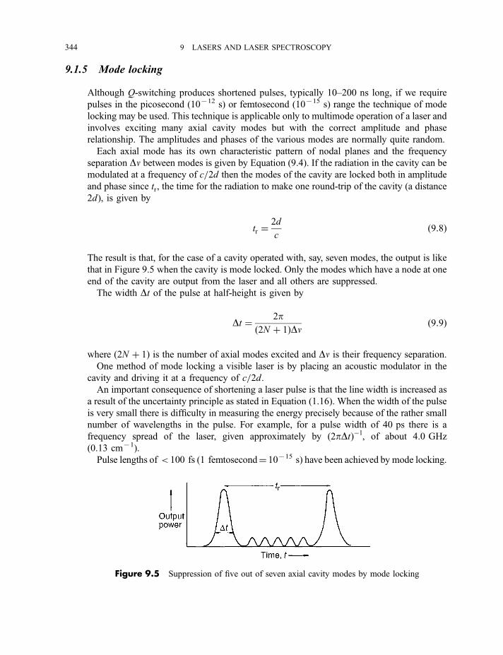
9.1.5 Mode locking
Although Q-switching produces shortened pulses, typically 10–200 ns long, if we require
pulses in the picosecond (10712 s) or femtosecond (10715 s) range the technique of mode
locking may be used. This technique is applicable only to multimode operation of a laser and
involves exciting many axial cavity modes but with the correct amplitude and phase
relationship. The amplitudes and phases of the various modes are normally quite random.
Each axial mode has its own characteristic pattern of nodal planes and the frequency
separation Dn between modes is given by Equation (9.4). If the radiation in the cavity can be
modulated at a frequency of c=2d then the modes of the cavity are locked both in amplitude
and phase since tr, the time for the radiation to make one round-trip of the cavity (a distance
2d), is given by
tr ¼2d
cð9:8Þ
The result is that, for the case of a cavity operated with, say, seven modes, the output is like
that in Figure 9.5 when the cavity is mode locked. Only the modes which have a node at one
end of the cavity are output from the laser and all others are suppressed.
The width Dt of the pulse at half-height is given by
Dt ¼ 2pð2N þ 1ÞDn ð9:9Þ
where ð2N þ 1Þ is the number of axial modes excited and Dn is their frequency separation.
One method of mode locking a visible laser is by placing an acoustic modulator in the
cavity and driving it at a frequency of c=2d.An important consequence of shortening a laser pulse is that the line width is increased as
a result of the uncertainty principle as stated in Equation (1.16). When the width of the pulse
is very small there is difficulty in measuring the energy precisely because of the rather small
number of wavelengths in the pulse. For example, for a pulse width of 40 ps there is a
frequency spread of the laser, given approximately by ð2pDtÞ�1, of about 4.0 GHz
(0.13 cm71).
Pulse lengths of < 100 fs (1 femtosecond¼ 10715 s) have been achieved by mode locking.
Figure 9.5 Suppression of five out of seven axial cavity modes by mode locking
344 9 LASERS AND LASER SPECTROSCOPY
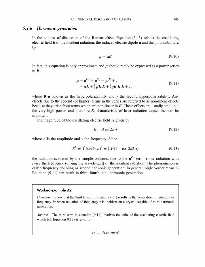
9.1.6 Harmonic generation
In the context of discussion of the Raman effect, Equation (5.43) relates the oscillating
electric field E of the incident radiation, the induced electric dipole mm and the polarizability aaby
mm ¼ aaE ð9:10Þ
In fact, this equation is only approximate and mm should really be expressed as a power series
in E
mm ¼ mmð1Þ þ mmð2Þ þ mmð3Þ þ : : :
¼ aaE þ 12bbE:E þ 1
6cE:E:E þ : : :
ð9:11Þ
where bb is known as the hyperpolarizability and c the second hyperpolarizability. Any
effects due to the second (or higher) terms in the series are referred to as non-linear effects
because they arise from terms which are non-linear in E. These effects are usually small but
the very high power, and therefore E, characteristic of laser radiation causes them to be
important.
The magnitude of the oscillating electric field is given by
E ¼ A sin 2pnt ð9:12Þ
where A is the amplitude and n the frequency. Since
E2 ¼ A2ðsin 2pntÞ2 ¼ 12A2ð1� cos 2p2ntÞ ð9:13Þ
the radiation scattered by the sample contains, due to the mmð2Þ term, some radiation with
twice the frequency (or half the wavelength) of the incident radiation. The phenomenon is
called frequency doubling or second harmonic generation. In general, higher-order terms in
Equation (9.11) can result in third, fourth, etc., harmonic generation.
Worked example 9.2
Question. Show that the third term in Equation (9.11) results in the generation of radiation of
frequency 3n when radiation of frequency n is incident on a crystal capable of third harmonic
generation.
Answer. The third term in equation (9.11) involves the cube of the oscillating electric field
which (cf. Equation 9.13) is given by
E3 ¼ A3ðsin 2pntÞ3
9.1 GENERAL DISCUSSION OF LASERS 345
But, in general, sin3 y ¼ 34sin y� 1
4sin 3y
; E3 ¼ A3 3
4sin 2pnt � 1
4sin 2p3nt
� �
Because the second term in the brackets contains 3n in the sine function, radiation at a
frequency which is three times that of the incident radiation is generated. This is referred to as
third harmonic generation. The first term in brackets indicates that some radiation of unchanged
frequency also results.
There are several pure crystalline materials which may be used for frequency doubling.
Examples are ADP, KDP and KD*P, mentioned in Section 9.1.4, potassium pentaborate
(KB5O8, KPB), b-barium borate (BaB2O4, BBO) and lithium niobate (Li3NbO4), each
material being suitable for incident radiation of only a limited wavelength range in the
visible region. The importance of these materials is that a laser operating in the visible
region, of which there are a relatively large number, can be made to operate in the near-
ultraviolet, where there are relatively few.
The efficiency of frequency doubling is quite low, often only a few per cent, but it may be
as high as 20 to 30 per cent.
9.2 Examples of lasers
9.2.1 The ruby and alexandrite lasers
After the ammonia maser, operating in the microwave region and constructed by Townes et
al. in 1954, the next major step forward was the ruby laser, operating in the red region of the
spectrum and demonstrated in 1960 by Maiman. This is a solid state laser employing a ruby
crystal consisting of aluminium oxide, Al2O3, containing 0.5 per cent by weight of Cr2O3,
giving it a pale pink colour.
The lasing constituent is the Cr3þ ion which is in such low concentration that it can be
regarded as a free ion. The ground configuration of Cr3þ (see Table 7.1) is KL3s23p63d3,
which gives rise to eight terms (see Table 7.2) of which 4F is, according to Hund’s rules (see
Section 7.1.2.3b), the lowest lying (ground) term. Of the others 2G is the lowest excited
term. Each Cr3þ ion is in a crystal field (see Section 7.3.1.4a) of approximately octahedral
symmetry. In the octahedral point group Oh, the4F ground term gives 4A2,
4T1 and 4T2states, and the 2G excited term gives 2A1,
2E, 2T1 and 2T2 states. Of these, 4A2 is the
ground state and 4T1,4T2,
2E and 2T2 are relatively low-lying excited states: all are shown in
Figure 9.6(a).
The 4T1 and 4T2 states are broadened as a result of slight variations in the crystal field.
The 2T2 and 2E states are sharper but the 2E state is split into two components, 29 cm71
apart, because of the slight distortion of the octahedral field. Population inversion and
346 9 LASERS AND LASER SPECTROSCOPY
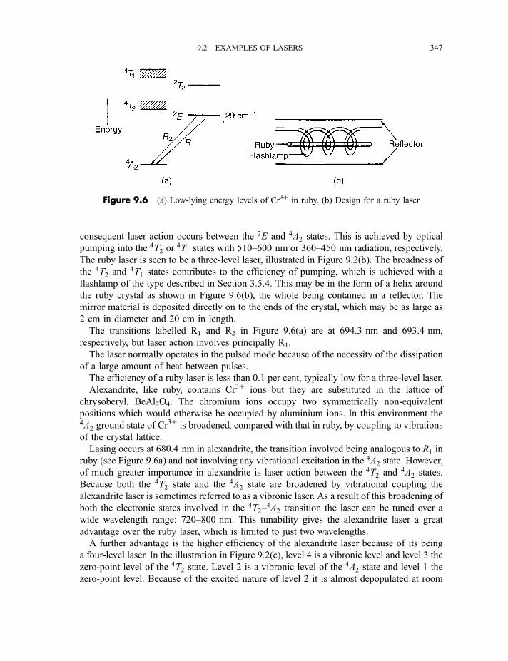
consequent laser action occurs between the 2E and 4A2 states. This is achieved by optical
pumping into the 4T2 or4T1 states with 510–600 nm or 360–450 nm radiation, respectively.
The ruby laser is seen to be a three-level laser, illustrated in Figure 9.2(b). The broadness of
the 4T2 and 4T1 states contributes to the efficiency of pumping, which is achieved with a
flashlamp of the type described in Section 3.5.4. This may be in the form of a helix around
the ruby crystal as shown in Figure 9.6(b), the whole being contained in a reflector. The
mirror material is deposited directly on to the ends of the crystal, which may be as large as
2 cm in diameter and 20 cm in length.
The transitions labelled R1 and R2 in Figure 9.6(a) are at 694.3 nm and 693.4 nm,
respectively, but laser action involves principally R1.
The laser normally operates in the pulsed mode because of the necessity of the dissipation
of a large amount of heat between pulses.
The efficiency of a ruby laser is less than 0.1 per cent, typically low for a three-level laser.
Alexandrite, like ruby, contains Cr3þ ions but they are substituted in the lattice of
chrysoberyl, BeAl2O4. The chromium ions occupy two symmetrically non-equivalent
positions which would otherwise be occupied by aluminium ions. In this environment the4A2 ground state of Cr
3þ is broadened, compared with that in ruby, by coupling to vibrations
of the crystal lattice.
Lasing occurs at 680.4 nm in alexandrite, the transition involved being analogous to R1 in
ruby (see Figure 9.6a) and not involving any vibrational excitation in the 4A2 state. However,
of much greater importance in alexandrite is laser action between the 4T2 and 4A2 states.
Because both the 4T2 state and the 4A2 state are broadened by vibrational coupling the
alexandrite laser is sometimes referred to as a vibronic laser. As a result of this broadening of
both the electronic states involved in the 4T2–4A2 transition the laser can be tuned over a
wide wavelength range: 720–800 nm. This tunability gives the alexandrite laser a great
advantage over the ruby laser, which is limited to just two wavelengths.
A further advantage is the higher efficiency of the alexandrite laser because of its being
a four-level laser. In the illustration in Figure 9.2(c), level 4 is a vibronic level and level 3 the
zero-point level of the 4T2 state. Level 2 is a vibronic level of the 4A2 state and level 1 the
zero-point level. Because of the excited nature of level 2 it is almost depopulated at room
Figure 9.6 (a) Low-lying energy levels of Cr3þ in ruby. (b) Design for a ruby laser
9.2 EXAMPLES OF LASERS 347
temperature so that a population inversion between levels 3 and 2 is relatively easy to
achieve. In fact, level 2 is a continuous band of vibronic levels covering a wide energy range,
resulting in the wide wavelength range over which the laser is tunable.
Pumping is with a flashlamp, as in the case of the ruby laser, and a pulse energy of the
order 1 J may be achieved. Frequency doubling (second harmonic generation) can provide
tunable radiation in the 360–400 nm region.
9.2.2 The titanium–sapphire laser
Despite the fact that the first laser to be produced (the ruby laser, Section 9.2.1) has the
remarkable property of having all its power concentrated into one or two wavelengths, a
property possessed by most lasers, it was soon realized that the inability to change these
wavelengths appreciably, that is to tune the laser, is a serious drawback which limits the
range of possible applications.
Historically, the first type of laser to be tunable over an appreciable wavelength range was
the dye laser, to be described in Section 9.2.10. The alexandrite laser (Section 9.2.1), a
tunable solid state laser, was first demonstrated in 1978 and then, in 1982, the titanium–
sapphire laser. This is also a solid state laser but tunable over a larger wavelength range,
670–1100 nm, than the alexandrite laser, which has a range of 720–800 nm.
The lasing medium in the titanium–sapphire laser is crystalline sapphire (Al2O3) with
about 0.1 per cent by weight of Ti2O3. The titanium is present as Ti3þ and it is between
energy levels of this ion that lasing occurs.
The ground configuration of Ti3þ (see Table 7.1) is KL3s23p63d1. The crystal field
experienced by the ion splits the 3d orbital into a triply degenerate lower-energy t2 orbital
and a doubly degenerate higher-energy e orbital (see Figure 7.38). If the electron is in the
lower orbital a 2T2 ground state results and, if it is in the upper orbital, a 2E excited state
results. These states are about 19 000 cm71 apart but each is split into further components
and is also coupled to the vibrations of the crystal lattice. In a similar way to that in
alexandrite (Section 9.2.1) population inversion can be created between these two sets of
levels resulting in a four-level vibronic laser with a tunable range of 670–1100 nm.
A further advantage, compared with the alexandrite laser, apart from a wider tuning range,
is that it can operate in the CW as well as in the pulsed mode. In the CW mode the Ti3þ–sapphire laser may be pumped by a CW argon ion laser (see Section 9.2.6) and is capable of
producing an output power of 5 W. In the pulsed mode pumping is usually achieved by a
pulsed Nd3þ : YAG laser (see Section 9.2.3) and a pulse energy of 100 mJ may be achieved.
In 1991 a remarkable discovery was made, accidentally, with a Ti3þ–sapphire laser
pumped with an Arþ laser. Whereas we would expect this to result in CW laser action, when
a sharp jolt was given to the table supporting the laser, mode locking (Section 9.1.5)
occurred. This is known as self-locking of modes, and we shall not discuss further the
reasons for this and how it can be controlled. One very important property of the resulting
pulses is that they are very short. Pulse widths of a few tens of femtoseconds can be produced
routinely and with high pulse-to-pulse stability. Further modification to the laser can
348 9 LASERS AND LASER SPECTROSCOPY
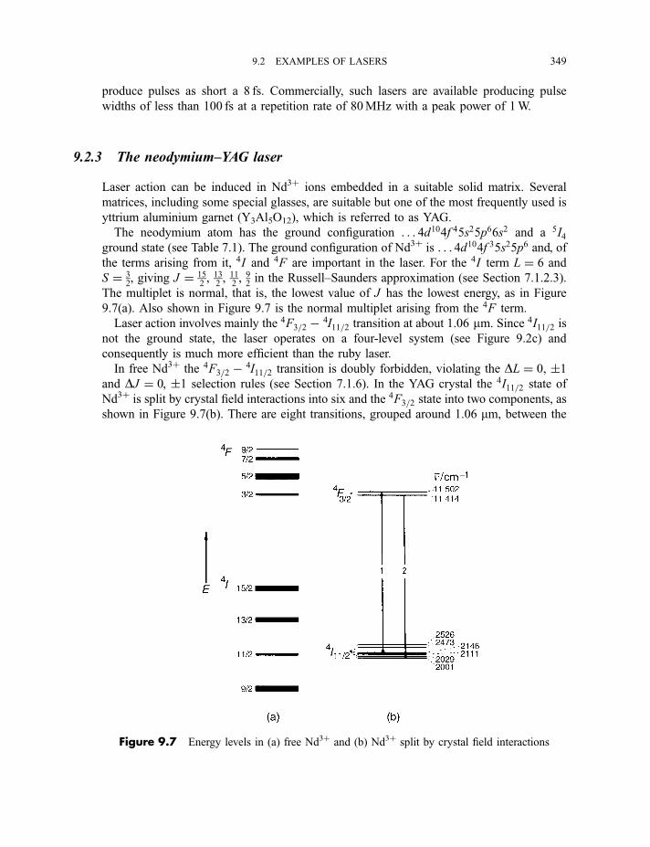
produce pulses as short a 8 fs. Commercially, such lasers are available producing pulse
widths of less than 100 fs at a repetition rate of 80MHz with a peak power of 1W.
9.2.3 The neodymium–YAG laser
Laser action can be induced in Nd3þ ions embedded in a suitable solid matrix. Several
matrices, including some special glasses, are suitable but one of the most frequently used is
yttrium aluminium garnet (Y3Al5O12), which is referred to as YAG.
The neodymium atom has the ground configuration . . . 4d104f 45s25p66s2 and a 5I4ground state (see Table 7.1). The ground configuration of Nd3þ is . . . 4d104f 35s25p6 and, ofthe terms arising from it, 4I and 4F are important in the laser. For the 4I term L ¼ 6 and
S ¼ 32, giving J ¼ 15
2, 13
2, 11
2, 92in the Russell–Saunders approximation (see Section 7.1.2.3).
The multiplet is normal, that is, the lowest value of J has the lowest energy, as in Figure
9.7(a). Also shown in Figure 9.7 is the normal multiplet arising from the 4F term.
Laser action involves mainly the 4F3=2 � 4I11=2 transition at about 1.06 mm. Since 4I11=2 is
not the ground state, the laser operates on a four-level system (see Figure 9.2c) and
consequently is much more efficient than the ruby laser.
In free Nd3þ the 4F3=2 � 4I11=2 transition is doubly forbidden, violating the DL ¼ 0, �1and DJ ¼ 0, �1 selection rules (see Section 7.1.6). In the YAG crystal the 4I11=2 state of
Nd3þ is split by crystal field interactions into six and the 4F3=2 state into two components, as
shown in Figure 9.7(b). There are eight transitions, grouped around 1.06 mm, between the
Figure 9.7 Energy levels in (a) free Nd3þ and (b) Nd3þ split by crystal field interactions
9.2 EXAMPLES OF LASERS 349
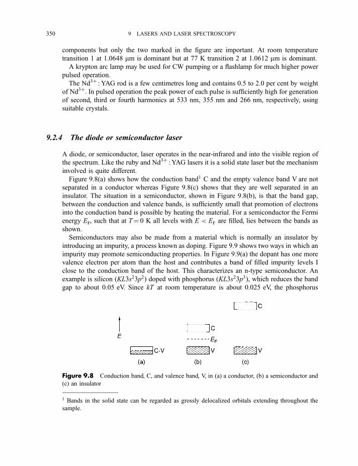
components but only the two marked in the figure are important. At room temperature
transition 1 at 1.0648 mm is dominant but at 77 K transition 2 at 1.0612 mm is dominant.
A krypton arc lamp may be used for CW pumping or a flashlamp for much higher power
pulsed operation.
The Nd3þ : YAG rod is a few centimetres long and contains 0.5 to 2.0 per cent by weight
of Nd3þ. In pulsed operation the peak power of each pulse is sufficiently high for generation
of second, third or fourth harmonics at 533 nm, 355 nm and 266 nm, respectively, using
suitable crystals.
9.2.4 The diode or semiconductor laser
A diode, or semiconductor, laser operates in the near-infrared and into the visible region of
the spectrum. Like the ruby and Nd3þ : YAG lasers it is a solid state laser but the mechanism
involved is quite different.
Figure 9.8(a) shows how the conduction band1 C and the empty valence band V are not
separated in a conductor whereas Figure 9.8(c) shows that they are well separated in an
insulator. The situation in a semiconductor, shown in Figure 9.8(b), is that the band gap,
between the conduction and valence bands, is sufficiently small that promotion of electrons
into the conduction band is possible by heating the material. For a semiconductor the Fermi
energy EF, such that at T¼ 0 K all levels with E < EF are filled, lies between the bands as
shown.
Semiconductors may also be made from a material which is normally an insulator by
introducing an impurity, a process known as doping. Figure 9.9 shows two ways in which an
impurity may promote semiconducting properties. In Figure 9.9(a) the dopant has one more
valence electron per atom than the host and contributes a band of filled impurity levels I
close to the conduction band of the host. This characterizes an n-type semiconductor. An
example is silicon ðKL3s23p2Þ doped with phosphorus ðKL3s23p3Þ, which reduces the band
gap to about 0.05 eV. Since kT at room temperature is about 0.025 eV, the phosphorus
1 Bands in the solid state can be regarded as grossly delocalized orbitals extending throughout the
sample.
Figure 9.8 Conduction band, C, and valence band, V, in (a) a conductor, (b) a semiconductor and
(c) an insulator
350 9 LASERS AND LASER SPECTROSCOPY
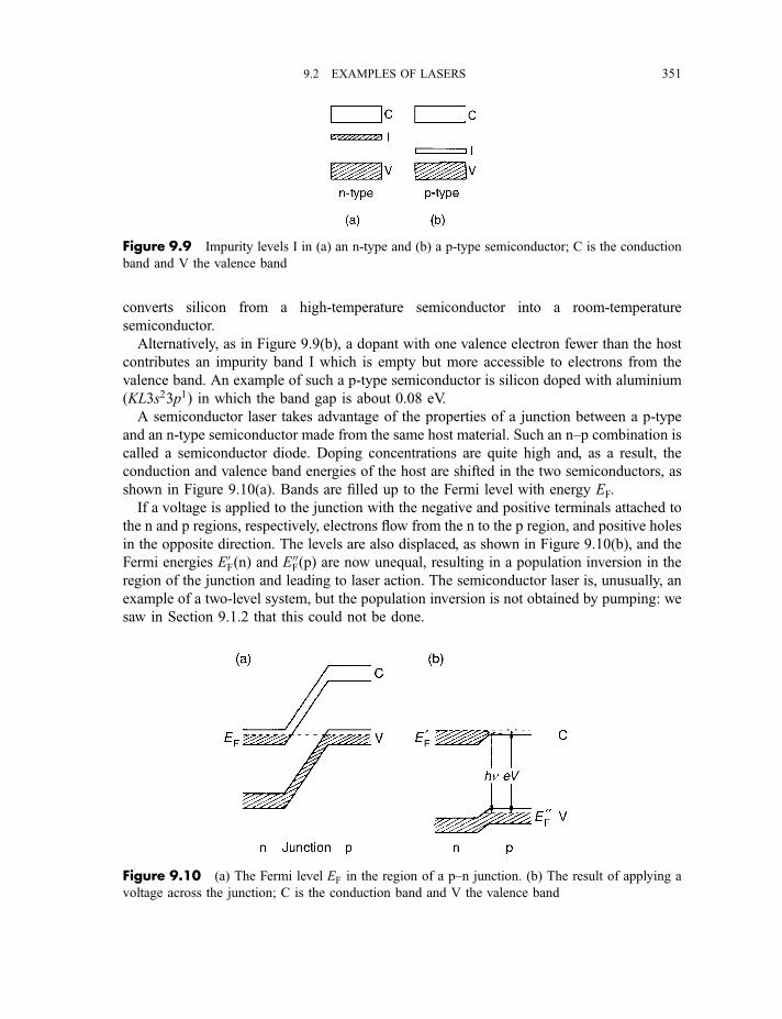
converts silicon from a high-temperature semiconductor into a room-temperature
semiconductor.
Alternatively, as in Figure 9.9(b), a dopant with one valence electron fewer than the host
contributes an impurity band I which is empty but more accessible to electrons from the
valence band. An example of such a p-type semiconductor is silicon doped with aluminium
ðKL3s23p1Þ in which the band gap is about 0.08 eV.
A semiconductor laser takes advantage of the properties of a junction between a p-type
and an n-type semiconductor made from the same host material. Such an n–p combination is
called a semiconductor diode. Doping concentrations are quite high and, as a result, the
conduction and valence band energies of the host are shifted in the two semiconductors, as
shown in Figure 9.10(a). Bands are filled up to the Fermi level with energy EF.
If a voltage is applied to the junction with the negative and positive terminals attached to
the n and p regions, respectively, electrons flow from the n to the p region, and positive holes
in the opposite direction. The levels are also displaced, as shown in Figure 9.10(b), and the
Fermi energies E0FðnÞ and E00FðpÞ are now unequal, resulting in a population inversion in the
region of the junction and leading to laser action. The semiconductor laser is, unusually, an
example of a two-level system, but the population inversion is not obtained by pumping: we
saw in Section 9.1.2 that this could not be done.
Figure 9.9 Impurity levels I in (a) an n-type and (b) a p-type semiconductor; C is the conduction
band and V the valence band
Figure 9.10 (a) The Fermi level EF in the region of a p–n junction. (b) The result of applying a
voltage across the junction; C is the conduction band and V the valence band
9.2 EXAMPLES OF LASERS 351
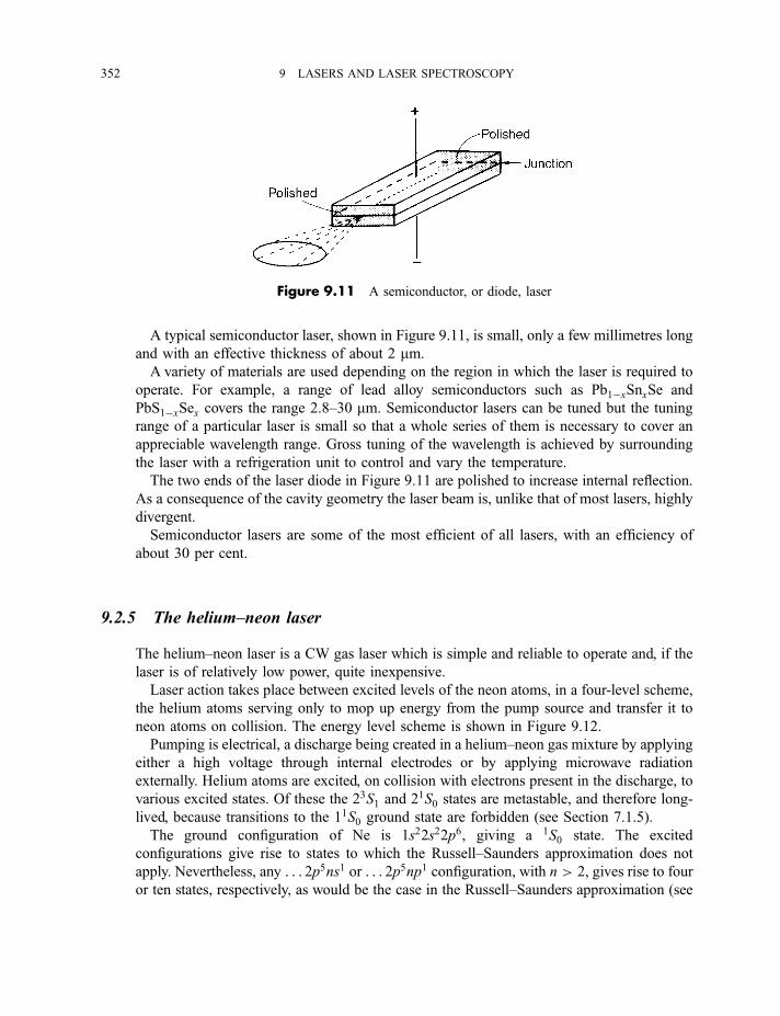
A typical semiconductor laser, shown in Figure 9.11, is small, only a few millimetres long
and with an effective thickness of about 2 mm.
A variety of materials are used depending on the region in which the laser is required to
operate. For example, a range of lead alloy semiconductors such as Pb1�xSnxSe and
PbS1�xSex covers the range 2.8–30 mm. Semiconductor lasers can be tuned but the tuning
range of a particular laser is small so that a whole series of them is necessary to cover an
appreciable wavelength range. Gross tuning of the wavelength is achieved by surrounding
the laser with a refrigeration unit to control and vary the temperature.
The two ends of the laser diode in Figure 9.11 are polished to increase internal reflection.
As a consequence of the cavity geometry the laser beam is, unlike that of most lasers, highly
divergent.
Semiconductor lasers are some of the most efficient of all lasers, with an efficiency of
about 30 per cent.
9.2.5 The helium–neon laser
The helium–neon laser is a CW gas laser which is simple and reliable to operate and, if the
laser is of relatively low power, quite inexpensive.
Laser action takes place between excited levels of the neon atoms, in a four-level scheme,
the helium atoms serving only to mop up energy from the pump source and transfer it to
neon atoms on collision. The energy level scheme is shown in Figure 9.12.
Pumping is electrical, a discharge being created in a helium–neon gas mixture by applying
either a high voltage through internal electrodes or by applying microwave radiation
externally. Helium atoms are excited, on collision with electrons present in the discharge, to
various excited states. Of these the 23S1 and 21S0 states are metastable, and therefore long-
lived, because transitions to the 11S0 ground state are forbidden (see Section 7.1.5).
The ground configuration of Ne is 1s22s22p6, giving a 1S0 state. The excited
configurations give rise to states to which the Russell–Saunders approximation does not
apply. Nevertheless, any . . . 2p5ns1 or . . . 2p5np1 configuration, with n > 2, gives rise to four
or ten states, respectively, as would be the case in the Russell–Saunders approximation (see
Figure 9.11 A semiconductor, or diode, laser
352 9 LASERS AND LASER SPECTROSCOPY
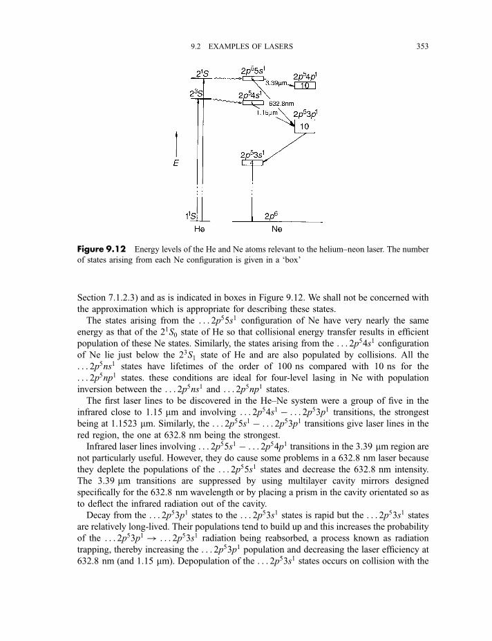
Section 7.1.2.3) and as is indicated in boxes in Figure 9.12. We shall not be concerned with
the approximation which is appropriate for describing these states.
The states arising from the . . . 2p55s1 configuration of Ne have very nearly the same
energy as that of the 21S0 state of He so that collisional energy transfer results in efficient
population of these Ne states. Similarly, the states arising from the . . . 2p54s1 configurationof Ne lie just below the 23S1 state of He and are also populated by collisions. All the
. . . 2p5ns1 states have lifetimes of the order of 100 ns compared with 10 ns for the
. . . 2p5np1 states. these conditions are ideal for four-level lasing in Ne with population
inversion between the . . . 2p5ns1 and . . . 2p5np1 states.
The first laser lines to be discovered in the He–Ne system were a group of five in the
infrared close to 1.15 mm and involving . . . 2p54s1 � . . . 2p53p1 transitions, the strongest
being at 1.1523 mm. Similarly, the . . . 2p55s1 � . . . 2p53p1 transitions give laser lines in the
red region, the one at 632.8 nm being the strongest.
Infrared laser lines involving . . . 2p55s1 � . . . 2p54p1 transitions in the 3.39 mm region are
not particularly useful. However, they do cause some problems in a 632.8 nm laser because
they deplete the populations of the . . . 2p55s1 states and decrease the 632.8 nm intensity.
The 3.39 mm transitions are suppressed by using multilayer cavity mirrors designed
specifically for the 632.8 nm wavelength or by placing a prism in the cavity orientated so as
to deflect the infrared radiation out of the cavity.
Decay from the . . . 2p53p1 states to the . . . 2p53s1 states is rapid but the . . . 2p53s1 statesare relatively long-lived. Their populations tend to build up and this increases the probability
of the . . . 2p53p1! . . . 2p53s1 radiation being reabsorbed, a process known as radiation
trapping, thereby increasing the . . . 2p53p1 population and decreasing the laser efficiency at
632.8 nm (and 1.15 mm). Depopulation of the . . . 2p53s1 states occurs on collision with the
Figure 9.12 Energy levels of the He and Ne atoms relevant to the helium–neon laser. The number
of states arising from each Ne configuration is given in a ‘box’
9.2 EXAMPLES OF LASERS 353
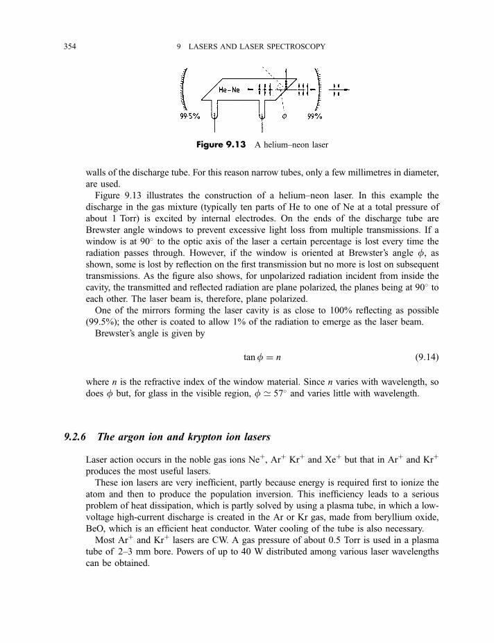
walls of the discharge tube. For this reason narrow tubes, only a few millimetres in diameter,
are used.
Figure 9.13 illustrates the construction of a helium–neon laser. In this example the
discharge in the gas mixture (typically ten parts of He to one of Ne at a total pressure of
about 1 Torr) is excited by internal electrodes. On the ends of the discharge tube are
Brewster angle windows to prevent excessive light loss from multiple transmissions. If a
window is at 90� to the optic axis of the laser a certain percentage is lost every time the
radiation passes through. However, if the window is oriented at Brewster’s angle f, asshown, some is lost by reflection on the first transmission but no more is lost on subsequent
transmissions. As the figure also shows, for unpolarized radiation incident from inside the
cavity, the transmitted and reflected radiation are plane polarized, the planes being at 90� toeach other. The laser beam is, therefore, plane polarized.
One of the mirrors forming the laser cavity is as close to 100% reflecting as possible
(99.5%); the other is coated to allow 1% of the radiation to emerge as the laser beam.
Brewster’s angle is given by
tanf ¼ n ð9:14Þ
where n is the refractive index of the window material. Since n varies with wavelength, so
does f but, for glass in the visible region, f ’ 57� and varies little with wavelength.
9.2.6 The argon ion and krypton ion lasers
Laser action occurs in the noble gas ions Neþ, Arþ Krþ and Xeþ but that in Arþ and Krþ
produces the most useful lasers.
These ion lasers are very inefficient, partly because energy is required first to ionize the
atom and then to produce the population inversion. This inefficiency leads to a serious
problem of heat dissipation, which is partly solved by using a plasma tube, in which a low-
voltage high-current discharge is created in the Ar or Kr gas, made from beryllium oxide,
BeO, which is an efficient heat conductor. Water cooling of the tube is also necessary.
Most Arþ and Krþ lasers are CW. A gas pressure of about 0.5 Torr is used in a plasma
tube of 2–3 mm bore. Powers of up to 40 W distributed among various laser wavelengths
can be obtained.
Figure 9.13 A helium–neon laser
354 9 LASERS AND LASER SPECTROSCOPY
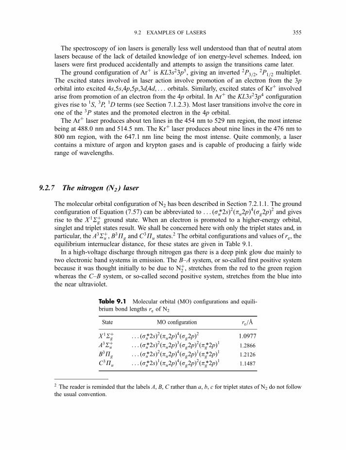
The spectroscopy of ion lasers is generally less well understood than that of neutral atom
lasers because of the lack of detailed knowledge of ion energy-level schemes. Indeed, ion
lasers were first produced accidentally and attempts to assign the transitions came later.
The ground configuration of Arþ is KL3s23p5, giving an inverted 2P3=2,2P1=2 multiplet.
The excited states involved in laser action involve promotion of an electron from the 3p
orbital into excited 4s,5s,4p,5p,3d,4d, . . . orbitals. Similarly, excited states of Krþ involved
arise from promotion of an electron from the 4p orbital. In Arþ the KL3s23p4 configuration
gives rise to 1S, 3P, 1D terms (see Section 7.1.2.3). Most laser transitions involve the core in
one of the 3P states and the promoted electron in the 4p orbital.
The Arþ laser produces about ten lines in the 454 nm to 529 nm region, the most intense
being at 488.0 nm and 514.5 nm. The Krþ laser produces about nine lines in the 476 nm to
800 nm region, with the 647.1 nm line being the most intense. Quite commonly, a laser
contains a mixture of argon and krypton gases and is capable of producing a fairly wide
range of wavelengths.
9.2.7 The nitrogen (N2 ) laser
The molecular orbital configuration of N2 has been described in Section 7.2.1.1. The ground
configuration of Equation (7.57) can be abbreviated to . . . ðsu*2sÞ2ðpu2pÞ4ðsg2pÞ2 and gives
rise to the X 1Sþg ground state. When an electron is promoted to a higher-energy orbital,
singlet and triplet states result. We shall be concerned here with only the triplet states and, in
particular, the A3Sþu , B3Pg and C3Pu states.
2 The orbital configurations and values of re, the
equilibrium internuclear distance, for these states are given in Table 9.1.
In a high-voltage discharge through nitrogen gas there is a deep pink glow due mainly to
two electronic band systems in emission. The B–A system, or so-called first positive system
because it was thought initially to be due to Nþ2 , stretches from the red to the green region
whereas the C–B system, or so-called second positive system, stretches from the blue into
the near ultraviolet.
Table 9.1 Molecular orbital (MO) configurations and equili-
brium bond lengths re of N2
State MO configuration re=A
X 1Sþg . . . ðsu*2sÞ2ðpu2pÞ4ðsg2pÞ2 1.0977
A3Sþu . . . ðsu*2sÞ2ðpu2pÞ3ðsg2pÞ2ðpg*2pÞ1 1.2866
B3Pg . . . ðsu*2sÞ2ðpu2pÞ4ðsg2pÞ1ðpg*2pÞ1 1.2126
C3Pu . . . ðsu*2sÞ1ðpu2pÞ4ðsg2pÞ2ðpg*2pÞ1 1.1487
2 The reader is reminded that the labels A, B, C rather than a, b, c for triplet states of N2 do not follow
the usual convention.
9.2 EXAMPLES OF LASERS 355
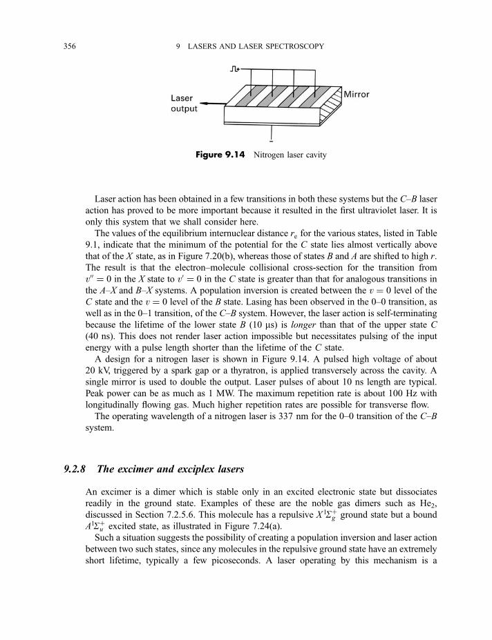
Laser action has been obtained in a few transitions in both these systems but the C–B laser
action has proved to be more important because it resulted in the first ultraviolet laser. It is
only this system that we shall consider here.
The values of the equilibrium internuclear distance re for the various states, listed in Table
9.1, indicate that the minimum of the potential for the C state lies almost vertically above
that of the X state, as in Figure 7.20(b), whereas those of states B and A are shifted to high r.
The result is that the electron–molecule collisional cross-section for the transition from
v00 ¼ 0 in the X state to v0 ¼ 0 in the C state is greater than that for analogous transitions in
the A–X and B–X systems. A population inversion is created between the v ¼ 0 level of the
C state and the v ¼ 0 level of the B state. Lasing has been observed in the 0–0 transition, as
well as in the 0–1 transition, of the C–B system. However, the laser action is self-terminating
because the lifetime of the lower state B (10 ms) is longer than that of the upper state C
(40 ns). This does not render laser action impossible but necessitates pulsing of the input
energy with a pulse length shorter than the lifetime of the C state.
A design for a nitrogen laser is shown in Figure 9.14. A pulsed high voltage of about
20 kV, triggered by a spark gap or a thyratron, is applied transversely across the cavity. A
single mirror is used to double the output. Laser pulses of about 10 ns length are typical.
Peak power can be as much as 1 MW. The maximum repetition rate is about 100 Hz with
longitudinally flowing gas. Much higher repetition rates are possible for transverse flow.
The operating wavelength of a nitrogen laser is 337 nm for the 0–0 transition of the C–B
system.
9.2.8 The excimer and exciplex lasers
An excimer is a dimer which is stable only in an excited electronic state but dissociates
readily in the ground state. Examples of these are the noble gas dimers such as He2,
discussed in Section 7.2.5.6. This molecule has a repulsive X 1Sþg ground state but a bound
A1Sþu excited state, as illustrated in Figure 7.24(a).
Such a situation suggests the possibility of creating a population inversion and laser action
between two such states, since any molecules in the repulsive ground state have an extremely
short lifetime, typically a few picoseconds. A laser operating by this mechanism is a
Figure 9.14 Nitrogen laser cavity
356 9 LASERS AND LASER SPECTROSCOPY
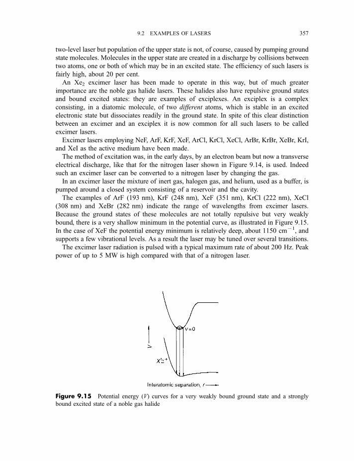
two-level laser but population of the upper state is not, of course, caused by pumping ground
state molecules. Molecules in the upper state are created in a discharge by collisions between
two atoms, one or both of which may be in an excited state. The efficiency of such lasers is
fairly high, about 20 per cent.
An Xe2 excimer laser has been made to operate in this way, but of much greater
importance are the noble gas halide lasers. These halides also have repulsive ground states
and bound excited states: they are examples of exciplexes. An exciplex is a complex
consisting, in a diatomic molecule, of two different atoms, which is stable in an excited
electronic state but dissociates readily in the ground state. In spite of this clear distinction
between an excimer and an exciplex it is now common for all such lasers to be called
excimer lasers.
Excimer lasers employing NeF, ArF, KrF, XeF, ArCl, KrCl, XeCl, ArBr, KrBr, XeBr, KrI,
and XeI as the active medium have been made.
The method of excitation was, in the early days, by an electron beam but now a transverse
electrical discharge, like that for the nitrogen laser shown in Figure 9.14, is used. Indeed
such an excimer laser can be converted to a nitrogen laser by changing the gas.
In an excimer laser the mixture of inert gas, halogen gas, and helium, used as a buffer, is
pumped around a closed system consisting of a reservoir and the cavity.
The examples of ArF (193 nm), KrF (248 nm), XeF (351 nm), KrCl (222 nm), XeCl
(308 nm) and XeBr (282 nm) indicate the range of wavelengths from excimer lasers.
Because the ground states of these molecules are not totally repulsive but very weakly
bound, there is a very shallow minimum in the potential curve, as illustrated in Figure 9.15.
In the case of XeF the potential energy minimum is relatively deep, about 1150 cm71, and
supports a few vibrational levels. As a result the laser may be tuned over several transitions.
The excimer laser radiation is pulsed with a typical maximum rate of about 200 Hz. Peak
power of up to 5 MW is high compared with that of a nitrogen laser.
Figure 9.15 Potential energy (V) curves for a very weakly bound ground state and a strongly
bound excited state of a noble gas halide
9.2 EXAMPLES OF LASERS 357
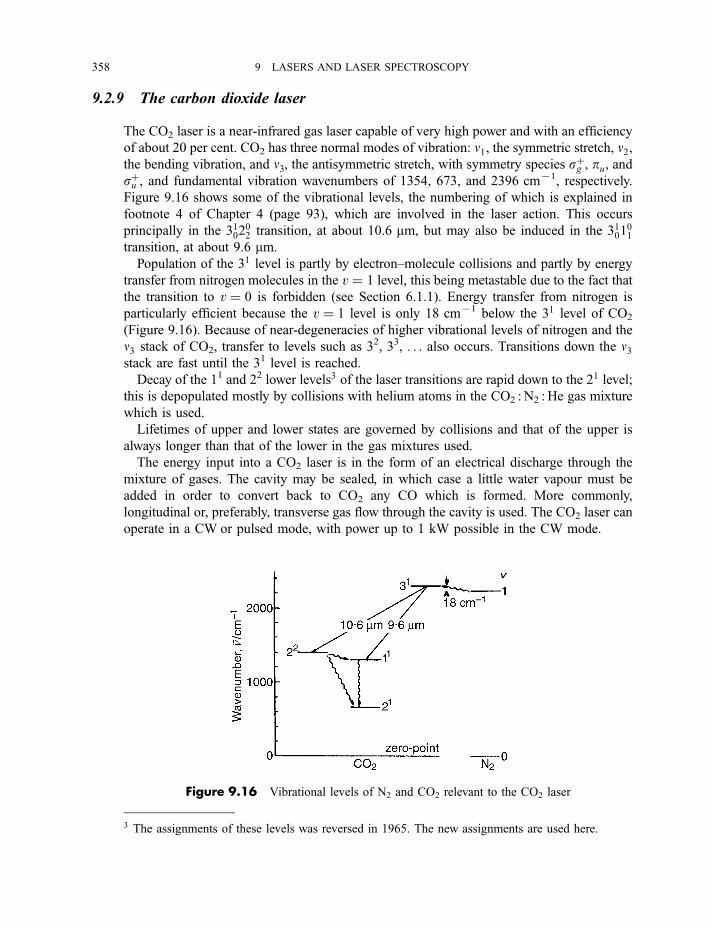
9.2.9 The carbon dioxide laser
The CO2 laser is a near-infrared gas laser capable of very high power and with an efficiency
of about 20 per cent. CO2 has three normal modes of vibration: n1, the symmetric stretch, n2,the bending vibration, and n3, the antisymmetric stretch, with symmetry species sþg , pu, andsþu , and fundamental vibration wavenumbers of 1354, 673, and 2396 cm71, respectively.
Figure 9.16 shows some of the vibrational levels, the numbering of which is explained in
footnote 4 of Chapter 4 (page 93), which are involved in the laser action. This occurs
principally in the 310202 transition, at about 10.6 mm, but may also be induced in the 3101
01
transition, at about 9.6 mm.
Population of the 31 level is partly by electron–molecule collisions and partly by energy
transfer from nitrogen molecules in the v ¼ 1 level, this being metastable due to the fact that
the transition to v ¼ 0 is forbidden (see Section 6.1.1). Energy transfer from nitrogen is
particularly efficient because the v ¼ 1 level is only 18 cm71 below the 31 level of CO2
(Figure 9.16). Because of near-degeneracies of higher vibrational levels of nitrogen and the
n3 stack of CO2, transfer to levels such as 32, 33, . . . also occurs. Transitions down the n3stack are fast until the 31 level is reached.
Decay of the 11 and 22 lower levels3 of the laser transitions are rapid down to the 21 level;
this is depopulated mostly by collisions with helium atoms in the CO2 : N2 : He gas mixture
which is used.
Lifetimes of upper and lower states are governed by collisions and that of the upper is
always longer than that of the lower in the gas mixtures used.
The energy input into a CO2 laser is in the form of an electrical discharge through the
mixture of gases. The cavity may be sealed, in which case a little water vapour must be
added in order to convert back to CO2 any CO which is formed. More commonly,
longitudinal or, preferably, transverse gas flow through the cavity is used. The CO2 laser can
operate in a CW or pulsed mode, with power up to 1 kW possible in the CW mode.
Figure 9.16 Vibrational levels of N2 and CO2 relevant to the CO2 laser
3 The assignments of these levels was reversed in 1965. The new assignments are used here.
358 9 LASERS AND LASER SPECTROSCOPY
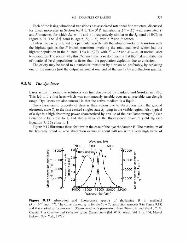
Each of the lasing vibrational transitions has associated rotational fine structure, discussed
for linear molecules in Section 6.2.4.1. The 310101 transition is Sþu � Sþg with associated P
and R branches, for which DJ ¼ �1 and þ1, respectively, similar to the 310 band of HCN in
Figure 6.25. The 310202 band is, again, Sþu � Sþg with a P and R branch.
Unless the cavity is tuned to a particular wavelength the vibration–rotation transition with
the highest gain is the P-branch transition involving the rotational level which has the
highest population in the 31 state. This is Pð22Þ, with J 00 ¼ 22 and J 0 ¼ 21, at normal laser
temperatures. The reason why this P-branch line is so dominant is that thermal redistribution
of rotational level populations is faster than the population depletion due to emission.
The cavity may be tuned to a particular transition by a prism or, preferably, by replacing
one of the mirrors (not the output mirror) at one end of the cavity by a diffraction grating.
9.2.10 The dye laser
Laser action in some dye solutions was first discovered by Lankard and Sorokin in 1966.
This led to the first laser which was continuously tunable over an appreciable wavelength
range. Dye lasers are also unusual in that the active medium is a liquid.
One characteristic property of dyes is their colour due to absorption from the ground
electronic state S0 to the first excited singlet state S1 lying in the visible region. Also typical
of a dye is a high absorbing power characterized by a value of the oscillator strength f (see
Equation 2.18) close to 1, and also a value of the fluorescence quantum yield FF (see
Equation 7.135) close to 1.
Figure 9.17 illustrates these features in the case of the dye rhodamine B. The maximum of
the typically broad S1 � S0 absorption occurs at about 548 nm with a very high value of
Figure 9.17 Absorption and fluorescence spectra of rhodamine B in methanol
(56 1075 mol l71). The curve marked eT is for the T2 � T1 absorption (process 8 in Figure 9.18)
and that marked eS for process 1. (Reproduced, with permission, from Dienes, A. and Shank, C. V.,
Chapter 4 in Creation and Detection of the Excited State (Ed. W. R. Ware), Vol. 2, p. 154, Marcel
Dekker, New York, 1972)
9.2 EXAMPLES OF LASERS 359
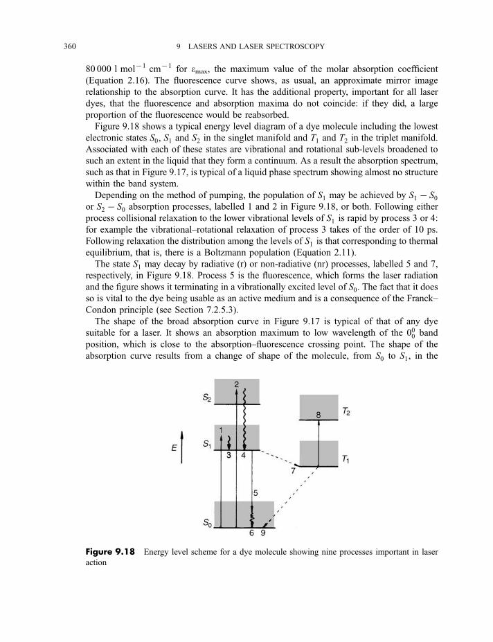
80 000 l mol71 cm71 for emax, the maximum value of the molar absorption coefficient
(Equation 2.16). The fluorescence curve shows, as usual, an approximate mirror image
relationship to the absorption curve. It has the additional property, important for all laser
dyes, that the fluorescence and absorption maxima do not coincide: if they did, a large
proportion of the fluorescence would be reabsorbed.
Figure 9.18 shows a typical energy level diagram of a dye molecule including the lowest
electronic states S0, S1 and S2 in the singlet manifold and T1 and T2 in the triplet manifold.
Associated with each of these states are vibrational and rotational sub-levels broadened to
such an extent in the liquid that they form a continuum. As a result the absorption spectrum,
such as that in Figure 9.17, is typical of a liquid phase spectrum showing almost no structure
within the band system.
Depending on the method of pumping, the population of S1 may be achieved by S1 � S0or S2 � S0 absorption processes, labelled 1 and 2 in Figure 9.18, or both. Following either
process collisional relaxation to the lower vibrational levels of S1 is rapid by process 3 or 4:
for example the vibrational–rotational relaxation of process 3 takes of the order of 10 ps.
Following relaxation the distribution among the levels of S1 is that corresponding to thermal
equilibrium, that is, there is a Boltzmann population (Equation 2.11).
The state S1 may decay by radiative (r) or non-radiative (nr) processes, labelled 5 and 7,
respectively, in Figure 9.18. Process 5 is the fluorescence, which forms the laser radiation
and the figure shows it terminating in a vibrationally excited level of S0. The fact that it does
so is vital to the dye being usable as an active medium and is a consequence of the Franck–
Condon principle (see Section 7.2.5.3).
The shape of the broad absorption curve in Figure 9.17 is typical of that of any dye
suitable for a laser. It shows an absorption maximum to low wavelength of the 000 band
position, which is close to the absorption–fluorescence crossing point. The shape of the
absorption curve results from a change of shape of the molecule, from S0 to S1, in the
Figure 9.18 Energy level scheme for a dye molecule showing nine processes important in laser
action
360 9 LASERS AND LASER SPECTROSCOPY
direction of one or more normal coordinates, so that the most probable transition in
absorption is to a vibrationally excited level of S1. Similarly, in emission from the zero-point
level of S1, the most probable transition is to a vibrationally excited level of S0. The
fluorescence lifetime tr for spontaneous emission from S1 is typically of the order of 1 ns
whereas the relaxation process 6, like process 3, takes only about 10 ps. The result is that,
following processes 1 and 3, there is a population inversion between the zero-point level of
S1 and vibrationally excited levels of S0 to which emission may occur, provided that these
levels are of sufficiently high energy to have negligible thermal population.
The population of S1 may also be reduced by absorption of the fluorescence taking the
molecule from S1 into S2, if the wavelengths of the two processes correspond, as well as by
non-radiative transitions to either S0 (internal conversion) or T1 (intersystem crossing), as
discussed in Section 7.3.6. In dye molecules it is the S1 � T1 process, labelled 7 in Figure
9.18, which is the most important. This is a spin-forbidden process with a lifetime tnr of theorder of 100 ns. The lifetime t of the state S1 is related to tnr and the radiative lifetime tr by
1
t¼ 1
trþ 1
tnrð9:15Þ
Since tr is of the order of 1 ns, fluorescence is the dominant decay process for S1.
The lifetime tT of the state T1 is long because the T1 � S0 transition, process 9 in Figure
9.18, is spin-forbidden. Depending on the molecule and on the conditions, particularly the
amount of dissolved oxygen, it may be anywhere in the range 100 ns to 1 ms. If tT > tnr theresult is that the concentration of molecules in T1 can build up to a high level. It happens in
many dye molecules that the intense, spin-allowed, T2 � T1 absorption, process 8 in Figure
9.18, overlaps with, and therefore can be excited by, the S1 � S0 emission, thereby
decreasing the efficiency of the laser considerably. Figure 9.17 shows how important this
process is in rhodamine B.
In order to prevent this occurring a pulsed method of pumping is used with a repetition
rate low enough to allow time for T1 � S0 relaxation. For CW operation either tT must be
sufficiently short or another dye has to be used for which T2 � T1 absorption does not
overlap with the fluorescence.
There are many dyes available, each of which can be used over a 20–30 nm range and
which, together, cover a wavelength range from about 365 nm in the ultraviolet to about
930 nm in the near-infrared. Dye concentrations are low, typically in the range 1072
mol l71 to 1074 mol l71.
Taking into account the possibility of frequency doubling (Section 9.1.6) dye lasers can
provide tunable radiation throughout the range 220–930 nm but with varying levels of
intensity and degrees of difficulty. The tunability and the extensive wavelength range make
dye lasers probably the most generally useful of all visible or ultraviolet lasers.
A pulsed dye laser may be pumped with a flashlamp surrounding the cell through which
the dye is flowing. With this method of excitation pulses from the dye laser about 1 ms longand with an energy of the order of 100 mJ can be obtained. Repetition rates are typically
low – up to about 30 Hz.
9.2 EXAMPLES OF LASERS 361
More commonly a pulsed dye laser is pumped with a nitrogen, excimer, or Nd3þ : YAGlaser. Both the nitrogen laser, operating at 337 nm, and a xenon fluoride excimer laser,
operating at 351 nm, excite the dye initially into a singlet excited state higher in energy than
S1. The Nd3þ : YAG laser is either frequency doubled to operate at 532 nm or frequency
tripled to operate at 355 nm depending on the dye that is being pumped. However, because
of the low efficiency of frequency tripling, it is more usual to mix the frequency-doubled dye
radiation, of wavelength lD, with the Nd3þ : YAG laser fundamental, of wavelength lF(1.0648 mm), in a non-linear crystal such as KDP (Section 9.1.6) to give a wavelength lwhere
1
l¼ 1
lDþ 1
lFð9:15aÞ
Pulse rates of about 50 Hz are typical.
CW dye lasers are usually pumped with an argon ion laser, up to about 1 Wof continuous
dye laser power being produced, compared with about 1 MW peak power which may be
produced in a pulsed dye laser.
In both CWand pulsed lasers the dye solution must be kept moving to prevent overheating
and decomposition. In a pulsed laser the dye is continuously flowed through the containing
cell. Alternatively, magnetic stirring may be adequate for low repetition rates and relatively
low power. In a CW laser the dye solution is usually in the form of a jet flowing rapidly
across the laser cavity.
9.2.11 Laser materials in general
In choosing the examples of lasers discussed in Sections 9.2.1 to 9.2.10 many have been left
out. These include the CO, H2O, HCN, colour centre, and chemical lasers, all operating in
the infrared region, and the green copper vapour laser. The examples that we have looked at
in some detail serve to show how disparate and arbitrary the materials seem to be. For
example, the fact that Ne atoms lase in a helium–neon laser does not mean that Ar, Kr and
Xe will lase also – they do not. Nor is it the case that because CO2 lases, the chemically
similar CS2 will lase also.
The potential for laser activity is not anything we can demand of any atom or molecule.
We should regard it as accidental that among the extremely complex sets of energy levels
associated with a few atoms or molecules there happens to be one (or more) pairs between
which it is possible to produce a population inversion and thereby create a laser.
9.3 Uses of lasers in spectroscopy
From 1960 onwards, the increasing availability of intense, monochromatic laser sources
provided a tremendous impetus to a wide range of spectroscopic investigations. The most
immediately obvious application of early, essentially non-tunable, lasers was to all types of
Raman spectroscopy in the gas, liquid or solid phase. The experimental techniques,
362 9 LASERS AND LASER SPECTROSCOPY
employing laser radiation, were described in Section 5.3.1. Examples of the quality of
spectra which can be obtained in the gas phase are to be found in Figure 5.17, which shows
the pure rotational Raman spectrum of 15N2, and Figure 6.9 which shows the vibration–
rotation Raman spectrum of the v¼ 1–0 transition in CO. Both of these spectra were
obtained with an argon ion laser.
Laser radiation is very much more intense, and the line width much smaller, than that
from, for example, a mercury arc, which was commonly used as a Raman source before 1960.
As a result, weaker Raman scattering can now be observed and higher resolution is obtainable.
In addition to carrying out conventional Raman experiments with laser sources new kinds
of Raman experiments became possible using Q-switched, giant pulse lasers to investigate
effects which arise from the non-linear relationship between the induced electric dipole and
the oscillating electric field (Equation 9.11). These are grouped under the general heading of
non-linear Raman effects.
For branches of spectroscopy other than Raman spectroscopy most laser sources may
appear to have a great disadvantage, that of non-tunability. In regions of the spectrum,
particularly the infrared where tunable lasers are not readily available, ways have been
devised for tuning, that is, shifting, the atomic or molecular energy levels concerned until
the transition being studied moves into coincidence with the laser radiation. This may be
achieved by applying an electric field to the sample, and the technique is called laser Stark
spectroscopy. The corresponding technique using a magnetic field is that of laser magnetic
resonance (or laser Zeeman) spectroscopy.
A useful way of changing the wavelength of some lasers, for example the CO2 infrared
laser, is to use isotopically substituted material in which the wavelengths of laser transitions
are appreciably altered.
In regions of the spectrum where a tunable laser is available it may be possible to use it to
obtain an absorption spectrum in the same way as a tunable klystron or backward wave
oscillator is used in microwave or millimetre wave spectroscopy (see Section 3.4.1).
Absorbance (Equation 2.16) is measured as a function of frequency or wavenumber. This
technique can be used with a diode laser to produce an infrared absorption spectrum. When
electronic transitions are being studied, greater sensitivity is usually achieved by monitoring
secondary processes which follow, and are directly related to, the absorption which has
occurred. Such processes include fluorescence, dissociation, or predissociation, and,
following the absorption of one or more additional photons, ionization. The spectrum
resulting from monitoring these processes usually resembles the absorption spectrum very
closely.
It may be apparent to the reader at this stage that, when lasers are used as spectroscopic
sources, we can no longer think in terms of generally applicable experimental methods. A
wide variety of ingenious techniques have been devised using laser sources and it will be
possible to describe only a few of them here.
9.3.1 Hyper Raman spectroscopy
We have seen in Equation (9.11) how the dipole moment induced in a material by radiation
falling on it contains a small contribution which is proportional to the square of the
9.3 USES OF LASERS IN SPECTROSCOPY 363
oscillating electric field E of the radiation. This field can be sufficiently large, when using a
Q-switched laser focused on the sample, that hyper Raman scattering, involving the
hyperpolarizability bb introduced in Equation (9.11), is sufficiently intense to be detected.
Hyper Raman scattering is at a wavenumber 2~nn0 � ~nnHR, where ~nn0 is the wavenumber of the
exciting radiation and �~nnHR and þ~nnHR are the Stokes and anti-Stokes hyper Raman
displacements, respectively. The hyper Raman scattering is well separated from the Raman
scattering, which is centred on ~nn0, but is extremely weak, even with a Q-switched laser.
Scattering of wavenumber 2~nn0 is called hyper Rayleigh scattering, by analogy with
Raleigh scattering of wavenumber ~nn0 (see Section 5.3.2). However, whereas Rayleigh
scattering always occurs, hyper Rayleigh scattering occurs only if the scattering material
does not have a centre of inversion (see Section 4.1.3). Frequency doubled radiation,
discussed in Section 9.1.6, consists of hyper Rayleigh scattering from a pure crystal.
Consequently, one of the necessary properties of the crystals used, such as ADP and KDP, is
that the unit cell does not have a centre of inversion.
The selection rules for molecular vibrations involved in hyper Raman scattering are
summarized by
Gðcv0Þ � GðbijkÞ � Gðcv
00Þ ¼ A ðor � AÞ ð9:16Þ
analogous to Equations (6.64) and (6.65) for Raman scattering, where c0v and c00v are the
upper and lower state vibrational wave functions, respectively, i, j and k can be x, y or z, and
A is the totally symmetric species of the point group to which the molecule belongs. If, as is
usually the case, the lower vibrational state is the zero-point level Gðc00v Þ ¼ A and Equation
(9.16) becomes
Gðc0vÞ ¼ GðbijkÞ ð9:17Þ
The hyperpolarizability is a tensor with eighteen elements bijk . We shall not go further into
their symmetry properties but important results of Equation (9.17) include:
1. Vibrations allowed in the infrared are also allowed in the hyper Raman effect.
2. In a molecule with a centre of inversion all hyper Raman active vibrations are u
vibrations, antisymmetric to inversion.
3. Some vibrations which are both Raman and infrared inactive may be allowed in the hyper
Raman effect. Indeed, the occasional appearance of such vibrations in Raman spectra in a
condensed phase has sometimes been attributed to an effect involving the hyperpolariz-
ability.
Figure 9.19 shows the hyper Raman spectrum of gaseous ethane, C2H6, which belongs to
the D3d point group [see Figure 4.11(i) and Table A.28 in Appendix A]. Ethane has a centre
of inversion and therefore there is no hyper Rayleigh scattering at 2~nn0. In the hyper Raman
spectrum a1u, a2u and eu vibrations are allowed. None of these is allowed in the Raman
364 9 LASERS AND LASER SPECTROSCOPY
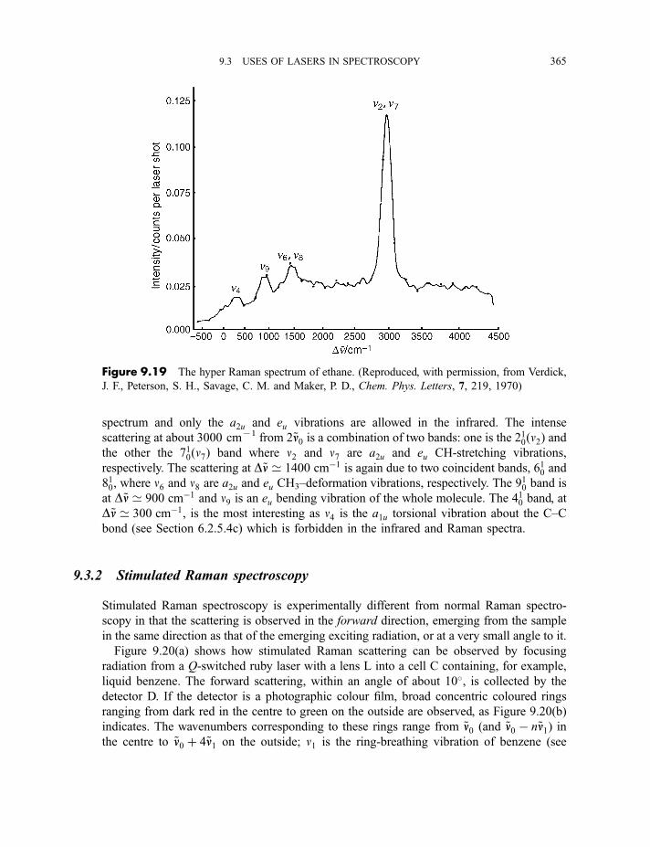
spectrum and only the a2u and eu vibrations are allowed in the infrared. The intense
scattering at about 3000 cm71 from 2~nn0 is a combination of two bands: one is the 210ðn2Þ andthe other the 710ðn7Þ band where n2 and n7 are a2u and eu CH-stretching vibrations,
respectively. The scattering at D~nn ’ 1400 cm�1 is again due to two coincident bands, 610 and
810, where n6 and n8 are a2u and eu CH3–deformation vibrations, respectively. The 910 band is
at D~nn ’ 900 cm�1 and n9 is an eu bending vibration of the whole molecule. The 410 band, at
D~nn ’ 300 cm�1, is the most interesting as n4 is the a1u torsional vibration about the C–C
bond (see Section 6.2.5.4c) which is forbidden in the infrared and Raman spectra.
9.3.2 Stimulated Raman spectroscopy
Stimulated Raman spectroscopy is experimentally different from normal Raman spectro-
scopy in that the scattering is observed in the forward direction, emerging from the sample
in the same direction as that of the emerging exciting radiation, or at a very small angle to it.
Figure 9.20(a) shows how stimulated Raman scattering can be observed by focusing
radiation from a Q-switched ruby laser with a lens L into a cell C containing, for example,
liquid benzene. The forward scattering, within an angle of about 10�, is collected by the
detector D. If the detector is a photographic colour film, broad concentric coloured rings
ranging from dark red in the centre to green on the outside are observed, as Figure 9.20(b)
indicates. The wavenumbers corresponding to these rings range from ~nn0 (and ~nn0 � n~nn1) inthe centre to ~nn0 þ 4~nn1 on the outside; n1 is the ring-breathing vibration of benzene (see
Figure 9.19 The hyper Raman spectrum of ethane. (Reproduced, with permission, from Verdick,
J. F., Peterson, S. H., Savage, C. M. and Maker, P. D., Chem. Phys. Letters, 7, 219, 1970)
9.3 USES OF LASERS IN SPECTROSCOPY 365
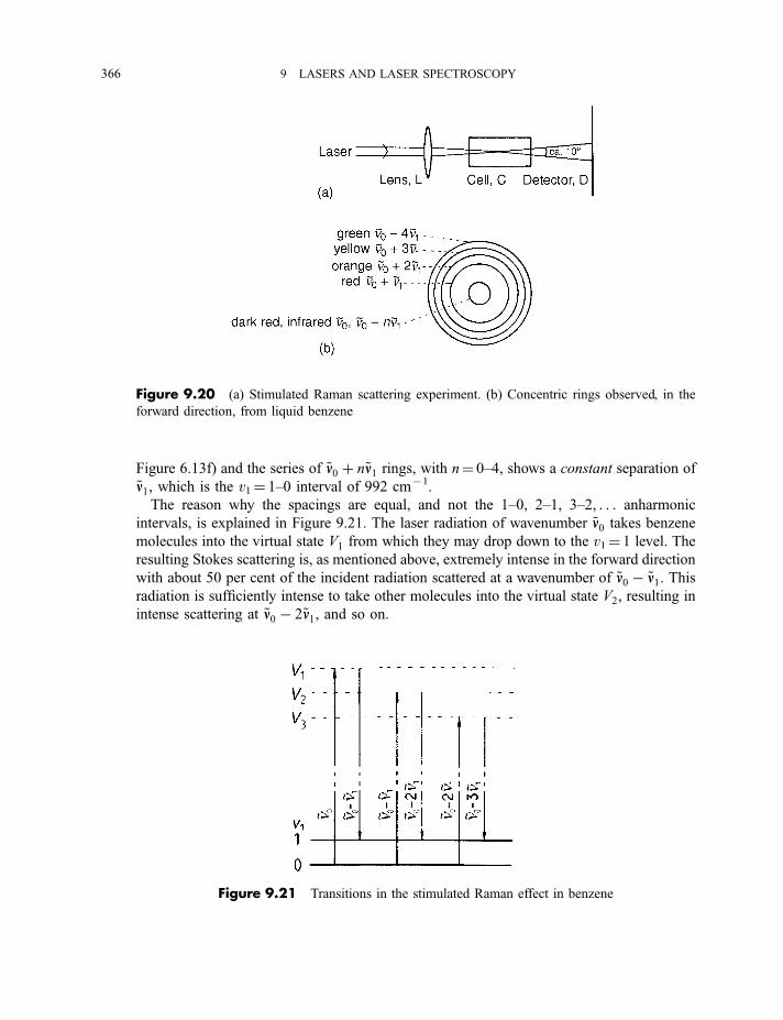
Figure 6.13f) and the series of ~nn0 þ n~nn1 rings, with n¼ 0–4, shows a constant separation of
~nn1, which is the v1¼ 1–0 interval of 992 cm71.
The reason why the spacings are equal, and not the 1–0, 2–1, 3–2, . . . anharmonic
intervals, is explained in Figure 9.21. The laser radiation of wavenumber ~nn0 takes benzene
molecules into the virtual state V1 from which they may drop down to the v1¼ 1 level. The
resulting Stokes scattering is, as mentioned above, extremely intense in the forward direction
with about 50 per cent of the incident radiation scattered at a wavenumber of ~nn0 � ~nn1. Thisradiation is sufficiently intense to take other molecules into the virtual state V2, resulting in
intense scattering at ~nn0 � 2~nn1, and so on.
Figure 9.20 (a) Stimulated Raman scattering experiment. (b) Concentric rings observed, in the
forward direction, from liquid benzene
Figure 9.21 Transitions in the stimulated Raman effect in benzene
366 9 LASERS AND LASER SPECTROSCOPY
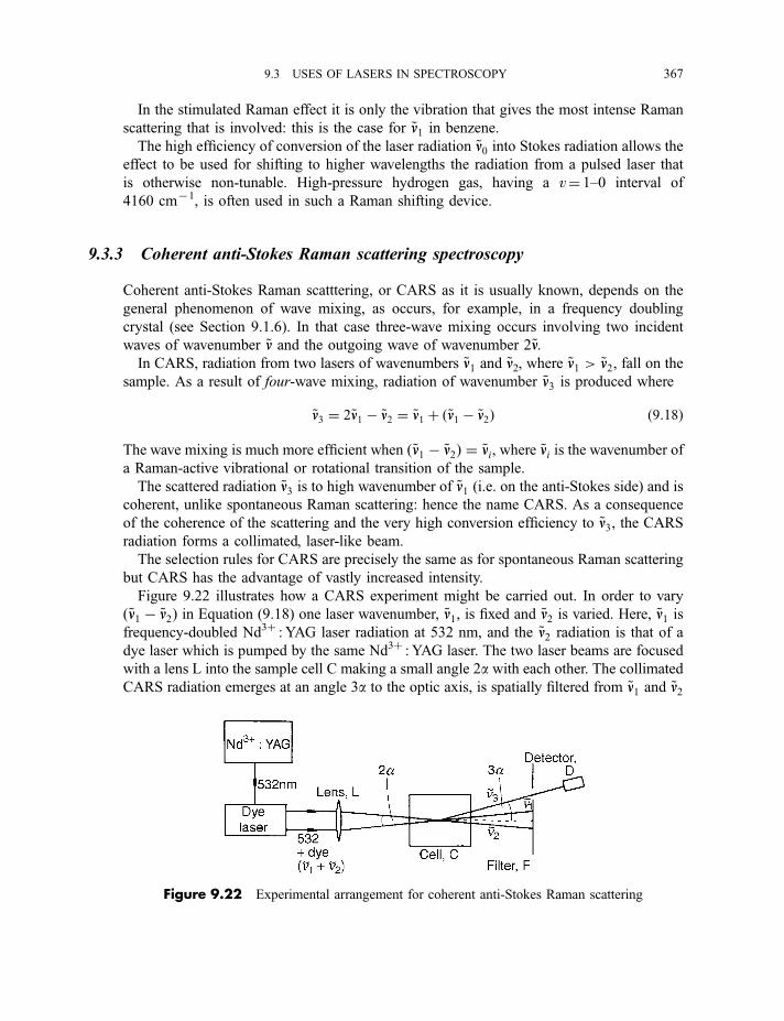
In the stimulated Raman effect it is only the vibration that gives the most intense Raman
scattering that is involved: this is the case for ~nn1 in benzene.
The high efficiency of conversion of the laser radiation ~nn0 into Stokes radiation allows the
effect to be used for shifting to higher wavelengths the radiation from a pulsed laser that
is otherwise non-tunable. High-pressure hydrogen gas, having a v¼ 1–0 interval of
4160 cm71, is often used in such a Raman shifting device.
9.3.3 Coherent anti-Stokes Raman scattering spectroscopy
Coherent anti-Stokes Raman scatttering, or CARS as it is usually known, depends on the
general phenomenon of wave mixing, as occurs, for example, in a frequency doubling
crystal (see Section 9.1.6). In that case three-wave mixing occurs involving two incident
waves of wavenumber ~nn and the outgoing wave of wavenumber 2~nn.In CARS, radiation from two lasers of wavenumbers ~nn1 and ~nn2, where ~nn1 > ~nn2, fall on the
sample. As a result of four-wave mixing, radiation of wavenumber ~nn3 is produced where
~nn3 ¼ 2~nn1 � ~nn2 ¼ ~nn1 þ ð~nn1 � ~nn2Þ ð9:18Þ
The wave mixing is much more efficient when ð~nn1 � ~nn2Þ ¼ ~nni, where ~nni is the wavenumber of
a Raman-active vibrational or rotational transition of the sample.
The scattered radiation ~nn3 is to high wavenumber of ~nn1 (i.e. on the anti-Stokes side) and is
coherent, unlike spontaneous Raman scattering: hence the name CARS. As a consequence
of the coherence of the scattering and the very high conversion efficiency to ~nn3, the CARSradiation forms a collimated, laser-like beam.
The selection rules for CARS are precisely the same as for spontaneous Raman scattering
but CARS has the advantage of vastly increased intensity.
Figure 9.22 illustrates how a CARS experiment might be carried out. In order to vary
ð~nn1 � ~nn2Þ in Equation (9.18) one laser wavenumber, ~nn1, is fixed and ~nn2 is varied. Here, ~nn1 isfrequency-doubled Nd3þ : YAG laser radiation at 532 nm, and the ~nn2 radiation is that of a
dye laser which is pumped by the same Nd3þ : YAG laser. The two laser beams are focused
with a lens L into the sample cell C making a small angle 2a with each other. The collimated
CARS radiation emerges at an angle 3a to the optic axis, is spatially filtered from ~nn1 and ~nn2
Figure 9.22 Experimental arrangement for coherent anti-Stokes Raman scattering
9.3 USES OF LASERS IN SPECTROSCOPY 367
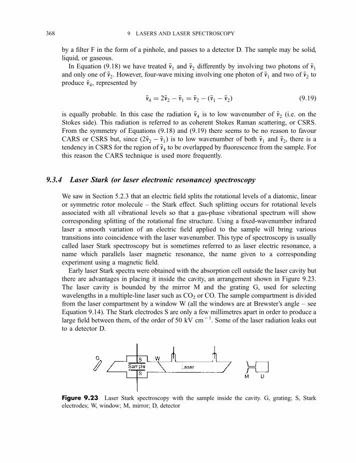
by a filter F in the form of a pinhole, and passes to a detector D. The sample may be solid,
liquid, or gaseous.
In Equation (9.18) we have treated ~nn1 and ~nn2 differently by involving two photons of ~nn1and only one of ~nn2. However, four-wave mixing involving one photon of ~nn1 and two of ~nn2 toproduce ~nn4, represented by
~nn4 ¼ 2~nn2 � ~nn1 ¼ ~nn2 � ð~nn1 � ~nn2Þ ð9:19Þ
is equally probable. In this case the radiation ~nn4 is to low wavenumber of ~nn2 (i.e. on the
Stokes side). This radiation is referred to as coherent Stokes Raman scattering, or CSRS.
From the symmetry of Equations (9.18) and (9.19) there seems to be no reason to favour
CARS or CSRS but, since ð2~nn2 � ~nn1Þ is to low wavenumber of both ~nn1 and ~nn2, there is a
tendency in CSRS for the region of ~nn4 to be overlapped by fluorescence from the sample. For
this reason the CARS technique is used more frequently.
9.3.4 Laser Stark (or laser electronic resonance) spectroscopy
We saw in Section 5.2.3 that an electric field splits the rotational levels of a diatomic, linear
or symmetric rotor molecule – the Stark effect. Such splitting occurs for rotational levels
associated with all vibrational levels so that a gas-phase vibrational spectrum will show
corresponding splitting of the rotational fine structure. Using a fixed-wavenumber infrared
laser a smooth variation of an electric field applied to the sample will bring various
transitions into coincidence with the laser wavenumber. This type of spectroscopy is usually
called laser Stark spectroscopy but is sometimes referred to as laser electric resonance, a
name which parallels laser magnetic resonance, the name given to a corresponding
experiment using a magnetic field.
Early laser Stark spectra were obtained with the absorption cell outside the laser cavity but
there are advantages in placing it inside the cavity, an arrangement shown in Figure 9.23.
The laser cavity is bounded by the mirror M and the grating G, used for selecting
wavelengths in a multiple-line laser such as CO2 or CO. The sample compartment is divided
from the laser compartment by a window W (all the windows are at Brewster’s angle – see
Equation 9.14). The Stark electrodes S are only a few millimetres apart in order to produce a
large field between them, of the order of 50 kV cm71. Some of the laser radiation leaks out
to a detector D.
Figure 9.23 Laser Stark spectroscopy with the sample inside the cavity. G, grating; S, Stark
electrodes; W, window; M, mirror; D, detector
368 9 LASERS AND LASER SPECTROSCOPY
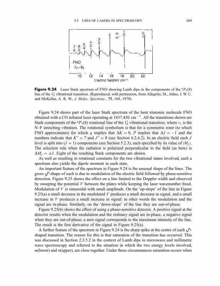
Figure 9.24 shows part of the laser Stark spectrum of the bent triatomic molecule FNO
obtained with a CO infrared laser operating at 1837.430 cm71. All the transitions shown are
Stark components of the qP7ð8Þ rotational line of the 110 vibrational transition, where n1 is theN–F stretching vibration. The rotational symbolism is that for a symmetric rotor (to which
FNO approximates) for which q implies that DK ¼ 0, P implies that DJ ¼ �1 and the
numbers indicate that K 00 ¼ 7 and J 00 ¼ 8 (see Section 6.2.4.2). In an electric field each J
level is split into ðJ þ 1Þ components (see Section 5.2.3), each specified by its value of jMJ j.The selection rule when the radiation is polarized perpendicular to the field (as here) is
DMJ ¼ �1. Eight of the resulting Stark components are shown.
As well as resulting in rotational constants for the two vibrational states involved, such a
spectrum also yields the dipole moment in each state.
An important feature of the spectrum in Figure 9.24 is the unusual shape of the lines. The
gross -shape of each is due to modulation of the electric field followed by phase-sensitive
detection. Figure 9.25 shows the effect on a line limited to the Doppler width and observed
by sweeping the potential V between the plates while keeping the laser wavenumber fixed.
Modulation of V is sinusoidal with small amplitude. On the ‘up-slope’ of the line in Figure
9.25(a) a small decrease in the modulated V produces a small decrease in signal, and a small
increase in V produces a small increase in signal: in other words the modulation and the
signal are in-phase. Similarly, on the ‘down-slope’ of the line they are out-of-phase.
Figure 9.25(b) shows the effect of using a phase-sensitive detector. A positive signal at the
detector results when the modulation and the ordinary signal are in-phase, a negative signal
when they are out-of-phase; a zero signal corresponds to the maximum intensity of the line.
The result is the first derivative of the signal in Figure 9.25(a).
A further feature of the spectrum in Figure 9.24 is the sharp spike at the centre of each -
shaped transition. The reason for this is that saturation of the transition has occurred. This
was discussed in Section 2.3.5.2 in the context of Lamb dips in microwave and millimetre
wave spectroscopy and referred to the situation in which the two energy levels involved,
m(lower) and n(upper), are close together. Under these circumstances saturation occurs when
Figure 9.24 Laser Stark spectrum of FNO showing Lamb dips in the components of the qP7ð8Þline of the 110 vibrational transition. (Reproduced, with permission, from Allegrini, M., Johns, J. W. C.
and McKellar, A. R. W., J. Molec. Spectrosc., 73, 168, 1978)
9.3 USES OF LASERS IN SPECTROSCOPY 369
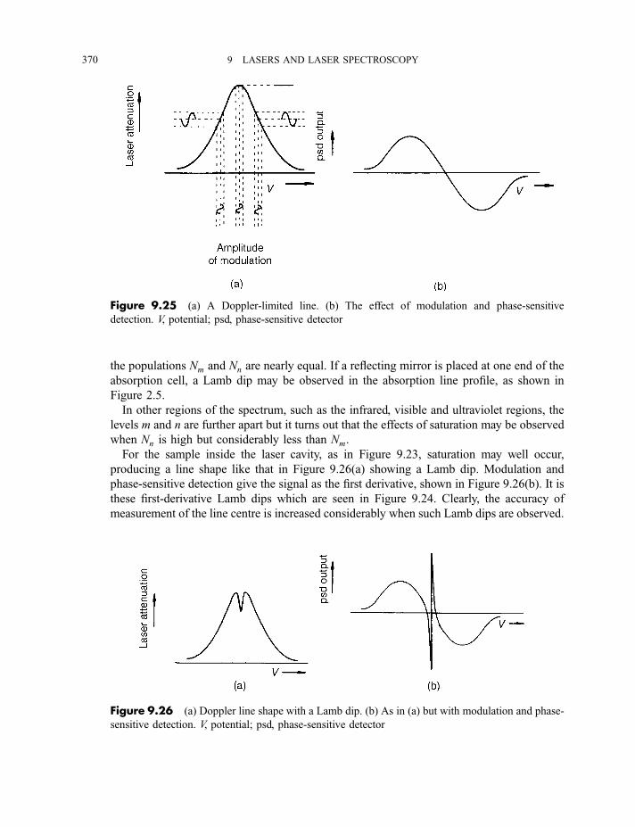
the populations Nm and Nn are nearly equal. If a reflecting mirror is placed at one end of the
absorption cell, a Lamb dip may be observed in the absorption line profile, as shown in
Figure 2.5.
In other regions of the spectrum, such as the infrared, visible and ultraviolet regions, the
levels m and n are further apart but it turns out that the effects of saturation may be observed
when Nn is high but considerably less than Nm.
For the sample inside the laser cavity, as in Figure 9.23, saturation may well occur,
producing a line shape like that in Figure 9.26(a) showing a Lamb dip. Modulation and
phase-sensitive detection give the signal as the first derivative, shown in Figure 9.26(b). It is
these first-derivative Lamb dips which are seen in Figure 9.24. Clearly, the accuracy of
measurement of the line centre is increased considerably when such Lamb dips are observed.
Figure 9.26 (a) Doppler line shape with a Lamb dip. (b) As in (a) but with modulation and phase-
sensitive detection. V, potential; psd, phase-sensitive detector
Figure 9.25 (a) A Doppler-limited line. (b) The effect of modulation and phase-sensitive
detection. V, potential; psd, phase-sensitive detector
370 9 LASERS AND LASER SPECTROSCOPY
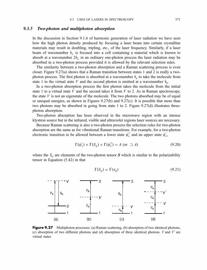
9.3.5 Two-photon and multiphoton absorption
In the discussion in Section 9.1.6 of harmonic generation of laser radiation we have seen
how the high photon density produced by focusing a laser beam into certain crystalline
materials may result in doubling, tripling, etc., of the laser frequency. Similarly, if a laser
beam of wavenumber ~nnL is focused into a cell containing a material which is known to
absorb at a wavenumber 2~nnL in an ordinary one-photon process the laser radiation may be
absorbed in a two-photon process provided it is allowed by the relevant selection rules.
The similarity between a two-photon absorption and a Raman scattering process is even
closer. Figure 9.27(a) shows that a Raman transition between states 1 and 2 is really a two-
photon process. The first photon is absorbed at a wavenumber ~nna to take the molecule from
state 1 to the virtual state V and the second photon is emitted at a wavenumber ~nnb.In a two-photon absorption process the first photon takes the molecule from the initial
state 1 to a virtual state V and the second takes it from V to 2. As in Raman spectroscopy,
the state V is not an eigenstate of the molecule. The two photons absorbed may be of equal
or unequal energies, as shown in Figures 9.27(b) and 9.27(c). It is possible that more than
two photons may be absorbed in going from state 1 to 2. Figure 9.27(d) illustrates three-
photon absorption.
Two-photon absorption has been observed in the microwave region with an intense
klystron source but in the infrared, visible and ultraviolet regions laser sources are necessary.
Because Raman scattering is also a two-photon process the selection rules for two-photon
absorption are the same as for vibrational Raman transitions. For example, for a two-photon
electronic transition to be allowed between a lower state c00e and an upper state c0e,
Gðc0eÞ � GðSijÞ � Gðc00e Þ ¼ A ðor � AÞ ð9:20Þ
where the Sij are elements of the two-photon tensor S which is similar to the polarizability
tensor in Equation (5.42) in that
GðSijÞ ¼ GðaijÞ ð9:21Þ
Figure 9.27 Multiphoton processes: (a) Raman scattering, (b) absorption of two identical photons,
(c) absorption of two different photons and (d) absorption of three identical photons. V and V 0 arevirtual states
9.3 USES OF LASERS IN SPECTROSCOPY 371
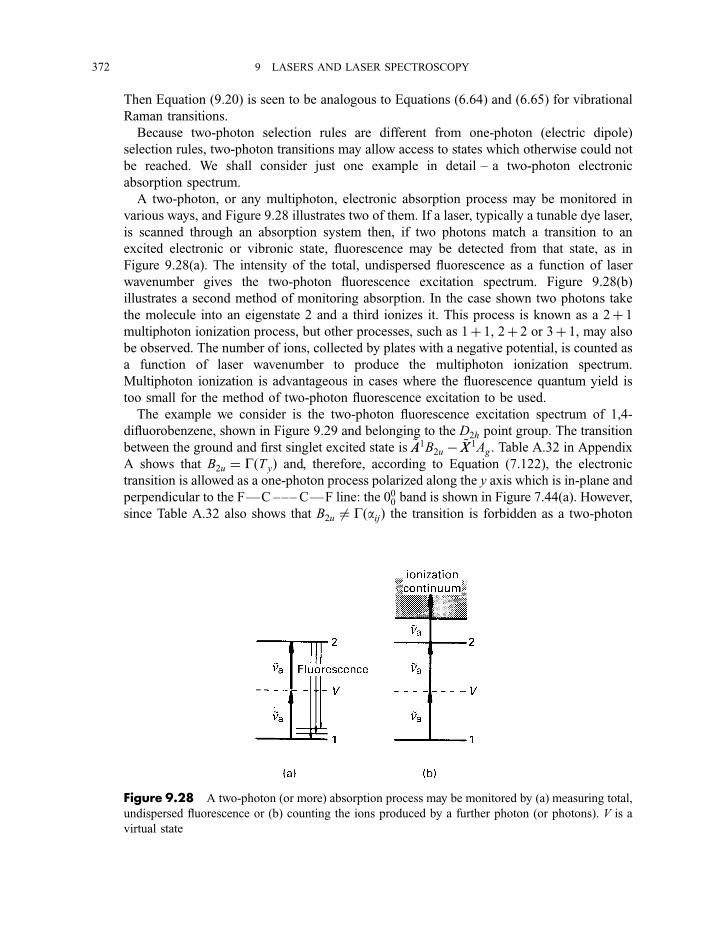
Then Equation (9.20) is seen to be analogous to Equations (6.64) and (6.65) for vibrational
Raman transitions.
Because two-photon selection rules are different from one-photon (electric dipole)
selection rules, two-photon transitions may allow access to states which otherwise could not
be reached. We shall consider just one example in detail – a two-photon electronic
absorption spectrum.
A two-photon, or any multiphoton, electronic absorption process may be monitored in
various ways, and Figure 9.28 illustrates two of them. If a laser, typically a tunable dye laser,
is scanned through an absorption system then, if two photons match a transition to an
excited electronic or vibronic state, fluorescence may be detected from that state, as in
Figure 9.28(a). The intensity of the total, undispersed fluorescence as a function of laser
wavenumber gives the two-photon fluorescence excitation spectrum. Figure 9.28(b)
illustrates a second method of monitoring absorption. In the case shown two photons take
the molecule into an eigenstate 2 and a third ionizes it. This process is known as a 2þ 1
multiphoton ionization process, but other processes, such as 1þ 1, 2þ 2 or 3þ 1, may also
be observed. The number of ions, collected by plates with a negative potential, is counted as
a function of laser wavenumber to produce the multiphoton ionization spectrum.
Multiphoton ionization is advantageous in cases where the fluorescence quantum yield is
too small for the method of two-photon fluorescence excitation to be used.
The example we consider is the two-photon fluorescence excitation spectrum of 1,4-
difluorobenzene, shown in Figure 9.29 and belonging to the D2h point group. The transition
between the ground and first singlet excited state is ~AA1B2u � ~XX 1Ag. Table A.32 in Appendix
A shows that B2u ¼ GðTyÞ and, therefore, according to Equation (7.122), the electronic
transition is allowed as a one-photon process polarized along the y axis which is in-plane and
perpendicular to the F—C ––– C—F line: the 000 band is shown in Figure 7.44(a). However,
since Table A.32 also shows that B2u 6¼ GðaijÞ the transition is forbidden as a two-photon
Figure 9.28 A two-photon (or more) absorption process may be monitored by (a) measuring total,
undispersed fluorescence or (b) counting the ions produced by a further photon (or photons). V is a
virtual state
372 9 LASERS AND LASER SPECTROSCOPY
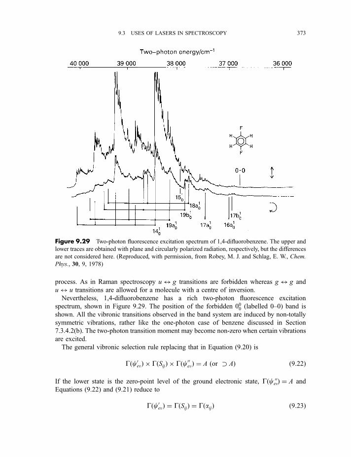
process. As in Raman spectroscopy u$ g transitions are forbidden whereas g$ g and
u$ u transitions are allowed for a molecule with a centre of inversion.
Nevertheless, 1,4-difluorobenzene has a rich two-photon fluorescence excitation
spectrum, shown in Figure 9.29. The position of the forbidden 000 (labelled 0–0) band is
shown. All the vibronic transitions observed in the band system are induced by non-totally
symmetric vibrations, rather like the one-photon case of benzene discussed in Section
7.3.4.2(b). The two-photon transition moment may become non-zero when certain vibrations
are excited.
The general vibronic selection rule replacing that in Equation (9.20) is
Gðc0evÞ � GðSijÞ � Gðc00evÞ ¼ A ðor � AÞ ð9:22Þ
If the lower state is the zero-point level of the ground electronic state, Gðcev00Þ ¼ A and
Equations (9.22) and (9.21) reduce to
Gðc0evÞ ¼ GðSijÞ ¼ GðaijÞ ð9:23Þ
Figure 9.29 Two-photon fluorescence excitation spectrum of 1,4-difluorobenzene. The upper and
lower traces are obtained with plane and circularly polarized radiation, respectively, but the differences
are not considered here. (Reproduced, with permission, from Robey, M. J. and Schlag, E. W., Chem.
Phys., 30, 9, 1978)
9.3 USES OF LASERS IN SPECTROSCOPY 373
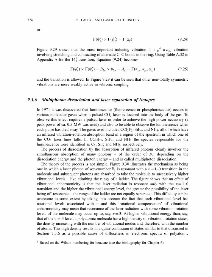
or
Gðce0Þ � Gðcv
0Þ ¼ GðaijÞ ð9:24Þ
Figure 9.29 shows that the most important inducing vibration is n14,4 a b2u vibration
involving stretching and contracting of alternate C–C bonds in the ring. Using Table A.32 in
Appendix A for the 1410 transition, Equation (9.24) becomes
Gðc0eÞ � Gðc0vÞ ¼ B2u � b2u ¼ Ag ¼ Gðaxx; ayy; azzÞ ð9:25Þ
and the transition is allowed. In Figure 9.29 it can be seen that other non-totally symmetric
vibrations are more weakly active in vibronic coupling.
9.3.6 Multiphoton dissociation and laser separation of isotopes
In 1971 it was discovered that luminescence (fluorescence or phosphorescence) occurs in
various molecular gases when a pulsed CO2 laser is focused into the body of the gas. To
observe this effect requires a pulsed laser in order to achieve the high power necessary (a
peak power of ca. 0.5 MW was used) and also to be able to observe the luminescence when
each pulse has died away. The gases used included CCl2F2, SiF4, and NH3, all of which have
an infrared vibration–rotation absorption band in a region of the spectrum in which one of
the CO2 laser lines falls. In CCl2F2, SiF4, and NH3 the species responsible for the
luminescence were identified as C2, SiF, and NH2, respectively.
The process of dissociation by the absorption of infrared photons clearly involves the
simultaneous absorption of many photons – of the order of 30, depending on the
dissociation energy and the photon energy – and is called multiphoton dissociation.
The theory of the process is not simple. Figure 9.30 illustrates the mechanism as being
one in which a laser photon of wavenumber ~nnL is resonant with a v¼ 1–0 transition in the
molecule and subsequent photons are absorbed to take the molecule to successively higher
vibrational levels – like climbing the rungs of a ladder. The figure shows that an effect of
vibrational anharmonicity is that the laser radiation is resonant only with the v¼ 1–0
transition and the higher the vibrational energy level, the greater the possibility of the laser
being off-resonance – the rungs of the ladder are not equally separated. This difficulty can be
overcome to some extent by taking into account the fact that each vibrational level has
rotational levels associated with it and this ‘rotational compensation’ of vibrational
anharmonicity may mean that resonance of the laser radiation with some vibration–rotation
levels of the molecule may occur up to, say, v¼ 3. At higher vibrational energy than, say,
that of the v ¼ 3 level, a polyatomic molecule has a high density of vibration–rotation states,
the density increasing with the number of vibrational modes and, therefore, with the number
of atoms. This high density results in a quasi-continuum of states similar to that discussed in
Section 7.3.6 as a possible cause of diffuseness in electronic spectra of polyatomic
4 Based on the Wilson numbering for benzene (see the bibliography for Chapter 6).
374 9 LASERS AND LASER SPECTROSCOPY
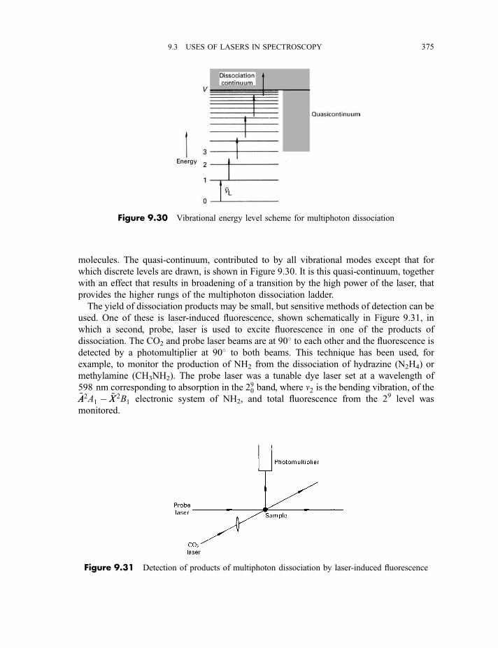
molecules. The quasi-continuum, contributed to by all vibrational modes except that for
which discrete levels are drawn, is shown in Figure 9.30. It is this quasi-continuum, together
with an effect that results in broadening of a transition by the high power of the laser, that
provides the higher rungs of the multiphoton dissociation ladder.
The yield of dissociation products may be small, but sensitive methods of detection can be
used. One of these is laser-induced fluorescence, shown schematically in Figure 9.31, in
which a second, probe, laser is used to excite fluorescence in one of the products of
dissociation. The CO2 and probe laser beams are at 90� to each other and the fluorescence is
detected by a photomultiplier at 90� to both beams. This technique has been used, for
example, to monitor the production of NH2 from the dissociation of hydrazine (N2H4) or
methylamine (CH3NH2). The probe laser was a tunable dye laser set at a wavelength of
598 nm corresponding to absorption in the 290 band, where n2 is the bending vibration, of the~AA2A1 � ~XX 2B1 electronic system of NH2, and total fluorescence from the 29 level was
monitored.
Figure 9.30 Vibrational energy level scheme for multiphoton dissociation
Figure 9.31 Detection of products of multiphoton dissociation by laser-induced fluorescence
9.3 USES OF LASERS IN SPECTROSCOPY 375
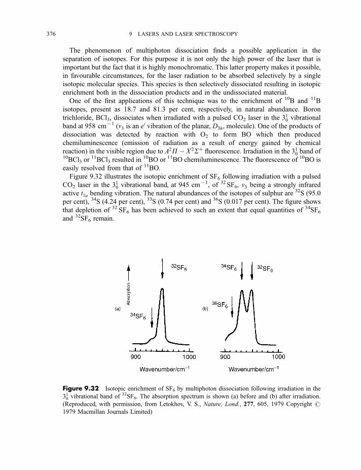
The phenomenon of multiphoton dissociation finds a possible application in the
separation of isotopes. For this purpose it is not only the high power of the laser that is
important but the fact that it is highly monochromatic. This latter property makes it possible,
in favourable circumstances, for the laser radiation to be absorbed selectively by a single
isotopic molecular species. This species is then selectively dissociated resulting in isotopic
enrichment both in the dissociation products and in the undissociated material.
One of the first applications of this technique was to the enrichment of 10B and 11B
isotopes, present as 18.7 and 81.3 per cent, respectively, in natural abundance. Boron
trichloride, BCl3, dissociates when irradiated with a pulsed CO2 laser in the 310 vibrational
band at 958 cm71 (n3 is an e0 vibration of the planar, D3h, molecule). One of the products of
dissociation was detected by reaction with O2 to form BO which then produced
chemiluminescence (emission of radiation as a result of energy gained by chemical
reaction) in the visible region due to A2P� X 2Sþ fluorescence. Irradiation in the 310 band of10BCl3 or
11BCl3 resulted in 10BO or 11BO chemiluminescence. The fluorescence of 10BO is
easily resolved from that of 11BO.
Figure 9.32 illustrates the isotopic enrichment of SF6 following irradiation with a pulsed
CO2 laser in the 310 vibrational band, at 945 cm71, of 32SF6, n3 being a strongly infrared
active t1u bending vibration. The natural abundances of the isotopes of sulphur are 32S (95.0
per cent), 34S (4.24 per cent), 33S (0.74 per cent) and 36S (0.017 per cent). The figure shows
that depletion of 32 SF6 has been achieved to such an extent that equal quantities of 34SF6and 32SF6 remain.
Figure 9.32 Isotopic enrichment of SF6 by multiphoton dissociation following irradiation in the
310 vibrational band of 32SF6. The absorption spectrum is shown (a) before and (b) after irradiation.
(Reproduced, with permission, from Letokhov, V. S., Nature, Lond., 277, 605, 1979 Copyright #1979 Macmillan Journals Limited)
376 9 LASERS AND LASER SPECTROSCOPY
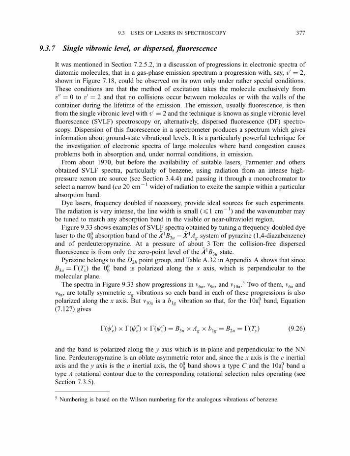
9.3.7 Single vibronic level, or dispersed, fluorescence
It was mentioned in Section 7.2.5.2, in a discussion of progressions in electronic spectra of
diatomic molecules, that in a gas-phase emission spectrum a progression with, say, v0 ¼ 2,
shown in Figure 7.18, could be observed on its own only under rather special conditions.
These conditions are that the method of excitation takes the molecule exclusively from
v00 ¼ 0 to v0 ¼ 2 and that no collisions occur between molecules or with the walls of the
container during the lifetime of the emission. The emission, usually fluorescence, is then
from the single vibronic level with v0 ¼ 2 and the technique is known as single vibronic level
fluorescence (SVLF) spectroscopy or, alternatively, dispersed fluorescence (DF) spectro-
scopy. Dispersion of this fluorescence in a spectrometer produces a spectrum which gives
information about ground-state vibrational levels. It is a particularly powerful technique for
the investigation of electronic spectra of large molecules where band congestion causes
problems both in absorption and, under normal conditions, in emission.
From about 1970, but before the availability of suitable lasers, Parmenter and others
obtained SVLF spectra, particularly of benzene, using radiation from an intense high-
pressure xenon arc source (see Section 3.4.4) and passing it through a monochromator to
select a narrow band (ca 20 cm71 wide) of radiation to excite the sample within a particular
absorption band.
Dye lasers, frequency doubled if necessary, provide ideal sources for such experiments.
The radiation is very intense, the line width is small (41 cm71) and the wavenumber may
be tuned to match any absorption band in the visible or near-ultraviolet region.
Figure 9.33 shows examples of SVLF spectra obtained by tuning a frequency-doubled dye
laser to the 000 absorption band of the ~AA1B3u � ~XX 1Ag system of pyrazine (1,4-diazabenzene)
and of perdeuteropyrazine. At a pressure of about 3 Torr the collision-free dispersed
fluorescence is from only the zero-point level of the ~AA1B3u state.
Pyrazine belongs to the D2h point group, and Table A.32 in Appendix A shows that since
B3u ¼ GðTxÞ the 000 band is polarized along the x axis, which is perpendicular to the
molecular plane.
The spectra in Figure 9.33 show progressions in n6a, n9a, and n10a:5 Two of them, n6a and
n9a, are totally symmetric ag vibrations so each band in each of these progressions is also
polarized along the x axis. But n10a is a b1g vibration so that, for the 10a01 band, Equation
(7.127) gives
Gðc0eÞ � Gðc00e Þ � Gðc00v Þ ¼ B3u � Ag � b1g ¼ B2u ¼ GðTyÞ ð9:26Þ
and the band is polarized along the y axis which is in-plane and perpendicular to the NN
line. Perdeuteropyrazine is an oblate asymmetric rotor and, since the x axis is the c inertial
axis and the y axis is the a inertial axis, the 000 band shows a type C and the 10a01 band a
type A rotational contour due to the corresponding rotational selection rules operating (see
Section 7.3.5).
5 Numbering is based on the Wilson numbering for the analogous vibrations of benzene.
9.3 USES OF LASERS IN SPECTROSCOPY 377
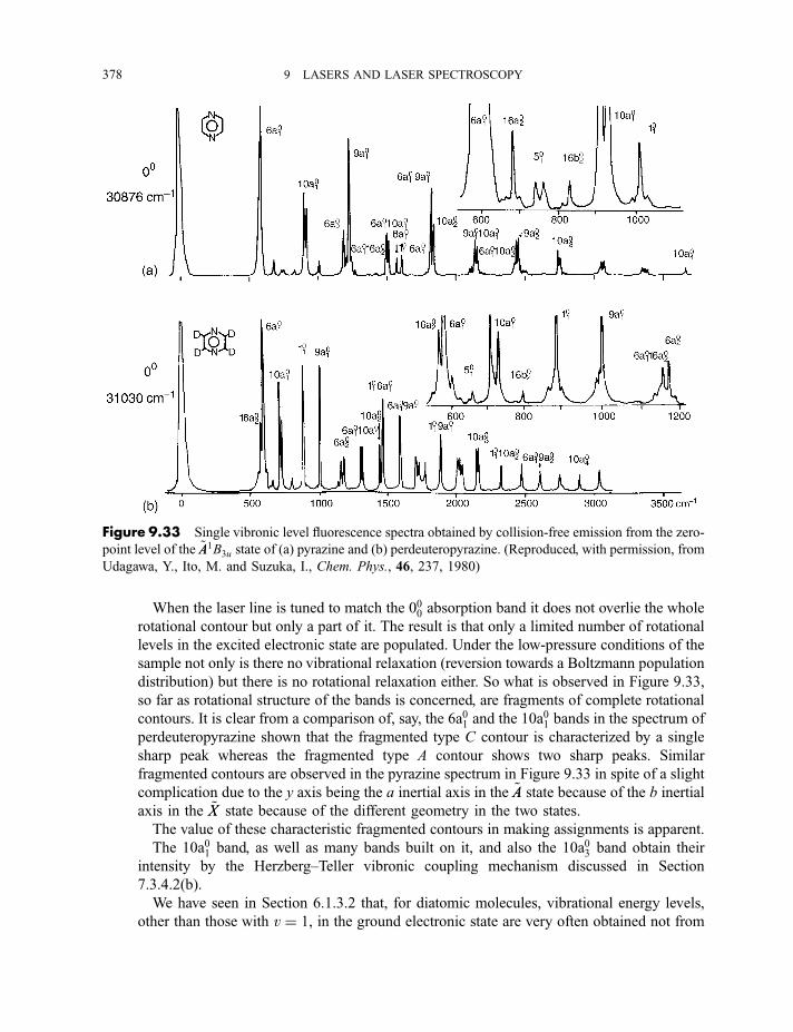
When the laser line is tuned to match the 000 absorption band it does not overlie the whole
rotational contour but only a part of it. The result is that only a limited number of rotational
levels in the excited electronic state are populated. Under the low-pressure conditions of the
sample not only is there no vibrational relaxation (reversion towards a Boltzmann population
distribution) but there is no rotational relaxation either. So what is observed in Figure 9.33,
so far as rotational structure of the bands is concerned, are fragments of complete rotational
contours. It is clear from a comparison of, say, the 6a01 and the 10a01 bands in the spectrum of
perdeuteropyrazine shown that the fragmented type C contour is characterized by a single
sharp peak whereas the fragmented type A contour shows two sharp peaks. Similar
fragmented contours are observed in the pyrazine spectrum in Figure 9.33 in spite of a slight
complication due to the y axis being the a inertial axis in the ~AA state because of the b inertial
axis in the ~XX state because of the different geometry in the two states.
The value of these characteristic fragmented contours in making assignments is apparent.
The 10a01 band, as well as many bands built on it, and also the 10a03 band obtain their
intensity by the Herzberg–Teller vibronic coupling mechanism discussed in Section
7.3.4.2(b).
We have seen in Section 6.1.3.2 that, for diatomic molecules, vibrational energy levels,
other than those with v ¼ 1, in the ground electronic state are very often obtained not from
Figure 9.33 Single vibronic level fluorescence spectra obtained by collision-free emission from the zero-
point level of the ~AA1B3u state of (a) pyrazine and (b) perdeuteropyrazine. (Reproduced, with permission, from
Udagawa, Y., Ito, M. and Suzuka, I., Chem. Phys., 46, 237, 1980)
378 9 LASERS AND LASER SPECTROSCOPY
vibrational spectroscopy but from electronic emission spectroscopy. In the emission process
we rely on the Franck–Condon principle to allow access to high-lying vibrational levels in
the ground electronic state. From these levels the potential energy curve may be constructed.
If we require similar information regarding the ground state potential energy surface in a
polyatomic molecule the electronic emission spectrum may again provide valuable
information: SVLF spectroscopy is a particularly powerful technique for providing it.
9.3.8 Light detection and ranging (LIDAR)
LIDAR is an acronym for ‘light detection and ranging’. The technique uses the same
principles as RADAR, an acronym for ‘radiowave detection and ranging’. RADAR is used
for measuring the distance of an object from an observer. The time taken for radiowave
radiation to travel to and from the object, which reflects or backscatters the radiation, is
readily translated into a measurement of distance.
In its use for range finding (i.e. measuring the distance of an object from an observer)
LIDAR works in a similar way except that the source of radiation is a pulsed laser and the
wavelength lies in the infrared, visible or ultraviolet region. Laser range finding is used by
the military to determine the distance of an object to be attacked, and by the police in
detecting speeding motorists. The speed of a car is determined by timing a pulse of radiation
emitted by the LIDAR gun and reflected back to a detector which is also contained in the
gun. The speed of the car is obtained by timing successive pulses.
LIDAR provides a very powerful technique for investigations of the earth’s atmosphere
both in the troposphere, up to 14 km, and the stratosphere, in the range 18–50 km above the
surface. The components of the atmosphere may be in the form of liquid droplets (cloud),
particles (aerosol) or a gas. The LIDAR device may be terrestrial, installed in an aeroplane
or space-based and, like the gun detecting a speeding car, is a combination of a pulsed laser
source and a detector for measuring the reflected or backscattered radiation. Its use as a
range finder allows the measurement of distances of clouds, particle aerosols or gaseous
components from the LIDAR device. The height distribution is obtained by making
observations at different time intervals for the pulse to return to the detector.
It is the use of LIDAR devices as tools for spectroscopic measurements on the various
gases present in the atmosphere which concerns us here. These include ozone, carbon
dioxide, the CFCs (chlorofluorocarbons, such as CFC-11, trichlorofluoromethane, and CFC-
12, dichlorodifluoromethane, used as refrigerants) and all those molecules regarded as
atmospheric pollutants.
Figure 9.34 shows a typical LIDAR device. Radiation from the laser, in the form of a
highly parallel beam, is reflected by the mirror M1 and directed to the part of the atmosphere
being investigated. The choice of the return time for the backscattered laser pulse is a
consequence of the choice of height in the atmosphere at which measurements are required.
The device commonly used for collecting the backscattered light is a Cassagrain telescope
consisting of a large concave mirror M2, which collects the radiation, and a further mirror
M3 which reflects and focuses it onto the detector.
9.3 USES OF LASERS IN SPECTROSCOPY 379
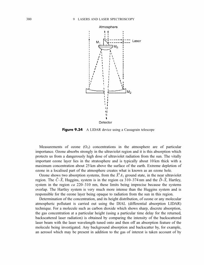
Measurements of ozone (O3) concentrations in the atmosphere are of particular
importance. Ozone absorbs strongly in the ultraviolet region and it is this absorption which
protects us from a dangerously high dose of ultraviolet radiation from the sun. The vitally
important ozone layer lies in the stratosphere and is typically about 10 km thick with a
maximum concentration about 25 km above the surface of the earth. Extreme depletion of
ozone in a localised part of the atmosphere creates what is known as an ozone hole.
Ozone shows two absorption systems, from the X1A1 ground state, in the near ultraviolet
region. The C–X, Huggins, system is in the region ca 310–374 nm and the D–X, Hartley,
system in the region ca 220–310 nm, these limits being imprecise because the systems
overlap. The Hartley system is very much more intense than the Huggins system and is
responsible for the ozone layer being opaque to radiation from the sun in this region.
Determination of the concentration, and its height distribution, of ozone or any molecular
atmospheric pollutant is carried out using the DIAL (differential absorption LIDAR)
technique. For a molecule such as carbon dioxide which shows sharp, discrete absorption,
the gas concentration at a particular height (using a particular time delay for the returned,
backscattered laser radiation) is obtained by comparing the intensity of the backscattered
laser beam with the laser wavelength tuned onto and then off an absorption feature of the
molecule being investigated. Any background absorption and backscatter by, for example,
an aerosol which may be present in addition to the gas of interest is taken account of by
Figure 9.34 A LIDAR device using a Cassagrain telescope
380 9 LASERS AND LASER SPECTROSCOPY
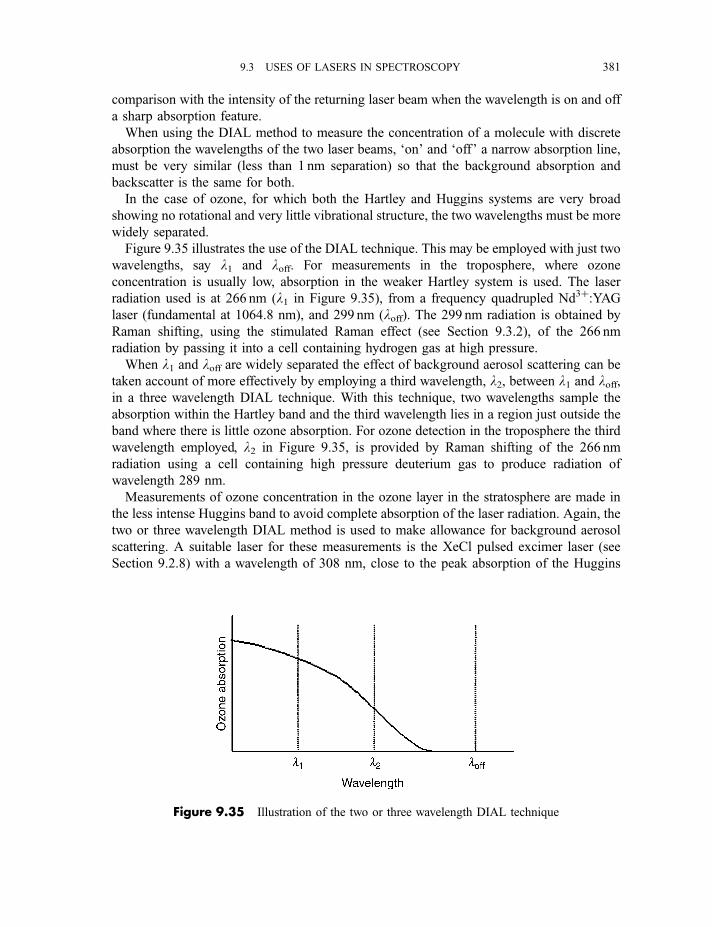
comparison with the intensity of the returning laser beam when the wavelength is on and off
a sharp absorption feature.
When using the DIAL method to measure the concentration of a molecule with discrete
absorption the wavelengths of the two laser beams, ‘on’ and ‘off’ a narrow absorption line,
must be very similar (less than 1 nm separation) so that the background absorption and
backscatter is the same for both.
In the case of ozone, for which both the Hartley and Huggins systems are very broad
showing no rotational and very little vibrational structure, the two wavelengths must be more
widely separated.
Figure 9.35 illustrates the use of the DIAL technique. This may be employed with just two
wavelengths, say l1 and loff. For measurements in the troposphere, where ozone
concentration is usually low, absorption in the weaker Hartley system is used. The laser
radiation used is at 266 nm (l1 in Figure 9.35), from a frequency quadrupled Nd3þ:YAGlaser (fundamental at 1064.8 nm), and 299 nm (loff). The 299 nm radiation is obtained by
Raman shifting, using the stimulated Raman effect (see Section 9.3.2), of the 266 nm
radiation by passing it into a cell containing hydrogen gas at high pressure.
When l1 and loff are widely separated the effect of background aerosol scattering can be
taken account of more effectively by employing a third wavelength, l2, between l1 and loff,in a three wavelength DIAL technique. With this technique, two wavelengths sample the
absorption within the Hartley band and the third wavelength lies in a region just outside the
band where there is little ozone absorption. For ozone detection in the troposphere the third
wavelength employed, l2 in Figure 9.35, is provided by Raman shifting of the 266 nm
radiation using a cell containing high pressure deuterium gas to produce radiation of
wavelength 289 nm.
Measurements of ozone concentration in the ozone layer in the stratosphere are made in
the less intense Huggins band to avoid complete absorption of the laser radiation. Again, the
two or three wavelength DIAL method is used to make allowance for background aerosol
scattering. A suitable laser for these measurements is the XeCl pulsed excimer laser (see
Section 9.2.8) with a wavelength of 308 nm, close to the peak absorption of the Huggins
Figure 9.35 Illustration of the two or three wavelength DIAL technique
9.3 USES OF LASERS IN SPECTROSCOPY 381
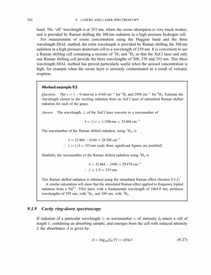
band. The ‘off’ wavelength is at 353 nm, where the ozone absorption is very much weaker,
and is provided by Raman shifting the 308 nm radiation in a high pressure hydrogen cell.
For measurement of ozone concentration using the Huggins band and the three
wavelength DIAL method, the extra wavelength is provided by Raman shifting the 308 nm
radiation in a high pressure deuterium cell to a wavelength of 339 nm. It is convenient to use
a Raman shifting cell containing a mixture of 1H2 and2H2 so that the XeCl laser and only
one Raman shifting cell provide the three wavelengths of 308, 339 and 353 nm. This three
wavelength DIAL method has proved particularly useful when the aerosol concentration is
high, for example when the ozone layer is seriously contaminated as a result of volcanic
eruption.
Worked example 9.3
Question. The v ¼ 1� 0 interval is 4160 cm�1 for 1H2 and 2990 cm�1 for 2H2. Estimate the
wavelength closest to the exciting radiation from an XeCl laser of stimulated Raman shifted
radiation for each of the gases.
Answer. The wavelength, l, of the XeCl laser converts to a wavenumber of
~nn ¼ 1=l ¼ 1=308 nm ¼ 32 468 cm�1
The wavenumber of the Raman shifted radiation, using 1H2, is
~nn ¼ 32 468� 4160 ¼ 28 308 cm�1
; l ¼ 1=~nn ¼ 353 nm (only three significant figures are justified)
Similarly, the wavenumber of the Raman shifted radiation using 2H2 is
~nn ¼ 32 468� 2990 ¼ 29 478 cm�1
; l ¼ 1=~nn ¼ 339 nm
This Raman shifted radiation is obtained using the stimulated Raman effect (Section 9.3.2)
A similar calculation will show that the stimulated Raman effect applied to frequency tripled
radiation from a Nd3þ : YAG laser, with a fundamental wavelength of 1064.8 nm, produces
wavelengths of 299 nm, with 1H2, and 289 nm, with 2H2.
9.3.9 Cavity ring-down spectroscopy
If radiation of a particular wavelength l, or wavenumber n, of intensity I0 enters a cell of
length ‘, containing an absorbing sample, and emerges from the cell with reduced intensity
I, the absorbance A is given by:
A ¼ log10ðI0=I Þ ¼ eð~nnÞc‘ ð9:27Þ
382 9 LASERS AND LASER SPECTROSCOPY
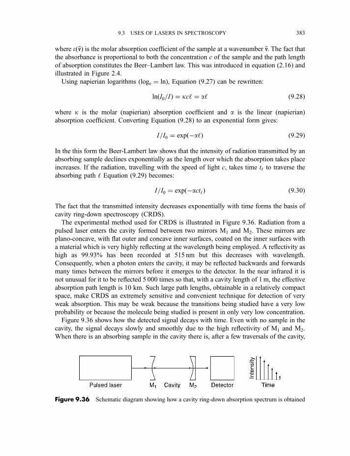
where e(~nn) is the molar absorption coefficient of the sample at a wavenumber ~nn. The fact thatthe absorbance is proportional to both the concentration c of the sample and the path length
of absorption constitutes the Beer–Lambert law. This was introduced in equation (2.16) and
illustrated in Figure 2.4.
Using napierian logarithms (loge ¼ ln), Equation (9.27) can be rewritten:
lnðI0=I Þ ¼ kc‘ ¼ a‘ ð9:28Þ
where k is the molar (napierian) absorption coefficient and a is the linear (napierian)
absorption coefficient. Converting Equation (9.28) to an exponential form gives:
I=I0 ¼ expð�a‘Þ ð9:29Þ
In the this form the Beer-Lambert law shows that the intensity of radiation transmitted by an
absorbing sample declines exponentially as the length over which the absorption takes place
increases. If the radiation, travelling with the speed of light c, takes time t‘ to traverse the
absorbing path ‘ Equation (9.29) becomes:
I=I0 ¼ expð�act‘Þ ð9:30Þ
The fact that the transmitted intensity decreases exponentially with time forms the basis of
cavity ring-down spectroscopy (CRDS).
The experimental method used for CRDS is illustrated in Figure 9.36. Radiation from a
pulsed laser enters the cavity formed between two mirrors M1 and M2. These mirrors are
plano-concave, with flat outer and concave inner surfaces, coated on the inner surfaces with
a material which is very highly reflecting at the wavelength being employed. A reflectivity as
high as 99.93% has been recorded at 515 nm but this decreases with wavelength.
Consequently, when a photon enters the cavity, it may be reflected backwards and forwards
many times between the mirrors before it emerges to the detector. In the near infrared it is
not unusual for it to be reflected 5 000 times so that, with a cavity length of 1m, the effective
absorption path length is 10 km. Such large path lengths, obtainable in a relatively compact
space, make CRDS an extremely sensitive and convenient technique for detection of very
weak absorption. This may be weak because the transitions being studied have a very low
probability or because the molecule being studied is present in only very low concentration.
Figure 9.36 shows how the detected signal decays with time. Even with no sample in the
cavity, the signal decays slowly and smoothly due to the high reflectivity of M1 and M2.
When there is an absorbing sample in the cavity there is, after a few traversals of the cavity,
Figure 9.36 Schematic diagram showing how a cavity ring-down absorption spectrum is obtained
9.3 USES OF LASERS IN SPECTROSCOPY 383
little absorption by the sample and the signal is strong. At longer times, after more
traversals, the signal decreases: Equation (9.30) shows that the rate of decrease due to
absorption is exponential. Measurement of this rate of decrease gives a very accurate value
of the linear (napierian) absorption coefficient a. The variation of a, as the wavelength of the
laser is tuned through the region in which the sample absorbs, gives the absorption
spectrum.
The pulses of radiation are said to ‘‘ring’’ backwards and forwards between the mirrors
and the time for the signal to decrease to 1/e of its original value is called the ring-down time
of the cavity: hence the name cavity ring-down spectroscopy.
We saw in Section 9.3.8 that spectroscopy, in the form of LIDAR, is a very important tool
for measuring ozone concentration directly in the atmosphere. A useful indirect method
involves the measurement of the concentration of oxygen which is formed from ozone by
photolysis:
O3! O2ða1Dg; b1Sþg Þ þ Oð1DÞ ð9:31Þ
where a and b are the lowest and second lowest excited states of O2. It was explained in
Section 7.2.4 how these states, together with the X 3S�g ground state, arise from the
. . .(sg2p)2(pu2p)
4(pg*2p)2 ground electron configuration. Photolysis by radiation from the
sun, at wavelengths below about 310 nm, produces O2 almost exclusively in the a state
whereas a wavelength as low as 193 nm produces about 23% of O2 in the b state.
Both the a1Dg7X 3S�g and the b1Sþg 7X 3S�g transitions are extremely weak. The
selection rules, discussed in Section 7.2.3, show that both transitions violate the DS ¼ 0 and
the g 7!g selection rules. In addition, the a–X transition violates the DL = 0, � 1 selection
rule and the b –X transition the þ 7!� selection rule. Spin-orbit interaction breaks down
the DS ¼ 0 selection rule to some extent. Magnetic dipole selection rules, as opposed to the
electric dipole selection rules of Section 7.2.3, allow both the a–X and b–X transitions but
only weakly.
Both the a–X and b–X transitions have long been known from absorption by the oxygen in
the earth’s atmosphere, the source of radiation being the sun and the very long path length of
oxygen overcoming their extreme weakness. For laboratory observation of these transitions,
and particularly for accurate determination of absolute absorption intensity, CRDS has
proved to be an ideal technique.
Figure 9.37 shows the first CRD spectrum to be obtained and is that of the v ¼ 1–0
vibronic band in the b–X electronic band system of O2. The length of the cavity was 1 m and
it was filled with air at atmospheric pressure containing about 20% oxygen. The rotational
selection rules for such an unusual type of transition allows a P branch, an R branch and two
Q branches: these are labelled rQ and pQ. (In general, pre-superscripts . . . o, p, q, r, s . . .indicate that DN ¼ . . .�2, �1, 0, þ1, þ2 . . . . The X 3S�g ground state of O2 belongs to the
rather unusual Hund’s case (b). In this case, the rotational (N) and electron spin (S) angular
momenta couple to give an angular momentum (J) where J ¼ N þ S, N þ S–1, . . . , |N–S |.)The pQ and P branches are labelled: the R and rQ branches form the low-wavelength group
of lines.
384 9 LASERS AND LASER SPECTROSCOPY
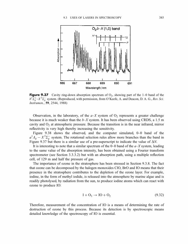
Observation, in the laboratory, of the a–X system of O2 represents a greater challenge
because it is much weaker than the b–X system. It has been observed using CRDS, a 1.5 m
cavity and O2 at atmospheric pressure. Because the transition is in the near infrared, mirror
reflectivity is very high thereby increasing the sensitivity.
Figure 9.38 shows the observed, and the computer simulated, 0–0 band of the
a1Dg7X 3S�g system. The rotational selection rules allow more branches than the band in
Figure 9.37 but there is a similar use of a pre-superscript to indicate the value of DN.It is interesting to note that a similar spectrum of the 0–0 band of the a–X system, leading
to the same value of the absorption intensity, has been obtained using a Fourier transform
spectrometer (see Section 3.3.3.2) but with an absorption path, using a multiple reflection
cell, of 129 m and half the pressure of gas.
The importance of ozone in the stratosphere has been stressed in Section 9.3.8. The fact
that ozone can be decomposed by the halogen monoxides ClO, BrO and IO means that their
presence in the stratosphere contributes to the depletion of the ozone layer. For example,
iodine, in the form of methyl iodide, is released into the atmosphere by marine algae and is
readily photolysed, by radiation from the sun, to produce iodine atoms which can react with
ozone to produce IO:
Iþ O3! IOþ O2 ð9:32Þ
Therefore, measurement of the concentration of IO is a means of determining the rate of
destruction of ozone by this process. Because its detection is by spectroscopic means
detailed knowledge of the spectroscopy of IO is essential.
Figure 9.37 Cavity ring-down absorption spectrum of O2, showing part of the 1–0 band of the
b1Sþg –X3S�g system. (Reproduced, with permission, from O’Keefe, A. and Deacon, D. A. G., Rev. Sci.
Instrumen., 59, 2544, 1988)
9.3 USES OF LASERS IN SPECTROSCOPY 385
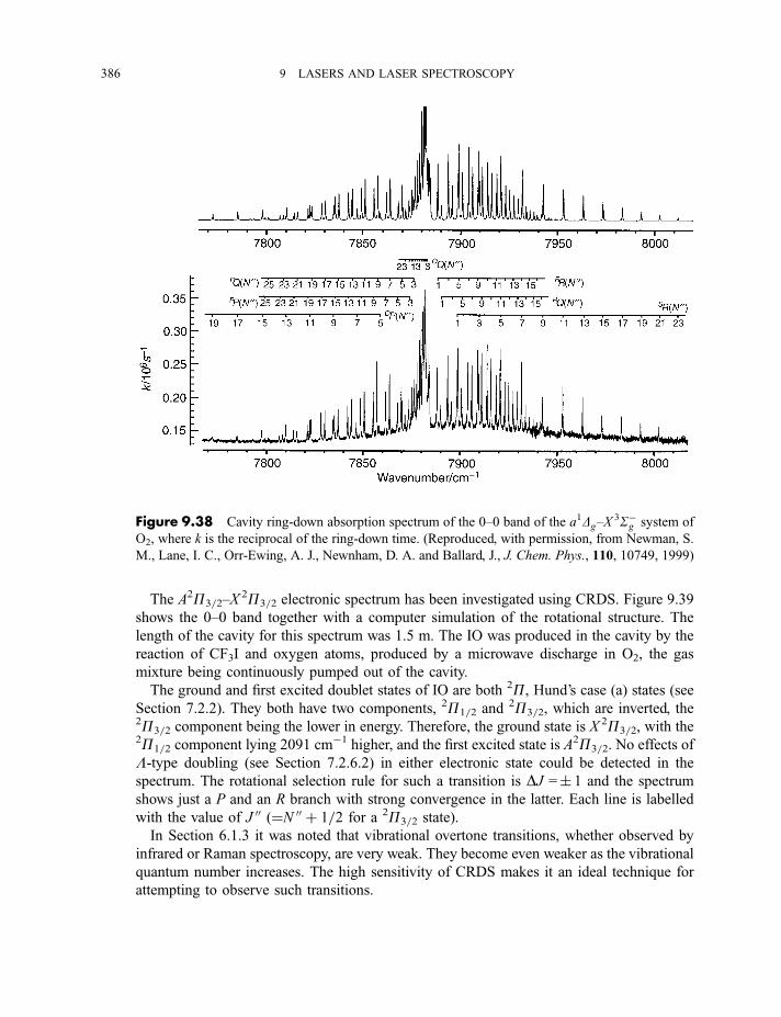
The A2P3=2–X2P3=2 electronic spectrum has been investigated using CRDS. Figure 9.39
shows the 0–0 band together with a computer simulation of the rotational structure. The
length of the cavity for this spectrum was 1.5 m. The IO was produced in the cavity by the
reaction of CF3I and oxygen atoms, produced by a microwave discharge in O2, the gas
mixture being continuously pumped out of the cavity.
The ground and first excited doublet states of IO are both 2P, Hund’s case (a) states (see
Section 7.2.2). They both have two components, 2P1=2 and2P3=2, which are inverted, the
2P3=2 component being the lower in energy. Therefore, the ground state is X 2P3=2, with the2P1=2 component lying 2091 cm�1 higher, and the first excited state is A2P3=2. No effects of
L-type doubling (see Section 7.2.6.2) in either electronic state could be detected in the
spectrum. The rotational selection rule for such a transition is DJ =� 1 and the spectrum
shows just a P and an R branch with strong convergence in the latter. Each line is labelled
with the value of J 00 (¼N 00 þ 1=2 for a 2P3=2 state).
In Section 6.1.3 it was noted that vibrational overtone transitions, whether observed by
infrared or Raman spectroscopy, are very weak. They become even weaker as the vibrational
quantum number increases. The high sensitivity of CRDS makes it an ideal technique for
attempting to observe such transitions.
Figure 9.38 Cavity ring-down absorption spectrum of the 0–0 band of the a1Dg–X3S�g system of
O2, where k is the reciprocal of the ring-down time. (Reproduced, with permission, from Newman, S.
M., Lane, I. C., Orr-Ewing, A. J., Newnham, D. A. and Ballard, J., J. Chem. Phys., 110, 10749, 1999)
386 9 LASERS AND LASER SPECTROSCOPY
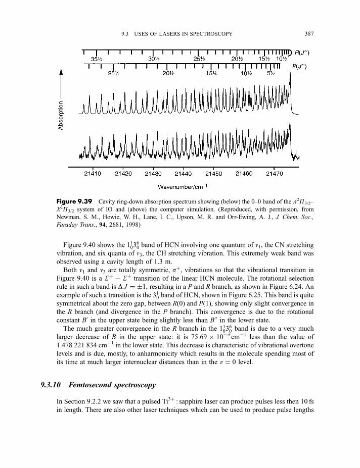
Figure 9.40 shows the 110360 band of HCN involving one quantum of n1, the CN stretching
vibration, and six quanta of n3, the CH stretching vibration. This extremely weak band was
observed using a cavity length of 1.3 m.
Both n1 and n3 are totally symmetric, sþ, vibrations so that the vibrational transition in
Figure 9.40 is a Sþ7Sþ transition of the linear HCN molecule. The rotational selection
rule in such a band is D J ¼ �1, resulting in a P and R branch, as shown in Figure 6.24. An
example of such a transition is the 310 band of HCN, shown in Figure 6.25. This band is quite
symmetrical about the zero gap, between R(0) and P(1), showing only slight convergence in
the R branch (and divergence in the P branch). This convergence is due to the rotational
constant B0 in the upper state being slightly less than B00 in the lower state.
The much greater convergence in the R branch in the 110360 band is due to a very much
larger decrease of B in the upper state: it is 75.696 10�3 cm�1 less than the value of
1.478 221 834 cm�1 in the lower state. This decrease is characteristic of vibrational overtonelevels and is due, mostly, to anharmonicity which results in the molecule spending most of
its time at much larger internuclear distances than in the v ¼ 0 level.
9.3.10 Femtosecond spectroscopy
In Section 9.2.2 we saw that a pulsed Ti3þ : sapphire laser can produce pulses less then 10 fs
in length. There are also other laser techniques which can be used to produce pulse lengths
Figure 9.39 Cavity ring-down absorption spectrum showing (below) the 0–0 band of the A2P3/2–
X2P3/2 system of IO and (above) the computer simulation. (Reproduced, with permission, from
Newman, S. M., Howie, W. H., Lane, I. C., Upson, M. R. and Orr-Ewing, A. J., J. Chem. Soc.,
Faraday Trans., 94, 2681, 1998)
9.3 USES OF LASERS IN SPECTROSCOPY 387
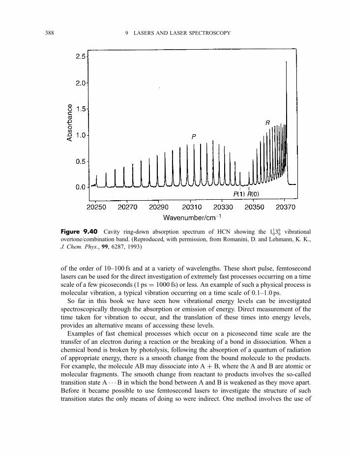
of the order of 10–100 fs and at a variety of wavelengths. These short pulse, femtosecond
lasers can be used for the direct investigation of extremely fast processes occurring on a time
scale of a few picoseconds (1 ps ¼ 1000 fs) or less. An example of such a physical process is
molecular vibration, a typical vibration occurring on a time scale of 0.1–1.0 ps.
So far in this book we have seen how vibrational energy levels can be investigated
spectroscopically through the absorption or emission of energy. Direct measurement of the
time taken for vibration to occur, and the translation of these times into energy levels,
provides an alternative means of accessing these levels.
Examples of fast chemical processes which occur on a picosecond time scale are the
transfer of an electron during a reaction or the breaking of a bond in dissociation. When a
chemical bond is broken by photolysis, following the absorption of a quantum of radiation
of appropriate energy, there is a smooth change from the bound molecule to the products.
For example, the molecule AB may dissociate into A þ B, where the A and B are atomic or
molecular fragments. The smooth change from reactant to products involves the so-called
transition state A � � �B in which the bond between A and B is weakened as they move apart.
Before it became possible to use femtosecond lasers to investigate the structure of such
transition states the only means of doing so were indirect. One method involves the use of
Figure 9.40 Cavity ring-down absorption spectrum of HCN showing the 110360 vibrational
overtone/combination band. (Reproduced, with permission, from Romanini, D. and Lehmann, K. K.,
J. Chem. Phys., 99, 6287, 1993)
388 9 LASERS AND LASER SPECTROSCOPY
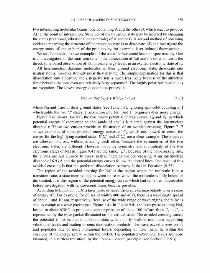
two intersecting molecular beams, one containing A and the other B, which react to produce
AB at the point of intersection. Structure of the transition state may be inferred by changing
the states (rotational, vibrational or electronic) of A and/or B. A second method of obtaining
evidence regarding the structure of the transition state is to dissociate AB and investigate the
energy states of one or both of the products by, for example, laser induced fluorescence.
We shall consider just two examples of the use of femtosecond lasers in spectroscopy. One
is an investigation of the transition state in the dissociation of NaI and the other concerns the
direct, time-based observation of vibrational energy levels in an excited electronic state of I2.
All heteronuclear diatomic molecules, in their ground electronic state, dissociate into
neutral atoms, however strongly polar they may be. The simple explanation for this is that
dissociation into a positive and a negative ion is much less likely because of the attractive
force between the ions even at a relatively large separation. The highly polar NaI molecule is
no exception. The lowest energy dissociation process is
NaI! Nað2S1=2Þ þ Ið2P3=2;2 P1=2Þ ð9:33Þ
where Na and I are in their ground states (see Table 7.1), ignoring spin-orbit coupling in I
which splits the two 2P states. Dissociation into Naþ and I� requires rather more energy.
Figure 9.41 shows, for NaI, the two lowest potential energy curves, V0 and V1, in which
potential energy V (converted to thousands of cm�1) is plotted against the internuclear
distance r. These two curves provide an illustration of an avoided crossing. Figure 7.17
shows examples of some potential energy curves of C2 which are allowed to cross: the
curves for the high-lying excited states E1Sþg and D1Sþu are a clear example. These curves
are allowed to cross, without affecting each other, because the symmetries of the two
electronic states are different. However, both the symmetry and multiplicity of the two
electronic states of NaI in Figure 9.41 are the same, 1Sþ. Because of the non-crossing rule,
the curves are not allowed to cross: instead there is avoided crossing at an internuclear
distance of 6.93 A and the potential energy curves follow the dotted lines. One result of this
avoided crossing is that the preferred dissociation pathway is that in Equation (9.33).
The region of the avoided crossing for NaI is the region where the molecule is in a
transition state, a state intermediate between those in which the molecule is fully bound or
dissociated. It is this region of the potential energy curves which had remained inaccessible
before investigation with femtosecond lasers became possible.
According to Equation (1.16) a laser pulse of length Dt is spread, unavoidably, over a rangeof energy DE. For example, for pulses of widths 400 and 40 fs, there is a wavelength spread
of about 1 and 10 nm, respectively. Because of the wide range of wavelengths, the pulse is
said to comprise a wave packet (see Figure 1.4). In Figure 9.41 the laser pulse exciting NaI,
heated to about 650�C to produce a vapour pressure of about 100 mTorr, from V0 to V1 is
represented by the wave packet illustrated on the vertical scale. The avoided crossing causes
the potential V1 to be that of a bound state with a fairly shallow minimum supporting
vibrational levels and leading to ionic dissociation products. The wave packet arrives on V1
and populates one or more vibrational levels, depending on how many lie within the
envelope of the energy spread within the packet. The populated vibrational levels are those
favoured, in a vertical transition, by the Franck–Condon principle (see Section 7.2.5.3).
9.3 USES OF LASERS IN SPECTROSCOPY 389
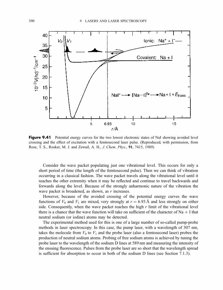
Consider the wave packet populating just one vibrational level. This occurs for only a
short period of time (the length of the femtosecond pulse). Then we can think of vibration
occurring in a classical fashion. The wave packet travels along the vibrational level until it
reaches the other extremity when it may be reflected and continue to travel backwards and
forwards along the level. Because of the strongly anharmonic nature of the vibration the
wave packet is broadened, as shown, as r increases.
However, because of the avoided crossing of the potential energy curves the wave
functions of V0 and V1 are mixed, very strongly at r ¼ 6.93 A and less strongly on either
side. Consequently, when the wave packet reaches the high r limit of the vibrational level
there is a chance that the wave function will take on sufficient of the character of Na þ I that
neutral sodium (or iodine) atoms may be detected.
The experimental method used for this is one of a large number of so-called pump-probe
methods in laser spectroscopy. In this case, the pump laser, with a wavelength of 307 nm,
takes the molecule from V0 to V1 and the probe laser (also a femtosecond laser) probes the
production of neutral sodium atoms. Probing of free sodium atoms is achieved by tuning the
probe laser to the wavelength of the sodium D lines at 589 nm and measuring the intensity of
the ensuing fluorescence. Pulses from the probe laser are so short that the wavelength spread
is sufficient for absorption to occur in both of the sodium D lines (see Section 7.1.3).
Figure 9.41 Potential energy curves for the two lowest electronic states of NaI showing avoided level
crossing and the effect of excitation with a femtosecond laser pulse. (Reproduced, with permission, from
Rose, T. S., Rosker, M. J. and Zewail, A. H., J. Chem. Phys., 91, 7415, 1989)
390 9 LASERS AND LASER SPECTROSCOPY
Figure 9.42(c) shows the result of measuring the intensity of sodium atom fluorescence at
589 nm as a function of time. This shows a steady increase from t ¼ 0 to a constant value
after about 7 ps but with some slight undulations in the region t ¼ 0–3 ps. The reason why
this curve does not level out more rapidly is that, because of the level crossing, the ‘ionic’
potential contains some of the character of the ‘covalent’ potential. Consequently, when the
wave packet reaches the high r end of the vibrational level it may be either reflected and
return to the t ¼ 0 position or escape into covalent territory. Therefore detection of neutral
free sodium atoms measures the rate of dissociation of excited NaI in the specific vibrational
energy level to which it was excited by the pump pulse. The small undulations in the signal
are caused by some of the wave packets being reflected and retained within the potential
well. The separation of the peaks is about 1.2 ps which is the time taken for the vibration to
occur.
Figure 9.42 Intensity of sodium atom fluorescence as a function of time following excitation of
NaI to the V1 potential with a pump wavelength of 307 nm (pulse duration ca 50 fs) and a probe
wavelength of (a) 575 nm, (b) 580 nm, (c) 589 nm, and (d) 615 nm. (Reproduced, with permission,
from Rose, T. S., Rosker, M. J. and Zewail, A. H., J. Chem. Phys., 91, 7415, 1989)
9.3 USES OF LASERS IN SPECTROSCOPY 391
Figures 9.42(a), 9.42(b) and 9.42(d) show the effect of keeping the pump wavelength
constant at 307 nm and varying the probe wavelength on either side of 589 nm. The most
remarkable feature of the resulting fluorescence signals is that they all show undulations
with the same peak separations as in Figure 9.42(c) but very much more prominently. Why
should fluorescence be observed when the probe wavelength is tuned away from the sodium
D lines? What is being observed is fluorescence from perturbed sodium atoms. These are
perturbed by the sodium atom still being lightly attached to the iodine atom in the transition
state and the very weakly bound Na � � � I being in an excited electronic state, (Na � � � I)*.Figures 9.42(a), 9.42(b) and 9.42(d), therefore, show the effect of (NaI)* having three
different, large internuclear distances. The prominent undulations, continuing for up to
about 8 ps, represent the probability of the wave packet being retained by being reflected
within the potential well.
Figure 9.41 shows that the potential curve for the excited state of NaI shows a shallow and
broad minimum. Such a potential shows vibrational levels which are strongly anharmonic
(see Section 6.1.3.2), closing up quickly with increasing vibrational quantum number.
Figure 9.43 shows the effect on the type of trace in Figures 9.42(a), 9.42(b) or 9.42(d) of
changing the pump wavelength and probing perturbed sodium atoms in the transition state.
As the pump wavelength decreases from (a) 300 nm to (b) 311 nm to (c) 321 nm to (d)
339 nm the quantum number of the vibrational level populated decreases. That the levels get
closer together, due to being highly anharmonic, is shown by the decrease in the period of
the undulations from about 1.5 to 1.0 ps. (The bottom of the well corresponds to about 400
nm.)
This general technique has been applied also to the direct observation of vibrational
motion in bound electronic states. Although no transition states as such are involved in
vibrational motion there is, again, a transitory change of internuclear distance.
An example of an investigation of vibrational motion in a bound (excited) electronic state
is in the B state of I2 (see Section 7.3.2). Figure 9.44 shows potential energy curves for three
electronic state of I2, the ground state X1Sþg , the first excited state B3P0þu and a higher
excited state f 0þg (a Hund’s case (c) state–see Section 7.2.2). Femtosecond wave packets
with a pump wavelength l1 (620 nm) excite the iodine molecules to a range of vibrational
levels in the B state corresponding to vertical transitions dictated by the Franck–Condon
principle. In this case the range is v ¼ 7–12 with a population distribution determined by the
intensity profile of the wave packet. Probing of the subsequent vibrational motion,
backwards and forwards along these levels, is achieved with a femtosecond pump laser of
wavelength l2. This takes the iodine molecules from the B state to vibrational levels of the f
state from which fluorescence, at a wavelength ldet, is detected.Figure 9.45(a) shows the resulting fluorescence intensity as a function of time. This is
dominated by oscillations with a period of about 300 fs but shows an amplitude modulation
with a period of about 10 ps. The 300 fs period is that of a vibration in the v ¼ 77 12 range
and the modulation is due to two neighbouring levels having slightly different frequencies
due to the vibration being anharmonic.
Figure 9.45(b) shows the result of Fourier transformation (see Section 3.3.3.2) of the
signal in Figure 9.45(a) from the time to the frequency domain. This transformation shows
clearly that two vibrations, with frequencies of about 3.3 THz (¼ 3.36 1012
392 9 LASERS AND LASER SPECTROSCOPY
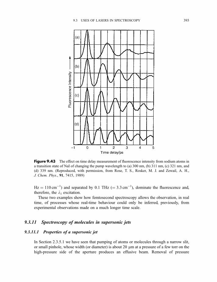
Hz ¼ 110 cm�1) and separated by 0.1 THz (¼ 3.3 cm�1), dominate the fluorescence and,
therefore, the l1 excitation.These two examples show how femtosecond spectroscopy allows the observation, in real
time, of processes whose real-time behaviour could only be inferred, previously, from
experimental observations made on a much longer time scale.
9.3.11 Spectroscopy of molecules in supersonic jets
9.3.11.1 Properties of a supersonic jet
In Section 2.3.5.1 we have seen that pumping of atoms or molecules through a narrow slit,
or small pinhole, whose width (or diameter) is about 20 mm at a pressure of a few torr on the
high-pressure side of the aperture produces an effusive beam. Removal of pressure
Figure 9.43 The effect on time delay measurement of fluorescence intensity from sodium atoms in
a transition state of NaI of changing the pump wavelength to (a) 300 nm, (b) 311 nm, (c) 321 nm, and
(d) 339 nm. (Reproduced, with permission, from Rose, T. S., Rosker, M. J. and Zewail, A. H.,
J. Chem. Phys., 91, 7415, 1989)
9.3 USES OF LASERS IN SPECTROSCOPY 393
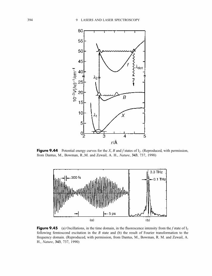
Figure 9.44 Potential energy curves for the X, B and f states of I2. (Reproduced, with permission,
from Dantus, M., Bowman, R.,M. and Zewail, A. H., Nature, 343, 737, 1990)
Figure 9.45 (a) Oscillations, in the time domain, in the fluorescence intensity from the f state of I2following femtoscond excitation in the B state and (b) the result of Fourier transformation to the
frequency domain. (Reproduced, with permission, from Dantus, M., Bowman, R. M. and Zewail, A.
H., Nature, 343, 737, 1990)
394 9 LASERS AND LASER SPECTROSCOPY
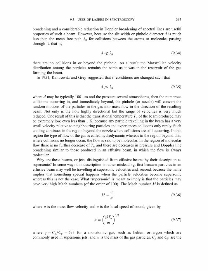
broadening and a considerable reduction in Doppler broadening of spectral lines are useful
properties of such a beam. However, because the slit width or pinhole diameter d is much
less than the mean free path l0 for collisions between the atoms or molecules passing
through it, that is,
d � l0 ð9:34Þ
there are no collisions in or beyond the pinhole. As a result the Maxwellian velocity
distribution among the particles remains the same as it was in the reservoir of the gas
forming the beam.
In 1951, Kantrowitz and Grey suggested that if conditions are changed such that
d l0 ð9:35Þ
where d may be typically 100 mm and the pressure several atmospheres, then the numerous
collisions occurring in, and immediately beyond, the pinhole (or nozzle) will convert the
random motions of the particles in the gas into mass flow in the direction of the resulting
beam. Not only is the flow highly directional but the range of velocities is very much
reduced. One result of this is that the translational temperature Ttr of the beam produced may
be extremely low, even less than 1 K, because any particle travelling in the beam has a very
small velocity relative to neighbouring particles and experiences collisions only rarely. Such
cooling continues in the region beyond the nozzle where collisions are still occurring. In this
region the type of flow of the gas is called hydrodynamic whereas in the region beyond this,
where collisions no longer occur, the flow is said to be molecular. In the region of molecular
flow there is no further decrease of Ttr and there are decreases in pressure and Doppler line
broadening similar to those produced in an effusive beam, in which the flow is always
molecular.
Why are these beams, or jets, distinguished from effusive beams by their description as
supersonic? In some ways this description is rather misleading, first because particles in an
effusive beam may well be travelling at supersonic velocities and, second, because the name
implies that something special happens when the particle velocities become supersonic
whereas this is not the case. What ‘supersonic’ is meant to imply is that the particles may
have very high Mach numbers (of the order of 100). The Mach number M is defined as
M ¼ u
að9:36Þ
where u is the mass flow velocity and a is the local speed of sound, given by
a ¼ gkTtrm
� �1=2
ð9:37Þ
where g ¼ Cp=CV ¼ 5=3 for a monatomic gas, such as helium or argon which are
commonly used in supersonic jets, and m is the mass of the gas particles. Cp and CV are the
9.3 USES OF LASERS IN SPECTROSCOPY 395
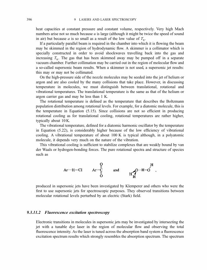
heat capacities at constant pressure and constant volume, respectively. Very high Mach
numbers arise not so much because u is large (although it might be twice the speed of sound
in air) but because a is so small as a result of the low value of Ttr.
If a particularly parallel beam is required in the chamber into which it is flowing the beam
may be skimmed in the region of hydrodynamic flow. A skimmer is a collimator which is
specially constructed in order to avoid shockwaves travelling back into the gas and
increasing Ttr. The gas that has been skimmed away may be pumped off in a separate
vacuum chamber. Further collimation may be carried out in the region of molecular flow and
a so-called supersonic beam results. When a skimmer is not used, a supersonic jet results:
this may or may not be collimated.
On the high-pressure side of the nozzle molecules may be seeded into the jet of helium or
argon and are also cooled by the many collisions that take place. However, in discussing
temperature in molecules, we must distinguish between translational, rotational and
vibrational temperatures. The translational temperature is the same as that of the helium or
argon carrier gas and may be less than 1 K.
The rotational temperature is defined as the temperature that describes the Boltzmann
population distribution among rotational levels. For example, for a diatomic molecule, this is
the temperature in Equation (5.15). Since collisions are not so efficient in producing
rotational cooling as for translational cooling, rotational temperatures are rather higher,
typically about 10K.
The vibrational temperature, defined for a diatomic harmonic oscillator by the temperature
in Equation (5.22), is considerably higher because of the low efficiency of vibrational
cooling. A vibrational temperature of about 100 K is typical although, in a polyatomic
molecule, it depends very much on the nature of the vibration.
This vibrational cooling is sufficient to stabilize complexes that are weakly bound by van
der Waals or hydrogen-bonding forces. The pure rotational spectra and structure of species
such as
produced in supersonic jets have been investigated by Klemperer and others who were the
first to use supersonic jets for spectroscopic purposes. They observed transitions between
molecular rotational levels perturbed by an electric (Stark) field.
9.3.11.2 Fluorescence excitation spectroscopy
Electronic transitions in molecules in supersonic jets may be investigated by intersecting the
jet with a tunable dye laser in the region of molecular flow and observing the total
fluorescence intensity. As the laser is tuned across the absorption band system a fluorescence
excitation spectrum results which strongly resembles the absorption spectrum. The spectrum
396 9 LASERS AND LASER SPECTROSCOPY
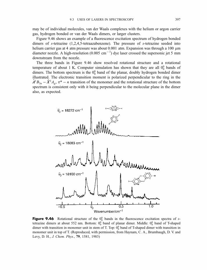
may be of individual molecules, van der Waals complexes with the helium or argon carrier
gas, hydrogen bonded or van der Waals dimers, or larger clusters.
Figure 9.46 shows an example of a fluorescence excitation spectrum of hydrogen bonded
dimers of s-tetrazine (1,2,4,5-tetraazabenzene). The pressure of s-tetrazine seeded into
helium carrier gas at 4 atm pressure was about 0.001 atm. Expansion was through a 100 mmdiameter nozzle. A high-resolution (0.005 cm71) dye laser crossed the supersonic jet 5 mm
downstream from the nozzle.
The three bands in Figure 9.46 show resolved rotational structure and a rotational
temperature of about 1 K. Computer simulation has shown that they are all 000 bands of
dimers. The bottom spectrum is the 000 band of the planar, doubly hydrogen bonded dimer
illustrated. The electronic transition moment is polarized perpendicular to the ring in the~AA1B3u � ~XX 1Ag, p*� n transition of the monomer and the rotational structure of the bottom
spectrum is consistent only with it being perpendicular to the molecular plane in the dimer
also, as expected.
Figure 9.46 Rotational structure of the 000 bands in the fluorescence excitation spectra of s-
tetrazine dimers at about 552 nm. Bottom: 000 band of planar dimer. Middle: 000 band of T-shaped
dimer with transition in monomer unit in stem of T. Top: 000 band of T-shaped dimer with transition in
monomer unit in top of T. (Reproduced, with permission, from Haynam, C. A., Brumbaugh, D. V. and
Levy, D. H., J. Chem. Phys., 79, 1581, 1983)
9.3 USES OF LASERS IN SPECTROSCOPY 397
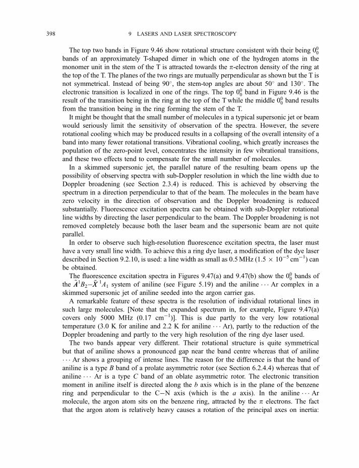
The top two bands in Figure 9.46 show rotational structure consistent with their being 000bands of an approximately T-shaped dimer in which one of the hydrogen atoms in the
monomer unit in the stem of the T is attracted towards the p-electron density of the ring at
the top of the T. The planes of the two rings are mutually perpendicular as shown but the T is
not symmetrical. Instead of being 90�, the stem-top angles are about 50� and 130�. Theelectronic transition is localized in one of the rings. The top 000 band in Figure 9.46 is the
result of the transition being in the ring at the top of the Twhile the middle 000 band results
from the transition being in the ring forming the stem of the T.
It might be thought that the small number of molecules in a typical supersonic jet or beam
would seriously limit the sensitivity of observation of the spectra. However, the severe
rotational cooling which may be produced results in a collapsing of the overall intensity of a
band into many fewer rotational transitions. Vibrational cooling, which greatly increases the
population of the zero-point level, concentrates the intensity in few vibrational transitions,
and these two effects tend to compensate for the small number of molecules.
In a skimmed supersonic jet, the parallel nature of the resulting beam opens up the
possibility of observing spectra with sub-Doppler resolution in which the line width due to
Doppler broadening (see Section 2.3.4) is reduced. This is achieved by observing the
spectrum in a direction perpendicular to that of the beam. The molecules in the beam have
zero velocity in the direction of observation and the Doppler broadening is reduced
substantially. Fluorescence excitation spectra can be obtained with sub-Doppler rotational
line widths by directing the laser perpendicular to the beam. The Doppler broadening is not
removed completely because both the laser beam and the supersonic beam are not quite
parallel.
In order to observe such high-resolution fluorescence excitation spectra, the laser must
have a very small line width. To achieve this a ring dye laser, a modification of the dye laser
described in Section 9.2.10, is used: a line width as small as 0.5MHz (1.56 10�5 cm�1) canbe obtained.
The fluorescence excitation spectra in Figures 9.47(a) and 9.47(b) show the 000 bands of
the ~AA1B2� ~XX 1A1 system of aniline (see Figure 5.19) and the aniline � � � Ar complex in a
skimmed supersonic jet of aniline seeded into the argon carrier gas.
A remarkable feature of these spectra is the resolution of individual rotational lines in
such large molecules. [Note that the expanded spectrum in, for example, Figure 9.47(a)
covers only 5000 MHz (0.17 cm�1)]. This is due partly to the very low rotational
temperature (3.0 K for aniline and 2.2 K for aniline � � � Ar), partly to the reduction of the
Doppler broadening and partly to the very high resolution of the ring dye laser used.
The two bands appear very different. Their rotational structure is quite symmetrical
but that of aniline shows a pronounced gap near the band centre whereas that of aniline
� � � Ar shows a grouping of intense lines. The reason for the difference is that the band of
aniline is a type B band of a prolate asymmetric rotor (see Section 6.2.4.4) whereas that of
aniline � � � Ar is a type C band of an oblate asymmetric rotor. The electronic transition
moment in aniline itself is directed along the b axis which is in the plane of the benzene
ring and perpendicular to the C�N axis (which is the a axis). In the aniline � � � Armolecule, the argon atom sits on the benzene ring, attracted by the p electrons. The fact
that the argon atom is relatively heavy causes a rotation of the principal axes on inertia:
398 9 LASERS AND LASER SPECTROSCOPY
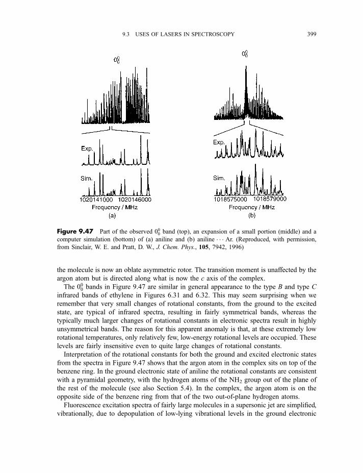
the molecule is now an oblate asymmetric rotor. The transition moment is unaffected by the
argon atom but is directed along what is now the c axis of the complex.
The 000 bands in Figure 9.47 are similar in general appearance to the type B and type C
infrared bands of ethylene in Figures 6.31 and 6.32. This may seem surprising when we
remember that very small changes of rotational constants, from the ground to the excited
state, are typical of infrared spectra, resulting in fairly symmetrical bands, whereas the
typically much larger changes of rotational constants in electronic spectra result in highly
unsymmetrical bands. The reason for this apparent anomaly is that, at these extremely low
rotational temperatures, only relatively few, low-energy rotational levels are occupied. These
levels are fairly insensitive even to quite large changes of rotational constants.
Interpretation of the rotational constants for both the ground and excited electronic states
from the spectra in Figure 9.47 shows that the argon atom in the complex sits on top of the
benzene ring. In the ground electronic state of aniline the rotational constants are consistent
with a pyramidal geometry, with the hydrogen atoms of the NH2 group out of the plane of
the rest of the molecule (see also Section 5.4). In the complex, the argon atom is on the
opposite side of the benzene ring from that of the two out-of-plane hydrogen atoms.
Fluorescence excitation spectra of fairly large molecules in a supersonic jet are simplified,
vibrationally, due to depopulation of low-lying vibrational levels in the ground electronic
Figure 9.47 Part of the observed 000 band (top), an expansion of a small portion (middle) and a
computer simulation (bottom) of (a) aniline and (b) aniline � � � Ar. (Reproduced, with permission,
from Sinclair, W. E. and Pratt, D. W., J. Chem. Phys., 105, 7942, 1996)
9.3 USES OF LASERS IN SPECTROSCOPY 399
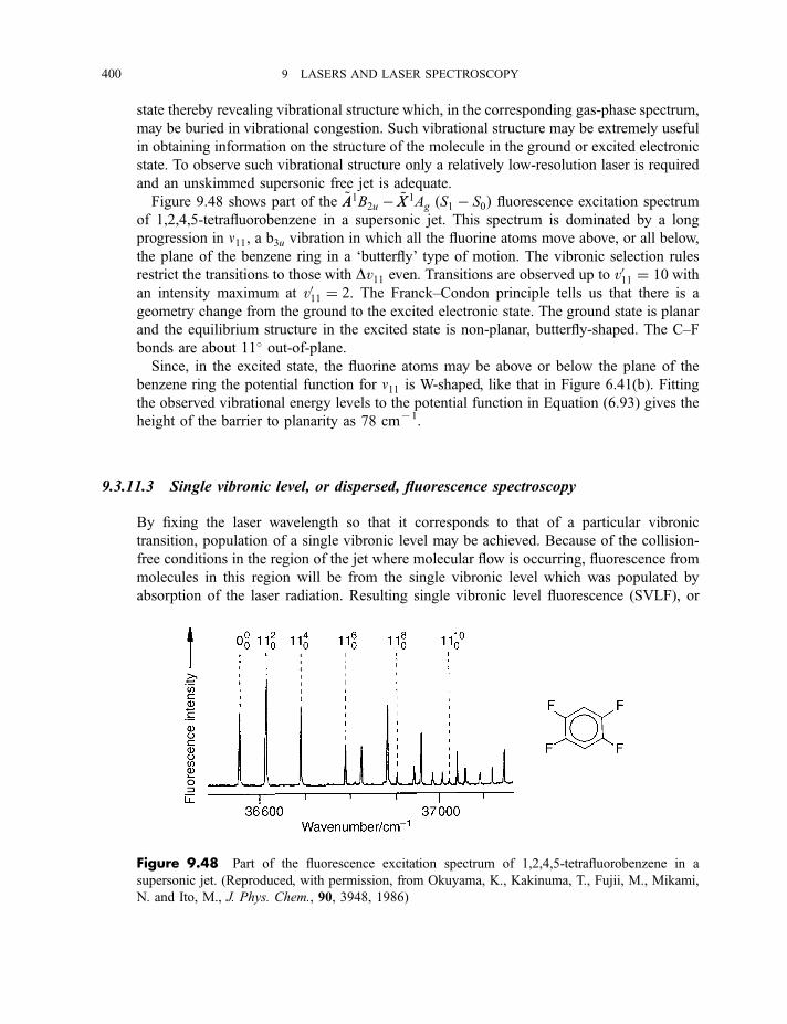
state thereby revealing vibrational structure which, in the corresponding gas-phase spectrum,
may be buried in vibrational congestion. Such vibrational structure may be extremely useful
in obtaining information on the structure of the molecule in the ground or excited electronic
state. To observe such vibrational structure only a relatively low-resolution laser is required
and an unskimmed supersonic free jet is adequate.
Figure 9.48 shows part of the ~AA1B2u � ~XX 1Ag ðS1 � S0Þ fluorescence excitation spectrum
of 1,2,4,5-tetrafluorobenzene in a supersonic jet. This spectrum is dominated by a long
progression in n11, a b3u vibration in which all the fluorine atoms move above, or all below,
the plane of the benzene ring in a ‘butterfly’ type of motion. The vibronic selection rules
restrict the transitions to those with Dv11 even. Transitions are observed up to v011 ¼ 10 with
an intensity maximum at v011 ¼ 2. The Franck–Condon principle tells us that there is a
geometry change from the ground to the excited electronic state. The ground state is planar
and the equilibrium structure in the excited state is non-planar, butterfly-shaped. The C–F
bonds are about 11� out-of-plane.Since, in the excited state, the fluorine atoms may be above or below the plane of the
benzene ring the potential function for n11 is W-shaped, like that in Figure 6.41(b). Fitting
the observed vibrational energy levels to the potential function in Equation (6.93) gives the
height of the barrier to planarity as 78 cm71.
9.3.11.3 Single vibronic level, or dispersed, fluorescence spectroscopy
By fixing the laser wavelength so that it corresponds to that of a particular vibronic
transition, population of a single vibronic level may be achieved. Because of the collision-
free conditions in the region of the jet where molecular flow is occurring, fluorescence from
molecules in this region will be from the single vibronic level which was populated by
absorption of the laser radiation. Resulting single vibronic level fluorescence (SVLF), or
Figure 9.48 Part of the fluorescence excitation spectrum of 1,2,4,5-tetrafluorobenzene in a
supersonic jet. (Reproduced, with permission, from Okuyama, K., Kakinuma, T., Fujii, M., Mikami,
N. and Ito, M., J. Phys. Chem., 90, 3948, 1986)
400 9 LASERS AND LASER SPECTROSCOPY
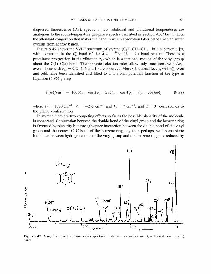
dispersed fluorescence (DF), spectra at low rotational and vibrational temperatures are
analogous to the room-temperature gas-phase spectra described in Section 9.3.7 but without
the attendant congestion that makes the band in which absorption takes place likely to suffer
overlap from nearby bands.
Figure 9.49 shows the SVLF spectrum of styrene (C6H5CH¼CH2), in a supersonic jet,
with excitation in the 000 band of the ~AA1A0 � ~XX 1A0 ðS1 � S0Þ band system. There is a
prominent progression in the vibration n42 which is a torsional motion of the vinyl group
about the C(1)–C(a) bond. The vibronic selection rules allow only transitions with Dv42even. Those with v0042 ¼ 0, 2, 4, 6 and 10 are observed. More vibrational levels, with v0042 evenand odd, have been identified and fitted to a torsional potential function of the type in
Equation (6.96) giving
V ðfÞ=cm�1 ¼ ½1070ð1� cos 2fÞ � 275ð1� cos 4fÞ þ 7ð1� cos 6fÞ� ð9:38Þ
where V2 ¼ 1070 cm�1, V4 ¼ �275 cm�1 and V6 ¼ 7 cm�1; and f ¼ 0� corresponds to
the planar configuration.
In styrene there are two competing effects so far as the possible planarity of the molecule
is concerned. Conjugation between the double bond of the vinyl group and the benzene ring
is favoured by planarity but through-space interaction between the double bond of the vinyl
group and the nearest C–C bond of the benzene ring, together, perhaps, with some steric
hindrance between hydrogen atoms of the vinyl group and the benzene ring, are reduced by
Figure 9.49 Single vibronic level fluorescence spectrum of styrene, in a supersonic jet, with excitation in the 000band
9.3 USES OF LASERS IN SPECTROSCOPY 401
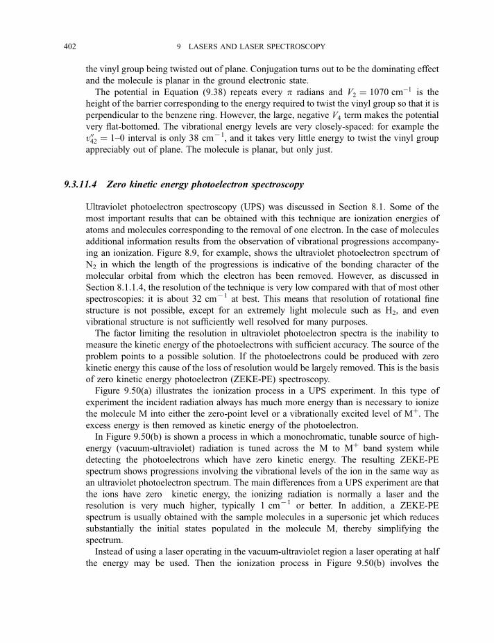
the vinyl group being twisted out of plane. Conjugation turns out to be the dominating effect
and the molecule is planar in the ground electronic state.
The potential in Equation (9.38) repeats every p radians and V2 ¼ 1070 cm�1 is the
height of the barrier corresponding to the energy required to twist the vinyl group so that it is
perpendicular to the benzene ring. However, the large, negative V4 term makes the potential
very flat-bottomed. The vibrational energy levels are very closely-spaced: for example the
v0042 ¼ 1–0 interval is only 38 cm71, and it takes very little energy to twist the vinyl group
appreciably out of plane. The molecule is planar, but only just.
9.3.11.4 Zero kinetic energy photoelectron spectroscopy
Ultraviolet photoelectron spectroscopy (UPS) was discussed in Section 8.1. Some of the
most important results that can be obtained with this technique are ionization energies of
atoms and molecules corresponding to the removal of one electron. In the case of molecules
additional information results from the observation of vibrational progressions accompany-
ing an ionization. Figure 8.9, for example, shows the ultraviolet photoelectron spectrum of
N2 in which the length of the progressions is indicative of the bonding character of the
molecular orbital from which the electron has been removed. However, as discussed in
Section 8.1.1.4, the resolution of the technique is very low compared with that of most other
spectroscopies: it is about 32 cm71 at best. This means that resolution of rotational fine
structure is not possible, except for an extremely light molecule such as H2, and even
vibrational structure is not sufficiently well resolved for many purposes.
The factor limiting the resolution in ultraviolet photoelectron spectra is the inability to
measure the kinetic energy of the photoelectrons with sufficient accuracy. The source of the
problem points to a possible solution. If the photoelectrons could be produced with zero
kinetic energy this cause of the loss of resolution would be largely removed. This is the basis
of zero kinetic energy photoelectron (ZEKE-PE) spectroscopy.
Figure 9.50(a) illustrates the ionization process in a UPS experiment. In this type of
experiment the incident radiation always has much more energy than is necessary to ionize
the molecule M into either the zero-point level or a vibrationally excited level of Mþ. Theexcess energy is then removed as kinetic energy of the photoelectron.
In Figure 9.50(b) is shown a process in which a monochromatic, tunable source of high-
energy (vacuum-ultraviolet) radiation is tuned across the M to Mþ band system while
detecting the photoelectrons which have zero kinetic energy. The resulting ZEKE-PE
spectrum shows progressions involving the vibrational levels of the ion in the same way as
an ultraviolet photoelectron spectrum. The main differences from a UPS experiment are that
the ions have zero kinetic energy, the ionizing radiation is normally a laser and the
resolution is very much higher, typically 1 cm71 or better. In addition, a ZEKE-PE
spectrum is usually obtained with the sample molecules in a supersonic jet which reduces
substantially the initial states populated in the molecule M, thereby simplifying the
spectrum.
Instead of using a laser operating in the vacuum-ultraviolet region a laser operating at half
the energy may be used. Then the ionization process in Figure 9.50(b) involves the
402 9 LASERS AND LASER SPECTROSCOPY
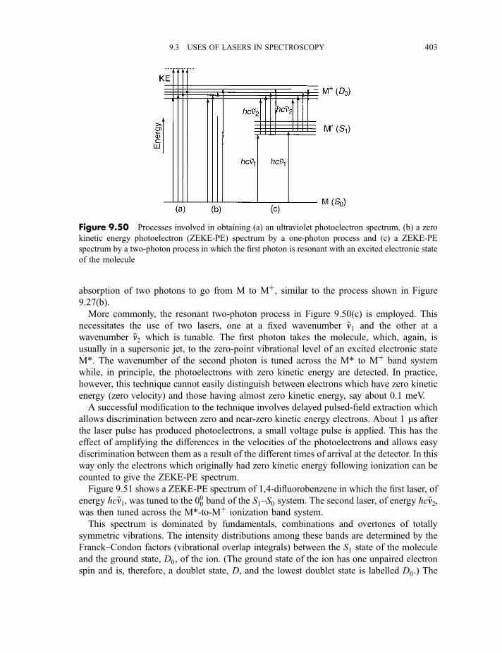
absorption of two photons to go from M to Mþ, similar to the process shown in Figure
9.27(b).
More commonly, the resonant two-photon process in Figure 9.50(c) is employed. This
necessitates the use of two lasers, one at a fixed wavenumber ~nn1 and the other at a
wavenumber ~nn2 which is tunable. The first photon takes the molecule, which, again, is
usually in a supersonic jet, to the zero-point vibrational level of an excited electronic state
M*. The wavenumber of the second photon is tuned across the M* to Mþ band system
while, in principle, the photoelectrons with zero kinetic energy are detected. In practice,
however, this technique cannot easily distinguish between electrons which have zero kinetic
energy (zero velocity) and those having almost zero kinetic energy, say about 0.1 meV.
A successful modification to the technique involves delayed pulsed-field extraction which
allows discrimination between zero and near-zero kinetic energy electrons. About 1 ms afterthe laser pulse has produced photoelectrons, a small voltage pulse is applied. This has the
effect of amplifying the differences in the velocities of the photoelectrons and allows easy
discrimination between them as a result of the different times of arrival at the detector. In this
way only the electrons which originally had zero kinetic energy following ionization can be
counted to give the ZEKE-PE spectrum.
Figure 9.51 shows a ZEKE-PE spectrum of 1,4-difluorobenzene in which the first laser, of
energy hc~nn1, was tuned to the 000 band of the S1–S0 system. The second laser, of energy hc~nn2,was then tuned across the M*-to-Mþ ionization band system.
This spectrum is dominated by fundamentals, combinations and overtones of totally
symmetric vibrations. The intensity distributions among these bands are determined by the
Franck–Condon factors (vibrational overlap integrals) between the S1 state of the molecule
and the ground state, D0, of the ion. (The ground state of the ion has one unpaired electron
spin and is, therefore, a doublet state, D, and the lowest doublet state is labelled D0.) The
Figure 9.50 Processes involved in obtaining (a) an ultraviolet photoelectron spectrum, (b) a zero
kinetic energy photoelectron (ZEKE-PE) spectrum by a one-photon process and (c) a ZEKE-PE
spectrum by a two-photon process in which the first photon is resonant with an excited electronic state
of the molecule
9.3 USES OF LASERS IN SPECTROSCOPY 403
fact that the intensity of the 000 band is very dominant indicates that there is no substantial
geometry change in going from the S1 state of the molecule to the D0 state of the cation.
The resolution of the ZEKE-PE spectrum of 1,4-difluorobenzene can be compared with,
for example, that of the ultraviolet photoelectron spectrum of benzene in Figure 8.12. The
greatly increased resolution in the ZEKE-PE spectrum is attributable mostly to the fact that
only photoelectrons with zero kinetic energy are being detected. It is also partly attributable
to the molecules being in a supersonic jet; this has the effect of sharpening the bands
because of the restricted rotational populations in the ground state of the molecule.
The ZEKE-PE process shown in Figure 9.50(c) can be modified as shown by changing the
wavenumber ~nn1 of the first laser to excite the molecule to an excited vibrational level of M*.
Then the Franck–Condon factors for the D0–S1 band system are modified. This can allow
access to more vibrational levels of the cation than is possible with initial excitation in the 000band of the S1–S0 system.
Exercises
9.1 Show that the 10.6 mm and 9.6 mm radiation from a CO2 laser is due to transitions
allowed by electric dipole selection rules.
9.2 Draw a diagram similar to that in Figure 9.21 to illustrate the stimulated Raman effect
in H2. High-pressure H2 is used to Raman shift radiation from a KrF laser. Calculate
the two wavelengths of the shifted radiation which are closest to that of the KrF laser.
Figure 9.51 A zero kinetic energy photoelectron (ZEKE-PE) resonant two-photon spectrum of
1,4-difluorobenzene in which the first photon excites the molecule of the zero-point level of the S1excited electronic state of the molecule. (Reproduced, with permission, from Reiser, G., Rieger, D.,
Wright, T.G., Muller-Dethlefs, K. and Schlag, E.W., J. Phys. Chem., 97, 4335, 1993)
404 9 LASERS AND LASER SPECTROSCOPY

9.3 Write down the symmetry species of vibrations which are allowed in the CARS
spectrum of CH4.
9.4 In the two-photon spectrum in Figure 9.29 the vibrations n18a,n17b, n16a and n15 have
symmetry species b1u, b3u, au and b2u, respectively. Show that the 18a10, 17b10, 16a
10 and
1510 transitions are allowed by symmetry.
9.5 In a cavity ring-down absorption experiment the length of the cavity is 1.24m. What is
the time interval between the detected signals?
9.6 Unlike the situation regarding the crossing between the V0 and V1 potentials for NaI
(see Figure 9.41), that for NaBr results in very efficient and rapid dissociation to give
Naþ Br when it is excited to V1. How would you expect the fluorescence intensity
from the neutral bromine atoms to vary with time compared with that for iodine atoms
from NaI in Figure 9.42?
Bibliography
Andrews, D. L. (1997) Lasers in Chemistry, 2nd edn, Springer-Verlag, Berlin.
Beesley, M. J. (1971) Lasers and their Applications, Taylor and Francis, London.
Demtroder, W. (1996) Laser Spectroscopy, 2nd edn, Springer, Berlin.
Lengyel, B. A. (1971) Lasers, Wiley-Interscience, New York.
Siegman, A. E. (1986) Lasers, University Science Books, Sausalito.
Silfvast, W. T. (1996) Laser Fundamentals, Cambridge University Press, Cambridge.
Svelto, O. (1998) Principles of Lasers, 2nd edn, Kluwer, Dordrecht.
Zewail, A. H. (1994) Femtochemistry, World Scientific Publishing, New Jersey.
BIBLIOGRAPHY 405

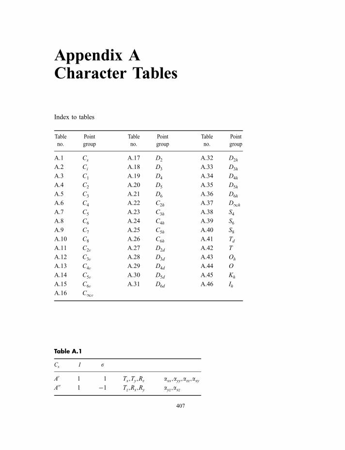
Appendix ACharacter Tables
Index to tables
Table
no.
Point
group
Table
no.
Point
group
Table
no.
Point
group
A.1 Cs A.17 D2 A.32 D2h
A.2 Ci A.18 D3 A.33 D3h
A.3 C1 A.19 D4 A.34 D4h
A.4 C2 A.20 D5 A.35 D5h
A.5 C3 A.21 D6 A.36 D6h
A.6 C4 A.22 C2h A.37 D1h
A.7 C5 A.23 C3h A.38 S4
A.8 C6 A.24 C4h A.39 S6
A.9 C7 A.25 C5h A.40 S8
A.10 C8 A.26 C6h A.41 Td
A.11 C2v A.27 D2d A.42 T
A.12 C3v A.28 D3d A.43 Oh
A.13 C4v A.29 D4d A.44 O
A.14 C5v A.30 D5d A.45 Kh
A.15 C6v A.31 D6d A.46 Ih
A.16 C1v
Table A.1
Cs I s
A0 1 1 Tx;Ty;Rz axx;ayy;azz;axyA00 1 �1 Tz;Rx;Ry ayz;axz
407
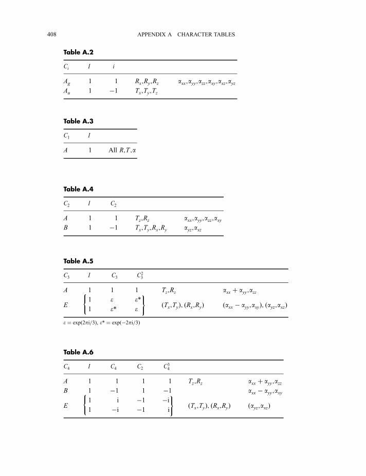
Table A.2
Ci I i
Ag 1 1 Rx;Ry;Rz axx;ayy;azz;axy;axz;ayzAu 1 �1 Tx;Ty;Tz
Table A.3
C1 I
A 1 All R;T ;a
Table A.4
C2 I C2
A 1 1 Tz;Rz axx;ayy;azz;axyB 1 �1 Tx;Ty;Rx;Ry ayz;axz
Table A.5
C3 I C3 C23
A 1 1 1 Tz;Rz axx þ ayy;azz
E
(1 e e*
)ðTx;TyÞ; ðRx;RyÞ ðaxx � ayy;axyÞ; ðayz;axzÞ1 e* e
e ¼ expð2pi=3Þ, e* ¼ expð�2pi=3Þ
Table A.6
C4 I C4 C2 C34
A 1 1 1 1 Tz;Rz axx þ ayy;azzB 1 �1 1 �1 axx � ayy;axy
E
(1 i �1 �i
)ðTx;TyÞ; ðRx;RyÞ ðayz;axzÞ1 �i �1 i
408 APPENDIX A CHARACTER TABLES
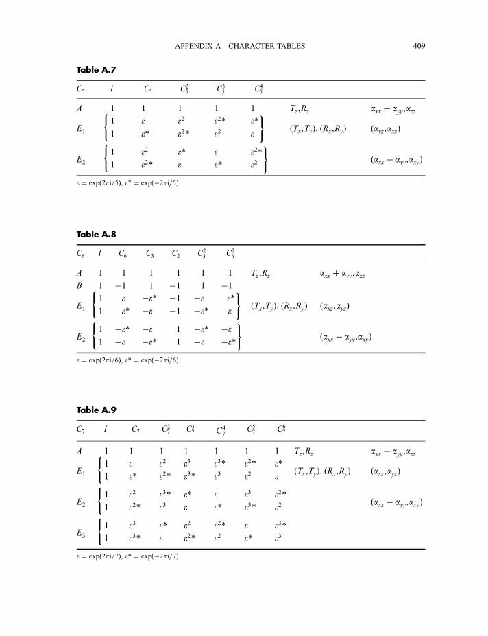
Table A.7
C5 I C5 C25 C3
5 C45
A 1 1 1 1 1 Tz;Rz axx þ ayy;azz
E1
(1 e e2 e2* e*
)ðTx;TyÞ; ðRx;RyÞ ðayz;axzÞ1 e* e2* e2 e
E2
(1 e2 e* e e2*
)ðaxx � ayy;axyÞ1 e2* e e* e2
e ¼ expð2pi=5Þ, e* ¼ expð�2pi=5Þ
Table A.8
C6 I C6 C3 C2 C23 C5
6
A 1 1 1 1 1 1 Tz;Rz axx þ ayy;azzB 1 �1 1 �1 1 �1
E1
(1 e �e* �1 �e e*
)ðTx;TyÞ; ðRx;RyÞ ðaxz;ayzÞ1 e* �e �1 �e* e
E2
(1 �e* �e 1 �e* �e
)ðaxx � ayy;axyÞ1 �e �e* 1 �e �e*
e ¼ expð2pi=6Þ, e* ¼ expð�2pi=6Þ
Table A.9
C7 I C7 C27 C3
7 C47
C57 C6
7
A 1 1 1 1 1 1 1 Tz;Rz axx þ ayy;azz
E1
(1 e e2 e3 e3* e2* e* ðTx;TyÞ; ðRx;RyÞ ðaxz;ayzÞ1 e* e2* e3* e3 e2 e
E2
(1 e2 e3* e* e e3 e2* ðaxx � ayy;axyÞ1 e2* e3 e e* e3* e2
E3
(1 e3 e* e2 e2* e e3*1 e3* e e2* e2 e* e3
e ¼ expð2pi=7Þ, e* ¼ expð�2pi=7Þ
APPENDIX A CHARACTER TABLES 409
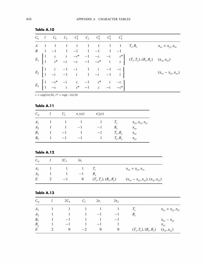
Table A.10
C8 I C8 C4 C38 C2 C5
8 C34 C7
8
A 1 1 1 1 1 1 1 1 Tz;Rz axx þ ayy;azzB 1 �1 1 �1 1 �1 1 �1
E1
(1 e i �e* �1 �e �i e*
)ðTx;TyÞ; ðRx;RyÞ ðaxz;ayzÞ1 e* �i �e �1 �e* i e
E2
(1 i �1 �i 1 i �1 �i
)ðaxx � ayy;axyÞ1 �i �1 i 1 �i �1 i
E3
(1 �e* �i e �1 e* i �e
)1 �e i e* �1 e �i �e*
e ¼ expð2pi=8Þ, e* ¼ expð�2pi=8Þ
Table A.11
C2v I C2 sv ðxzÞ s0vðyzÞ
A1 1 1 1 1 Tz axx;ayy;azzA2 1 1 �1 �1 Rz axyB1 1 �1 1 �1 Tx;Ry axzB2 1 �1 �1 1 Ty;Rx ayz
Table A.12
C3v I 2C3 3sv
A1 1 1 1 Tz axx þ ayy;azzA2 1 1 �1 Rz
E 2 �1 0 ðTx;TyÞ; ðRx;RyÞ ðaxx � ayy;axyÞ; ðaxz;ayzÞ
Table A.13
C4v I 2C4 C2 2sv 2sd
A1 1 1 1 1 1 Tz axx þ ayy;azzA2 1 1 1 �1 �1 Rz
B1 1 �1 1 1 �1 axx � ayyB2
1 �1 1 �1 1 axyE 2 0 �2 0 0 ðTx;TyÞ; ðRx;RyÞ ðaxz;ayzÞ
410 APPENDIX A CHARACTER TABLES
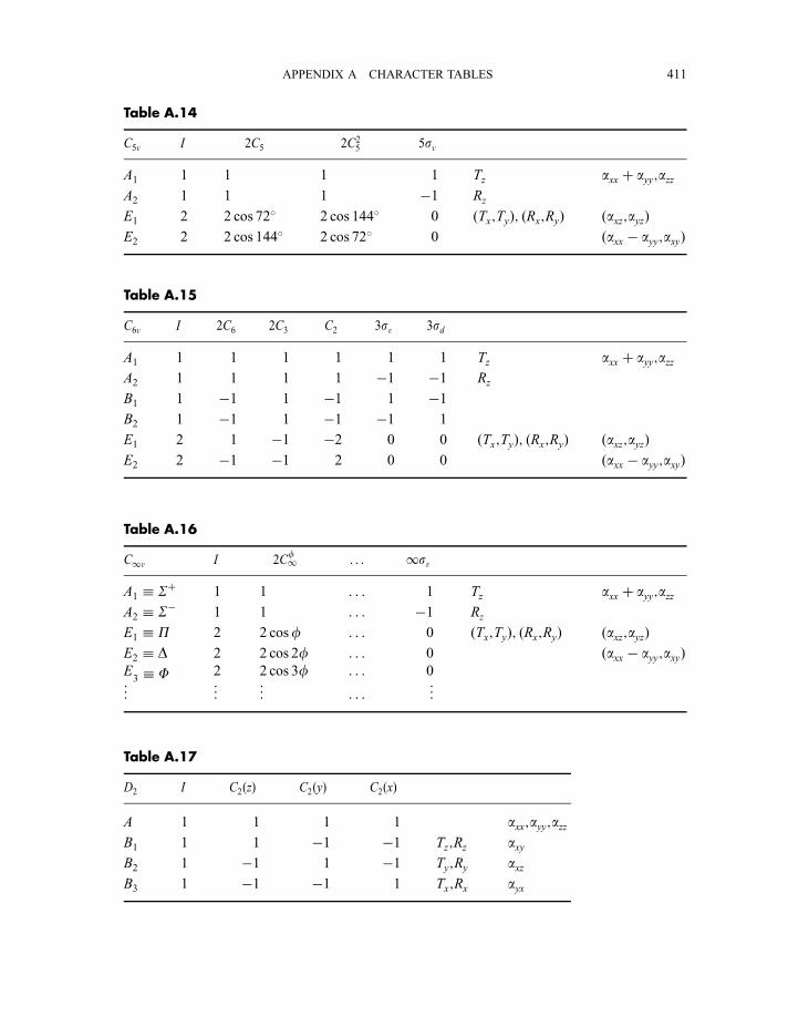
Table A.14
C5v I 2C5 2C25 5sv
A1 1 1 1 1 Tz axx þ ayy;azzA2 1 1 1 �1 Rz
E1 2 2 cos 72� 2 cos 144� 0 ðTx;TyÞ; ðRx;RyÞ ðaxz;ayzÞE2 2 2 cos 144� 2 cos 72� 0 ðaxx � ayy;axyÞ
Table A.15
C6v I 2C6 2C3 C2 3sv 3sd
A1 1 1 1 1 1 1 Tz axx þ ayy;azzA2 1 1 1 1 �1 �1 Rz
B1 1 �1 1 �1 1 �1B2 1 �1 1 �1 �1 1
E1 2 1 �1 �2 0 0 ðTx;TyÞ; ðRx;RyÞ ðaxz;ayzÞE2 2 �1 �1 2 0 0 ðaxx � ayy;axyÞ
Table A.16
C1v I 2Cf1 . . . 1sv
A1 Sþ 1 1 . . . 1 Tz axx þ ayy;azzA2 S� 1 1 . . . �1 Rz
E1 P 2 2 cosf . . . 0 ðTx;TyÞ; ðRx;RyÞ ðaxz;ayzÞE2 D 2 2 cos 2f . . . 0 ðaxx � ayy;axyÞE3 F 2 2 cos 3f . . . 0
..
. ... ..
.. . . ..
.
Table A.17
D2 I C2ðzÞ C2ðyÞ C2ðxÞ
A 1 1 1 1 axx;ayy;azzB1 1 1 �1 �1 Tz;Rz axyB2 1 �1 1 �1 Ty;Ry axzB3 1 �1 �1 1 Tx;Rx ayx
APPENDIX A CHARACTER TABLES 411
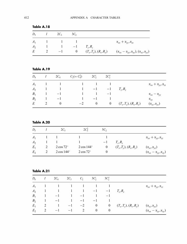
Table A.18
D3 I 2C3 3C2
A1 1 1 1 axx þ ayy;azzA2 1 1 �1 Tz;Rz
E 2 �1 0 ðTx;TyÞ; ðRx;RyÞ ðaxx � ayy;axyÞ; ðaxz;ayzÞ
Table A.19
D4 I 2C4 C2ð¼ C24 Þ 2C02 2C002
A1 1 1 1 1 1 axx þ ayy;azzA2 1 1 1 �1 �1 Tz;Rz
B1 1 �1 1 1 �1 axx � ayyB2 1 �1 1 �1 1 axyE 2 0 �2 0 0 ðTx;TyÞ; ðRx;RyÞ ðaxz;ayzÞ
Table A.20
D5 I 2C5 2C25 5C2
A1 1 1 1 1 axx þ ayy;azzA2 1 1 1 �1 Tz;Rz
E1 2 2 cos 72� 2 cos 144� 0 ðTx;TyÞ; ðRx;RyÞ ðaxz;ayzÞE2 2 2 cos 144� 2 cos 72� 0 ðaxx � ayy;axyÞ
Table A.21
D6 I 2C6 2C3 C2 3C02 3C002
A1 1 1 1 1 1 1 axx þ ayy;azzA2 1 1 1 1 �1 �1 Tz;Rz
B1 1 �1 1 �1 1 �1B2 1 �1 1 �1 �1 1
E1 2 1 �1 �2 0 0 ðTx;TyÞ; ðRx;RyÞ ðaxz;ayzÞE2 2 �1 �1 2 0 0 ðaxx � ayy;axyÞ
412 APPENDIX A CHARACTER TABLES
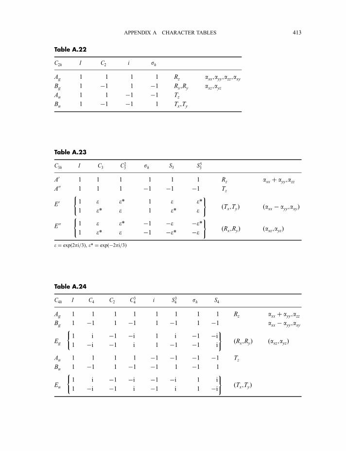
Table A.22
C2h I C2 i sh
Ag 1 1 1 1 Rz axx;ayy;azz;axyBg 1 �1 1 �1 Rx;Ry axz;ayzAu 1 1 �1 �1 Tz
Bu 1 �1 �1 1 Tx;Ty
Table A.23
C3h I C3 C23 sh S3 S53
A0 1 1 1 1 1 1 Rz axx þ ayy;azzA00 1 1 1 �1 �1 �1 Tz
E0(1 e e* 1 e e*
)ðTx;TyÞ ðaxx � ayy;axyÞ1 e* e 1 e* e
E00(1 e e* �1 �e �e*
)ðRx;RyÞ ðaxz;ayzÞ1 e* e �1 �e* �e
e ¼ expð2pi=3Þ, e* ¼ expð�2pi=3Þ
Table A.24
C4h I C4 C2 C34 i S34 sh S4
Ag 1 1 1 1 1 1 1 1 Rz axx þ ayy;azzBg 1 �1 1 �1 1 �1 1 �1 axx � ayy;axy
Eg
(1 i �1 �i 1 i �1 �i
)ðRx;RyÞ ðaxz;ayzÞ1 �i �1 i 1 �1 �1 i
Au 1 1 1 1 �1 �1 �1 �1 Tz
Bu 1 �1 1 �1 �1 1 �1 1
Eu
(1 i �1 �i �1 �i 1 i
)ðTx;TyÞ1 �i �1 i �1 i 1 �i
APPENDIX A CHARACTER TABLES 413
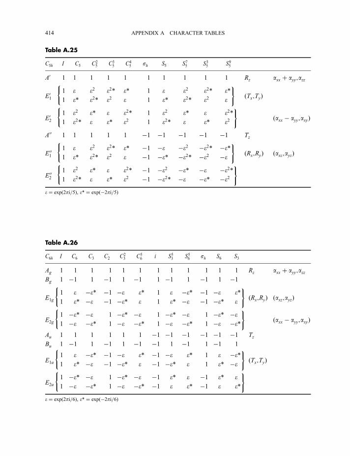
Table A.25
C5h I C5 C25 C3
5 C45 sh S5 S75 S35 S95
A0 1 1 1 1 1 1 1 1 1 1 Rz axx þ ayy;azz
E01
(1 e e2 e2* e* 1 e e2 e2* e*
)ðTx;TyÞ1 e* e2* e2 e 1 e* e2* e2 e
E02
(1 e2 e* e e2* 1 e2 e* e e2*
)ðaxx � ayy;axyÞ1 e2* e e* e2 1 e2* e e* e2
A00 1 1 1 1 1 �1 �1 �1 �1 �1 Tz
E001
(1 e e2 e2* e* �1 �e �e2 �e2* �e*
)ðRx;RyÞ ðaxz;ayzÞ1 e* e2* e2 e �1 �e* �e2* �e2 �e
E002
(1 e2 e* e e2* �1 �e2 �e* �e �e2*
)1 e2* e e* e2 �1 �e2* �e �e* �e2
e ¼ expð2pi=5Þ, e* ¼ expð�2pi=5Þ
Table A.26
C6h I C6 C3 C2 C23 C5
6 i S53 S56 sh S6 S3
Ag 1 1 1 1 1 1 1 1 1 1 1 1 Rz axx þ ayy;azzBg 1 �1 1 �1 1 �1 1 �1 1 �1 1 �1
E1g
(1 e �e* �1 �e e* 1 e �e* �1 �e e*
)ðRx;RyÞ ðaxz;ayzÞ1 e* �e �1 �e* e 1 e* �e �1 �e* e
E2g
(1 �e* �e 1 �e* �e 1 �e* �e 1 �e* �e
)ðaxx � ayy;axyÞ1 �e �e* 1 �e �e* 1 �e �e* 1 �e �e*
Au 1 1 1 1 1 1 �1 �1 �1 �1 �1 �1 Tz
Bu 1 �1 1 �1 1 �1 �1 1 �1 1 �1 1
E1u
(1 e �e* �1 �e e* �1 �e e* 1 e �e*
)ðTx;TyÞ1 e* �e �1 �e* e �1 �e* e 1 e* �e
E2u
(1 �e* �e 1 �e* �e �1 e* e �1 e* e
)1 �e �e* 1 �e �e* �1 e e* �1 e e*
e ¼ expð2pi=6Þ, e* ¼ expð�2pi=6Þ
414 APPENDIX A CHARACTER TABLES
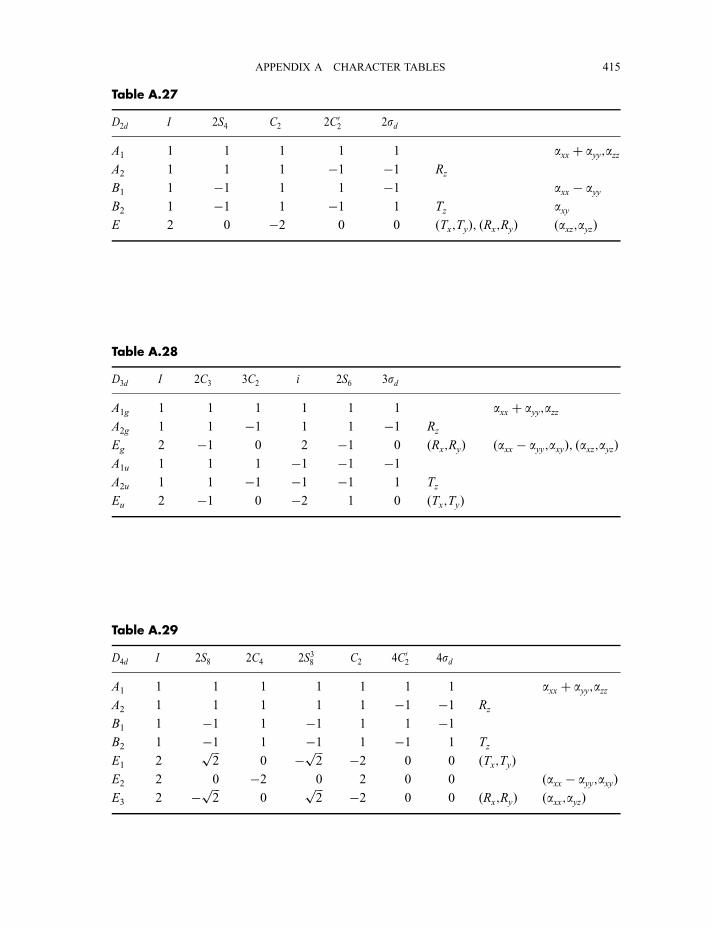
Table A.27
D2d I 2S4 C2 2C02 2sd
A1 1 1 1 1 1 axx þ ayy;azzA2 1 1 1 �1 �1 Rz
B1 1 �1 1 1 �1 axx � ayyB2 1 �1 1 �1 1 Tz axyE 2 0 �2 0 0 ðTx;TyÞ; ðRx;RyÞ ðaxz;ayzÞ
Table A.28
D3d I 2C3 3C2 i 2S6 3sd
A1g 1 1 1 1 1 1 axx þ ayy;azzA2g 1 1 �1 1 1 �1 Rz
Eg 2 �1 0 2 �1 0 ðRx;RyÞ ðaxx � ayy;axyÞ; ðaxz;ayzÞA1u 1 1 1 �1 �1 �1A2u 1 1 �1 �1 �1 1 Tz
Eu 2 �1 0 �2 1 0 ðTx;TyÞ
Table A.29
D4d I 2S8 2C4 2S38 C2 4C02 4sd
A1 1 1 1 1 1 1 1 axx þ ayy;azzA2 1 1 1 1 1 �1 �1 Rz
B1 1 �1 1 �1 1 1 �1B2 1 �1 1 �1 1 �1 1 Tz
E1 2ffiffiffi2p
0 � ffiffiffi2p �2 0 0 ðTx;TyÞ
E2 2 0 �2 0 2 0 0 ðaxx � ayy;axyÞE3 2 � ffiffiffi
2p
0ffiffiffi2p �2 0 0 ðRx;RyÞ ðaxx;ayzÞ
APPENDIX A CHARACTER TABLES 415
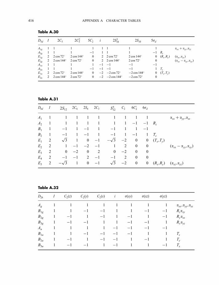
Table A.31
D6d I 2S12 2C6 2S4 2C3 S512C2 6C02 6sd
A1 1 1 1 1 1 1 1 1 1 axx þ ayy;azzA2 1 1 1 1 1 1 1 �1 �1 Rz
B1 1 �1 1 �1 1 �1 1 1 �1B2 1 �1 1 �1 1 �1 1 �1 1 Tz
E1 2ffiffiffi3p
1 0 �1 � ffiffiffi3p �2 0 0 ðTx;TyÞ
E2 2 1 �1 �2 �1 1 2 0 0 ðaxx � ayy;axyÞE3 2 0 �2 0 2 0 �2 0 0
E4 2 �1 �1 2 �1 �1 2 0 0
E5 2 � ffiffiffi3p
1 0 �1 ffiffiffi3p �2 0 0 ðRx;RyÞ ðaxz;ayzÞ
Table A.32
D2h I C2ðzÞ C2ðyÞ C2ðxÞ i sðxyÞ sðxzÞ sðyzÞ
Ag 1 1 1 1 1 1 1 1 axx;ayy;azzB1g 1 1 �1 �1 1 1 �1 �1 RzaxyB2g 1 �1 1 �1 1 �1 1 �1 RyaxzB3g 1 �1 �1 1 1 �1 �1 1 RxayzAu 1 1 1 1 �1 �1 �1 �1B1u 1 1 �1 �1 �1 �1 1 1 Tz
B2u 1 �1 1 �1 �1 1 �1 1 Ty
B3u 1 �1 �1 1 �1 1 1 �1 Tx
Table A.30
D5d I 2C5 2C25 5C2 i 2S310 2S10 5sd
A1g 1 1 1 1 1 1 1 1 axx þ ayy;azzA2g 1 1 1 �1 1 1 1 �1 Rz
E1g 2 2 cos 72� 2 cos 144� 0 2 2 cos 72� 2 cos 144� 0 ðRx;RyÞ ðaxz;ayzÞE2g 2 2 cos 144� 2 cos 72� 0 2 2 cos 144� 2 cos 72� 0 ðaxx � ayy;axyÞA1u 1 1 1 1 �1 �1 �1 �1A2u 1 1 1 �1 �1 �1 �1 1 TzE1u 2 2 cos 72� 2 cos 144� 0 �2 �2 cos 72� �2 cos 144� 0 ðTx;TyÞE2u 2 2 cos 144� 2 cos 72� 0 �2 �2 cos 144� �2 cos 72� 0
416 APPENDIX A CHARACTER TABLES
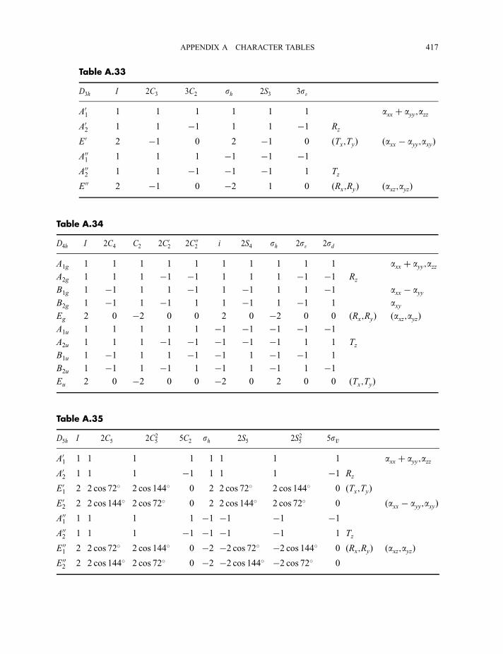
Table A.33
D3h I 2C3 3C2 sh 2S3 3sv
A01 1 1 1 1 1 1 axx þ ayy;azzA02 1 1 �1 1 1 �1 Rz
E0 2 �1 0 2 �1 0 ðTx;TyÞ ðaxx � ayy;axyÞA001 1 1 1 �1 �1 �1A002 1 1 �1 �1 �1 1 Tz
E00 2 �1 0 �2 1 0 ðRx;RyÞ ðaxz;ayzÞ
Table A.34
D4h I 2C4 C2 2C02 2C002 i 2S4 sh 2sv 2sd
A1g 1 1 1 1 1 1 1 1 1 1 axx þ ayy;azzA2g 1 1 1 �1 �1 1 1 1 �1 �1 Rz
B1g 1 �1 1 1 �1 1 �1 1 1 �1 axx � ayyB2g 1 �1 1 �1 1 1 �1 1 �1 1 axyEg 2 0 �2 0 0 2 0 �2 0 0 ðRx;RyÞ ðaxz;ayzÞA1u 1 1 1 1 1 �1 �1 �1 �1 �1A2u 1 1 1 �1 �1 �1 �1 �1 1 1 Tz
B1u 1 �1 1 1 �1 �1 1 �1 �1 1
B2u 1 �1 1 �1 1 �1 1 �1 1 �1Eu 2 0 �2 0 0 �2 0 2 0 0 ðTx;TyÞ
Table A.35
D5h I 2C5 2C25 5C2 sh 2S5 2S25 5sv
A01 1 1 1 1 1 1 1 1 axx þ ayy;azzA02 1 1 1 �1 1 1 1 �1 Rz
E01 2 2 cos 72� 2 cos 144� 0 2 2 cos 72� 2 cos 144� 0 ðTx;TyÞE02 2 2 cos 144� 2 cos 72� 0 2 2 cos 144� 2 cos 72� 0 ðaxx � ayy;axyÞA001 1 1 1 1 �1 �1 �1 �1A002 1 1 1 �1 �1 �1 �1 1 Tz
E001 2 2 cos 72� 2 cos 144� 0 �2 �2 cos 72� �2 cos 144� 0 ðRx;RyÞ ðaxz;ayzÞE002 2 2 cos 144� 2 cos 72� 0 �2 �2 cos 144� �2 cos 72� 0
APPENDIX A CHARACTER TABLES 417
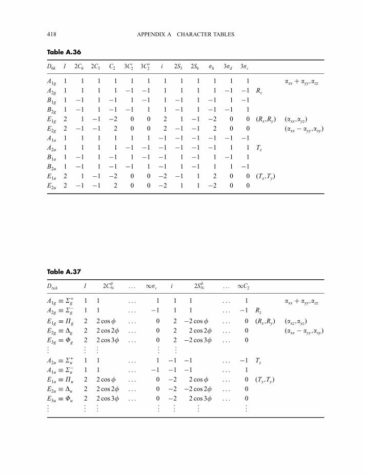
Table A.36
D6h I 2C6 2C3 C2 3C02 3C002 i 2S3 2S6 sh 3sd 3sv
A1g 1 1 1 1 1 1 1 1 1 1 1 1 axx þ ayy;azzA2g 1 1 1 1 �1 �1 1 1 1 1 �1 �1 Rz
B1g 1 �1 1 �1 1 �1 1 �1 1 �1 1 �1B2g 1 �1 1 �1 �1 1 1 �1 1 �1 �1 1
E1g 2 1 �1 �2 0 0 2 1 �1 �2 0 0 ðRx;RyÞ ðaxx;ayzÞE2g 2 �1 �1 2 0 0 2 �1 �1 2 0 0 ðaxx � ayy;axyÞA1u 1 1 1 1 1 1 �1 �1 �1 �1 �1 �1A2u 1 1 1 1 �1 �1 �1 �1 �1 �1 1 1 Tz
B1u 1 �1 1 �1 1 �1 �1 1 �1 1 �1 1
B2u 1 �1 1 �1 �1 1 �1 1 �1 1 1 �1E1u 2 1 �1 �2 0 0 �2 �1 1 2 0 0 ðTx;TyÞE2u 2 �1 �1 2 0 0 �2 1 1 �2 0 0
Table A.37
D1h I 2Cf1 . . . 1sv i 2S
f1 . . . 1C2
A1g Sþg 1 1 . . . 1 1 1 . . . 1 axx þ ayy;azzA2g S�g 1 1 . . . �1 1 1 . . . �1 Rz
E1g Pg 2 2 cosf . . . 0 2 �2 cosf . . . 0 ðRx;RyÞ ðaxz;ayzÞE2g Dg 2 2 cos 2f . . . 0 2 2 cos 2f . . . 0 ðaxx � ayy;axyÞE3g Fg 2 2 cos 3f . . . 0 2 �2 cos 3f . . . 0
..
. ... ..
. ... ..
.
A2u Sþu 1 1 . . . 1 �1 �1 . . . �1 Tz
A1u S�u 1 1 . . . �1 �1 �1 . . . 1
E1u Pu 2 2 cosf . . . 0 �2 2 cosf . . . 0 ðTx;TyÞE2u Du 2 2 cos 2f . . . 0 �2 �2 cos 2f . . . 0
E3u Fu 2 2 cos 3f . . . 0 �2 2 cos 3f . . . 0
..
. ... ..
. ... ..
. ... ..
.
418 APPENDIX A CHARACTER TABLES
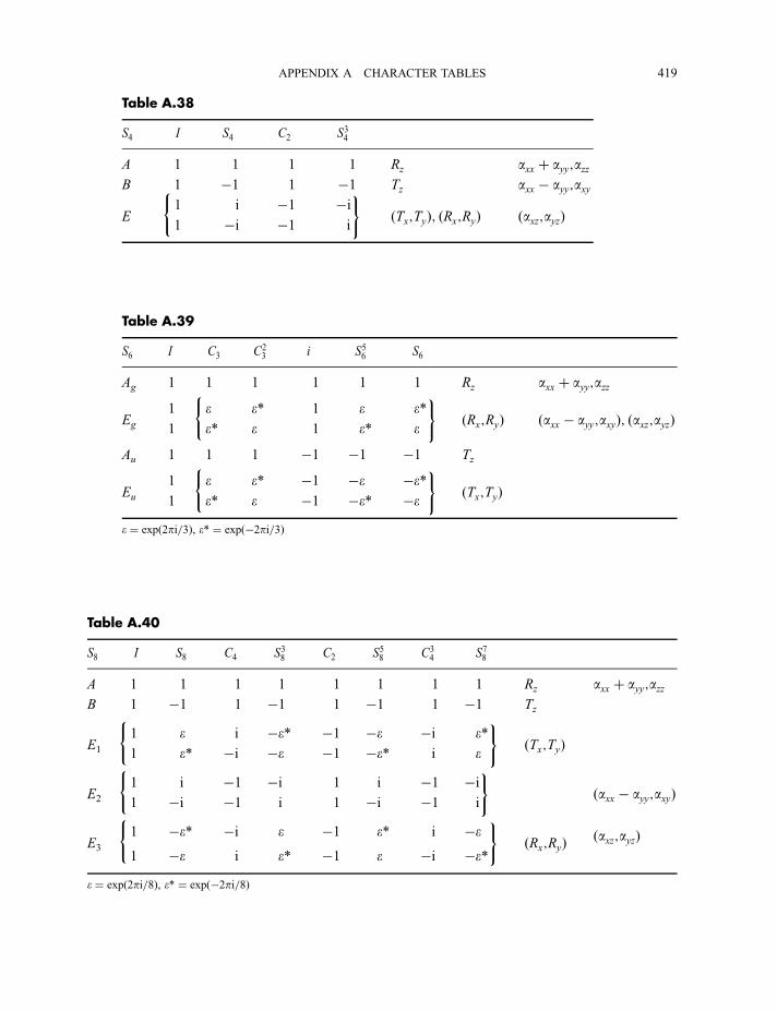
Table A.38
S4 I S4 C2 S34
A 1 1 1 1 Rz axx þ ayy;azzB 1 �1 1 �1 Tz axx � ayy;axy
E
(1 i �1 �i
)ðTx;TyÞ; ðRx;RyÞ ðaxz;ayzÞ1 �i �1 i
Table A.39
S6 I C3 C23 i S56 S6
Ag 1 1 1 1 1 1 Rz axx þ ayy;azz
Eg
1(e e* 1 e e*
)ðRx;RyÞ ðaxx � ayy;axyÞ; ðaxz;ayzÞ1 e* e 1 e* e
Au 1 1 1 �1 �1 �1 Tz
Eu
1(e e* �1 �e �e*
)ðTx;TyÞ1 e* e �1 �e* �e
e ¼ expð2pi=3Þ, e* ¼ expð�2pi=3Þ
Table A.40
S8 I S8 C4 S38 C2 S58 C34 S78
A 1 1 1 1 1 1 1 1 Rz axx þ ayy;azzB 1 �1 1 �1 1 �1 1 �1 Tz
E1
(1 e i �e* �1 �e �i e*
)ðTx;TyÞ1 e* �i �e �1 �e* i e
E2
(1 i �1 �i 1 i �1 �i
)ðaxx � ayy;axyÞ1 �i �1 i 1 �i �1 i
E3
(1 �e* �i e �1 e* i �e
)ðRx;RyÞ ðaxz;ayzÞ
1 �e i e* �1 e �i �e*e ¼ expð2pi=8Þ, e* ¼ expð�2pi=8Þ
APPENDIX A CHARACTER TABLES 419
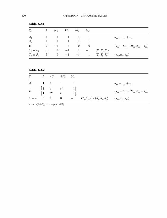
Table A.41
Td I 8C3 3C2 6S4 6sd
A1 1 1 1 1 1 axx þ ayy þ azzA2
1 1 1 �1 �1E 2 �1 2 0 0 ðaxx þ ayy � 2azz;axx � ayyÞT1 F1 3 0 �1 1 �1 ðRx;Ry;RzÞT2 F2 3 0 �1 �1 1 ðTx;Ty;TzÞ ðaxy;axz;ayzÞ
Table A.42
T I 4C3 4C23 3C2
A 1 1 1 1 axx þ ayy þ azz
E
(1 e e* 1
)ðaxx þ ayy � 2azz;axx � ayyÞ1 e* e 1
T F 3 0 0 �1 ðTx;Ty;TzÞ; ðRx;Ry;RzÞ ðaxy;axz;ayzÞe ¼ expð2pi=3Þ, e* ¼ expð�2pi=3Þ
420 APPENDIX A CHARACTER TABLES
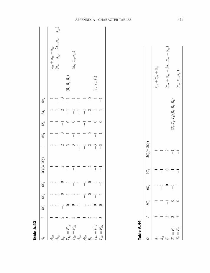
Table
A.4
4
OI
8C3
6C2
6C4
3C0 2ð¼
3C2 4Þ
A1
11
11
1a x
xþa y
yþa z
z
A2
11
�1�1
1
E2
�10
02
ða xxþa y
y�2a z
z;a
xx�a y
yÞ
T1
F1
30
�11
�1ðT
x;T
y;T
zÞðR
x;R
y;R
zÞ
T2
F2
30
1�1
�1ða x
y;a
xz;a
yzÞ
Table
A.4
3
Oh
I8C
36C
26C
43C0 2ð¼
3C2 4Þ
i6S
48S
63s
h6s
d
A1g
11
11
11
11
11
a xxþa y
yþa z
z
A2g
11�1
�11
1�1
11
�1ða x
xþa y
y�2a z
z;a
xx�a y
yÞ
Eg
2�1
00
22
0�1
20
T1g
F1g
30�1
1�1
31
0�1
�1ðR
x;R
y;R
zÞ
T2g
F2g
30
1�1
�13
�10
�11
ða xz;a
yz;a
xyÞ
A1u
11
11
1�1
�1�1
�1�1
A2u
11�1
�11
�11
�1�1
1
Eu
2�1
00
2�2
01
�20
T1u
F1u
30�1
1�1
�3�1
01
1ðT
x;T
y;T
zÞ
T2u
F2u
30
1�1
�1�3
10
1�1
APPENDIX A CHARACTER TABLES 421
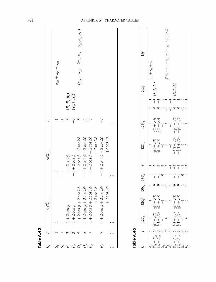
Table
A.4
5
Kh
I1
Cf 1. ..
1Sf 1. ..
i
Sg
11
11
a xxþa y
yþa z
z
Su
11
�1�1
Pg
31þ2cosf
1�2cosf
3ðR
x;R
y;R
zÞ
Pu
31þ2cosf
�1þ2cosf
�3ðT
x;T
y;T
zÞ
Dg
51þ2cosfþ2cos2f
1�2cosfþ2cos2f
5ða x
xþa y
y�2a z
z;a
xx�a y
y;a
xy;a
yzÞ
Du
51þ2cosfþ2cos2f
�1þ2cosf�2cos2f
�5Fg
71þ2cosfþ2cos2f
1�2cosfþ2cos2f
7
þ2cos3f
�2cos3f
Fu
71þ2cosfþ2cos2f
�1þ2cosf�2cos2f
�7þ2cos3f
þ2cos3f
. ... ..
. ... ..
. ..
Table
A.4
6
I hI
12C5
12C
2 520C3
15C2
i12S 1
012
S3 10
20S 6
15s
Ag
11
11
11
11
11
a xxþa y
yþa z
z
T1g
F1g
31 2ð1þp5Þ
1 2ð1�p5Þ
0�1
31 2ð1�p5Þ
1 2ð1þp5Þ
0�1
ðRx;R
y;R
zÞ
T2g
F2g
31 2ð1�p5Þ
1 2ð1þp5Þ
0�1
31 2ð1þp5Þ
1 2ð1�p5Þ
0�1
Gg
4�1
�11
04
�1�1
10
Hg
50
0�1
15
00
�11
ð2azz�a x
x�a y
y;a
xx�a y
y;a
xy;a
yz;a
zxÞ
Au
11
11
1�1
�1�1
�1�1
T1u
F1u
31 2ð1þp5Þ
1 2ð1�p5Þ
0�1
�3�
1 2ð1�p5Þ�
1 2ð1þp5Þ
01ðT
x;T
y;T
zÞ
T2u
F2u
31 2ð1�p5Þ
1 2ð1þp5Þ
0�1
�3�
1 2ð1þp5Þ�
1 2ð1�p5Þ
01
Gu
4�1
�11
0�4
11
�10
Hu
50
0�1
1�5
00
1�1
422 APPENDIX A CHARACTER TABLES
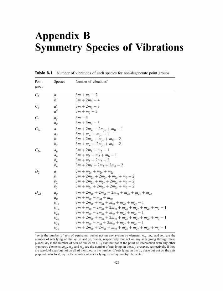
Appendix BSymmetry Species of Vibrations
Table B.1 Number of vibrations of each species for non-degenerate point groups
Point
group
Species Number of vibrationsa
C2 a 3mþ m0 � 2
b 3mþ 2m0 � 4
Cs a0 3mþ 2m0 � 3
a00 3mþ m0 � 3
Ci ag 3m� 3
au 3mþ 3m0 � 3
C2v a1 3mþ 2mxz þ 2myz þ m0 � 1
a2 3mþ mxz þ myz � 1
b1 3mþ 2mxz þ myz þ m0 � 2
b2 3mþ mxz þ 2myz þ m0 � 2
C2h ag 3mþ 2mh þ m2 � 1
au 3mþ mh þ m2 þ m0 � 1
bg 3mþ mh þ 2m2 � 2
bu 3mþ 2mh þ 2m2 þ 2m0 � 2
D2 a 3mþ m2x þ m2y þ m2z
b1 3mþ 2m2x þ 2m2y þ m2z þ m0 � 2
b2 3mþ 2m2x þ m2y þ 2m2z þ m0 � 2
b3 3mþ m2x þ 2m2y þ 2m2z þ m0 � 2
D2h ag 3mþ 2mxy þ 2mxz þ 2myz þ m2x þ m2y þ m2z
au 3mþ mxy þ mxz þ myz
b1g 3mþ 2mxy þ mxz þ myz þ m2x þ m2y � 1
b1u 3mþ mxy þ 2mxz þ 2myz þ m2x þ m2y þ m2z þ m0 � 1
b2g 3mþ mxy þ 2mxz þ myz þ m2x þ m2z � 1
b2u 3mþ 2mxy þ mxz þ 2myz þ m2x þ m2y þ m2z þ m0 � 1
b3g 3mþ mxy þ mxz þ 2myz þ m2y þ m2z � 1
b3u 3mþ 2mxy þ 2mxz þ myz þ m2x þ m2y þ m2z þ m0 � 1
a m is the number of sets of equivalent nuclei not on any symmetry element; mxy, mxz and myz are thenumber of sets lying on the xy, xz and yz, planes, respectively, but not on any axes going through theseplanes; m2 is the number of sets of nuclei on a C2 axis but not at the point of intersection with any othersymmetry elements; m2x, m2y and m2z are the number of sets lying on the x, y or z axes, respectively, if theyare two-fold axes but not on all of them; mh is the number of sets lying on the sh plane but not on the axisperpendicular to it; m0 is the number of nuclei lying on all symmetry elements.
423
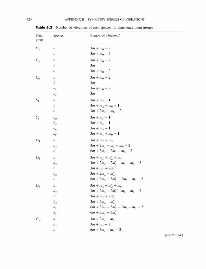
Table B.2 Number of vibrations of each species for degenerate point groups
Point
group
Species Number of vibrationsa
C3 a 3mþ m0 � 2
e 3mþ m0 � 2
C4 a 3mþ m0 � 2
b 3m
e 3mþ m0 � 2
C6 a 3mþ m0 � 2
b 3m
e1 3mþ m0 � 2
e2 3m
S4 a 3mþ m2 � 1
b 3mþ m2 þ m0 � 1
e 3mþ 2m2 þ m0 � 2
S6 ag 3mþ m3 � 1
bu 3mþ m3 � 1
eg 3mþ m3 � 1
eu 3mþ m3 þ m0 � 1
D3 a1 3mþ m2 þ m3
a2 3mþ 2m2 þ m3 þ m0 � 2
e 6mþ 3m2 þ 2m3 þ m0 � 2
D4 a1 3mþ m2 þ m02 þ m4
a2 3mþ 2m2 þ 2m02 þ m4 þ m0 � 2
b1 3mþ m2 þ 2m02b2 3mþ 2m2 þ m02e 6mþ 3m2 þ 3m02 þ 2m4 þ m0 � 2
D6 a1 3mþ m2 þ m02 þ m6
a2 3mþ 2m2 þ 2m02 þ m6 þ m0 � 2
b1 3mþ m2 þ 2m02b2 3mþ 2m2 þ m02e1 6mþ 3m2 þ 3m02 þ 2m6 þ m0 � 2
e2 6mþ 3m2 þ 3m02C3v a1 3mþ 2mv þ m0 � 1
a2 3mþ mv � 1
e 6mþ 3mv þ m0 � 2
(continued )
424 APPENDIX B SYMMETRY SPECIES OF VIBRATIONS
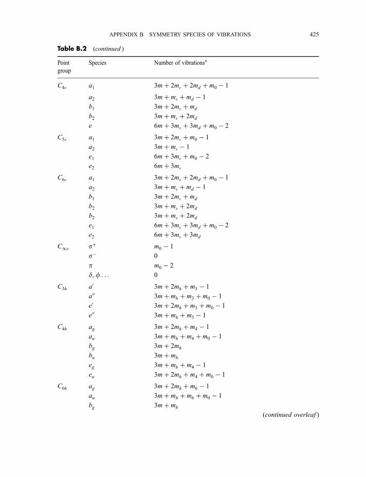
Table B.2 (continued )
Point
group
Species Number of vibrationsa
C4v a1 3mþ 2mv þ 2md þ m0 � 1
a2 3mþ mv þ md � 1
b1 3mþ 2mv þ md
b2 3mþ mv þ 2md
e 6mþ 3mv þ 3md þ m0 � 2
C5v a1 3mþ 2mv þ m0 � 1
a2 3mþ mv � 1
e1 6mþ 3mv þ m0 � 2
e2 6mþ 3mv
C6v a1 3mþ 2mv þ 2md þ m0 � 1
a2 3mþ mv þ md � 1
b1 3mþ 2mv þ md
b2 3mþ mv þ 2md
b2 3mþ mv þ 2md
e1 6mþ 3mv þ 3md þ m0 � 2
e2 6mþ 3mv þ 3md
C1v sþ m0 � 1
s� 0
p m0 � 2
d;f . . . 0
C3h a0 3mþ 2mh þ m3 � 1
a00 3mþ mh þ m3 þ m0 � 1
e0 3mþ 2mh þ m3 þ m0 � 1
e00 3mþ mh þ m3 � 1
C4h ag 3mþ 2mh þ m4 � 1
au 3mþ mh þ m4 þ m0 � 1
bg 3mþ 2mh
bu 3mþ mh
eg 3mþ mh þ m4 � 1
eu 3mþ 2mh þ m4 þ m0 � 1
C6h ag 3mþ 2mh þ m6 � 1
au 3mþ mh þ m6 þ m0 � 1
bg 3mþ mh
(continued overleaf )
APPENDIX B SYMMETRY SPECIES OF VIBRATIONS 425
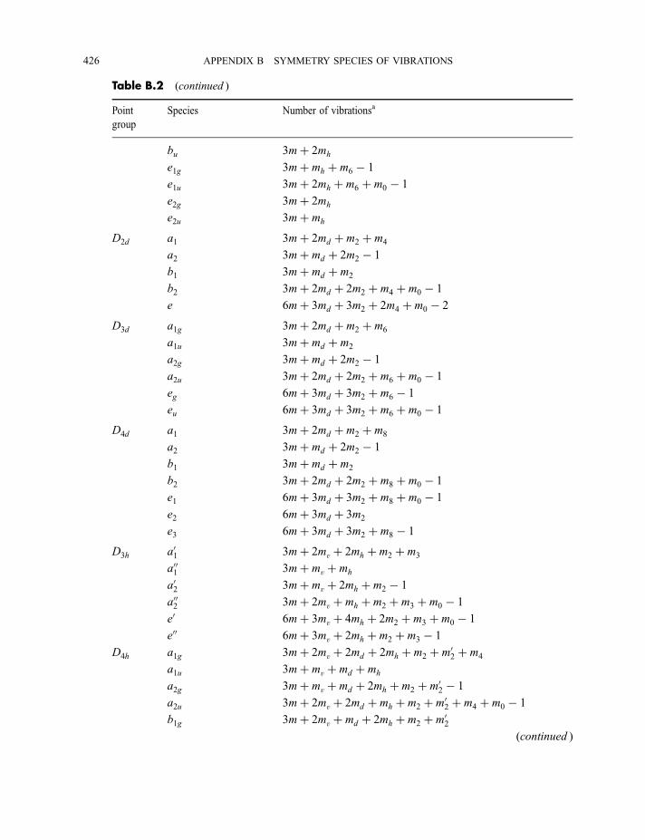
Table B.2 (continued )
Point
group
Species Number of vibrationsa
bu 3mþ 2mh
e1g 3mþ mh þ m6 � 1
e1u 3mþ 2mh þ m6 þ m0 � 1
e2g 3mþ 2mh
e2u 3mþ mh
D2d a1 3mþ 2md þ m2 þ m4
a2 3mþ md þ 2m2 � 1
b1 3mþ md þ m2
b2 3mþ 2md þ 2m2 þ m4 þ m0 � 1
e 6mþ 3md þ 3m2 þ 2m4 þ m0 � 2
D3d a1g 3mþ 2md þ m2 þ m6
a1u 3mþ md þ m2
a2g 3mþ md þ 2m2 � 1
a2u 3mþ 2md þ 2m2 þ m6 þ m0 � 1
eg 6mþ 3md þ 3m2 þ m6 � 1
eu 6mþ 3md þ 3m2 þ m6 þ m0 � 1
D4d a1 3mþ 2md þ m2 þ m8
a2 3mþ md þ 2m2 � 1
b1 3mþ md þ m2
b2 3mþ 2md þ 2m2 þ m8 þ m0 � 1
e1 6mþ 3md þ 3m2 þ m8 þ m0 � 1
e2 6mþ 3md þ 3m2
e3 6mþ 3md þ 3m2 þ m8 � 1
D3h a01 3mþ 2mv þ 2mh þ m2 þ m3
a001 3mþ mv þ mh
a02 3mþ mv þ 2mh þ m2 � 1
a002 3mþ 2mv þ mh þ m2 þ m3 þ m0 � 1
e0 6mþ 3mv þ 4mh þ 2m2 þ m3 þ m0 � 1
e00 6mþ 3mv þ 2mh þ m2 þ m3 � 1
D4h a1g 3mþ 2mv þ 2md þ 2mh þ m2 þ m02 þ m4
a1u 3mþ mv þ md þ mh
a2g 3mþ mv þ md þ 2mh þ m2 þ m02 � 1
a2u 3mþ 2mv þ 2md þ mh þ m2 þ m02 þ m4 þ m0 � 1
b1g 3mþ 2mv þ md þ 2mh þ m2 þ m02(continued )
426 APPENDIX B SYMMETRY SPECIES OF VIBRATIONS
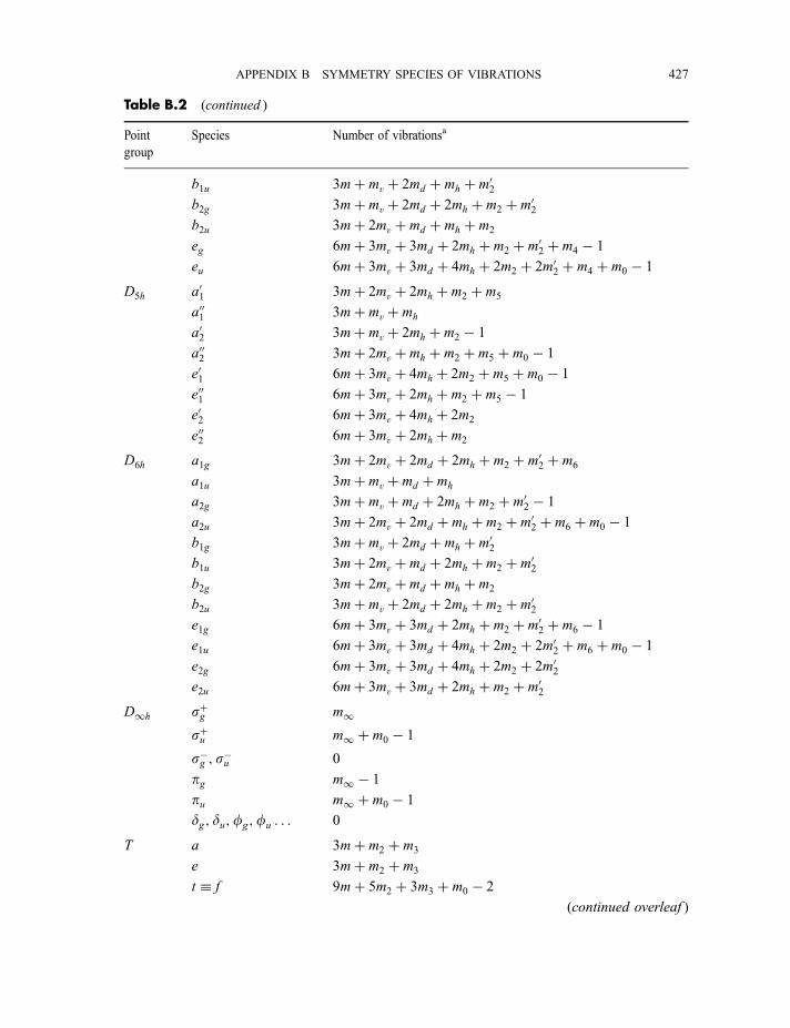
Table B.2 (continued )
Point
group
Species Number of vibrationsa
b1u 3mþ mv þ 2md þ mh þ m02b2g 3mþ mv þ 2md þ 2mh þ m2 þ m02b2u 3mþ 2mv þ md þ mh þ m2
eg 6mþ 3mv þ 3md þ 2mh þ m2 þ m02 þ m4 � 1
eu 6mþ 3mv þ 3md þ 4mh þ 2m2 þ 2m02 þ m4 þ m0 � 1
D5h a01 3mþ 2mv þ 2mh þ m2 þ m5
a001 3mþ mv þ mh
a02 3mþ mv þ 2mh þ m2 � 1
a002 3mþ 2mv þ mh þ m2 þ m5 þ m0 � 1
e01 6mþ 3mv þ 4mh þ 2m2 þ m5 þ m0 � 1
e001 6mþ 3mv þ 2mh þ m2 þ m5 � 1
e02 6mþ 3mv þ 4mh þ 2m2
e002 6mþ 3mv þ 2mh þ m2
D6h a1g 3mþ 2mv þ 2md þ 2mh þ m2 þ m02 þ m6
a1u 3mþ mv þ md þ mh
a2g 3mþ mv þ md þ 2mh þ m2 þ m02 � 1
a2u 3mþ 2mv þ 2md þ mh þ m2 þ m02 þ m6 þ m0 � 1
b1g 3mþ mv þ 2md þ mh þ m02b1u 3mþ 2mv þ md þ 2mh þ m2 þ m02b2g 3mþ 2mv þ md þ mh þ m2
b2u 3mþ mv þ 2md þ 2mh þ m2 þ m02e1g 6mþ 3mv þ 3md þ 2mh þ m2 þ m02 þ m6 � 1
e1u 6mþ 3mv þ 3md þ 4mh þ 2m2 þ 2m02 þ m6 þ m0 � 1
e2g 6mþ 3mv þ 3md þ 4mh þ 2m2 þ 2m02e2u 6mþ 3mv þ 3md þ 2mh þ m2 þ m02
D1h sþg m1sþu m1 þ m0 � 1
s�g ; s�u 0
pg m1 � 1
pu m1 þ m0 � 1
dg; du;fg;fu . . . 0
T a 3mþ m2 þ m3
e 3mþ m2 þ m3
t f 9mþ 5m2 þ 3m3 þ m0 � 2
(continued overleaf )
APPENDIX B SYMMETRY SPECIES OF VIBRATIONS 427
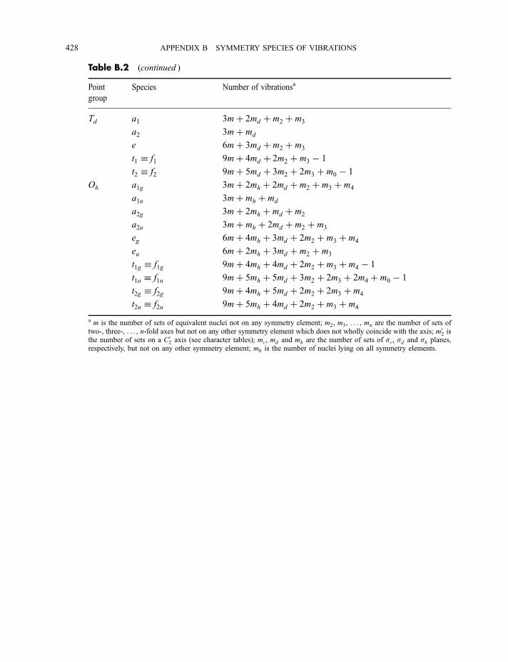
Table B.2 (continued )
Point
group
Species Number of vibrationsa
Td a1 3mþ 2md þ m2 þ m3
a2 3mþ md
e 6mþ 3md þ m2 þ m3
t1 f1 9mþ 4md þ 2m2 þ m3 � 1
t2 f2 9mþ 5md þ 3m2 þ 2m3 þ m0 � 1
Oh a1g 3mþ 2mh þ 2md þ m2 þ m3 þ m4
a1u 3mþ mh þ md
a2g 3mþ 2mh þ md þ m2
a2u 3mþ mh þ 2md þ m2 þ m3
eg 6mþ 4mh þ 3md þ 2m2 þ m3 þ m4
eu 6mþ 2mh þ 3md þ m2 þ m3
t1g f1g 9mþ 4mh þ 4md þ 2m2 þ m3 þ m4 � 1
t1u f1u 9mþ 5mh þ 5md þ 3m2 þ 2m3 þ 2m4 þ m0 � 1
t2g f2g 9mþ 4mh þ 5md þ 2m2 þ 2m3 þ m4
t2u f2u 9mþ 5mh þ 4md þ 2m2 þ m3 þ m4
a m is the number of sets of equivalent nuclei not on any symmetry element; m2, m3, . . . , mn are the number of sets oftwo-, three-, . . . , n-fold axes but not on any other symmetry element which does not wholly coincide with the axis; m02 isthe number of sets on a C02 axis (see character tables); mv, md and mh are the number of sets of sv, sd and sh planes,respectively, but not on any other symmetry element; m0 is the number of nuclei lying on all symmetry elements.
428 APPENDIX B SYMMETRY SPECIES OF VIBRATIONS
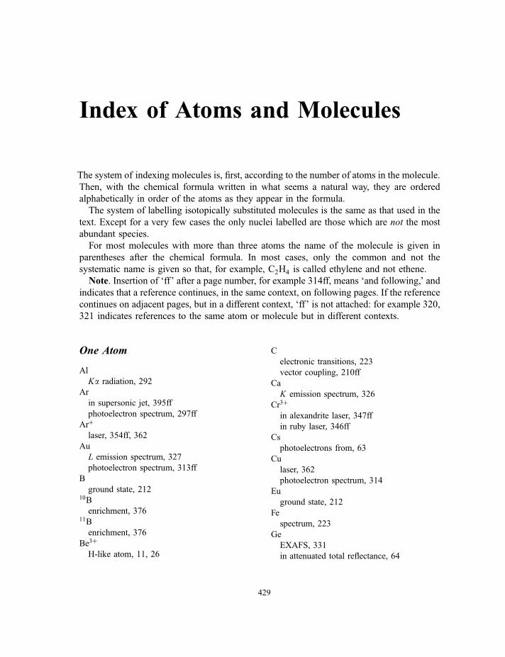
Index of Atoms and Molecules
The system of indexing molecules is, first, according to the number of atoms in the molecule.
Then, with the chemical formula written in what seems a natural way, they are ordered
alphabetically in order of the atoms as they appear in the formula.
The system of labelling isotopically substituted molecules is the same as that used in the
text. Except for a very few cases the only nuclei labelled are those which are not the most
abundant species.
For most molecules with more than three atoms the name of the molecule is given in
parentheses after the chemical formula. In most cases, only the common and not the
systematic name is given so that, for example, C2H4 is called ethylene and not ethene.
Note. Insertion of ‘ff’ after a page number, for example 314ff, means ‘and following,’ and
indicates that a reference continues, in the same context, on following pages. If the reference
continues on adjacent pages, but in a different context, ‘ff’ is not attached: for example 320,
321 indicates references to the same atom or molecule but in different contexts.
One Atom
Al
Ka radiation, 292
Ar
in supersonic jet, 395ff
photoelectron spectrum, 297ff
Arþ
laser, 354ff, 362
Au
L emission spectrum, 327
photoelectron spectrum, 313ff
B
ground state, 21210B
enrichment, 37611B
enrichment, 376
Be3þ
H-like atom, 11, 26
C
electronic transitions, 223
vector coupling, 210ff
Ca
K emission spectrum, 326
Cr3þ
in alexandrite laser, 347ff
in ruby laser, 346ff
Cs
photoelectrons from, 63
Cu
laser, 362
photoelectron spectrum, 314
Eu
ground state, 212
Fe
spectrum, 223
Ge
EXAFS, 331
in attenuated total reflectance, 64
429
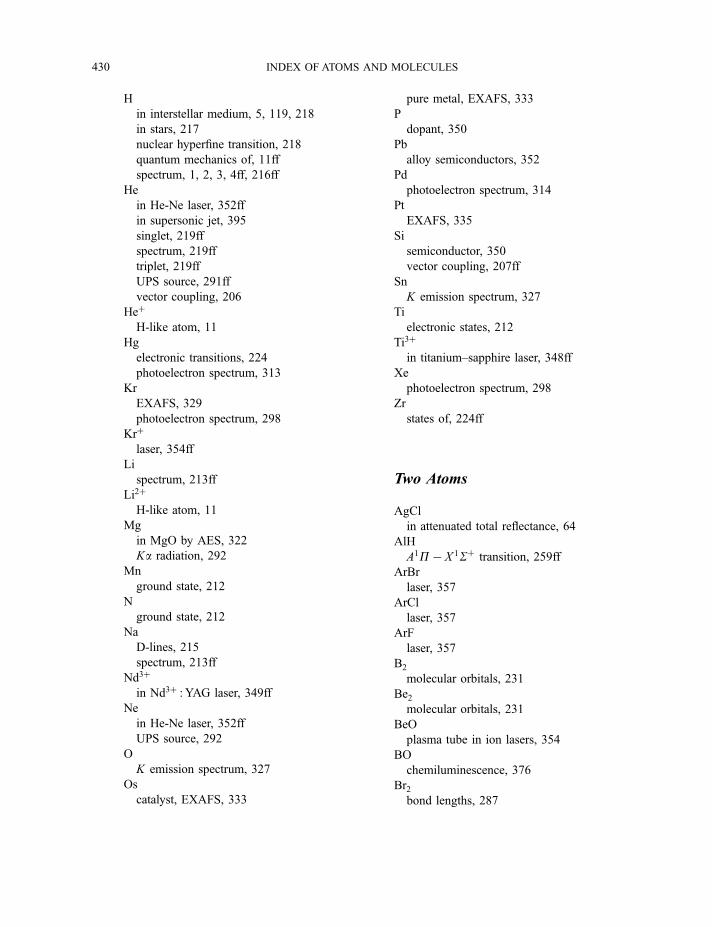
H
in interstellar medium, 5, 119, 218
in stars, 217
nuclear hyperfine transition, 218
quantum mechanics of, 11ff
spectrum, 1, 2, 3, 4ff, 216ff
He
in He-Ne laser, 352ff
in supersonic jet, 395
singlet, 219ff
spectrum, 219ff
triplet, 219ff
UPS source, 291ff
vector coupling, 206
Heþ
H-like atom, 11
Hg
electronic transitions, 224
photoelectron spectrum, 313
Kr
EXAFS, 329
photoelectron spectrum, 298
Krþ
laser, 354ff
Li
spectrum, 213ff
Li2þ
H-like atom, 11
Mg
in MgO by AES, 322
Ka radiation, 292
Mn
ground state, 212
N
ground state, 212
Na
D-lines, 215
spectrum, 213ff
Nd3þ
in Nd3þ : YAG laser, 349ff
Ne
in He-Ne laser, 352ff
UPS source, 292
O
K emission spectrum, 327
Os
catalyst, EXAFS, 333
pure metal, EXAFS, 333
P
dopant, 350
Pb
alloy semiconductors, 352
Pd
photoelectron spectrum, 314
Pt
EXAFS, 335
Si
semiconductor, 350
vector coupling, 207ff
Sn
K emission spectrum, 327
Ti
electronic states, 212
Ti3þ
in titanium–sapphire laser, 348ff
Xe
photoelectron spectrum, 298
Zr
states of, 224ff
Two Atoms
AgCl
in attenuated total reflectance, 64
AlH
A1P� X 1Sþ transition, 259ff
ArBr
laser, 357
ArCl
laser, 357
ArF
laser, 357
B2
molecular orbitals, 231
Be2molecular orbitals, 231
BeO
plasma tube in ion lasers, 354
BO
chemiluminescence, 376
Br2bond lengths, 287
430 INDEX OF ATOMS AND MOLECULES
EXAFS, 329
on graphite, SEXAFS, 333
BrO
in atmosphere, 385
C2
D1Sþu � X 1Sþg system, 246
by multiphoton dissociation, 374
dissociation, 240ff
electronic transitions, 242
molecular orbitals, 231ff
potential energy curves, 240ff
Swan bands, 240
CdH
bond lengths, 287
CH
bond lengths, 287
interstellar, 120
CHþ
interstellar, 120
Cl2force constant, 138ff
ClO
in atmosphere, 385
CN
interstellar, 120
molecular orbitals, 232
CO
a3P� X 1Sþ transition, 236
A1P� X 1Sþ transition, 250ff
adsorbed on Cu, 64
dipole moment, 116
force constant, 138
interstellar, 120
laser, 362, 368
molecular orbitals, 232
photoelectron spectrum, 307ff
rotational energy levels, 22, 106ff
rotational spectrum, 106ff
vibration-rotation Raman spectrum, 152
vibrational energy levels, 144ff
COþ
interstellar, 120
CP
interstellar, 120
CS
interstellar, 120
CuH
A1Sþ � X 1Sþ transition, 256ff
F2force constant, 138
molecular orbitals, 231ff
nuclear spin, 129ff, 153
H2
dissociation, 254
molecular orbitals, 231
nuclear spin, 129ff, 153
ortho and para forms, 129ffphotoelectron spectrum, 298ff
repulsive state, 2541H2H
dipole moment, 1062H2
nuclear spin, 130ff, 153
Hþ2one-electron molecule, 11
HBr
photoelectron spectrum, 302ff
HBrþ
bond lengths, 303
HCl
anharmonic constants, 144
force constant, 138
interstellar, 120
molecular orbitals, 233
photoelectron spectrum, 302ff
rotational, vibrational constants, 151
vibration–rotation spectrum, 148ff, 152ff
vibration wavenumber, 26, 1441H37Cl
vibration–rotation spectrum, 148ff2H35Cl
vibration–rotation spectrum, 195
He2bound excited states, 254, 356
molecular orbitals, 231
repulsive ground state, 253, 356
HF
dipole moment, 106
force constant, 138
HI
photoelectron spectrum, 303
INDEX OF ATOMS AND MOLECULES 431
I2B3P0þu � X 1Sþg transition, 237, 245, 248,
252ff
wave packet spectroscopy, 392ff
IO
A2P3=2 � X 2P3=2 system, 386
in atmosphere, 385ff
KBr
disk, 62, 158
windows for infrared, 62
KrBr
laser, 357
KrCl
laser, 357
KrF
laser, 357
KrI
laser, 357
Li2molecular orbitals, 231
LiF
diffraction of X-rays, 323
transparency in ultraviolet, 63
MgO
Auger electron spectrum, 322
N2
bond length, 132, 246, 301, 355
in excited states, 246, 355
C3Pu � B2Pg system, 245
force constant, 138
in CO2 laser, 358ff
Koopmans’ theorem, 297, 302
laser, 355ff
molecular orbitals, 231
nuclear spin, 129ff, 153
photoelectron spectrum, 300ff14N15N
rotational Raman spectrum, 133ff15N2
bond length, 132
rotational Raman spectrum, 128
Nþ2bond lengths, 301
NaCl
Auger electron spectrum, 320ff
windows for infrared, 62
NaI
transition state, 389ff
Ne2molecular orbitals, 231
NeF
laser, 357
NH
interstellar, 120
NO
force constant, 138
interstellar, 120
molecular orbitals, 232
photoelectron spectrum (on Fe), 303ff, 314ff
NOþ
electronic states, 303ff
NS
interstellar, 120
O2
a1Dg � X 3S�g system, 384ff
b1Sþg � X 3S�g system, 384ff
electronic states, 239
far-ultraviolet absorption, 63
force constant, 138
molecular orbitals, 231ff
nuclear spin, 131, 153
OH
interstellar, 120
PN
vibration wavenumber, 26
PO
molecular orbitals, 232ff
SiC
interstellar, 120
SiF
by multiphoton dissociation, 374
SiO
interstellar, 120
mirror coating, 339
SiS
interstellar, 120
SO
interstellar, 120
molecular orbitals, 232ff
vibration wavenumber, 26
SOþ
interstellar, 120
432 INDEX OF ATOMS AND MOLECULES
TlBr=TlIin attenuated total reflectance, 64
Xe2laser, 357
XeBr
laser, 357
XeCl
laser, 357, 381ff
XeF
laser, 357, 362
XeI
laser, 357
Three Atoms
Ar���HClin supersonic jet, 396
BeH2
molecular orbitals, 261ff
BH2
molecular orbitals, 261ff
CH2
molecular orbitals, 261ff~XX 3B1=~aa1A1 separation, 265
C2H
interstellar, 120
CO2
atmospheric, 379
bending vibration, 93
laser, 358ff, 374ff
local mode behaviour, 188
photoelectron spectrum, 307ff
potential energy surface, 184ff
vibrational constants, 196
CS2solvent for infrared spectra, 62
FNO
laser Stark spectrum, 369
H3
shape, 265
Hþ3shape, 265
H2Dþ
interstellar, 120
HCN
bending vibration, 93
CRDS spectrum, 387
Doppler broadening, 39
interstellar, 120
laser, 362
principal axes, 103ff
symmetry elements, 74, 83
vibration–rotation bands, 175
HCO
interstellar, 120
HCOþ
interstellar, 120
HCSþ
interstellar, 120
HNC
interstellar, 120
HNO
interstellar, 120
H2O
cartesian axes, 89
dipole moment, 97ff, 99, 168
interstellar, 120
laser, 362
molecular orbitals, 264
photoelectron spectrum, 305ff
rotations, 88
symmetry elements, 74, 83
translations, 88
vibrations, 89ff, 167, 170ff
H2Oþ
bond angle, 305
molecular orbitals, 264
H2S
interstellar, 120
LiH2
molecular orbitals, 264
NH2
by multiphoton dissociation, 374
from photolysis of NH3, 67
molecular orbitals, 264
N2Hþ
interstellar, 120
O3
atmospheric, 384
Hartley system, 380
Huggins system, 380
INDEX OF ATOMS AND MOLECULES 433
OCS
Auger electron spectrum, 320
dipole moment, 116
interstellar, 120
SO2
Auger electron spectrum, 320
interstellar, 120
TiO2
mirror coating, 339
Four Atoms
Ar���CO2
in supersonic jet, 396
BCl3 (boron trichloride)
multiphoton dissociation, 376
BF3 (boron trifluoride)
dipole moment, 99, 100
symmetry elements, 75, 76ff, 84
C2H2 (acetylene)
excited electronic state, 261
nuclear spin, 131, 176ff
symmetry elements, 84ff
vibration–rotation bands, 176ff
vibrations, 167, 172, 173
C21H2H (acetylene)
dipole moment, 108
C3H (cyclic)
interstellar, 120
C3H (linear)
interstellar, 120
C3N
interstellar, 120
H2CO (formaldehyde)~AA1A2 � ~XX 1A1 transition, 278, 282
interstellar, 120
molecular orbitals, 265ff
principal axes, 103
structure determination, 132ff
vibrations, 90ff
H2CS (thioformaldehyde)
interstellar, 120
HNCO (fulminic acid)
interstellar, 120
HNCS (thiofulminic acid)
interstellar, 120
H2O2 (hydrogen peroxide)
chirality, 80
symmetry elements, 82
NF3 (nitrogen trifluoride)
dipole moment, 98, 99
NH3 (ammonia)
dipole moment, 97, 98
flash photolysis of, 67
interstellar, 120
inversion, 189ff
barrier height, 190
multiphoton dissociation, 374
symmetry elements, 83
vibrations, 92ff, 171, 173
Five Atoms
Al2O3 (aluminium oxide)
in ruby laser, 346
in titanium–sapphire laser, 348
C3H2 (cyclic)
interstellar, 120
C3H2 (linear)
interstellar, 120
CCl2F2 (dichlorodifluoromethane)
multiphoton dissociation, 374
CH4 (methane)
photoelectron spectrum, 312ff
principal axes, 105
symmetry elements, 85
CHþ4symmetric stretch, 312ff
C4H
interstellar, 120
CHBrClF (bromochlorofluoromethane)
dipole moment, 99ff
enantiomers, 79
symmetry elements, 79ff
CH2F2 (difluoromethane)
cartesian axes, 89
symmetry elements, 77, 83
CH3F (methyl fluoride)
dipole moment, 116
symmetry elements, 74, 83
C2H3F (methyl fluoride)
vibration–rotation band, 178
434 INDEX OF ATOMS AND MOLECULES
CH3I (methyl iodide)
principal axes, 103ff
rotation, 113
CH2NH (methanimine)
interstellar, 120
Cr2O3 (chromium trioxide)
in alexandrite laser, 347ff
in ruby laser, 346ff
HC3N (cyanoacetylene)
interstellar, 120
HCOOH (formic acid)
interstellar, 120
NH2CN (cyanamide)
interstellar, 120
[PtCl4]2�
symmetry elements, 76, 84
SiF4 (silicon tetrafluoride)
multiphoton dissociation, 374
SiH4 (silane)
dipole moment, 118
rotational spectrum, 118
symmetry elements, 85
SiH3F (silyl fluoride)
vibration-rotation band, 179
Six Atoms
C5H
interstellar, 120
C2Cl4 (tetrachloroethylene)
solvent for infrared spectra, 62
C2H4 (ethylene)
symmetry elements, 73, 84
torsion, 173, 195
vibration-rotation bands, 181
CH3CN (methyl cyanide)
interstellar, 120
CH3NC (methyl isocyanide)
interstellar, 120
C2H3F (fluoroethylene)
dipole moment, 98
symmetry elements, 73, 83
C2H2F2 (1,1-difluoroethylene)
symmetry elements, 73, 83
C2H2F2 (cis-1,2-difluoroethylene)dipole moment, 98
symmetry elements, 73, 83
C2H2F2 (trans-1,2-difluoroethylene)dipole moment, 99
symmetry elements, 73, 84
(CHO)2 (s-trans-gyoxal)symmetry elements, 84
CH3OH (methyl alcohol)
interstellar, 120
torsion, 195
CH3SH (methanthiol)
interstellar, 120
HC2CHO
interstellar, 120
HC3NHþ
interstellar, 120
(H2O)2in supersonic jet, 396
N2H4 (hydrazine)
multiphoton dissociation, 375
NH2CHO (formamide)
interstellar, 120
inversion barrier, 191
XeOF4symmetry elements, 74, 83
Seven Atoms
BeAl2O4 (chrysoberyl)
in alexandrite laser, 347
C6H
interstellar, 120
CH2¼C¼CH2 (allene)
symmetric rotor, 105
symmetry elements, 75, 76, 84
CH3C2H (methyl acetylene)
interstellar, 120
CH2CHCN (cyanoethylene)
interstellar, 120
CH3CHO (acetaldehyde)
interstellar, 120
CH3NH2 (methylamine)
interstellar, 120
multiphoton dissociation, 375
CH3NO2 (nitromethane)
torsion, 195
INDEX OF ATOMS AND MOLECULES 435
HC5N (cyanodiacetylene)
interstellar, 120
rotational spectrum, 110
Na2S2O3 (sodium thiosulphate)
Auger electron spectrum, 319
SF6 (sulphur hexafluoride)Auger electron spectrum, 320
multiphoton dissociation, 376
principal axes, 105
symmetry elements, 76, 8534SF6
enrichment, 376
SiH3NCS (silyl isothiocyanate)
rotational spectrum, 115
Eight Atoms
C2H6 (ethane)
hyper-Raman spectrum, 364ff
symmetry elements, 84
torsion, 195, 365
CH2¼CHCCH (vinyl acetylene)
vibrations, 157
CH2¼CHCHO (s-trans-acrolein)principal axes, 105
C2H2Cl2F2 (1,2-dichloro-1,2-difluoroethane)
symmetry elements, 83
CH3C3CN (methyl cyanoacetylene)
interstellar, 120
C2H2N4 (s-tetrazine)~AA1B3u � ~XX 1Ag transition, 397ff
HCOOCH3 (methyl formate)
interstellar, 120
KH2PO4 (potassium dihydrogen phosphate,
KDP)
harmonic generation, 346, 364
Q-switching, 343
K2H2PO4 (potassium dideuterium phosphate,
KD*P)
harmonic generation, 346, 364
Q-switching, 343
Li3NbO4 (lithium niobate)
harmonic generation, 346
Nine Atoms
CH3C4H (methyl diacetylene)
interstellar, 120
C4H4O (furan)
photoelectron spectrum, 310ff
CH3OCH3 (dimethyl ether)
interstellar, 120
C2H5OH (ethyl alcohol)
interstellar, 120
vibrations, 156
CH3CH2CN (cyanoethane)
interstellar, 120
C4H4S (thiophene)
photoelectron spectrum, 310ff
HC7N (cyanotriacetylene)
interstellar, 120
Ni(CO)4 (nickel tetracarbonyl)
molecular orbitals, 270ff
symmetry elements, 85
Ten Atoms
CH2¼CHCH¼CH2 (s-cis-buta-1,3-diene)torsion, 195
CH2¼CHCH¼CH2 (s-trans-buta-1,3-diene)symmetry elements, 76, 84
torsion, 195
C4H4N2 (pyrazine)
laser fluorescence, 377ff
principal axes, 105
C42H4N2 (perdeuteropyrazine)
laser fluorescence, 377ff
C4H5N (pyrrole)
photoelectron spectrum, 310ff
CH3COCH3 (acetone)
photoelectron spectrum, 308ff
Eleven Atoms
CH3CH¼CHCHO (s-trans-crotonaldehyde)infrared spectrum, 159ff
Raman spectrum, 159ff
HC9N (cyanotetraacetylene)
interstellar, 120
436 INDEX OF ATOMS AND MOLECULES
Twelve Atoms
C4H8 (cyclobutane)
ring-puckering, 191
C6H6 (benzene)~AA1B2u � ~XX 1A1g transition, 279, 282
chromophore, 278
local mode behaviour, 187ff
molecular orbitals, 267ff
photoelectron spectrum, 305ff
pressure broadening, 38
principal axes, 105
stimulated Raman spectrum, 365ff
symmetry elements, 74, 84
vibrations, 166
C2H5CH¼CH2 (but-1-ene)
molecular orbitals, 367
CH3CH¼CHCOOH (s-cis-crotonic acid)
rotational spectrum, 117
CH3CH¼CHCOOH (s-trans-crotonic acid)
rotational spectrum, 117
C6H5Cl (chlorobenzene)~AA1B2 � ~XX 1A1 transition, 279ff
C6H5F (fluorobenzene)
vibration–rotation bands, 183
C6H4ClF (2-chlorofluorobenzene)
dipole moment, 98
vibrations, 156
C6H4F2 (1,4-difluorobenzene)~AA1B2u � ~XX 1Ag transition, 283, 372ff
ZEKE-PE spectrum, 403ff
C6H3F3 (1,2,3-trifluorobenzene)
symmetry elements, 100ff
C6H3F3 (1,2,4-trifluorobenzene)
symmetry elements, 100ff
C6H3F3 (1,3,5-trifluorobenzene)
symmetry elements, 100ff
C6H2F4 (1,2,4,5-tetrafluorobenzene)~AA1B2u � ~XX 1Ag transition, 400
symmetry elements, 100ff
C6H2Br2F2 (1,4-dibromo-2,5-difluorobenzene)
symmetry elements, 100ff
C6F6 (hexafluorobenzene)
symmetry elements, 100ff
(NH4)H2PO4 (ammonium dihydrogen
phosphate, ADP)
harmonic generation, 346, 364
Q-switching, 343
More than Twelve Atoms
C5H8 (cyclopentene)
ring-puckering, 191ff
C5H4F4 (tetrafluorospiropentane)
achiral, 80
C6H6OH (phenol)
torsion, 195
vibrations, 158
[Fe(CN)6]3� (ferricyanide ion)
symmetry elements, 85
[Fe(CN)6]4� (ferrocyanide ion)
molecular orbitals, 270ff
HC11N (cyanopentaacetylene)
interstellar, 120
B5H9 (pentaborane-9)
photoelectron spectrum, 311ff
CF3COOC2H5 (ethyl trifluoracetate)
photoelectron spectrum, 310
CH3CHFCHFCH3 (2,3-difluorobutane)
chirality, 80ff
C6H5NH2 (aniline)
fluorescence excitation spectrum, 398ff
inversion barrier, 191
structure, 133
symmetry elements, 83
C6H5CHO (benzaldehyde)
CHO chromophore, 278
KB5O8 (potassium pentaborate, KPB)
harmonic generation, 346
Ar���C6H5NH2 (aniline argon)
fluorescence excitation spectrum, 398ff
structure, 398ff
C6H5CH3 (toluene)
dipole moment, 98
torsion, 195
C6H3(OH)3 (1,3,5-trihydroxybenzene)
symmetry elements, 84
C6H5CH¼CH2 (styrene)
torsion, 195, 401ff
INDEX OF ATOMS AND MOLECULES 437
(C2H2N4)2 (s-tetrazine dimer)
electronic spectrum, 397ff
C10H8 (naphthalene)
symmetry elements, 75, 84
[Cr(H2O)6]2þ
molecular orbitals, 273
[Cr(H2O)6]3þ
molecular orbitals, 272
B12H�12
Ih point group, 86
C6H12O6 (glucose)
chiral, 79
C14H10 (anthracene)
~AA1B1u � ~XX 1Ag transition, 285
C14H10 (phenanthrene)
symmetry elements, 83
C10H14O (carvone)
chiral, 79
[Co(H2NCH2CH2NH2)3]3þ
chiral, 80
symmetry elements, 83
(C6H4NHS)3Mo (tris(2-
aminobenzenethiolate)MoVI)
EXAFS, 331
C20H20
Ih point group, 86ff
CFCs (chlorofluorocarbons)
in atmosphere, 379
C60
Ih point group, 86ff
Rhodamine B
in dye laser, 359ff
Rubredoxins
EXAFS, 331ff
Ferredoxins
bacterial, EXAFS, 331ff
plant, EXAFS, 331ff
438 INDEX OF ATOMS AND MOLECULES
Subject Index
Note. Insertion of ‘ff’ after a page number, for example 341ff, means ‘and following,’ and
indicates that a subject continues, in the same context, on following pages. If the subject
appears on adjacent pages, but in a different context, ‘ff’ is not attached: for example 320,
321 indicates the same subject but in different contexts.
A-type band, of asymmetric rotor, 181,
284, 378AES (Auger electron spectroscopy), 315ff
selection rules, 325
ATR (attenuated total reflectance), 64
AlKa radiation, 292
Absorbance, 33, 68
Absorption, of radiation, 27ff
Absorption coefficient, 33
in EXAFS, 328, 330
Absorption spectroscopy, 42ff
Absorptivity, 33
Acoustic modulator, 344
Actinides, 201
Action, 9
Active medium, 337ff
Adiabatic ionization energy, 299ff
Aerosol
atmospheric, 380
in plasma torch, 66
Alexandrite laser, 347, 348
Alkali metals, 201
photoelectrons from, 289
spectra, 213ff
Alkaline earth metals, 201
spectra, 219ff
Allowed transition, 33
Alloy, photoelectron spectrum of, 314ff
Amplitude, 27, 49
Amplification, in laser, 337
Angle-bending wavenumbers, 157
Angular momentum, 4
change on ionization, 296
coupling in atoms, 205ff
electron spin, 17ff, 204ff, 207ff, 234ff
nuclear spin, 17ff
orbital, 11ff, 17, 204ff, 206ff, 234ff, 257ff
rotational, 21, 257ff
total, 21, 176, 204ff, 208ff, 257
vibrational, 176
Angular wave functions, of H atom, 12ff, 16ff
Anharmonicity
diatomics, 142ff, 241ff, 249
electrical, 142
in multiphoton dissociation, 374
mechanical, 142ff
polyatomics, 186ff
Antibonding orbital, 229
Anti-Stokes Raman scattering, 122, 125ff,
140ff
Antisymmetric, to symmetry operation, 87
Antisymmetric part, of direct product, 95
Arc, 66
Argon ion laser, 354ff, 362
Associated Laguerre functions, 13
Associated Legendre functions, 13
Asymmetric rotor, 105
Atomic absorption, 64ff
Atomic beam, 37
Atomic spectroscopy, 199ff
Attenuated total reflectance, 64
Attenuator, 68
439
Aufbau priciple, 201, 226, 264
Auger electron, 316, 333
Auger electron spectroscopy, 3, 315ff
Avoided crossing, 389ff
Axial modes, of laser cavity, 341ff, 344
Axis of symmetry
Cn, 74
Sn, 76ff
Azimuth, 12
Azimuthal quantum number, 12ff
B-type band, of asymmetric rotor, 181, 283
Background radiation, in universe, 119, 218
Back-scattering amplitude, 330
Backward wave oscillator, 59
Balmer, J.J., 1
Balmer series, 1, 5
Band, definition, 139, 242
Band centre, 148
Band gap, 350ff
Band system, definition, 242
Barrier
inversion, 189ff
puckering, 192
torsion, 192ff
Beam
effusive, 37, 393
supersonic, 393ff
Beamsplitter, 55, 62
Beat frequency, 50
Beer–Lambert law, 33, 328, 383
Bending vibrations, 154ff
Big bang, 119
Birefringence, 343
Birge–Sponer extrapolation, 145, 250
Black body radiation, 4, 6
Blaze angle, 47
Blazed diffraction grating, 46ff
Blue shift, 266
Bohr, N.H.D., 4
Bohr orbit, radius of, 13, 26
Bohr theory, of H atom, 4ff, 17
Bolometer detector, 62, 63
Boltzmann distribution law, 30
Boltzmann population, 30ff, 34, 110ff, 112,
139, 151, 243ff, 257, 337, 360, 396
Bond order, 231
Bond moment, 97
Bond-stretching wavenumbers, 157
Born, M., 9, 20
Born–Oppenheimer approximation, 20ff, 247ff
Bose–Einstein statistics, 129
Boson, 129, 220
Branch, rotational, 127
Bremsstrahlung, 292, 327
Brewster’s angle, 354
Brightness, of laser beam, 339
Building-up principle, 201, 226, 264
Bunching, of electrons in synchrotron, 293
Bunsen, R.W., 1
Butterfly vibration, 400
Ci character table, 408
Cn axis of symmetry, 74
Cn point groups, 82
Cnh point groups, 84
Cnv point groups, 83
Cs character table, 407
C1 character table, 408
C2 character table, 408
C3 character table, 408
C4 character table, 408
C5 character table, 409
C6 character table, 409
C7 character table, 409
C8 character table, 410
C2h character table, 413
C3h character table, 413
C4h character table, 413
C5h character table, 414
C6h character table, 414
C2v character table, 410
C3v character table, 410
C4v character table, 410
C5v character table, 411
C6v character table, 411
C1v character table, 411
C-type band, of asymmetric rotor, 181, 284,
378
CARS (coherent anti-stokes Raman
spectroscopy), 367ff
CCD (charge-coupled device), 63
440 SUBJECT INDEX
CRDS (cavity ring-down spectroscopy), 382ff
CSRS (coherent Stokes Raman spectroscopy),
368
CW (continuous wave) laser, 341
Cassagrain telescope, 379ff
Carbon dioxide laser, 358ff, 374ff
Cavity, of laser, 337ff
Cavity modes, of laser, 341ff
Centre burst, 57
Centre of inversion, 76
Centrifugal distortion
diatomics, 111ff, 127, 151
linear polyatomics, 111ff, 127
symmetric rotors, 114ff
Character, with respect to symmetry operation,
87ff
Character tables, 87ff, 407ff
Charge-coupled device, 63
Chemical lasers, 362
Chemical shift
in AES, 319
in XPS, 307
Chirality, 78ff
symmetry rule, 79ff
Chromophore, 278
Circular polarization, by Pockels cell, 343
Class, of symmetry element, 92
Closed shell molecule, 277
Cluster, 397
Coherence of laser beam, 339
spatial, 339
temporal, 339
Coherent anti-Stokes Raman scattering, 367ff
Coherent Stokes Raman scattering, 368
Co-latitude, 12
Collimation, of supersonic beam, 396
Collision diameter, 38
Collision rate, 38
Colour, of complex ions, 272
Colour centre laser, 362
Combination differences, 150ff, 174, 250, 260
Combination tone, 155
Complex conjugate, 9, 227
Compound doublet, 216
Compound triplet, 222
Condon, E.V., 247
Conduction band, of semiconductor, 62, 350ff
Conductor, of electricity, 350
Configuration, electronic, 201, 210
Congestion, of bands, 285
Continuous spectrum, 253ff
Continuum, in electronic spectrum, 248
Conventions
cartesian axes, 89
inertial axes labels, 103
molecular electronic state labels, 236, 264,
355
prime (0) and double prime (00), 5rotational branch labels, 127ff
symmetry species labels, 88, 92ff, 96
upper=lower states, 5, 144, 236, 246vibrational numbering, 93
vibrational transition labels, 167
vibronic transition labels, 279
Coolidge tube, 322
Core orbitals, 290
Core term, 311
Coriolis forces, 176, 179, 180
Correlation, of electrons, 296
Costain, C.C., 37
Coulomb integral, 228, 267
Coulombic
attractions, 199
repulsions, 199
Coupling, of momenta
atoms, 201ff
diatomic molecules, 233ff
Crystal diode rectifier, 60
Crystal field orbitals, 271ff, 346ff, 348, 349ff
Crystal monochromator, 292, 329
Cutting, of metal, 339
Cylindrical analyser (127�), 294Czerny–Turner grating mount, 61, 63
DF (dispersed fluorescence), 377ff
DIAL (differential absorption LIDAR), 380ff
D lines, of Na, 215ff
d Orbitals of H atom, 16ff
Dn point groups, 83
Dnd point groups, 84
Dnh point groups, 84ff
D2 character table, 411
D3 character table, 412
D4 character table, 412
D5 character table, 412
D6 character table, 412
SUBJECT INDEX 441
D2d character table, 415
D3d character table, 415
D4d character table, 415
D5d character table, 416
D6d character table, 416
D2h character table, 416
D3h character table, 417
D4h character table, 417
D5h character table, 417
D6h character table, 418
D1h character table, 418
Damping, of EXAFS signal, 333
Davisson, C.J., 6
de Broglie, L., 6
Debye unit, 98
Debye–Waller function, 330
Degeneracy
angular wave functions of H atom, 15
in Boltzmann distribution, 30
rotational levels of a diatomic, 21, 110ff
Degrading, of band, 256
Deslandres table, 250
Depolarization ratio, 159ff
Detector, 42ff
bolometer, 62, 63
crystal diode, 60
gas flow, 323
Golay cell, 61, 62
photodiode, 63
photographic plate, 63
photomultiplier, 63
pyroelectric, 62
semiconductor, 62, 323
scintillation counter, 323
thermocouple, 62
Deuterium discharge lamp, 62
Dextro form, 78
Dielectric, mirror coating, 339
Diffraction
electron, 6ff, 329
light, 8
slit, 44ff
Diffraction grating, 45ff, 61, 62, 63
blaze angle, 47
Diffuse series, in alkali metal spectrum, 213ff
Diffuse spectra, 284ff
Dihedral axes, 76
Diode laser, 350ff
Dipole moment
condition for non-zero value, 99ff
induced, 125ff, 345
operator, 31
Stark effect, 59ff, 115ff, 117
symmetry rule, 99
variation with vibration, 139
Dipole selection rules, 166ff
Dirac, P.A.M., 9, 18, 217
Directionality, of laser beam, 339
Direct product, 91
Disorder, in crystal, 330
Dispersed fluorescence, 377ff
Dispersing element, 43ff
Dispersion
angular, 44, 46
linear, 44
Dissociation energy, 143ff, 240
determination, 250ff
Dissociative vibrations, 186
Dopant, in semiconductor, 350ff
Doping, of semiconductor, 350ff
Doppler broadening, 35ff, 37ff, 342, 369, 395,
398
Doppler effect, 35ff, 120
Double-beam spectrophotometer, 68ff
Doublet
compound, 216
simple, 215
Dust, interstellar, 119ff
Dye lasers, 359ff, 372, 377, 397
Dye solution, energy levels, 359ff
Dynode, 294
E, identity element, 77
ESCA (electron spectroscopy for chemical
analysis), 290
EXAFS (extended X-ray absorption fine
structure), 327ff
Efficiency
of harmonic generation, 346
of lasers, 340ff, 347, 354, 357
Effusive beam, 37, 393ff
Eigenfunction, 11
Eigenstate, 11
Eigenvalue, 11
Einstein, A., 4, 29, 290
Einstein coefficients, 29ff
442 SUBJECT INDEX
Electric component, of electromagnetic
radiation, 27
Electric dipole moment (see also Dipole
moment)
operator, 31, 33
Electric dipole selection rules (see also Dipole
selection rules), 33
Electrical pumping, 341
Electromagnetic radiation, 1, 27
Electromagnetic spectrum, 41ff
Electrometer, 294
Electron beam
Auger electron spectroscopy, 317
wavelength, 26
Electron detectors, 294
Electron diffraction, 6, 329
Electron spin, 17ff
Electron velocity analyser, 294
Electron volt, unit, 41
Electronic selection rules
atoms, 213ff, 220ff, 223ff
diatomics, 236ff
polyatomics, 275ff
Electronegativity, relation to XPS chemical
shift, 310ff
Elements of symmetry, 73ff
Emission, of radiation, 27ff
Emission spectroscopy, 42
Enantiomers, 78ff
Energy levels
electronic, 240ff
rotational, 21ff, 105ff, 111, 112, 113ff
rovibrational, 147ff, 174ff
rovibronic, 254ff
vibrational, 23ff, 137ff, 143ff, 155, 186ff,
241ff
Energy dispersive XRF spectrometer, 324
Equilibrium molecular structure, 112, 131ff
Equivalent electrons, 206, 210ff
Equivalent orbitals, 261
Escape depth, for electrons, 317
Excimer, 356
laser, 356ff, 362
Exciplex, 357
laser, 356ff
Extinction coefficient, 33
FTIR (Fourier transform infrared), 55ff
Far-infrared region of spectrum, 42
experimental method, 61ff
Far-ultraviolet region of spectrum, 42
experimental method, 63
Feedback, positive, 337
Fellgett advantage, 54, 59
Femtosecond laser, 348ff, 387ff
Femtosecond spectroscopy, 387ff
Fermi–Dirac statistics, 129
Fermi edge, 314ff
Fermi energy, 314ff, 350ff
Fermion, 129, 220
Filter, Fourier, 331ff
Fingerprint region, of infrared, 157
First-order decay, 34, 285
Flame, high temperature, 66ff
Flash photolysis, 67ff
Flashlamp pumping, of laser, 341, 348, 350,
361
Fluorescence, 245
in supersonic jet, 396ff
lifetime, 286
quantum yield, 286, 324, 359, 372
Fluorescence excitation spectrum
of molecular complex, 396ff
two-photon, 371ff
Forbidden transition, 33
Force constant, 23ff, 137ff
Fourier filtering, in EXAFS, 331ff
Fourier transform NMR spectroscopy, 19, 26,
49ff
Fourier transform infrared spectroscopy,
55ff
Fourier transform Raman spectroscopy, 123ff
Fourier transformation
in EXAFS, 330ff
in interferometer, 48ff
in NMR spectroscopy, 19, 26, 49ff
in wave packet spectroscopy, 392ff
Four-level laser, 341, 348, 349, 352ff
Frame, of internally rotating molecule, 192
Franck, J., 246
Franck–Condon factor, 248, 403ff
Franck–Condon principle, 246ff, 279ff, 299ff,
312, 360, 379, 390, 400
Free molecule, definition, 73
Frequency, 2, 41
Frequency domain spectrum, 49ff
SUBJECT INDEX 443
Frequency doubling, 345ff, 348, 364
Functional group region, of infrared, 157
Fundamental series, in alkali metal spectrum,
213ff
Fused quartz windows, 62
g, gerade, 229, 236
Gain, in laser, 342, 359
Gauche isomer, 80ff, 195
Gaussian line shape, 34, 36, 342
Generation of symmetry elements, 77ff
Germer, L.H., 6
Giant pulse, 343
Glass prism, 43ff
Globar, infrared source, 62
Golay cell detector, 61, 62
Grazing incidence, 63
Grey, J., 395
Grooves, ruled on grating, 45ff
Grotrian diagram, 213ff
helium, 220ff
lithium, 213
Group frequencies, 156ff
Group vibrations, 154ff
Group wavenumbers, 156ff
He I radiation, 291
He II radiation, 292
HWHM (half-width at half maximum), 34
Hamiltonian, 9ff
harmonic oscillator, 23ff
hydrogen atom, 12, 199
polyatomic molecule, 19ff
polyelectronic atom, 199ff
Harmonic generation, 345ff, 350, 362
Harmonic oscillator, 23ff, 137ff, 154ff
Hartree, D.R., 200
Heat capacity, molar, 4, 6
Heisenberg, W., 7
Heisenberg uncertainty principle, 7, 25, 26, 35,
53, 344
Helium–neon laser, 352ff
Hemispherical analyser, 294
Hermann–Mauguin symmetry notation, 73
Hermite polynomials, 25
Hermitian operator, 227
Hertz, H.R., 2
Herzberg–Teller theory, 281ff
Hole burning, 38
Hollow cathode lamp, 65
Holographic grating, 47
Holography, 339
Homogeneous line broadening, 35, 36
Hooke’s law, 23
Hot bands, 139, 175
Huckel molecular orbitals, 267ff
Hund, F., 211
Hund’s coupling
case (a), 234ff
case (c), 235
Hund’s rules, 211ff, 232, 240
Hybrid orbitals, 261
Hydrodynamic flow, 295
Hydrogen bonding
complexes in supersonic jet, 396
effect on vibrations, 158
Hydrogen discharge lamp, 62
Hyperfine splitting, 204
Hyperpolarizability, 245, 364
Hyper-Raman spectroscopy, 363ff
Hyper-Rayleigh scattering, 364
Hypersurface, 184
I , identity element, 77
Ih character table, 422
Ih point group, 86ff
Icosahedron, 86ff
Identity element of symmetry, 77
Incoherent radiation, 339
Induced electric dipole moment, 125ff, 345
Induced emission, of radiation, 29ff, 337ff
Inductively coupled plasma, 66ff
Inelastic scattering, 330
Inert gas, 201
Infrared region of spectrum, 42
experimental methods, 55ff, 61ff
Inhomogeneous broadening, 36
Insulator, 350
Intensity
electronic transitions, 276ff
rotational transitions, 110ff, 128
rovibronic transitions, 151, 257
vibrational transitions, 139, 158ff, 167ff
vibronic transitions, 243ff, 276ff, 281ff
444 SUBJECT INDEX
Intensity alternation, 128, 129ff, 257
Interference
of light, 8, 48, 55ff
of photoelectron waves, 329
Interferogram, 58ff
Interferometer, 55ff, 61, 62
Internal conversion, 286, 361
Internal rotation, 192ff
Interstellar dust, 120ff
Interstellar molecules, 119ff
Intersystem crossing, 286, 361
Inversion, centre of, 76
Inversion vibration, 81, 157, 189ff
Inverted multiplet, 212, 235
Ion chamber, 329
Ionization, of atoms, 4, 67
Ionization continuum, 328
Ionization energy, 4, 202ff, 289ff
adiabatic, 299ff
vertical, 300
Irreducible representation, 88
Isotope effect, on reaction rates, 146
Isotope separation, using lasers, 376
jj coupling, 206
Jacquinot advantage, 59
Jahn–Teller effect, 306ff
Jet, supersonic, 393ff
Junction, semiconductor, 351
K absorption edge, 328
Kh character table, 422
Kh point group, 86
KLILII Auger process, 319ff
K emission spectrum, 324
of calcium, 326
of oxygen, 327
of tin, 325ff
Kantrowitz, A., 395
Kirchoff, G.R., 1
Klemperer, W., 396
Klystron, 59
Koopmans’ theorem, 295ff, 302, 309
Kraitchman equations, 133
Krypton ion laser, 354ff
Krishnan, K.S., 122
L-type doubling, 119, 259
‘-type doubling, 176ff
LCAO (linear combination of atomic orbitals)
method, 226ff
LEED (low energy electron diffraction), 6
L emission spectrum, 324, 327
of gold, 327
LIDAR (light detection and ranging), 379ff
‘‘ coupling, 206ff
LS coupling, 208ff
Laevo form, 78
Lamb, W.E., 38, 217
Lamb dip, 38
Lamb dip spectroscopy, 37ff, 369ff
Lamb shift, 217
Lankard, J.R., 359
Lanthanides, 201
Laplacian, 10, 12
Laporte rule, 223
Laser, 337ff
alexandrite, 347, 348
argon ion, 348, 354ff, 362
carbon dioxide, 358ff, 374ff
cavity, 337ff
CW (continuous wave), 341
diode (or semiconductor), 350ff
dye, 359ff, 372, 375, 397
efficiency, 340, 347, 349, 352, 353, 357
excimer, 356ff, 362, 381
exciplex, 356ff
helium–neon, 352ff
in Raman spectroscopy, 122ff
induced (or stimulated) emission,
29, 337
krypton ion, 354ff
Nd3þ : YAG, 349ff, 362, 367, 381nitrogen, 355ff, 362
pulsed, 68, 341
ruby, 346ff
self-terminating, 356
titanium–sapphire, 348ff, 387ff
Laser electric resonance spectroscopy, 368ff
Laser induced fluorescence, 375
Laser magnetic resonance spectroscopy, 368
Laser Raman spectroscopy, 362ff
Laser Stark spectroscopy, 363, 368ff
Laser Zeeman spectroscopy, 363
Legendre polynomials, 13
Lewis, G.N., 4
SUBJECT INDEX 445
Lifetime
of electronic state, 285ff, 361
of state, 35, 53
Ligand, 270ff
Ligand field orbitals, 270ff
Ligand orbitals, symmetry, 271ff
Line, definition, 34, 139
Line width, 34ff, 294ff
Linear combination
of atomic orbitals, 226ff
of normal coordinates, 93ff
Lissajous motion, 154
Local modes of vibration, 187ff
Lone pair, of electrons, 233
Longitudinal modes, of laser cavity, 341
Lorentzian line shape, 35, 36
Lyman source, 63
M emission spectrum, 327
MgKa radiation, 292
Mach number, 395
Magnetic component, of electromagnetic
radiation, 27
Magnetic dipole selection rules, 282, 384
Magnetic moment, 204ff
Magnetic quantum number, 13
Maiman, T.H., 346
Maser, 337
ammonia, 337
Maxwellian velocity distribution, 36, 395
Mean free path, for collisions, 395
Mercury discharge source
far infrared, 61
Raman spectroscopy, 122
Meso structure, 80
Metastable states, of helium, 221, 352
Mica windows, 59
Michelson, A.A., 55
Michelson interferometer, 55ff
Microwave discharge, 63
Microwave region of spectrum, 42
experimental method, 54, 59ff
Mid-infrared region of spectrum, 42
experimental method, 55ff, 62
Milky Way, 119, 218
Millimetre wave region of spectrum, 42
experimental method, 59ff
Mode locking, 344ff
Modes, of laser cavity, 341ff
Modulation, of applied voltage, 369ff
Molar absorption coefficient, 33
Molar absorptivity, 33
Molar extinction coefficient, 33
Molecular beam, 37
effusive, 37, 393ff
supersonic, 393ff
Molecular flow, in supersonic jet, 395
Molecular orbitals
heteronuclear diatomics, 232ff
homonuclear diatomics, 225ff
polyatomics, 260ff
AH2 molecules, 260ff
benzene, 267ff
crystal field, 270ff
ethylene, 31ff
formaldehyde, 265ff
ligand field, 270ff
Moments of inertia, principle, 103ff
Monochromaticity, of laser beam, 339
Monochromator, crystal, 292ff, 329
Morse, P.M., 146
Morse potential, 146ff, 188
Mulliken, R.S., 89, 93
Multichannel analyser, 324
Multichannel electron multiplier, 294
Multilayer mirrors, for laser, 339, 353ff
Multimode laser operation, 341ff
Multiphoton absorption, 371ff
Multiphoton dissociation, 374ff
Multiphoton ionization, 372
Multiplet
inverted, 212, 235
normal, 212, 235
Multiplex advantage, 54, 59, 63
Multiplicity, 208, 235
Mutual exclusion rule, 173
n-Type semiconductor, 350ff
Natural line width, 34ff, 37, 38
Near-infrared region of spectrum, 42
experimental method, 55ff, 62
Near-symmetric rotor, 105, 116ff
Near-ultraviolet region of spectrum, 42
experimental method, 62ff
446 SUBJECT INDEX
Nebulae, 119ff
Neodymium–YAG laser, 349ff, 362, 367, 381
Nernst filament, infrared source, 62
Newton, I., 1
Nitrogen (N2) laser, 355ff
Noble gases, 201, 208
Nodal plane, 17
Node, radial, 17
Non-bonding orbital, 233, 265ff
Non-crossing rule, 389
Non-dissociative vibrations, 186
Non-equivalent electrons, 206ff
Non-linear effects, 345, 363
Non-radiative transition, 285ff, 360ff
Non-totally symmetric symmetry species, 88
Normal mode of vibration, 154ff
Normal multiplet, 212, 235
Normalization constants, 229
Norrish, R.G.W., 67
Nozzle, for supersonic jet, 395
Nuclear magnetic resonance (NMR)
spectroscopy, 19, 20, 41, 49ff
Nuclear spin, 17ff, 128ff
Nuclear spin statistical weights, 128ff12C2
1H2, 13119F2, 130ff1H2, 129ff2H2, 130ff14N2, 130ff15N2, 12816O2, 131
Nujol mull, 62
Number of vibrations, in polyatomic molecule,
89
O character table, 421
Oh character table, 421
Oh point group, 85
Octahedral molecules, 85
Operator, definition, 10ff
Oppenheimer, R., 19ff
Optical activity, 78ff
Optical null method, 68
Optical pumping, 341
Orbital, 11
atomic, 199ff
molecular, 225ff, 260ff
Orbital energy, 290, 296ff
Order, of diffraction, 46ff
ortho-Hydrogen, 130ff
Oscillator, from amplifier, 337
Oscillator strength, 33
of dyes, 359
Overlap, of atomic orbitals, 227ff
Overlap integral
electronic, 227ff, 267
vibrational, 248ff
Overlapping orders, of diffraction, 46
Overtones, vibrational, 142ff
p Orbitals, of H atom, 15ff
p-type semiconductor, 350ff
p-orbitals, 229ff, 261ff, 265ffParabolic mirror, 68, 119
para-Hydrogen, 130ff
Parallel band, 178ff, 284
Paramagnetism
of NO, 232
of O2, 232
Parity, of rotational levels, 175
Parmenter, C.S., 377
Pauli exclusion principle, 201, 210, 220,
239
Periodic table, 199ff
Perpendicular band, 179ff, 284
Phase angle, 330
Phase change, in electron scattering, 330ff
Phase factor, 330
Phase-sensitive detection, 68, 369ff
Phosphorescence, 245
Photoacoustic spectroscopy, 188
Photodiode, 63
Photoelectric effect, 2ff, 4, 6, 289ff
Photoelectron spectrometer, 291ff
Photoelectron spectroscopy, 3, 289ff, 402ff
Photoelectron, 3, 63, 289ff
Photographic plate, 63
Photomultiplier, 63
Photosphere, of star, 217
Picosecond laser pulse, 344
Pinhole, for supersonic jet, 395ff
Pixel, 63
Planck, M., 4, 6
Planck constant, 4
SUBJECT INDEX 447
Plane of symmetry, 75ff
dihedral, 76
horizontal, 75
vertical, 75ff
Plasma torch, 66ff
Pockels cell, for Q-switch, 343
Point groups, 81ff
degenerate, 87, 92ff
non-degenerate, 87ff
Polar coordinates, spherical, 12
Polarizability, 89, 124ff, 140ff, 345
ellipsoid, 124ff
Polarization, plane of, 27
Polarization, of transition moment, 170ff
Polychromator, for inductively coupled plasma,
67
Polymer windows, for far-infrared, 61
Population inversion, 340ff
Populations of levels, Boltzmann, 30ff, 34,
110ff, 112, 139, 151, 243ff, 257, 337, 360,
396
Porter, G., 67
Positive hole, in semiconductor, 351
Potential energy curve, 23ff, 142ff, 188ff, 240ff
Potential energy surface, 184ff
Potential function
inversion, 189ff
ring-puckering, 191ff
torsion, 192ff, 401
Power broadening, 36ff
Precession, 205ff, 234
Pre-edge structure, in X-ray absorption, 328ff
Pressure broadening, 36, 42
Price, W.C., 290
Principal moments of inertia, 103ff
Principal series, in alkali metal spectrum, 213ff
Prism, 43ff, 63
Probability
electron, 9
vibrational, 25
Probe laser, 375, 390ff
Progression, 242ff, 279ff
Promotion, of an electron, 213ff
Pseudo-continuum, 285
Puckering vibration, 191ff
Pulsed laser, 341
Pulsed field extraction, 403
Pulsed FT-NMR, 49ff
Pumping, of laser, 337
electrical, 341
optical, 341
Pump-probe laser technique, 390ff
Pyrex glass windows, 62
Q-switching, 342ff, 363, 364, 365
Pockels cell, 343
rotating mirror, 343
Quality factor, of laser cavity, 342ff
Quantum yield, of fluorescence, 286, 324, 359,
372
Quartz
prism, 44
refractive index, 70
windows, 62
Quasi-continuum, 374ff
RADAR (radiowave detection and ranging),
379
RAIRS (reflection-absorption infrared
spectroscopy), 64
Racemic mixture, 78ff
Radial charge density, in H atom, 15
Radial node, 17
Radial probability distribution, in H atom, 14
Radial wave functions, of H atom, 13ff
Radiation density, 29
Radiation trapping, 353
Radiative transition, 285ff, 360ff
Radiofrequency spectrum
in frequency domain, 49ff
in time domain, 49ff
Radiotelescope, 119ff
Radiowave detection and ranging, 379
Radiowave region of spectrum, 42
Raman, C.V., 122
Raman scattering, 110ff
compared with two-photon absorption, 371ff
Raman shifting, of laser radiation, 367, 381ff
Raman spectra
Fourier transform, 123ff
rotational, 122ff, 131
rovibrational, 151ff
vibrational, 140ff, 158ff, 172ff
using laser, 362ff
Rare gases, 201
Rate constant, for decay of state, 34ff, 285ff
448 SUBJECT INDEX
Ratio recording, 68
Rayleigh, Lord, 44, 122
Rayleigh criterion, 44
Rayleigh scattering, 122, 141
Reaction coordinate, 185
Reduced mass, 4, 12, 22, 24, 106
Reducible representation, 95ff
Reflection, across a plane, 75ff
Reflection-absorption infrared spectroscopy, 64
Relativity, 296
Reorganization, of electrons, 296
Repetition rate, of pulsed laser, 341
Repulsive state, 253ff
Resolution, 43, 59, 295
Resolving power, 43, 46
of laser cavity, 343
Resonance integral, 228, 267ff
Resonant frequency, of laser cavity, 338, 342
Retardation, in interferometer, 55ff
Retherford, R.C., 217
Right-hand screw rule, 11
Rigid rotor, 21ff
Ring breathing vibration, 157
Ring dye laser, 398
Ring puckering vibration, 191ff
Rocking vibration, 157
Rotating mirror, for Q-switch, 343
Rotation, about cartesian axes, 88
Rotation–reflection axis of symmetry, 76ff
Rotational compensation, in multiphoton
dissociation, 374
Rotational constant, 106, 113ff
Rotational contour, 183
Rotational fine structure, in electronic spectra
polyatomics, 283ff1P�1 S transition in diatomics, 257ff1S�1 S transition in diatomics, 254ff
Rotational fine structure, in photoelectron
spectra, 295
Rotational fine structure, in vibrational spectra,
infrared, 147ff, 174ff
Raman, 151ff
Rotational spectra, 105ff
asymmetric rotors, 116ff
diatomics, 105ff
linear polyatomics, 105ff
Raman, 126ff
spherical rotors, 117ff
symmetric rotors, 113ff
Rotational temperature, in supersonic jet, 396
Rovibronic transition, 242
Ruby laser, 346ff
Russell–Saunders coupling, 206ff, 234
Rydberg constant, 2, 5
Rydberg orbital, 265
Rydberg state, 265
s Orbitals, of H atom, 13ff
ss coupling, 207ff
S4 character table, 419
S6 character table, 419
S8 character table, 419
Sn axis of symmetry, 76ff
Sn point groups, 83
SCF (self-consistent field) method, 200
SEXAFS (surface extended X-ray absorption
fine structure), 333
SVLF (single vibronic level fluorescence),
337ff, 400ff
s-orbitals, 229ffSagittarius B2, 120ff
Saturation, 36ff
Saturation broadening, 36ff, 38
Scanning spectrometer, for inductively coupled
plasma, 67
Scattering, of light, 41, 122ff
Schonflies symmetry notation, 73
Schrodinger, E., 1
Schrodinger equation, 8ff, 200
time dependent, 10
time independent, 10
Scintillation counter, 323
Scissoring vibration, 157
Second hyperpolarizability, 345
Secular determinant, 228, 267
Secular equation, 228
Seeding, of rain cloud, 29
Selection rules, 33
Self-consistent field method, 200
Self-locking modes, of laser, 348
Self-terminating laser, 356
Semiconductor, 350ff
detector, 62, 323
laser, 350ff
n-type, 350ff
p-type, 351ff
SUBJECT INDEX 449

Semiconductor diode, 350ff
Septum, 60
Sequences, 242ff, 278ff
congestion due to, 285
Set, of identical nuclei, 162ff
Shading, of band, 256
Shakeoff, of electrons, 321
Sharp series, in alkali metal spectrum, 213ff
Shell, of electrons, 201
Shrinkage, on ionization, 312ff
Siegbahn, K., 290
Simple doublet, 215ff
Simple triplet, 222
Single mode operation, of laser, 342
Single vibronic level fluorescence, 337ff,
400ff
Skeletal vibrations, 157
Skimmer, 396
Slotted grid analyser, 294
Smekal, A., 122
Sorokin, P., 359
Source
backward wave oscillator, 59
deuterium discharge, 62
Globar, 62
hydrogen discharge, 62, 254
klystron, 59
Lyman discharge, 63
mercury discharge, 61
microwave discharge, 63
Nernst filament, 62
synchrotron, 63, 293, 329
xenon arc, 62
Space groups, 82
Space quantization, 13, 17, 21, 115, 207
Spark, 66
Spark gap trigger, 356
Spatial coherence, 339
Spectral radiation density, 29
Spectrograph, 67
Spectrometer, 67
Spectrophotometer
infrared, 68ff
visible and ultraviolet, 68ff
Spherical grid analyser, 294
Spherical harmonics, of H atom, 12
Spherical polar coordinates, 12
Spherical rotor, 105
Spin-orbit coupling, 205ff, 235, 297, 303, 311,
326
Spontaneous emission, of radiation, 29ff, 339
Standing wave, of electron in orbit, 7, 10
Stark effect, 115ff, 117, 205, 368ff, 396
Stark electrodes, 368
Stark modulation, 59ff
State, electronic, 201, 209
derivation from configuration, 206ff, 237ff
Stationary state, 8, 11
Statistical weights, due to nuclear spin, 128ff
Stimulated emission, of radiation, 29ff, 337ff
Stimulated Raman spectroscopy, 365ff
Stokes Raman scattering, 122, 125ff, 140ff
Storage ring, 293, 329
Stratosphere, 379
Stretching vibration, 157ff
Structure determination, 131ff
Sub-Doppler resolution, 398
Sub-shell, 201
Substitution molecular structure, 133
Supersonic jet, 393ff
Surface extended X-ray absorption fine
structure, 333
Symmetric, to symmetry operation, 87
Symmetric part, of direct product, 95
Symmetric rotor, 103ff
Symmetry, 73ff
elements, 73ff
operations, 74ff
Symmetry species, 88
Synchrotron radiation source, 63, 293, 329
T character table, 420
Td character table, 420
Td point group, 85
TEM modes, of laser cavity, 341ff
Taylor series
dipole moment, 138
polarizability, 140
vibrational–electronic interaction, 281
Temperature
rotational, 396
translational, 395
vibrational, 396
Temporal coherence, 339
Term, electronic, 209
450 SUBJECT INDEX
Term values
electronic, 240ff
rotational, 106, 111, 112, 113ff, 116, 118
rovibrational, 147, 173ff
rovibronic, 254
vibrational, 137ff, 143ff, 155, 186ff, 241ff
Tetrahedral molecules, 85
Thermocouple detector, 62
Three-level laser, 340, 347
Threshold condition, for laser cavity, 342
Threshold frequency, 2ff
Time domain spectrum, 49ff
Titanium–sapphire laser, 348ff
Thyratron, trigger, 356
Top, of internally rotating molecule, 192
Toroidal mirror, 68
Torsional vibration, 157, 172, 192ff,
401ff
Totally symmetric symmetry species, 88
Townes, C.H., 346
Trace, of matrix, 94
Transition metals, 201
orbitals in complexes, 270ff
Transition moment, 31
electronic, 248, 276ff, 281
polarization of, 170ff
rotational, 106
vibrational, 138ff, 141, 167ff
vibronic, 247ff, 277, 281
Transition probability, 32, 34
Transition state, 388ff
Translation, along cartesian axis, 88
Translational temperature, in supersonic jet,
395
Transverse modes, of laser cavity, 341ff
Triplet
compound, 222
simple, 222
Troposphere, 379
Tungsten filament lamp, 62
Tungsten–iodine filament lamp, 62
Tunnelling, through barrier, 189ff, 192ff
Turner, D.W., 290
Turning-point, of vibration, 25, 248
Twisting vibration, 157
Two-level laser, 340, 351, 357
Two-photon absorption, 371ff
Two-photon tensor, 371
Type A band, of asymmetric rotor, 181ff, 284,
378
Type B band, of asymmetric rotor, 181ff, 284
Type C band, of asymmetric rotor, 181ff, 284,
378
u, ungerade, 229, 236
UPS (ultraviolet photoelectron spectroscopy),
289ff, 297ff
Ultraviolet photoelectron spectroscopy, 289ff,
297ff
Ultraviolet region of spectrum, 42
experimental methods, 62ff
Umbrella vibration, 81, 157, 189ff
Uncertainty broadening, of line width, 344
Uncertainty principle, 7ff, 25, 26, 35, 36, 53,
344
Vacuum–ultraviolet region of spectrum, 42
experimental methods, 63
Valence band, 314
of semiconductor, 62, 350ff
Valence orbitals, 290
van der Waals complex, 396
Variation principle, 227
Vertical ionization energy, 300ff
Vertical transition, 246
Vibration frequency, 24
Vibration–rotation interaction, 112, 254ff,
257
Vibration wavenumber, 24
Vibrational motion
diatomics, 23ff
polyatomics, 154ff
Vibrational overlap integral, 248ff, 281
Vibrational spectra
diatomics, 137ff
polyatomics, 154ff
Vibrational structure, in electronic spectra
diatomics, 240ff
polyatomics, 278ff
Vibrational temperature in supersonic jet, 396
Vibrations, number in a polyatomic molecule,
89
Vibrations, number in each symmetry species,
degenerate vibrations, 165ff
non-degenerate vibrations, 163ff
Vibronic coupling, 279ff, 373ff, 378
SUBJECT INDEX 451
Vibronic laser, 347
Vibronic transition, 242
Virtual state, 126ff, 141ff, 366, 371ff
Visible region of spectrum, 42
experimental method, 62ff
W-shaped potential curve, 189ff, 192, 400
Wagging vibration, 157
Walsh, A.D., 263
Wave function
time dependent, 9ff
time independent, 10
Wavelength dispersive XRF spectrometer, 323
Wave mixing, 367
Wave packet, 7, 389ff
Wave-particle nature
of electron, 6ff, 18
of light, 6
Wave vector, 330
Waveguide, 61
Wavelength, 2, 41
Wavenumber, 2, 41
Welding, 339
Work function, 4
of sodium metal, 25
XPS (X-ray photoelectron spectroscopy), 290ff,
307ff
XRF (X-ray fluorescence), 315ff, 322ff
Xenon arc lamp, 62
X-ray fluorescence, 315ff, 322ff
selection rules, 324
X-ray photoelectron spectroscopy, 290ff,
307ff
X-ray region of spectrum, 42
Young, T., 8
ZEKE-PE (zero kinetic energy photoelectron
spectroscopy), 402ff
Zeeman effect, 11, 205
Zero gap, 149
Zero kinetic energy photoelectron spectroscopy,
402ff
Zero-point energy, 24ff
452 SUBJECT INDEX