Modelling multi-phase flows in Nuclear ... - spheric-sph.org · Modelling multi-phase flows in...

Modelling multi-phase flows in Nuclear

Decommissioning using SPH

A thesis is submitted to The University of Manchester for the degree

of Doctor of Philosophy in the Faculty of Engineering and Physical

Sciences

2014

Georgios Fourtakas

School of Mechanical, Aerospace and Civil Engineering

2

Table of Contents Table of Contents ....................................................................................................................... 2

List of Figures ............................................................................................................................ 8

List of Tables ........................................................................................................................... 15

Abstract .................................................................................................................................... 16

Declaration ............................................................................................................................... 17

Copyright statement ................................................................................................................. 18

Acknowledgements .................................................................................................................. 19

Nomenclature and Glossary ..................................................................................................... 21

Chapter 1 ................................................................................................................................ 24

1. Introduction ...................................................................................................................... 24

1.1. Background ............................................................................................................... 24

1.2. Flows in Nuclear Decommissioning ......................................................................... 25

1.3. Smoothed Particle Hydrodynamics ........................................................................... 28

1.4. Objectives of the Thesis ............................................................................................ 29

1.5. Outline of the Thesis ................................................................................................. 30

Chapter 2 ................................................................................................................................ 32

2. Literature review .............................................................................................................. 32

2.1. Introduction ............................................................................................................... 32

2.2. Meshless methods ..................................................................................................... 32

2.3. Smoothed Particle Hydrodynamics overview ........................................................... 34

2.3.1. Background of SPH ............................................................................................... 34

2.3.2. Early development of SPH ................................................................................ 35

2.4. Applicability of SPH ................................................................................................. 35

2.5. SPH formulations for Fluid Dynamics ...................................................................... 36

2.5.1. SPH variants ...................................................................................................... 36

2.5.2. Weakly compressible SPH ................................................................................. 37

3

2.5.3. Viscosity formulations ....................................................................................... 38

2.5.4. Particle instability .............................................................................................. 39

2.5.5. Wall boundary conditions .................................................................................. 40

2.6. Modelling multi-phase gas-liquid flows with SPH ................................................... 41

2.7. Modelling multi-phase liquid-sediment scour and resuspension with SPH .............. 42

2.7.1. Non-Newtonian sediment mixture models ........................................................ 43

2.7.2. Multi-phase liquid-sediment scour modelling in SPH ....................................... 46

2.8. Hardware acceleration in SPH .................................................................................. 48

2.8.1. CPU-based acceleration in SPH ........................................................................ 49

2.8.2. Co-processors based acceleration in SPH .......................................................... 50

2.9. Concluding Remarks ................................................................................................. 54

Chapter 3 ................................................................................................................................ 56

3. Theory of SPH ................................................................................................................. 56

3.1. Introduction ............................................................................................................... 56

3.2. Description of SPH method ...................................................................................... 56

3.3. Integral representation ............................................................................................... 57

3.3.1. Integral representation of a function .................................................................. 57

3.3.2. Integral representation of the derivative of a function ....................................... 59

3.4. Discrete approximation ............................................................................................. 60

3.4.1. Discrete approximation of a function ................................................................ 60

3.4.2. Discrete approximation of the derivative of a function ..................................... 61

3.5. Smoothing kernel ...................................................................................................... 63

3.5.1. Fundamental properties of a smoothing kernel .................................................. 63

3.5.2. Kernel examples ................................................................................................ 64

3.5.3. Numerical issues ................................................................................................ 67

3.6. Partial conclusions .................................................................................................... 69

Chapter 4 ................................................................................................................................ 70

4

4. Fluid dynamics and SPH discretization ........................................................................... 70

4.1. Introduction ............................................................................................................... 70

4.2. Conservation of mass ................................................................................................ 70

4.3. Conservation of momentum ...................................................................................... 72

4.4. Pressure evaluation .................................................................................................... 73

4.5. Density filtering ........................................................................................................ 76

4.6. Viscous models ......................................................................................................... 77

4.7. Turbulence modelling ............................................................................................... 80

4.8. Numerical implementation ........................................................................................ 82

4.8.1. Temporal integration .......................................................................................... 82

4.8.2. Variable time step .............................................................................................. 84

4.8.3. Wall Boundary conditions ................................................................................. 85

4.8.4. Computational efficiency ................................................................................... 85

4.9. Partial conclusions .................................................................................................... 87

Chapter 5 ................................................................................................................................ 89

5. Multi-phase liquid-sediment SPH model ......................................................................... 89

5.1. Introduction ............................................................................................................... 89

5.2. Liquid model ............................................................................................................. 90

5.2.1. Newtonian viscous formulation ......................................................................... 90

5.2.2. δ-SPH ................................................................................................................. 91

5.2.3. Particle shifting .................................................................................................. 92

5.3. Sediment model ......................................................................................................... 96

5.3.1. Yield surface ...................................................................................................... 97

5.3.2. Constitutive models ......................................................................................... 102

5.3.3. Sediment skeleton and pore-water pressure ..................................................... 107

5.3.4. Seepage forces ................................................................................................. 108

5.3.5. Suspension ....................................................................................................... 109

5

5.4. Partial conclusions .................................................................................................. 111

Chapter 6 .............................................................................................................................. 112

6. Hardware acceleration using GPUs ............................................................................... 112

6.1. Introduction ............................................................................................................. 112

6.2. Hardware acceleration in SPH ................................................................................ 112

6.2.1. Parallel nature of SPH and n-body simulations ............................................... 112

6.2.2. Parallelisation, CPUs and Co-processors ......................................................... 114

6.3. GPU architecture and CUDA programming platform ............................................ 118

6.3.1. GPU architecture .............................................................................................. 118

6.3.2. CUDA programming platform ......................................................................... 123

6.4. DualSPHysics code ................................................................................................. 124

6.4.1. Background ...................................................................................................... 124

6.4.2. Code structure .................................................................................................. 125

6.5. Multi-phase model implementation ........................................................................ 127

6.5.1. Issues of Multiphase implementation .............................................................. 127

6.5.2. Modification of the array structure of SPH ..................................................... 128

6.5.3. Modification of the force computations ........................................................... 130

6.5.4. Additional CUDA kernels ............................................................................... 132

6.6. Performance analysis .............................................................................................. 132

6.6.1. Serial - parallel run time comparison ............................................................... 132

6.6.2. GPU computational time map .......................................................................... 133

6.7. Partial conclusions .................................................................................................. 136

Chapter 7 .............................................................................................................................. 137

7. Validation cases and applications .................................................................................. 137

7.1. Introduction ............................................................................................................. 137

7.2. 2-D validation cases ................................................................................................ 137

7.2.1. Liquid phase ..................................................................................................... 137

6

7.2.2. Sediment phase ................................................................................................ 144

7.3. 3-D validation case .................................................................................................. 168

7.3.1. 3-D erodible dam break ................................................................................... 168

7.4. Concluding Remarks ............................................................................................... 173

Chapter 8 .............................................................................................................................. 175

8. A new wall boundary condition ..................................................................................... 175

8.1. Introduction ............................................................................................................. 175

8.2. Particle inconsistency in SPH ................................................................................. 176

8.2.1. Kernel particle consistency .............................................................................. 176

8.2.2. Inconsistency of the kernel near the boundary ................................................ 178

8.3. Wall Boundary conditions in 2-D ........................................................................... 181

8.3.1. Existing Virtual boundary Particle (VBP) methods ........................................ 181

8.3.2. Generation of fictitious particles ...................................................................... 184

8.3.3. Virtual particles shifting .................................................................................. 187

8.3.4. Generalisation for complex geometries ........................................................... 187

8.3.5. Fictitious particle flow properties in local point of symmetry ......................... 188

8.4. Numerical results .................................................................................................... 190

8.4.1. Still water case ................................................................................................. 190

8.4.2. Wedge in a tank ............................................................................................... 195

8.4.3. Tangential annular flow ................................................................................... 201

8.4.4. Dam break ........................................................................................................ 205

8.5. Wall Boundary conditions extension to 3-D ........................................................... 208

8.5.1. Wall representation using triangles .................................................................. 208

8.5.2. Local uniform stencil boundary condition (LUST) ......................................... 209

8.5.3. Numerical Implementation on GPUs ............................................................... 212

8.5.4. Numerical Results ............................................................................................ 215

Chapter 9 .............................................................................................................................. 223

7

9. Conclusions .................................................................................................................... 223

9.1. General conclusion .................................................................................................. 223

9.2. Detailed Conclusions .............................................................................................. 224

9.2.1. The multi-phase SPH model ............................................................................ 224

9.2.2. GPU Implementation ....................................................................................... 225

9.2.3. Boundary conditions in SPH............................................................................ 226

9.3. Future work ............................................................................................................. 227

9.3.1. Alternative Critical state models ...................................................................... 227

9.3.2. Constitutive modelling using higher order terms ............................................ 227

9.3.3. Multi-GPU implementation ............................................................................. 228

9.3.4. Future applications and developments ............................................................. 229

Appendix A ........................................................................................................................... 230

3-D dam break on an obstacle ............................................................................................ 230

Bibliography .......................................................................................................................... 234

Word count: 64501

List of Figures

Figure 1.1. The storage of liquid high level waste tank internal configuration at Sellafield,

UK [87]. ................................................................................................................................... 24

Figure 1.2. Schematic of the internal arrangement of a HAST [87]. ....................................... 26

Figure 1.3. Decay heat as a function of cooling for the HLW fusion product of spent fuel

[87]. .......................................................................................................................................... 27

Figure 3.1. Moving particle along a trajectory (a) with a velocity u at position x with a

volume V, (b) local distribution of particles within the support domain. ................................ 57

Figure 3.2. Support domain Ω of kernel W when approximating particle i located at the centre

of the domain with a radius of ah and particle j located xij distance away. ............................. 61

Figure 3.3. The Gaussian and Wendland kernels for a 1-D space. .......................................... 66

Figure 3.4. The Gaussian and Wendland first derivative for a 1-D space. .............................. 66

Figure 3.5. Particle approximation with (a) a uniform stencil, (b) non-uniform stencil and (c)

kernel truncation due to boundary wall. .................................................................................. 68

Figure 4.1 2-D sketch of the staggered particle arrangement of the boundary particles in DBC

(black) and an approaching fluid particle (white). ................................................................... 85

Figure 4.2. Comparison of the N2

all pair search to the Nlog(N) linked-list algorithm. .......... 86

Figure 4.3. Radius of support ah overlapping with 9 cells of the linked-list mesh reducing the

pair interactions to O(Nlog(N)). ............................................................................................... 87

Figure 5.1. Tresca yield surface in principal stress space. ....................................................... 98

Figure 5.2. von Mises yield surface in principal stress space. ................................................. 99

Figure 5.3. Mohr-Coulomb yield surface in principal stress space. ...................................... 100

Figure 5.4. Drucker-Prager (DP) yield surface in principal stress space. .............................. 101

Figure 5.5. Drucker-Prager and Mohr-Coulomb yield surfaces in the deviatoric stress plane.

............................................................................................................................................... 101

Figure 5.6. Apparent viscosity using (a) Kanatani’s equation and (b) shear stress plotted

against the deformation strain rate. ........................................................................................ 104

Figure 5.7. Rheological constitutive relations for a simple Bingham and a Herschel-Buckley

model. .................................................................................................................................... 105

Figure 5.8. Initial rapid growth of stress by varying m and effect of the power law index n for

the HBP model. ...................................................................................................................... 106

Figure 5.9. Sediment skeleton pressure and saturated sediment pressure schematic. ........... 108

9

Figure 5.10. Schematic of the different regions of the sediment model. ............................... 111

Figure 6.1. N log Td threads algorithm (a) and Td threads algorithm with data re-use (b) for

parallel n-body simulations for N number of particles. ......................................................... 113

Figure 6.2. OpenMP thread workflow. .................................................................................. 115

Figure 6.3. MPI program workflow. ...................................................................................... 115

Figure 6.4. Schematic of (a) CPU and (b) GPU architecture [161]. ...................................... 119

Figure 6.5.Memory spaces in a CUDA GPU card. ................................................................ 120

Figure 6.6. GPU memory bandwidth and access cycles. ....................................................... 122

Figure 6.7. Flow chart diagram for the CPU and GPU code of DualSPHysics. .................... 125

Figure 6.8. Sample pseudo-code using (a) a generic approach and (b) using IDM array to

avoid branching and reduce register occupancy. ................................................................... 129

Figure 6.9. Schematic of (a) the single and (b) multi-phase interaction forces function. ...... 131

Figure 6.10. Serial (single-threaded) CPU and GPU algorithm speedup curve. ................... 133

Figure 6.11. Percentage of the runtime taken by each part of the GPU code for 26,000

particles. The symbols denote: CF = Compute Forces, SU = System Update, NL = Neighbour

List. ........................................................................................................................................ 135

Figure 6.12. Percentage of the runtime taken by each part of the GPU code for 1,600,000

particles. The symbols denote: CF = Compute Forces, SU = System Update, NL = Neighbour

List. ........................................................................................................................................ 135

Figure 7.1. Comparison snapshots of the pressure field of a droplet impacting a flat surface

using a zeroth-order Shepard filter and δ-SPH diffusion term with experimental results

droplet profile [124]. .............................................................................................................. 138

Figure 7.2. Effect of particle shifting algorithm (a) on the particle distribution and pressure

field of the domain at t = 370 μs in comparison to (b) only δ-SPH. ...................................... 140

Figure 7.3. The (a) pressure and (b) velocity profile of the droplet at initial contact with the

plate and comparison between δ-SPH, δ-SPH + shifting algorithm and VoF numerical results

[124]. ...................................................................................................................................... 140

Figure 7.4. Schematic of the dam break test case with L = 1 m. ........................................... 142

Figure 7.5. Dam break toe front comparison between the experimental and numerical results

for a particle spacing dx = 0.01 m. ......................................................................................... 143

Figure 7.6. Dam break height (height decrease of the water column as the dam breaks)

comparison between the experimental and numerical results for a particle spacing dx = 0.01

m. ........................................................................................................................................... 143

Figure 7.7. Definition sketch of the domain for the still sediment liquid case. ..................... 146

10

Figure 7.8. Comparison of the Mohr-Coulomb (MC) and Drucker-Prager (DP) yield criteria

for different particle spacing using the GRE over time. ........................................................ 147

Figure 7.9. Viscosity of the still liquid-sediment phase for (a) Mohr-Coulomb (MC) and (b)

Drucker-Prager (DP) yield criterion at t = 0.2 s. ................................................................... 148

Figure 7.10. Definition sketch of the domain for the tangential annular flow between two

coaxial rotating cylinders. ...................................................................................................... 148

Figure 7.11. Temporal growth of L2 error for the Mohr-Coulomb and Drucker-Prager yield

criteria for a tangential annular flow. ..................................................................................... 149

Figure 7.12. Velocity distribution of the sediment after 1 revolution (a & b) and at the end of

the simulation (c & d) after 10 revolutions. ........................................................................... 150

Figure 7.13. The growth of L2 error for the MC and DP yield criteria for a tangential annular

flow for μs = 5000 Pa s and μs = 1.0 Pa s. .............................................................................. 151

Figure 7.14. Velocity field after 2.5 revolutions for the MC with (a) μs = 1.0 Pa s, (c) μs =

5000 Pa s and the DP with (b) μs = 1.0 Pa s, (d) μs = 5000 Pa s. ........................................... 152

Figure 7.15. Definition sketch for the 2-D erodible dam break configuration. ..................... 153

Figure 7.16. Shear layer formation and shear layer velocity field for the Mohr-Coulomb (a)

and the Drucker-Prager yield criterion at t = 0.25 s and qualitative comparison with the

experimental results, not in the same horizontal scale [65]. .................................................. 154


and the Drucker-Prager yield criterion at t = 0. 50 s and qualitative comparison with the







experimental results [65]. ...................................................................................................... 157

Figure 7.20. Dam break profile at t = 0.25 s for the MC and the DP criterion against the

experimental data. .................................................................................................................. 158

Figure 7.21. Yield strength of the sediment at rest. ............................................................... 160

Figure 7.22. Pressure field after the soil column collapse. .................................................... 160

Figure 7.23. Results reported from Chen et al. [38] for the soil column collapse case. ........ 160

Figure 7.24. Comparison of experimental [132] and SPH numerical profile of the collapsing

sand column. .......................................................................................................................... 161

11

Figure 7.25. Dam break comparison between: (a) the experimental results of Bui et al. [26],

(b) numerical results of Bui et al. [26] with the yield surface and (c) results of the current

numerical model and comparison of the experimental profile and yielded surface of the

aluminium bars, black dots denote free-surface and red dots yield surface profile. .............. 162

Figure 7.26. Pressure field of the collapsing dam break, note the poor pressure prediction at

the toe front, black dots denote free-surface and red dots yield surface profile. ................... 163

Figure 7.27. Qualitative comparison of (a) experimental [65] and (b) current numerical results

and (c) comparison of liquid-sediment profiles of the experiments, numerical results of Ulrich

et al. [195] and current model at t = 0.25 s. ........................................................................... 164










Figure 7.31. Schematic of the 3-D dam break experiment. ................................................... 168

Figure 7.32. Repeatability of the bed profiles at locations (a) y1, (b) y2 and (c) y3 of the

experiment and comparison with the numerical results. ........................................................ 170

Figure 7.33. Velocity magnitude profile of the bed at t = 20 s. ............................................. 171

Figure 7.34. Height profile of the sediment at t = 20 s. ......................................................... 171

Figure 7.35. Repeatability of the water level measurements of the experiment for gauge US1

and US6 and comparison with the numerical results. ............................................................ 172

Figure 8.1. Boundary truncation mechanism for the kernel (a) and its derivative (b) on 1-D

space. ...................................................................................................................................... 179

Figure 8.2. Fictitious particle mechanism comparison using the (a) VBP and (b) MVBP for a

straight boundary. .................................................................................................................. 182

Figure 8.3. Fictitious particle mechanism comparison using the (a) VBP and (b) MVBP on a

90˚ corner. .............................................................................................................................. 183

Figure 8.4. Fictitious particle mechanism comparison using the (a) MVBP, (b) eMVBP on a

straight boundary, red solid circles denote the extra fictitious particles generated by the

eMVBP in comparison to the MVBP. ................................................................................... 184

12

Figure 8.5. Fictitious particle mechanism comparison using the (a) MVBP and (b) eMVBP on

a 90˚ corner, red solid circles denotes the extra fictitious particles generated by the eMVBP in

comparison to the MVBP. ..................................................................................................... 184

Figure 8.6. Generation mechanism snapshots as a fluid particle shown in a hatched circle (a)

approaches the solid wall. The first generation mechanism is shown in (b) and (c) denoted

with a red solid circle and the second generation zone in (d) and (e) denoted with a blue solid

circle. ...................................................................................................................................... 186

Figure 8.7. Virtual particle shifting mechanism to achieve uniform stencil for the (a) MVBP

in comparison with the (b) eMVBP. ...................................................................................... 187

Figure 8.8. Generalisation for complex geometries using a rotation matrix, 3 cases of rotation

according to the orientation of the boundary (a) 0°, (b) 45° and (c) 90°. .............................. 188

Figure 8.9. Still water: hydrostatic pressure after the first time step at a vertical cross-section

in the middle of the domain (x = 2.0 m) against the analytical solution for all three methods.

............................................................................................................................................... 191

Figure 8.10. Still water case: velocity L2 error norm convergence. ....................................... 191

Figure 8.11. Still water for the first time step: (a) zeroth and (b) first moment of the kernel,

(c) zeroth and (d) first moment of the kernel derivative in z direction. ................................. 192

Figure 8.12. Still water test case: (a) hydrostatic pressure and (b) density after 5 seconds at a

cross-section in the middle of the domain and comparison with the analytical solution for all

three methods. ........................................................................................................................ 193

Figure 8.13. Particle distribution and pressure field at 5.0 seconds for the (a) MVBP and (b)

eMVBP. ................................................................................................................................. 194

Figure 8.14. Still water at time 5 seconds: (a) zeroth and (b) first moment of the kernel, (c)

zeroth and (d) first moment of the kernel derivative in z direction. ...................................... 195

Figure 8.15. Particle distribution and different particle arrangements for the tank with a

wedge, uniform stencil ( ), staggered stencil ( ), non-uniform with respect to the wall ( ) and

sampling cross-section area. .................................................................................................. 196

Figure 8.16.Wedge in a tank at time 15 seconds: (a) zeroth and (b) first moment of the kernel,

(c) zeroth and (d) first moment of the kernel derivative in z direction. ................................. 197

Figure 8.17. Wedge in a tank at time 20 seconds: pressure field distribution for the interior

fluid domain for the (a) VBP, (b) MVBP (b) and (c) eMVBP. ............................................. 199

Figure 8.18. Wedge in a tank at time 20 seconds: velocity field distribution for the interior

fluid domain for the (a) VBP, (b) MVBP (b) and (c) eMVBP. ............................................. 200

13

Figure 8.19. Wedge in a tank at time 20 seconds: pressure field and particle distribution for

the interior fluid domain at the left corner for the (a) VBP, (b) MVBP (b) and (c) eMVBP.201

Figure 8.20. Definition sketch of the tangential annular flow. .............................................. 202

Figure 8.21. Tangential velocity field of the radial direction for the VBP, MVBP and eMVBP

methods at time t = 15 s. ........................................................................................................ 203

Figure 8.22. The zeroth and first moment for the kernel (a), (b) and its derivative (c), (d) at t

= 15 s in the radial direction. ................................................................................................. 204

Figure 8.23. Particle generation mechanism for the two circles, outer (a) and inner (b) circle.

Note the spacing of the inner circle fictitious particles distribution in respect with the outer

fictitious particle. ................................................................................................................... 205

Figure 8.24. Dam Break: velocity and pressure field of the dam break at t = 0.6 s and t = 0.9

s for particle spacing of Δx = 0.0125 m. ................................................................................ 206

Figure 8.25. Dam Break: dimensionless toe (a) and height advance (b) of water convergence

study for 3 different particle spacing. .................................................................................... 207

Figure 8.26. Local uniform stencil generation using triangulated surfaces in 3-D. .............. 208

Figure 8.27. Fluid particle support generation for a particle located at a distance (a) 2Δx > x >

Δx and (b) Δx > x > 0 away from the boundary surface. ....................................................... 210

Figure 8.28. Local uniform stencil generation using triangulated surfaces in 3-D. .............. 211

Figure 8.29. Speed up of DBC over LUST boundary wall boundary conditions. ................. 214

Figure 8.30. Increasing factor in GPU memory compared to DBC. ..................................... 214

Figure 8.31. Cross-section of the 3-D still water case with a pyramid. ................................. 215

Figure 8.32. Pressure comparison of the LUST and DBC with the analytical hydrostatic

pressure. ................................................................................................................................. 216

Figure 8.33. Pressure fraction error comparison of the LUST and DBC for half height on the

tank water. .............................................................................................................................. 217

Figure 8.34. Zeroth moment of the kernel derivative comparison of the LUST and DBC. .. 218

Figure 8.35. First moment of the kernel derivative comparison of the LUST and DBC. ..... 218

Figure 8.36. Comparison of the experimental water heights at different locations (a) H2, (b)

H3 and (c) H4 with the numerical using the LUST BC. ........................................................ 220

Figure 8.37. Comparison of the experimental pressure exerted on the obstacle at different

locations (a) P1, (b) P2 and (c) P3 with the numerical using the LUST BC. ........................ 221

Figure A.1. Comparison of results by Amicarelli et al. [5] with the LUST BC of Section 8.5.2

and experimental water heights at location H2 for the dam break over an obstacle test case.

............................................................................................................................................... 231

14

Figure A.2. Experimental pressure exerted on the obstacle at locations P1 and comparison by

results reported by Amicarelli et al. [5] and the LUST BC. .................................................. 232

Figure A.3. Experimental pressure exerted on the obstacle at locations P2 and comparison by

results reported by Amicarelli et al. [5] and the LUST BC. .................................................. 233

List of Tables

Table 1. Typical meshless methods listed in chronological order as presented by Liu and Liu

[123]. ........................................................................................................................................ 33

Abstract Modelling multi-phase flows in Nuclear Decommissioning using SPH

Georgios Fourtakas

Doctor of Philosophy

University of Manchester

July 2014

This thesis presents a two-phase liquid-solid numerical model using Smoothed Particle

Hydrodynamics (SPH). The scheme is developed for multi-phase flows in industrial tanks

containing sediment used in the nuclear industry for decommissioning. These two-phase

liquid-sediments flows feature a changing interfacial profile, large deformations and

fragmentation of the interface with internal jets generating resuspension of the solid phase.

SPH is a meshless Lagrangian discretization scheme whose major advantage is the absence of

a mesh making the method ideal for interfacial and highly non-linear flows with

fragmentation and resuspension. Emphasis has been given to the yield profile and rheological

characteristics of the sediment solid phase using a yielding, shear and suspension layer which

is needed to predict accurately the erosion phenomena.

The numerical SPH scheme is based on the explicit treatment of both phases using

Newtonian and non-Newtonian Bingham-type constitutive models. This is supplemented by

a yield criterion to predict the onset of yielding of the sediment surface and a suspension

model at low volumetric concentrations of sediment solid. The multi-phase model has been

compared with experimental and 2-D reference numerical models for scour following a dry-

bed dam break yielding satisfactory results and improvements over well-known SPH multi-

phase models. A 3-D case using more than 4 million particles, that is to the author’s best

knowledge one of the largest liquid-sediment SPH simulations, is presented for the first time.

The numerical model is accelerated with the use of Graphic Processing Units (GPUs), with

massively parallel capabilities. With the adoption of a multi-phase model the computational

requirements increase due to extra arithmetic operations required to resolve both phases and

the additional memory requirements for storing a second phase in the device memory. The

open source weakly compressible SPH solver DualSPHysics was chosen as the platform for

both CPU and GPU implementations. The implementation and optimisation of the multi-

phase GPU code achieved a speed up of over 50 compared to a single thread serial code.

Prior to this thesis, large resolution liquid-solid simulations were prohibitive and 3-D

simulations with millions of particles were unfeasible unless variable particle resolution was

employed.

Finally, the thesis addresses the challenging problem of enforcing wall boundary conditions

in SPH with a novel extension of an existing Modified Virtual Boundary Particle (MVBP)

technique. In contrast to the MVBP method, the extended MVBP (eMVBP) boundary

condition guarantees that arbitrarily complex domains can be readily discretized ensuring

approximate zeroth and first order consistency for all particles whose smoothing kernel

support overlaps the boundary. The 2-D eMVBP method has also been extended to 3-D using

boundary surfaces discretized into sets of triangular planes to represent the solid wall.

Boundary particles are then obtained by translating a full uniform stencil according to the

fluid particle position and applying an efficient ray casting algorithm to select particles inside

the fluid domain. No special treatment for corners and low computational cost make the

method ideal for GPU parallelization. The models are validated for a number of 2-D and 3-D

cases, where significantly improved behaviour is obtained in comparison with the

conventional boundary techniques. Finally the capability of the numerical scheme to simulate

a dam break simulation is also shown in 2-D and 3-D.

Declaration

No portion of the work referred to in the thesis has been submitted in support of an

application for another degree or qualification of this or any other university or other institute

of learning.

Copyright statement

I. The author of this thesis (including any appendices and/or schedules to this thesis) owns

certain copyright or related rights in it (the “Copyright”) and s/he has given The

University of Manchester certain rights to use such Copyright, including for

administrative purposes.

II. Copies of this thesis, either in full or in extracts and whether in hard or electronic copy,

may be made only in accordance with the Copyright, Designs and Patents Act 1988 (as

amended) and regulations issued under it or, where appropriate, in accordance with

licensing agreements which the University has from time to time. This page must form

part of any such copies made.

III. The ownership of certain Copyright, patents, designs, trademarks and other intellectual

property (the “Intellectual Property”) and any reproductions of copyright works in the

thesis, for example graphs and tables (“Reproductions”), which may be described in this

thesis, may not be owned by the author and may be owned by third parties. Such

Intellectual Property and Reproductions cannot and must not be made available for use

without the prior written permission of the owner(s) of the relevant Intellectual Property

and/or Reproductions.

IV. Further information on the conditions under which disclosure, publication and

commercialisation of this thesis, the Copyright and any Intellectual Property and/or

Reproductions described in it may take place is available in the University IP Policy1, in

any relevant thesis restriction declarations deposited in the University Library, The

University Library's regulations2

and in The University's policy on presentation of Theses.

1http://www.campus.manchester.ac.uk/medialibrary/policies/intellectual-property.pdf

2http://www.library.manchester.ac.uk/aboutus/regulations/

Acknowledgements

I would like to express my appreciation and sincere gratitude to my supervisors Dr Benedict

D. Rogers and Prof. Dominique Laurence for their continuous support and supervision of this

project. Their guidance, ideas and numerous discussions throughout all stages of this PhD has

been invaluable.

I am grateful to my industrial supervisors Dr Brendan Perry and Dr Steve Graham from the

National Nuclear Laboratory for their help, support and encouragement and for their

hospitality and assistance while at the National Nuclear Laboratory premises during visits and

placements.

I would like to thank the National Nuclear Laboratory and the Engineering and Physical

Sciences Research Council for funding this research project through a CASE award grant.

I would like to thank the SPH group of the University of Manchester and especially Dr

Athanasios Mokos for the plentiful discussions in theoretical and numerical matters, Dr Steve

Lind for the interesting conversations in theoretical matters and Dr Stephen Longshaw for his

assistance in computational issues. I am also grateful to Mr Abouzied Nasar for his

friendship, support and encouragement at difficult times, the exciting conversations we had

over SPH developments and lately our teamwork regarding the development of boundary

conditions.

Many thanks to the DualSPHysics team of the University of Vigo and Parma for their

successful collaboration and help on this project. I would like to thank Mr Jose M.

Dominguez and Dr Alejandro C. Crespo and acknowledge their continuous support in

computational and numerical issues and help with the DualSPHysics code. Special thanks to

Dr Renato Vacondio for a fruitful collaboration in the boundary conditions chapter of this

thesis.

I would like to thank all the PhD students in our shared office for the many discussions we

had in a variety of different aspects of science and engineering but most importantly for the

pleasant and friendly atmosphere that surrounded the office.

20

This PhD took place in a very special city where I have spent a third of my life, Manchester. I

would like to thank the academic, technical and support staff of the University of Manchester

for their support.

I dedicate this thesis to my parents and sister, three very special characters who provided me

with enormous emotional support, felt my anxiety in the difficult times and celebrated with

me the good ones, encouraged me over the years and supported me financially throughout my

studies.

Finally, I would like to thank my examiners Prof. Stefano Sibilla and Prof. Peter Stansby for

their helpful comments and effort to improve the quality of this thesis.

Nomenclature and Glossary

The following list of symbols and abbreviations are the ones used throughout this thesis. Any

other notation will be introduced in the document when used locally.

Symbol Definition

a Acceleration

A Shifting free parameter

ad Kernel normalisation constant

av Artificial viscosity free parameter bulk

B EOS reference pressure

C Concentration

C Cohesion parameter

Ck Kolmogorov constant

Co Courant number

Cs Smagorinsky constant

Cs0 Numerical speed of sound

cv Volumetric concentration

D Deformation Tensor

D Diffusion coefficient

dx Particle spacing

Dδ-SPH δ-SPH diffusion parameter

f Field function

fserial Serial fraction of an algorithm

g Gravity

H Height

h Smoothing length

i Interpolation particle

I Unit matrix

ID First invariant of the deformation

IID Second invariant of the deformation

IID Third invariant of the deformation

j Neighbouring particles

J2 Second invariant of the stress tensor

m Mass

m Herschel-Bulkley-Papanastasiou stress growth

Ma Mach number

N Number of particles

n Herschel-Bulkley-Papanastasiou log law

P Pressure

Pe Peclet number

r Distance magnitude

R Shifting vector

22

Rc Gas constant

Re Reynolds number

S External forces

t Time

T Temperature

Td Number of threads

Td The number of parallel threads

u Velocity

umax Maximum velocity

V Volume

v Kinematic viscosity

W Smoothing kernel function

x Cartesian position

α Pressure related Coulomb Parameter

βv Artificial viscosity free parameter shock wave

Γ polytropic index

Δ Dirac delta function

δd δ-SPH free parameter

ε Strain rate tensor

κ Cohesion related Coulomb Parameter

μ Viscosity (dynamic)

μp Physical dynamic viscosity

μt Eddy turbulent viscosity

Πij Artificial viscosity

ρ Density

σ Total stress tensor

τ Viscous stress tensor

Repose angle of sediment

Abbreviations Description

ALE Arbitrary Lagrangian Eulerian

ALU Arithmetic logic unit

API Application Programming Interface

API Application Program Interface

CAD Computer aided design

CFD Computational fluid dynamics

CFL Courant-Friedrich-Levy

CPU Central Processing Unit

CUDA Compute Unified Device Architecture

DEM Diffuse Element Method

DP Drucker Prager

EFG Element Free Galerkin method

EOS Equating of State

23

FDM Finite Differences Method

FEM Finite Element Method

FPGA Field-programmable gate array

FVM Finite Volumes Method

GPGPU General-purpose computing on graphics processing units

GPU graphic Processing Unit

GVF Generalised Viscoplastic Fluid

HAL Highly Active Liquor

HAST Highly Active Storage Tanks

HDL Hardware Description Language

HLW High Level Waste

HPC High Performance Computing

I/O Input/output

Intel MIC Intel Many Integrated Core Architecture

ISPH Incompressible SPH

ISPH Incompressible SPH

LUST Local Uniform Stencil

MC Mohr Coulomb

MD Molecular dynamics

MLPG Meshless Local Petrov-Galerkin method

MPI Message Passing Interface)

MWS Mesh-free Weak-Strong form method

NNL National Nuclear Laboratory

OpenMP Open Multi-Processing

PCI Peripheral Component Interconnect

PIM Point Interpolation Method

RAM Random access memory

RKPM Reproduced Kernel Particle Method

SIMD Single instruction, multiple data

SIMT Single instruction, multiple-thread

VPS Vortex Particle Simulations

WCSPH Weakly Compressible SPH

Chapter 1

1. Introduction

1.1. Background

Problems that involve two or more phases, highly non-linear deformations and free-surface

flows are a common occurrence in applied hydrodynamic problems in mechanical, civil and

nuclear engineering. The two-phase liquid-solid interaction is a typical problem in hydraulics

and more specifically flow-induced erosion. In nuclear engineering, sediment resuspension

and scouring at the bottom of industrial tanks is used widely for mixing, filtration, heat-

generating sediment flows and reservoir scouring. However, liquid-sediment problems are

not restricted to nuclear engineering, other examples include port hydrodynamics and ship

induced scour, wave breaking in coastal applications and scour around structures in civil and

environmental engineering flows.

Figure 1.1. The storage of liquid high level waste tank internal configuration at Sellafield, UK [87].

25

A real life engineering application is being developed for the U.K. nuclear industry by the

National Nuclear Laboratory Legacy Waste, Decommissioning & Disposal R&D program

(NNL), U.K. where the resuspended sediment is agitated in industrial tanks by rapidly-

varying flows with internal jets. A typical sediment resuspension tank is shown in Figure 1.1.

These subaqueous sediment scouring flows are induced by rapid inflow creating shear forces

at the surface of the sediment which cause the surface to yield and produce a shear layer of

suspended particles at the interface and finally sediment suspension in the fluid. The current

application is very difficult to treat with traditional Computational Fluid Dynamics (CFD)

approaches such as Finite Volumes Methods (FVM) and Finite Element Methods (FEM) due

to the fluid-sediment interface, the highly non-linear deformation of the sediment and

entrainment of the sediment particles by the fluid phase with additional heat effects. These

difficulties require alternative simulation techniques. In the past two decades the novel

Lagrangian approach Smoothed Particle Hydrodynamics (SPH) has emerged as a meshless

method ideal for this application.

Resolving small-scale effects at the interface is essential to capturing complex industrial

flows accurately with variable physical properties for each phase. The massively parallel

architecture of Graphic Processing Units (GPUs) computing can significantly accelerate

simulations to simulate fine particle resolutions required for such industrial applications in

realistic time. The Lagrangian nature of SPH deems the method ideal for large deformation

flows with non-linear and fragmented interfacial multiple continua and is the method of

choice in this thesis.

1.2. Flows in Nuclear Decommissioning

When the nuclear fuel is spent in a nuclear reactor, the fuel becomes inefficient and no longer

viable for cost effective operation of the reactor. Reprocessing separates potentially reusable

parts of the fuel such as uranium and plutonium. Unusable fuels such as fission products

emerge as a waste stream produced by the reprocessing are known as High Level Waste

(HLW). The HLW in the form of Highly Active Liquor (HAL) generate sufficient amounts of

heat, requiring cooling. A reliable cooling system is needed in the storage facility. HAL

which is a concentrated solution of fission products in nitric acid comprised of a liquid and

dense sludge component stored in Highly Active Storage Tanks (HASTs) after the

reprocessing process. The waste of the reprocessing process produces the so-called raffinate

which is impractical to store without treatment due to the large amount of radioactive

26

material it contains. After an evaporation process the raffinate is stored in HAST tanks. The

HASTs tanks were commissioned in the 1970 in the U.K. with a capacity of 150 m3 each.

The diameter of a tank is 6 m with a height of 6 m each using seven internal cooling coils and

sediment agitation systems. The target is to maintain a temperature in the nominal range of

50-60 C˚ and above 45 C˚ to avoid crystallisation. Cooling is applied by the cooling coils and

agitation of the sludge by a 7 internal jet ballast rig. Under air pressure in a closed circuit the

jet scours the base of the HAST and suspends solid products of the fission contained in the

HAL. A schematic of the HAST is shown in Figure 1.2.

Figure 1.2. Schematic of the internal arrangement of a HAST [87].

27

Figure 1.3. Decay heat as a function of cooling for the HLW fusion product of spent fuel [87].

A typical chart displaying the decay time of the spent fuel is shown in Figure 1.3. Throughout

the active heat generating life of the HAL the HAST cooling coil system and jet ballast rig

remains operational maintaining expected temperature levels in the tank. The jet ballast

operation and performance is of significant importance since accumulation of sediments piles

at the bottom of the tank could lead to possible failure at the bottom of the HAST due to

localised hot-spots that increase the temperatures and therefore the corrosion rate of the

HAST.

The aim is to empty the HASTs as part of the Post Operation Clean Out (POCO) phase which

may cause a decrease to the effectiveness of the jet ballast as the liquor level reduces and

therefore, reducing the scour ability of the jets. Hence, there is a need to investigate the

resuspension of solids in different scenarios with a general two-phase liquid-sediment model

in order to optimise the POCO process.

In this thesis, the scouring and suspension of sediment induced by rapidly varying flows that

resemble a jet are being investigated by modelling the two-phase flows in a monolithic SPH

scheme. This thesis is part of the National Nuclear Laboratory Legacy Waste,

Decommissioning & Disposal R&D program and aims to enhance NNL’s existing multi-

phase modelling capabilities.

28

1.3. Smoothed Particle Hydrodynamics

Numerical modelling has become an essential tool in many branches of science, engineering

and applied science. The physical phenomena are described by a mathematical formulation of

governing equations belonging to a realm of continua. Secondly, a technique must be devised

to solve the governing equations that usually, due to the complexity of the system require

some sort of numerical approximation. The numerical approximation or discretization

techniques in combination with the advances of computing power have been dominated by

mesh-based methods in CFD and other applied science field with FVM and FEM. These

methods are Eulerian and have been used traditionally across the entire field of CFD

modelling. Moreover, Eulerian mesh-based methods are mature, robust and well accepted by

the scientific and industrial communities [9].

However, some limitations are inherent to the Eulerian description and mesh itself for

problems that involve interior domain boundaries such as free-surfaces, interfacial flows and

fragmentation [1]. These difficulties are intrinsic to the interconnected mesh which is fixed in

space in an Eulerian continuum discretization sense. Contrary to mesh-based methods,

Lagrangian mesh-free methods use a nodal description of the continuum without fixed

interconnected mesh by arbitrarily distributed computational points.

Smoothed Particle Hydrodynamics is a Lagrangian mesh-free method originally developed

for non-axisymmetric astrophysical problems in 3-D space that resemble classical Newtonian

hydrodynamics by Lucy [133] and Gingold and Monaghan [70]. The last two decades have

seen SPH applied in a variety of scientific fields ranging from astrophysics [111] to coastal

engineering problems [47, 49, 181], fracture mechanics [14] and electro-magnetic field

simulations [2, 66, 171]. The meshless particle (computational nodes), Lagrangian nature of

SPH and its ability to approximate the continuous governing equations in problems involving

large non-linear deformations with little effort makes SPH ideal candidate for a variety of

flows. These include multi-phase continua with surface flows, highly non-linear deformations

and fragmentation of the free surfaces and interfacial flows. Hence, as discussed in

subsequent Chapters SPH is an ideal discretization scheme for multi-phase flows such as

liquid-sediment interaction.

29

1.4. Objectives of the Thesis

The objective of this thesis is the development of a two-phase liquid-sediment numerical

model based on the SPH formalism for the simulation of local scouring induced by rapid

liquid flows. The numerical model is developed for use in CPU and GPU implementations in

the Weakly Compressible SPH code (WCSPH) DualSPHysics [44]. DualSPHysics is a

C++/CUDA based solver with pre- and post-processing capabilities that uses Graphic

Processing Units (GPUs) to accelerate the numerical computations. The GPU hardware

allows for large industrial problems to be modelled in realistic time and cost. However, the

thesis is not only restricted to multi-phase problems. Historically, one of the most challenging

elements of SPH has been the development of boundary conditions which are not intrinsic to

the SPH formulation. A novel boundary condition is presented in this thesis aiming towards

improving the SPH scheme and reducing the numerical errors that are associated with the

wall boundary conditions.

The multi-phase model developed herein is not restricted to nuclear decommissioning flows.

The goal for the numerical model is to be applicable to other scientific problems such as

subaqueous debris flow and scour around structures under rapid flows. To achieve the

aforementioned goals a summary of the key issues have been addressed:

The use of an accurate and robust liquid phase model with the addition of

density diffusion to avoid spurious pressures and shifting algorithm to avoid

unphysical voids in the liquid phase

The improvement of the current formulation of multi-phase liquid-soil models

by investigating the yield characteristics of the sediment

Use of constitutive models to represent accurately the rheological

characteristics of the yielded surface and suspension of the sediment phase.

Implementation and optimisation of a GPU code that accelerated the multi-

phase simulation to realistic time limits and the reduction in computational

cost

Validation and verification of the GPU multi-phase implementation using a

variety of well known 2-D and a 3-D case and comparison with other numerical

multi-phase models

Development of a new novel wall boundary condition

30

1.5. Outline of the Thesis

The remained of this thesis is organised as follows:

Chapter 2 reviews the available literature and recent advances of meshless methods

specifically in the context of Smoothed Particle Hydrodynamics. In addition, a literature

review regarding advances in multi-phase flows with emphasis to liquid-sediment flows is

presented. Chapter 2 also includes a review of the recent advances in state-of-the-art

hardware acceleration techniques.

Chapter 3 focuses on the theoretical and mathematical background of SPH with the

mathematical description of the method that includes the integral representation, discrete

approximation and kernel function. Chapter 4 then presents the discretization procedure

followed in this work to solve the governing equations, the numerical implementation and

other necessary sub-closure models.

Chapter 5 deals with the description and implementation of the multi-physics models for

liquid-sediment flows with a detail description of the yield criteria constitutive equations and

other sub-closure models. The liquid phase is modelled using state-of-the-art WCSPH

approach using the Newtonian solver of DualSPHysics with the use of δ-SPH for smoothing

the pressure field of both phases. More importantly, shifting algorithms have been applied to

the liquid phase avoiding the use of pressure and velocity smoothing using the XSPH

approach. In addition, a standard Smagorinsky algebraic eddy viscosity turbulent model has

been used in the liquid and yielded sediment phase. The sediment phase has been investigated

in depth in two main regions. The first accounts for the yield surface of the sediment induced

by the liquid. This work looks at a variety of yield criteria and compares results between the

Mohr-Coulomb and the Drucker-Prager yield criterion and their applicability to the scouring

problem though rapid flows. In addition, the yield criteria are reformulated as a constitutive

equation and a comparison of the results is performed. Secondly, a variety of non-Newtonian

constitutive equations are investigated based on a standard Bingham constitutive model with

shear thinning or shear thickening characteristics and stress growth control for low and high

stress states.

This is followed by Chapter 6 that discusses the hardware acceleration aspect of this thesis,

the different architectures available but most importantly the GPU implementation in

DualSPHysics. The GPU development remains a key area to this research and SPH in

31

general. The model has been implemented in the GPU DualSPHysics solver yielding

significant speed up by optimising the multi-phase model to suit the GPU architecture.

Chapter 7 presents the validation and verification of the liquid-sediment model using a

variety of 2-D and one 3-D case. A number of 2-D test numerical experiments have been

compared not only with reference data but in addition, other SPH numerical models with

satisfactory results. Moreover, a 3-D case using more than 4 million particles that is to the

authors best knowledge one of the largest liquid-sediment SPH simulation, for the first time

is performed with SPH

Chapter 8 presents the wall boundary condition formulation, validation and discussion in a

separate content to the multi-phase model. A novel boundary condition extending the work of

Vacondio et al. [197] is presented that attempts to reduce the error associated with the wall

boundary conditions in SPH by reducing the zeroth and first order moment error of the kernel

and its derivative and therefore, restoring approximate zeroth and first order consistency in

the wall boundary

Finally, Conclusions and Future work are presented in Chapter 9.

32

Chapter 2

2. Literature review

2.1. Introduction

This Chapter provides a concise description of meshless computational schemes, discusses

recent advances of SPH, its application to multi-phase flows and hardware acceleration

techniques. In particular, a short description of Lagrangian and meshless particle methods is

provided followed by the background and main advances of SPH discretization scheme and

its applicability to fluid dynamics and multi-phase flows. An in-depth investigation on the

up-to-date advances of multi-phase flows and more specifically sediment scour and

resuspension due to rapid and fast varying flows is reported. Moreover, recent developments

on hardware acceleration using Central Processing Units (CPUs) and co-processors such as

Graphic Processing Units (GPUs) architectures are presented.

2.2. Meshless methods

Conventional mesh-based numerical methods such as Finite Differences, Volumes and

Elements Methods (FDM, FVM and FEM respectively) have dominated the discretization

schemes of numerical simulations such as fluid dynamics, solid mechanics and geotechnics.

However, some inherent difficulties in some aspects of mesh-based methods can limit their

application to problems that involve highly non-linear deformation such as free-surfaces and

fragmentation and interior domain boundaries similar to interfacial flows [1].

These difficulties are intrinsic to the interconnected mesh which is fixed in space in an

Eulerian continuum discretization sense. Tracking inhomogeneities, free surfaces, deformable

and interfacial boundaries with non-linear violent kinematics within a fixed nodal frame is a

formidable task without re-meshing techniques [1]. Re-meshing techniques can be

cumbersome and time consuming in Eulerian and Lagrangian mesh based schemes [11]. The

aforementioned limitations can be observed with multi-phase free-surface flows where the

33

deformation of the interface is non-linear and usually fragmentation occurs in violent

hydrodynamic flows [148].

On the other hand, meshless methods and more specifically mesh-free particle methods such

as SPH use a Lagrangian nodal description of the continuum avoiding the the need to know

explicitly the connectivity of the arbitrarily distributed nodes (or particles), large

deformations and non-linear phenomena [119]. A good comparison between mesh- and

meshless based methods is given by Agertz et al. [1].

Meshless methods use the node position in a combination with a nodal shape function to

approximate the system of governing equations. Some meshless methods along with their

approximation method are given in Table 1.

Method Method of Approximation References

Smoothed Particle

Hydrodynamics (SPH)

Integral representation Lucy, [134]

Finite point method (FPM) Finite difference representation Liszka and Orkisz

[118]

Diffuse Element Method (DEM) Moving Least Square (MLS) –

Galerkin method

Nayroles et al. [159]

Element Free Galerkin (EFG)

method

MLS approximation – Galerkin method Belytschko et al.

[12]

Reproduced Kernel Particle

Method (RKPM)

Integral representation – Galerkin

method

Liu et al. [128]

Free mesh method Galerkin method Yagawa and

Yamada [213]

Meshless Local Petrov-Galerkin

(MLPG) method

MLS approximation – Petrov-Galerkin

method

Atluri and Zhu [8]

Point Interpolation Method (PIM) Point interpolation – Galerkin and

Petrov-Galerkin method

Liu and Gu [121]

Meshfree Weak-Strong (MWS)

form

MLS, PIM, Collocation and Petrov-

Galerkin method

Liu and Gu [122]

Table 1. Typical meshless methods listed in chronological order as presented by Liu and Liu [123].

In general, meshless methods use either a strong, weak or particle form of the governing

equations with the exemption of some schemes that use a combination such as the MWS

34

[122]. A strong form method such as the FPM has the advantage of simplicity since the

discrete system does not require an integration to obtain the discretized equations but

accuracy and instability is a major drawback specifically when satisfying the Neumann

condition [119]. Weak form schemes such as the RKPM are better suited to partial

differential equations. The weak formulation tend to be stable and accurate mostly satisfying

the Neumann condition since they use an integral operation to establish a discrete system of

ordinary differential equations (ODE). Generally, the weak form is obtained through a

Galerkin method or otherwise [119]. However, weak-form schemes tend to use a background

local mesh for the integration of these weak forms that can be cumbersome and

computational expensive [209]. Finally, a particle-form scheme uses a combination of

collocation techniques and weak form integral representation. A representative example of

the particle form or meshless particle methods is SPH. A local mesh is not required in SPH

since the weak form operation is performed in the function approximation rather than the

discrete system definition usually performed with Galerkin methods. A comprehensive

review of meshless methods can be found in the book of Liu [119], Liu and Liu [123] and

relevant work by Belytschko et al. [11]. In addition, more information on comparisons of

strong and weak forms of meshless schemes has been conducted by Trobec et al. [193].

In this thesis, SPH has been selected due to its Lagrangian local interpolation formulation that

combines a truly meshless method with a weak form making it ideal for multi-phase

interfacial flows where phase discontinuities, interfacial fragmentation and free surfaces

exist. Moreover, the explicit temporal integration and the local integral representation

technique applied to SPH deem the method robust and accurate. Next, the SPH background

and different variants within a fluid dynamics approach is discussed.

2.3. Smoothed Particle Hydrodynamics overview

2.3.1. Background of SPH

Smoothed particle hydrodynamics is a meshless particle method originally developed for

continuum scale applications and initially applied in non-axisymmetric astrophysical

problems in 3-D space that resemble classical Newtonian hydrodynamics by Lucy [133] and

Gingold and Monaghan [70] in the 1970’s. SPH is still widely used in astrophysics [111] in

simulations of galaxy formations [15], binaries stars [13], coalescence of black holes [190],

etc., with popular SPH astrophysical codes such as GADGET-2 [189].

35

2.3.2. Early development of SPH

Early SPH formulations, derived from probability theory and statistical mechanics, did not

conserve linear and angular momentum which is a challenge in fluid dynamics with

conservation of mass and momentum (see Section 4.2 and 4.3). Gingold and Monaghan

realised conservation of momentum was important in other fields such as fluid and solid

dynamics and proposed an SPH conservative algorithm [71] which was later developed and

applied in shock dynamics using an artificial viscosity term similar to Von Neumann-

Richtmyer [208] to introduce viscous dissipation [150]. Monaghan [149] further developed

the scheme by proposing the use of symmetric formulations that conserve momentum and

improve the accuracy and stability of the scheme.

2.4. Applicability of SPH

The original SPH method developed by Lucy [133] and Gingold and Monaghan [70] was

intended for modelling astrophysical problems which involve large perturbations, enormous

variations in length and time and coupling with other astrophysical particle based methods

that favoured SPH in astrophysics. The meshless particle characteristics of SPH and its ability

to approximate the continuous governing equations involving large non-linear deformations

with little effort makes SPH an ideal candidate for other scientific fields outside of

astrophysics [151].

SPH has been applied to a vast range of problems in electro-magneto dynamics, solid and

fluid mechanics, geotechnics, etc. A representative but far from complete list includes

examples from electro-magnetic field simulations [2, 66, 171], fracture mechanics [14], metal

forming and die casting [20, 41, 78], heat conduction [37, 97], fluid-solid interaction [7, 39,

187], costal hydrodynamics with water wave impact, sloshing and overtopping [47, 49, 181].

In this work, sediment scour and resuspension of the sediment by liquors in industrial tanks

require a combination of disciplines such as plastic flow [115, 131], environmental and

geophysical flows [25-28, 31, 85, 107, 136, 217] and a variety of multi-phase flows [43, 69,

88, 90, 138, 153, 180, 195]. A more detailed literature review is given in Section 2.6 that

discusses the recent advances and the applicability of SPH to multi-phase fluid-soil

interaction.

36

2.5. SPH formulations for Fluid Dynamics

2.5.1. SPH variants

There are several variants of SPH in the literature such as the classical SPH [149], Godunov-

type SPH [167], Arbitrary Lagrange Euler (ALE) SPH [206], Incompressible SPH (ISPH)

[212] and methods that are closely related to SPH such as the FPM [118], RKPM [128], etc.

Herein, a short description of these methods is provided in addition to the classical weakly

compressible SPH (WCSPH) that is the method of choice for this thesis for reasons that will

be explained shortly.

Parshikov et al. [167] developed an Godunov-type SPH to be used with shock wave

discontinuities such as shock tubes by using the contact interaction between the SPH particles

using approximate Riemann solutions for the discontinuities instead of the traditional particle

pair-wise interactions without the use of the artificial viscosity formation to stabilise the

domain. Vila et al. [206] developed an ALE scheme in an SPH formalism with a combination

of Godunov-type finite difference method with the use of Riemann solvers to reduce the

numerical noise in the pressure field and increase stability of the method reporting significant

improvements for the pressure field and particle disorder.

Another popular variant of SPH is the ISPH [212]. ISPH imposes strict incompressibility by

applying the Poisson equation using a projection method of Chorin [40] by either keeping a

divergence-free velocity field [48], by keeping a density invariance [182] or based on

combining both a divergence-free velocity field and a density-invariant field [89]. Until

recently, most ISPH approaches suffered from particle instability and clumping altering the

pressure field considerably. Lately, Xu et al. [212] applied the divergence-free velocity field

approach using a particle shifting algorithm to reduce the particle instability error with

irregular particle distributions. As a result, the pressure field was significantly improved.

Particle shifting was further improved by Lind et al. [117] using a Fickian approach based on

the particle concentration in addition to improvements on the treatment of free surfaces

within the ISPH formalism. However, the implicit nature of ISPH with the Poison solver

tends to make the method computationally expensive but noise-free pressure fields permit

time steps that are approximately 10 times larger than in WCSPH. Also, the explicit treatment

of the pressure at the free-surface may be cumbersome for violent fragmented free surfaces

with further developments addressed by Skillen et al. [185].

37

2.5.2. Weakly compressible SPH

The classical SPH formulation relies on the local interpolation to express a field function

such as velocity, pressure, viscosity, etc., using local quantities in discrete Lagrangian

locations defined by a set of arbitrary particles. The gradients are calculated using a

differentiable smoothing function by applying pair-wise interactions of particles identified by

the use of the smoothing function area of influence [149]. Using a WCSPH approach in fluid

dynamics, the pressure is computed from an equation of state (EOS) derived from

thermodynamics laws. A typical WCSPH equation of state is the so-called Tait’s equation of

state [10] which relates the pressure to density using the numerical speed of sound, the

reference density of the fluid and the polytropic exponent on the density ratio. The equation

of state does not enforce strict incompressibility, instead, a relative incompressibility is

attained such that a small change in density produces large pressure variations with the

density variations smaller than 1% of the reference density. To achieve the relative

incompressibility (or weakly compressible flow) the numerical speed of sound is chosen to be

on the order of a magnitude larger than the maximum bulk fluid velocity [73]. Pressure

fluctuations due to the stiff equation of state, with the polytropic index usually set to 7 for

incompressible fluids such as water, is often treated using zeroth and first order

renormalisation techniques such as Shepard filter and Moving Least Squares (MLS)

respectively as described by [43]. Lately, novel density diffusion methodologies, such as δ-

SPH [145], are applied directly to the mass conservation equation.

The major advantages of WCSPH over other variants such as ISPH is the regular particle

distribution at low Mach numbers, the implicit treatment of the free surface where the

pressure reduces to zero through the use of the equation of state, its applicability to interfacial

flows at the interface [64] and its explicit temporal integration scheme which allows

symplectic integrators to be used [73]. Since, the numerical speed of sound is used for the

signal propagation, the numerical speed of sound is directly linked to the permissible time

step in the simulation and therefore affects the computational cost explicitly [149]. At high

Reynolds numbers, WCSPH density variations increase with the creation of unphysical voids

that require a higher numerical speed of sound [111]. The development of particle shifting

algorithms [117, 212] reduce the void formation in WCSPH at high Reynolds numbers and

improve the pressure field of the flow [144]. It should also be mentioned that, from a

computational point of view, the programming effort of WCSPH is considerably lower that

the aforementioned methods.

38

Choice of SPH formulation

The Lagrangian nature of WCSPH and its applicability to free surface and interfacial flows

through the equation of state deem WCSPH a strong candidate for flows that involve two or

more phases and non-linear and fragmented interfaces. For that reason, WCSPH has been

applied extensively to multi-phase flows such as geophysical flows, soil mechanics and fluid-

solid interactions as already mention. Furthermore, the explicit formulation and pair-wise

interactions of WCSPH makes the method suitable for use in massively parallel architectures

such as co-processors and more specifically Graphic Processing Units (GPUs) as presented in

this thesis.

2.5.3. Viscosity formulations

As already introduced, the artificial viscosity formulation of [150] is widely used in SPH due

to its simplicity and low computational cost but is empirical and only loosely related to the

physics of the problem. Instead, the empirical parameters are tuned to each application by

relating the Reynolds number to the empirical parameters of [152] in fluid dynamics

problems. However, other more rigorous formulations have been developed.

The main issue with the viscous formulation in SPH is mainly related to the shape of the

second derivative of the smoothing function where the positive slope of the second derivative

of the kernel is unstable in tension and negative unstable in compression [191]. The

instability is manifested as particles clumping together in an SPH simulation. Morris [157]

used a mixture of SPH and a finite differences approach to avoid the use of the second

derivative of the kernel. He used a finite difference approximation in the velocity gradient by

using a Jacobian transform and an SPH approximation for the viscous derivative. The viscous

formulation conserves linear but not angular momentum and is only applicable to low

Reynolds numbers and laminar flows [157].

An alternative formulation was developed by Monaghan-Cleary-Gingold [148] by using a

methodology used in the heat equation to approximate the Laplacian resulting in a radial

viscous force with respect to the velocity difference of two particles with an antisymmetric

formulation that conserves linear momentum.

Another interesting formulation was proposed by Chaniotis et al. [34] using a re-meshing

technique. Chaniotis et al. [34] used the second derivative of the smoothing function with a

periodic re-initialisation of the position of the particles (by re-meshing the particles to an

39

orthogonal grid) to avoid the sensitivity of the second kernel derivative in particle disorder

that leads to clumping and tensile instability. The re-meshing SPH technique produced

satisfactory results but deemed SPH mesh-dependant. In addition, the computational cost of

re-meshing every few time steps is considerable large.

Finally, a different formulation used in this thesis is derived directly from the viscous forces

of the momentum equation without using the smoothing function second derivative. This

formulation was used by Speith et al. [188] in astrophysical simulations but is not very

popular in SPH with traditional fluid dynamics due to computational cost considerations.

Nevertheless, recent developments in hardware acceleration deem the method attractive

specifically in applications where viscous forces are important or large viscosity ratios exist

between multi-phase flows such as the current application of fluid-sediment interfacial flows.

The method uses a double summation which is split in two steps. Firstly the velocity

gradients are calculated with an SPH symmetric gradient summation and the viscous stress

tensor is calculated using a constitutive equation (Newtonian or otherwise). Secondly the

viscous stress tensor is summed to produce the deviatoric stresses of the momentum equation.

Note, that the traditional symmetric SPH approach for calculating the strain rates and viscous

terms does not violate linear and angular momentum conservation. To avoid N2 interactions,

firstly the strain rates and viscous stresses are calculated and saved, followed by the

evaluation of the viscous term. This algorithm results in a 2Nlog(N) interactions for the

viscous forces but strain and stress information is readily available. In addition, non-

Newtonian constitutive equations can be easily implemented which is advantageous for this

work. An extensive comparison of viscosity models in SPH can be found in [74].

2.5.4. Particle instability

The Lagrangian particle nature of SPH leads to problems such as particle inconsistency

resulting to a reduction of accuracy that has been researched extensively over the past years.

Randles and Libersky [174] derived a normalisation formulation in an attempt to correct the

density approximation in the interior domain. Similarly Chen et al. [36] developed the

Corrective SPH (CSPH) by applying the kernel estimate into the Taylor series expansion with

improvements in the interior and boundary domain. A Discontinuous SPH (DSPH)

formulation was further developed by Liu et al. [125] to resolve problems with

discontinuities such as shock waves. Dyka and Ingel [56] introduced stress points other than

the SPH particles to calculate the stresses and zero energy problems. Methods such as the

40

RKPM and FPM are directly linked to SPH and the reader is directed to a review by Liu and

Liu [120] for a more comprehensive list of tensile instability corrections and to work by

Belytschko et al. [11] for a meshless method comparison.

2.5.5. Wall boundary conditions

Despite the recent success of SPH, in order to develop reliable numerical schemes some

aspects of SPH models still require further research. Due to the intrinsic nature of kernel-

based interpolation and to the Lagrangian approach, imposing boundary conditions in SPH is

more challenging than in Eulerian grid-based models. Many early approaches adopted the

repulsive force method [152] where the wall is described by particles which exert a repulsive

short-range force similar to a Lennard-Jones potential force on fluid particles. In this way

complex moving geometries can be readily discretized, but it is based on an empirical

formulation and the problem of kernel truncation near the wall is not addressed.

Mirror or ghost particles as introduced by Randles and Libersky [174] are another widely

used way to describe boundaries in SPH. The same idea was further extended by other

authors using fixed-ghost [45], or multiple tangent methods [215] which can be used to

discretize complex geometries. These methods have the drawback that particles can penetrate

the wall and thus the mass conservation cannot be guaranteed.

Another class of numerical methods which have been used in SPH to discretize walls are the

semi-analytical boundary conditions [58, 106, 143]. Kulasegaram et al. [106] proposed a

variant of this method which introduces an additional term in the momentum equation in

order to mimic the effect of the wall. This technique eventually uses an empirical function to

approximate the force originating from variational principles. The idea was further developed

in [58, 143] both for free-surface and confined flows. These methods have the advantage of

restoring zero-consistency in the SPH interpolation but extending the method to complex 3-D

geometries remains difficult [142]. Importantly, Mayrhofer et al. [143] showed that semi-

analytical boundary conditions only approximately satisfy the skew-adjoint property which is

a necessary criterion for energy conservation.

In an alternative but readily accessible approach, Ferrari et al. [59] proposed a local point

symmetry (as opposed to ghost particles) method which is able to discretize arbitrarily

complex geometries without introducing empirical forces. This approach is inherently

capable of discretizing 2-D and 3-D complex geometries and to avoid kernel truncation

41

effects. Recently the method was further enhanced in order to be applied to shallow water

equations (SWEs) [197]. However, as will be shown in this thesis (see Chapter 8) when

applied to the Navier-Stokes equations the method either performs poorly or fails completely

for simple yet demanding free-surface flow problems. In the present work the method is

modified in order to ensure approximate first-order consistency in a weakly compressible

SPH scheme, without special treatment for arbitrarily complex geometries. It thereby retains

the attractive simplicity of the original approach but extending its range.

Nevertheless, SPH boundary conditions remain an active area of research and constitutes as

one of the Grand Challenges of the SPH community.

2.6. Modelling multi-phase gas-liquid flows with SPH

The local interpolation method in combination with the Lagrangian formulation in the

absence of a predefined mesh allows SPH to model multi-phase interfacial flows without the

need of complicated interfacial treatments. Also, the interaction and force exchange between

each phase is relatively undemanding for fairly similar phases within the local approximation

technique that SPH exploits [153].

Nevertheless, for different phases i.e. gas-liquid, performing a local approximation close to

the interface can prove cumbersome depending of the physical properties and flow

characteristics of each phase such as large density ratios that lead to different time steps on

the temporal integration of two orders of magnitude [144], unphysical repulsion at the

interface due to the large density ratio between the two phases and the high density gradients

at the interface [43]. Other physical properties that influence the interface includes the

viscosity ratio of the two phases that lead to large repulsion forces, generating instabilities at

the interface [90]. Also, the rheological characteristics of each phase should be considered,

since a multi-phase gas-liquid-sediment continuum may include Newtonian and non-

Newtonian rheological models in addition to the fluid solid interaction. These types of multi-

phase flows depend greatly of the shear characteristics of the flow at the interface and

boundary of each phase [60, 90].

In the past decade, the development of multi-phase flows has been at the forefront of WCSPH

research not only for fluid-soil interaction but for larger density ratios such as gas-liquid

flows. Monaghan [153] initially used SPH to model a two phase mixture flow of a dusty gas

using a void fraction approach to express the mixture of gas and dust particles to the

42

continuity and momentum equations. Nevertheless, the mixture interface with the gas had a

low density ratio thus, explicit treatment of the interface was not necessary.

Another early notable approach simulating large density ratios for Newtonian fluids is the

work by Colagrossi and Landrini [43] by the use of similar equations of state that are slightly

modified for the gas to prevent mixing at the interface by adding an artificial pressure.

Recently, Mokos et al. [144] applied the particle shifting algorithms of Lind et al. [117] and

Skillen et al. [185] to improve the interface, reduce the physical gaps appearing in the gas

phase and improve the pressure field of both phases.

A general multi-phase model was developed by Hu and Adams [90] by using the discrete

volume of the particle instead of the density in the governing equations using a normalised

smoothing function. With their approach, the momentum and continuity equation uses only

the mass of each particle instead of the mass to density ratio. In addition, an inter-particle

shear stress formulation is developed for flows dominated by shear forces. Results reported in

[90] are promising but the scheme may prove cumbersome since tracking of the interface is

required for the viscous forces. Grenier et al. [76] further developed the model mostly for

gas-liquid flows by combining the approach of Hu and Adams [90] and Colagrossi and

Landrini [43] with significant improvements.

In fluid-sediment interfacial flows, the density ratio for fully saturated flows is much smaller

than that of gas-liquid; usually around 1.5. Consequently, the interface does not suffer from

large numerical instabilities due to density. Nevertheless, the rheological characteristics of

the two phases vary greatly. In addition, the shear forces of the liquid and the interaction with

the sediment phase are predominant to the scour and sediment entrainment features.

For that reason a detailed literature survey of the sediment flow characteristics within SPH is

given next in Section 2.7 with emphasis given to the yielding of the sediment surface by rapid

liquid flow, the sediment rheological behaviour with scour and resuspension characteristics.

2.7. Modelling multi-phase liquid-sediment scour and

resuspension with SPH

There is a great deal of interest in multi-phase flows and more specifically fluid-solid

interaction in sea beds [219], debris flow [176], ship induced scour in harbours [195],

reservoir flushing [138] and sediment scour and resuspension in industrial tanks [61].

43

The present focus of this thesis lies with the scour and resuspension of granular material of

non-cohesive nature in industrial tanks agitated by rapid flows. The nature of the granular

material can vary greatly between applications depending on the properties of the granular

phase such as mean diameter of the granule distribution, shape of granule, bulk density and

properties of the solid phase mixture such as porosity, concentration and saturation level.

Mesoscopic models have been used extensively in soil mechanics to describe the collisions of

sediment grains from a statistical point of view [30, 67]. However, such models tend to be

rather complicated and often require explicit knowledge of the properties of the granular

phase. Herein, the surface failure of the sediment, the rheological behaviour of the scour layer

and resuspension of the sediment is examined from a continuous macroscopic approach that

is well suited to rheological models within SPH formalism.

2.7.1. Non-Newtonian sediment mixture models

Rodriguez-Paz and Bonet [187] used the Generalised Viscoplastic Fluid (GVF) model of

Chen [35] to model the shear and plug flow of debris and avalanche failures as an non-

Newtonian Bingham flow. In addition, they used the formulation proposed by Bonet and Lok

[21] in a WCSPH formulation to correct the kernel interpolation. Furthermore, the Herschel-

Bulkley model that is used in this work and other viscoplastic models are documented. The

authors used an approach by Kanatani [100] to obtain the yield strength of the debris by using

a reduction of the Drucker-Prager yield criterion that resembles the Mohr-Coulomb criterion.

To the best of the author’s knowledge, this is the first time a yield criterion has been used in

SPH to simulate yielding of granular materials. Rodriguez-Paz and Bonet [187] simulated

mainly dry granular avalanches with reasonable agreement to the experimental data for the

front position of the avalanche and velocity of the avalanche front. In addition, the profiles of

experimental field measurements compared with the numerical simulations were satisfactory.

As the authors state, more advanced models could be used to capture the debris flow

characteristics accurately. However, the simulations did not include a second phase such as

liquid.

Further, Shakibaeinia and Jin [180] used the GVF model in an ISPH formalism for rapid

scour and resuspension flows, where they applied a viscosity approximation for the two

phases derived from dissipative fluid dynamics method at the interface in a manner similar to

the laminar viscosity SPH approximation. In addition, the suspended sediment viscosity used

44

the Owens equation based on the volumetric concentration with good results in simulations

over erodible dam breaks.

Similar to Rodriguez-Paz and Bonet [187], Hosseini et al. [86] examined non-Newtonian

flows using ISPH with an explicit three step algorithm developed to account for the Bingham

nature of the models tested. Hosseini et al. [86] tested the Bingham, power law and Herschel-

Bulkley non-Newtonian models. The numerical results were compared with experimental

results for a dam break simulation and the analytical solution for an annular couette flow. In

addition, the authors produced results for a gravity current mud flow with good accuracy.

Unfortunately, the current model did not explicitly treat each phase of the mud differently or

as a mixture but rather as a simple one-phase flow.

Bui et al. [28] simulated erosion by a water jet on dry and fully saturated soil by developing a

multi-phase model for liquid-soil interaction. In [28], the liquid is modelled using a WCSPH

approach whereas the soil using an elastic-perfectly plastic material. In accordance to

Rodriguez-Paz and Bonet [187] the stress state of the yielded soil is modelled using the

Mohr-Coulomb yield criterion. The soil phase is modelled using the rheological

characteristics of the Navier Stokes equations but the stress formulation is different. In their

work, the soil is assumed to be elastic before yielding so that the pressure in the total stress

tensor is calculated using a modified equation of state. This is achieved by relating the

pressure to the bulk modulus and the density ratio. The deviatoric shear stresses of the elastic

total stress tensor are calculated in a Newtonian approach by using the shear modulus of the

Jaumann deformation rate. When plastic deformation occurs the shear stresses are calculated

using the Mohr-Coulomb equation.

To model the fluid-soil interaction Bui et al. [28] superimposed the two different phase

particles i.e. using a background particles approach. The motion of each phase is solved

separately using its own SPH equations for the liquid and soil. The interaction between the

phases occurs by using the seepage force in the momentum equation for each phase. Limited

results were presented in this paper but future developments of this model demonstrate its

applicability to multi-phase liquid-soil flows in [27] and embankment failures [25]. The

disadvantage of this method is superimposing the two phases that increases the number of

particles on the saturated soil considerably and impacts the computational cost. Moreover, the

equation of state in the elastic region may lead to unphysical pressure variations if the bulk

modulus has very large values. Furthermore, as stated by Bui et al. [28] the plastic

45

deformation constitutive model is simplistic and more accurate constitutive models should be

used.

A similar approach is also used by Sakai et al. [179] to simulate seepage of soil for erosion of

soil structures near liquids and failure of dykes. Sakai et al. [179] used the same

superposition procedure for the two phases and coupled the soil and liquid using the frictional

forces between the two phases through the Darcy law using the seepage force. Shao [182]

used an ISPH model to solve the Navier Stokes equations for wave interactions through a

porous media although in this work the porous media is a boundary and not moving granular

material. Similar terms on the momentum representing the resistance force acting on the

liquid by the porous media are reported in this paper with good agreement with the

experimental and analytical solutions.

In addition, Bui et al. [26] replaced the simplistic plastic behaviour of the Mohr-Coulomb

material by using an associated and non-associated plastic flow rule based on the Drucker-

Prager model. The advantage of this approach combined with an elastic model based on

Hooke’s law is the absence of the equation of state used previously by early researchers

[115]. Instead, the pressure is calculated directly from the soil constitutive equation. In the

work of Bui et al. [26], the elastic Hooke’s law and plastic flow rule based on the Drucker-

Prager model was combined in the total strain rate tensor yielding a constitutive model for the

total stress tensor through a plastic multiplier that defines the state of the soil, i.e. elastic or

plastic loading/unloading. This method removed some tensile instability that appeared in

previous attempts when the soil phase was unloading. The model produced realistic results

for soil collapse of dry soil.

A similar approach was used to simulate soil-structure interaction through large deformation

of geo-material using the Von Mises yield criterion for the structure and the elastic-plastic

model for the soil. The interaction between the soil and the structure is modelled using

Lenard-Jones repulsive forces described by Bui et al. [29]. Yet, the associative and non-

associative plastic flow rule model can be cumbersome for multi-phase saturated and partly

saturated soil flows that include resuspension by a liquid with large computational penalties.

However, explicit liquid-soil scour and resuspension in SPH has not yet been addressed in

this literature review with the exemption of the ISPH model of Shakibaeinia and Jin [180]

and the seepage force model of Bui et al. [28]. The reason is the importance of the

46

constitutive equations in the shear layer characteristics of the saturated soil phase. Next the

liquid-soil scour and resuspension in SPH is considered.

2.7.2. Multi-phase liquid-sediment scour modelling in SPH

Recently, Sibilla [184] used the Exner equation to simulate the local scour caused by a 2-D

horizontal wall jet on a non-cohesive granular bed downstream of a solid protection apron.

The reasoning for the bed evolution model choice was justified by the physical characteristics

of the flow and the relatively steady flow at steady state in combination with the long

timescales of the slow varying bed profile. The Exner equation in conjunction with the

Meyer-Peter-Muller formula which was used to evaluate the flow rate of the granular

material was used by applying a finite difference scheme with explicit time integration.

Results reported in this work were sufficiently accurate considering the complexity of the

flow.

Falappi et al. [57] used the Mohr-Coulomb criterion to model scour in reservoir flashing by

using the Newtonian constitutive equation in a pseudo-Newtonian approach. Falappi et al.

replaced the viscosity of the fluid by the effective viscosity derived from the Mohr-Coulomb

criterion as the ratio of the yield strength over the deformation invariant. The model was

applied to a reservoir with sediment deposited at the bottom of the tank during the opening of

an outlet, to capture the scour profile by the liquid flow. Numerical results were compared

with the experimental model with reasonable agreement for the sediment profiles. This

formulation has been the starting point for many researchers in scour using SPH for fast,

violent unsteady flows including this thesis.

Manenti et al. [138] compared the Mohr-Coulomb pseudo-Newtonian approach of Falappi et

al. [57] with the Shield’s criterion for the same experimental application. In addition,

Manenti et al. [138] was the first to use the sediment skeleton pressure in the Mohr-Coulomb

yield criterion. However, the technique required tracking the interface which can be

cumbersome. The Shield’s criterion in conjunction with the Van Rijn relationships [201]

were solved using an iterative process to determine the friction velocity (related to the

hydrodynamic bottom shear stress). A logarithmic mixing length velocity profile was also

used in the turbulent layer at the interface since the spatial discretization was under-resolved.

Manenti et al. [138] demonstrated that for this specific application the Shield’s criterion

predicted accurately the scour profile of the sediment phase. The Shield’s criterion has been

used extensively in mesh based methods with success for currents and sea beds and river beds

47

[201] whereas the Mohr-Coulomb approach is well suited to applications where yielding of

the surface occurs due to rapid flows or impact of the liquid to the bed.

Recently, Leonardi and Rung [114] combined the Mohr-Coulomb pseudo-Newtonian

approach with the Shield’s parameter in an attempt to predict the yielding of the surface due

to fast varying flows and the sediment erosion at the surface by the turbulent shear layer.

Their approach yielded good results but a logarithmic mixing length velocity profile was not

applied and it is likely that the turbulent shear layer was under resolved. Nevertheless, the

approach may be applicable to a variety of applications.

Ulrich et al. [195] developed a scour and resuspension multi-phase model for ship induced

scouring near ports. The model makes use of the Mohr-Coulomb approach for predicting the

yielding of the sediment bed with a water-soil suspension model based on the Chezy-relation

using piecewise linear interpolations between the soil, liquid and critical maximum viscosity

for the suspension viscosity of the sediment. The model [194, 196] was further enhanced with

an elastic branch for the un-yielded region based on Hooke’s law and a novel partly saturated

formulation based on Darcy law. The partly saturated model accounted for seepage and

capillary forces similar to an approach by Lenaerts [112]. The advantage of the model stems

from the novel formulation for the suspended sediment and the capability of dealing with

partly and fully saturated soils without using the superposition method of Bui et al. [25, 28].

However, the elastic stress formulation and the second derivatives involved in the diffusion

of the pore water pressure may be problematic in SPH. Nevertheless, it is an important

development within the SPH scour and resuspension methodology.

Similar to Bui et al. [28], Zanganeh et al. [216] used the superposition method, but instead of

solving for an elastic-plastic sediment region, a soft contact model was used based on a

spring-dashpot system between the contacting particles for the soil phase to simulate scour

around a pipe in the seabed based on a collision mesoscopic approach.

It is evident from this literature review that SPH is well suited to multi-phase liquid-soil

flows. Most work in this field includes a yield function to predict the yielding of the surface

and a constitutive model at high stress states. In addition, some researchers use an elastic

region to resolve the low stress state of the soil. The suspension formulation varies depending

on the sediment transport application. This thesis will present a new development with

emphasis on the yielding characteristic, constitutive model and suspension of the sediment.

48

These multi-phase flows tends to be computationally expensive since the shear forces at the

interface must be treated explicitly, often involving two or more rheological models with a

large amount of data storage required. Consequently, hardware acceleration is necessary for

real-life engineering applications that require fine discretization in order to capture non-linear

high order flows. Next, a short literature review on hardware acceleration within SPH is

presented.

2.8. Hardware acceleration in SPH

The local interpolation procedure of SPH using arbitrary Lagrangian discrete points within an

area of influence defined by the smoothing function increases the computational cost of the

scheme in comparison with traditional mesh-based methods. For instance, in a Cartesian 2-D

finite volume scheme each cell has 4 neighbours whereas in SPH the number of nodes (or

particles) depends on the size of influence of the smoothing function which usually includes

21 particles for a typical smoothing length with uniform particle distribution (based on a

Wendland kernel with a smoothing length of 2h and smoothing coefficient of 1.3 as used in

this thesis, see Section 3.5). In addition, the number of particles within the smoothing

function continually changes, since particles are allowed to move in or out of the area of

influence.

Since SPH tends to be computationally intensive [44], spatial convergence in SPH is hard to

achieve for large industrial applications with complex geometries and physics. In addition, in

3-D the number of particles increases dramatically from N2 to N

3. Therefore, SPH

practitioners may not reach spatial convergence due to computational cost limitations [54].

The simulation of multi-phase flows with gas, liquid or solid phases tend to be more

expensive than a single phase flow in SPH. Consider a multi-phase flow where the numerical

speed of sound of the gas is significantly larger than the liquid; Mokos et al. [144] reported

time steps for the gas phase two order of magnitude smaller than the liquid. In liquid-soil

flows, the interface and the viscous formulation in combination with the extra Courant-

Fredrich-Levy condition for viscous forces results in computational penalties. Moreover, due

to the physical domain, multi-phase flows tend to occupy more space in the interior domain

and thus more particles are needed. Lately, particle splitting and coalescing [198] in areas of

interest may decrease the computational cost by an order of magnitude but nonetheless SPH

is still computationally demanding.

49

Since central processing units (CPUs) clock speed has not increased recently due to high

power consumption and other technical and manufacturing reasons, parallel computing has

been gathering momentum the past two decades [68]. CPUs and hardware acceleration tend

to evolve from a serial execution approach to a parallel within the CPU chip by increasing the

number of cores [93] or by parallelising many cores to massively parallel architectures [161].

Currently, hardware acceleration is either achieved by the use of large clusters of CPUs or by

the use of co-processors. Next, the CPU and co-processors based hardware acceleration

within SPH is presented.

2.8.1. CPU-based acceleration in SPH

Today’s modern computers all tend to posses some degree of parallelism incorporated in the

CPU chip with a small number of cores with each chip (up to eight cores) [93]. Traditionally

single CPU parallelisation is achievable with the Open Multi-processing protocol (OpenMP)

(see Section 6.2.2). Although OpenMP tends to be efficient for small computations within a

single PC or workstation, it does not provide the means for simulation of large industrial

applications requiring 10-100 million of SPH particles.

Massive parallelism can be achieved by connecting several CPUs through a network and by

using high speed protocols such as infiniband for chip communication. The system

communication can be achieved through the Message Passing Interface (MPI) libraries (see

Section 6.2.2) creating a large cluster. Such systems have been used extensively in SPH

initially in astrophysical simulations [19, 50] with recent codes simulating several million of

particles [189, 202].

In addition, the use of MPI and large clusters has been used in solid mechanics [202], fluid

dynamics and free surface flows [59] with parallel MPI codes (e.g. Parallel-SPHysics [72]).

However, there are significant drawbacks since the use of large supercomputer clusters are

expensive with high energy consumption.

In the last few years, different massively parallel architectures have become increasingly

popular. These architectures are based on multiprocessors located physically off the CPU

chip called co-processors. Next, the main co-processors used in SPH are briefly presented

with emphasis on the GPUs architecture and applicability to SPH.

50

2.8.2. Co-processors based acceleration in SPH

In scientific computing, and more specifically CFD modelling, the cost of floating operation

per second (flops) per watt of energy is becoming increasingly important. As an alternative to

the high numerical cost of CPU based clusters, co-processors are now used widely in CFD.

Co-processors are massively parallel architectures located beside a CPU chip to perform

arithmetic, logical operations, etc., accelerating the algorithm performance. Co-processors

manage most numerical operations reducing the load of CPUs using parallel instructions. In

addition, the low cost and low power requirements make co-processors an ideal alternative. A

detailed description of the hardware architecture is given in Section 6.2.2.2. The relative high

computational cost of SPH and the pair-wise interpolation method with an explicit temporal

integration scheme similar to n-body simulations make SPH an ideal candidate for such

hardware platforms. Some major advances in co-processing hardware are discussed next.

2.8.2.1. FPGA co-processors

FPGAs (Field-programmable gate arrays) co-processors use large amounts of logic gates with

interconnect that can be programmed by the user to execute specific algorithms. The

reconfigurable nature of FPGAs means that the chip interconnect is configured to a specific

application rather than an algorithm to a chip [140].

The architecture has been applied to n-body simulations in the past [79] with considerable

success. Recently, the FPGA accelerator has also been applied to astrophysics problems by

Nakasato et al. [158] using SPH with reported speed up of 11 over traditional CPUs. Typical

hydrodynamic problems in SPH include the work of Lienhart et al. [116].

However, programming the configurable hardware co-processor can be cumbersome [168]

and many SPH practitioners tend to use different co-processor architectures with traditional

based chips.

2.8.2.2. Xeon Phi co-processors

A new co-processor architecture was recently released by Intel Corporation [92]. The Xeon

Phi co-processor is based on the x86 architecture used in CPU chips. Similar to the Graphic

Processing Units (GPUs) Xeon Phi co-processor architecture is based on a many core

architecture. In line with the CPU-based clusters, the Xeon Phi makes use of a shared

memory design, allowing the developer to use tools developed for CPU cluster code use such

as OpenMP and MPI [96].

51

The Xeon Phi co-processor is relatively new but its application to SPH has already been

attempted. Examples can be found in astrophysics with the popular GADGET astrophysical

code [24] with sufficient speed ups and good scalability, in hydrodynamics with a hybrid

CPU/Xeon Phi implementation [52] and computer graphics [160]. However, despite the rapid

development, the Xeon Phi architecture is fairly new with SPH codes starting to emerge.

Alternatively, the GPU co-processor architecture has been used in SPH hardware acceleration

for a decade now with good success. Since this thesis hardware implementation is based on

GPUs a more detailed survey on the hardware implementation and performance

characteristics is given next.

2.8.2.3. GPUs acceleration

Graphic Processing Units (GPUs) have originated from video output and graphics rendering.

In such applications, fast arithmetic operations are essential due to the nature of their

function, i.e. real time rendering for graphics and output to screen. To achieve fast arithmetic

operation and texture rendering, GPUs used massively parallel core architecture. Soon, it was

realised that GPUs can be applied to other fields as a co-processors. That led to the

development of general computing platforms such as the compute unified device architecture

(CUDA) and OpenCL to handle the context, memory and execution management. A detailed

description of the GPU architecture and CUDA is given in Section 6.3. The easy parallelism

of SPH as an n-body simulation in pair-wise (see Section 6.2.1) makes SPH particularly

suitable for GPUs with intensive arithmetic operations manner.

Early particle methods on GPUs date back to 2004 with the work of Kipfer et al. [102] and a

SPH implementation by Amada et al. [3]. The authors used a hybrid approach with the main

part of the code running on the CPU and intensive arithmetic operations to the GPU.

However since it predates the general programming platform release (CUDA or OpenCL),

the authors used OpenGL to implement the code on the GPU architecture employing a texture

map approach within texture rendering algorithms developed for video processing. A texture

map approached for scientific computing can be cumbersome due to the Cartesian 3-D nature

of the texture memory arranged in a 2-D structure. Nevertheless, this early approach halved

the computational time compared with the CPU approach.

Similar work was performed by Kolb and Cuntz [104] who realised memory transfer times

can be minimised by running the code entirely on the GPU co-processor. The CPU portion of

the code was used only for initialisation I/O operations. Their approach produced better speed

52

up than Amada et al. [3] that lead them to extend the code to 3-D. However, the 2-D texture

memory structure and the rendering of the GPUs, force them to reduce the 3-D domain into

2-D slices. These 2-D structures interacted with each other through an interpolation thus

increasing the numerical diffusion in the third dimension. Nevertheless, their approach was

successful despite the difficulty of the GPU texture architecture.

Harada et al. [81] realised the potential arithmetic capability of GPUs with the work of Kolb

and Cuntz [104] developing an balancing algorithm where each multi-processor would share

its work balance in an MPI sense for particle based methods. In addition, a more efficient

memory management algorithm was applied with dynamic allocation. On a later approach,

the algorithm was applied to SPH with a neighbouring searching algorithm running

exclusively on the GPU [82]. The authors performed extensive tests and showed a good

scalability of the GPU in comparison to the CPU for large numbers of particles, also speed

ups reported by the authors against a CPU based algorithm was on the order of a magnitude

larger. Similar work has been performed by [214] for hydrodynamic problems.

However, GPUs only gained popularity as a general purpose scientific tool with the

appearance of the CUDA platform from NVIDIA with the implicit handle of context,

memory transfers within the GPU chips and execution of arithmetic operations and logic

control.

With a mature CUDA platform and the earlier developments on GPUs and OpenGL [82],

Hérault et al. [83] developed a GPU code based on an earlier serial Fortran code SPHysics of

Gomez-Gesteira et al. [72]. The GPU code made use of the early developments such as the

efficiency of GPU code running on the GPU entirely. Also, the authors performed many tests

to maximise the use of the memory spaces on the GPU. These include the use of the constant

memory for storing numerical constants and access latency of global memory. The authors

experimented with one thread per particle and many threads for one particle, to observe that

the former approach was faster on CPUs. A more detailed explanation for this approach is

given in Section 6.2.1. Since GPUs are massively parallel structures, memory access and

writing was also investigated. The authors concluded that performance can be achieved by

using sequential and in-line memory address access.

Oger et al. [162] developed a hybrid directives based CPU-GPU code based on a parallel

CPU code SPH-Flow. In their work, the CPU parallel code dealt mostly with low intensive

arithmetic operations and flow control whereas the GPU code was used for the pair-wise

53

particle interactions. The authors used a space-filling curve algorithm to limit the particle

interactions traditionally used with MPI implementations [77]. This MPI-CUDA hybrid code

could potentially be extended to a multi-GPU approach with MPI communication between

the GPUs. The speeds up from a single GPU card reported by the authors were almost half

the computational time compared with 32 CPUs, which is a significant speed up. A similar

approach has been used by Cercos-Pita et al. [33] using the OpenCL library with the

AQUAgpusph solver. The numerical speed up reported by the authors is similar to the CUDA

approach of Oger et al. [162].

More recently, DualSPHysics [44] was developed as a dual CPU / GPU code based on

SPHysics [72]. The code shares similarities with the GPUSPH code of Hérault et al. [83].

DualSPHysics [44] comprises of a set of codes, split in a C/C++ and a GPU part. The GPU

part runs the entire SPH computation avoiding the hybrid approach. In the absence of a GPU

card the C/C++ algorithm is executed on the CPU using OpenMP.

DualSPHysics [44] uses most of GPU memory spaces with numerical constants on the

constant memory space, large particle arrays in the global memory in a sequential and inline

arrangement depending on their spatial position using the available Trust libraries of CUDA

and the utilisation of the cache memory for fast transfer from the global to the registers

memory space for new GPU cards. In addition, shared memory is being used for reduction

calculations.

In a related paper by Domínguez et al. [55] the authors demonstrated the importance of the

neighbour search algorithm in a GPU implementation. The authors showed that an efficient

neighbour search algorithm can yield extra performance for large number of particles in a

massively parallel architecture. DualSPHysics [44] uses the linked-list neighbour search

algorithm that traditionally uses 2h, the radius of the kernel support as the characteristic

length to create a list of rectangular boxes for mapping the domain. The authors found that

for large simulations in 3-D (more than 1 million particles), h, half of the radius is more

efficient.

Domínguez et al. [54] performed extensive tests on CPU and GPU algorithms with high level

of optimisation for both architectures. Also, the approach used on the code has some parts of

I/O and case initialisation shared between the architectures allowed the authors for a direct

comparison of the speed up of the SPH solver using different optimisation techniques for the

54

CPU and GPU platforms. The authors concluded that a speed up of 12.5 can be achieved for

the GPU approach in comparison to a typical multithreaded CPU.

Further developments by Valdez-Balderas et al. [199] includes a multi GPU-MPI scheme. In

their work, volume domain decomposition is used with MPI spreading the load to multiple

GPUs. Similar with traditional MPI approaches particle data are being exchanged between

MPI based CPUs using a halo on the linked-list box limits. The information is communicated

between the CPUs and uploaded to the GPUs solver. The authors reported latency in the MPI

communication that was further improved by Domínguez et al. [53] using in addition to the

MPI approach, dynamic load balancing between GPU cards to account for heterogeneous

GPU co-processors leading to a simulation of more than 1 billion particles over 64 GPU

cards for a free-surface flow case.

A detailed description of the CPU and GPU DualSPHysics code [44] is presented in Section

6.4.

2.9. Concluding Remarks

This chapter has presented the historical background of SPH and multi-phase flows using

SPH. The recent developments of multi-phase flows and the physical processes have been

addressed and more specifically, the density ratio of the two phases and the viscous

constitutive formulations that have been used in SPH to model such flows.

Liquid - sediment scour is dominated by the yield characteristics of the sediment due to the

rapid flow of the liquid, the constitutive models for the dynamics of the sediment phase and

the resuspension of the sediment by the fluid. SPH practitioners have developed models

based on the specific application depending on the length scales and time scales of the

phenomena.

Since these flows require explicitly resolving the interface and usually require larger numbers

of particles due to the multi-phase nature, hardware acceleration is essential for industrial

applications in 3-D. GPUs are ideal accelerators for SPH due to their massively parallel

architecture and high arithmetic capabilities. Nevertheless, code optimisation for GPUs can

be cumbersome and has attracted plenty of interest.

DualSPHysics is a GPU solver for WCSPH with highly optimised code for the CPU and

GPU computing platform. In this thesis DualSPHysics has been chosen as the solver for the

55

implementation of the multi-phase model in the CPU and GPU code. In this thesis a multi-

phase liquid-solid formulation is developed for scour and resuspension of the solid sediment

phase using SPH.

The next Chapter presents the fundamental theoretical and mathematical background of SPH.

Chapter 3

3. Theory of SPH

3.1. Introduction

This chapter presents a description of the theoretical background of the SPH. This includes

the particle nature of SPH and its Lagrangian nature, the mathematical basis of the method in

a continuum and the discrete form that SPH uses to obtain approximate numerical solution of

the governing equations by replacing the continuum with a set of discrete points. In addition,

the smoothing kernel function and its fundamental properties are presented with some

smoothing function examples.

3.2. Description of SPH method

SPH is a mesh-free Lagrangian discretization scheme where the continuum is discretized by a

finite number of computational points. In a mathematical formalism, these are points of the

discrete domain where quantities of the physical domain are interpolated. In the SPH

formalism these interpolation points are called “particles”. Therefore, the continuum domain

is discretized by a finite number of macroscopic volumes (or particles) which are defined in a

continuum mechanics formalism representing the physical domain. Particles move in space

according to the governing equations and are characterised by physical properties such as

mass m and density ρ defining the volume V of the particles, pressure P with velocity u and

acceleration a at their current position x as shown in Figure 3.1 (a).

SPH uses an integral representation method in a weak form using a smoothing function over

an interpolation domain that is called the support domain. In a discrete form the discretized

quantity of particle p is achieved using a summation of the corresponding values of

neighbouring particles. Therefore, the particle approximation depends on the local

distribution of the neighbouring particles in the current position of the support domain at each

time step as shown in Figure 3.1 (b). The above characteristics of the SPH method and in

particular the local dependence on the support domain updated at every time step with the

57

addition of the Lagrangian formulation allows SPH to model problems with high deformation

such as free-surfaces, two-phase flows and violent flows.

A detailed analysis in a mathematical formalism of the SPH method with the integral

representation and particle approximation (or discretization) is presented next in detail.

(a) (b)

Figure 3.1. Moving particle along a trajectory (a) with a velocity u at position x with a

volume V, (b) local distribution of particles within the support domain.

3.3. Integral representation

3.3.1. Integral representation of a function

The basic principle of the SPH formulation is the integral representation of a spatial function

f which may represent a numerical or physical variable defined over a domain of interest Ω

defined at a point x that can be expressed by the convolution product of the function with the

Dirac delta function δ using the following expression [123]

'')'()( xxxxx dff , (3.1)

integrated over the domain Ω with the Dirac delta function defined as

'0

'1'

xx

xxxx

if

if . (3.2)

The integral representation of the function f in Equation (3.1) is exact but uses an

infinitesimally small domain (minimal support) and therefore for numerical reasons discussed

58

in Section 3.5 the Dirac delta function is not used even if it is an exact representation of the

function f. Consequently other smoothing kernel functions may be used of finite support with

the integral approximation or kernel approximation according to

',')'()()( xxxxxx dhWfff , (3.3)

with defined as the smoothing length that characterizes the size of the support domain of

the kernel based on the smoothing length coefficient a and the initial particle spacing Δx.

Note that the parenthesis represents an approximation as the Dirac delta function is not

used. The kernel function is often chosen to be a smooth, isotropic and an even function with

compact support such that

outsidehW 0,'xx . (3.4)

A note on SPH accuracy

Before continuing to the representation of the derivative in SPH formalism, the accuracy of

Equation (3.3) can be determined by using a Taylor series expansion of f(x') around x, where

f(x) is differentiable. By substituting f(x') to Equation (3.3) it yields

','))'(()(')'()()( 2xxxxxxxxxx dhWOfff , (3.5)

or

))'((',')'()('',')()( 2xxxxxxxxxxxxx

OdhWfdhWff . (3.6)

For a compact kernel support the following identity can be used

1','

xxx dhW , (3.7)

simplifying the first term on the right-hand side equation. Moreover, since the kernel is an

even function with respect to x the second integral must be an odd function thus

0',')'(

xxxxx dhW . (3.8)

Also, one can assume that the order of distance within the kernel is of h order and thus

Equation (3.5) can be rewritten as

)()()( 2hOff xx . (3.9)

59

This shows that the integral representation of a function f is of second-order accuracy in

space [149]. Consequently,

)(',')'()( 2hOdhWff

xxxxx . (3.10)

However, some conditions must be satisfied as will be discussed in Section 3.5 such as the

aforementioned properties of compact support and the kernel being an even function. Next,

the integral representation of the derivative of a function is demonstrated.

3.3.2. Integral representation of the derivative of a function

For a spatial derivative of the function ·f(x) the approximation of Equation (3.10) reads

[123]

)(',')'()( 2hOdhWff

xxxxx , (3.11)

where the divergence in the integral is operated with respect to x'. Equation (3.11) implies

that the divergence of a function f(x) can be approximated by the convolution product of the

divergence of the function with the kernel. Since

hWfhWfhWf ,')'(,')'(,')( xxxxxxxxx , (3.12)

substituting in the integral of Equation (3.11) yields

)(',')'(

',')'()(

2hOdhWf

dhWff

xxxx

xxxxx

. (3.13)

The first term on the right hand side of Equation (3.13) uses the spatial derivative applied

directly to the function f. By using the divergence theorem this term can be rewritten as a

surface integral of the domain Ω, thus

)(',')'(,')'()( 2hOdhWfdShWffS

xxxxnxxxx , (3.14)

where n is the normal unit vector on the surface S. Due to the compact support of Equation

(3.4) the surface integral vanishes such that

)(',')'()( 2hOdhWff

xxxxx . (3.15)

60

Comparing Equation (3.11) with (3.15), the spatial derivative has shifted from the function f

to the kernel function, which it is known a priori, resulting in a weak formulation of the

function f reducing the consistency requirement of f.

The integral approximation must be related to the discretized domain. The discretized domain

of particles can be related to the integral representation by using the particle approximation.

Next, the particle approximation in SPH methodology is used to achieve the latter.

3.4. Discrete approximation

3.4.1. Discrete approximation of a function

The continuous integral approximation of Section 3.3 is converted to a discretized form using

a summation over the support domain relating the continuous form to the discrete domain.

Equation (3.3) is approximated by

)(,)()( 2hOVhWff jj

N

j

j xxxx , (3.16)

where the subscript j denotes the jth

particle such that xj denotes the location of particle j

summing for all particles N within a kernel support of 2h. The discrete volume ΔV represents

to volumetric fraction of the interpolation point and can be written as

j

j

j

mV

. (3.17)

By dropping the approximation parentheses and the order of approximation term, the final

form of the particle approximation in a discrete form is

ij

N

j

j

j

j

i Wfm

f )()( xx

, (3.18)

where i and j denote the interpolated particle and the neighbouring particles, respectively, and

Wij = W (xi - xj, h). Particle i is at the centre at the kernel function on a “gather” interpretation

where the kernel acts as a weighting function to approximate the properties of the i particle

smoothed over its neighbours j over a finite region of radius of support of 2h. Therefore,

particle j contributes towards the particle properties of i depending on the distance from the

centre of the support over a compact region as depicted in Figure 3.2.

61

Figure 3.2. Support domain Ω of kernel W when approximating particle i located at the centre of the

domain with a radius of ah and particle j located xij distance away.

Particles move in space over time and thus a uniform particle distribution of initial particle

spacing Δx is not maintained with the exception of the initialisation. Since a particle is an

interpolation point its volume is not related to the physical domain and therefore volume

overlapping does not occur when particles move close to each other but overlapping kernels

is an inherent part of the methodology. Particle volume and properties are related to the

interpolation point and not to a physical particle. Figure 3.2 illustrates the particle

approximation procedure. Also, particles are not restricted to a kernel support and are

allowed to move in and out of any support of neighbouring particles by moving in space.

Therefore SPH uses a local approximation of the quantities of the interpolating particles.

Nevertheless, each support must have a good representation of neighbouring particles within

its smoothing radius. Next, the discrete approximation of the derivative of function is

presented.

3.4.2. Discrete approximation of the derivative of a function

By using the integral approximation of a spatial derivative of Equation (3.15) in the same

basis as with the function approximation, the particle approximation of a spatial derivative

can be written as

ij

N

j

jj

j

j

i Wfm

f )()( xx

, (3.19)

since

62

ij

ij

ij

ji

ijir

W

rW

xx, (3.20)

where rij is the magnitude of the distance between particle i and j. Using the even property of

the smoothing function the kernel gradient can be written as iWij = - jWij with respect to

the ith

particle or simply as

N

j

ijij

j

j

i Wfm

f )()( xx

. (3.21)

For simplicity onwards the subscript i will be dropped so as Wij = iWij. This is the basic

form of the spatial gradient in SPH formalism. However the gradient for a function f will give

a non-zero approximation for a uniform f, therefore other formulations can be derived for

gradients. Using the identities

)())(()( xxx fff , (3.22)

and

)(

1)()( x

xx f

ff , (3.23)

and by using Equation (3.19) and simplifying the notation further, these two identities yield

ij

N

j

ij

j

j

i Wffm

f )(

, (3.24)

and

ij

N

j i

i

j

j

j

j

i Wffm

f

22 , (3.25)

respectively and the symbol denoting a vector dot product. The gradient of a constant

function f in the case of Equation (3.24) is zero as would be expected. When force exchange

between particles is considered requiring opposite and equal reaction that it has been proved

to be essential to conserve angular momentum has to be satisfied [146], thus Equation (3.25)

is favoured. Typically Equation (3.25) is used for the momentum equation whereas Equation

(3.24) is used for the velocity gradients or the continuity equation. The above expressions

hold for operators with higher dimensions.

63

From the derived equations it can be concluded that the particle approximation uses the

integral representation to discretize the integral to discrete summations based on an arbitrary

and finite set of particles. The finite support of the kernel function makes SPH a local

interpolation scheme without the need of an interconnected mesh.

Furthermore, the particle approximation natively includes mass and density of particles in the

summation due to the volume discretization. This is a key aspect of SPH for hydrodynamic

problems since these two quantities are primitive field functions of fluid flows. Moreover,

different discrete formulations can be derived to suit the function such as the variations of a

gradient function or force exchange between particles [123]. Next, some fundamental

properties with kernel examples and some arising issues are discussed.

3.5. Smoothing kernel

3.5.1. Fundamental properties of a smoothing kernel

SPH is based on an integral interpolation that depends on an effective way of performing the

discrete approximation by a set of arbitrary scattered computational points without predefined

connectivity between the points.

This is achieved by using a smoothing kernel that determines the pattern, the consistency and

thus accuracy and the size of the support for the approximation. Equation (3.2) uses the Dirac

delta function in the integral representation to recover a function f exactly. Unfortunately, the

support of the delta function tends to zero as f is recovered. Thus, in a discrete finite domain

the number of neighbouring particles would be zero. Therefore, a smoothing function with a

finite support should be used that satisfies the delta function

)'(),'(lim0

xxxx

hWh

. (3.26)

In addition, a smoothing kernel should have a compact support with influence of ah such as

ahhW '0),'( xxxx , (3.27)

that has already been used in the derivation of the integral representation. Outside of the

support radius the kernel is zero. Some kernels such as the Gaussian kernel have infinite

support but are not favoured in SPH due to N2 interactions deeming such kernels unpopular

due to the computational cost.

For a finite support, the kernel should be normalised over its support recovering unity so that

64

1'),'( xxx dhW . (3.28)

This property is significant to recover zeroth-order polynomial consistency. A more detailed

analysis on integral and particle consistency is given in later Sections 3.5.3 and 8 where some

SPH approximation and boundary kernel truncation issues are discussed respectively.

Moreover, the kernel should be positive within the support domain with

0),'( hW xx , (3.29)

when no kernel correction is used. This property is not necessary for convergence but avoids

unphysical negative values of physical positive properties such as density, viscosity, mass,

etc.

Furthermore, a kernel should decrease monotonically with distance from the centre to the

edge of the support. Therefore particles closer to the kernel centre contribute more to the

interpolated particle.

In addition to the above, it has already been stated in earlier Sections that a smoothing kernel

should be an even function. The even property was demonstrated in the mathematical

formalism, but in a discrete physical sense it implies that particles with the same distance and

different positions have equal effect.

Finally, a kernel and its derivatives should be smooth avoiding slope discontinuities yielding

better results with non-uniform particle distribution [172].

These seven properties are of essential significance for the integral representation and particle

approximation. As with any discretization method, SPH should represent as closely as

possible a function f leading to n-th order consistency. Violation of these “Axioms” results in

reduction of the approximation order of accuracy and thus its consistency. Next some kernel

examples are listed.

3.5.2. Kernel examples

A variety of different kernels have been used in SPH but in general kernels follow the

following format

RfahRW d),( , (3.30)

where ad is the normalisation constant and R = |x - x'| / h. The normalisation constant is

usually defined as ad = c / hd where c is a constant and the superscript d refers to the number

65

of dimensions. Kernels mainly differ in shape and order but in general they follow the bell

shaped Gaussian kernel first used by Gingold and Monaghan [70] in astrophysical

simulations that is an even and monotonically decreasing function. Also, the Gaussian kernel

is sufficiently smooth even for high orders of derivatives reducing numerical errors and

tensile instability issues. However, the Gaussian kernel support theoretically extends to

infinity; in a computational simulation as the kernel tends to zero it is considered compact but

the large support deems the kernel cost prohibitive. The Gaussian kernel function reads

2

),( R

deahRW , (3.31)

where ad is 1/π1/2

h, 1/π h2 and 1/π

3/2 h

3 in one, two and three dimensions respectively.

Other popular kernels are based on B-splines which are piece-wise functions, such as the

popular cubic spline [155] and the 5th

-order quintic spline that uses a 3h support [157]. A

more extensive discussion on the B-splines kernels is given in [123] but it should be noted

that the cubic-spline was not used in this study due to a linear piecewise function (i.e. non

smooth) and larger computational cost.

In this work, the Wendland kernel has been used. It is a fifth-order kernel with compact

support of 2h avoiding the 3h support of the quintic spline. Furthermore, it is not a piecewise

kernel such as the B-splines thus reducing the computational cost and producing smoother

derivatives. The Wendland kernel [210] reads

)12(2

1),(

4

R

RahRW d , (3.32)

where the normalisation constant ad is 3/4h, 7/4hπ2 and 7/8hπ

3 in 1-D, 2-D and 3-D space,

respectively. A comparison of the Gaussian and Wendland kernel and their gradients is

shown in Figure 3.3 and Figure 3.4 respectively. The stability and accuracy of the scheme

depends greatly on the kernel properties and the fundamental “Axioms” of the SPH scheme

outlined in Section 3.5.1. Therefore, these fundamental properties ensure reproducibility of

the SPH kernel approximation leading to a consistency of the some order. Next, some

numerical issues arising from the last point are discussed.

66

Figure 3.3. The Gaussian and Wendland kernels for a 1-D space.

Figure 3.4. The Gaussian and Wendland first derivative for a 1-D space.

67

3.5.3. Numerical issues

Similar to any discretization method, in SPH the solution of a problem must approach the

exact solution as 0h and thus reproducing the Dirac delta function. We define the order of

consistency as the order of which an approximation can reproduce a polynomial up to its n-th

order exactly. This polynomial reproducibility would depend in the continuum formalism on

the integral representation and the smoothing function itself. In a discrete domain,

consistency is dependent upon the particle approximation [11].

For SPH to be zeroth-order consistent, a zero-order polynomial must be reproduced by the

integral representation exactly thus,

',' xxx dhcWc , (3.33)

where c is a constant. Equation (3.33) is satisfied only when the kernel is normalised and the

unity condition is satisfied. Therefore, for a kernel with compact support and normalised

kernel the integral representation is said to have zeroth-order consistency.

First-order consistency is also possible with the integral representation, let f(x) = ax + b, thus

',')'( xxx dhWbaxbax , (3.34)

or since zeroth consistency is met

',')'( xxx dhWxx . (3.35)

By using Equation (3.33)

',' xxx dhxWx , (3.36)

and by subtracting the last two equations

',')'(0 xxx dhWxx . (3.37)

The latter equation satisfies the linear consistency in SPH. Higher order consistency is

possible but special partially negative kernel functions must be used which may result in

unphysical domain properties such as density, viscosity, etc. More details on the consistency

of the integral representation can be found in [127] and [126] . For that reason, SPH is said to

68

be first-order consistent in a continuum only when kernel truncation does not occur for

instance around solid boundaries (see Section 8).

(a) (b)

(c)

Figure 3.5. Particle approximation with (a) a uniform stencil, (b) non-uniform stencil and (c) kernel

truncation due to boundary wall.

On the other hand, first-order consistency is not always satisfied for the particle

approximation. For zeroth- and first-order consistency to be satisfied in a discrete formalism

Equations (3.33) and (3.37) can be rewritten as

N

j

jVhW ),'(1 xx , (3.38)

and

N

j

jVhW ),'()'(0 xxxx . (3.39)

69

For a regular (and uniform) particle distribution within the kernel the latter equations are

satisfied and the method is said to be second-order. When particles are distributed irregularly

inside the support the symmetry property does not apply leading to values less than unity in

Equation (3.38) and a non-zero Equation (3.39). Similarly at a boundary the truncation of the

kernel violates not only the symmetry but also the unity condition of the kernel. An

illustration of the aforementioned inconsistencies is shown in Figure 3.5. To improve the

kernel truncation by a wall boundary a new novel wall boundary condition has been

developed and is being presented in Chapter 8 which approximately maintains zeroth and

first-order consistency at the boundary.

3.6. Partial conclusions

This Chapter has presented the integral representation method of SPH which uses the

convolution product of the function with a smoothing kernel to approximate a property of the

domain. In discrete form it uses a summation of neighbouring interpolation points, called

particles in the SPH formalism, to discretize the continuum. The smoothing kernel is an

essential part of the method that needs to satisfy the “Axiom” conditions of SPH to maintain

second-order accuracy in integral and discrete form. In discrete form strict first-order

consistency can only be approximated maintained due to the disorder of the particles within

the support or due to kernel truncation form solid boundaries. Nevertheless, the Lagrangian

and local interpolation properties deem SPH a very versatile discretization scheme. The next

Chapter presents the application of the SPH methodology to the governing equations for fluid

mechanics.

Chapter 4

4. Fluid dynamics and SPH discretization

4.1. Introduction

In this work, the Lagrangian form of the Navier Stokes equations are discretized using the

SPH scheme to approximate the multi-phase applications of this thesis. The continuity and

momentum equations with the addition of an equation of state are solved by the weakly

compressible SPH (WCSPH) scheme. The multi-phase description is assumed to be energy

independent and therefore, the energy equation is omitted. In addition, other closure models

are presented herein.

It can be shown that a function f can be written as

)),,((),(),( ttrftftf o

iiEiE

o

iL xxx , (4.1)

where L denotes Lagrangian and E Eulerian coordinates. Now, the rate of change of f at the

particle can be written as

i

Ei

EEi

i

EL f

t

f

t

t

t

f

t

f

dt

df

xu

x

x

, (4.2)

or in a general form

i

tdt

du . (4.3)

That implies that the material derivate can be expressed as the local rate of change. The

above is the relation between the Eulerian and Lagrangian formalism that can be used to

describe convection terms in the Lagrangian description. Next, the governing equations and

closure models are presented for a WCSPH scheme.

4.2. Conservation of mass

The evaluation of the density of a particle may be derived in a natural SPH formalism since a

local interpolation of the density can be written in terms of Equation (3.18) as

71

ij

N

j

ji Wm . (4.4)

Also, the continuity equation can be used in Lagrangian formalism with the form of

0 u

dt

d. (4.5)

By using the identity of Equation (3.22) the discretized form of the continuity equation is

ij

N

j

jjij

N

j

jii WmWm

dt

d uu

, (4.6)

or simply

ij

N

j

jiji Wm

dt

d )( uu

. (4.7)

The equivalent result will be deduced if the derivative approximation is applied to Equation

(4.5) and by using the gradient in identity of Equation (3.39), constructing the symmetry

formulation of Equation (4.7). Note, that by applying directly the gradient approximation on a

constant gradient would not result to a zero value hence, the symmetric formulation is

preferred.

Both formulations can be used to evaluate the density of a particle for an infinite and

unbounded domain without differences between Equations (4.4) and (4.7). In a bounded

domain, Equations (4.4) and (4.7) conserve the global and local mass of the system with

0dt

dm. (4.8)

However, with cases such as free-surface and interfacial flows Equation (4.4) lacks support at

the edge which truncates the kernel under predicting the density in the vicinity of the free-

surface [149]. In addition, by using the gradient of the kernel only the neighbouring particles

are included in the summation avoiding spurious values from self-(particle)-contribution and

is in line with the formulation of the momentum equation and the time integration scheme.

Nevertheless, both formulations have been used in SPH [207]. In this work since interfacial

and free-surface flows are important Equation (4.7) has been used.

72

4.3. Conservation of momentum

Newton’s second law for a particle i can be written as

iiiim STa , (4.9)

where mi is the mass, ai is the acceleration, Ti are the internal forces and Si are the external

forces acting on the particle i such as gravity and other source terms. The Cauchy relation can

be used to express the internal forces for a weakly compressible flow, namely the total stress

tensor σ made up from the isotropic pressure p and the viscous stresses τ for particle i

iii p τσ . (4.10)

Dropping the i subscript for convenience, the shear or viscous stresses are a linear function of

the strain rate tensor for an isotropic fluid with

ετ 2 , (4.11)

where μ the dynamic viscosity and the deviatoric strain rate tensor is

DIDε3

1 , (4.12)

for a compressible fluid. The rate of deformation of the fluid depends on the velocity

gradients

uuDT

2

1. (4.13)

Thus, the momentum equation can be written as

gx

σu

1

dt

d, (4.14)

where g is the gravity. Applying the SPH approximation using the identity of Equation (3.23)

the momentum equation in SPH formalism can be written as

gσσu

ij

N

j

jj

i

iij

N

j j

j

ji WVWV

dt

d

2, (4.15)

or simply

gσσu

ij

N

j i

i

j

j

ji Wm

dt

d22

. (4.16)

A different approximation can be derived by using Equation (3.19) and

73

ij

N

j j

j

j

i

i Wm

20

σσ, (4.17)

yielding a slightly different form of the momentum equation

gσσu

ij

N

j ij

ij

ji Wm

dt

d

. (4.18)

Both formulations are equivalent and conserve linear and angular momentum by equal force

exchange between particles i and j in the fluid (for more details see [146]). Equation (4.16)

uses the square of the density at the denominator that may lead to inconsistent force exchange

when a large density ratio between two fluids exits. Hence, Equation (4.18) is appropriate for

large density variations between phases i.e. multi-phase flows and is used throughout this

work. Further details of the discretization of the viscous forces are discussed below.

4.4. Pressure evaluation

The early development and application of SPH to gas dynamics in astrophysical problems

[133] naturally employed the ideal law of gasses

TRp c , (4.19)

where Rc is the gas constant and T is the temperature. Note that, either the energy equation is

solved with this state equation, or, temperature is assumed constant for very small temporal

isothermal pressure increases.

For liquids such as water, compressibility is minimal and present only at very large pressures.

Hence, it is generally accepted that liquids can be modelled as incompressible fluids using an

equation of state which accurately describes sound wave propagation in fluids [165]. Initially

Batchelor [10] used such an equation of state that was recently modified by Monaghan [149]

in the form of

1

0

Bp , (4.20)

where B is a constant and γ the polytropic with values between 1 to 7 [94]. The choice of a

large γ, 7 in this work, tends to decrease tensile instability since the pressure increases

significantly as particles approach each other as shown in numerical experiment in [95].

74

Equation (4.20) is often referred to as the Tait’s equation of state (EOS). The rational of the

Tait’s EOS may be explained by using the relation of pressure-density for an isotropic ideal

gas

00p

p, (4.21)

where the subscript 0 denotes the reference values. At the free surface in steady state, the

pressure should equate to zero and the density is said to be the reference density of the liquid.

The reference pressure of Equation (4.21) should be sufficiently large to relate the speed of

sound to the density variation or

pCs0 . (4.22)

By differentiating Equation (4.21) it can be shown that

0

2

0

0

sCBP , (4.23)

at the free-surface. Hence, the compressibility of the fluid is proportional to the speed of

sound of the medium. The addition of minus unity of Equation (4.20) ensures automatically

zero pressure at the free-surface as the density becomes equal to the reference density.

Small density variations with respect to the reference density, correspond to large pressure

variations for large values of γ. Bearing in mind the large speeds of sounds for a nearly

incompressible fluid, the corresponding time step would become impracticably small and

tend to zero as Cs0 → ∞. A justification of the latter expression is given in Section 4.8.1

following a Courant-Friedrich-Levy (CFL) condition rationale.

To reduce the physical speed of sound Monaghan [149] introduced a numerical speed of

sound leading to an artificial compressibility with the numerical speed of sound related to the

Mach number as Ma ≈ umax / Cs0 ≈ 0.1 where umax is the maximum velocity magnitude in the

domain leading to a weakly compressible SPH. The numerical speed of sound is then

max0 10uCs . (4.24)

It is common to use much larger values of the coefficient such as 15 or 20 increasing the

numerical speed of sound either due to closure models such as boundary conditions or due to

75

the physics of the problem to capture acoustic wave propagation in a numerical sense (see

Section 4.8.1).

In free-surface flows and general hydraulic applications the maximum velocity can be related

to the maximum potential energy of the system thus

gHu max , (4.25)

where H is the maximum height of the liquid since it would relate to the maximum kinematic

energy of a closed system. Due to the polytropic index of 7 in the density ratio and the

artificially compressible approach, small density variations may lead to large pressure

fluctuations resulting in an erroneous pressure field. These spurious pressure fluctuations are

addressed in the next Section.

Other possible equations of state include the a simplified version of the Tait’s equation of

state, usually referred to as Morris equation of state [157] that reads

0

2

0 sCp . (4.26)

Equation (4.26) is not stiff as the Tait’s equation of state with a density ratio of 3% from its

reference density [157]. However, for moderate to high Reynolds number the pressure

gradients obtained by the use of the Morris equation of state tend to be noisy and the

compressibility increases sufficiently.

Another approach is to solve the Poisson equation in an incompressible SPH formalism

(ISPH). A common ISPH Poisson equation solver uses the equation

*11

u

tp

, (4.27)

where u* is the intermediate velocity of the projection method of Chorin [40] as used by

Cummins and Rudman [48] a in divergence-free velocity field. This approach requires an

implicit solver to solve the Poisson equation with the advantage of larger time steps but

higher computational cost in the implementation and other numerical problems such as

particle instabilities. Herein, only WCSPH is considered. For further information the reader is

directed to the work by [48], [212] and more recently [117].

76

4.5. Density filtering

The WCPSH scheme has the advantage of an explicit formulation with a numerical speed of

sound lower than the physical making the scheme versatile. Nevertheless, the spurious

pressure field resulting from the high polytropic index in the EOS introduces errors in the

kinematics of the momentum equation and the local approximation of a particle. To

overcome this problem a zeroth- [183] and first-order[43] density filter have been used

widely in SPH codes [44, 72, 189]. Additionally, models such as δ-SPH have been developed

based on a thermodynamic principle of thermal dissipation [59, 145]. These approaches are

introduced below.

Shepard filter

The Shepard filter is a zeroth-order correction reproducing only a zeroth-order polynomial by

reinitialising the density every N time steps, usually every 20-40 time steps. To achieve this

the kernel is corrected using the a unit summation of the local support on the denominator

over the kernel itself as

N

j

ij

j

j

ij

ij

Wm

WW

~,

(4.28)

resulting in a kernel correction. The corrected density is then recalculated as an SPH

approximation using the corrected kernel

ij

N

j

j

new

i Wm~

. (4.29)

Note that, the formulation of Equation (4.29) is identical to the formulation of the density of

Equation (4.4) which performs poorly on the free-surface but in this case it includes a

corrected kernel for the truncated region. Even if the Shepard filter is only first-order accurate

it is widely used in SPH as a result of the simplicity and low computational cost.

Moving Least Squares (MLS)

Colagrossi and Landrini [43] applied the popular MLS scheme to SPH achieving first-order

consistency and thus reproducing the linear variation of the density across the domain. The

filter is applied every 20- 40 time steps similar to the Shepard filter. The MLS density

filtering requires matrix inversion (4x4 in 3-D) for each particle that may prove

77

computationally expensive for large number of particles. Even it is first-order consistent it

has not been used in this work as the formulation is not well suited to GPU programming.

δ-SPH

The δ-SPH implementation [145] is not a density filtering algorithm as with the Shepard and

MLS filter but a diffusion term included in the density equation. It is derived from a

thermodynamic point of view accounting for the thermal effects of a weakly compressible

fluid thus diffusing the density by

ij

N

j

ij

j

j

sdSPH Wm

hCD ψ

0 , (4.30)

with

2

2

1.0)(2

hij

ij

ijij

x

xψ , (4.31)

where δd is a tuning parameter usually set to 0.1 [139]. The diffusion term has similarities

with the artificial viscosity of Monaghan [150]. The δ-SPH has been used extensively in this

work due to its simplicity, low computational cost and suitability to GPU programming.

4.6. Viscous models

Artificial viscosity

The viscous forces in SPH have been traditionally modelled using the artificial viscosity

[150] through an artificial pressure term

0,0

0,

2

ijij

ijij

ij

ijvijijv

ij

ca

xu

xu

, (4.32)

with

2

2

ij

ijij

ij

h

x

xu, (4.33)

where av and βv are a constants depending on the case, ijc and ij is the average numerical

speed of sound and average density, respectively, of the interpolated particle and the

neighbours respectively and η2 = 0.01h

2 is inserted to avoid a numerical singularity when

78

|xij|→ 0. From equation (4.33) the artificial viscosity associated with the av parameter will

only produce bulk forces in compression and will tend to zero as h → 0. The parameter βv is

intended to suppress particle interpenetration and clumping at high Mach numbers and allow

shocks to be simulated. The constants can be tuned to a specific Reynolds number by a

kinematic viscosity [152] that reads

ijv chav8

1 . (4.34)

The artificial viscosity formulation in SPH is based on the von Neumann-Richtmeyer

artificial viscosity [208] initially developed for high Mach number problems such as shock

waves in mesh based methods accounting for the dissipation of the kinetic energy to heat

energy removing numerical oscillations in simulation. However, the empirical nature of the

artificial viscosity prompts for a more rigorous treatment of the viscous forces.

Laminar viscosity

Morris [157] avoid the use of the second derivative of the kernel by using a mixture of a

standard SPH first derivative interpolation and a finite differences approximation for the

velocity gradients to formulate a laminar viscosity expression. The viscous term can be

expressed in SPH formalism as

ij

N

j ij

ij

ji Wm

ττ

x

τ1. (4.35)

The viscous stresses of Equation (4.11) can be computed by using the velocity gradients

using a finite difference approximation as

ij

ji

ij

ji

i

i

rr

xxuu

x

u

, (4.36)

where rij is the magnitude of the distance between the two particles. By combining Equation

(4.35), (4.11) and (4.36) with the assumption of incompressibility for a laminar flow, the

laminar viscosity formulation can be expressed as

N

jij

ijij

ijji

ij

j

i

Wmv

22

)(

x

xuu , (4.37)

where η2 = 0.01h

2 is inserted to avoid a numerical singularity and Δ denotes the Laplacian.

The expression of Morris [157] uses the tangential forces to express the viscous forces in the

momentum equation which is physically meaningful. In addition, linear momentum is

79

conserved but not angular momentum [74]. However, the assumption of incompressibility

deems the shear stress interpolation applicable only to laminar flows. The Morris formulation

[157] uses the physical dynamic viscosity and is preferred over the empirical model of

Monaghan [150]. Similar formulations have been developed in SPH such as the Monaghan-

Cleary-Gingold [148] laminar viscosity model. A comprehensive review of the viscosity

formulations can be found in [74] and [207].

Arbitrary formulation

Since liquid-soil scour and resuspension is dominated by the viscous characteristics at the

interface, a thorough viscous formulation is necessary. In this thesis an approach used

initially in astrophysics by Speith et al. [188] is employed. As with the laminar formulation

of Morris [157], the viscous term can be expressed in SPH formalism as

ij

N

j ij

ij

ji Wm

ττ

x

τ1. (4.38)

Previously the velocity derivative was calculated through a finite difference approximation

with the assumption of incompressibility. Herein, the velocity derivatives use a symmetric

SPH approximation in the form of

ij

N

j

ij

j

j

i

i Wm

uu

x

u

, (4.39)

used to calculate the strain rate tensor of Equation (4.12). Hence, the viscous stresses of

Equation (4.11) can be obtained. Finally, the viscous stresses are substituted to Equation

(4.38) to approximate the viscous part of the momentum equation. This formulation

conserves linear and angular momentum and is valid for higher Reynolds numbers and

turbulence subject to a turbulence closure model that is described next. In addition, it allows

for different constitutive equations to be modelled with little effort by replacing the

Newtonian constitutive equation.

However this rigorous formulation tends to be expensive since the velocity gradients needs to

be known a priori. In a general methodology, the velocity gradient and viscous stresses can

be calculated initially and saved to the memory. After a second particle sweep can be used to

obtain the viscous part of the momentum formulation that results to 2NlogN interactions.

80

4.7. Turbulence modelling

Turbulence modelling in SPH has received significant attention the last few years since the

nature of flows that SPH commonly model are violent non-linear flows where turbulence is a

dominant feature at high Reynolds numbers.

One approach to resolve turbulence is by using Direct Numerical Simulation (DNS) where

the Navier Stokes equations are solved without any additional modelling techniques. In order

to capture the turbulent structures generated in the flow field one must resolve to length

scales of the smallest eddy formation. However, resolving the Kolmogorov scales as the

Reynolds number increases is prohibited by the huge computational resources. DNS

simulations using grid-based methods range from Re = 5000 [101] to around 50 000 since

the memory requirements scale as Re3 and computational cost as Re

4. The largest DNS

simulation to date is by Lee et al. [110] of wall bounded turbulent flow with Re = 5000. SPH

DNS simulations include the work by Robinson et al. [175] in 2-D and lately Mayrhofer et

al. [141] in 3-D.

Large Eddy Simulations (LES) as the name suggested, resolves the large eddies of the flow

and models the small structures with a sub-grid scheme. The resolution of the large eddies

only, allows for length scales much larger than the DNS simulation and therefore coarser grid

(or particle) resolution can be used. However, optimal meshing in LES can be challenging

when the spatial filtering is applied for under resolved length-scales since the turbulent scales

are not known in advance [178]. In SPH, LES modelling and more specifically the

Smagorinsky model has been used in SPH by many researchers in 2-D [49, 94, 143] and 3-D

[141].

The Reynolds averaged Navier Stokes (RANS) equations have been used successfully for

modelling turbulent flows by applying an average over an infinite time. The technique yields

information of the mean and fluctuating flow quantities by relating the Reynolds stresses to

the mean strain rate using a turbulent viscosity [169]. Several one and two or more equation

models exist such as the Prandtl mixing length model, k – ε, k – ω and the Reynolds-stress

model (see Pope [169]). In SPH, the k – ε model has been popular due to its low

computational cost and wide applicability in comparison with the k – ω or other more

complicated models [207]. The RANS models are popular in fluid dynamics in grid- or mesh-

based methods due to the low resources they require using a statistical approach [169].

81

Herein, a Large Eddy Simulation (LES) model has been used to model the turbulent

characteristics of a multi-phase flow. The LES model is a standard Smagorinsky algebraic

eddy viscosity model as described by Dalrymple and Rogers [49] in a WCSPH formalism for

Newtonian fluids.

In combination with the arbitrary viscous formulation the turbulent viscosity is accounted as

p , (4.40)

where μp denotes the molecular dynamic viscosity and μt the eddy turbulent viscosity. The

turbulent viscosity is calculated using a low pass scale filter length usually equal to the

smoothing length h in SPH and the Smagorinsky constant Cs according to

Ds IIhC

2

1)( 2 . (4.41)

A typical formulation for the Smagorinsky constant is used in the form of

4/3

2

31

ks CC

, (4.42)

where Ck is the Kolmogorov constant typically equal to 1.5 [49]. The turbulent viscosity

formulation is only applied to the liquid phase and the sediment phase with a concentration

soil fraction of smaller than 0.3 since the shear layer is mainly laminar.

However, it should be pointed out that the turbulence effects in a liquid-sediment fluvial

region (i.e. the interface) and during the resuspension of the sediment in the liquid can

influence the flow field and resuspension considerably. Using a LES model in SPH and

specifically near the interface or boundary, the discretization is likely to be coarse and with

grid size larger than the eddy length scales as demonstrated by Mayrhofer et al. [141]. The

large computational cost for fine resolutions is one of the major issues with SPH when LES

modelling is employed.

This study has not consider if the turbulence has been resolved sufficiently, however it is an

important aspect of the liquid-sediment flow field and should be investigated further.

82

4.8. Numerical implementation

4.8.1. Temporal integration

The time integration schemes used in WCSPH are explicit of at least second-order accuracy

in time since SPH is a meshless second-order accurate method spatially with moving

interpolation points. Let the momentum, continuity and spatial equation for a particle i be

ii

ii

ii

dt

d

dt

d

dt

d

ux

Fu

, (4.43)

respectively. The Lagrangian derivative of Equations (4.43) can be integrated by using 2nd

order symplectic schemes or higher order explicit schemes.

Predictor-corrector scheme

The predictor-corrector scheme [205] is a second-order explicit integrator scheme. It is a two

step algorithm where forces are predicted in the first step using an Euler forward step at half

time and then the corresponding values are corrected using forces at half time step, finally the

integration values are calculated at the end of the step. The scheme can be written as

Predict

2

22

2/1

,

2/1

,

2/1

,

t

tt

n

i

n

i

n

pi

n

i

n

i

n

pi

n

i

n

i

n

pi

uxx

Fuu

, (4.44)

Correct

2

22

2/12/1

,

2/12/1

,

2/12/1

,

t

tt

n

i

n

i

n

ci

n

i

n

i

n

ci

n

i

n

i

n

ci

uxx

Fuu

, (4.45)

Final step

n

i

n

ci

n

i

n

i

n

ci

n

i

n

i

n

ci

n

i

xxx

uuu

2/1

,

1

2/1

,

12/1

,

1

2

22 , (4.46)

83

where n, n + 1/2 and n + 1 is the current, current plus half and next time step of the property.

The current model has been used in this work. The predictor corrector tends to be numerically

stable because of the predict-correct step it employs even for large time steps [205].

Velocity Verlet scheme

The velocity Verlet scheme [205] has been very popular with Molecular Dynamics which is

explicit as well. It is also a two step algorithm but the second step is only applied every N

steps (usually 40 time steps). Variables are calculated according to

2

22

21

1111

t

trt

n

i

n

i

n

i

n

i

n

i

n

i

n

i

n

i

n

i

uxx

Fuu

. (4.47)

Note, the different formulation of the position predictions. Since the equation are decoupled

in the previous step, the following is applied every N steps to stop the integration drifting

2

21

11

tt

trtF

n

i

n

i

n

i

n

i

n

i

n

i

n

i

n

i

n

i

n

i

uuxx

uu

, (4.48)

by using the current step n to compute the new values for all three equations and applying a

Euler 1st order step in the velocity and density a second-order Euler step on the drifting

position coupling the forces.

Other time integration schemes

Other second-order symplectic schemes include examples such as the leap-frog scheme [32]

which are similar to the Verlet scheme. The position and velocity is decoupled; with the first

leaping an entire time step and the velocity computed at every half time step or using a kick

and drift step providing a staggered arrangement by using a central difference type scheme

[32]. Physical quantities are usually evaluated every full step with the velocity doing a half

backward Euler step for synchronising. The leap-frog scheme was initially investigated since

it uses a solver only once making it computationally cheaper. However for marginally large

time steps it may lead to numerical instabilities [32] and therefore the predictor-corrector was

used instead.

Other higher order schemes include the Beeman and fourth-order Range-Kutta scheme from

Molecular Dynamics. The schemes tend not to be used in SPH because of computational cost

considerations.

84

4.8.2. Variable time step

The Courant-Friedrich-Levy condition (CFL) is imposed on the size of the time step to ensure

that a signal travelling though the domain is resolved thus it is less or equal to the convection

time over the characteristic length of the discretization scheme. In SPH the wave propagation

[146] can be written using the numerical speed of sound and the smoothing length as

20 max

0

ij

ijij

is

C

hC

ht

s

x

xu

,

(4.49)

where an equivalent expression for resolving sufficiently the forces in the domain can be

written as [146]

i

iF

f

ht min , (4.50)

where fi is the force per unit mass of particle i. Due to potentially large viscous forces in a

multi-phase simulation the time step is restricted by the viscous forces

2

2

1 ht , (4.51)

based on the characteristic length and dynamic viscosity. Morris [157] argued that the viscous

time restriction is necessary as h is decreasing and the Reynolds number is increasing.

Finally, the variable time step [154] is calculated as

tttCot FCs ,,min

0, (4.52)

where Co is the Courant number that usually is determined by numerical experiments [32]. In

this work 1.0Co has been used.

All three time step restrictions have been applied in this work with the dominant Δt

restriction that of the speed of sound primarily. The force time step restriction by numerical

experiments has rarely be found to be the principal restriction for this work since the forces

between particles are over resolved by the numerical speed of sound Δt, thus, the wave

propagation signal over resolves the force exchange within the domain. That may not be the

case for fracture solid mechanics and violent impact flows or shockwaves [123]. Finally the

viscous Δt only is only effective for very fine resolutions in large 2-D cases with large

viscosity and generally is of the same magnitude as that due to the speed of sound.

85

4.8.3. Wall Boundary conditions

The wall boundary condition applied in this thesis is the Dynamic Boundary Conditions

(DBCs) [45]. Boundary particles representing the wall are organised in a staggered

arrangement as shown in Figure 4.1. Boundary particles satisfy the same equations as the

fluid particles but their spatial position is fixed with the exemption of moving boundaries.

When a fluid particle is approaching the wall boundary the density of the boundary particles

increases according to the continuity equation of (4.7) resulting in a pressure increase in the

momentum equation (4.16) and repulsion force to the fluid particle. The advantages of the

DBC are the fairly easy computational implementation and the treatment of arbitrary complex

geometries. However the wall treatment suffers from unphysical repulsion forces and particle

penetration for moderate numerical speeds of sound.

Figure 4.1 2-D sketch of the staggered particle arrangement of the boundary particles in DBC (black)

and an approaching fluid particle (white).

Wall boundary conditions have attracted great attention in SPH and are considered to be an

unresolved research area. The DBCs have been used in DualSPHysics and this work due to

the low computational cost and simplicity. In this work a more rigorous wall boundary

condition has been developed and is presented in Chapter 8. However, the new wall boundary

condition has not been used in the multi-phase results presented herein since it is still under

development and it is being extended to 3-D with a GPU implementation.

4.8.4. Computational efficiency

SPH simulations are expensive in comparison with other mesh based methods (e.g. FVM and

FEM) because of the large number of neighbouring particles within the kernel. Furthermore

since particles move in space, particles within a support are allowed to leave or enter.

Therefore, identification of the neighbours (or support neighbours) is required though an

efficient neighbour search algorithm. An all-pair search would result in N2 interactions, which

86

is numerically prohibitive for large number of particles and is only applicable to academic

demonstration purposes (see Figure 4.2).

There are three main neighbour search algorithms used currently in SPH, the linked-list

[155], Velret list [55] and the tree-search algorithms [84]. The latter search algorithm, as the

name suggests creates tree-like order of particle according to the particle position [84]. When

the tree mapping has completed, the position of the nearest neighbouring particle is achieved

with an order of Nlog(N) interactions. Mainly, the tree-search algorithm has been used for

variable smoothing length astrophysical simulations [189].

For a constant smoothing length algorithm employed in a GPU implementation (see Section

6.4) the linked-list or Verlet list search algorithm is preferred. Following Monaghan and

Latanzio [155] the computational domain is divided into square cells of size ah. The

interpolated particle located in the cell only has to interact with the particles of the

surrounding cells which are 3, 9 or 27 cells in 1-D, 2-D and 3-D respectively for a typical a =

2. This temporary mesh of cell size ah reduces the particle interactions form N2 to Nlog(N)

similar to the tree-search algorithm (see Figure 4.2). For variable smoothing length, since ah

is not constant, the size of the cells will not be optimal for every particle reducing the

algorithm efficiency. Figure 4.3 illustrates the linked-list algorithm for searching the nearest

neighbouring particles in two-dimensional space.

Figure 4.2. Comparison of the N2 all pair search to the Nlog(N) linked-list algorithm.

87

Figure 4.3. Radius of support ah overlapping with 9 cells of the linked-list mesh reducing the pair

interactions to O(Nlog(N)).


In this Chapter, the Navier Stokes equations in SPH formalism were presented with closure

models completing the system of equations with the addition of the numerical

implementation.

The Navier Stokes equations were formulated using a symmetric SPH approximation

ensuring mass and momentum (linear and angular) conservation. The density was related to

pressure through a weakly compressible approach using the Tait’s equation of state by using

a numerical speed of sound lower than the physical speed of sound to increase the time step

of the time integration. Density fluctuations arising from the large exponent polytropic index

in the density ratio that lead to spurious pressure fluctuations are smoothed out by using a

density filter with zeroth consistency or by a diffusive term in the continuity equation in this

work. The viscous part of the Navier Stokes equations is approximated using a rigorous

formulation derived directly from the governing equations that conserves linear and angular

momentum and can be applied to higher Reynolds numbers by using a turbulence closure

model such as the Smagorinsky model. Wall boundary conditions are applied by using the

dynamic boundary conditions.

88

The mechanism of a variable time step has been demonstrated based on the speed of sound

acoustic propagation, force exchange between particles and viscous forces through a CFL

condition to ensure the numerical domain is resolved adequately. Finally, the neighbour list

used in this work has been examined through a linked-list search algorithm reducing the

search computational effort from N2 to Nlog(N). In the following Chapter the multi-phase

implementation is discussed.

Chapter 5

5. Multi-phase liquid-sediment SPH model

5.1. Introduction

This chapter presents the multi-phase model developed in this thesis for treating liquid – soil

flows. These multi-phase flows are dominated by the phase characteristics and the interfacial

boundary where the soil shear layer and suspension of the granulate sediment is taking place.

Under rapid liquid flows the scour at the soil interface is dominated by the yield

characteristics of the sediment creating a shear non-Newtonian layer of the saturated soil

mixture with particle suspension in a form of bed load and/or suspended load.

Both phases are examined as a continuous material in a macroscopic approach which is well

suited technique for the liquid phase medium. However, the soil phase consists of discrete

granular material saturated with liquid. The saturated soil mixture has been traditionally

modelled using a continuous material method in SPH (see Section 2.7) by using the mixture

properties such as density, pressure, viscosity and Coulomb parameters. Herein, the soil

mixture is represented by discrete SPH particles using the mixture physical properties. Hence,

a single SPH particle may comprise of a number of fully saturated granulates depending on

the soil characteristics such as porosity and concentration.

These subaqueous sediment scouring flows are induced by a rapid inflow creating a failure

surface in the sediment phase. The sediment yielded surface is being determined using a

Coulomb model, namely the Drucker-Prager yield criterion based on the Coulomb parameters

of cohesion, angle of repose (internal friction angle) and the sediment skeleton pressure. The

yielded surface under large relative motions between the phases produces a shear layer of

suspended particles at the interface. This shear layer is directly affected from the dynamics of

the liquid phase and the shear forces applied to the yielded surface. The large concentration

of sediment in the shear layer resembles a non-Newtonian flow with Bingham flow

characteristics. In this thesis the Herschel-Buckley-Papanastasiou [166] model is used to

model the non-Newtonian behaviour of the shear layer. At the interface of the liquid – soil

mixture, a bed load with a suspension mechanism is formed. The sediment suspension at the

90

interface of the yielded shear layer induced by the liquid is characterised by a suspension

viscosity. Suspended particles in the fluid are modelled with a suspension viscosity based on

the Vand experimental colloidal suspension equation [203] of sediment in a fluid using the

suspension viscosity in the local interpolation instead of a mesoscopic approach resolving the

motion and collision mechanism. This suspension viscosity mechanism is based on the

volumetric fraction of the sediment in the liquid. The suspension layer is modelled using the

Newtonian constitutive equation.

Other approaches have been developed for the suspension of the sediment by the fluid based

on volumetric concentrations and colloidal frictional suspensions with most recently the

water/soil-suspension layer of Ulrich et al. [195] that bears some similarities with the current

model. However, in this work the shear layer characteristics involve a more comprehensive

soil description. In this Chapter, a detailed description of the liquid and soil phase

mathematical formulation with the addition of the sub-closure models is presented. Indicial

notation is used to denote vectors and tensors written by rectangular Cartesian components

using the Greek superscripts α and β whereas i and j subscripts denote the interpolated

particle and its neighbour, respectively.

5.2. Liquid model

5.2.1. Newtonian viscous formulation

Following Stokes’ theorem a general fluid can be written using the thermodynamic pressure

and the extra stress tensor in the form of

)( Dfp , (5.1)

based on the assumption that the difference between the stress in a deforming fluid and the

static equilibrium stress is given by the function f determined by the rate of deformation.

When the function f is linear for an isotropic material the fluid is called Newtonian and the

constitutive equation can be written in the general form of

DDp d2 , (5.2)

where λ and μd are constants. Equation (5.2) is the Navier – Poisson equation for a Newtonian

fluid. Using Stokes condition assumption λ = -2/3 μd, Equation (5.2) takes the form of

91

DDp dd 2

3

2 , (5.3)

where the constant μd is the dynamic viscosity of the fluid. The above expression can be

written in its final form in terms of the deviators as

dp 2 , (5.4)

where εαβ

denotes the strain rate tensor. Note that in incompressible flow εαβ

= Dαβ

since the

Dγγ

is zero by the continuity equation. In the WCSPH formalism Equation (5.4) can be used

to obtain the total stresses in the momentum equation, thus the strain rate tensor can be

calculated for the velocity gradients as

i

ij

ij

N

j j

j

i

ij

ij

N

j j

j

i

ij

ij

N

j j

j

x

Wu

m

x

Wu

m

x

Wu

m

3

1

2

1 , (5.5)

using the deviatoric strain rate tensor. Therefore, the deviatoric (or viscous) stress tensor can

be calculated from the Newtonian constitutive equation that relates the strain rates to the

viscous stresses by

2 . (5.6)

The total viscosity μ of Equation (5.6) represents the dynamic and eddy viscosity μτ obtained

through the Smagorinsky algebraic eddy viscosity model of Section 4.7 by

d . (5.7)

The pressure of Equation (5.3) is the mean pressure that equals to the thermodynamic

pressure of the EOS only for incompressible flow since

Dpp , (5.8)

where p is the thermodynamic pressure and κ is the bulk viscosity of the fluid. The bulk

viscosity is directly related to the Stokes condition which is the second condition for the

mean pressure to equal the EOS pressure if κ = λ + 2 / 3μ = 0. The Stokes condition acts as

the dissipation to the mean pressure due to the bulk viscosity.

5.2.2. δ-SPH

In WCSPH, the mean pressure is calculated directly from the equation of state after a zeroth

of first order filtering operation has been applied to the density field as explained in Section

4.5 applied every 20 – 30 time steps. In this thesis the δ-SPH approach is used to account for

92

the bulk viscosity dissipation in the mean pressure by a dissipation term applied to the

continuity equation as presented in Section 4.5 similar to the Stokes condition. However, the

current δ-SPH formulation is based on an empirical artificial dissipation which is not related

to the bulk viscosity in a similar manner to the artificial viscosity of Monaghan [150]. The

final form of the momentum equation in SPH formalism for the Newtonian liquid takes the

form of

N

j

i

N

j i

ij

ji

ji

j

i

ij

ji

ji

ji g

x

Wm

x

Wppm

dt

du

, (5.9)

where the first term on the right hand side of Equation (5.9) accounts for the thermodynamic

pressure forces, the second for the viscous forces and the third term the gravitational forces.

The continuity equation in WCSPH does not guaranty a divergence-free velocity field and the

equation takes the form of

iSPH

i

ijN

j

iiji D

x

Wuum

dt

d,)(

, (5.10)

where the first term on the right hand side of Equation (5.10) is the velocity divergence and

the second term the δ-SPH dissipation to the continuity equation.

5.2.3. Particle shifting

While particles’ general variables such as velocity and pressure are well predicted with

WCSPH, issues may arise in both phases for either negligible dynamics or large dynamics

respectively [147].

Deviation in negligible dynamics may arise from the particle disorder of the discrete domain

that influences the accuracy of the SPH approximation [127]. Moreover, signal propagation

in large dynamics such as impact flows is controlled by the numerical speed of sound which

may not be sufficiently large to resolve the forces in a particular inter-particle interaction

resulting in either particle clumping or void formation in an area with high kinematic

properties.

Both states occur often in multi-phase flows and are a frequently addressed issue. Manenti et

al. [138] and recently Ulrich et al. [195] used the XPSH approach of Monaghan [147] with an

additional smoothing applied to the particle position at the end of the time step through a

smoothed velocity. The rationale of the XSPH approach is to obtain a more regular particle

93

position based on the smoothed velocity correction. Additionally, Ulrich et al. [195] used the

XSPH formulation to perform pressure smoothing and correct the density for large dynamics

flows where the pressure exceeded twice the hydrostatic pressure. However, such smoothing

procedures tend to smooth the dynamics of the system such as sharp interfaces and

discontinuities.

In this work a particle shifting algorithm has been used originally developed by Xu et al.

[212] for ISPH to resolve particle instabilities and clumping due to irregular particle

distributions. Xu et al. [212] proposed shifting particles slightly to maintain a regular but still

disordered particle distribution by

ii tRGur max , (5.11)

where δr denotes the shifting distance, G is a constant dependant on the problem with typical

values ranging from 0.01 to 1, and R is the shifting vector. Note that the umaxΔt represents the

maximum possible convection distance of the shifted particle. The shifting vector is defined

as

ij

M

j ij

ii n

r

rR 2

2

, (5.12)

with

M

j

ijrM

r1

, (5.13)

where M are the particles within the kernel influence, n is the unit normal vector and rij the

magnitude of the distance between particles i and j. Hence, the shifting vector represents the

anisotropy of the particle distribution within the support of the kernel, pointing at the

direction normal to the unit vector. In addition, the shifted particle hydrodynamic variables

are corrected using a second order Taylor expansion. Lately, Lind et al. [117] shifted the

particles from high concentration to low concentration areas by using Fick’s law

x

CDr i

i

, (5.14)

where D is a diffusion coefficient D = 0.5h2

/ Δt based on the advection-diffusion von

Neumann stability analysis for concentration and C is the particle concentration defined as

94

N

j

ij

j

j

i Wm

C

, (5.15)

while the gradient concentration using the symmetric SPH formulation takes the form of

N

j i

ij

ij

j

ji

x

WC

m

x

C

. (5.16)

However, particle shifting at a free surface or interface would result in rapid diffusion of the

free surface since particles will be shifted from the liquid inner domain to the void kernel

support. Lind et al. [117] restricted the shifting of the particles at free surfaces tangent to the

free surface by applying the following formulation

i

a

iia

ii

i nnn

Cas

s

CDr , (5.17)

where s is the tangent unit vector, α is the normal direction diffusion parameter and β is a

reference concentration gradient at the free surface. The second term is only applicable for

negligible dynamics of long duration to minimise unphysical perturbations in the free surface.

The free surface can be located using the divergence of the particle position [109]

N

j i

ija

ij

j

ji

x

Wr

m

x

r

. (5.18)

For a particle with a full kernel support the divergence of the particle position equals to 2 for

2-D and 3 for 3-D simulations. A threshold of 1.5 and 2.5 respectively, can therefore be used

to define the free surface. Nevertheless, issues can arise in the detection of the free surface

specifically with large curvature, flow expansion and splashing.

Skillen et al. [185] modified the diffusion coefficient proposed by Lind et al. [117] based on

a von Neumann stability analysis using in addition a constraint based on the velocity

magnitude of the particle with a diffusion coefficient iD' of

tuAhD ii ' , (5.19)

or

x

CDr i

ii

' , (5.20)

where A is a problem dependent parameter with values ranging from 1 to 6. Hence for flows

involving fast kinematics, the generalised diffusion coefficient of Skillen et al. [185] is

95

explicitly dependent on the velocity of the shifted particle. This means that each particle i

possesses its own local diffusion coefficient.

However, the formulations described herein have only been applied to ISPH formulations.

Mokos et al. [144] recently applied the algorithm to WCSPH and extended the surface

treatment to 3-D cases using the bi-normal as

i

a

iia

iia

ii

i nnn

Cab

b

Cs

s

CDr ' , (5.21)

where b is the bi-normal to account for shifting in the 3-D surface of free surfaces and

interfacial flows. Mokos et al. [144] applied the shifting algorithm to multi-phase gas – liquid

flows by applying the interior domain shifting algorithm to the gas fluid and the interior

domain and the free surface correction to the liquid fluid. However, the applicability is

limited to confined domains only i.e. for interfacial flows where an interface exists

throughout the domain.

In this work, the modified shifting algorithm of Skillen et al. [185] (Equation (5.20)) with the

surface treatment extension to 3-D of Mokos et al. [144] (Equation (5.21)) is applied to the

interior and the free surface or interfacial boundary of the liquid phase since most large

dynamics are dominant in the liquid phase [195]. As argued by Mokos et al. [144], correcting

the velocity of the shifted particle using a Taylor series expansion has minimal effect of the

kinematics [198]. In contrast to the ISPH formulation, the density should also be corrected by

applying a Shepard filter. However, applying a Shepard filter at each time step is cost

prohibited and leads to smoothing of the density and therefore pressure field.

Similar with XSPH, not applying a velocity and density correction to the shifting deems the

method non-conservative since particle velocity and density is not updated at the new

position. However, if the Taylor series expansion is applied to the velocity and a Shepard

filter to the density; the method will be second order accurate for the velocity and first order

for the density.

The failure to correct the velocity and density in WCSPH manifests itself as numerical

diffusion that can be described by the minimum particle Peclet number as

J

tuuPe

i

max, (5.22)

96

based on the particle velocity ui, the smoothing length h and the Fick’s diffusion. By

substituting the diffusion we obtain

iCAh

uPe

max . (5.23)

From Equation (5.23) it is shown that as the particle spacing decreases the numerical

diffusion decreases. Also, for kinematics with high velocities the numerical diffusion

decreases.

Next, the sediment model of the multi-phase model is described. The sediment yield and

rheological characteristics are different to the liquid phase, requiring further attention.

5.3. Sediment model

The saturated sediment rheological characteristics induced by the liquid flow field exhibit

different behavioural regimes that adhere to the sediment properties and shear stress of the

liquid phase at the interface. The non-Newtonian nature of sediment flows results from

several physical processes such as the Mohr-Coulomb shear stress τmc, the cohesive yield

strength τc which accounts for the cohesive nature of fine sediment, the viscous shear stress τv

which accounts for the fluid particle viscosity, the turbulent shear stress of the sediment

particle τt and the dispersive stress τd which accounts for the collision of larger fraction

granulate. The total shear stress can be expressed as

dtvcmc . (5.24)

Accordingly, the sediment phase at low stress state remains un-yielded in that region with the

yield strength of the material being greater than the induced stress by the liquid phase and is

dominated by the first two terms on right hand side of Equation (5.24). Nevertheless, the

saturated sediment stress state should be accounted for. The yield strength of the sediment

phase is however unknown and a yield criterion can be employed to evaluate the yield

strength of the phase and the sediment failure surface. In this thesis the yield strength of the

sediment is modelled using the Drucker-Prager yield criterion and the yielded surface is

calculated using the second invariant of the stress tensor.

In a high stress state the sediment is yielded and behaves as a non-Newtonian rate dependant

Bingham fluid using the last three terms on right hand side of Equation (5.24). Typically

sediment behaves as a shear thinning material with a low and high shear stress state of a

97

pseudo-Newtonian and plastic viscosity respectively [98]. Simple Bingham models such as

the bi-linear or power law Bingham models may account the pseudo-Newtonian region or the

shear thinning characteristics respectively only. Herein, the Herschel-Buckley-Papanastasiou

model [166] is employed. The aforementioned Bingham model combines the yielded and un-

yielded region using an exponential stress growth parameter with a power law Bingham

model for the shear thinning or thickening plastic region.

In addition, the generalised Darcy law has been applied in order to correctly simulate the

saturated soil motion and the interaction of the sediment and water within the saturated

sediment phase. Next, the abovementioned sediment model is described in a physical and

mathematical basis.

5.3.1. Yield surface

To determine the state of the sediment SPH particle (yielded or un-yielded region), a yield

criterion is used to relate the maximum shear strength of the soil sediment to the

hydrodynamic shear strain at the fluid-soil interface. The state of the sediment can be derived

directly from the yield criterion dictating its pseudo-fluid behaviour. Above a predefined

value related to the shear strength, the sediment is assumed to be at rest whereas below the

critical threshold the sediment undergoes yielding.

Considering a simple shear case where no motion in the sediment phase takes place until a

critical value of shear stress τy is reached. At the point the fluid stresses acting on the

sediment are in equilibrium with the yield strength of the sediment [62] i.e.

02 yJ , (5.25)

where τy is defined as the sum of the Coulomb and cohesive yield strength as

cmcy , (5.26)

and J2 is the second invariant of the deviatoric shear stress tensor ταβ

defined as

2

12 J . (5.27)

Recalling Equation (5.4), the rate dependant isotropic Newtonian fluid expression for the

viscous stresses is written as

d2 . (5.28)

98

Squaring both sides of Equation (5.4) the following equality is derived

Dd IIJ 22 , (5.29)

where the term IID is the second invariant of the strain rate tensor defined as

2

1dII . (5.30)

Thus, the critical threshold for the sediment yielding at the interface can be written as

Ddy II 2 . (5.31)

At this point, a yield criterion for the sediment phase is needed to provide the critical value of

the sediment shear stress. In this study, the Drucker-Prager yield criterion has been used

following previous investigation by Fourtakas et al. [62] on the suitability of different yield

criteria.

5.3.1.1. Yield criteria

Total stress models

These yield criteria are expressed in terms of the total stresses and usually include the Tresca

and von Mises criterion [170] that apply to un-drained soil behaviour. The Tresca model

relates the un-drained strength Su to the diameter of the Mohr’s circle at failure by

0cos)( 22 uSJJf , (5.32)

where θ is the Lode angle associated with the third invariant of the stress tensor

3/13 I . In principal (total) stress space, the function is a regular hexagonal

cylinder which has the space diagonal as its line of symmetry as shown in Figure 5.1.

Figure 5.1. Tresca yield surface in principal stress space.

99

The shape of the function is symmetric in the deviatoric plane due to the permutations of the

major and minor principal stresses.

A smoother version of the Tresca criterion is the von Mises criterion which is written using

the shear strength of the soil by

0)( 22 saJJf , (5.33)

which is a circular cylinder as shown in Figure 5.2. The shear strength parameter is related to

the un-drained soil by the Lode angle either by circumscribing the Tresca criterion at θ = π/6

or by inscribing the Tresca hexagonal shape at θ = 0. This will become apparent shortly in the

effective stress models.

Figure 5.2. von Mises yield surface in principal stress space.

However the aforementioned models describe poorly porous materials such as granular media

that depend on the hydrostatic pressure and the effective pressure of the soil skeleton.

Effective stress models

To describe general soil behaviour it is necessary to express the yield criterion in terms of

effective stress of the soil based on the soil skeleton pressure and the mean hydrostatic

pressure. Generally, the Coulomb failure criterion is used to complement the total stress

models yielding the Mohr-Coulomb (MC) and Drucker-Prager (DP) yield criterion [30].

The Mohr-Coulomb yield criterion can be expressed in terms of mean pressure and material

cohesion strength as

cmy )tan( , (5.34)

100

with σm the mean effective stress, c the material cohesion and the angle of shearing

resistance (or angle of repose) [99]. In combination with a trivial Mohr circle exercise the

final form of the Mohr-Coulomb yield criterion in terms of the stress invariants can be

written as

0)()tan(

),( 221

g

cpJJIf , (5.35)

where

3

)sin()sin()cos(

)sin()(

g . (5.36)

Similar to the Tresca criterion, the Mohr-Coulomb criterion has a hexagonal form. In

principal (effective) stress the function is an irregular hexagonal cone as shown in Figure 5.3.

Figure 5.3. Mohr-Coulomb yield surface in principal stress space.

Note that for = 0 with an un-drained strength Su = c the Mohr-Coulomb criterion simplifies

back to the original Tresca model. However, the corners of the hexagonal planes imply

singularities in the yield function and difficulties in the numerical analysis, especially in three

dimensions with the use of the Lode angle, i.e. the partial differentials of the yield and plastic

potential function [30, 170].

An axisymmetric cylindrical cone yield function can be achieved by replacing g(θ) by a

constant which is not dependent on the lode angle. This model is the so-called Drucker-

Prager (DP) yield model that can be represented in principal stress space as a cone shown in

Figure 5.4.

101

Figure 5.4. Drucker-Prager (DP) yield surface in principal stress space.

By superimposing the MC and DP yield criteria in a deviatoric plane the yield surface of the

DP best fit to the hexagonal MC surface is required. Two yield surfaces can be matched at a

specific Lode angle θ of π/6 and -π/6 as shown in Figure 5.5. Therefore equation (5.36) can

be rewritten as

)sin(3

)sin(32)(

g , (5.37)

at θ = π/6 for triaxial extension inscribing the MC hexagon and

)sin(3

)sin(32)(

g , (5.38)

at θ = - π/6 for triaxial compression circumscribing the MC hexagon.

Figure 5.5. Drucker-Prager and Mohr-Coulomb yield surfaces in the deviatoric stress plane.

102

In this work the Drucker-Prager model is written in a general form as

0),( 221 apJJIf , (5.39)

where the parameters a and k correspond to

)sin(3

)cos(32

)sin(3

)sin(32

a , (5.40)

at θ = - π/6.

Finally, using Equation (5.31) yielding will occur when the following equation is satisfied

Dd IIap 2 . (5.41)

All models presented herein, assume linear elastic perfectly plastic materials without

hardening and softening through the angle and c. More advance models however can be

used such as the Drucker cup critical state model and the Cam clay model [30].

5.3.2. Constitutive models

The rheology of the shear mobile layer of the sediment at the interface can be described using

viscoplastic rheological laws usually described by Bingham models [98, 176]. The Bingham

model is one of the simplest models and provides a satisfactory description of the viscoplastic

behaviour of subaqueous sediment flows but given the realities of engineering it cannot

approximate all levels of stress, i.e. pre- and post-yield behaviour. Nevertheless, a variety of

other Bingham models such as the bi-viscosity and Herschel-Bulkley models are often used

in subaqueous flows mimicking the Bingham rheology of a viscoplastic material in low and

high stress states [98].

The rheological behaviour of the yielded sediment can be described by a non-linear

constitutive formula that relates the shear stress ταβ

of the sediment mixture to the

deformation tensor Dαβ

[137], or simply

)( Df . (5.42)

Such a material is restricted to non-Newtonian fluids only with no memory since the shear

stress is determined entirely on the deformation tensor at that point. For an isotropic material

the symmetrical tensor function of Equation (5.42) takes the form of

103

2

210 ,,,)( DIIIIIDIIIIIIIIIIDf DDDDDD , (5.43)

where is a scalar function of the deformation invariants. The first term of Equation (5.43)

is usually absorbed in the thermodynamic pressure with the total stress tensor defined as

2

21 ,, DIIIIIDIIIIIp DDDD . (5.44)

However, the above expression is only applicable to isotropic incompressible fluids assuming

Dγγ

= ΙD = 0 and is applicable to an incompressible mixture flows for small variations of

temporal concentration that is usually referred to as the Reiner-Rivlin equation [137]. The

Reiner-Rivlin equation is used herein as the template for the non-Newtonian models that are

described next.

5.3.2.1. Kanatani’s model

Kanatani [100] used the Drucker-Prager model to express the yield stress in terms of the

effective pressure and the cohesion of the sediment for incompressible flows using the

expression of Equation (5.41) as

capy , (5.45)

where a = sin( ) and κ = cos( ) for two-dimensional sediment flows based on the

incompressibility assumption. Using Equation (5.31) the above expression can be re-written

as

max12

cossin

DII

cp, (5.46)

where 1 = μapp is the apparent viscosity of the sediment phase using a Newtonian approach

and μmax is an artificial limiter when IID → 0 in a pseudo-Newtonian approach (i.e. in

impending flow IID = 0). This expression has been used extensively in SPH multi-phase

liquid-soil models for the plastic region [57, 138] as the ratio of the soil’s shear strength to

the shear rate magnitude resulting in an apparent viscosity as shown in Figure 5.6.

Manenti et al. [138] defined μmax as

s 2max , (5.47)

with η = 2 μs / μw representing a magnification factor for the sediment dynamic viscosity to

mimic the behaviour of a Bingham model. Equation (5.46) is the equivalent of the Levy-

Mises perfect plastic equation [137]. However, the singularity at IID → 0 results in

104

unphysical behaviour in the sediment phase that manifests itself as creeping. Thus, when Dαβ

= 0 the stress state leads to an equilibrium but for Dαβ

≠ 0 with IID → 0 (i.e. small strain

rates) at a flow state may not constrain flow stresses resulting to creeping and therefore an

upper limit is needed in terms of maximum viscosity.

Manenti et al. [137] avoid this problem by fixing the position of the un-yielded sediment

particles but as observed by Ulrich et al. [195], this may lead to difficulties for the suspended

sediment. In addition the low stress state of the sediment is not resolved.

(a) (b)

Figure 5.6. Apparent viscosity using (a) Kanatani’s equation and (b) shear stress plotted against the

deformation strain rate.

Other models such as the Bingham flow models have been used extensively in sediment

transport and subaqueous flows [98]. In this thesis the Herschel-Buckley-Papanastasiou

model is used to describe the low and high stress state of the sediment mixture (yielded – un-

yielded region), but first a brief introduction to Bingham models is given.

5.3.2.2. Bingham models

A Bingham plastic model can be used to model the un-yielded and yielded (shear) layer of

the yielded sediment surface as the shear layer exhibits viscoplastic behaviour [176]. In

Bingham plastic model the material behaves as a rigid body for stresses smaller than the yield

stress and a viscoplastic fluid when the yield stress is exceeded. The first order term of

Equation (5.44) for a Bingham fluid takes the following form,

105

y

yd

D

y

for

forII

,0

,2

1

1, (5.48)

and higher order terms are ignored. The basic Bingham model can be extended with the use

of a power law exponent to the Herschel-Buckley (H-B) model in the form of

y

y

n

D

D

y

for

forIIII

0

42

1

2

1

1, (5.49)

where the dynamic viscosity is related to the consistency index by

x

u

x

un 1

, (5.50)

or

1

n

x

u , (5.51)

in 1-D space. The exponent defines the behaviour of the fluid for n = 1 recovering the

original Bingham model, n < 1 pseudo-plastic and n > 1 dilatant behaviour. The

aforementioned model is more detailed than the Bingham model considering the non-linear

characteristics of the material. The Bingham and Herschel-Buckley models are plotted in

Figure 5.7.

Figure 5.7. Rheological constitutive relations for a simple Bingham and a Herschel-Buckley model.

106

Note, that the Herschel-Bulkley, as with the Bingham, exhibits no shear stress before the

yield stress point with a singularity occurring when the shear strain is zero. However, the

viscous characteristics within the range of elasticity and deformation within the range of low

shear rates are significant [130]. Also, fine grained sediment in subaqueous flows exhibit a

typical shear thinning behaviour [98]. Therefore, a viscoplastic model with non-linear plastic

behaviour with low and high stress state (pseudo-Newtonian and plastic surfaces) must be

used to predict correctly the rheology of the shear mobile layer of the sediment at the

interface and suspension of the sediment.

5.3.2.3. Herschel-Buckley-Papanastasiou

In this work the Herschel-Bulkley-Papanastasiou (HBP) model [22] has been employed to

model the rheological characteristics of the yielded region. The HBP model reads

2

1

1 421

n

D

m

D

yIIe D

, (5.52)

where m controls the exponential growth of stress, n is the power law index and μ is the

apparent dynamic viscosity. Figure 5.8(a) shows the initial rapid growth of stress by varying

m whereas Figure 5.8(b) shows the effect of the power law index n.

(a) (b)

Figure 5.8. Initial rapid growth of stress by varying m and effect of the power law index n for

the HBP model.

Note that as m → ∞ the HBP model reduces to the original Herschel-Bulkley model and

when n = 1 the model reduces to a simple Bingham model.

107

The HBP model provides information on the pre-yielded and post-yield regions after the

apparent yield region defined by the Drucker-Prager criterion with a low stress and high

stress region. The sediment phase can also be modelled as a typical shear thinning fine

grained material. In addition, there is no need for scale-back methods as used in previous

work by other researchers [196].

Accordingly, for a specific skeleton pressure, the inequality of Equation (5.31) defines the

yielded surface at that point (or particle). Regardless if the particle is yielded or not the shear

stress is calculated using the HBP model with the specific yield stress. However, in the un-

yielded region the sediment particles are restricted by setting Du/Dt = 0 but discontinuities in

the stress summations of the momentum Equation (5.9) do not arise since the viscous stresses

in the un-yielded region are computed and assigned to the sediment particle. For the

suspended entrained sediment particles a concentration suspension viscosity is used to avoid

particle freezing and force imbalance [195].

The advantage of the HBP model is the pseudo-Newtonian region defined by the growth of

stress parameter m and the power law index n in the plastic region. This two region approach

in combination with the yield criterion has been chosen to model the soil phase without the

use of an explicit elastic branch. Nevertheless, successful elastoplastic models have been

developed in SPH and applied to sediment transport [26].

5.3.3. Sediment skeleton and pore-water pressure

For simplicity, we have assumed a constant critical value of shear stress τy in the HBP

constitutive model up to now. This might not always be true for saturated drained conditions.

Sediment pressure changes according to the lithostatic conditions and the pore water pressure

for a fully saturated sediment. In isotropic, fully saturated sediment under drained conditions

the Terzaghi relationship holds

pwefft PPP , (5.53)

where subscripts t, eff and pw denote the total, effective and pore-water pressure,

respectively, that can be calculated simply by accounting for the hydrostatic and lithostatic

pressures as

satswwt hhP ' , (5.54)

108

where h is the height, γ is the unit weight and subscripts w, s and sat denote the water,

sediment and saturated phase respectively as shown in the schematic of Figure 5.9.

Figure 5.9. Sediment skeleton pressure and saturated sediment pressure schematic.

Unfortunately, Equation (5.54) requires the surface to be tracked in order to determine the

maximum height of the saturated sediment which is usually computationally expensive [138].

Instead, the equation of state can be used by modifying the reference pressure dependant on

the numerical speed of sound of Equation (4.23) by relating the pore water pressure to the

saturated sediment pressure as

1

0,

,

,

sat

isat

ipw Bp , (5.55)

where B is based on the fluid properties

w

wswcB

0,0, , (5.56)

thus recovering the pore water pressure in the saturated sediment even though the density

ratio is still based on the saturated sediment.

The total pressure of the sediment is calculated by using Equation (4.20). The sediment

skeleton (or effective) pressure can be finally calculated using Equation (5.53). Note that the

skeleton pressure can only be applied to fully saturated soils. A partly saturated sediment

methodology can be found in [196] or [25].

5.3.4. Seepage forces

In order to simulate the saturated soil motion correctly the interaction of the sediment and

water phases within each saturated sediment particle must be taken into account. The

Water

Saturated

sediment

109

behaviour of saturated soils is determined by the interaction between the soil skeleton and the

pore water pressure. When the mixture is deformed the sediment skeleton is compressed and

pore-liquid flows though the pores. Water seeping through the pores of a soil produces drag

on the sediment phase originating from viscous forces. This force acts on the direction of the

water flow [25]. Darcy’s law is often used the viscous drag force described as

sw uuKS , (5.57)

where K is based on the soil characteristics and can be written as

k

nK wr , (5.58)

where nr is the porosity and k is the soil permeability and γ = ρg. The seepage can be added in

the momentum equation as an extra term and Equation (4.14) reads

Sg

x

σ

dt

du

1. (5.59)

In this work, for simplicity, it is assumed that the water does not flow in the un-yielded

region and seepage only acts at the interface of the un-yielded – yielded regions and the

interface. Also, the soil mixture is isotropic and fully saturated under drained conditions. In

the SPH formalism the seepage force can be added to the SPH momentum equation as

,01.02

11

22

N

j

ijij

ij

ijij

ij

ji

j

i

i

Wxhx

xuK

mS

(5.60)

where the term 0.01h2 in the denominator is included to avoid singularity as xij → 0. The

seepage force is applied to the yielded region particles i only for all j particles irrespective of

the phase.

5.3.5. Suspension

At the interface, the fluid flow at a sufficient large velocity will suspend the sediment

particles in the fluid. This sediment entrainment by the fluid can be controlled through the

volume fraction of the mixture by using a concentration volume fraction in the form of

N

hj j

j

N

hj j

j

iv m

m

c sat

2

2

,

, (5.61)

110

where the summation is defined within the support of the kernel. The size of the

concentration sampling is chosen as to adhere with the kernel support size of SPH. When a

sediment particle is suspended, it is modelled as a pseudo-Newtonian fluid using Equation

(5.6). The suspension viscosity can be related to the volumetric concentration by

)( vsusp cf , (5.62)

where μ references to the molecular dynamic viscosity of the fluid and the turbulent

contribution from the LES model (Equation (4.40)). This present work uses a suspension

viscosity based on the Vand experimental colloidal suspension equation [203] of sediment in

a fluid by

3.064

391

5.2

v

c

c

susp cev

v

, (5.63)

assuming an isotropic material with spherically shaped sediment particles. Equation (5.63) is

applied only when the volumetric concentration of the saturated sediment particle within the

SPH kernel is lower than 0.3 which is the upper validity limit of Equation (5.63). Hence,

when a yielded sediment particle volumetric concentration is below the threshold of 0.3

which coincides with the validity of the Vand equation, the sediment particle is treated as a

Newtonian fluid, retaining its properties with the exception of the viscosity that follows the

Vand Equation (5.63). At that point the particle is entrained by the fluid.

Vand suspension equation also includes the turbulent effects of the LES model through the

turbulent viscosity that it is added to the molecular dynamic viscosity similar to the

Newtonian phase (Equation (4.40)).

A summary of the model is given at the schematic of Figure 5.10.

111

Figure 5.10. Schematic of the different regions of the sediment model.


In this chapter a novel sediment scouring and transport model was described with emphasis to

the rheological characteristics of the sediment phase using the yield surface, the shear layer at

the interface and the entrainment of the sediment granulate by the liquid.

The yield surface of the saturated sediment is determined by the Drucker-Prager criterion

using the sediment skeleton pressure as the effective pressure of the yield criterion. The

yielded region of the saturated sediment is treated as a Bingham viscoplastic fluid by using

the Herschel-Bulkley-Papanastasiou constitutive equation. The HBP model has the advantage

of describing low and high stress states of the sediment phase with a pseudo-Newtonian and a

plastic region respectively, on a shear thinning material. In addition, other closure models

such as the seepage force are added to the momentum equation for the yielded saturated

sediment phase. The seepage force acts on the sediment granulates as the mixture volume is

changing with liquid flowing though the pores inducing a drag force on the sediment grains.

Finally the sediment particles eroded by the fluid are modelled as pseudo-Newtonian fluids

using a statistical approach with variable suspended viscosity in line with Vand equation.

The current model has been implemented in DualSPHysics [44] SPH solver in the CPU and

GPU versions. A description detailed discussion on hardware acceleration, numerical

implementation and the DualSPHysics code is given in the next Chapter.

Chapter 6

6. Hardware acceleration using GPUs

6.1. Introduction

This chapter presents the parallelisation and acceleration techniques of SPH using graphic

processing units (GPUs). Hardware accelerators have become essential in numerical methods

with mainstream industrial and academic CFD codes [6, 164] using high performance

computing (HPC) to reduce computational time and cost. The Lagrangian nature of SPH and

the absence of implicit time integration render the scheme an ideal candidate for massively

parallel computing such as GPUs.

DualSPHysics [44] is an SPH solver consisting of a set of C/C++ codes with CUDA [161]

(Compute Unified Device Architecture) extensions capable of running on single CPU

(Central Processing Unit) multithreaded cores using OpenMP (Open Multi-Processing) and

NVIDIA GPU cards using CUDA. The multi-phase model has been implemented in the

C/C++ and CUDA codes to accelerate the numerical computations and reduce computational

time.

Herein, the parallel nature of SPH is firstly discussed. In addition, the main hardware

architectures that have been used in the past in conjunction with SPH are briefly listed. A

detailed analysis of the GPU hardware and CUDA coding techniques provides a clear

understanding of the advantages, capabilities and restrictions of the GPU co-processor. Also,

the DualSPHysics code structure and architecture is presented with the addition of the multi-

phase implementation. Finally, a performance analysis is conducted and compared with a

single core CPU processor for the multi-phase implementation.

6.2. Hardware acceleration in SPH

6.2.1. Parallel nature of SPH and n-body simulations

The pair-wise particle interaction of SPH places it within the n-body simulation schemes

where traditionally have been used for astrophysical problems [189]. The n-body methods

113

approximate numerically the evolution of a system of bodies or particles in a discrete domain,

where each body interacts in pair-wise manner with every other body in the domain.

Examples include Molecular Dynamics (MD) [173], Discrete Element Method (DEM) [211],

Vortex Particle Simulations (VPS) [113] and a variety of other particle methods [120].

For an n-body simulation with an all-pairs approach (i.e. infinite support in SPH sense) the

resulting interactions would be in the order of O (N2) for N particles. For large computations

the all-pairs interaction is unfeasible due to the large number of interaction per particle.

Therefore, in a similar manner to SPH, a kernel is used to determine close range interactions

only. As mention in Section 4.8.4, in SPH a link-list reduces the numerical particle

interactions to Nlog(N). Therefore, each particle within the domain interacts with log(N)

particles resulting in a particle-pair algorithm of Nlog(N) parallelism since each interaction

can be computed interpedently. Consequently, two obvious resulting parallelisation

techniques can be applied as shown in Figure 6.1.

(a) (b)

Figure 6.1. N log Td threads algorithm (a) and Td threads algorithm with data re-use (b) for parallel n-

body simulations for N number of particles.

The first technique of Figure 6.1 (a) assigns Td parallel core threads to each particle equal

with the number of interactions of the interpolating particle with its neighbours which equates

to log Td threads. The overall threads a parallel algorithm may use will be N log Td threads.

The second technique Figure 6.1 (b) serializes some operations by assigning one thread per

interpolation particles in contrast to log Td threads of the former algorithm achieving data re-

use. Thus, each interpolated particle uses a serial sweep of its neighbouring particles. As a

114

result, the overall parallel threads used by the system are Td. The advantage of the latter

algorithm is not only the data re-use needed to achieve peak performance but also the

reduction of the memory bandwidth requirements which constitute the bottleneck in most

parallel algorithms [75, 103].

Summarising, n-body simulations are well suited to parallel algorithms since the particle pair-

wise interactions are independent of each other with a finite interpolating support and large

number of interacting particles. It is advantageous to use 1 thread per interpolating support

and take advantage of the re-use of data and low memory bandwidth requirements to achieve

significant speed up.

6.2.2. Parallelisation, CPUs and Co-processors

6.2.2.1. HPC with CPUs

Central Processing Units (CPUs) have been in the forefront of HPC for many years [75].

CPU growth and chip size continues to grow according to Moore’s Law [156] that predicts a

linear increase of peak performance every 24 months. Currently, the trend of increasing peak

performance has moved away from the CPU clock speed due to high power consumption and

electrical current linkage and presently is focused to a many threads – many cores

architecture which favours parallelism.

When referring to CPUs parallelism, primarily we refer to “instruction parallelism” that it

may be taking place on the same core of a CPU under different threads (single chip), on

multiple cores of the same CPU (single chip) and multiple CPUs with a single shared

memory or within a distributed memory system (multiple chips).

When referring to a shared memory system (a single chip), parallelisation takes place using

multi-threaded shared memory over an API (Application Program Interface) such as OpenMP

(Open Multi-Processing) comprised of compiler directives, runtime library routines and

environment variables. OpenMP uses a fork-join model where the execution runs in a single

process over the master thread. The master thread executes in serial until it reaches a parallel

region where the master thread splits into parallel threads of the same sheared memory. At

this point the thread memory can be shared or be private. Threads are joined back to the

master thread when the parallel task has finished and the serial master thread continues

consecutively until the next parallel process. A flow diagram is shown in Figure 6.2.

115

Figure 6.2. OpenMP thread workflow.

For a distributed memory system (multiple chips), parallelisation takes place using multi-

CPU with MPI (Message Passing Interface) between the chips. A private chip memory is

located within each CPU and is not shared between the chips. MPI primarily handles the

message passing from one CPU to another through a network connection or fast infiniband

network communication link. Similar with OpenMP, a master CPU (with a master thread)

runs in serial mode until a parallel region is reached. At that point subsections of the process

and memory data are copied to individual CPUs. MPI handles the data move from the

memory address of one process on a CPU to the memory address of another CPU process

parallelising that section of the algorithm as the CPU number increases. In addition, MPI has

built-in OpenMP capabilities. Figure 6.3 illustrates the MPI process.

Figure 6.3. MPI program workflow.

The advantage of the afore mention parallelisation methods and the MPI libraries is clearly

the large speed up of the algorithms and semi-implicit directive based parallel algorithm

without explicit memory and transfer executions.

Unfortunately, the number of parallel operations does not equate to a linear speed up increase

of the overall algorithm.

116

Amdahl’s argument [4] suggests that the maximum achievable theoretical speed is limited by

the serial fraction of the algorithm and can be expressed as

)1(

1serial

d

serialserialtotal fT

ftt , (6.1)

where t denotes the total and serial time, fserial the serial fraction of the algorithm and Td the

number of parallel threads. In addition, much of the bottleneck in HPC comes from memory

bandwidth. The CPU growth may be following Moore’s Law but the memory bandwidth

struggles to increase in proportion [68, 103]. The faster the memory the most expensive and

limited in size it becomes (i.e. RAM to L1 and registers). Also, the infiniband

communications between CPUs causes another bottleneck on the algorithm communication

and memory latency.

Large HPC CPU clusters such as a typical IBM Blue Gene/Q [91] are capable of performing

20 petaflops operations per second requiring 7.9 Megawatt of power deeming such large

systems not only prohibited expensive due to manufacturing and buying cost but also due to

the power consumption and infrastructure large HPC clusters require, such as network

communications, air-conditioning and physical footprint. Nevertheless, large CPU HPC has

dominated the last few decades. Currently, new emerging technologies promise lower power

consumption and cost per flop. These are the so called co-processors and will be described in

the next Section.

6.2.2.2. HPC with co-processors

As CPU development and flop per watt is reaching its peak an upcoming technology with

massively parallel processors is gaining momentum in scientific computing. Co-processors sit

beside a CPU and are used to perform arithmetic, logical operations, etc. accelerating the

algorithm performance. These coprocessors manage most of numerical operations reducing

the load of CPUs with tasks such as flow control, I/O, etc.

FPGA (Field-programmable gate array) [140] is such a co-processor. FPGAs development

started at 1990s with a programmable chip that could handle only arithmetic operations.

Nowadays, FPGAs have advanced to independent coprocessors with arithmetic, logic blocks,

memory controllers and incorporated serial architecture to handle algorithm flow and serial

operations [168]. As the name suggest, FPGAs contain large amounts of logic gates and

reconfigurable interconnects that can be programmed and tuned to a specific algorithm.

117

Therefore, FPGAs have the ability to reconfigure themselves at runtime with very fast

memory interconnects and memory blocks. Nevertheless, the hardware advantages come at a

programming cost with low level programming languages or HDLs (Hardware Description

Language). More user friendly programming techniques such as C language can be used but

the explicit configuration of the building blocks deems the method code intensive [140].

Well establish co-processors in scientific computing are the GPU cards. GPUs where

originally developed for video output and computing games with programmable capabilities

integrated to the GPUs in 2002 [103]. The GPU architecture evolved independently from

other multi-processors due to the nature of its function that required fast arithmetic operations

for graphics rendering. The latter became achievable with a highly parallel core structure.

Modern GPU cards have developed into a scientific tool with dedicated scientific cards of

massively parallel nature called either GPU or GPGPU (General-purpose computing on

graphics processing units). Each GPU card can hold hundreds of cores with large amounts of

memory (2496 cores on a NVIDIA K20X module with 6 GB of memory and 1.31 teraflop

double precision instructions with 235 watt of power consumption).

These cores are mainly devoted to floating point arithmetic operations with simplified logic

such as branch prediction and in-order execution. Cores are arranged as multiple units with

very fast memory bandwidth on chip that are well suited to parallel scientific computing

[103]. Programming GPU cards is achievable through either NVIDIA CUDA or OpenCL

APIs. CUDA is dedicated to NVIDIA cards only, whereas OpenCL is a framework that can

be used in heterogeneous platforms.

OpenCL is supported by many core architectures (ARM, x86, FPGA, GPUs, etc) but can be

cumbersome for scientific computing. On the other hand CUDA’s API handles memory

transfers from the host (CPU) to the device (GPU) on demand and reduces some of the

coding difficulties. Nevertheless, programming GPU cards for scientific computing is a

challenge due to the explicit memory management on the device. As with any architecture

and co-processors some drawbacks can be identified. The main bottleneck of GPUs is the

memory transfer between the host and the device. GPUs were designed for computationally

intensive algorithms but underperform for data intensive programs due to their memory

architecture and finite memory on the GPU card [103]. However, the massively parallel

nature, low power requirements and reasonable pricing make GPU cards a very attractive

118

alternative to CPUs. A more detailed GPU architecture and CUDA platform discussion is

given in Section 6.3.

Recently in 2012, a more traditional co-processor was released by Intel Corporation [92]. The

new Xeon Phi co-processor is based on the x86 architecture called Intel MIC (Intel Many

Integrated Core Architecture). The advantage of the co-processor is the x86 architecture

which is similar to the CPUs and therefore can be utilised through OpenMP/MPI libraries. A

typical Xeon Phi co-processor offers 1 teraflop double precision instructions with a power

consumption of 225 W over 61 cores with 4 threads each. 4 threads are dedicated to memory

control, flow control and I/O management. As with GPUs the main bottleneck is the memory

transfer between the host and the device. These co-processors are fairly new and data over

performance and optimisation are scattered (for more information and programming

techniques see [96]).

6.3. GPU architecture and CUDA programming platform

6.3.1. GPU architecture

A general discussion on co-processors was given in Sections 2.8.2 and 6.2.2.2 where the most

common scientific co-processors where briefly introduced. Herein, a more detailed

description of GPU cards is provided that includes the streaming multi-processor, memory

hierarchy and host – device communication.

6.3.1.1. Multi-streaming processors

The capability of GPU cards to run thousands of lightweight threads in parallel makes them

ideally suited to scientific computing. GPUs specialise in compute intensive – high parallel

algorithms with limited flow control and data caching in contrast to CPUs where the cache

and flow control is a large portion of the chip with a few heavy ALU (Arithmetic logic unit)

threads. Figure 6.4 illustrates the two different architectures. At this point it should be noted

that the architecture described herein applies to NVIDIA CUDA enabled GPU cards with a

compute capability of 3.0 (i.e. NVIDIA Kepler K20).

119

(a) (b)

Figure 6.4. Schematic of (a) CPU and (b) GPU architecture [161].

The basic building block of a GPU is a steaming multiprocessor (or SM) that holds 192 cores

with 32 SIMD (Single instruction, multiple data) threads per core. The SMs are designed to

execute hundreds of threads in parallel by using an architecture called SIMT (Single

instruction, multiple-thread) using extensive thread-level parallelism due to the hardware

multithread capabilities. Note, that the total threads per SM are 6144 SIMD threads and

modern GPU cards can hold up to 13 SMs per card [161].

The multiprocessor creates, manages and executes threads in groups of 32 parallel threads,

called “warps”. One warp is the minimum number of threads number that can be initialised at

a time. It should be pointed out that there is no context switching between threads (as with

CPUs) and threads run in an out-of-order execution schedule. Each instance of parallel

instructions are organised in blocks with 1024 threads per block that occupy the SMs. A

block is partitioned in warps containing parallel threads that execute common instructions.

The number of threads per block is mainly restricted by the registers thus the “no context

switching” between threads. Each SM holds 64 Kb of 32-bit register memory that is equally

distributed between the threads with a maximum of 255 registers per thread. Active threads

are being executed where inactive threads wait their turn either to receive data and start

execution or until another thread to finish so they can take their place [103, 161]. This

conquering procedure continues until all threads have finished their SIMT task.

Summarizing, the GPU multi-processor architecture is based on streaming multi-processors

that are organised in warps of 32 threads. Each block is divided in warps and is executed on

the SMs with a maximum of 32 warps per block. Active blocks are running their parallel task

with a single instruction whereas inactive blocks wait either data due to registers restriction or

SM usage. This massively parallel nature of GPUs is based on arithmetic operations with

limited flow control and memory cache which sometimes may slow down an algorithm due

to branching but have superior arithmetic capabilities.

120

6.3.1.2. GPU memory spaces

Similar to the GPU processors architecture, the GPU memory hierarchy is different to a CPU.

There are several memory spaces in a GPU device depending on their intended use. Their

characteristics are very distinct with very fast and small memory to large but slow memory

with or without cache. These memory spaces are the global, local, shared, texture and

registers memory spaces listed according to their speed and size characterises. Figure 6.5

shows the architecture memory spacing with their physical location. The global, texture,

constant and local are located “off” the SM chip physically. The global, texture and constant

memory are available to any thread of the SM and to all SMs of the same block; whereas the

local is private to the thread it is assigned and cannot be accessed by any other thread of any

SM. The shared memory and the registers are naturally located “on” the SM chip physically.

The shared memory is available to any thread within that SM whereas the registers are

private to the thread only.

Figure 6.5.Memory spaces in a CUDA GPU card.

The memory spaces in a CUDA GPUs have different access latency depending on their

location and life span. The closer a memory space is located to the thread the faster the

memory space becomes. “Off-chip” to “on-chip” memory has at least one order of magnitude

speed difference and the lifetime of the memory decreases as data moves off the chip from a

121

thread lifespan to algorithm lifespan. A detailed list of the memory spaces is given below

[161]:

The shared memory it is located on chip with high bandwidth and lower latency in

comparison to the local and global memory. Its life time is that of the block and its

scope that of all threads in the block with read/write access.

The local memory is located off the chip but its scope is local to the thread. Due to its

physical location, memory latency is high and equivalent to the global memory. It is

commonly used when register overspill occurs (when there are not enough registers).

The threads have read/write access and the lifetime is that of the thread.

The texture memory is located off the chip but it is cached in such a way that a texture

fetch costs one device memory read only on a miss or one read from the cache of the

texture memory. The memory space was designed specifically for streaming fetches

in graphical texture operations. It stays alive for the lifespan of the kernel launch and

is available to all threads independently of the block or SM since it is read only.

Similar with the texture memory the constant memory is cached off the chip. Fetch

cost is similar to the texture memory with the same lifespan, scope and access writes.

What makes the constant memory interesting is the way threads can access the

constant memory. The memory serialises access to different addresses, therefore when

threads access the same address in the constant memory it can be as fast as a register.

Registers are the fastest memory types on a CUDA GPU. This memory space is

limited in size and is distributed equally to threads. In general, the registers have

minimal latency (most of the time hidden due to the active threads) but it is a large

bottleneck due to the limited size and over spilling to the slow local memory. Register

lifespan and scope is that of the thread.

This memory architecture is very far from the well established L1/L2/registers architecture of

the CPUs. A GPU card should be able to provide data to all threads simultaneously for the

size of the block. Memory latency and cycle consumption per operation is the restriction of

performance to parallelism [75]. Therefore, the simple structure of a CPU is not sufficient for

such a massively parallel architecture. Different memory spaces in GPU cards achieve low

memory latency for parallel algorithms. However, as with any architecture there are some

advantages and disadvantages that will be discussed in the next Section 6.3.1.3.

122

6.3.1.3. Advantages, disadvantages and bottlenecks

The multi-threaded parallel multi-processors with fast access memory spaces and a large

global memory is undoubtedly a competent platform for parallel algorithms such as n-body

simulations and SPH. Nevertheless, there are some inherent weaknesses that may be

problematic [103]. Data caching and flow control is very limited on the GPU ALU (Figure

6.4) leading to a branching and divergence penalty. Flow control instructions (if, switch,

while, etc) force the thread warps to diverge and follow different execution paths that are

serialised and increase the instructions executed by the warp and consequently the block. The

performance impact of branching is large due to the serial nature of thread diverging. Another

restriction of the massively parallel architecture is associated with the register spaces

restriction and memory latency. Each SM holds a small finite register size that is distributed

to its threads equally. When available register memory per thread is low, the registers tend to

free up space by sending data to the local memory attached to each thread. If local memory is

low, the register data is over spilling to the global memory. Unfortunately local and global

memory is an order of magnitude slower than the “on” chip memory and fetches may be

miss-aligned and non sequential after the register overspill. Therefore management of data

locality becomes vital in GPU performance. Figure 6.6 illustrates a schematic of the memory

bandwidth and memory access cycle speed.

Figure 6.6. GPU memory bandwidth and access cycles.

123

A bottleneck of different nature associated with the memory is the communication between

the CPU and GPU memories [103]. The GPU physical memory (global memory) is located

separately on the card over a PCI Express (PCIe) bus (Peripheral Component Interconnect).

CPU RAM memory is located on the motherboard and communication is restricted by the bus

speed. However, communications can be hidden while large compute task are running to

cover the PCIe transfer latency.

Concluding, the GPU architecture is being designed for large parallel compute intensive task

with minimal flow and cache control. Such parallel architecture is specifically suitable to

SPH but bottlenecks may occur if the data locality is not managed explicitly. Small blocks

per SM tend to reduce the register usage and reduce registers spilling to slow “off” the chip

memory. Divergence and branching can have a large impact on the performance since

branching is being serialised over a warp with minimum prediction. Simulations such as

multi-phase flows suffer from such restrictions [144] and will be discussed in detail in

Section 6.5.

6.3.2. CUDA programming platform

NVIDIA released a general purpose computing platform to exploit the parallel computing

engines of GPUs. CUDA uses C/C++ as a programming language platform for the

developers. CUDA employs two programming interfaces, a CUDA runtime and CUDA

driver API interface. The API driver is a low level driver interface with the CUDA runtime

environment handling implicitly the context, memory and execution management. As a result

the CUDA platform simplifies the device management and kernel setup, execution, hierarchy

of thread groups and memory spaces.

A kernel is a C function that is being executed on the device [103]. A CUDA kernel should

not be confused with the SPH kernel, the CUDA kernel is a C function of the algorithm.

Also, note that the CPU is referred as the host and the GPU as the device throughout this

thesis. There are three types of kernels, a host, global and device kernel. A host kernel is

executed on the host and can be called from the host only. A global kernel is executed on the

device and can be called form the host (in CUDA 5.5+ a global is callable form device in

addition to the host). Finally a device kernel is executed on the device and is callable from the

device only. When heterogeneous programming techniques are used, CUDA assumes that the

host and device memory is separate. Therefore the parallel code or kernel executes on the

GPU where the CPU handles the serial version of the code with memory copies from the

124

device to the host and vice-versa for synchronisation of data. Another programming

technique copies all the data onto the GPU card and only the program flow (kernel

executions) and I/O operations are performed by the CPU. Consequently, the data “live” in

the GPU and are downloaded to the CPU when needed for output purposes. Such a

programming technique is used in DualSPHysics to avoid latency through the PCIe bus [54].

A more comprehensive description of the DualSPHysics code is given in the next Section 6.4.

6.4. DualSPHysics code

6.4.1. Background

The DualSPHysics code [44] is a set of C/C++ CUDA hybrid codes capable of running on a

CPU with OpenMP support and a NVIDIA GPU using CUDA. DualSPHysics was developed

from the SPHysics [72] FORTRAN code project which was a collaborative effort by the

Johns Hopkins University (U.S.A.), the University of Vigo (Spain), the University of

Manchester (U.K.) and the University of Rome La Sapienza (Italy). The aim of

DualSPHysics is to minimize computational time and become applicable to real life

engineering and environmental problems. Currently, the code is being developed by the

University of Vigo (Spain) and the University of Manchester (U.K.).

The DualSPHysics code structure is similar to the parent code SPHysics. Up to this point

most of SPHysics capabilities have been implemented to DualSPHysics and others are

scheduled to be implemented in later versions. The GPU version of DualSPHysics achieves

on average a speed-up of x56 as reported by Domínguez et al. [54] (depending on the

hardware) compared with a single core – single thread CPU on the single-phase algorithm.

Typically multi-phase codes tend to be cumbersome and slow in performance due to the extra

calculations required for the two phases and extra terms in the governing equations.

Therefore, a GPU (or parallel) implementation is essential in real life multi-phase

applications.

The current multi-phase implementation uses DualSPHysics v3.0.1 with support for compute

capability 3.0 (Kepler) GPU architecture. The multi-phase model has been implemented in

the C/C++ and CUDA codes for comparison between the two architectures and speed-up

purposes. The DualSPHysics code structure and coding techniques are described in the

subsequent Sections.

125

6.4.2. Code structure

A very similar code structure to the SPHysics code has been maintained in DualSPHysics. In

the new C/C++ code different programming techniques have been used through the C/C++

libraries to maintain a modular approach such as with SPHysics through templates that are

generated during the build and link of the code using C/C++ object oriented capabilities.

The CPU and GPU implementations are highlighted in Figure 6.7, with the initialisation of

the code remaining the same in a serial approach for both architectures. The solver portions

of the code for the GPU and CPU is also highlighted in Figure 6.7.

Figure 6.7. Flow chart diagram for the CPU and GPU code of DualSPHysics.

6.4.2.1. Data handling and I/O

The case initialisation and file output of the code rest on the CPU C/C++ code for both

solvers. Case initialisation and read operations are performed in the beginning of the code

126

from input files originating from the pre-processing tool GenCase. Input files are comprised

of a XML type file that contains simulation parameters and reference values and a binary file

with the particle geometrical information and properties of the particles points. At

initialisation the particle position and density for each particle are copied to the main code

arrays either for the CPU or GPU version of the code.

6.4.2.2. Neighbouring list

After the case has been initialised and loaded in the algorithm a neighbour list is generated in

the first time step and every subsequent time step. The CPU and GPU neighbour lists share

the same linked-list scheme described in Section 4.8.4 but there are several differences

between the CPU and the GPU versions. The CPU generates a linked-list by initially dividing

the domain in square cells of size 2h and reorders the index of the particles according to the

cells. Finally the particles are assigned to a cell and all arrays with physical properties are

reordered in the same manner to match the position index of the new ordered array [54].

In the GPU, a single memory transfer copies the particle data to the GPU. Form this point on

all operations are performed on the GPU (see Figure 6.7). The linked-list scheme is the same

as with the CPU but additional operations are executed to utilise data locality in the GPU

architecture. Therefore, a reordering of the particle is taking place where particle memory

address is sequential and in line with the surrounding cell particles. The “Trust CUDA”

algorithm is used in DualSPHysics to ensure memory address alignment in sequential order

[54]. The memory address locality importance has been discussed in Section 6.3. Finally the

linked list cell size on a GPU has been reported to be more efficient using h-sized cell instead

of 2h when the particle number is large enough for 3-D simulations. The reasoning behind the

cell size is the parallel nature of GPUs where more threads with smaller blocks are used

reducing the registers occupancy (see [55]).

6.4.2.3. Particle interaction

After generating the neighbour list the solver moves to the particle interaction for both

algorithms. Here the force computations are performed in an SPH sense and therefore each

particle interacts with all neighbouring particles within the support domain. On the CPU

implementation due to kernel symmetry and kernel derivative asymmetry when a force

computation is taking place the pair-wise interaction is performed only once since the force

of the first is equal but of opposite sign to the second reducing the computational overhead.

127

On the GPU the parallel architecture is being explored. Each thread is assigned to an

interpolated particle. The interaction of this particle with the support is serialised (i.e. the

pair-wise interactions with that particle only) exploiting the advantage of memory address

alignment and data re-use as it has already be shown in Figure 3.1 (see Section 6.2.1).

Unfortunately the pair-wise interaction symmetry and kernel asymmetry cannot be applied on

GPUs since there is no content switching between threads as mention before. Thus, each

thread interacts between its support particles only and the pair-wise neighbour particle thread

is not allowed access its contents on the register. Due to the large amount o threads that exist

on the SM, the overhead of the counter-interaction remains hidden [54].

6.4.2.4. System update

In the system update the time integration and motion of synchronisation of moving

boundaries is taking place (see Section 4.8.1). On the CPU algorithm the time integration is

performed for every particle and the new time step is computed. On the GPU implementation,

the process is parallelised and the new time step is calculated using a CUDA reduction

algorithm [161].

6.4.2.5. Pre-processing and Post-processing

DualSPHysics is a complete SPH CFD package with Pre and Post-processing tools. The Pre-

processing tool GenCase is a versatile case generation tool for DualSPHysics. It can be used

to import geometries form CAD files or geometries can be defined directly through GenCase.

It uses an XML type input file where the geometry and parameters of the simulation are

defined and outputs the definition XML and a binary file that holds the particle points and

properties. These two files are loaded to DualSPHysics for the case initialisation.

In addition to the Pre-processing tools, a number of Post-processing tools exist to assist with

visualisation and measuring. These include the Part2VTK tool that exports binary VTK files,

IsoSurface tool that creates ISO surfaces for visualisations and Measure tool to probe

pressure, density, etc properties at specific points [44].

6.5. Multi-phase model implementation

6.5.1. Issues of Multiphase implementation

A single-phase SPH solver benefits from the GPU implementation with the reduction in the

computational time. It deems the code suitable for engineering applications and academic

128

research purposes. However, real life engineering applications usually involve more than one

phase such as air, vapour, liquid and solids. Therefore, multi-phase physics play a crucial role

in many applications. In this work a liquid – sediment multi-phase model has been

implemented.

The multi-phase implementation to the DualSPHysics GPU code can benefit from the

performance of the parallel architecture of GPUs. On the other hand, the resources required

for multi-phase implementation are more demanding than a single-phase in a computational

and numerical sense. In a computational sense, the phases naturally require a larger number

of variables and arrays to be saved on the device increasing the memory requirements on the

global memory. Interactions between phases usually require special treatment that may lead

to branching and the flow control of the algorithm. In addition, each phase accommodates

different physics usually involving branching and extra computations. The parallel nature of

GPUs with minimal flow control and cache with streaming multi-processors (SIMT

architecture) may pose issues on the overall speed up of the computation. For that reason, a

more detail description of the techniques used for the multi-phase implementation is given

below. The array structure modifications to accommodate an extra phase, namely the solid

sediment phase is described followed by the SPH interaction of particles in the compute

forces Section of the solver. Finally, techniques for potential new CUDA kernels are also

explained.

6.5.2. Modification of the array structure of SPH

The single-phase DualSPHysics array structure uses an ID array to index the particle order

when a case is initialised at the beginning of the simulation. The ID array index remains

constant throughout the simulation to assist in the neighbour list. In the multi-phase

implementation it is necessary to track the particle phase in addition to the index of each

particle. Therefore, a new array IDM is added where the index refers to the particle ID index

and the corresponding value of the index to the phase i.e. the liquid phase corresponding

value is 0 and 1 for the solid phase. As a result, the array is populated with 0 or 1 values that

point directly to the phase of a particle p. The IDM array is reordered in the neighbouring list

in a similar manner to the ID, position, density, etc., arrays. Since the properties and

constants of each phase are different (i.e. reference density of each phase) a list of two index

arrays are used that hold the two different phase properties and constants. For example the

reference density for each of the two phases may be written as Rho_ref = [1000, 1500] with

129

position index 0 holding in memory the liquid density ( i.e. 1000 kg/m3) and position index 1

the saturated sediment density (i.e. 1500 kg/m3). Hence, depending on the particle p index

and performing a memory operation the reference density of each phase is recovered as

][_][ pIDMrefRhopRho . (6.2)

A sample code is given in Figure 6.8 for the calculation of the equation of state. The memory

operation performed is cheap computationally since it is located in cached, aligned and

sequential-order memory address. Most importantly expensive thread branching is avoided.

The only overhead in comparison with the single-phase algorithm is the memory reserve for

the new arrays of IDM and phase properties such as the constants. These arrays with the

exemption of IDM have small memory footprint holding only two values for a two phase

flow. Besides the memory footprint, register usage is minimal in comparison with the

branching algorithm of Figure 6.8 (a).

(a) (b)

Figure 6.8. Sample pseudo-code using (a) a generic approach and (b) using IDM array to avoid

branching and reduce register occupancy.

Nevertheless, a multi-phase implementation occupies larger areas of memory on the CPU and

GPU since additional arrays are needed for the viscosity, pressure, shear stresses,

130

concentration of mixture, etc., which are equal in size with the number of particles and in

many cases double the memory requirements in comparison to a single-phase code.

The same technique is applied throughout DualSPHysics code when phase selection appears,

for instance the particle interaction Section of the code where the forces are computed in an

SPH manner. The next section examines the multi-phase implementation of the force

computations in the particle interaction section of the code which is arguably the most time

consuming element of the algorithm (see Section 6.6).

6.5.3. Modification of the force computations

The force computations Section of the code is of essential importance. Herein, the discretized

Navier-Stokes equations and closure models are computed. In a multi-phase model, that

requires different constants as shown in Figure 6.8 with dissimilar forms of the governing

equations and closure models depending on the phase. In addition, since viscous forces are

important at the interface the solver must account for the viscous state of each phase. A

different consideration arises at the interface since it is very common to have both phases

within a linked-list cell that can lead to severe branching.

When dissimilarity of the governing equations is encountered, a typical CPU (serial)

approach is to use if statements to distinguish between phases using the ID array. On a GPU

implementation, flow control leads to branching with severe time computation penalty and

must be avoided. Therefore, the IDM array can be used on the interpolating and neighbouring

particles to reduce the extra terms of the governing equations. Using the new array structure

described in Section 6.5.2, depending on the phase of the particle (i.e. fluid or soil) the

particle can be either 1 or 0 on the IDM array. Two reference index arrays S_Water and

S_Soil (where the S stands for switch) hold opposite unit value arrangements as shown below

1

0_

0

1_

SoilS

WaterS

. (6.3)

Given that a fluid particle in the IDM array holds the value of 0 always, the result is 1 for the

S_Water and 0 for S_Soil array. The opposite holds for the soil phase with IDM value of 1.

This switch can be used to multiply extra terms of the Navier-Stokes equations to switch on

or off their effect depending on the phase of the particle. The index arrays reside in the

131

constant memory with minimal access time and cheap memory access cycle. Given that

GPUs are designed for intensive compute tasks the overhead of this technique is small

comparing to branching of threads which leads to serialisation of the algorithm due to poor

flow control. A different approach to the current implementation is the creation of different

linked-lists for the fluid and soil with a third particle list for the interface. This approach is

described by [144] and yielded satisfactory results but it increases the complexity of the code

and depends greatly on the size of the interface of the two phases.

(a) (b)

Figure 6.9. Schematic of (a) the single and (b) multi-phase interaction forces function.

In multi-phase models such as the current fluid-soil model, the viscous effects at the interface

and shear zone of the soil are essential as discussed in Section 2.7. Consequently, resolving

such forces must be treated in a parallel manner with minimal impact on the performance.

Due to the small number of registers and the over spilling that may occur for large kernels.

The kernels functions should be small in size with minimum usage of registers. Figure 6.9

shows a schematic diagram of a single-phase and the current multi-phase implementation.

The multi-phase implementation is considerably more expensive in computational overhead

because of the extra kernels functions reqired. To achieve a better performance curve and

reduce register occupancy per thread the kernels functions of the multi-phase implementation

are reduced in size with the pressure and viscous contribution of the momentum equations

calculated in different kernels functions with a non-pair-wise CUDA kernel between then for

132

the strain rate and turbulence model calculation. The advantage is smaller register usage per

thread for each CUDA kernel.

6.5.4. Additional CUDA kernels

Closure models that do not require a linked-list, such as the equation of state and yield

criteria, can be handled analogously to Figure 6.8 (b) since it is a parallel execution and does

not require pair-wise interaction through a linked-list algorithm. When a linked-list is

required for the pair-wise interactions the computational cost increases for the reasons

described above. In general, such CUDA kernels require a small number of registers and do

not cause bottlenecks in the algorithms.

Concluding, the multi-phase implementation in DualSPHysics uses a different array structure

by employing a master IDM array and smaller reference two-index arrays to perform fast

memory reference operations instead of flow control instructions such as if statements. The

gain in performance comes from the minimal branching achieved. In addition, the reduction

in size of the CUDA kernels improves the register usage of the threads. Next, a performance

analysis is conducted in comparison with a serial CPU architecture and an overview of the

performance of the GPU code is carried out.

6.6. Performance analysis

6.6.1. Serial - parallel run time comparison

A parallel to serial speed up test has been conducted to determine the speed up characteristics

of the GPU parallel code. The speed up curve also provides information on the scalability of

the multi-phase implementation. The GPU test was performed on an NVIDIA Kepler K20

GPU card with 5 GB memory where as the CPU runtimes where recorded on an Intel i7 2.8

GHz processor with 4GB of memory.

Figure 6.10 shows the achieved speed up curve for the parallel to serial comparison over an

average of three runs. The maximum speed up achieved over the serial code (single CPU

using a single thread) is 58 which is a satisfactory result considering the non-parallel sections

of the code such as the double summation of the stress formulation compared with work by

other researchers such as Mokos et al. [144].

133

Figure 6.10. Serial (single-threaded) CPU and GPU algorithm speedup curve.

However, the scalability of the GPU implementation is limited to around 1.6 million

particles. The low scalability of the GPU implementation gives rise to the need for multi-

GPU implementations. Domínguez et al. [53] made use of several GPU cards over MPI

communications with excellent scalability results for up to a billion particles. Such multi-

GPU implementation could be potentially a method in increase the number of particles to the

tens of millions.

It should be noted here that the speed up reported are conducted with a serial and single

threaded algorithm. A fair GPU-CPU comparison would require the use of the OpenMP

library for the CPU algorithm. Nevertheless, the since the architectures are dramatically

different the speed up over the serial algorithm reported herein are a good measure of the

parallel capabilities of the GPUs.

6.6.2. GPU computational time map

Figure 6.11 and Figure 6.12 show the percentage of the total computational time of the GPU

algorithm that is divided depending on the function they performed, grouped in the compute

forces (FC), system update (SU) and neighbour list (NL) portions of the GPU algorithm.

It is directly evident that the compute forces group is the most demanding portion of the code

since all particle interactions are computed within the FC part of the code. This part of the

134

code includes the EOS calculations, the density and momentum equation approximation

including the viscous forces and the yield criteria calculations. Since these arithmetic

operations require a large amount of registers and memory, bottlenecks may occur. Indeed,

the system update that can be parallelised readily, since only a handful of flop are required

with low register utilization, requires less than 1% of the computational time.

By increasing the number of particles, the computational map of Figure 6.12 shifts towards

the neighbour list by almost doubling the computational resources when the scalability

reaches a minimum. The SU is still quite small occupying only 1% of the total computational

time.

135

Figure 6.11. Percentage of the runtime taken by each part of the GPU code for 26,000 particles. The

symbols denote: CF = Compute Forces, SU = System Update, NL = Neighbour List.

Figure 6.12. Percentage of the runtime taken by each part of the GPU code for 1,600,000 particles.

The symbols denote: CF = Compute Forces, SU = System Update, NL = Neighbour List.

88.16 %

0.40 % 11.44 %

CF SU NL

78.42%

1.05 %

20.53 %

CF SU NL

136


In this Chapter the parallel n-body nature of SPH has been discussed. The parallel

implementations of SPH include CPU and other co-processors implementations including

FPGAs, the Xeon Phi co-processor and GPU implementations. Since the power consumption

of the CPU based architectures is increasing constantly, low power consumption co-

processors are becoming increasingly popular. GPUs are ideal for n-body simulations due to

the massively parallel architecture with relative low purchase cost and power consumption

per flop. However, the GPU architecture has limited flow control with explicit memory

management. Branching and (memory) register occupancy has been at the forefront of GPU

development as a drawback. In this thesis, the multi-phase model was implemented in the

CPU and GPU branch of DualSPHysics and a direct comparison yielded a speed up of 58 in

comparison with the single-thread serial code. This was achieved by avoiding branching

using memory operations that are computational cheap on GPU cards and are mostly hidden

by the off-the-chip memory latency. It was noted that the major bottleneck of the code is the

“force computation” function. Remedies to speed up the algorithm further is the reduction of

the size of the CUDA kernels and the creation of separate linked lists for each phase as

reported by other researchers such as Mokos et al. [144].

Chapter 7

7. Validation cases and applications

7.1. Introduction

This Chapter presents the validation and verification of the two-phase liquid-sediment model.

The liquid and sediment model is validated independently with static and dynamic cases and

is compared to numerical and experimental results available in the literature.

Initially, the capabilities of the liquid phase are demonstrated followed by single and two

phase sediment flows. Where possible, each phase of the multi-phase model is examined

independently from the other, such as the yield criteria selection and constitutive equations. A

variety of 2-D cases are presented finishing with a 3-D case for verification of the model.

First, the 2-D liquid phase validation is presented.

7.2. 2-D validation cases

7.2.1. Liquid phase

In this Section the liquid phase predictive accuracy is investigated for a single phase fluid

flow. Using the WCSPH SPH code DualSPHysics [44] the applicability and improvements of

the δ-SPH, particle shifting algorithm and viscous formulations is demonstrated. However,

since DualSPHysics is already a well validated SPH code [44] only the specific choices (δ-

SPH) and new implementations (viscous formulation and particle shifting) are validated for

the liquid phase. In addition, the rationale for the specific model choices is proven.

7.2.1.1. Droplet impact on a flat plate

δ-SPH

To demonstrate the effectiveness of the δ-SPH algorithm as a diffusion term included in the

continuity equation (see Section 5.2.2) under violent impact flows and the spurious pressure

field due to the stiff equation of state in WCSPH (Equation (4.20)) a test case with a droplet

impacting a horizontal plate is employed [124].

138

The radius of the 2-D sphere is 0.00085 m impacting on a flat plate of 0.0085 m length with a

particle spacing of 0.00002 m resulting in a total of 9835 particles. The liquid droplet has a

reference density ρl = 1680 kg/m3 with a viscosity of μl = 6.4 x 10

-3 Pa s without gravity. Two

different configurations have been used for the density filtering. The first uses a Shepard

filter with a filtering frequency of 50 time steps whereas the second uses δ-SPH with a

density diffusion coefficient of 0.1 [145].

Time (μs) Shepard filter δ-SPH Experimental [124]

0.0

(a)

60

(b)

180

(c)

240

(d)

Figure 7.1. Comparison snapshots of the pressure field of a droplet impacting a flat surface using a

zeroth-order Shepard filter and δ-SPH diffusion term with experimental results droplet profile [124].

139

Since the numerical model is single phase and with the absence of the gas phase and to avoid

deformation of the droplet, the wall has been given a constant velocity of 2 m/s in the vertical

direction. Figure 7.1 shows snapshots of the simulations at various time steps.

This single phase simulation does not include surface tension. However, the spreading

characteristics of the droplet are not greatly influenced by surface tension but rather the

inertia of the droplet at large Reynolds numbers [16]. In this test case the Reynolds number

was 8700 based on the radius of the sphere with a Weber number of 970.

In Figure 7.1(b-d) the droplet has impacted the plate with the impact pressure wave

propagating through the droplet. However, in WCSPH the stiff equation of state results in

spurious pressure field due to the density change (usually 1%). Comparing the zeroth order

correction with the diffusion mechanism of δ-SPH it is shown that despite the zeroth order

filtering of the density a spurious pressure field is still present. The diffusion term of δ-SPH

on the other hand has suppressed the spurious pressures in comparison to the Shepard filter.

This is clearly demonstrated in Figure 7.1(d).

It should be mentioned at this point that the diffusion term of δ-SPH in Equation (4.30) is

based on an artificial diffusion parameter that uses the density difference and the normalised

distance of two particles. Therefore, care should be taken when tuning the δ-SPH constant

parameter δd to avoid over-diffusion of the density.

Particle shifting

Particle shifting algorithms have generally been employed in ISPH [117, 185] to stabilise the

computation by smoothing the particle distribution from high to low concentration areas of

the domain. Lately, particle shifting was employed for WCSPH multi-phase gas-liquid flows

[144] in an attempt to correct the troublesome non-expanding gas phase in air entrainment

phenomena. In this thesis, the particle shifting of Lind et al. [117] and Skillen et al. [185] has

been used in a similar manner to the ISPH formulation for the liquid phase. At high velocity

impact flows and wave fronts especially between different phases with large density and

viscosity ratios, spurious pressure oscillations can be observed. Particle clumping at these

fronts is common altering the pressure field and thus the dynamics of the flow front with

unphysical voids. To evaluate the effectiveness of particle shifting algorithm the droplet test

case using δ-SPH is compared with a simulation that uses δ-SPH and the particle shifting of

Section 5.2.3. Figure 7.2 shows a comparison of the two configurations and the effects of the

particle shifting algorithm on the formation of unphysical voids.

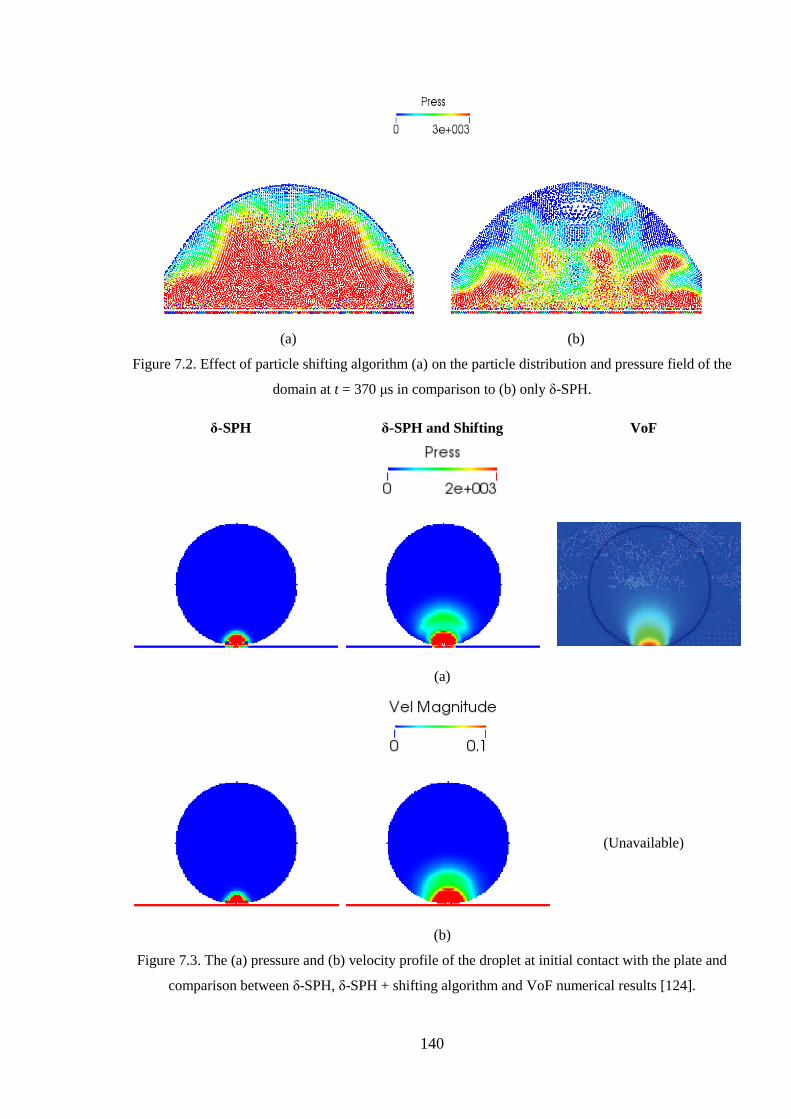
140

(a) (b)

Figure 7.2. Effect of particle shifting algorithm (a) on the particle distribution and pressure field of the

domain at t = 370 μs in comparison to (b) only δ-SPH.

δ-SPH δ-SPH and Shifting VoF

(a)

(Unavailable)

(b)

Figure 7.3. The (a) pressure and (b) velocity profile of the droplet at initial contact with the plate and

comparison between δ-SPH, δ-SPH + shifting algorithm and VoF numerical results [124].

141

The void structure of Figure 7.2 (b) is created due to particles following the streamlines after

a sudden impact of the droplet to the plate creating particle line structures (stacks of particle

lines following the streamline) that eventually collapse after particle clumping has occurred.

This unphysical void and particle clumping phenomena disturbs the pressure field either by a

spurious pressure field or by pressure waves originating around the void. This can be clearly

observed in the comparison of Shepard and δ-SPH density correction of Figure 7.1(c) where

an oval shape high pressure area near the top of the droplet is created that is finally

manifested as voids at later time in Figure 7.2 (b). In addition to the void formation effect of

shifting, the pressure field of Figure 7.2 (a) is considerably smoother and symmetric. Since

the surface shifting of Lind et al. [117] is employed the surface of Figure 7.2 (a) is smooth

maintaining an angular shape.

However, since particles are shifted from their original position based on Fick’s law, at

impact – keeping in mind that in WCSPH small compressions of the order of 1-2% are

permitted through the equation of state and the numerical speed of sound – the compressed

particles should in theory shift from the high concentration impact zone to the lower

concentration interior droplet domain.

This redistribution of particles from the high to the low pressure zone will alter the pressure

field in the droplet transmitting the pressure wave and therefore reducing the compressibility

of the fluid. Evidence of this assumption is given in Figure 7.3 where a comparison of the

pressure field with and without δ-SPH and a Volume-of-Fluid (VoF) simulation is shown

[124].

However, the shifting algorithm may introduce some numerical diffusion to the simulation

since particles are shifted numerically to different positions. A measure of the minimum

numerical diffusion is given in Equation (5.22) using the minimum particle Peclet number.

For a convection velocity of umax = 2 m/s and assuming the maximum concentration gradient

change is located at the free-surface curvature of the droplet the minimum particle Peclet

number is Pemin = 40 which can be interpreted as a convection dominated flow.

Next, a well known SPH validation case is used to access the viscous forces formulation, δ-

SPH and shifting algorithm in the liquid phase using a dam break.

142

7.2.1.2. Dam break validation

To demonstrate the validity of the liquid phase, the dam break test case has been chosen. The

dam break case is a typical SPH validation case for gravity – pressure driven flows with non-

linear free surfaces.

In line with available experimental data [105], a container with a length of 4L and height of

3L contains a column of water with height H = 2L and length L = 1 m. The water column is

located in the left hand side supported by a gate which is suddenly removed to start the water

column collapse. The liquid impinges on the right hand side wall with an impact pressure

increase and fragmentation of the free surface. A schematic of the dam break test case in

given in Figure 7.4. An initial particle spacing of dx = 0.01 m produced 22 000 particles.

Figure 7.4. Schematic of the dam break test case with L = 1 m.

The liquid is considered as water with a density of ρ = 1000 kg/m3 and a dynamic viscosity of

μ = 10-3

Pa s. The δ-SPH diffusion coefficient was 0.1 which is typical for such simulations

[145] with a shifting parameter of A = 2. The numerical results are compared with the

experimental results of Koshizuka and Oka [105]. Figure 7.5 and Figure 7.6 show the water

toe advance and height reduction as the dam breaks to the right hand side in non-dimensional

form by

L

hh

L

xx

L

gtt

2*,*,

2* , (7.1)

where t, x and h is the time toe position and water height respectively.

143

Figure 7.5. Dam break toe front comparison between the experimental and numerical results for a

particle spacing dx = 0.01 m.

Figure 7.6. Dam break height (height decrease of the water column as the dam breaks) comparison

between the experimental and numerical results for a particle spacing dx = 0.01 m.

144

Both figures show close agreement with the experimental results with small variations of the

water height reduction after t* = 4, which is known to be associated with the dynamic

boundary conditions and particle sticking effects that are associated with the current

boundary condition. Nevertheless the agreement is satisfactory. Since the dam is breaking

progressively due to gravity and the impact pressure field is similar in both cases and is not

included in this work.

Next, the saturated sediment phase is examined for a number of test cases in terms of the

yield criteria, the pressures of the two-phase model (i.e. mixture and skeleton pressure) and

the validity of the constitutive equations.

Partial summary

In Section 7.2.1 the predictive accuracy of the fluid was examined for gravity and pressure

driven flows. The droplet impacting a flat plate case has been employed to demonstrate the

effectiveness of the δ-SPH algorithm through the dissipation term included in the continuity

equation under violent impact flows in comparison to the Shepard filter. However, care must

be taken when choosing the diffusive coefficient of δ-SPH that may result in over dissipation

of the density field. Another essential implementation to the liquid phase was the particle

shifting algorithm.

Particle shifting is used in this thesis to stabilise the computation by smoothing the particle

distribution from high to low concentration areas of the domain and reduce the void

structures created due to particles following the streamlines after a sudden impact of the

droplet to the plate creating particle line structures. It has been demonstrated that the

unphysical voids are dissipated with a smoother pressure field.

To validate the shifting and δ-SPH algorithm implementation, a dam break test case has been

used. The toe advance and height reduction of the dam as it breaks were in good agreement

with experimental data. Small deviations from the experimental data in the height of the

water column were due to the boundary conditions and the reader is referred to Chapter 8.

7.2.2. Sediment phase

7.2.2.1. Yield criteria validation using Kanatani’s approach

Kanatani [100] reduced the Drucker-Prager model to an associated flow rule for

incompressible sediment flows to the expression of Equation (5.45)

145

capy . (7.2)

Herein, a similar approach has been used as described in Section 5.3.1 by using the

Newtonian constitutive equation written in the following form

Ddy II 2 , (7.3)

or

max2

D

yapp

II, (7.4)

where μapp

is the apparent viscosity of the sediment under yielded conditions and μmax

is the

sediment viscosity before yielding μs. This simplistic methodology of describing the sediment

flow behaviour has proven effective by other researchers in SPH [57, 138, 195] and is being

investigated herein in terms of the suitability of two effective stress yield criteria models. A

comparison between the Mohr-Coulomb (MC) and Drucker-Prager (DP) yield models is

given below for static and dynamic cases with qualitative and quantitative comparisons with

analytical solutions and experimental results.

However, more complex constitutive equations have been used in this thesis, already

discussed in Section 5.3.2.3, and the purpose of this Section is to show the applicability of the

yield criteria and yield surface prediction.

Still sediment-liquid case

A variant of the still water test case which is a typical SPH validation case has been used to

assess the interface of the two phases, the variable viscosity and density in the sediment and

liquid. The sediment is located at the bottom of a tank with the liquid phase above at the top

in a 2-D case where the length and height of the tank is L = 4.0 m and the height of the solid

sediment is Hs = 1.0 m with equal liquid height Hl = 1.0 m as shown in Figure 7.7.

Three different particle spacing configurations have been used to demonstrate the

convergence of the case. The particle spacing is varied from dx = 0.04 m to dx = 0.01 m

resulting in 1446, 5391 and 9500 particles respectively.

The liquid reference density was set to ρl = 1000 kg/m3 with the saturated sediment reference

density equal to ρs = 1750 kg/m3 following the relationship ρs = 1.75 ρl. The dynamic

viscosity of liquid was set to µl = 10-3

Pa s and the sediment maximum viscosity was set to µs

= 5 103 Pa s with the Coulomb parameters c =1000 Pa and = 45˚. The still sediment-liquid

146

case was initialized to the reference density conditions of ρs = 1.75ρl for the for the liquid

and saturated sediment density.

Figure 7.7. Definition sketch of the domain for the still sediment liquid case.

A convergence analysis based on the Global Relative Error (GRE) which can be used as a

measure of the stillness of the sediment after yielding [163] has been performed according to

N

jn

i

n

i

n

i

x

xxGRE

21

, (7.5)

where x is the position of the particle and n denotes the time step.

The motivation at this point is to assess the stability of the interface between the sediment and

the liquid when, in theory, there should be no movement. However, in SPH small tiny

movements of particles always occur, hence, this case tests the stability of the yield models

embedded within SPH at the interface. Figure 7.8 shows the convergence of the still case

using both yield criteria, at different particle spacing. In addition, a steady state threshold

(GRE < 10-5

) has been introduced below which the particles of both phases are said to remain

still.

It is shown that below a particle spacing dx = 0.02 m initially the GRE increases above the

threshold as would be expected caused by the relative movement of the liquid particles due to

the SPH error. After t = 0.6 s a steady state has been reached. The rearrangement of liquid

particles is reduced over time and the simulation returns to steady state. For a particle spacing

of dx = 0.04 m the GRE remains above the threshold value for both models.

147

Figure 7.8. Comparison of the Mohr-Coulomb (MC) and Drucker-Prager (DP) yield criteria for

different particle spacing using the GRE over time.

The GRE for the MC and DP models appears similar for the fine particle spacing with the

exception of some peak values at around t = 0.4 s where the MC exhibits small oscillations.

Therefore, a ratio of dx / h = 0.769 is necessary for a steady state interface based on a kernel

smoothing length of as = 1.3 and particle spacing dx = 0.02.

Figure 7.9 shows the viscosity of the still liquid-sediment phase for both models at t = 0.2 s

with a particle spacing of dx = 0.01 m. Notable is the difference of the yield surface thickness

of the two models across the mid-depth of the tank in Figure 7.9. Note that at this instant (t =

0.2 s) both models exhibit almost the same degree of stillness and hence value of GRE, but

the actual yielded surface is different. The DP criterion tends to have a larger yielding

interface creating a thicker shear layer between the liquid and the sediment in comparison to

the shear layer resulting from the MC criterion. This result appears to be in agreement with

the other test cases examined later.

The advantage of this test case is that it illustrates the stability at the interface. The interface

remains steady without particle exchange, diffusion or unphysical repulsion. The variable

viscosity remains close to the threshold with low or little variations when steady state is

reached with the exception of the interaction with the boundaries where small variations

occur when the GRE is above the threshold level which is expected.

148

(a) (b)

Figure 7.9. Viscosity of the still liquid-sediment phase for (a) Mohr-Coulomb (MC) and (b) Drucker-

Prager (DP) yield criterion at t = 0.2 s.

Tangential annular flow between two coaxial rotating cylinders

The tangential annular flow test case has been applied to validate the rheological parameters

of the sediment-liquid mixture. In this shear driven test case, two co-axial cylinders with

radius R1 = 0.5 m and R2 = 0.1 m are co-rotating at a steady frequency of f = 5 Hz as shown in

Figure 7.10. To avoid initial sudden disturbances at the start of the simulation the velocity of

the cylinders walls is linearly accelerated to their terminal viscosity over a period of t = 0.1 s.

Figure 7.10. Definition sketch of the domain for the tangential annular flow between two coaxial

rotating cylinders.

The sediment mixture density is set to ρs = 1540 kg/m3 with a viscosity of 1000 Pa s and the

Coulomb parameters c = 100 Pa and = 45°. The total number of sediment particles is 3703

with a particle spacing of dx = 0.02 m.

In 2-D, assuming that the flow is laminar and incompressible at steady state, only the

tangential velocity is non zero with no pressure gradient in the circumferential direction, the

velocity profile can be found as [18]

149

r

CrCu 21

2

, (7.6)

where C1 and C2 are the integration constants.

An L2 error for the velocity u can now be defined as

N

j

SPHanalytical

u

uu

NuL

2

max2

1)(

. (7.7)

Figure 7.11 shows the L2 error for both yield criteria against time. The L2 error levels for both

cases show a steady convergence within acceptable levels. Apparent is the slow decay in L2

error of the DP criterion, in agreement with the still sediment liquid case, whereas the M-C

criterion reached steady state faster.

The physical meaning of the slow L2 error decay is that the sediment flow is much less

viscous in comparison with the MC criterion. Therefore the shear flow induced by the axial

boundaries reduced the variable sediment viscosity further than the MC criterion, taking more

time to reach steady state. Both yield criteria finally reach the same L2 error at steady state at

the end of the simulation. Figure 7.12 shows a graphical representation of the velocity

distribution after 1 revolution (0.2 sec) and at 10 revolutions (2.0 sec). Note that the DP

criterion, evident also by the L2 error, at 1 revolution has not reached steady state.

Figure 7.11. Temporal growth of L2 error for the Mohr-Coulomb and Drucker-Prager yield criteria for

a tangential annular flow.

150

(a) MC (b) DP (c) MC (d) DP

Figure 7.12. Velocity distribution of the sediment after 1 revolution (a & b) and at the end of the

simulation (c & d) after 10 revolutions.

Two-phase tangential annular flow

The tangential annular flow test case has been extended to a two-phase case to investigate the

sediment and liquid rheology and interface. The geometrical configuration of the case is

identical to the single phase case. However, the outer half of the interior domain of the

annulus is filled with sediment particles and the inner with liquid particles.

The liquid and sediment particle spacing and properties are as follows. The particle spacing is

set to dx = 0.0039 m that resulted in 50 886 particles. The liquid reference density is set to ρl

= 1000 kg/m3 with the sediment reference density equal to ρs = 1.54 ρl. The viscosity of the

liquid is set to µl = 10-3

Pa s. Two different values of sediment viscosity have been used with

μs = 5 103 Pa s and µs = 1 Pa s which is considerably lower. The reason for the second lower

viscosity is to test the stability of the behaviour of the interface and investigate the effect on

the flow reaching steady state. Since the maximum apparent viscosity is three orders of

magnitude lower that the single phase tangential annular flow, both yield criteria should

behave in a similar manner. At steady state a uniform axial particle distribution should be

observed.

Figure 7.13 shows the L2 error for both yield criteria against time. The L2 error provides a

measure of steady state convergence over time. Both yield criteria finally reach the same L2

error at steady state at t = 1.2 s. As expected the difference between the two models is

minimal for the low viscosity and behaves similar to the single phase for the higher viscosity.

In addition a qualitative comparison of the flow field is given in Figure 7.14.

151

(a)

(b)

Figure 7.13. The growth of L2 error for the MC and DP yield criteria for a tangential annular flow for

μs = 5000 Pa s and μs = 1.0 Pa s.

152

MC, μs = 1.0 Pa s

DP, μs = 1.0 Pa s

(a) (b)

MC, μs = 5000 Pa s

DP, μs = 5000 Pa s

(c) (d)

Figure 7.14. Velocity field after 2.5 revolutions for the MC with (a) μs = 1.0 Pa s, (c) μs = 5000 Pa s

and the DP with (b) μs = 1.0 Pa s, (d) μs = 5000 Pa s.

The last two cases demonstrate not only the convergence of the L2 error within acceptable

levels and the difference between the Mohr-Coulomb and Drucker-Prager models but in

addition, the importance of the sediment viscosity value μs. Using Kanatani’s approach to

acquire a μapp with a maximum threshold viscosity μs may result in an under estimation of

scouring for high values of μs that have been traditional used to avoid creeping [57, 138, 195]

but low values will result in over estimation of the scouring phenomenon as proven herein.

Nevertheless both yield criteria produce satisfactory results. It is evident from the still

sediment-liquid, the tangential annular flow and the current test case that the MC criterion

tends to reduce the shear layer by means of higher variable viscosities when the sediment

153

particles are suspended trending to a more conservative model which underestimates the

erosion profile. The MC criterion may underestimate the yield strength of sediment [99, 218]

which is in line with this discussion, whereas, the DP criterion is said to be a smoother

alternative to the MC criterion where the yield strength, at least on these specific test cases, is

better depicted.

Next, a dynamic scouring test case is examined by using an erodible dam break to evaluate

the scouring profile and shear layer with available experimental results.

2-D Erodible dam break

The shear layer and suspension of the sediment is qualitatively validated using an

experimental erodible dam break [65]. When the liquid column is released, the hydrodynamic

stress at the interface induces scouring at the sediment interface. The shear layer induced

propagates to some depth where the viscosity, density and pressure changes from their

initialized value.

In the computational setup a fully saturated sediment bed with height Hs = 0.6 m is located

below a dam of liquid with height Hl = 0.1 m and length Ll = 2.0 m. A definition sketch is

shown in Figure 7.15. The particle spacing is set to dx = 0.002 m producing 328 353 particles

in the domain. The density ratio between the two phases is ρs = 1.54 ρl with the liquid density

ρl = 1000 kg/m3. The sediment and liquid viscosity was set to µs = 1000 Pa s and µl = 10

-3 Pa

s respectively. The sediment Coulomb parameters are set to c = 100 Pa and = 45˚ (in line

with Ulrich et al. [196]).

Figure 7.15. Definition sketch for the 2-D erodible dam break configuration.

Figure 7.16 to Figure 7.19 shows a comparison of the shear layer velocities within the

suspension layer of the sediment and compares the experimental results from the Louvain

experiment [65] with the MC and DP yield criteria for different points in time of the

simulation (at t of 0.25 s, 0.50 s and 1.00 s).

154

Comparing the two yield criteria the DP yield model shows better agreement in the sediment

shear layer with the experimental results. The MC criterion appears to under predict the

erosion and the depth of the shear layer. The erosion of the shear layer with the DP model is

more distinct with larger depths. In addition, the dunes created by the liquid in the shear layer

agree closely with the shape from the experimental results. Also, the liquid peak at the free

surface is in closer agreement with the DP criterion. For example the liquid surface peak

created by the scoured sediment is dominant in the experimental results and DP criterion for t

= 1.0 s but absent at the MC model (Figure 7.19).

Ex

per

imen

tal

(a)

MC

(b)

DP

(c)

Figure 7.16. Shear layer formation and shear layer velocity field for the Mohr-Coulomb (a) and the

Drucker-Prager yield criterion at t = 0.25 s and qualitative comparison with the experimental results,

not in the same horizontal scale [65].

155

Figure 7.16 shows a snapshot of the experimental and numerical results at t = 0.25 s. It can be

clearly observed that the shear layer produced by the DP criterion tends to be thicker with the

sediment being transported along after the dam breaks onto the sediment. The shape of the

wave front is more closely related to the DP model in comparison with the experimental

results. Nevertheless, the MC model shows reasonable agreement with the experimental

results.

Ex

per

imen

tal

(a)

MC

(b)

DP

(c)


Drucker-Prager yield criterion at t = 0. 50 s and qualitative comparison with the experimental results,


156

In Figure 7.17 the dam front has advanced forward eroding the sediment surface. However

the initial dune created by the dam break at t = 0.25 s is well defined in the experimental

results. Also, the liquid motion creates a thick shear layer at the interface. These

characteristics tend to be in agreement with the DP rather than the MC model. E

xp

erim

enta

l

(a)

MC

(b)

DP

(c)


Drucker-Prager yield criterion at t = 0.75 s and qualitative comparison with the experimental results,


In line with the previous discussion, Figure 7.18 and Figure 7.19 follow similar behaviour.

However, at t = 0.75 s and t = 1.0 s the liquid free surface peak just after the scoured area of

the initial dam break impact to the sediment bed is well defined in the experimental results.

157

Hence, the kinematics of the liquid have changed by the influence of the bed profile and

scouring behaviour. As with before the agreement with the DP is closer.

Ex

per

imen

tal

(a)

MC

(b)

DP

(c)


Drucker-Prager yield criterion at t = 1.0 s and qualitative comparison with the experimental results

[65].

Since the qualitative results have demonstrated that the initial dam break impact at t = 0.25 s

can influence the kinematics not only of the shear layer but the liquid kinematics a more

detailed comparison is shown in Figure 7.20. Both yield models tend to be in good agreement

with the experiment but at least in this experiment the DP appears to capture the experimental

trend closely.

158

Figure 7.20. Dam break profile at t = 0.25 s for the MC and the DP criterion against the experimental

data.

Partial summary

In this Section, a comparison of the suitability of two effective stress yield criteria models has

been performed for static and dynamic cases with qualitative and quantitative comparisons

with analytical solutions and experimental results. The surface yielding of the sediment was

modelled by modifying the Newtonian constitutive equation to include yielding at the

interface of the phases and a variable sediment viscosity for modelling the dynamics of the

sediment. This approach is based on the infinitesimal rate of deformation of the material as a

ratio between the yield stress and the sediment deformation.

In the cases examined small improvements were observed by the Drucker-Prager model. It

has been shown that the bed profile and scour behaviour influences the kinematics not only of

the sediment phase and the scour profile induced by the liquid, but also the liquid behaviour

itself with the creation of dunes and scour holes changing the kinematics of the liquid

considerably. Nevertheless, for a perfectly plastic frictional material prior knowledge of the

behaviour of the material and the hydrodynamic application should be known.

159

7.2.2.2. Validation of Bingham constitutive models

Sediment block collapse

Numerical simulations are conducted to simulate experiments of Lube et al. [132] for

granular flows. Lube et al. [132] investigated granular flow patterns of granular material

block collapses under gravity. Such test cases serve validation purposes for the sediment

single phase model and its rheological characteristics.

In the experiments, a vertical 3-D axisymmetric column of dry sand collapses under

gravitational force with the flow behaviour depending on the aspect ratio of

c

cr

r

ha , (7.8)

where hc and rc is the height and radius of the column respectively. Lube et al. [132]

conducted a number of experiments for different aspect ratios and proposed a best fit

equation based on the experimental results for ar < 1.7,

7.124.1 aforar

rr

c

c, (7.9)

where r∞ is the run-out distance measured form the centre of the column.

Herein, the more challenging low aspect ratio of ar = 0.55 is chosen to validate the granular

flow model as outlined by Chen et al. [38]. A vertical 2-D column with dimensions rc = 0.1

m and hc = 0.055 m has been chosen from the experimental results pool. The initial particle

spacing was set to 0.001 resulting in 12 000 particles. The density of the simulated sand was

2600 kg/m3 with the Coulomb parameters set = 30˚ without cohesion (c = 0 Pa).

Since the granular material is dry, a Bingham model has been used and therefore the

Herschel-Bulkley-Papanastasiou model was reduced to a Bingham model by setting the

exponential growth of stress m to 0 and the power law index n to 1. To address the

discontinuity associated with the Bingham model as IID → 0, a maximum yield stress is used

with τy = 2000 Pa which is representative of such flows [86, 195].

Figure 7.21 shows the accumulated τy and Figure 7.22 the pressure field for the collapsing

sand column. Notable are areas at the top of the column of the yield strength and pressure

where accumulation of yield strength has occurred either by creeping or particle stacking

similar to Section 7.2.1 since the sediment phase does not include the shifting algorithm.

160

Figure 7.21. Yield strength of the sediment at rest.

Figure 7.22. Pressure field after the soil column collapse.

Figure 7.23. Results reported from Chen et al. [38] for the soil column collapse case.

In addition results reported by to Chen et al. [38] using a non-associated flow rule are shown

in Figure 7.23. The run-out distance comparison between the current and Chen et al. [38]

model are in agreement to the equation of Lube et al. [132] predicting an run-out distance of

161

0.168 m which is the same as the numerical run-out distance. The profile of the experimental

and numerical profile for the collapsing column of sediment is shown in Figure 7.24.

Figure 7.24. Comparison of experimental [132] and SPH numerical profile of the collapsing sand

column.

The numerical profile is in good agreement with the experimental data with a deviation near

the boundary. The divergence from the experimental results near the boundary is mainly due

to the dynamic boundary conditions used in this work and is being discussed further in

Section 8. However, small departures are also observed at the top of the column.

Nevertheless, the agreement is satisfactory.

Sediment Dam Break

Bui et al. [26] conducted 2-D dam break experiments with aluminium bars to validate the

numerical solution of a non-associative flow rule model based on the Drucker-Prager

criterion and reported results on the profile of the dam after collapse but most importantly the

failure area of the sediment dam which was unavailable in the sediment block collapse. In the

experimental setup aluminium bars with a diameter of 0.001 m and 0.0015 m and length of

0.05 m where used to simulate 2-D conditions. In the numerical experiment, equal number of

experimental aluminium bars and particles has been used with an initial particle spacing of

0.002 m resulting in 5000 particles resulting in one-to-one simulation. The dam dimensions

were L = 0.2 m and H = 0.1 m with a density of ρ = 2650 kg/m3. The friction angle was to be

= 19.8˚ on a non-cohesive material.

162

(a)

(b)

(c)

Figure 7.25. Dam break comparison between: (a) the experimental results of Bui et al. [26], (b)

numerical results of Bui et al. [26] with the yield surface and (c) results of the current numerical

model and comparison of the experimental profile and yielded surface of the aluminium bars, black

dots denote free-surface and red dots yield surface profile.

163

Figure 7.25 shows a comparison between the experimental and numerical results of Bui et al.

[26] and the results of the current model including the surface profile and yielded area

comparison with the experimental results. The agreement of the dam break surface is

satisfactory with the exemption of the run-off area of the dam break toe. Also, the yield

surface shows good agreement with the experimental data and the numerical results of Bui et

al. [26]. The issue on the run-off toe was identified in the collapsing sand box experiment and

is associated with poor boundary conditions. This is clearly identified in the pressure field of

Figure 7.26. The toe front of the dam seems to have high pressure at the front with spurious

pressure field near the run-off area. Finer resolution simulations reduced the error but the

spurious pressure field near the run-off area was still present.

Similar issues have been identified by other researchers using the dynamic boundary

conditions of DualSPHysics in multi-phase simulations [144].

Figure 7.26. Pressure field of the collapsing dam break, note the poor pressure prediction at the toe

front, black dots denote free-surface and red dots yield surface profile.

Concluding, the comparison of the numerical experiment with the available results from Bui

et al. [26] were in close agreement for the dam break surface and the yielded region. Small

departures have been observed on the dam break toe which is mainly associated with the

boundary conditions used in DualSPHysics.

164

Erodible dam break

The erodible dam break of Section 7.2.2.1 is re-examined using the multi-phase model

implementation of Section 5.3 but using the Herschel-Bulkley-Papanastasiou constitutive

equation and suspension model.

The geometrical characteristics and particle spacing is identical to the erodible dam break of

Section 7.2.2.1. The density ratio between the two phases is ρs = 1.54 ρl as previously but the

viscosity and Coulomb parameters slightly modified to allow a direct comparison with results

obtained by the experiments and Ulrich et al. [195]. Hence, the sediment and liquid viscosity

was set to µs = 500 Pa s and µl = 10-3

Pa s respectively and the sediment Coulomb parameters

were set to c = 0 Pa and = 31˚. The Herschel-Bulkley-Papanastasiou parameters of

exponential growth of stress and power law index were set to m = 10 and n = 0.4

respectively.

Figure 7.27 to Figure 7.30 show a qualitative comparison of the experimental profile and the

numerical results. Also, a quantitative comparison has been performed using the experimental

results, the results reported by Ulrich et al. [195] and the current model for the profiles of the

liquid and sediment. The main difference with the Ulrich et al. [195] model is the treatment

of the sediment phase by different yield criteria and constitutive equation (see Section 2.7.2).

(a)

(b)

(c)

Figure 7.27. Qualitative comparison of (a) experimental [65] and (b) current numerical results and (c)

comparison of liquid-sediment profiles of the experiments, numerical results of Ulrich et al. [195] and

current model at t = 0.25 s.

165

(a)

(b)

(c)




(a)

(b)

(c)




166

(a)

(b)

(c)




Figure 7.27 shows the liquid and sediment profile at t = 0.25 s which follows the initial dam

release. The profile of the experiment seems to be in good agreement to the numerical profile

and follows similar trend at the liquid surface and the interface between the liquid and the soil

mixture. As small departure is visible at the toe front of the dam were the numerical model

run off distance is marginally forward of the experimental. Nevertheless, comparing the

numerical profile with the numerical results of Ulrich et al. [195] demonstrates that the model

of Ulrich et al. under predict the scouring profile at x = 0.0 m and the creation of a dune at x

= 0.1 m considerably and therefore the liquid surface peak around that area of the dam toe

front.

This underprediction of the liquid surface peak and scour profile is also visible in Figure 7.28

where Ulrich et al. reported minimal scouring at the interface. However, even if the current

model follows the scouring profile trend of the experiments at t = 0.50 s it over predicts the

interfacial profile. However, the liquid surface is well represented.

This over prediction of scouring is present at t = 0.75 s and t = 1.00 s in Figure 7.29 and

Figure 7.30, moreover the current numerical profile is in better agreement to the numerical

model of Ulrich et al.

167

Concluding, the Ulrich et al. [195] and the current numerical model compared herein

preformed reasonably well reproducing closely the hydrodynamics and scouring process.

However, the profile trend of the current model appears to follow the liquid surface and

interface profile closer. The scouring profile was slightly over estimated in the current model

at t = 0.5 s and it is believed to be linked with the shear thinning parameter of the Herschel-

Bulkley-Papanastasiou model. The tuning parameters of constitutive equations such as the

current, the GVF or more advanced models has been reported to be a drawback since it is

difficult to [35, 38, 176] determine experimentally.

Note that the issues identified earlier with the boundary conditions employed in

DualSPHysics were not present in this test case since the kinematics of the flow were mainly

associated with the interface.

Partial conclusions

In Section 7.2.2.2, validation cases have been presented for dry and saturated sediment under

gravity, pressure and liquid induced flow. The sediment block collapse showed good

agreement with the experimental profile and similar behaviour to other numerical models.

However, accumulated yield strength was present in some streamlines of the soil. These

streamlines were symmetrical similar to the streamlines present in the liquid phase when

shifting was not employed. Therefore a second test case has been presented. The soil dam

break showed good agreement with the profile of the experiments but most importantly the

agreement of the numerical yield surface and the experimental was satisfactory. The erodible

dam break was revisited using a more elaborate constitutive equation. The agreement with the

experiments was reasonable and the model showed some improvements over similar

numerical models. However, at some points some over prediction of the scour profile

occurred.

Next, a liquid-sediment 3-D case is presented. The 3-D case has served as a benchmark case

for validating sallow water equation models in the past and to the authors best knowledge this

is the first time this test case has been performed in SPH.

168

7.3. 3-D validation case

7.3.1. 3-D erodible dam break

In this Section, the numerical results for a 3-D validation case are presented. The

experimental test case of Soares-Frazão et al. [186] provides validation data for numerical

models for dam-break simulations over mobile beds with fast transient flows involving

sediment transport. Initially, the test case was set as a benchmark blind test to the scientific

community with twelve modelling teams participating.

Figure 7.31. Schematic of the 3-D dam break experiment.

In the experiments a 27 m long flume is used where the breached dam is represented by two

impervious blocks with a 1 m wide gate located between the blocks. Figure 7.31 shows a

schematic of the experiment. The height of the sediment was 0.085 m located 1.5 m before

the gate and extended to over 9.5 m as shown by the hatched area of Figure 7.31. The

sediment had a uniform coarseness with a sediment to fluid density ratio of 2.63 and a

porosity of nr = 0.42. The fluid height in the reservoir was 0.470 m for the current experiment

case.

Two measuring points US1 and US6 were used to measure the water levels and three bed

profiles were taken at y1, y2 and y3 at the end of the simulation at t = 20 s (Figure 7.31).

In the numerical model the particle spacing was set to 0.005 m resulting in 4 million particles

of which 701132 were boundary particles. The initial density of the fluid and sediment was

169

set to hydrostatic and lithostatic conditions, respectively. The δ-SPH parameter for this

simulation was set to 0.1 as recommended in [145]. The fluid dynamic viscosity was 0.001

Pa s and sediment viscosity was set to 150 Pa s with the HBP m and n parameter set to 100

and 1.8 respectively. The value for the exponential growth m parameter value was chosen to

approximate a Bingham model as closely as possible with a minimal pseudo-Newtonian

region and the power-law exponent n to resemble shear thinning materials as shown in Figure

5.8.

Finally a small amount of cohesion was given to the sediment phase of c = 100 Pa to stabilise

the interface and control the scouring near the dam gate. Next, the water level height and

sediment profiles are presented against the experimental data for the aforementioned control

points.

7.3.1.1. Sediment bed profiles

The sediment profile in comparison with the experimental data is shown in Figure 7.32 for

three different cross-sections of the sediment bed at locations y1, y2 and y3. The numerical

results are compared with four different runs (labelled as b1, b2, b3 and b4) of the experiment

as reported by Soares-Frazão et al. [186] with the SPH data superimposed on the

experimental data. The data from runs b1 –b3 show the variability in the experimental data.

The bed profile at y1 shows satisfactory agreement with the experimental results for most of

the length of the bed. Some deviations from the experiment are notable specifically near the

dam break gate around x = 0.5 m to x = 1.5 m. Nevertheless, looking at the experimental

results there is a disagreement on the repeatability of the experimental results with some of

the runs having lower scouring at the front with a peak for runs b and d whereas the

numerical results are in better agreement with runs a and c.

Also a small deviation is observed at x = 4.0 m where the numerical model over predicts the

scouring region. At y2, the agreement is marginally better from y1 with only small deviations

near the wall at x = 0.5 m which were expected due to the boundary conditions implemented

in DualSPHysics that exhibit a sticking behaviour near the walls. Finally, the y3 bed profile

shows similar problems near the wall over predicting the sediment height. Also, the sediment

peak is slightly under predicted with a small delay on the location of the peak.

170

(a)

(b)

(c)

Figure 7.32. Repeatability of the bed profiles at locations (a) y1, (b) y2 and (c) y3 of the experiment and

comparison with the numerical results.

171

However, due to the complexity of the 3-D dam break case the sediment profiles are

satisfactory since the hydrodynamics of the fluid are very complex especially at the gate with

a rarefaction wave and a initial hydraulic jump. Unfortunately, results of the upstream flow or

near the gate are not reported in Soares-Frazão et al. [186]. A snapshot of the velocities of the

sediment from the numerical experiment is shown in Figure 7.33 and the profile of the bed is

shown in Figure 7.34.

Figure 7.33. Velocity magnitude profile of the bed at t = 20 s.

Figure 7.34. Height profile of the sediment at t = 20 s.

172

7.3.1.2. Water level measurements

The hydrodynamics of the flow are linked to the sediment scour mechanisms. In this section,

two water level probes locations are used to measure the numerical water levels and compare

with the experimental results of the 3-D dam break. The experimental profiles for gauge US1

and US6 shown in Figure 7.31 are compared with the numerical run.

(a)

(b)

Figure 7.35. Repeatability of the water level measurements of the experiment for gauge US1 and US6

and comparison with the numerical results.

173

The water height levels of gauge US1 which is located near the gate shows reasonable

agreement with the reported experimental results with a small over prediction at the end of

the simulation. Similar results are shown for gauge US6 with the exception of a sudden drop

in water level at t = 3.0 s. We suspect the water level deviation at this point is an error in

numerical sampling and is under further investigation. Another explanation might be an

absence of fluid particles in the sampling control volume since we are using sparse sampling

times of 1 s. Both graphs show slightly over predicted water heights particularly at location

US6. This is in agreement with the sediment profiles which show a small bed thickness over

prediction downstream.

Concluding, the results from the numerical experiment of a 3-D dam break have been

compared with a benchmark dam break case of Soares-Frazão et al. [186]. To the authors

best knowledge this is the first time this test case has been performed in SPH mainly due to

the large domain and therefore the high computational cost. The 3-D erodible dam break took

14 days on a Tesla K20 GPU card for 4 million particles.

The 3-D dam break bed profiles of the sediment located at the bottom of the tank were

satisfactory reproduced in this numerical experiment with only small deviations near the gate

and a small over prediction downstream that might be accounted for by the departure in the

dynamics of the fluid. Also the water level profiles at two discrete locations have been

presented with reasonable agreement to the experimental results.

7.4. Concluding Remarks

In this Chapter a number of test cases have been presented to validate and verify the

capability of the model presented in Chapter 5 using the GPU implementation of Chapter 6.

The test cases have been chosen for their simplicity and available analytical or experimental

data. In addition, some of the validation cases have been used in the past by other SPH

practitioners and therefore a direct comparison of the numerical models that reveal the

advantages and disadvantages of each model can be easily identified.

Both phases have been validated targeting the proposed modifications such as the liquid

phase and the droplet test case which yield interesting conclusions on the use of δ-SPh and

the shifting algorithm. The pressure field of the droplet using the shifting algorithm changed

the pressure of the droplet at impact significantly and was in agreement in comparison to

other numerical methods (Volume-of-Fluid).

174

The sediment phase was validated using a single and two-phase flow under gravity and

pressure fields and liquid-driven scour. Two different approaches where demonstrated using

different constitutive equations. The first used the ratio of the yield stress and the strain rate

of the sediment mixture which is a traditional approach in SPH, whereas the second applied a

constitutive equation proposed by Herschel-Bulkley-Papanastasiou. The HBP model

resembles a Bingham model but allows for control on the stress growth and low strain states

and can be tuned to model shear thinning or thickening materials. This Bingham model was

applied to a 2-D and 3-D validation case with significant agreement to the available data.

Observed disadvantages are mainly inherent not only to the model but the SPH method itself.

In both phases a discrepancy near the boundary has been observed. Near the wall boundary

departures from reference data were obvious. The wall boundary conditions used in

DualSPHysics have been known to cause large separation regions with unphysical pressure

fields. In Chapter 8, presents a new improved wall boundary conditions with considerable

success in 2-D and 3-D. On the other hand the two-phase model showed slight over

prediction of the scouring characteristics in the 2-D and 3-D cases. However, the

hydrodynamics of the flow dictate the amount of scouring and the resulting interfacial profile

that may be challenging to predict at the interface. Nevertheless, the free surface of the liquid

and scouring profile was in good agreement with the available reference data.

Chapter 8

8. A new wall boundary condition

8.1. Introduction

Due to the intrinsic nature of kernel based interpolation and to the Lagrangian approach,

imposing boundary conditions in SPH is still an open problem. The approach proposed by

Monaghan [147, 152] is the repulsive force method; where the wall is described by particles

which exert a repulsive short-range force similar to a Leonard-Jones potential force on fluid

particles.

Mirror or ghost particles as introduced by Randles and Libersky [174] is another widely used

way to describe boundaries in SPH [45, 139]. Kulasegaram et al. [106] proposed a variant of

this method which introduces an additional term in the momentum equation in order to mimic

the effect of the wall. This technique eventually uses an empirical function to approximate

the force originating from variational principles. The idea was further developed in [17, 51,

58]. These methods have the advantage of restoring zero-consistency in the SPH interpolation

but the discretization of complex 3-D geometries and/or multi-phase flows is not

straightforward. In general, the repulsive force method is more flexible because it can be used

to describe complex moving boundaries, but it can introduce a non-physical pressure

oscillation and it does not reduce the effect of kernel truncation near the wall.

Ferrari et al. [59] proposed a local point symmetry (as opposed to ghost particles) method,

called the Virtual Boundary Particle (VBP) technique which is able to discretize arbitrarily

complex geometries without introducing empirical forces. Recently the method was further

enhanced and applied to shallow water equations (SWE) [197]. A more elaborate literature

review is given in Section 2.5.5.

In this thesis, the aforementioned VBP wall boundary method is further enhanced and applied

to the Navier-Stokes in order to ensure approximate zeroth and first-order consistency in

presence of arbitrarily complex boundaries using the WCSPH approach in 2-D and lately in

3-D. However, the method can be applied to the ISPH methodology.

176

In this work, the zeroth and first-order consistency refers to the ability of the scheme to

reproduce a zeroth order polynomial and a linear function, respectively by the SPH

interpolation method. The term “approximate” refers to the discretized form of the SPH

interpolation as the particle spacing dx → 0.

This Chapter firstly addresses the issue of particle inconsistency and kernel truncation near

the boundary. Next, the extended modified virtual boundary particle (eMVBP) wall treatment

is presented for the Navier-Stokes equations in 2-D followed by the numerical results for

static and dynamic cases. However, efficiency and GPU parallelisation is essential in 3-D

simulations. The latter method is extended to 3-D to treat arbitrarily complex geometries by

describing the solid wall using triangles to maximize the efficiency and GPU parallelization.

Approximate zeroth and first order consistency are ensured by using a fully uniform fictitious

particle stencil.

8.2. Particle inconsistency in SPH

8.2.1. Kernel particle consistency

Numerical schemes should be able to reproduce the corresponding physical equations of the

continuum domain in a discrete form. SPH achieves that using a smoothing kernel function

(smoothing kernel or kernel) which dictates the connectivity of the surrounding nodes and the

region of influence for each interpolated particle.

For a scalar function f to be reproduced exactly, f must be smooth and continuous in Ω and

the smoothing length h → 0 resulting in a Dirac delta function

'),'()'()( xxxxx dhff , (8.1)

but since the smoothing length is finite, the integral representation is only an approximation

consistent to the nth

order. The accuracy of the approximation can be demonstrated by

applying a Taylor series expansion of f(x’) around x of Equation (8.1)

h

rOdhWhk

fhf n

n

k

kkkk '

'),'('

!

)(1)(

0

)()()()(

xxxxx

xxxx , (8.2)

with k the order of the derivative. For a function f to be approximated to nth

order accuracy

the following moments must hold [11, 126],

177

0'),'()'(

0'),'()'(

0'),'()'(

1'),'(

2

2

1

0

xxxxxM

xxxxxM

xxxxxM

xxx

dhW

dhW

dhW

dhWM

n

n

, (8.3)

assuming that at the support edge the (k-1)th derivative of the kernel vanishes

0|),'(1)(

S

k hW xx where subscript S denotes the surface of the support. These expressions

form the fundamental conditions for the integral approximation, i.e. the first expression of

Equation (8.3) satisfies a zeroth order polynomial ( cf )(x ) and the second expression of

Equation (8.3) a linear function ( caf xx)( ) exactly. This procedure can be similarly

repeated for the first derivative:

0'),'(')'('

0'),'(')'('

1'),'(')'('

0'),'(''

22

1

0

xxxxxM

xxxxxM

xxxxxM

xxx

dhW

dhW

dhW

dhWM

nn

. (8.4)

In addition, to these conditions the kernel function should also vanish over the surface S of its

region of influence Ω:

0|),'(1)(

S

k hW xx . (8.5)

The purpose of investigating the gradients moments is to introduce a numerical measure of

the scheme to correctly predict gradients (first-order in this paper) without the computation of

the gradients being complicated by physics of the problem or equation sets.

Typically in SPH, only the first derivative is used when dealing with the Navier-Stokes

equations since the second derivative is either expressed as the derivative of the first [123] or

by using a combination of a central differencing scheme for the first derivative and an SPH

interpolation for the second [157].

In a continuous form, in the interior domain away from boundaries and for a uniform

distributed stencil of particles both the zeroth and first order moments of Equations (8.3) and

(11) are satisfied since the support is complete, where the kernel symmetry and

178

),'(),'( hWhW xxxx and kernel gradient asymmetry ),'(),'( ' hWhW xxxx xx

properties of the kernel, also hold. In addition, 0|),'(1)(

S

k hW xx is satisfied. Therefore,

constant and linear functions can be exactly reproduced and the SPH method is said to have

C1 consistency. In discrete form the zeroth and first order moments of the kernel function are

only approximately satisfied.

N

j j

j

j

N

j j

j

j

mhW

mhWM

0),()(

1),(

1

0

xxxxM

xx

, (8.6)

and similarly the moments for the derivative of the kernel can be written as

N

j j

j

jj

N

j j

j

j

mhW

mhW

1),()(

0),(

'

1

'

0

xxxxM

xxM

x

x

, (8.7)

where N is the number of j neighbouring particles within the kernel support, m is mass and ρ

is the density of a fluid particle. For a non-uniform distributed particle stencil, the

discretization becomes exact when h → 0 and N → ∞. The error of a finite h and N has been

investigated by many researchers and is beyond the scope of this paper to further analyse, but

in general it is assumed to be of the order of O ( f (N)-1/2

) [204]. In this work we call

approximate C1 consistent that obtained for the discrete SPH interpolation with no kernel

correction.

8.2.2. Inconsistency of the kernel near the boundary

Near the boundaries, considering SPH approximation in discrete form, the kernel support is

truncated since Equations (8.6) and (8.7) are not satisfied, resulting in errors in the

reproduction of constant and linear functions. Figure 8.1 illustrates the mechanism of a

support domain truncated by a boundary in 1-D.

179

(a) (b)

Figure 8.1. Boundary truncation mechanism for the kernel (a) and its derivative (b) on 1-D space.

To restore approximate consistency near the boundary due to truncation for a uniform particle

distribution Equation (8.6) is rewritten as a summation over interior fluid particles and

particles that represent the boundary

bf

bf

N

Bj j

j

jj

N

Fj j

j

jj

N

Bj j

j

j

N

Fj j

j

j

mhW

mhW

mhW

mhWM

),()(),()(

),(),(

1

0

xxxxxxxxM

xxxx

, (8.8)

and similarly for the derivative, Equation (8.7) becomes

bf

bf

N

Bj j

j

jj

N

Fj j

j

jj

N

Bj j

j

j

N

Fj j

j

j

mhW

mhW

mhW

mhW

),()(),()(

),(),(

'

1

'

0

xxxxxxxxM

xxxxM

xx

xx

, (8.9)

where the Fp represents the set of Nf interior fluid particles and Bp represents the set of Nb

particles representing the boundary. Clearly, for a C1 consistent approximation the interior

and the boundary particles summation are needed near the wall, with the Nb summation

providing the truncated support of the wall.

The Equation of conservation of mass (4.7) in discrete form near the wall boundary can now

be written as

bf N

Bj

ijijj

N

Fj

ijijji WmWm

dt

duu

. (8.10)

180

With the as-yet unspecified boundary particles, the kernel support can be considered

complete, hence the anti-symmetric property of the kernel is not violated and therefore,

conditions of Equation (8.8) and (8.9) are satisfied. Note, that the conservation of mass for a

volume V still holds and integration of the continuity equation (8.10) yields

0dt

dm, (8.11)

at any control volume locally and therefore, the global mass of the system remains unchanged

for a closed system.

Following the same approach, the inviscid momentum Equation (4.17) can be written as

i

N

Bj

ij

ji

ji

j

N

Fj

ij

ji

ji

ji

bf

WPP

mWPP

mdt

dg

u

. (8.12)

Vaughan et al. [204] has demonstrated that the momentum equation can be recovered from

the inviscid discretized form

i

N

j

ij

ji

ji

ji W

PPm

dt

dg

u

, (8.13)

by performing a Taylor series expansion on Pj resulting in

i

N

j

ijiijii

j

j

i

i WPPPm

dt

dgxx

u ...)(

1

. (8.14)

Equation (8.14) can be rewritten using the moments of the derivative of the kernel as

i

x

x

x

xx NfOPP

dt

dgMM

u

))(('2' 01

. (8.15)

Since M'0 ≈ 0 and M'1 ≈ 1 when N = Nf + Nb the original momentum equation is recovered,

demonstrating how the moments M'0 and M'1 are influencing the accuracy of the SPH

interpolation of the derivative of the kernel. However, if moments are truncated, Equation

(8.15) is not correctly approximated and the original form is not recovered.

In summary, the particle inconsistency manifested from the truncated kernels near the

boundary in discrete form can be recovered by adding the truncated support of the kernel in

uniform particle distributions resulting in approximate C1 consistency. As demonstrated both

mass and momentum is conserved while no additional terms are added to the SPH particle

approximation. This is in contrast to the semi-analytical approaches of Ferrand et al. [58] and

181

Mayrhofer et al. [143]. A more detailed discussion for the boundary particles resulting in a

larger pool of particles appearing within the truncated support in terms of the Navier-Stokes

equations and the hydrodynamic correction is discussed in the next Section.

8.3. Wall Boundary conditions in 2-D

8.3.1. Existing Virtual boundary Particle (VBP) methods

The proposed wall boundary condition presented herein is an extension of the modified

virtual boundary particle (MVBP) as described by Vacondio et al. [197] for shallow water

equations. The method is based on a local point of symmetry of the boundary particles. In

both the original VBP and MVBP methods walls are discretized using virtual particles which

do not interact with fluid particles but are used only to create a set of fictitious particles for

each fluid particle close to the walls.

As shown in Figure 8.2 (a), Ferrari et al., [59] proposed a wall boundary condition method,

based on the local point of symmetry, by using virtual particles located on the wall boundary

(solid black circles), that are used only for geometrical purposes (see below). An interior fluid

particle h away from the wall produces a symmetric set of fictitious particles at a distance

ivk xxx 2 , (8.16)

where k is the fictitious particle, v is the virtual boundary particle and i the interior fluid

particle shown in Figure 8.2 (a). The virtual boundary particles are excluded from the SPH

summation whereas each of the fictitious Nb particles (belonging to the set of boundary

particles B) are included in Equations (8.10) and (8.12). The physical properties of fictitious

particles k are associated with the fluid particle through

ivk

ik

ik mm

uuu

2

. (8.17)

However, the generation mechanism of Ferrari et al. [59] still has a partially truncated

support and does not satisfy the Neumann condition at the boundary required to recover

hydrostatic pressure (see discussion below). In Section 8.4 we will demonstrate that this leads

to numerical instability.

Vacondio et al. [197], enhanced the generation mechanism with the MVBP technique to

closely resemble the interior particles in uniform distribution from the truncated support by

182

including a second set of particles and therefore, reducing the error of the kernel moments of

Equation (8.6) and (8.7)

ivk

ivk

xxx

xxx

4

2

2,

1,, (8.18)

where the subscripts k,1 and k,2 denote the two sets of fictitious particles generated by the

local point of symmetry shown in Figure 8.2 (b).

(a) (b)

Figure 8.2. Fictitious particle mechanism comparison using the (a) VBP and (b) MVBP for a straight

boundary.

In addition, it was identified that the spacing of the virtual particles should be distributed at a

spacing of Δx/2 (with Δx defined as the uniform particle separation). Furthermore, corners

need a special treatment for the generation mechanism to reconstruct the support of uniform

interior particles with the corner stencils for the VBP and MVBP shown in Figure 8.3 (a) and

(b), respectively. For the MVBP method, two virtual particles are added to the corner for

internal angles of θ < 180˚ as shown in Figure 8.3 (b). The resulting MVBP stencil was

demonstrated to be superior to the original approach (see [197]).

The disadvantage of the MVBP generation mechanism comes from the shortage of particles

generated using the second Equation of (8.18). In a case where h = 1.3Δx (as commonly used

in SPH and throughout this paper), an interior fluid particle located at a distance Δx or more

183

away from the wall in a uniform arrangement of fluid particles, the MVBP is not able to

guarantee that the stencil for that particle is identical to a stencil for particle in a uniform

arrangement away from the boundaries (see Figure 8.2 (b)). This deficiency is directly

addressed by the eMVBP method as demonstrated in Figure 8.4 (a) and (b), where the red

solid circles denote the extra two fictitious particles generated by the method proposed herein

in Section 8.3.2.

Also, the extra virtual particles (black solid lines) added to the internal corners of θ < 180˚

for the MVBP deem the method difficult to generalise in large complex arbitrary domains. In

this work, a more general mechanism is used that is shown in Figure 8.5 where the red circles

in Figure 8.5 (b) represent the new particles to be generated by the eMVBP approach.

(a) (b)

Figure 8.3. Fictitious particle mechanism comparison using the (a) VBP and (b) MVBP on a 90˚

corner.

184

(a) (b)

Figure 8.4. Fictitious particle mechanism comparison using the (a) MVBP, (b) eMVBP on a straight

boundary, red solid circles denote the extra fictitious particles generated by the eMVBP in comparison

to the MVBP.

(a) (b)

Figure 8.5. Fictitious particle mechanism comparison using the (a) MVBP and (b) eMVBP on a 90˚

corner, red solid circles denotes the extra fictitious particles generated by the eMVBP in comparison

to the MVBP.

8.3.2. Generation of fictitious particles

The new method proposed herein is an extension of the modified virtual boundary particle

approach (eMVBP) that addresses the issues of the VBP and MVBP in the framework of the

Navier-Stokes equations in such manner that consistency is significantly improved near the

185

boundary. Three different modifications are proposed to ensure a uniform particle stencil and

complete support for any particle near the boundary:

(i) In particular, different from the VBP and MVBP, the complete support is ensured not

only for particles within a distance h from the boundary but also for all fluid particles

whose smoothing kernel overlaps with the boundary. This has not been addressed by

Ferrari et al. [59] and Vacondio et al. [197].

(ii) For a non-uniform fluid particle distribution the fictitious particles are generated with

uniform stencil unlike the previous authors. This maintains a uniform shear stress on a

particle moving parallel to the wall in a steady flow.

(iii)Finally, the particle properties (density, mass and velocity components) are defined

using local point of symmetry to satisfy the hydrostatic conditions and the Neumann

boundary condition on pressure.

In the following description, we refer to Figure 8.6 which shows the different possible

positions where an interior fluid particle could be located generate fictitious particles. The

distance of the fluid particle is denoted by |xi – xv|. The method comprises of two generation

zones:

(i) Particles with 2h > |xi – xv| > h

The first generation zone concerns interior fluid particles which are at a distance between 2h

and h from the wall, i.e. 2h > |xi – xv| > h, shown in Figure 8.6 (b) and (c). These are interior

fluid particles located at a distance h away from the boundary where part of their support is

truncated by the wall.

For example, in the uniform particle arrangement of Figure 8.4 (b), these are the interior fluid

particles in the second row adjacent to the boundary wall. For a fluid particle with a distance

less than 2h but greater than h from the wall, a fictitious particle is generated at the edge of

the kernel support at a distance nsmtΔx (recalling that Δx is the particle separation) with the

fictitious particle position given by

ivsmtvk xn xnxx , (8.19)

where nsmt = int(2h / ∆x) is the number of fictitious particles that fit within the support radius

(for example for the Wendland kernel adopted herein with h = 1.3Δx, nsmt = 2) and int(…)

186

gives the integer value of the argument. This ensures that each virtual particle generates a

sufficient set of fictitious particles to complete the support for any smoothing length.

As the interior particle distance to the wall is reduced the fictitious particle distance to the

boundary is increasing until it reaches h and is discarded whereupon the second generation

zone will replace the fictitious particle with the mechanism of Equation (8.20), ensuring

continuity and uniformity in the fictitious particle continuity.

(a) (b) (c) (d) (e)

Figure 8.6. Generation mechanism snapshots as a fluid particle shown in a hatched circle (a)

approaches the solid wall. The first generation mechanism is shown in (b) and (c) denoted with a red

solid circle and the second generation zone in (d) and (e) denoted with a blue solid circle.

(ii) Particles with h ≥ |xi – xv|

The second generation zone is applied to particles within a distance less or equal to h to the

wall boundary as with the MVBP, Figure 8.6 (d) and (e). Equation (8.18) is modified as

follows

187

ismtvsmtnk

ivk

ivk

nnsmt

xxx

xxx

xxx

)12(2

34

2

,

2,

1,

. (8.20)

8.3.3. Virtual particles shifting

The generated fictitious particles must always be uniformly distributed with respect to the

interior fluid particle since N

j j

j

jj

mhW 1),()(

xxxx in a discrete domain, as

discussed in Section 8.2. When the interior fluid particle interacts with the virtual boundary

particles a search algorithm scans the virtual particles within the support so that

τxx viv

dr min where τ is the tangent vector of the virtual particle. The virtual particles

are then shifted by the distance dr along the tangent line (which coincides with the wall

boundary line) so that the new generated stencil is uniformly distributed with respect to the

fluid particle as shown in Figure 8.7.

(a) (b)

Figure 8.7. Virtual particle shifting mechanism to achieve uniform stencil for the (a) MVBP in

comparison with the (b) eMVBP.

8.3.4. Generalisation for complex geometries

With complex geometries, such as internal and external corners and curves, the method

requires a generalisation. A straight forward method to generalise the generation mechanism

is to use new temporary reference system, where the z′ axis is defined by the normal unit

188

vector pointing inside the fluid domain, and the x′ axis is at a tangent to the wall. This

procedure requires the normal and tangent of the interacting virtual particle to be known and

the normal points to the interior of the fluid domain (or all virtual particles normal follow the

same notion). A rotation matrix R is used to rotate the global axis by an angle θ defined

between the global axis and the unit tangent τ of the virtual particle

RxX , (8.21)

where X is the position of the fluid particle in the new reference system. By performing this

relatively cheap operation for the position and velocity of the fluid and virtual particle,

complex geometries can be treated readily. When the necessary geometrical operations have

been performed (such as virtual particle shifting along the boundary tangent line, fictitious

particle generation and velocity mirroring) the coordinates are rotated back to their original

angle x = X RT and the global coordinates are used in the evaluation of Equations (8.10) and

(8.12). Three examples are shown in Figure 8.8 for planes at different internal angles.

(a) (b) (c)

Figure 8.8. Generalisation for complex geometries using a rotation matrix, 3 cases of rotation

according to the orientation of the boundary (a) 0°, (b) 45° and (c) 90°.

8.3.5. Fictitious particle flow properties in local point of symmetry

Since we are dealing with the Navier-Stokes equations, enforcing boundary conditions for the

velocity and pressure of the fluid at the boundary is necessary. These boundary conditions are

applied through the fictitious particles properties. In line with Ferrari et al. [59] and Vacondio

et al. [197] the mass of the fictitious particle is

ik mm , (8.22)

which satisfies Equations (8.10) and (8.11). Since the flow is hydrostatic at rest, the density

and pressure should be able to recover the hydrostatic pressure at the boundary. Therefore,

189

the density ρ and pressure P of the fictitious particles using the equation of state (Tait’s in

this paper) are calculated as

ikik

ikik

gzPP

B

gz

0

00 11

, (8.23)

where zik = zi - zk and B refers to the c02ρ0 / γ ratio of the Tait’s equation of state. These flow

properties resemble hydrostatic conditions and should satisfy the Cauchy boundary condition

[207]. Indeed, at the boundary, since pressure is corrected hydrostatically

ghPk 0 , (8.24)

where H is the water depth. Equation (8.24) is the Dirichlet boundary condition for the

pressure (if only non-accelerated boundaries are considered) and

ngn

0

P, (8.25)

which satisfies the Neumann condition required for the Cauchy condition. Note that as

discussed in Section 8.2.1, the error in the SPH interpolation generated by non-uniform fluid

particle distribution is not addressed in this work. Also, regardless of the position of the fluid

particles, the fictitious particles generated for a given fluid particle are always distributed

over a regular stencil. Liu and Liu [126] have demonstrated clearly that a regular stencil

reduces the SPH interpolation error near the boundary as only a uniform particle distribution

can satisfy the first moment of the kernel and its derivative.

The velocity field in the fictitious particles is assigned according to Takeda et al. [192]

method

v

iv

vk

ivk ux

xuuu )( , (8.26)

where subscript v denotes the virtual particles and k denotes the fictitious particles. This

satisfies the impermeability condition 0nu necessary to conserve mass. Therefore, the

truncated boundary correction imposes hydrostatic conditions for uniform and non-uniform

interior particle distributions since each interior particle interacting with the virtual particle

will in turn have hydrostatic conditions locally imposed by the truncated area.

190

The mirroring procedure described previously addresses the error arising from truncating the

support near the boundaries. By applying hydrostatic conditions to the fictitious particles the

hydrostatic pressure can also be correctly simulated at the boundary satisfying the Cauchy

boundary condition. The velocity mirroring of Takeda et al. [192] guarantees a non-

permeable wall with consistent first order differential operators [135].

8.4. Numerical results

8.4.1. Still water case

To evaluate the moments of the kernel and its derivative and inspect the pressure near the

wall, the case of still water in a tank is an ideal case since the geometry contains two 90˚

internal angles and pressure discrepancies can be easily detected. A container with length and

height equal to 4 m contains water of height H = 1.95 m. The particle spacing was set to Δx =

0.1 m resulting in 1041 fluid particles. Artificial viscosity with the free parameter απ = 0.1 is

used in this case. The value of alpha has chosen in order to highlight the differences between

the three boundary condition methods herein considered. The Shepard filter is used every 30

time steps and the speed of sound is assumed equal to c0 = 80 m/s. At the beginning of the

simulation the pressure is assumed hydrostatic, and the water is at rest. Simulations up to 20

seconds were performed.

First, the ability of the eMVBP to reproduce the still water conditions is examined. Figure 8.9

shows the hydrostatic pressure for the first time step at the vertical cross-section in the middle

of the domain at x = 2 m. The first time step was chosen because the interior particle

distribution is uniform. As stated in Section 8.3.5 the eMVBP approach should reproduce

hydrostatic conditions for a uniform particle distribution. Indeed, Figure 8.9 demonstrates

very good agreement with the analytical pressure whereas non-negligible errors are generated

with both the VBP and MVBP methods.

Figure 8.10 shows the convergence behaviour for the eMVBP using the velocity L2 error

norm [197] in comparison to first and second order convergence for the still water case with

satisfactory results.

191

Figure 8.9. Still water: hydrostatic pressure after the first time step at a vertical cross-section in the

middle of the domain (x = 2.0 m) against the analytical solution for all three methods.

Figure 8.10. Still water case: velocity L2 error norm convergence.

Now we turn our attention to the moments of the kernel and its derivative, as defined in

Equations (8.8) and (8.9).

192

In Figure 8.11, the zeroth and first order moments for the kernel and its derivative in z

direction are plotted along a cross section at x = 2.0 m. Since our approach only treats the

boundary, we will ignore the inner and free surface of the interior domain and hence plots are

generally limited to 1 m height. Moreover the x direction is ignored, as the particle

distribution is uniform and symmetric and does not influence the moments. We recall that

ideally the zeroth order moment has value of unity, the first moment should be zero while

their gradients should be zero and one, respectively.

(a) (b)

(c) (d)

Figure 8.11. Still water for the first time step: (a) zeroth and (b) first moment of the kernel, (c) zeroth

and (d) first moment of the kernel derivative in z direction.

Figure 8.11 (a) shows considerable improvement for the eMVBP over its predecessors with a

near constant zeroth moment. The drawbacks of the MVBP and VBP can be clearly seen.

Neither the VBP nor the MVBP generate a full support for a particle at a distance h away

from the wall (z = 0.01 m) and does treat particles located at 2h ≥ |xi – xv| > h from the wall.

193

The same trend is demonstrated in Figure 8.11 (c) and (d) which show the zeroth and first

moment of the kernel derivative: the eMVBP is almost in near perfect agreement with the

theoretical values of the moments whereas, for the MVBP and VBP the missing support for

particles 2h ≥ |xi – xv| > h away from the wall generates a non-negligible error. For the

particle h ≥ |xi – xv| away from the wall the moment is recovered but deviates from the

theoretical value since the support edge particles are missing.

As the simulation advances in time to 5 seconds, results of the pressure and density are

plotted in Figure 8.12 (a) and (b). The pressure prediction for the eMVBP is in closer

agreement to the analytical hydrostatic pressure especially near the boundary. The small

discrepancy from the hydrostatic pressure in the interior domain is due to the Shepard filter in

both the MVBP and the eMVBP.

(a) (b)

Figure 8.12. Still water test case: (a) hydrostatic pressure and (b) density after 5 seconds at a cross-

section in the middle of the domain and comparison with the analytical solution for all three methods.

194

(a) (b)

Figure 8.13. Particle distribution and pressure field at 5.0 seconds for the (a) MVBP and (b) eMVBP.

Figure 8.13 shows the particle distribution where the particles are coloured according to

pressure for the MVBP and eMVBP at t = 5 seconds. It can be observed that the interior fluid

domain has deviated from the uniform stencil. The VBP is not shown since severe

penetration took place. The observed particle self-redistribution is generated by the SPH

interpolation error both at the boundary and inside the fluid domain and it has already been

analysed in literature [42, 108]. Note, that this phenomenon is different from the spurious

particle recirculation close to the boundary is observed when a kernel truncation effect is

present close to the boundaries [45, 152].

The error deviation from the analytical hydrostatic pressure for the VBP, MVBP and eMVBP

are 52.74%, 3.53% and 0.15% respectively. The eMVBP method generated a more regular

fluid particle distribution near the boundary (particularly in the corners), and this is due to the

local uniform support of the boundary, where the fluid particles rearrange themselves locally

in a uniform stencil with respect to fictitious particles

In Figure 8.14 the zeroth and first order moments of the kernel and its derivatives are plotted.

Significant improvements are observed for the zeroth moment next to the boundaries in

comparison to the VBP and MVBP. For the first moment of the kernel, improvements are

also observed. The moments of the derivative of the kernel also exhibit satisfactory

improvements with both moments showing nearly linear behaviour near the boundary. This is

due to the fact that, the fictitious particles are always uniformly distributed and this helps to

reduce the error in the SPH interpolation regardless of the fluid particle distribution. Also the

195

local interpolation for density will result in a localised pressure that is hydrostatic with

respect to the density of the fluid particle itself.

Concluding, the eMVBP generates a uniform kernel particle distribution within the boundary

region that evidently reduces the error in the kernel moments and derivative which at best,

with uniform interior particle stencil can be approximately C1 consistent. That is not only

applicable to the nearest particle to the wall but for all particles within 2h i.e. the second row

of interior particles located at z = 0.15 m in the Figure 8.11 and Figure 8.14.

(a) (b)

(c) (d)

Figure 8.14. Still water at time 5 seconds: (a) zeroth and (b) first moment of the kernel, (c) zeroth and

(d) first moment of the kernel derivative in z direction.

8.4.2. Wedge in a tank

A more elaborate test case that includes internal and external angles in addition to slope

boundaries is a still water tank with a wedge. Researchers [58, 143, 197] in the past have used

196

this case in static and dynamic conditions to check the ability of the schemes to reproduce

pressure under gravity, a necessary requirement for the Navier-Stokes equations. The

geometry of the test case is a tank of 4 m length and height containing a wedge of 3π/2

radians angle at the centre with a height of 1 m containing water of height H = 2.025 m. The

particle spacing for this case was set to Δx = 0.05 m resulting in 3548 fluid particles. The

artificial viscosity was set to απ = 0.1 with a Shepard filter every 30 time steps. Particles were

initialized with zero velocity and hydrostatic pressure.

Figure 8.15. Particle distribution and different particle arrangements for the tank with a wedge,

uniform stencil ( ), staggered stencil ( ), non-uniform with respect to the wall ( ) and sampling

cross-section area.

To demonstrate the ability of the proposed modifications to deal with any particle distribution

mechanism, a number of different initial particle arrangements have been used. A non-

uniform stencil and staggered particle arrangements can influence behaviour since the non-

uniform stencil at the boundary tends to generate more error. Therefore, a uniform initial

particle arrangement is located in the upper interior domain where there is no special interest

in the geometry, a staggered initial arrangement in the vicinity of the wedge and a staggered

but with varying distances of particles to the wall of the tank (non-uniform with respect to the

wall). In addition, this configuration demonstrates the ability of the treatment to re-organise

the fluid particles near the wall with a uniform stencil for the image particles k. Figure 8.15

shows the particle distribution zones.

First, the moments of the kernel and its derivative are investigated. The results at steady state

are presented in Figure 8.16 for a cross-section at the beginning of the wedge slope after the

2π/3 radians corner shown in Figure 8.15.

197

Evidently, the zeroth moment of the kernel shows some more accurate results for the eMVBP

near the wall with values close to the full theoretical value of the support kernel. The first

moment of the kernel has marginal improvement. However, the zeroth and first moment of

the kernel derivative in the z direction have drastically improved in comparison with the VBP

and MVBP, near the wall. Note the zeroth moment and the first moment’s derivative are

expected to be less than the theoretical value due to the kernel support at the free surface (z =

2.028 m).

(a) (b)

(c) (d)

Figure 8.16.Wedge in a tank at time 15 seconds: (a) zeroth and (b) first moment of the kernel, (c)

zeroth and (d) first moment of the kernel derivative in z direction.

In hydrostatic conditions and especially using large internal and external corners, many wall

boundary conditions fail to recover the pressure and exhibit parasitic velocities in the interior

domain that propagate from the boundaries [58].

198

Figure 8.17 shows the pressure field for all interior particles of the domain. It is evident that

scattering of the pressure near the boundary is severe for the VBP with high pressures near

the boundary and the interior domain. The MVBP shows some improvements but particles

near the wall exhibit deviations from the analytical hydrostatic pressure. Scatter pressure is

observed up to the height of 1 m, equal with the height of the wedge. The eMVBP pressure

shows significantly better behaviour near the wall and wedge with a reduction in the

scattering of pressure. The unphysical deviation in the interior domain is due to the use of the

Shepard filter which is necessary for a uniform pressure distribution. δ-SPH or other

advanced viscous models have not been used, since the interest with the actual interpolation

error and not the pressure corrections.

The non-dimensional velocity field gHuz / for the z direction for the interior particles at t

= 20 s is plotted in Figure 8.18. Both the VBP and MVBP show large velocity fluctuations

not only near the boundary but within the interior domain as the velocity fluctuations are

propagating to the interior domain. The eMVBP velocity field shows better behaviour with

minimal velocity fluctuations especially near the wall boundaries with a maximum variation

less than 0.2% of gH where the latter method’s range is 0.8%. The Reynolds number for

this simulation can be estimated as 138 where Re = (gH)½

H/ν and for weakly compressible

flows ν = (αhc) /8 [152]. Ferrand et al. [58] performed a similar case but with a less

challenging angle of 90˚ and lower Re = 110 obtaining maximum variations of 0.002% of

gH .

At this point it should be mentioned that with the VBP and MVBP penetration of the wall

boundary had occurred at 20 seconds. The results presented herein exclude the penetrated

fluid particles since their properties are unphysical. Figure 8.19 shows the particle

distribution and pressure at the left corner. The eMVBP has an orderly uniform particle

distribution. The VBP and MVBP figures show a pressure wave originating from the corner

and propagating to the interior domain. Also, an unphysical gap exists between the first two

rows of particles adjacent to the boundary since neither the VBP nor MVBP methods

complete the support of particles located within a 2h ≥ x > h distance from the wall. For the

eMVBP the pressure field is hydrostatically orientated and the unphysical gap is negligible.

199

(a) (b)

(c)

Figure 8.17. Wedge in a tank at time 20 seconds: pressure field distribution for the interior fluid

domain for the (a) VBP, (b) MVBP (b) and (c) eMVBP.

200

(a) (b)

(c)

Figure 8.18. Wedge in a tank at time 20 seconds: velocity field distribution for the interior fluid

domain for the (a) VBP, (b) MVBP (b) and (c) eMVBP.

201

(a) (b)

(c)

Figure 8.19. Wedge in a tank at time 20 seconds: pressure field and particle distribution for the

interior fluid domain at the left corner for the (a) VBP, (b) MVBP (b) and (c) eMVBP.

8.4.3. Tangential annular flow

An interesting dynamic case is the tangential annular flow also known as axisymmetric

Couette flow. This test case consists of two coaxial and co-rotating cylinders rotating at a

fixed frequency of 0.05 Hz as shown in Figure 8.20. The outer circle has a diameter of 1 m

and the inner circle a diameter of 0.2 m. The region between the circles is filled with a fluid

with particle size equal to 0.05 m using an artificial viscosity of απ = 0.1. The gravity force is

neglected and a Shepard filter is applied every 30 time steps. The pressure and the velocity at

the beginning of the simulation are set to zero with only the density of the fluid particles set

at ρ0 = 1000 kg/m3. A schematic is shown in Figure 8.20.

202

Figure 8.20. Definition sketch of the tangential annular flow.

At steady state, only the tangential velocity is non zero with no pressure gradient in the

circumferential direction, the velocity profile can be found as [18]

r

CrCu 21

2 , (8.27)

where C1 and C2 are the integration constants. The tangential annular flow is a challenging

test case where penetration can occur at the inner and outer circle due to the radial pressure

gradient that needs to be balanced by the boundary. The velocity distribution at steady state is

a good measure of the effectiveness of the method compared with the analytical solution. In

addition the performance of the eMVBP over curved and moving boundaries can be

examined.

Figure 8.21 shows the analytical solution for the tangential velocities where only the eMVBP

approach shows close agreement of the numerical results, with the analytical solution close to

the outer circle and the interior domain. There is a small deviation near the inner circle for

the fluid particles adjacent to the wall which will be discussed shortly.

203

Figure 8.21. Tangential velocity field of the radial direction for the VBP, MVBP and eMVBP

methods at time t = 15 s.

Figure 8.22 shows the moments and the gradients obtained after 15 seconds of simulation.

The radius of the inner and outer circle has been purposefully chosen to highlight the

curvature limitation of the method.

First the outer circle at R1 = 1.0 m is examined. The moments of the kernel for the eMVBP

show marginal improvement over the VBP and MVBP. This is expected with the fictitious

stencils generated being virtually identical. For the derivative of the kernel, which is more

sensitive to the partition of unity condition and particle disorder, the results are improved.

Nevertheless, the M ′1 shows some deviations from the theoretical value.

If we consider the generation mechanism for a single particle over a straight wall as before,

the fictitious particles generation will be uniform with respect to the fluid particle since the

virtual particles are arranged on the wall. Now, if the same is repeated for a curved wall, the

virtual particles that are located along the wall line will generate fictitious particles which

resemble the curved wall geometry. Therefore, the fictitious particles have deviated from the

uniform particle distribution with respect to the fluid particle, thus introducing error to the

first moment of Equations (8.8) and (8.9).

204

Figure 8.23 demonstrates the generation mechanism near the curved boundaries of the two

circles. The outer circle tends to spread the fictitious particles with a small deviation from a

uniform stencil whereas the inner circle, where the curvature is larger, deviates greatly from

the uniform stencil and fictitious particles are packed closer together. This is confirmed by

the moments of the inner circle of Figure 8.22. It is clearly shown that at R2 = 0.2 m the error

of the eMVBP is significant. Similar discrepancies are shown in the tangential velocity field

of the interior domain in Figure 8.21. Unfortunately this is an inherent weakness of the

generation mechanism that has been identified for large curvatures and is currently under

further development.

(a) (b)

(c) (d)

Figure 8.22. The zeroth and first moment for the kernel (a), (b) and its derivative (c), (d) at t = 15 s in

the radial direction.

205

(a) (b)

Figure 8.23. Particle generation mechanism for the two circles, outer (a) and inner (b) circle. Note the

spacing of the inner circle fictitious particles distribution in respect with the outer fictitious particle.

8.4.4. Dam break

Herein, the classical SPH dam break dynamic case is examined. The dam break is a popular

test case for SPH due to its non-linear violent flow field, free surface and impact flow [44].

Wall discretization in classical SPH models suffers from fluid particles sticking on the

boundary, large unphysical gaps between the boundary and the fluid [45], pressure

fluctuations and unphysical large repulsive forces [152] after impact of the water toe advance

at the wall.

The geometrical configuration of the test case and the results are in line with [105]. More

specifically, the water height was set to H = 2L and the water column length L = 1 m as

shown in Figure 7.4. For this test case the artificial viscosity was set to απ = 0.1. Three

different particle spacing have been used to examine the convergence of the height reduction

and toe advancement as the dam breaks in comparison with the experimental result. The

particle spacing Δx are 0.05, 0.025 and 0.0125 m resulting in 1280, 4160 and 14721 particles

respectively.

Figure 8.24 shows the qualitative results for the velocity and the pressure field of a dam break

at t = 0.6 s and t = 0.9 s, before and after the water toe has impacted the wall. At t = 0.6 s the

velocity and pressure show smooth fields without spurious behaviour and most importantly

no particles sticking on the left wall as the height of the water column declines. Also the

water toe does not exhibit unphysical gaps between the boundary and the fluid. At t = 0.9 s

the toe has impacted the wall. As before, the velocity and pressure fields are smooth and no

206

particle penetration has occurred. In addition, no evidence of unphysical high repulsive forces

is present on the right wall where the fluid has impacted the wall.

(a) (b)

(c) (d)

Figure 8.24. Dam Break: velocity and pressure field of the dam break at t = 0.6 s and t = 0.9 s for

particle spacing of Δx = 0.0125 m.

207

(a) (b)

Figure 8.25. Dam Break: dimensionless toe (a) and height advance (b) of water convergence study for

3 different particle spacing.

A convergence study is also performed with numerical results for three different particle

spacing compared with the experimental results of [105] shown in Figure 8.25. The non-

dimensional t*, x* and h* are defined in Equation (7.1). All three configurations show good

agreement with the experimental results. In addition, improvements due to particle spacing

are only evident for the first two configurations showing that convergence can be achieved

with low particle resolution since the error propagation to the interior domain from the

boundary is reduced.

Partial Conclusions

In this Section, a novel method to enforce closed boundary conditions in SPH schemes has

been presented. The capability to discretize arbitrarily complex 2-D geometries and to assure

approximate zero and first order consistency is obtained using a local point symmetry

approach. The numerical scheme has been tested simulating the water at rest for domains

with different shapes. Finally a dam break test case has been reproduced to validate the

scheme also for fast dynamic flows. Numerical results showed significant improvement over

the former methods for the kernel moments and the derivative of the kernel. The method

presented is able to address many drawbacks of popular ghost-type particle methods such as

particle penetrations, large distance between boundaries and fluid particles, unphysical large

pressure values at the boundary particles. Also the pressure and velocity fields showed

important improvement. Further development should be conducted for large curvature even

though the results were acceptable.

208

8.5. Wall Boundary conditions extension to 3-D

8.5.1. Wall representation using triangles

In previous local virtual boundary particle methods such as the MVBP and the eMVBP [59,

63, 197], the solid boundary was represented by virtual boundary particles that were used

only for geometrical purposes, i.e. the generation of a set of fictitious particles within the

truncated kernel support of the boundary. An example is shown in Figure 8.7.

Such an approach can be cumbersome in 3-D especially near corners. Moreover, each fluid

particle interacts with all the virtual particles within its support and large numbers of virtual

particles are required to represent the solid boundary in 3-D which increases computational

cost. A different approach is now presented where the solid boundary is represented using

surfaces comprised of triangles. The triangulated surfaces can be readily used in 3-D without

special treatments when discretizing arbitrary complex geometries. Therefore, the fully

uniform fictitious stencil is translated according to the position of the fluid particle and the

triangulated area as shown in Figure 8.26 using a Ray casting algorithm [177]. Consequently,

each fluid particle interacts only with triangles located within its support reducing the

interaction drastically. The mechanism used to complete the truncated support near the

boundary using the triangles is described next.

Figure 8.26. Local uniform stencil generation using triangulated surfaces in 3-D.

209

8.5.2. Local uniform stencil boundary condition (LUST)

Vacondio et al. [197] using the eMVBP and Fourtakas et al. [63] using the eMVBP of

Section 8.3, proposed a 2-D wall boundary condition method based on a local point

symmetry. They used the virtual particles to generate a set of uniform fictitious particles to

complete the truncated kernel support depending on the distance of the fluid particle to the

solid boundary and thus maintain zeroth and first order consistency, approximately.

Generally, fictitious particles were generated as

ivsmtnk

ivsmtk

n

n

smtxxx

xxx

2

2

,

1,

, (8.28)

where the subscripts k and v denote the fictitious and virtual particles respectively and nsmt is

the number of neighbouring particles within the 2h radius. Therefore, when a fluid particle

approaches the wall, fictitious particles are generated based on the normal distance xiv·nv

from the fluid particle to the wall creating a set of local mirror images of the fluid particle in

the boundary at distance xiv·nv and 3xiv·nv as shown in Figure 8.7. This method produced

satisfactory results for the zeroth and first order moments achieving approximate first order

consistency near the boundary [63].

Extension to 3-D is feasible but extra difficulties are encountered when generating a local

uniform stencil for 3-D irregular geometries such as corners and curvature. Herein, the

aforementioned method has been modified to make it readily extendable to 3-D.

Instead of using virtual particles to generate support for the truncated area of the solid

boundary, a complete uniform support is generated at the beginning of the simulation (in 2-D

or 3-D) for an arbitrary fluid particle. Since the stencil is uniform the moments of Equations

(8.6) and (8.7) in a discrete sense are satisfied and thus the SPH discretization for an arbitrary

fluid particle is approximate zeroth and first order consistent. Note that the distances of the

fictitious particles are based on the particle initial spacing Δx.

When the support of a fluid particle is truncated from the solid wall represented by triangles,

the latter arbitrary uniform stencil is applied to the fluid particle. By using the triangulated

surfaces, particles that are located within the fluid domain are discarded. The result is a

uniform boundary stencil with regularly distributed fictitious particles. The main difference

with the eMVBP is that the distance from the fluid to the fictitious particle is constant and

210

depends on the particle spacing and kernel characteristics only. An example for a fluid

particle located at a distance 2Δx > x > Δx and Δx > x > 0 is shown in Figure 8.27.

(a)

(b)

Figure 8.27. Fluid particle support generation for a particle located at a distance (a) 2Δx > x > Δx and

(b) Δx > x > 0 away from the boundary surface.

As the fluid particle is approaching the wall the sudden inclusion of fictitious particles in the

support produces a numerical jump in the interpolation of the fluid particle. To limit the

numerical jump in the interpolation an exponential function is used to smooth the influence of

the fictitious particles through a buffer zone. In this work the following function has been

used

2

11

rbf ef

, (8.29)

where Δr is

xc

rbf

vvk

nx. (8.30)

The constant cbf determines the size of the buffer zone which in this work is set to 0.5. The

mass of the fictitious particle in Equations (8.6) and (8.7) is calculated as follows

211

fbfk mfm . (8.31)

The buffer created by the exponential function not only smoothes the numerical jump from

the inclusion of more fictitious particles in the kernel support but in addition determines the

position of the physical solid boundary line to the triangulated surface. Hence, the initial fluid

particle distribution is 0.5Δx away from the solid surface. A schematic of the buffer zone is

shown in Figure 8.28.

Figure 8.28. Local uniform stencil generation using triangulated surfaces in 3-D.

Similar with the eMVBP, in order to ensure mass conservation and satisfy (8.6) and (8.7), the

mass of the fictitious particle is equal to the mass of the interior particle. The density and

pressure of the fictitious particle is corrected to compensate for the hydrostatic pressure. By

using the Tait’s equation of state, Equation (4.20), the fictitious particle density is assigned

according to

0

7 00 1

B

g vikzik

nx, (8.32)

where B is the reference pressure dependent on the numerical speed of sound. The pressure

for the fictitious particle is recovered simply by using the EOS in

1

7

0

kk BP . (8.33)

Therefore, in hydrostatic conditions, density and pressure continuity is ensured. One special

case exists when a fluid particle is approaching the solid boundary with a density smaller than

212

the reference density. In this case the pressure of the fictitious particle is arbitrarily set to zero

until the fluid density increases to the reference density. The reasoning behind this artificial

limit is to ensure the fictitious particles only exert repulsive forces and ensure density

conservation for the approaching particle as it enters and leaves the 2h region.

Finally, the velocity of the fictitious particle uses the velocity mirroring approach by Takeda

et al. [192]

v

iv

vk

vik ux

xuuu )( . (8.34)

Concluding, the solid boundary in this work is represented by triangulated surfaces. When the

support of a fluid particle is truncated, thus reducing the consistency of the local

approximation, a pre-computed full support is imposed on the fluid particle. Fictitious

particles within the domain are discarded and the remaining fictitious particles are used in the

fluid interpolation by applying a local hydrostatic correction to the density and pressure. If

the interior domain particles are uniform then the approximation is first order consistent.

Otherwise the interpolation consistency is reduced due to the interior domain disorder.

Overall, the fictitious particle uniform stencil is said to be approximately first order

consistent.

8.5.3. Numerical Implementation on GPUs

As explained in the previous Section 8.5.2 each fluid particle has a predefined stencil of

fictitious particles with whom to interact. This predefined stencil does not change during the

simulation so it is created and stored in the GPU memory at the beginning. When computing

acceleration for a fluid particle located close to the wall, a test should be performed to

determine which fictitious particles in the predefined stencil belong to the boundary region.

To determine whether a fictitious particle lies in the boundary region it is necessary to check

if the line segment connecting the fluid particle to the fictitious one intersects any of the

triangles that define the wall. If so, the triangle with the intersection point closest to the fluid

particle is chosen. When several triangles are intersected, the ray casting algorithm [177] in

3-D is used to determine if the fictitious particle is valid, whether it lies in the boundary

region or not. The number of triangles required to define complex geometries can be high. In

order to reduce the number of triangles included in the test the neighbour-list algorithm used

for the simulation is altered to include a list of triangle neighbours in each neighbour-list cell.

The list of triangles in each cell can be created and stored in the GPU memory at the

213

beginning of the simulation. However, the list must be updated if the boundary position

undergoes displacement.

Achieving an efficient GPU implementation is a complex task due to multiple loops in the

code and memory accesses required to determine the fictitious particles. An option to

increase the performance is to store the relevant triangle information in shared memory but

the limiting factor is the restricted size of the shared memory (48 Kbytes in current GPUs)

referred to as “OneStep”.

Another option to increase the GPU efficiency is splitting the force computation into two

steps (“TwoStep”). In the first step the triangle of intersection is determined for each

fictitious particle in the predefined stencil. The position of the virtual particle is then

computed in the second step and the interaction with the fluid particle is performed. This

process significantly reduces the code complexity, decreases the register occupancy and

minimizes irregular memory access. Also a combination of the “TwoStep” algorithm with the

shared memory is possible. In the latter case, the GPU memory increases since the triangle

for each point of the predefined stencil needs to be stored for every fluid particle

(“OneStepShared”, “TwoStepShared”). Results for performance and memory usage have

been analyzed using a 3-D dam-break impact with obstacle test case. The results are

compared with the DBC [44, 46] boundary conditions currently available in the open-source

DualSPHysics in Figure 8.29. The DBC is faster than the new approach and the speedup is as

seen in the figure. Nevertheless, results obtained in later Section 8.4 with LUST show better

agreement with the experimental data.

On the other hand, the LUST boundary condition is also more memory consuming than DBC

(Figure 8.30). Figure 8.29 and Figure 8.30 present results for the first version (OneStep), with

the improvement when using two steps (TwoStep) and with the use of shared memory

(OneStepShared, TwoStepShared).

214

Figure 8.29. Speed up of DBC over LUST boundary wall boundary conditions.

Figure 8.30. Increasing factor in GPU memory compared to DBC.

0.0

0.5

1.0

1.5

2.0

2.5

75k 150k 300k

Number of particles

OneStep

TwoSteps

OneStepShared

TwoStepsShared

0.0

0.5

1.0

1.5

2.0

2.5

3.0

75k 150k 300kNumber of particles

OneStep

TwoSteps

215

8.5.4. Numerical Results

In this Section, the numerical results for two cases are presented beginning with a 3-D still

water case with a pyramid in the centre which demonstrates the ability of the method to deal

with sharp corners and irregular shapes and maintain approximate first order consistency near

the boundary. Also, the pressure and velocity field is assessed. This is followed by the SPH

benchmark test case 2 which is used to validate the kinematics of the proposed LUST

boundary condition.

8.5.4.1. 3-D Still water with a pyramid

A 3-D still water tank with dimensions of 1 x 1 x 1 m encloses a trigonal pyramid in the

bottom centre of the tank with a height of 0.25 m and equilateral triangle faces. The tank

contains water with a height of 0.5 m and particle spacing Δx of 0.0117 m resulting to

307317 fluid particles.

The initial density of the fluid is initialised to hydrostatic conditions with an artificial

viscosity of aπ = 0.1 and the diffusion parameter ad of δ-SPH set to 0.1. The kernel smoothing

coefficient is set to asmt = 1.3.

Figure 8.31. Cross-section of the 3-D still water case with a pyramid.

216

The case has been chosen to demonstrate the ability of the LUST BC to maintain

approximate zeroth and first-order accuracy for irregular boundaries and maintain accurate

hydrostatic conditions in 3-D. Figure 8.31 shows a cross-section of the case at x = 0.5 m.

Sampling for our results is taking place at )5.0,25.0(),( yx m using a control volume of 5 x 5

particles in the horizontal direction and along the entire depth of the fluid in the vertical

direction.

Figure 8.32 compares the pressure predictions of the LUST and DBC with the analytical

hydrostatic pressure at t = 5 sec. The improvement over the DBC is significant especially

near the wall boundary where the DBC performs poorly.

Figure 8.32. Pressure comparison of the LUST and DBC with the analytical hydrostatic pressure.

A more clear illustration of the improvements in comparison to the DBC can be seen in

Figure 8.33 where the pressure fraction error has been plotted for the bottom half of water in

the tank ignoring the free surface. The DBC error is close to 40% whereas the LUST BC

performs much better with an error less than 5%. A small deviation can be noted in the LUST

prediction the cause of which is currently unknown and is the subject of investigation

217

Figure 8.33. Pressure fraction error comparison of the LUST and DBC for half height on the tank

water.

Since the operations we perform with the Navier-Stokes equations require the derivative of

the kernel, the zeroth and first-order moments of the derivative would be required to achieve

first order consistency. Figure 8.34 and Figure 8.35 shows a comparison of the DBC and

LUST for the first two moments of the derivative of the kernel. The moments have been

plotted in the vertical direction since the flow is hydrostatic.

Similarly to the pressure field the zeroth moment of the derivative of the kernel is greatly

improved near the boundary with a maximum value of 1.87 m-1

in contrast to the DBC with a

large M'0 = 10.36 m-1

. Note that the free-surface moment is 33.67 m-1

, thus the moment at the

wall for the DBC is reducing the zeroth consistency by a third in comparison with the free

surface. Further improvement can be observed for the first moment of the kernel with 0.772

and 0.969 for the DBC and LUST respectively, note that in the case of the first moment the

ideal value is 1.0. Since the first moment of the kernel derivative is dependent on particle

disorder the uniform particle distribution of the LUST can only improve the approximation of

the first moment since the interior domain particles tend to be irregularly distributed, the

irregularity means that exact first order consistency is unachievable. Nevertheless, it has been

noted that an additional effect of the LUST is that fluid particles near the boundary tend to

reorganise their selves into a uniform distribution.

218

Figure 8.34. Zeroth moment of the kernel derivative comparison of the LUST and DBC.

Figure 8.35. First moment of the kernel derivative comparison of the LUST and DBC.

219

Concluding, the LUST results show a large improvement in hydrostatic pressure for the 3-D

still water over the DBC. Also the kernel derivative moments are again greatly improved in

comparison to the DBC with only small variations from their reference values, leading to

approximate first order consistency. Next, a dynamic case of a dam break impacting an

obstacle is presented.

8.5.4.2. Dam break on an obstacle

We also investigate the reliability of the proposed boundary conditions with a standard free-

surface benchmark test for SPH flows, reproducing the SPHERIC Benchmark Test Case #2

as already shown in [44] using DBC. The experiment consists of a 3-D dam break flow

impacting with an obstacle. The volume of water is initially confined at one end of the tank in

a volume 1.228m long, 1m wide and 0.55m high and is released instantaneously at the start of

the simulation.

The initial particle spacing was set to 0.008 m resulting in 1.5 million fluid particles. The

initial density of the fluid is initialised to hydrostatic conditions with an artificial viscosity of

aπ = 0.01 and the diffusion parameter ad of δ-SPH set to 0.1. The kernel smoothing

coefficient is set to asmt = 1.3.

With the removal of the retaining wall, the fluid floods the dry bed of the tank due to gravity.

The experiment provides water heights at different locations (H2, H3, H4) and pressure

exerted on the obstacle initially facing towards the water were also sampled to detect water

impacts (P1, P2, P3). Figure 8.36 represents the comparison between experimental water

heights and SPH numerical values obtained with LUST. The comparison between

experimental and numerical pressures is shown in Figure 8.37.

220

(a)

(b)

(c)

Figure 8.36. Comparison of the experimental water heights at different locations (a) H2, (b) H3 and

(c) H4 with the numerical using the LUST BC.

221

(a)

(b)

(c)

Figure 8.37. Comparison of the experimental pressure exerted on the obstacle at different locations (a)

P1, (b) P2 and (c) P3 with the numerical using the LUST BC.

222

With the removal of the retaining wall, the fluid floods the dry bed of the tank due to gravity.

The experiment provides water heights at different locations (H2, H3, H4) and pressure

exerted on the obstacle initially facing towards the water were also sampled to detect water

impacts (P1, P2, P3). Figure 8.36 represents the comparison between experimental water

heights and SPH numerical values obtained with LUST. The comparison between

experimental and numerical pressures is shown in Figure 8.37.

The SPH results with LUST reproduce accurately the dam evolution observed in the

experiment. Appendix A shows a comparison between the experimental data, results reported

by Amicarelli et al. [5] and the results achieved with the LUST BC.

In addition, better results are now obtained with the new boundary conditions in comparison

with results obtained with DBC for the same validation case [44] since pressure

approximation near the wall is now more accurate and reliable with the new boundary

conditions (not show here).

Partial Conclusions

In this Section the Local Uniform STencil boundary condition method was presented. The

method guarantees approximate zeroth and first order consistency, also for complex

geometries in 3-D, by discretizing the surface boundaries by means of a set of triangles. This

ensures that no special treatments are required for the corners and no extra particle –

interaction loop and thus makes the approach suitable for efficient – parallel simulations.

Still water was simulated in order to investigate the accuracy of the approach, showing that

both zeroth and first order moments are approximately reproduced. Finally the simulation of

the SPHERIC Benchmark Test Case #2 demonstrated that both water surface elevation and

pressures can be accurately simulated.

However, the 2-D and 3-D solid boundary conditions implementation, although derived using

the same principle – by completing the kernel support with uniform distributed fictitious

particles – have some differences on the particle generation mechanism. The LUST

generation mechanism was chosen for the 3-D implementation due to lower memory and

arithmetic operations compared with the eMVBP and easier optimisation of the GPU code.

However, both approaches can be extended to 3-D.

Chapter 9

9. Conclusions

9.1. General conclusion

In this thesis the development and validation of a Smoothed Particle Hydrodynamics (SPH)

multi-phase model has been presented. The multi-phase model focuses on liquid-sediment

flows and more specifically the scouring and resuspension of the solid phase by liquid

induced rapid flows. The choice of modelling technique in this thesis is based on explicit

treatment of the liquid and solid phase using a Newtonian and a non-Newtonian constitutive

model respectively that is supplemented by a yield criterion to predict the yielding

characteristics of the sediment surface. The Lagrangian nature of smoothed particle

hydrodynamics in the absence of a mesh makes the method ideal for complex interfacial and

highly non-linear flows. The liquid-sediment flows with scouring and resuspension exhibit

phenomena such as a changing interface profile, large deformations and fragmentation of the

interface at resuspension of the solid phase.

However, one of the major drawbacks of smoothed particle hydrodynamics is the large

computational cost of the method especially for large domains with fine discretization and

three dimensional simulations. Naturally, multi-phase models tend to be more expensive than

single phase models due to extra arithmetic operations required to resolve both phases with

the addition of the mathematical formulation to capture the physical phenomena and the

additional memory requirements for storing a second phase in the physical memory of the

device. Graphic processing units (GPUs), with massively parallel capabilities have been the

choice of hardware acceleration in this work. GPUs’ parallel architecture is well suited to n-

body simulations, as discussed in Section 6.2.1, with a sufficient speed up of the SPH

algorithms. The open source weakly compressible SPH solver DualSPHysics was chosen as

the platform for a CPU/GPU implementation and optimisation of the multi-phase model. The

results reported in this thesis show a significant speed up of the algorithm on a single GPU

card that is comparable to large high performance computing clusters. The GPU

224

implementation allowed the simulation of large domains with millions of particles such as the

erodible dam break 3-D case which was unfeasible before.

One of the major weaknesses of DualSPHysics and an unsolved issue to date in SPH is the

wall boundary conditions that are extrinsic to the SPH formulation. Hence, it was chosen to

investigate this area of SPH using a novel method to enforce solid wall boundary conditions

in SPH schemes. In this work, the capability to discretize arbitrarily complex 2-D and to

some extent 3-D geometries, and to assure approximate zero and first order consistency is

obtained using a local point symmetry approach with the objective to reduce the error

associated with the discretization of the wall boundary in SPH. Results were satisfactory and

a further step was made to extend the method to 3-D using surface triangles in a GPU

implementation.

9.2. Detailed Conclusions

9.2.1. The multi-phase SPH model

The multi-phase SPH model presented uses the weakly compressible SPH formulation for the

liquid and the solid phase by employing the Tait’s equation of state that relates the density to

pressure by allowing variations of 1-2% depending on the choice of the numerical speed of

sound. The viscous forces in both phases are calculated using a double summation in contrast

to other laminar formulations that employ a mixture of finite differences and SPH

discretization avoiding the use of the second gradient of the kernel which is troublesome. The

advantage of the current implementation is the ease in which constitutive equations can be

used. The liquid phase uses the physical dynamic viscosity with the addition of an LES

standard Smagorinsky model that is applied to the liquid and yielded sediment phase. In

addition, in the liquid phase δ-SPH is used to dissipate large pressure oscillations observed by

the use of the stiff equation of state. Results obtained by numerical experiments support the

choice of δ-SPH for impact flows where zeroth order filtering is not adequate. Pressure

fluctuations and unphysical voids in the liquid phase are treated using a shifting algorithm

based on the concentration gradient and Fick’s law of diffusion. Comparison between the

original and shifted results validated the use of the shifting algorithm by improving the void

formation and the pressure field with sudden impact flows.

The solid phase has been investigated specifically relating to the yield surface and dynamics

of the yielded sediment when motion is driven by gravity, pressure and shear forces induced

225

by the liquid phase. A number of yield criteria have been listed with different characteristics.

In this work, the so-called effective stress models have been used mainly due to the WCSPH

dependence on the field pressure and their suitability to fully saturated drained sediment

conditions that are the focus of this thesis. Numerical experiments demonstrated the Drucker-

Prager model to be suitable for the specific cases presented. The yielded surface has been

modelled using the Kanatani’s approach that has been used widely in SPH or by more

involved non-Newtonian constitutive models such as the Herschel-Bulkley-Papanastasiou

model which allows for tuning of the stress growth curve and can behave as a shear thinning

or thickening model. Other sub-closure models include the use of the skeleton and pore water

pressure in the evaluation of the yield surface with a simplistic seepage force that acts upon

the surface of the yielded sediment phase as a dragging force using the velocity of the

surrounding particles. Finally, the suspension and entrainment of the sediment is treated using

the well known Vand colloidal suspension equation based on the volumetric concentration of

the sediment mixture reformulated to provide an apparent viscosity in a Newtonian sense.

Comparison between experimental and 2-D numerical results showed reasonable agreement

on the interfacial and liquid free surface profiles. Comparison with numerical results by other

SPH models showed considerable improvement. However, care should be taken when

choosing the model properties as it can lead to over prediction of the scouring profile.

Finally, a 3-D case was used to validate the 3-D numerical model. The numerical results were

sufficiently close to the experimental data. The size and complexity of the experiments could

only have been performed with the use of hardware acceleration and demonstrates the

necessity for hardware acceleration and the effectiveness of the GPUs.

9.2.2. GPU Implementation

The necessity for hardware acceleration in SPH has been demonstrated using a complex large

scale 3-D experiment. SPH high computational cost is due to the large amount of

neighbouring particles in comparison to mesh-based methods. It has been discussed in

Section 6.2.1 that the SPH n-body nature is well suited to massively parallel architectures.

However, the power consumption cost per flop in CPU-based high performance computing

clusters has increased dramatically. The scientific community is turning to low power

consumption solutions such as the co-processors. GPUs are ideal for n-body simulations due

to the massively parallel architecture with relative low purchase cost and power consumption

per flop. However, the GPU architecture has limited flow control with explicit memory

management. Branching and (memory) register occupancy has been at the forefront of GPU

226

development as a drawback. In this thesis, the multi-phase model was implemented in the

CPU and GPU branch of DualSPHysics and a direct comparison yielded a speed up of 58 in

comparison with the single-thread serial code. This was achieved by avoiding branching

using memory operations that are computational cheap in GPU cards and are mostly hidden

by the off-the-chip memory latency. It was noted that the major bottleneck of the code is the

“force computation” function. Remedies to speed up the algorithm further is the reduction of

the size of the CUDA kernels and the creation of separate linked lists for each phase as

reported by other researchers.

9.2.3. Boundary conditions in SPH

In this thesis a new method to impose solid wall boundary conditions in smoothed particle

hydrodynamics is presented. The wall is discretized by means of a set of virtual particles and

is simulated by a local point symmetry approach. The extension of a previously published

Modified Virtual Boundary Particle (MVBP) method guarantees that arbitrarily complex

domains can be readily discretized guaranteeing approximate zeroth and first order

consistency. To achieve this, three important new modifications are introduced: (i) the

complete support is ensured not only for particles within one smoothing length distance, h,

from the boundary but also for particles located at a distance greater than h but still within the

support of the kernel, (ii) for a non-uniform fluid particle distribution the fictitious particles

are generated with a uniform stencil (unlike the previous algorithms) which can maintain a

uniform shear stress on a particle moving parallel to the wall in a steady flow, (iii) the particle

properties (density, mass and velocity) are defined using local point of symmetry to satisfy

the hydrostatic conditions and the Cauchy boundary condition for pressure. The extended

MVBP (eMVBP) model is demonstrated for cases including hydrostatic conditions for still

water in a tank with a wedge and for curved boundaries, where significant improved

behaviour is obtained in comparison with the conventional boundary techniques. Finally the

capability of the numerical scheme to simulate a dam break simulation is also shown.

Numerical results showed significant improvement over the former methods for the kernel

moments and the derivative of the kernel. Also the pressure and velocity fields showed

important improvement.

Furthermore, the model was extended to 3-D using a more general formulation. Boundary

surfaces in the 3-D extension are discretized into sets of triangular planes. Boundary particles

are then obtained by translating a full uniform stencil according to the fluid particle position

227

and applying an efficient ray casting algorithm to select particles inside the fluid domain. The

method ensures that a complex geometry can be readily discretized while guaranteeing

approximate zeroth and first order consistency. No special treatment for corners and low

computational cost make the method ideal for GPU parallelization. Static and dynamic test

cases are used to validate the wall boundary model. Significant improvements over the pre-

existing wall boundary condition of DualSPHysics have been demonstrated.

9.3. Future work

9.3.1. Alternative Critical state models

The surface yielding of the sediment phase has been based on the effective stress of the

sediment skeleton pressure for fully saturated sediment using the Coulomb parameters.

However, even if this approach produces satisfactory results it tends to be simplistic. Other

critical state models that account for isotropic hardening and softening can be applied. One

such model that has received large attention the last two decades is the Cam-Clay model and

the extension of it recently by Borja and Ronaldo [22-23]. The Cam clay model is based on

the assumption that the soil phase is isotropic, elasto-plastic in a continuous form. The model

allows for direct modelling of strain hardening or softening for normally consolidated or over

consolidated soil, a non-linear dependence of the volumetric strain on the effective mean

stress and limit conditions of ideal plasticity. When using the modified Cam-Clay model the

soil is loaded in shear and can be plastically deformed without collapse until reaching the

critical state. The soil deforms further in shear under the assumption of ideal plasticity

without the change of void ratio and effective pressure. Upon unloading, a linear response of

soil is assumed. However, a partly saturated model should be employed either by the

approach outlined by Bui et al. [27] or Ulrich et al. [195].

9.3.2. Constitutive modelling using higher order terms

The rheological behaviour of the yielded sediment has been modelled using a non-Newtonian

Bingham model based on the Reiner-Rivlin equation [137]. These non-Newtonian models

assume isotropic continuous material with the restriction of incompressibility. However in

this work only the first order term of the Reiner-Rivlin equation has been applied.

Second order terms for the non-Newtonian Bingham models generally include information

for the turbulent nature of the shear layer and suspension layer in terms of the particle

228

diameter and the concentration of the mixture. Such second order terms for the Herschel-

Bulkley-Papanastasiou is the extended Herschel Bulkley model.

Other proposed sophisticated non-Newtonian models such as the Generalised Viscoplastic

Fluid model (GVF) (Chen et al. [35]) use a second-order term based on flow behaviour

indices that can be adjusted for the specific soil type and application. However, as discussed

earlier tuning of these parameters can be cumbersome.

At the sediment surface, the application of a fluvial model such as the Shields parameter in

combination with a semi-empirical formulation (see van Rijn [200-201]) could be

advantageous as reported by Manenti et al. [138]. However, resolving the turbulence at the

surface is important with the use of such models [67]. In this work, the turbulence

characteristics of the flow were not investigated rigorously. However, using a fluvial model,

at the surface the turbulence should be resolved either using a log law or by increasing the

particle resolution to capture the turbulent effect. The Shields parameter criterion should

complement the yielding and plastic flow characteristics of the sediment phase. The resulting

model could be applicable to application with rapid impact and fluvial flows including river

and sea bed erosion.

9.3.3. Multi-GPU implementation

The need for hardware acceleration in SPH and the reasoning behind the use of GPUs has

been discussed in many sections of this work. On the other hand, GPU cards are limited in

terms of scalability and physical memory. It has been noted that the GPU implementation

scalability level out at around 1.5 million particles. In addition, the finite and non-expandable

memory in GPU cards forces an upper limit on the particle resolution. This leads to the

development of multi-GPU codes such as the work of Dominguez et al. [53] using

DualSPHysics. In the work by Dominguez et al. several GPU cards were interconnected

through MPI to form a massively parallel cluster that is only limited to the amount of cards to

be used and the MPI communication speed that is used for data exchange.

Such an approach could be beneficial especially for multi-phase simulations where memory

and arithmetic operations are in a premium. Also, more advance numerical models mentioned

in the Section could be implemented without the consideration of excessive computational

cost that can impact the particle spacing, i.e. lower resolution or enhanced physical

modelling.

229

9.3.4. Future applications and developments

Future applications of the numerical liquid-sediment model can be extended to debris flows

and subaqueous mass movements. Subaqueous debris flow has been modelled traditionally

by visco-plastic models where the water reduces the strength of the sediment bed and

increases the viscous behaviour of the sediment [129]. A dominant feature of subaqueous

debris flow is the turbidity currents generated by the mixing of the water directly into the

body of the flow behind the front run-off area [80]. The incorporation of a fluvial model such

as the Shields parameter and a Reynolds average turbulence model to avoid under resolving

by the LES model could potentially capture the turbidity currents. In addition, the sediment

mixture phase could be modelled using ISPH to increase the accuracy of the lithostatic

pressure evaluation in the solid, in a similar approach to Bui et al. [25]. The subaqueous mass

movements could also be applied to tsunami generation mechanisms.

The introduction of heat effects may be advantageous to industrial applications such as the

current nuclear application or metal forming and die-casting applications.

Appendix A

3-D dam break on an obstacle

Herein, comparisons of the results reported by Amicarelli et al. [5] for the 3-D dam break

over an obstacle test case are shown. Figure A.1 (a-b) shows a comparison of the

experimental data with the results of Amicarelli et al. [5] and the LUST wall boundary

treatment at location H2.

The water height, pressure and time is shown in non-dimensional form by

max

2

max

,2/1 t

tT

U

PC

H

HH

ref

p

probe

, (A.1)

where Hprobe is the probe height measurement, Hmax is the initial dam break height,

proberef gHU 2 is the reference velocity and tmax is the maximum time. The LUST method

has good agreement with the results by Amicarelli et al. [5], although there is a slight over

prediction for the first reflected wave at around T = 0.2 to 0.4. However the LUST method

captures adequately the second incoming wave at around T = 0.8.

Figure A.2 (a-b) to Figure A.3 (a-b) compares the experimental data with the results of

Amicarelli et al. [5] for pressure probes P1 and P3. The results obtained by the LUST BC

show good agreement for both pressure probes and more specifically probe P1 perform better

that the results reported by Amicarelli et al. [5] and the semi-analytical BC. Similarly

pressure probe P2 results of LUST show improvements over the semi-analytical and

Amicarelli et al. [5] BC.

231

(a)

(b)

Figure A.1. Comparison of results by Amicarelli et al. [5] with the LUST BC of Section 8.5.2 and

experimental water heights at location H2 for the dam break over an obstacle test case.

232

(a)

(b)

Figure A.2. Experimental pressure exerted on the obstacle at locations P1 and comparison by results

reported by Amicarelli et al. [5] and the LUST BC.

233

(a)

(b)

Figure A.3. Experimental pressure exerted on the obstacle at locations P2 and comparison by results

reported by Amicarelli et al. [5] and the LUST BC.

Bibliography

1. Agertz, O., et al., Fundamental differences between SPH and grid methods. Monthly

Notices of the Royal Astronomical Society, 2007. 380(3): p. 963-978.

2. Ala, G., E. Francomano, A. Tortorici, E. Toscano, and F. Viola, Corrective meshless

particle formulations for time domain Maxwell's equations. Journal of Computational

and Applied Mathematics, 2007. 210(1–2): p. 34-46.

3. Amada, T., M. Imura, Y. Yasumuro, Y. Manabe, and K. Chihara. Particle-based fluid

simulation on GPU. in ACM Workshop on General-purpose Computing on Graphics

Processors. 2004. Los Angeles, California.

4. Amdahl, G.M., Validity of the single processor approach to achieving large scale

computing capabilities, in Proceedings of the April 18-20, 1967, spring joint

computer conference. 1967, ACM: Atlantic City, New Jersey. p. 483-485.

5. Amicarelli, A., G. Agate, and R. Guandalini. Development and validation of a SPH

model using discrete surface elements at boundaries. in 9th International SPHERIC

SPH Workshop. 2012. Prato, Italy.

6. Ansys, Ansys Fluent ® 15. 2013.

7. Antoci, C., M. Gallati, and S. Sibilla, Numerical simulation of fluid–structure

interaction by SPH. Computers & Structures, 2007. 85(11–14): p. 879-890.

8. Atluri, S.N. and T. Zhu, A new Meshless Local Petrov-Galerkin (MLPG) approach in

computational mechanics. Computational Mechanics, 1998. 22(2): p. 117-127.

9. Batchelor, G.K., An introduction to fluid dynamics. 2000: Cambridge University

Press.

10. Batchelor, G.K., An Introduction to Fluid Dynamics. 1967: Cambridge University

Press,.

11. Belytschko, T., Y. Krongauz, J. Dolbow, and C. Gerlach, On the completeness of

meshfree particle methods. International Journal for Numerical Methods in

Engineering, 1998. 43(5): p. 785-819.

12. Belytschko, T., Y.Y. Lu, and L. Gu, Element-free Galerkin methods. International

Journal for Numerical Methods in Engineering, 1994. 37(2): p. 229-256.

13. Benz, W., Applications of Smooth Particle Hydrodynamics (SPH) to astrophysical

problems. Computer Physics Communications, 1988. 48(1): p. 97-105.

14. Benz, W. and E. Asphaug, Simulations of brittle solids using smooth particle

hydrodynamics. Computer Physics Communications, 1995. 87(1–2): p. 253-265.

15. Berczik, P., Modeling the Star Formation in Galaxies Using the Chemo-

DynamicalSPH Code. Astrophysics and Space Science, 2000. 271(2): p. 103-126.

16. Bergeron, V., D. Bonn, J.Y. Martin, and L. Vovelle, Controlling droplet deposition

with polymer additives. Nature, 2000. 405(6788): p. 772-775.

17. Bierbrauer, F., P.C. Bollada, and T.N. Phillips, A consistent reflected image particle

approach to the treatment of boundary conditions in smoothed particle

hydrodynamics. Computer Methods in Applied Mechanics and Engineering, 2009.

198(41–44): p. 3400-3410.

18. Bird, R.B., W.E. Stewart, and E.N. Lightfoot, Transport phenomena. 1960: Wiley.

19. Bode, P. and J.P. Ostriker, Tree particle-mesh: An adaptive, efficient, and parallel

code for collisionless cosmological simulation. Astrophysical Journal Supplement

Series, 2003. 145(1): p. 1-13.

235

20. Bonet, J. and S. Kulasegaram, Correction and stabilization of smooth particle

hydrodynamics methods with applications in metal forming simulations. International

Journal for Numerical Methods in Engineering, 2000. 47(6): p. 1189-1214.

21. Bonet, J. and T.S.L. Lok, Variational and momentum preservation aspects of Smooth

Particle Hydrodynamic formulations. Computer Methods in Applied Mechanics and

Engineering, 1999. 180(1–2): p. 97-115.

22. Borja, R.I., Cam-Clay plasticity, Part II: Implicit integration of constitutive equation

based on a nonlinear elastic stress predictor. Computer Methods in Applied

Mechanics and Engineering, 1991. 88(2): p. 225-240.

23. Borja, R.I., Cam-Clay plasticity. Part V: A mathematical framework for three-phase

deformation and strain localization analyses of partially saturated porous media.

Computer Methods in Applied Mechanics and Engineering, 2004. 193(48–51): p.

5301-5338.

24. Borovska, P. and D. Ivanova, Code Optimization and Scaling of the Astrophysics

Software Gadget on Intel Xeon Phi.

25. Bui, H.H. and R. Fukagawa, An improved SPH method for saturated soils and its

application to investigate the mechanisms of embankment failure: Case of hydrostatic

pore-water pressure. International Journal for Numerical and Analytical Methods in

Geomechanics, 2013. 37(1): p. 31-50.

26. Bui, H.H., R. Fukagawa, K. Sako, and S. Ohno, Lagrangian meshfree particles

method (SPH) for large deformation and failure flows of geomaterial using elastic–

plastic soil constitutive model. International Journal for Numerical and Analytical

Methods in Geomechanics, 2008. 32(12): p. 1537-1570.

27. Bui, H.H., C.T. Nguyen, K. Sako, and R. Fukawaga, A SPH model for seepage flow

through deformable porous media, in 6th International SPHERIC workshop. 2011:

Hamburg, Germany. p. 164-171.

28. Bui, H.H., K. Sako, and R. Fukagawa, Numerical simulation of soil–water interaction

using smoothed particle hydrodynamics (SPH) method. Journal of Terramechanics,

2007. 44(5): p. 339-346.

29. Bui, H.H., K. Sako, R. Fukagawa, and J. Wells. Sph-based numerical simulations for

large deformation of geomaterial considering soil-structure interaction. in The 12th

International Conference of International Association for Computer Methods and

Advances in Geomechanics (IACMAG). 2008.

30. Burland, J.B. and H.S. Yu, Plasticity and Geotechnics. 2007: Springer.

31. Bursik, M., B. Mart nez-Hackert, H. Delgado, and A. Gonzalez-Huesca, A smoothed-

particle hydrodynamic automaton of landform degradation by overland flow.

Geomorphology, 2003. 53(1–2): p. 25-44.

32. Butcher, J.C., Numerical Methods for Ordinary Differential Equations. 2004: Wiley.

33. Cercos-Pita, J., A. Souto-Iglesias, L. Gonzalez, and F. Macià. {AQUA} gpusph, a free

{3D SPH} solver accelerated with {OpenCL}. in 8th International SPHERIC SPH

Workshop. 2013.

34. Chaniotis, A.K., D. Poulikakos, and P. Koumoutsakos, Remeshed Smoothed Particle

Hydrodynamics for the Simulation of Viscous and Heat Conducting Flows. Journal of

Computational Physics, 2002. 182(1): p. 67-90.

35. Chen, C., Generalized Viscoplastic Modeling of Debris Flow. Journal of Hydraulic

Engineering, 1988. 114(3): p. 237-258.

36. Chen, J.K. and J.E. Beraun, A generalized smoothed particle hydrodynamics method

for nonlinear dynamic problems. Computer Methods in Applied Mechanics and

Engineering, 2000. 190(1–2): p. 225-239.

236

37. Chen, J.K., J.E. Beraun, and T.C. Carney, A corrective smoothed particle method for

boundary value problems in heat conduction. International Journal for Numerical

Methods in Engineering, 1999. 46(2): p. 231-252.

38. Chen, W. and T. Qiu, Numerical Simulations for Large Deformation of Granular

Materials Using Smoothed Particle Hydrodynamics Method. International Journal of

Geomechanics, 2012. 12(2): p. 127-135.

39. Chikazawa, Y., S. Koshizuka, and Y. Oka, A particle method for elastic and visco-

plastic structures and fluid-structure interactions. Computational Mechanics, 2001.

27(2): p. 97-106.

40. Chorin, A.J., Numerical solution of the Navier-Stokes equations. J. Comput. Phys.,

1968. 2: p. 745-762.

41. Cleary, P., J. Ha, V. Alguine, and T. Nguyen, Flow modelling in casting processes.

Applied Mathematical Modelling, 2002. 26(2): p. 171-190.

42. Colagrossi, A., B. Bouscasse, M. Antuono, and S. Marrone, Particle packing

algorithm for SPH schemes. Computer Physics Communications, 2012. 183(8): p.

1641-1653.

43. Colagrossi, A. and M. Landrini, Numerical simulation of interfacial flows by

smoothed particle hydrodynamics. Journal of Computational Physics, 2003. 191(2): p.

448-475.

44. Crespo, A.C., J.M. Dominguez, A. Barreiro, M. Gomez-Gesteira, and B.D. Rogers,

GPUs, a New Tool of Acceleration in CFD: Efficiency and Reliability on Smoothed

Particle Hydrodynamics Methods. Plos One, 2011. 6(6).

45. Crespo, A.J.C., M. Gomez-Gesteira, and R.A. Dalrymple, Boundary conditions

generated by dynamic particles in SPH methods. Cmc-Computers Materials &

Continua, 2007. 5(3): p. 173-184.

46. Crespo, A.J.C., M. Gomez-Gesteira, and R.A. Dalrymple, Boundary Conditions

Generated by Dynamic Particles in SPH Methods. Computers, Materials, & Continua,

2007. 5(3): p. 11.

47. Crespo, A.J.C., M. Gómez-Gesteira, and R.A. Dalrymple, 3D SPH Simulation of

large waves mitigation with a dike. Journal of Hydraulic Research, 2007. 45(5): p.

631-642.

48. Cummins, S.J. and M. Rudman, An SPH projection method. Journal of Computational

Physics, 1999. 152(2): p. 584-607.

49. Dalrymple, R.A. and B.D. Rogers, Numerical modeling of water waves with the SPH

method. Coastal Engineering, 2006. 53(2–3): p. 141-147.

50. Dave, R., J. Dubinski, and L. Hernquist, Parallel TreeSPH. New Astronomy, 1997.

2(3): p. 277-297.

51. De Leffe, M., D. Le Touzé, and B. Alessandrini. Normal flux method at the boundary

for SPH. in Fourth ERCOFTAC SPHERIC Workshop on SPH Applications. 2009.

Nantes, France.

52. Dokulil, J., et al., Efficient Hybrid Execution of C++ Applications using Intel (R)

Xeon Phi (TM) Coprocessor. arXiv preprint arXiv:1211.5530, 2012.

53. Domínguez, J.M., A.J. Crespo, D. Valdez-Balderas, B. Rogers, and M. Gómez-

Gesteira, New multi-GPU implementation for smoothed particle hydrodynamics on

heterogeneous clusters. Computer Physics Communications, 2013. 184(8): p. 1848-

1860.

54. Domínguez, J.M., A.J.C. Crespo, and M. Gómez-Gesteira, Optimization strategies for

CPU and GPU implementations of a smoothed particle hydrodynamics method.

Computer Physics Communications, 2013. 184(3): p. 617-627.

237

55. Domínguez, J.M., A.J.C. Crespo, M. Gómez-Gesteira, and J.C. Marongiu, Neighbour

lists in smoothed particle hydrodynamics. International Journal for Numerical

Methods in Fluids, 2011. 67(12): p. 2026-2042.

56. Dyka, C.T. and R.P. Ingel, An approach for tension instability in smoothed particle

hydrodynamics (SPH). Computers & Structures, 1995. 57(4): p. 573-580.

57. Falappi, S., M. Gallati, and A. Maffio, SPH simulation of sediment scour in reservoir

sedimentation problems, in SPHERIC - 2nd Int Workshop. 2008: Escuela Técnica

Superior de Ingenieros Navales, Universidad Politécnica de Madrid, Madrid. p. 9-12.

58. Ferrand, M., D.R. Laurence, B.D. Rogers, D. Violeau, and C. Kassiotis, Unified semi-

analytical wall boundary conditions for inviscid, laminar or turbulent flows in the

meshless SPH method. International Journal for Numerical Methods in Fluids, 2013.

71(4): p. 446-472.

59. Ferrari, A., M. Dumbser, E.F. Toro, and A. Armanini, A new 3D parallel SPH scheme

for free surface flows. Computers & Fluids, 2009. 38(6): p. 1203-1217.

60. Fourtakas, G., B.D. Rogers, and D. Laurence, 3-D SPH Modelling of Sediment

Scouring Induced by Rapid Flows, in 9th International SPHERIC SPH Workshop.

2014: Paris, France. p. 8.

61. Fourtakas, G., B.D. Rogers, and D.R. Laurence. 3-D SPH Modelling of Sediment

Scouring Induced by Rapid Flows. in 9th International SPHERIC SPH Workshop.

2014. Paris, France.

62. Fourtakas, G., B.D. Rogers, and D.R. Laurence, Modelling sediment resuspension in

industrial tanks using SPH. Houille Blanche-Revue Internationale De L Eau, 2013(2):

p. 39-45.

63. Fourtakas, G., R. Vacondio, and B.D. Rogers, On the approximate zeroth and first

order consistency in the presence of irregular boundaries in SPH obtained by the

virtual boundary particle methods. International Journal for Numerical Methods in

Fluids, 2014.

64. Fourtakas, G., R. Vacondio, and B.D. Rogers. SPH Zeroth and First-order consistent

boundary conditions for irregular boundaries. in 8th International SPHERIC SPH

Workshop. 2013. Trondheim, Norway.

65. FRACCAROLLO, L. and H. CAPART, Riemann wave description of erosional dam-

break flows. Journal of Fluid Mechanics, 2002. 461: p. 183-228.

66. Francomano, E., A. Tortorici, E. Toscano, G. Ala, and F. Viola, On the use of a

meshless solver for PDEs governing electromagnetic transients. Applied Mathematics

and Computation, 2009. 209(1): p. 42-51.

67. Fredsøe, J. and R. Deigaard, Mechanics of Coastal Sediment Transport. 1992: World

Scientific.

68. Gabriel, E., et al., Open MPI: Goals, Concept, and Design of a Next Generation MPI

Implementation, in Recent Advances in Parallel Virtual Machine and Message

Passing Interface, D. Kranzlmüller, P. Kacsuk, and J. Dongarra, Editors. 2004,

Springer Berlin Heidelberg. p. 97-104.

69. Garg, R., C. Narayanan, D. Lakehal, and S. Subramaniam, Accurate numerical

estimation of interphase momentum transfer in Lagrangian–Eulerian simulations of

dispersed two-phase flows. International Journal of Multiphase Flow, 2007. 33(12): p.

1337-1364.

70. Gingold, R.A. and J. Monaghan, Smoothed particle hydrodynamic: theory and

application to non-spherical stars. Monthly Notices of the Royal Astronomical

Society, 1977. 181: p. 375-389.

238

71. Gingold, R.A. and J.J. Monaghan, Kernel estimates as a basis for general particle

methods in hydrodynamics. Journal of Computational Physics, 1982. 46(3): p. 429-

453.

72. Gomez-Gesteira, M., et al., SPHysics – development of a free-surface fluid solver –

Part 1: Theory and formulations. Computers & Geosciences, 2012. 48(0): p. 289-299.

73. Gomez-Gesteira, M., B.D. Rogers, R.A. Dalrymple, and A.J. Crespo, State-of-the-art

of classical SPH for free-surface flows. Journal of Hydraulic Research, 2010. 48(S1):

p. 6-27.

74. Gonzalez, L.M., J.M. Sanchez, F. Macia, and A. Souto-Iglesias, Analysis of WCSPH

laminar viscosity models, in Proceedings of the 4th International SPHERIC

workshop. 2009: Nantes, France.

75. Grama, A., Introduction to parallel computing. 2003: Pearson Education.

76. Grenier, N., M. Antuono, A. Colagrossi, D. Le Touzé, and B. Alessandrini, An

Hamiltonian interface SPH formulation for multi-fluid and free surface flows. Journal

of Computational Physics, 2009. 228(22): p. 8380-8393.

77. Guo, X., L. Lind, B.D. Rogers, S. P., and M. Ashworth, Efficient Massive

Parallelisation for Incompressible Smoothed Particle Hydrodynamics with 108

Particles, in 8th international SPHERIC workshop. 2013: Trondheim, Norway.

78. Ha, J. and P.W. Cleary, Simulation of high pressure die filling of a moderately

complex industrial object using smoothed particle hydrodynamics. International

Journal of Cast Metals Research, 2005. 18(2): p. 81-92.

79. Hamada, T., T. Fukushige, A. Kawai, and J. Makino, PROGRAPE-1: A

programmable, multi-purpose computer for many-body simulations. Publications of

the Astronomical Society of Japan, 2000. 52(5): p. 943-954.

80. Hampton, M.A., The role of subaqueous debris flow in generating turbidity currents.

Journal of Sedimentary Research, 1972. 42(4).

81. Harada, T., S. Koshizuka, and Y. Kawaguchi. Sliced data structure for particle-based

simulations on gpus. in Proceedings of the 5th international conference on Computer

graphics and interactive techniques in Australia and Southeast Asia. 2007: ACM.

82. Harada, T., S. Koshizuka, and Y. Kawaguchi. Smoothed particle hydrodynamics on

GPUs. in Computer Graphics International. 2007.

83. Hérault, A., G. Bilotta, and R.A. Dalrymple, SPH on GPU with CUDA. Journal of

Hydraulic Research, 2010. 48(S1): p. 74-79.

84. Hernquist, L. and N. Katz, TREESPH: a Unification of SPH with the Hierarchical

Tree Method. Astrophysical Journal Supplement Series, 1989. 70: p. 419-446.

85. Herrera, P.A., M. Massabó, and R.D. Beckie, A meshless method to simulate solute

transport in heterogeneous porous media. Advances in Water Resources, 2009. 32(3):

p. 413-429.

86. Hosseini, S., M. Manzari, and S. Hannani, A fully explicit three-step SPH algorithm

for simulation of non-Newtonian fluid flow. International Journal of Numerical

Methods for Heat & Fluid Flow, 2007. 17(7): p. 715-735.

87. HSE, The storage of liquid high level waste at BNFL Sellafield. 2000, HM Nuclear

Instalations Inspectorate: Merseyside.

88. Hu, X.Y. and N.A. Adams, A constant-density approach for incompressible multi-

phase SPH. Journal of Computational Physics, 2009. 228(6): p. 2082-2091.

89. Hu, X.Y. and N.A. Adams, An incompressible multi-phase SPH method. J. Comput.

Phys., 2007. 227(1): p. 264-278.

90. Hu, X.Y. and N.A. Adams, A multi-phase SPH method for macroscopic and

mesoscopic flows. Journal of Computational Physics, 2006. 213(2): p. 844-861.

91. IBM®, Blue Gene/Q Data Sheet. Feb. 2012, IBM.

239

92. Intel®, Intel® Xeon Phi™ Product Family. March 2012, Intel.

93. Intel®, Intel® Xeon® Processor E7 v2 2800/4800/8800 Product Family March 2014,

Intel.

94. Issa, R., Numerical assessment of the Smoothed Particle Hydrodynamics gridless

method for incompressible flows and its extension to turbulent 2004, UMIST:

Manchester.

95. Issa, R., E.S. Lee, D. Violeau, and D.R. Laurence, Incompressible separated flows

simulations with the smoothed particle hydrodynamics gridless method. International

Journal for Numerical Methods in Fluids, 2005. 47(10-11): p. 1101-1106.

96. Jeffers, J. and J. Reinders, Intel Xeon Phi Coprocessor High Performance

Programming. 2013: Newnes.

97. Jeong, J.H., M.S. Jhon, J.S. Halow, and J. van Osdol, Smoothed particle

hydrodynamics: Applications to heat conduction. Computer Physics Communications,

2003. 153(1): p. 71-84.

98. Jeong, S., Determining the viscosity and yield surface of marine sediments using

modified Bingham models. Geosciences Journal, 2013. 17(3): p. 241-247.

99. Jiang, H. and Y. Xie, A note on the Mohr–Coulomb and Drucker–Prager strength

criteria. Mechanics Research Communications, 2011. 38(4): p. 309-314.

100. Kanatani, K., A plasticity theory for the kinematics of ideal granular materials.

International Journal of Engineering Science, 1982. 20(1): p. 1-13.

101. Kim, J., P. Moin, and R. Moser, Turbulence statistics in fully developed channel flow

at low Reynolds number. Journal of Fluid Mechanics, 1987. 177: p. 133-166.

102. Kipfer, P., M. Segal, #252, and d. Westermann, UberFlow: a GPU-based particle

engine, in Proceedings of the ACM SIGGRAPH/EUROGRAPHICS conference on

Graphics hardware. 2004, ACM: Grenoble, France. p. 115-122.

103. Kirk, D.B. and W.M.W. Hwu, Programming Massively Parallel Processors: A

Hands-on Approach. 2012: Morgan Kaufmann.

104. Kolb, A. and N. Cuntz. Dynamic particle coupling for GPU-based fluid simulation. in

18th Symposium on Simulation Techniques. 2005.

105. Koshizuka, S. and Y. Oka, Moving-particle semi-implicit method for fragmentation of

incompressible fluid. Nuclear science and engineering, 1996. 123(3): p. 421-434.

106. Kulasegaram, S., J. Bonet, R.W. Lewis, and M. Profit, A variational formulation

based contact algorithm for rigid boundaries in two-dimensional SPH applications.

Computational Mechanics, 2004. 33(4): p. 316-325.

107. Laigle, D., P. Lachamp, and M. Naaim, SPH-based numerical investigation of

mudflow and other complex fluid flow interactions with structures. Computational

Geosciences, 2007. 11(4): p. 297-306.

108. Le Touzé, D., A. Colagrossi, G. Colicchio, and M. Greco, A critical investigation of

smoothed particle hydrodynamics applied to problems with free-surfaces.

International Journal for Numerical Methods in Fluids, 2013. 73(7): p. 660-691.

109. Lee, E.S., et al., Comparisons of weakly compressible and truly incompressible

algorithms for the SPH mesh free particle method. Journal of Computational Physics,

2008. 227(18): p. 8417-8436.

110. Lee, M., N. Malaya, and R.D. Moser, Petascale direct numerical simulation of

turbulent channel flow on up to 786K cores, in Proceedings of the International

Conference on High Performance Computing, Networking, Storage and Analysis.

2013, ACM: Denver, Colorado. p. 1-11.

111. Lee, W.H. and W. Kluźniak, Newtonian hydrodynamics of the coalescence of black

holes with neutron stars – II. Tidally locked binaries with a soft equation of state.

Monthly Notices of the Royal Astronomical Society, 1999. 308(3): p. 780-794.

240

112. Lenearts, T., Unified Particle Simulations and Interactions in Computer Animation, in

Department of Computer Science, Faculty of Engineering Science. 2009, KU Leuven:

Leuven.

113. Leonard, A., Vortex methods for flow simulation. Journal of Computational Physics,

1980. 37(3): p. 289-335.

114. Leonardi, M. and T. Rung. SPH Modelling of Bed Erosion for Water/Soil-Interaction.

in 8th International SPHERIC SPH Workshop. 2013. Trondheim, Norway,.

115. Libersky, L.D., A.G. Petschek, T.C. Carney, J.R. Hipp, and F.A. Allahdadi, High

Strain Lagrangian Hydrodynamics: A Three-Dimensional SPH Code for Dynamic

Material Response. Journal of Computational Physics, 1993. 109(1): p. 67-75.

116. Lienhart, G., G.M. Martinez, A. Kugel, R. Manner, and I.C. Soc, Rapid design of

special-purpose pipeline processors with FPGAs and its application to computational

fluid dynamics. Fccm 2006: 14th Annual Ieee Symposium on Field-Programmable

Custom Computing Machines, Proceedings. 2006. 301-302.

117. Lind, S.J., R. Xu, P.K. Stansby, and B.D. Rogers, Incompressible smoothed particle

hydrodynamics for free-surface flows: A generalised diffusion-based algorithm for

stability and validations for impulsive flows and propagating waves. Journal of


118. Liszka, T. and J. Orkisz, The finite difference method at arbitrary irregular grids and

its application in applied mechanics. Computers & Structures, 1980. 11(1–2): p. 83-

95.

119. Liu, G., Mesh Free Methods - Moving Beyond the finite element method. 2002: CRC

Press.

120. Liu, G.R., Meshfree Methods: Moving Beyond the Finite Element Method, Second

Edition. 2010: Taylor & Francis.

121. Liu, G.R. and Y.T. Gu, A point interpolation method, in Proceedings of 4th Asia-.

Pacific Conference on Computational Mechanics. 1999: Singapore. p. 1009-1014.

122. Liu, G.R. and Y.T. Gu, A truly meshless method based on the strong-weak form, in

Advances in Meshfree and X-FEM Methods, Proceedings of the 1st Asian Workshop

in Meshfree Methods. 2002: Singapore. p. 259-261.

123. Liu, G.R. and B. Liu, Smoothed Particle Hydrodynamics: A Meshfree Particle

Method. 2003: World Scientific.

124. Liu, J., H. Vu, S.S. Yoon, R.A. Jepsen, and G. Aguilar, Splashing phenomena during

liquid droplet impact. Atomization and Sprays, 2010. 20(4).

125. Liu, M., G. Liu, and K. Lam, A one-dimensional meshfree particle formulation for

simulating shock waves. Shock Waves, 2003. 13(3): p. 201-211.

126. Liu, M.B. and G.R. Liu, Restoring particle consistency in smoothed particle

hydrodynamics. Applied Numerical Mathematics, 2006. 56(1): p. 19-36.

127. Liu, M.B., G.R. Liu, and K.Y. Lam, Constructing smoothing functions in smoothed

particle hydrodynamics with applications. Journal of Computational and Applied

Mathematics, 2003. 155(2): p. 263-284.

128. Liu, W.K., S. Jun, and Y.F. Zhang, Reproducing kernel particle methods.

International Journal for Numerical Methods in Fluids, 1995. 20(8-9): p. 1081-1106.

129. Locat, J. and H.J. Lee, Subaqueous debris flows, in Debris-flow Hazards and Related

Phenomena. 2005, Springer. p. 203-245.

130. Locat, J., H.J. Lee, P. Locat, and J. Imran, Numerical analysis of the mobility of the

Palos Verdes debris avalanche, California, and its implication for the generation of

tsunamis. Marine Geology, 2004. 203(3–4): p. 269-280.

241

131. LOU, K.Y., C.E. ZHOU, and G.R. LIU, THREE-DIMENSIONAL PENETRATION

SIMULATION USING SMOOTHED PARTICLE HYDRODYNAMICS. International

Journal of Computational Methods, 2007. 04(04): p. 671-691.

132. LUBE, G., H.E. HUPPERT, R.S.J. SPARKS, and M.A. HALLWORTH,

Axisymmetric collapses of granular columns. Journal of Fluid Mechanics, 2004. 508:

p. 175-199.

133. Lucy, L.B., A numerical approach to the testing of the fission hypothesis. The

Astronomical Journal 1977. 82: p. 11.

134. Lucy, L.B., A numerical approach to the testing of the fission hypothesis. The

Astronomical Journal, 1977. 82: p. 11.

135. Macia, F., M. Antuono, L.M. Gonzalez, and A. Colagrossi, Theoretical Analysis of

the No-Slip Boundary Condition Enforcement in SPH Methods. Progress of

Theoretical Physics, 2011. 125(6): p. 1091-1121.

136. Maeda, K. and H. Sakai, Seepage failure analysis with evolution of air bubbles by

SPH

in New frontiers in Chinese and Japanese geotechniques, . 2007, proceedings of the 3rd Sino-

Japan geotechnical symposium: Chongqing, China.

137. Malvern, L.E., Introduction to the mechanics of a continuous medium. 1969: Prentice-

Hall.

138. Manenti, S., S. Sibilla, M. Gallati, G. Agate, and R. Guandalini, SPH Simulation of

Sediment Flushing Induced by a Rapid Water Flow. Journal of Hydraulic

Engineering, 2012. 138(3): p. 272-284.

139. Marrone, S., et al., δ-SPH model for simulating violent impact flows. Computer

Methods in Applied Mechanics and Engineering, 2011. 200(13–16): p. 1526-1542.

140. Maxfield, C., The design warrior's guide to FPGAs: devices, tools and flows. 2004:

Elsevier.

141. Mayrhofer, A., AN INVESTIGATION INTO WALL BOUNDARY CONDITIONS AND

THREE-DIMENSIONAL TURBULENT FLOWS USING SMOOTHED PARTICLE

HYDRODYNAMICS, in School of Mech. Aero and Civil Eng. 2014, University of

Manchester: Manchester.

142. Mayrhofer, A., M. Ferrand, C. Kassiotis, D. Violeau, and F.-X. Morel, Unified semi-

analytical wall boundary conditions in SPH: analytical extension to 3-D. Numerical

Algorithms, 2014: p. 1-20.

143. Mayrhofer, A., B.D. Rogers, D. Violeau, and M. Ferrand, Investigation of wall

bounded flows using SPH and the unified semi-analytical wall boundary conditions.

Computer Physics Communications, 2013. 184(11): p. 2515-2527.

144. Mokos, A., Multi-phase Modelling of Violent Hydrodynamics Using Smoothed

Particle Hydrodynamics (SPH) on Graphics Processing Units (GPUs), in School of

Mech. Aero and Civil Eng. 2014, University of Manchester: Manchester.

145. Molteni, D. and A. Colagrossi, A simple procedure to improve the pressure

evaluation in hydrodynamic context using the SPH. Computer Physics

Communications, 2009. 180(6): p. 861-872.

146. Monaghan, J.J., On the problem of penetration in particle methods. Journal of


147. Monaghan, J.J., Simulating Free Surface Flows with SPH. Journal of Computational

Physics, 1994. 110(2): p. 399-406.

148. Monaghan, J.J., Smoothed particle hydrodynamics. Reports on Progress in Physics,

2005. 68(8): p. 1703-1759.

149. Monaghan, J.J., SMOOTHED PARTICLE HYDRODYNAMICS. Annual Review of

Astronomy and Astrophysics, 1992. 30: p. 543-574.

242

150. Monaghan, J.J. and R.A. Gingold, Shock simulation by the particle method SPH.

Journal of Computational Physics, 1983. 52(2): p. 374-389.

151. Monaghan, J.J., H.E. Huppert, and M.G. Worster, Solidification using smoothed

particle hydrodynamics. Journal of Computational Physics, 2005. 206(2): p. 684-705.

152. Monaghan, J.J. and J.B. Kajtar, SPH particle boundary forces for arbitrary

boundaries. Computer Physics Communications, 2009. 180(10): p. 1811-1820.

153. Monaghan, J.J. and A. Kocharyan, SPH simulation of multi-phase flow. Computer

Physics Communications, 1995. 87(1-2): p. 225-235.

154. Monaghan, J.J. and A. Kos, Solitary Waves on a Cretan Beach. Journal of Waterway,

Port, Coastal and Ocean Engineering, 1999. 125(3): p. 145-154.

155. Monaghan, J.J. and J.C. Lattanzio, A REFINED PARTICLE METHOD FOR

ASTROPHYSICAL PROBLEMS. Astronomy and Astrophysics, 1985. 149(1): p. 135-

143.

156. Moore, G.E., Cramming more components onto integrated circuits. 1965, McGraw-

Hill New York, NY, USA.

157. Morris, J.P., P.J. Fox, and Y. Zhu, Modeling Low Reynolds Number Incompressible

Flows Using SPH. Journal of Computational Physics, 1997. 136(1): p. 214-226.

158. Nakasato, N., T. Hamada, and T. Fukushige, Galaxy evolution with reconfigurable

hardware accelerator, in CRAL-2006 Chemodynamics: From First Stars to Local

Galaxies, E. Emsellem, et al., Editors. 2007, E D P Sciences: Cedex A. p. 291-292.

159. Nayroles, B., G. Touzot, and P. Villon, Generalizing the finite element method:

Diffuse approximation and diffuse elements. Computational Mechanics, 1992. 10(5):

p. 307-318.

160. Neto, L.d.S.R., F.D. Guimaraes, A.L. Apolinario Jr, and V.M. Mello, Real-Time

Screen Space Rendering of Cartoon Water. 2013.

161. Nvidia, NVIDIA CUDA Programming Guide 5.5. 2013: Nvidia.

162. Oger, G., et al. Hybrid CPU-GPU acceleration of the 3D parallel code SPH-Flow. in

Proc. 5th international SPHERIC workshop, Manchester. 2010.

163. Omidvar, P., P.K. Stansby, and B.D. Rogers, Wave body interaction in 2D using

smoothed particle hydrodynamics (SPH) with variable particle mass. International

Journal for Numerical Methods in Fluids, 2012. 68(6): p. 686-705.

164. OpenFOAM, OpenFOAM® Documentation. 2013.

165. Panton, R.L., Incompressible Flow. 1996: Wiley.

166. Papanastasiou, T.C., Flows of Materials with Yield. Journal of Rheology (1978-

present), 1987. 31(5): p. 385-404.

167. Parshikov, A.N., S.A. Medin, I.I. Loukashenko, and V.A. Milekhin, Improvements in

SPH method by means of interparticle contact algorithm and analysis of perforation

tests at moderate projectile velocities. International Journal of Impact Engineering,

2000. 24(8): p. 779-796.

168. Pellerin, D. and S. Thibault, Practical FPGA programming in C. 2005: Prentice Hall

Press.

169. Pope, S.B., Turbulent Flows. 2000: Cambridge University Press.

170. Potts, D.M. and L. Zdravković, Finite Element Analysis in Geotechnical Engineering:

Theory. 1999: Thomas Telford.

171. Price, D.J. and J.J. Monaghan, Smoothed Particle Magnetohydrodynamics – I.

Algorithm and tests in one dimension. Monthly Notices of the Royal Astronomical

Society, 2004. 348(1): p. 123-138.

172. Quinlan, N.J., M. Basa, and M. Lastiwka, Truncation error in mesh-free particle

methods. International Journal for Numerical Methods in Engineering, 2006. 66(13):

p. 2064-2085.

243

173. Rahman, A. and Stilling.Fh, Molecular dynamics study of liquid water. Journal of

Chemical Physics, 1971. 55(7): p. 3336-&.

174. Randles, P.W. and L.D. Libersky, Smoothed particle hydrodynamics: Some recent

improvements and applications. Computer Methods in Applied Mechanics and

Engineering, 1996. 139(1-4): p. 375-408.

175. Robinson, M. and J.J. Monaghan, Direct numerical simulation of decaying two-

dimensional turbulence in a no-slip square box using smoothed particle

hydrodynamics. International Journal for Numerical Methods in Fluids, 2012. 70(1):

p. 37-55.

176. Rodriguez-Paz, M.X. and J. Bonet, A corrected smooth particle hydrodynamics

method for the simulation of debris flows. Numerical Methods for Partial Differential

Equations, 2004. 20(1): p. 140-163.

177. Roth, S.D., Ray casting for modeling solids. Computer Graphics and Image

Processing, 1982. 18(2): p. 109-144.

178. Sagaut, P., Large Eddy Simulation for Incompressible Flows: An Introduction. 2006:

Springer.

179. Sakai, H., K. Maeda, and T. Imase, Erosion and seepage failure analysis of ground

with evolution of bubbles using SPH. Prediction and Simulation Methods for

Geohazard Mitigation. Kyoto: CRC Press, 2009.

180. Shakibaeinia, A. and Y.-C. Jin, Lagrangian multiphase modeling of sand discharge

into still water. Advances in Water Resources, 2012. 48(0): p. 55-67.

181. Shao, S., Incompressible SPH simulation of wave breaking and overtopping with

turbulence modelling. International Journal for Numerical Methods in Fluids, 2006.

50(5): p. 597-621.

182. Shao, S.D. and E.Y.M. Lo, Incompressible SPH method for simulating Newtonian

and non-Newtonian flows with a free surface. Advances in Water Resources, 2003.

26(7): p. 787-800.

183. Shepard, D., A two dimensional function for irregularly spaced data, in ACM

National Conference. 1968.

184. Sibilla, S., SPH simulation of local scour processes, in SPHERIC - 3nd Int Workshop.

2007: Escuela Técnica Superior de Ingenieros Navales, Universidad Politécnica de

Madrid, Madrid.

185. Skillen, A., S. Lind, P.K. Stansby, and B.D. Rogers, Incompressible smoothed

particle hydrodynamics (SPH) with reduced temporal noise and generalised Fickian

smoothing applied to body-water slam and efficient wave-body interaction. Computer

Methods in Applied Mechanics and Engineering, 2013. 265: p. 163-173.

186. Soares-Frazão, S., et al., Dam-break flows over mobile beds: experiments and

benchmark tests for numerical models. Journal of Hydraulic Research, 2012. 50(4): p.

364-375.

187. Souto Iglesias, A., L. Pérez Rojas, and R. Zamora Rodríguez, Simulation of anti-roll

tanks and sloshing type problems with smoothed particle hydrodynamics. Ocean

Engineering, 2004. 31(8–9): p. 1169-1192.

188. Speith, R. and W. Kley, Stability of the viscously spreading ring. A&A, 2003. 399(2):

p. 395-407.

189. Springel, V., The cosmological simulation code GADGET-2. Monthly Notices of the

Royal Astronomical Society, 2005. 364(4): p. 1105-1134.

190. Springel, V., Smoothed Particle Hydrodynamics in Astrophysics, in Annual Review of

Astronomy and Astrophysics, Vol 48, R. Blandford, et al., Editors. 2010, Annual

Reviews: Palo Alto. p. 391-430.

244

191. Swegle, J.W., D.L. Hicks, and S.W. Attaway, SMOOTHED PARTICLE

HYDRODYNAMICS STABILITY ANALYSIS. Journal of Computational Physics, 1995.

116(1): p. 123-134.

192. Takeda, H., S.M. Miyama, and M. Sekiya, Numerical-Simulation of Viscous-Flow by

Smoothed Particle Hydrodynamics. Progress of Theoretical Physics, 1994. 92(5): p.

939-960.

193. Trobec, R., G. Kosec, M. Šterk, and B. Šarler, Comparison of local weak and strong

form meshless methods for 2-D diffusion equation. Engineering Analysis with

Boundary Elements, 2012. 36(3): p. 310-321.

194. Ulrich, C., Smoothed-Particle-Hydrodynamics Simulation of Port Hydrodynamic

Problems. 2013, Technischen Universiat Hamburg: Harburg.

195. Ulrich, C., M. Leonardi, and T. Rung, Multi-physics SPH simulation of complex

marine-engineering hydrodynamic problems. Ocean Engineering, 2013. 64(0): p. 109-

121.

196. Ulrich, C. and T. Rung, A simple model of water-soil interaction in porous media, in

7th International SPHERIC SPH Workshop. 2012: Prato, Italy.

197. Vacondio, R., B.D. Rogers, and P.K. Stansby, Smoothed Particle Hydrodynamics:

Approximate zero-consistent 2-D boundary conditions and still shallow-water tests.

International Journal for Numerical Methods in Fluids, 2011. 69(1): p. 226-253.

198. Vacondio, R., B.D. Rogers, P.K. Stansby, and P. Mignosa, Shallow water SPH for

flooding with dynamic particle coalescing and splitting. Advances in Water

Resources, 2013. 58: p. 10-23.

199. Valdez-Balderas, D., J.M. Domínguez, B.D. Rogers, and A.J. Crespo, Towards

accelerating smoothed particle hydrodynamics simulations for free-surface flows on

multi-GPU clusters. arXiv preprint arXiv:1210.1017, 2012.

200. van Rijn, L., Unified View of Sediment Transport by Currents and Waves. II:

Suspended Transport. Journal of Hydraulic Engineering, 2007. 133(6): p. 668-689.

201. Van Rijn, L.C. and L.C. van Rijn, Principles of sediment transport in rivers, estuaries

and coastal seas. Vol. 1006. 1993: Aqua publications Amsterdam.

202. Vanaverbeke, S., R. Keppens, S. Poedts, and H. Boffin, GRADSPH: A parallel

smoothed particle hydrodynamics code for self-gravitating astrophysical fluid

dynamics. Computer Physics Communications, 2009. 180(7): p. 1164-1182.

203. Vand, V., Viscosity of Solutions and Suspensions. I. Theory. The Journal of Physical

and Colloid Chemistry, 1948. 52(2): p. 277-299.

204. Vaughan, G.L., T.R. Healy, K.R. Bryan, A.D. Sneyd, and R.M. Gorman,

Completeness, conservation and error in SPH for fluids. International Journal for

Numerical Methods in Fluids, 2008. 56(1): p. 37-62.

205. Verlet, L., Computer "Experiments" on Classical Fluids. I. Thermodynamical

Properties of Lennard-Jones Molecules. Physical Review, 1967. 159(1): p. 98-103.

206. VILA, J.P., ON PARTICLE WEIGHTED METHODS AND SMOOTH PARTICLE

HYDRODYNAMICS. Mathematical Models and Methods in Applied Sciences, 1999.

09(02): p. 161-209.

207. Violeau, D., Fluid Mechanics and the SPH Method: Theory and Applications. 2012:

OUP Oxford.

208. VonNeumann, J. and R.D. Richtmyer, A Method for the Numerical Calculation of

Hydrodynamic Shocks. Journal of Applied Physics, 1950. 21(3): p. 232-237.

209. Wen, P.H. and M.H. Aliabadi, Analytical formulation of meshless local integral

equation method. Applied Mathematical Modelling, 2013. 37(4): p. 2115-2126.

245

210. Wendland, H., Piecewise polynomial, positive definite and compactly supported

radial functions of minimal degree. Advances in Computational Mathematics, 1995.

4(1): p. 389-396.

211. Williams, J.R., G. Hocking, and G.G.W. Mustoe. The theoretical basis of the discrete

element method. in Proceedings of the International Conference on Numerical

Methods in Engineering: Theory and Applications. Swansea, 897-906.

212. Xu, R., P. Stansby, and D. Laurence, Accuracy and stability in incompressible SPH

(ISPH) based on the projection method and a new approach. Journal of


213. Yagawa, G. and T. Yamada, Free mesh method: A new meshless finite element

method. Computational Mechanics, 1996. 18(5): p. 383-386.

214. Yan, H., et al., Real‐time fluid simulation with adaptive SPH. Computer Animation

and Virtual Worlds, 2009. 20(2‐3): p. 417-426.

215. Yildiz, M., R.A. Rook, and A. Suleman, SPH with the multiple boundary tangent

method. International Journal for Numerical Methods in Engineering, 2009. 77(10): p.

1416-1438.

216. Zanganeh, M., A. Yeganeh-Bakhtiary, and A.K. Abd Wahab, Lagrangian coupling

two-phase flow model to simulate current-induced scour beneath marine pipelines.

Applied Ocean Research, 2012. 38(0): p. 64-73.

217. Zhu, Y., P.J. Fox, and J.P. Morris, A pore-scale numerical model for flow through

porous media. International Journal for Numerical and Analytical Methods in

Geomechanics, 1999. 23(9): p. 881-904.

218. Zienkiewicz, O.C. and R.L. Taylor, The Finite element method: Solid mechanics.

2000: Butterworth-Heinemann.

219. Zou, S., Coastal Sediment Transport Simulation by Smoothed Particle

Hydrodynamics. 2007, The Johns Hopkins University. : Baltimore, Maryland.

Modelling multi-phase flows in Nuclear ... - spheric-sph.org · Modelling multi-phase flows in...

Documents

Transcript of Modelling multi-phase flows in Nuclear ... - spheric-sph.org · Modelling multi-phase flows in...