1

Modeling Multibody Dynamic Systems With Uncertainties. Part II: Numerical Applications

Adrian Sandu*, Corina Sandu§, and Mehdi Ahmadian§

Virginia Polytechnic Institute and State University *Computer Science Department, sandu@cs.vt.edu

§Mechanical Engineering Department, {csandu,ahmadian}@vt.edu

Abstract This study applies generalized polynomial chaos theory to model complex nonlinear multibody dynamic systems operating in the presence of parametric and external uncertainty. Theoretical and computational aspects of this methodology are discussed in the companion paper “Modeling Multibody Dynamic Systems With Uncertainties. Part I: Theoretical and Computational Aspects”.

In this paper we illustrate the methodology on selected test cases. The combined effects of parametric and forcing uncertainties are studied for a quarter car model. The uncertainty distributions in the system response in both time and frequency domains are validated against Monte-Carlo simulations. Results indicate that polynomial chaos is more efficient than Monte Carlo and more accurate than statistical linearization. The results of the direct collocation approach are similar to the ones obtained with the Galerkin approach. A stochastic terrain model is constructed using a truncated Karhunen-Loeve expansion. The application of polynomial chaos to differential-algebraic systems is illustrated using the constrained pendulum problem. Limitations of the polynomial chaos approach are studied on two different test problems, one with multiple attractor points, and the second with a chaotic evolution and a nonlinear attractor set.

The overall conclusion is that, despite its limitations, generalized polynomial chaos is a powerful approach for the simulation of multibody dynamic systems with uncertainties. Keywords: uncertainty, stochastic process, polynomial chaos, statistical linearization, Monte Carlo, Karhunen-Loeve expansion, chaotic dynamics.

2

Introduction This study investigates the efficient treatment of uncertainties that occur in mechanical systems. Such uncertainties result from poorly known or variable parameters (e.g., variation in suspension stiffness and damping characteristics), from uncertain inputs (e.g., soil properties in vehicle-terrain interaction), or from rapidly changing forcings that can be best described in a stochastic framework (e.g., rough terrain profile). In the companion paper “Modeling Multibody Dynamic Systems with Uncertainties. Part I: Theoretical and Computational Aspects” [1] we present the methodology developed to account for several types of uncertainties, with the goal of obtaining realistic predictions of the system behavior using computationally efficient methods.

As described in detail in Part I, this study applies the generalized polynomial chaos theory to formally assess the uncertainty in multibody dynamic systems. The polynomial chaos framework has been chosen because it offers an efficient computational approach for the large, nonlinear multibody models of engineering systems of interest, where the number of uncertain parameters is relatively small, while the magnitude of uncertainties can be very large (e.g., vehicle-soil interaction). The proposed methodology allows the quantification of uncertainty distributions in both time and frequency domains, and enables the simulations of multibody systems to produce results with “error bars”, similar to the way the experimental results are often presented.

The results obtained with the polynomial chaos approach are compared with Monte Carlo simulations and with statistical linearization. Monte Carlo simulations are costly, and the accuracy of the estimated statistical properties improves with only the square root of the number of runs. Statistical linearization computes several moments of the uncertainty distribution of the solution, but do not capture essential features of the nonlinear dynamics (e.g., as revealed by power spectral density).

This paper is organized as follows: The response of a two degree-of-freedom system that represents a vehicle suspension is analyzed for parametric uncertainties, stochastic forcings, and combined sources of uncertainty. Next, we present numerical results for modeling uncertain terrain. The polynomial chaos approach is compared with the statistical linearization method. Aspects related to special dynamical behavior are studied with the help of two test cases: the double-well problem and the Lorenz problem. The treatment of uncertainties in multibody dynamic systems with constraints (modeled by differential algebraic equations (DAEs)) is illustrated on a simple pendulum problem. Finally, the main conclusions of this study are summarized.

Two Degree of Freedom Vehicle Suspension Model The treatment of nonlinear multibody dynamic systems with the proposed stochastic methods that account for uncertainties in the system is illustrated by the following case study. Recognizing that most dynamic systems can be expressed in a lumped parameter form (as a series of mass, spring, and

3

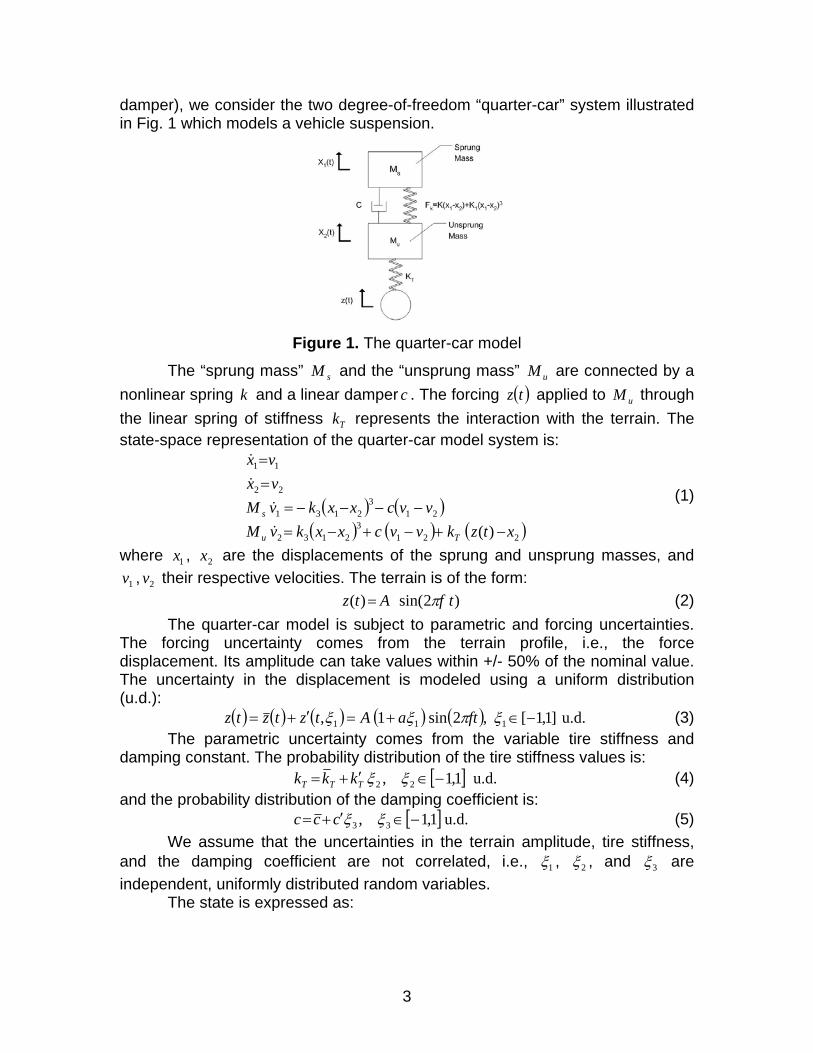
damper), we consider the two degree-of-freedom “quarter-car” system illustrated in Fig. 1 which models a vehicle suspension.

Figure 1. The quarter-car model

The “sprung mass” sM and the “unsprung mass” uM are connected by a nonlinear spring k and a linear damper c . The forcing ( )tz applied to uM through the linear spring of stiffness Tk represents the interaction with the terrain. The state-space representation of the quarter-car model system is:

( ) ( )( ) ( ) ( )221

32132

213

2131

22

11

)( xtzkvvcxxkvMvvcxxkvM

vxvx

Tu

s

−+−+−=−−−−=

==

&

&

&

&

(1)

where 1x , 2x are the displacements of the sprung and unsprung masses, and

1v , 2v their respective velocities. The terrain is of the form: )2sin()( tfAtz π= (2)

The quarter-car model is subject to parametric and forcing uncertainties. The forcing uncertainty comes from the terrain profile, i.e., the force displacement. Its amplitude can take values within +/- 50% of the nominal value. The uncertainty in the displacement is modeled using a uniform distribution (u.d.):

( ) ( ) ( ) ( ) ( ) u.d.]1,1[ ,2sin1, 111 −∈+=′+= ξπξξ ftaAtztztz (3) The parametric uncertainty comes from the variable tire stiffness and

damping constant. The probability distribution of the tire stiffness values is: [ ] u.d.1,1, 22 −∈′+= ξξTTT kkk (4)

and the probability distribution of the damping coefficient is: [ ] u.d.1,1, 33 −∈′+= ξξccc (5)

We assume that the uncertainties in the terrain amplitude, tire stiffness, and the damping coefficient are not correlated, i.e., 1ξ , 2ξ , and 3ξ are independent, uniformly distributed random variables.

The state is expressed as:

4

( ) ( ) 4,3,2,1,)(),(1

==∑=

itxtx jS

j

jii θξφθ (6)

where S is the dimension of the polynomial chaos space. Thus, the stochastic system is formulated as

( ) ( ) ( )( ) ( ) ( ) ( ) ( )jkxzkjkcvvcvM

jkcvvcvMvx

Sjvx

Tjj

Tjjj

u

jjjs

jj

jj

DBjABjA

′+−++′+−=−′−−−=

=≤≤=

23212

3211

22

11 1allfor,

&

&

&

&

(7)

where:

( ) ( ) ( )

( ) ( )( )( ) ( )

( ) ( ) ( )jkExz

jplmExxxxxx

jkEvv

S

k

kk

S

l

S

m

S

p

ppmmll

j

S

k

kk

j

,,41

,,,1

,,31

13221

1 1 142121212

13212

∑

∑∑∑

∑

=

= = =

=

−=

−−−=

−=

φ

φ

φ

jD

jB

jA

(8)

with:

( ) ( ) ( ) ( ) ( )

( ) ( ) ( ) ( ) ( )( )

( ) ( )∫ ∫ ∫

∫ ∫ ∫

∫ ∫ ∫

+

−

+

−

+

−

+

−

+

−

+

−

+

−

+

−

+

−

⋅=

⋅

⋅⋅⋅=

⋅⋅⋅=

1

1

1

1

1

1 321

2

321321

1

1

1

1

1

1 3213213213214

1

1

1

1

1

1 3213213213213213

,,

,,,,,,,,,,

,,,,,,,,,,

ξξξξφξφφ

ξξξξξξ

ξξξφξξξφξξξφξξξφ

ξξξξξξξξξφξξξφξξξφ

ddd

dddw

kjiE

dddwkjiE

kjj

lkji

kji

(9)

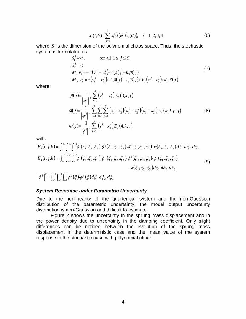
System Response under Parametric Uncertainty Due to the nonlinearity of the quarter-car system and the non-Gaussian distribution of the parametric uncertainty, the model output uncertainty distribution is non-Gaussian and difficult to estimate.

Figure 2 shows the uncertainty in the sprung mass displacement and in the power density due to uncertainty in the damping coefficient. Only slight differences can be noticed between the evolution of the sprung mass displacement in the deterministic case and the mean value of the system response in the stochastic case with polynomial chaos.

5

1 1.2 1.4 1.6 1.8 2−0.15

−0.1

−0.05

0

0.05

0.1

0.15

Time [s]

Dis

plac

emen

t [m

]

DeterministicPolyn. Chaos (mean ± 1σ)

0 1 2 3 40

30

60

90

120

150

180

Frequency [Hz]

Pow

er D

ensi

ty [m

2 s−

4 Hz−

1 ]

DeterministicPolyn. Chaos (mean ± 1 σ)

(a) Sprung mass displacement (b) Power density

Figure 2. The uncertainty in the sprung mass displacement and in the power density due to the uncertainty in the damping coefficient

Figure 3 shows the uncertainty in the sprung mass displacement and in the power density due to uncertainty in the tire stiffness. It can be seen that this type of uncertainty influences the response of the system substantially. The range of the system responses, as illustrated by the error bars in Fig. 3a, is also larger than that due to uncertainty in the damping characteristics.

1 1.2 1.4 1.6 1.8 2−0.15

−0.1

−0.05

0

0.05

0.1

0.15

Time [s]

Dis

plac

emen

t [m

]

DeterministicPolyn. Chaos (mean ± 1σ)

0 1 2 3 40

30

60

90

120

150

180

Frequency [Hz]

Pow

er D

ensi

ty [m

2 s−

4 Hz−

1 ] DeterministicPolyn. Chaos (mean ± 1 σ)

(a) Sprung mass displacement (b) Power density

Figure 3. The uncertainty in the sprung mass displacement and in the power density due to the uncertainty in the tire stiffness

Uncertainty due to Stochastic Forcing The forcing function uncertainty is first considered of the form shown in Eq. (3), where the random variable has (a) a uniform, and (b) a beta distribution, with mean 0 and support [ ]1,1− . Thus, the forcing amplitude can change between ( )aA −1 and ( )aA +1 , and has mean A . The system response is parameterized

using polynomial chaos decomposition up to order 5 (with Legendre polynomials for the uniform distribution, and Jacobi polynomials for the beta distribution). The evolution of the sprung mass position for one second of evolution is shown in Fig. 4a for the uniform forcing, and in Fig. 4b for the beta forcing. Note that the results of the deterministic simulation (using the nominal value of the amplitude) are different than the probabilistic mean due to nonlinearities, but remain within one standard deviation of it. As expected, the results for the beta uncertainty show a

6

slightly smaller variance, and a smaller difference between the stochastic mean and the deterministic solution.

0 0.2 0.4 0.6 0.8 1

−0.3

−0.2

−0.1

0

0.1

0.2

0.3

Time [s]

Dis

plac

emen

t [m

]

DeterministicPolyn. Chaos (mean ± 1σ)

0 0.2 0.4 0.6 0.8 1

−0.3

−0.2

−0.1

0

0.1

0.2

0.3

Time [s]

Dis

plac

emen

t [m

]

DeterministicPolyn. Chaos (mean ± 1σ)

(a) Amplitude uniform distributed (b) Amplitude beta distributed

Figure 4. Time evolution of sprung mass displacement for stochastic forcing with amplitude uniformly distributed and beta distributed

Uncertainty from Combined Sources In this section we present results reflecting the combined effect of both parametric uncertainty and stochastic forcing. We analyze the resulting uncertainty in both time domain and frequency domain for the quarter-car model.

Figure 5 presents the uncertainty in the sprung mass displacement, and the power density due to the combined effect of all uncertainty sources: forcing, damping parameter, and tire stiffness. The deterministic run results are different than the probabilistic mean, but they remain within one standard deviation of it.

1 1.2 1.4 1.6 1.8 2−0.15

−0.1

−0.05

0

0.05

0.1

0.15

Time [s]

Dis

plac

emen

t [m

]

DeterministicPolyn. Chaos (mean ± 1σ)

0 1 2 3 40

30

60

90

120

150

180

Frequency [Hz]

Pow

er D

ensi

ty [m

2 s−

4 Hz−

1 ]

DeterministicPolyn. Chaos (mean ± 1 σ)

(a) Sprung mass displacement (b) Power density

Figure 5. The uncertainty in the sprung mass displacement and in its power spectrum due to the combined effect of all uncertainty sources: forcing, damping

parameter, and tire stiffness Figure 6 presents the mean values (upper panels) and standard

deviations (lower panels) for the sprung mass (left panels) and unsprung mass (right panels) displacements. Shown are the moments computed from the polynomial chaos simulation, and from a Monte Carlo simulation with 2000 runs. The results are indistinguishable for the means and very close for standard

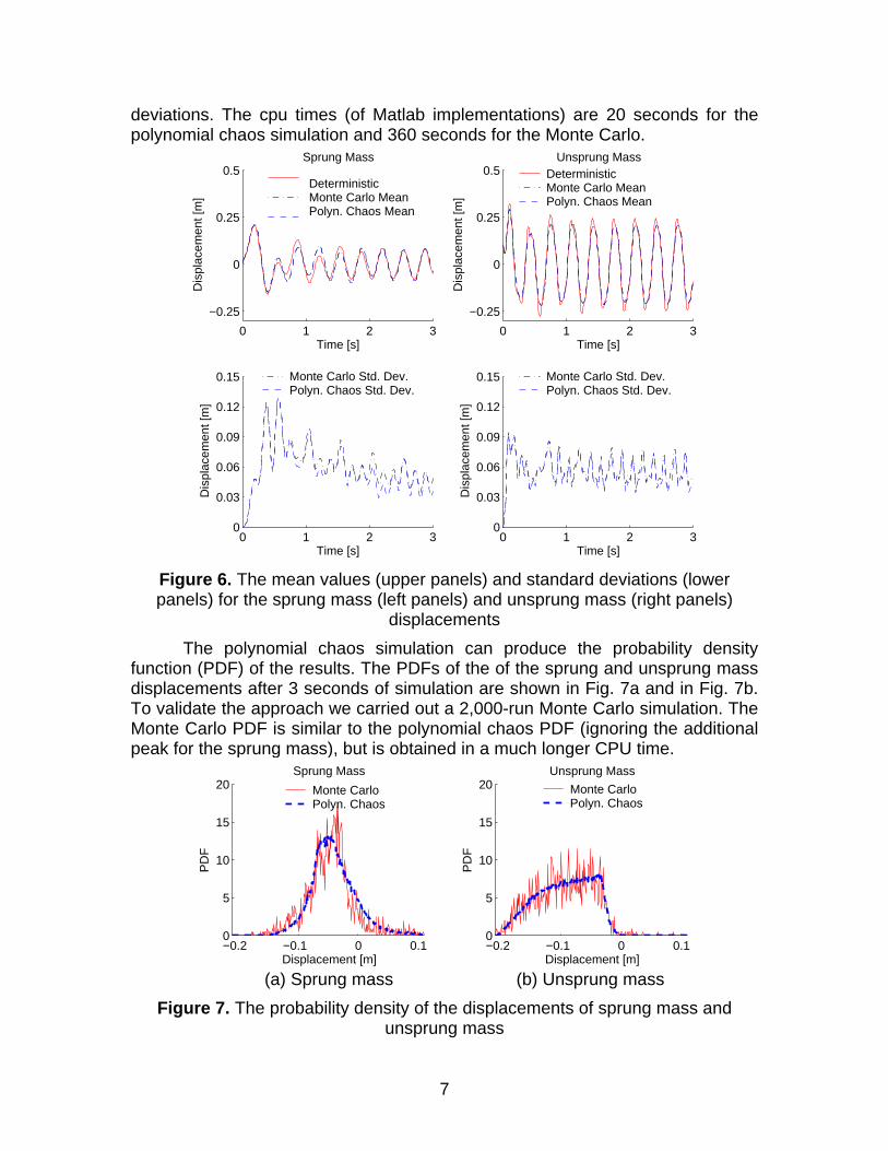
7

deviations. The cpu times (of Matlab implementations) are 20 seconds for the polynomial chaos simulation and 360 seconds for the Monte Carlo.

0 1 2 3

−0.25

0

0.25

0.5Sprung Mass

Time [s]

Dis

plac

emen

t [m

]

0 1 2 3

−0.25

0

0.25

0.5Unsprung Mass

Time [s]

Dis

plac

emen

t [m

]

0 1 2 30

0.03

0.06

0.09

0.12

0.15

Time [s]

Dis

plac

emen

t [m

]

0 1 2 30

0.03

0.06

0.09

0.12

0.15

Time [s]

Dis

plac

emen

t [m

]

Monte Carlo Std. Dev.Polyn. Chaos Std. Dev.

Monte Carlo Std. Dev.Polyn. Chaos Std. Dev.

DeterministicMonte Carlo MeanPolyn. Chaos Mean

DeterministicMonte Carlo MeanPolyn. Chaos Mean

Figure 6. The mean values (upper panels) and standard deviations (lower panels) for the sprung mass (left panels) and unsprung mass (right panels)

displacements The polynomial chaos simulation can produce the probability density

function (PDF) of the results. The PDFs of the of the sprung and unsprung mass displacements after 3 seconds of simulation are shown in Fig. 7a and in Fig. 7b. To validate the approach we carried out a 2,000-run Monte Carlo simulation. The Monte Carlo PDF is similar to the polynomial chaos PDF (ignoring the additional peak for the sprung mass), but is obtained in a much longer CPU time.

−0.2 −0.1 0 0.10

5

10

15

20Sprung Mass

Displacement [m]

PD

F

Monte CarloPolyn. Chaos

−0.2 −0.1 0 0.10

5

10

15

20

Displacement [m]

PD

F

Unsprung Mass

Monte CarloPolyn. Chaos

(a) Sprung mass (b) Unsprung mass

Figure 7. The probability density of the displacements of sprung mass and unsprung mass

8

2670

1780

890

0

890

1780

2670

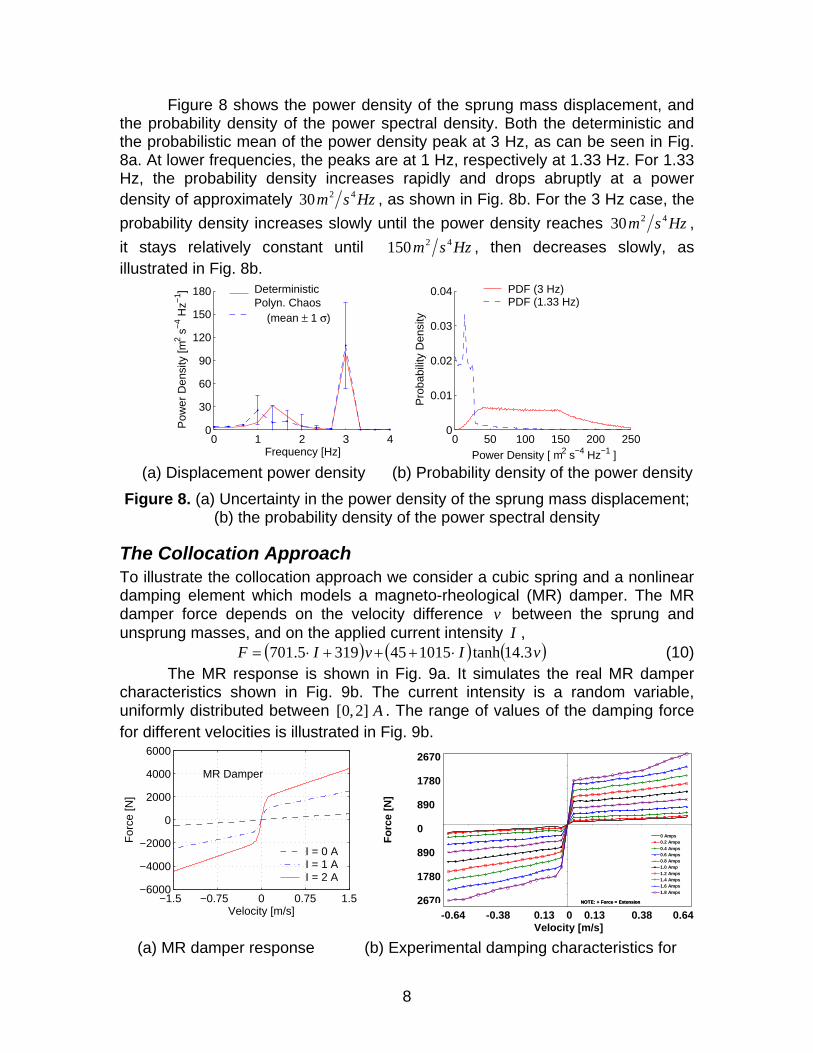
Figure 8 shows the power density of the sprung mass displacement, and the probability density of the power spectral density. Both the deterministic and the probabilistic mean of the power density peak at 3 Hz, as can be seen in Fig. 8a. At lower frequencies, the peaks are at 1 Hz, respectively at 1.33 Hz. For 1.33 Hz, the probability density increases rapidly and drops abruptly at a power density of approximately Hzsm 4230 , as shown in Fig. 8b. For the 3 Hz case, the probability density increases slowly until the power density reaches Hzsm 4230 , it stays relatively constant until Hzsm 42150 , then decreases slowly, as illustrated in Fig. 8b.

0 1 2 3 40

30

60

90

120

150

180

Frequency [Hz]

Pow

er D

ensi

ty [m

2 s−

4 Hz−

1 ] DeterministicPolyn. Chaos (mean ± 1 σ)

0 50 100 150 200 2500

0.01

0.02

0.03

0.04

Power Density [ m2 s−4 Hz−1 ]

Pro

babi

lity

Den

sity

PDF (3 Hz)PDF (1.33 Hz)

(a) Displacement power density (b) Probability density of the power density Figure 8. (a) Uncertainty in the power density of the sprung mass displacement;

(b) the probability density of the power spectral density

The Collocation Approach To illustrate the collocation approach we consider a cubic spring and a nonlinear damping element which models a magneto-rheological (MR) damper. The MR damper force depends on the velocity difference v between the sprung and unsprung masses, and on the applied current intensity I ,

( ) ( ) ( )vIvIF 3.14tanh1015453195.701 ⋅+++⋅= (10) The MR response is shown in Fig. 9a. It simulates the real MR damper

characteristics shown in Fig. 9b. The current intensity is a random variable, uniformly distributed between A]2,0[ . The range of values of the damping force for different velocities is illustrated in Fig. 9b.

−1.5 −0.75 0 0.75 1.5−6000

−4000

−2000

0

2000

4000

6000

Velocity [m/s]

For

ce [N

]

MR Damper

I = 0 AI = 1 AI = 2 A

(a) MR damper response (b) Experimental damping characteristics for

Forc

e [N

]

-0.64 -0.38 0.13 0 0.13 0.38 0.64 Velocity [m/s]

0 Amps0.2 Amps0.4 Amps0.6 Amps0.8 Amps1.0 Amp1.2 Amps1.4 Amps1.6 Amps1.8 Amps

NOTE: + Force = Extension

Note: Curves have been zeroedas described in the text.

0 Amps0.2 Amps0.4 Amps0.6 Amps0.8 Amps1.0 Amp1.2 Amps1.4 Amps1.6 Amps1.8 Amps

NOTE: + Force = Extension

Note: Curves have been zeroedas described in the text.

9

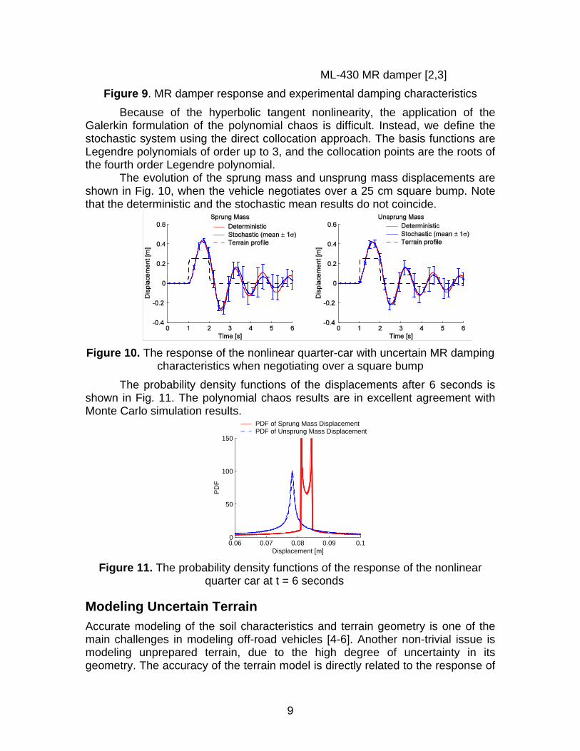
ML-430 MR damper [2,3] Figure 9. MR damper response and experimental damping characteristics

Because of the hyperbolic tangent nonlinearity, the application of the Galerkin formulation of the polynomial chaos is difficult. Instead, we define the stochastic system using the direct collocation approach. The basis functions are Legendre polynomials of order up to 3, and the collocation points are the roots of the fourth order Legendre polynomial.

The evolution of the sprung mass and unsprung mass displacements are shown in Fig. 10, when the vehicle negotiates over a 25 cm square bump. Note that the deterministic and the stochastic mean results do not coincide.

Figure 10. The response of the nonlinear quarter-car with uncertain MR damping

characteristics when negotiating over a square bump The probability density functions of the displacements after 6 seconds is

shown in Fig. 11. The polynomial chaos results are in excellent agreement with Monte Carlo simulation results.

0.06 0.07 0.08 0.09 0.10

50

100

150

Displacement [m]

PD

F

PDF of Sprung Mass DisplacementPDF of Unsprung Mass Displacement

Figure 11. The probability density functions of the response of the nonlinear

quarter car at t = 6 seconds

Modeling Uncertain Terrain Accurate modeling of the soil characteristics and terrain geometry is one of the main challenges in modeling off-road vehicles [4-6]. Another non-trivial issue is modeling unprepared terrain, due to the high degree of uncertainty in its geometry. The accuracy of the terrain model is directly related to the response of

10

the vehicle analyzed, such as its mobility. It is clear that a deterministic approach is not suitable in this case [7], and the uncertainties in the terrain profile must be taken into account.

The proposed terrain model exemplifies the use of Karhunen-Loeve (KL) expansion to represent stochastic forcings. KL expansion is based on the eigenfunctions and eigenvalues of the covariance function. As explained in the companion paper [1], the covariance function of the forcing can be determined experimentally, for example from power spectrum density data.

We consider a one-dimensional course with an uncertain profile. The terrain height is periodic in space with a period D and is modeled as a stochastic process periodic in space.

( ) ( )

( )

integersand,2

,2

2sin

sincossincos

212

21

1

0

222

2212

112

1111

nnn

DLn

DL

DxAxz

Lx

LxA

Lx

LxAxzxz

ππ

π

ξξξξ

==

⎟⎠⎞

⎜⎝⎛=

⎟⎟⎠

⎞⎜⎜⎝

⎛⎟⎟⎠

⎞⎜⎜⎝

⎛+⎟⎟

⎠

⎞⎜⎜⎝

⎛+⎟⎟

⎠

⎞⎜⎜⎝

⎛⎟⎟⎠

⎞⎜⎜⎝

⎛+⎟⎟

⎠

⎞⎜⎜⎝

⎛+=

(11)

In Eq. (11) ijξ are independent normal random variables of mean 0 and standard deviation 1. The terrain height at each location x is a normal random variable of mean )(xz and standard deviation 2

22

1 AA + . The correlation between terrain heights at two spatial points is

( ) ( ) ( )[ ] ⎟⎟⎠

⎞⎜⎜⎝

⎛ −+⎟⎟

⎠

⎞⎜⎜⎝

⎛ −=−−=

2

2122

1

2121221121 coscos)()()()(,

LxxA

LxxAxzxzxzxzExxR (12)

We regard the stochastic process from Eq. (11) as the superposition of two periodic stochastic processes with correlation lengths 1L and 2L respectively. The correlation function )( 21 xxR − is also periodic with period D . Lucor et. al. [8] show that the Karhunen-Loeve representation of a periodic stochastic process is:

( ) ∑∞

=⎥⎦

⎤⎢⎣

⎡⎟⎠⎞

⎜⎝⎛+⎟

⎠⎞

⎜⎝⎛+=

10

0 2sin2cos2,n

sncnnc Dxn

Dxn

DDxz πξπξλξλξ (13)

They also establish that the eigenvectors of the periodic covariance kernel are )/cos( nLx , )/sin( nLx , where the correlation length of the thn eigenvector is

)2/( nDLn π= . The periodic correlation function in Eq. (12) has only two nonzero eigenvalues,

222

211 2

,2

ADAD== λλ (14)

From Eq. (13) and Eq. (14) we conclude that Eq. (11) is the Karhunen-Loeve representation of the periodic stochastic process with covariance given by Eq. (12). The choice of the model Eq. (11) is motivated by the analysis of Lucor et al. [8]. The authors consider bilateral autoregressive processes of the form:

11

( ) ( ) ( )i

iii axxzxxzbxz ξ+

∆−+∆+=

2 (15)

Intuitively, the terrain height at ix depends on the average of terrain heights at locations situated both to its left and to its right, plus a random term. In [8] it is shown that, in the continuous limit 0→∆x , 1→b , and for particular choices of the correlation lengths, the second order autoregressive process from Eq. (15) can be represented as in Eq. (11).

In the numerical experiments presented next we consider the following numerical values:

mDLmDLmAmAmAmD 3.214

,3.56

,1.0,2.0,5.0,100 21210 ≅=≅=====ππ

(16)

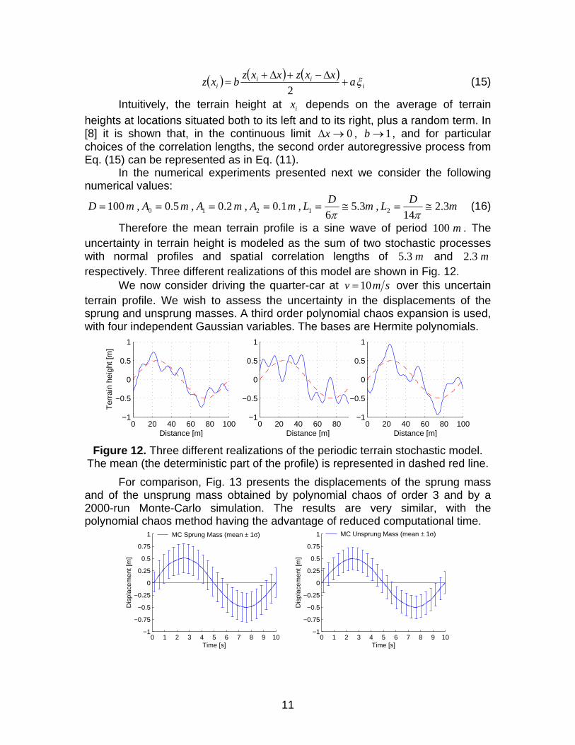
Therefore the mean terrain profile is a sine wave of period m100 . The uncertainty in terrain height is modeled as the sum of two stochastic processes with normal profiles and spatial correlation lengths of m3.5 and m3.2 respectively. Three different realizations of this model are shown in Fig. 12.

We now consider driving the quarter-car at smv 10= over this uncertain terrain profile. We wish to assess the uncertainty in the displacements of the sprung and unsprung masses. A third order polynomial chaos expansion is used, with four independent Gaussian variables. The bases are Hermite polynomials.

0 20 40 60 80 100−1

−0.5

0

0.5

1

Ter

rain

hei

ght [

m]

Distance [m]0 20 40 60 80 1

−1

−0.5

0

0.5

1

Distance [m]0 20 40 60 80 100

−1

−0.5

0

0.5

1

Distance [m] Figure 12. Three different realizations of the periodic terrain stochastic model.

The mean (the deterministic part of the profile) is represented in dashed red line. For comparison, Fig. 13 presents the displacements of the sprung mass

and of the unsprung mass obtained by polynomial chaos of order 3 and by a 2000-run Monte-Carlo simulation. The results are very similar, with the polynomial chaos method having the advantage of reduced computational time.

0 1 2 3 4 5 6 7 8 9 10−1

−0.75

−0.5

−0.25

0

0.25

0.5

0.75

1

Time [s]

Dis

plac

emen

t [m

]

MC Sprung Mass (mean ± 1σ)

0 1 2 3 4 5 6 7 8 9 10−1

−0.75

−0.5

−0.25

0

0.25

0.5

0.75

1

Time [s]

Dis

plac

emen

t [m

]

MC Unsprung Mass (mean ± 1σ)

12

Figure 13. Time evolution of the displacements of sprung and unsprung masses

obtained by polynomial chaos of order 3 and by a 2000-run Monte-Carlo. Figure 14 illustrates the probability density functions at the final time for

the sprung and unsprung masses. The polynomial chaos and the 2000-run Monte-Carlo estimates give similar results.

−1 −0.5 0 0.5 10

0.5

1

1.5

2

Sprung Mass Displacement [m]

PD

F

Polyn. ChaosMonte Carlo

−1 −0.5 0 0.5 10

0.5

1

1.5

2

Unsprung Mass Displacement [m]

PD

F

Polyn. ChaosMonte Carlo

Figure 14. The probability density function at the final time for the sprung and unsprung masses.

Polynomial Chaos versus Statistical Linearization Statistical linearization is a powerful approach to approximate the mean and variance of the response of nonlinear dynamic systems to stochastic perturbations [9]. To compare polynomial chaos with statistical linearization, consider the single degree of freedom nonlinear oscillator:

( ) )(tfxgxcxm =++ &&& (17) where )(tf is a stochastic forcing and )(xg a nonlinear spring. The system in Eq. (17) is approximated by a linear system [9]:

)(tfkyycym =++ &&& (18) with the “equivalent stiffness” coefficient k chosen such that the mean-square response ][ 2yE of the linear system is an optimal estimate of the mean square response ][ 2xE of the nonlinear system in Eq. (17). Based on this approximation, and assuming the response of the system in Eq. (18) has zero mean, its variance is given by:

13

[ ] ( )( )∫

∞

∞− +−= ω

ωω

ωd

cmk

SyE f

22222 (19)

where )(ωfS is the spectral density of the stochastic excitation )(tf . The standard equivalent linearization applied to the one-dimensional

system in Eq. (17) provides the following formula for the equivalent stiffness coefficient [9]:

( )[ ][ ]22 ][

)]([yE

yygExE

xgxEk ≈= (20)

The value of this coefficient can be derived only if the statistics of the nonlinear solution x are known. In practice these statistics are approximated by the statistics of the linear response y , which is often assumed Gaussian. Equations (19) and (20) are solved simultaneously for k and ][ 2yE .

We consider a nonlinear cubic spring with 3)( xhxg = . Under the Gaussian assumption for the distribution of y we have that

( ) ][3][][3

][][ 2

2

22

2

4

yEhyEyEh

yEyhEk ==≈ (21)

Consider the stochastic forcing be the stochastic terrain surface in Eq. (11) with zero mean, ( ) 0=xz . The power density of this forcing is:

( ) ( ) ( ))()(2

)()(2

12

12

22

11

11

21

−−−− ++−+++−= LLALLAS f ωδωδπωδωδπω (22)

From Eq. (19) and Eq. (22) the variance of the response is obtained:

[ ] ( ) ( ) 22

2222

22

21

2221

212 22

−−−− +−+

+−=

LcmLkA

LcmLkA

yEππ

(23)

Equations (21) and (23) are solved together for k and ][ 2yE . In the numerical experiments presented below we use the following

numerical values (in non-dimensional units): [ ]200,0,2,4,1,1,10 21 ∈===== tAAhcm (24)

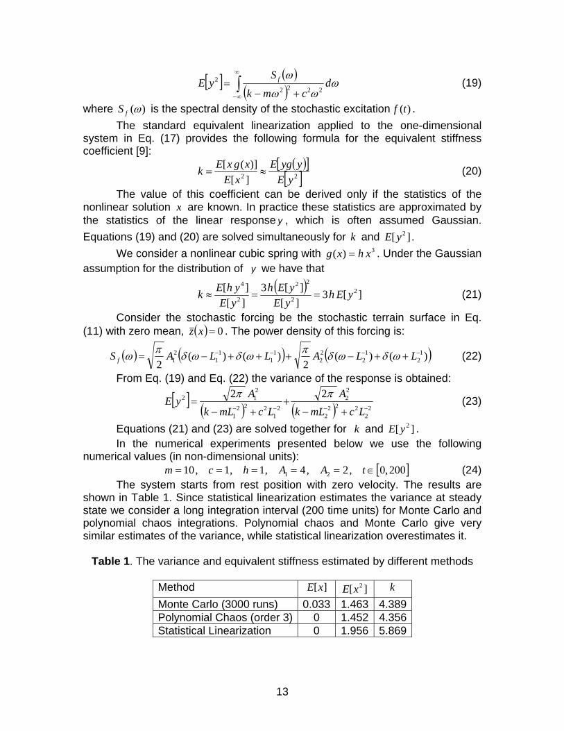
The system starts from rest position with zero velocity. The results are shown in Table 1. Since statistical linearization estimates the variance at steady state we consider a long integration interval (200 time units) for Monte Carlo and polynomial chaos integrations. Polynomial chaos and Monte Carlo give very similar estimates of the variance, while statistical linearization overestimates it.

Table 1. The variance and equivalent stiffness estimated by different methods

Method ][xE ][ 2xE k Monte Carlo (3000 runs) 0.033 1.463 4.389 Polynomial Chaos (order 3) 0 1.452 4.356 Statistical Linearization 0 1.956 5.869

14

We conclude this comparison by noting that the shorter the correlation time/distance of the stochastic forcing is, the more terms are needed in the Karhunen-Loeve expansion for a given accuracy. The polynomial chaos approach becomes impractical for weakly correlated forcings (and in particular for white noise forcing).

Special Dynamical Behavior We study the quality of the polynomial chaos approximation for two systems with very particular dynamics. The first example is the double-well problem; the PDF of the solution becomes bi-modal and difficult to approximate by smooth polynomials. The second example is the chaotic 3-variable Lorenz model; with proper initial values, the solutions collapse onto an attractive manifold. We expect the chaotic dynamics to challenge the polynomial chaos approximations of the PDF.

The Double-Well Problem The double-well problem is governed by the ordinary differential equations (ODEs):

( ) ( ) 02 0,20,1 xxtxxx =≤≤−−=& (25)

There are two stable attractors at 1±=x , and one unstable steady state at 0=x . For every negative initial condition 00 <x the system evolves toward the

attractive steady state 1−=x , and for every 00 >x toward 1+=x . Thus any probability distribution of the initial state (which spans both positive and negative values) will evolve toward a couple of Dirac distributions on the attractor states. The problem is challenging since the state probability density becomes less smooth as the system evolves, making it increasingly difficult to construct spectral approximations.

Consider the case where the initial state is uniformly distributed between ]375.0,625.0[− , as shown in Fig. 15a. Since this distribution is skewed to the left,

we expect the system to reach the final state 1−=x with higher probability than 1+=x . The resulting PDF was computed with Monte Carlo (10,000 runs) and

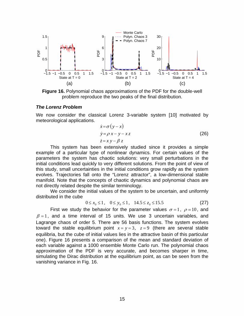
Legendre chaos of orders 3 and 7. The results are shown in Fig. 15b for 2=t and in Fig. 15c for 4=t . We notice that the polynomial chaos approximation captures the bimodal result distribution. For 2=t the PDF calculated by polynomial chaos is reasonably accurate. As the real distribution approaches two Dirac functions, the quality of the polynomial chaos PDF decreases, as seen in Fig. 15c. Nevertheless, the bimodal character is well captured, with the probability of the left final state being larger than that of the right final state.

15

−1.5 −1 −0.5 0 0.5 1 1.50

0.5

1

1.5

State at T = 0

PD

F

−1.5 −1 −0.5 0 0.5 1 1.50

3

6

9

State at T = 2

PD

F

−1.5 −1 −0.5 0 0.5 1 1.50

10

20

30

State at T = 4

PD

F

Monte CarloPolyn. Chaos 3Polyn. Chaos 7

(a) (b) (c)

Figure 16. Polynomial chaos approximations of the PDF for the double-well problem reproduce the two peaks of the final distribution.

The Lorenz Problem We now consider the classical Lorenz 3-variable system [10] motivated by meteorological applications.

( )

zyxzzxyxy

xyx

βρσ

−=−−=

−=

&

&

&

(26)

This system has been extensively studied since it provides a simple example of a particular type of nonlinear dynamics. For certain values of the parameters the system has chaotic solutions: very small perturbations in the initial conditions lead quickly to very different solutions. From the point of view of this study, small uncertainties in the initial conditions grow rapidly as the system evolves. Trajectories fall onto the “Lorenz attractor”, a low-dimensional stable manifold. Note that the concepts of chaotic dynamics and polynomial chaos are not directly related despite the similar terminology.

We consider the initial values of the system to be uncertain, and uniformly distributed in the cube

5.155.14,10,10 000 ≤≤≤≤≤≤ zyx (27) First we study the behavior for the parameter values 1=σ , 10=ρ , and

1=β , and a time interval of 15 units. We use 3 uncertain variables, and Lagrange chaos of order 5. There are 56 basis functions. The system evolves toward the stable equilibrium point ,3== yx 9=z (there are several stable equilibria, but the cube of initial values lies in the attractive basin of this particular one). Figure 16 presents a comparison of the mean and standard deviation of each variable against a 1000 ensemble Monte Carlo run. The polynomial chaos approximation of the PDF is very accurate, and becomes sharper in time, simulating the Dirac distribution at the equilibrium point, as can be seen from the vanishing variance in Fig. 16.

16

0 5 10 150

1

2

3

4X mean

0 5 10 15−1

0

1

2

3

4

5

6Y mean

0 5 10 152

4

6

8

10

12

14

16Z mean

0 5 10 150

0.2

0.4

0.6

0.8

1

1.2

1.4X std

Time units0 5 10 15

0

0.5

1

1.5

2

2.5Y std

Time units0 5 10 15

0

1

2

3

4Z std

Time units

Monte CarloPolyn. Chaos

Figure 16. Lorenz system, the stable attractor case. The polynomial chaos

approximation of the PDF is very accurate. Next, we consider the parameter values that were originally chosen by

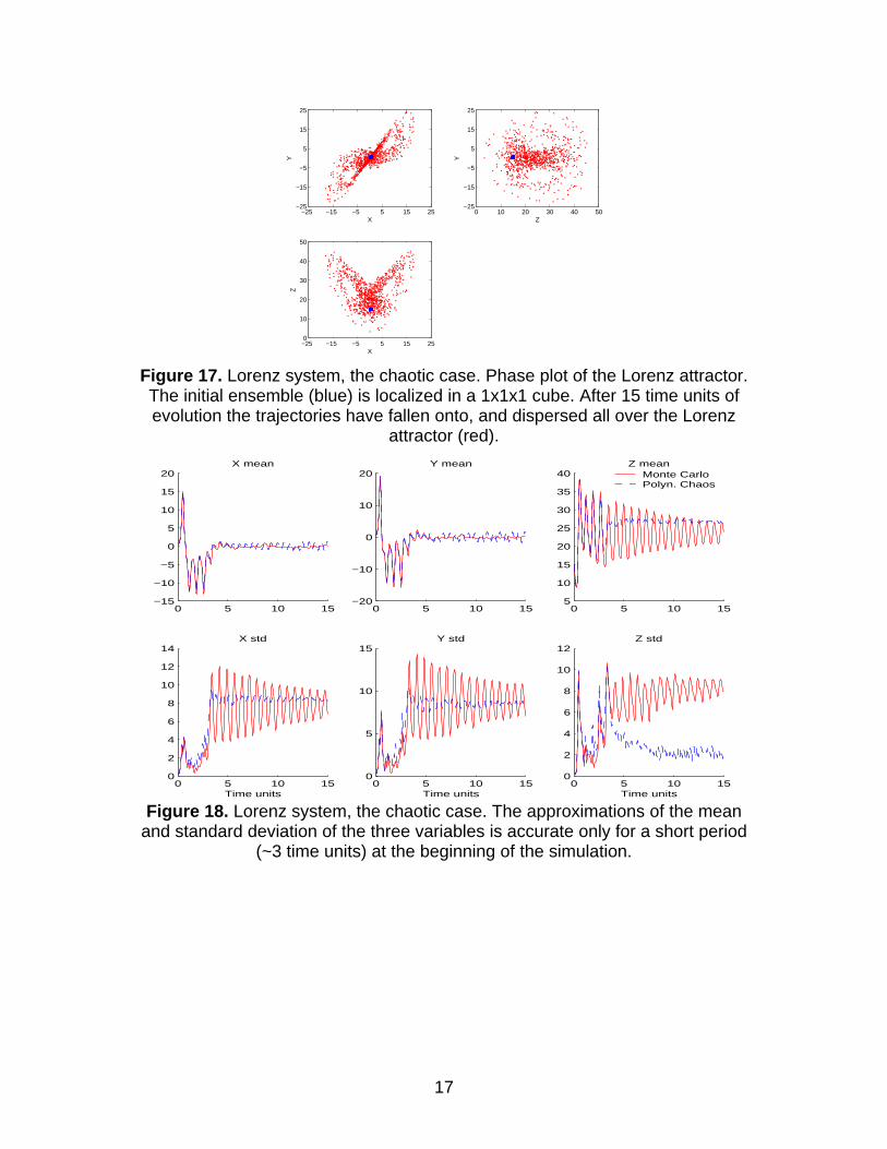
Lorenz [10] to obtain chaotic dynamics: 10=σ , 28=ρ , and 38=β . A phase plot of the Lorenz attractor can be seen in Fig. 17. The attractor has a complicated geometry, which makes it difficult for polynomial chaos to approximate it.

The cube of initial values lies near the attractor, as seen in Fig. 17 (blue dots). Even if the set of initial conditions is very localized, after 15 time units the trajectories have diverged and span all the attractor, as seen in Fig. 17 (red dots). This behavior is typical for chaotic dynamics, and is what makes this test case challenging for polynomial chaos approximations.

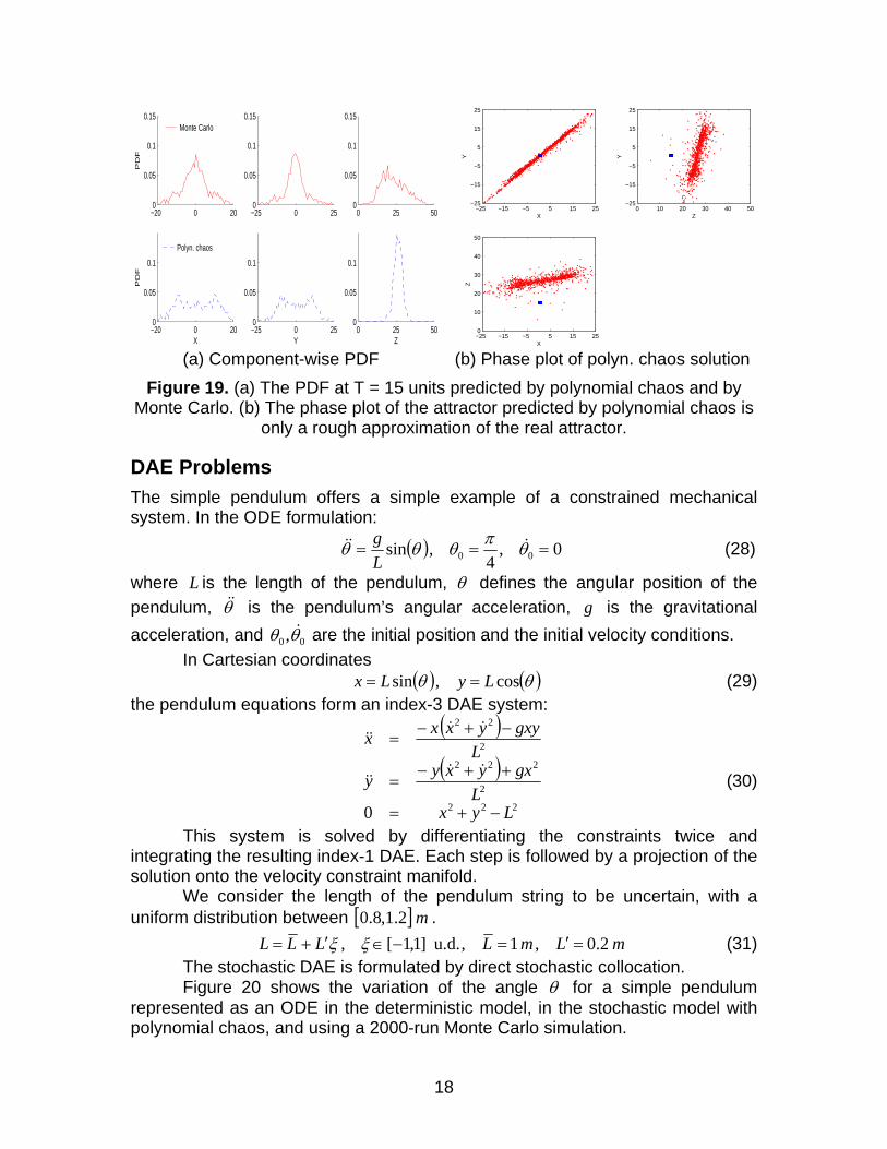
Figure 18 compares the mean and standard deviations obtained by polynomial chaos with a 1000 ensemble Monte Carlo run. The rapid increase in standard deviation in the beginning reflects the rapid amplification of uncertainty, in chaotic dynamics. We notice that polynomial chaos approximation is quite accurate in the very beginning (for about 3 time units). After that the approximation of the Z mean, as well as the standard deviations, become inaccurate. The polynomial chaos PDF after 15 time units is shown in Fig. 19a. It is not a very accurate approximation of the PDF estimated by Monte Carlo. The phase plot of the polynomial chaos predicted distribution is shown in Fig. 19b. This phase plot reveals that an attractor is also predicted by the polynomial chaos approach. Its shape, however, is only a rough approximation of the real attractor shown in Fig. 17.

17

−25 −15 −5 5 15 25−25

−15

−5

5

15

25

X

Y

0 10 20 30 40 50−25

−15

−5

5

15

25

Z

Y

−25 −15 −5 5 15 250

10

20

30

40

50

X

Z

Figure 17. Lorenz system, the chaotic case. Phase plot of the Lorenz attractor. The initial ensemble (blue) is localized in a 1x1x1 cube. After 15 time units of evolution the trajectories have fallen onto, and dispersed all over the Lorenz

attractor (red).

0 5 10 15−15

−10

−5

0

5

10

15

20X mean

0 5 10 15−20

−10

0

10

20Y mean

0 5 10 155

10

15

20

25

30

35

40Z mean

Monte CarloPolyn. Chaos

0 5 10 150

2

4

6

8

10

12

14X std

Time units0 5 10 15

0

5

10

15Y std

Time units0 5 10 15

0

2

4

6

8

10

12Z std

Time units Figure 18. Lorenz system, the chaotic case. The approximations of the mean

and standard deviation of the three variables is accurate only for a short period (~3 time units) at the beginning of the simulation.

18

−20 0 200

0.05

0.1

0.15

PD

FMonte Carlo

−25 0 250

0.05

0.1

0.15

0 25 500

0.05

0.1

0.15

−20 0 200

0.05

0.1

X

PD

F

Polyn. chaos

−25 0 250

0.05

0.1

Y0 25 50

0

0.05

0.1

Z

−25 −15 −5 5 15 25−25

−15

−5

5

15

25

X

Y

0 10 20 30 40 50−25

−15

−5

5

15

25

Z

Y

−25 −15 −5 5 15 250

10

20

30

40

50

X

Z

(a) Component-wise PDF (b) Phase plot of polyn. chaos solution

Figure 19. (a) The PDF at T = 15 units predicted by polynomial chaos and by Monte Carlo. (b) The phase plot of the attractor predicted by polynomial chaos is

only a rough approximation of the real attractor.

DAE Problems The simple pendulum offers a simple example of a constrained mechanical system. In the ODE formulation:

( ) 0,4

,sin 00 === θπθθθ &&&Lg (28)

where L is the length of the pendulum, θ defines the angular position of the pendulum, θ&& is the pendulum’s angular acceleration, g is the gravitational acceleration, and 00 ,θθ & are the initial position and the initial velocity conditions.

In Cartesian coordinates ( ) ( )θθ cos,sin LyLx == (29)

the pendulum equations form an index-3 DAE system:

( )( )

222

2

222

2

22

0 LyxL

gxyxyy

Lgxyyxxx

−+=

++−=

−+−=

&&&&

&&&&

(30)

This system is solved by differentiating the constraints twice and integrating the resulting index-1 DAE. Each step is followed by a projection of the solution onto the velocity constraint manifold.

We consider the length of the pendulum string to be uncertain, with a uniform distribution between [ ]m2.1,8.0 .

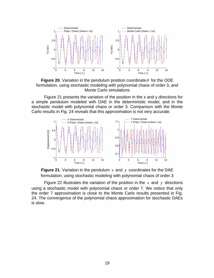
mLmLLLL 2.0,1,u.d.]1,1[, =′=−∈′+= ξξ (31) The stochastic DAE is formulated by direct stochastic collocation. Figure 20 shows the variation of the angle θ for a simple pendulum

represented as an ODE in the deterministic model, in the stochastic model with polynomial chaos, and using a 2000-run Monte Carlo simulation.

19

0 3 6 9 12 15−1

−0.5

0

0.5

1

θ [ r

ad ]

Time [ s ]

DeterministicPolyn. Chaos (mean ± 1σ)

0 3 6 9 12 15−1

−0.5

0

0.5

1

θ [ r

ad ]

Time [ s ]

DeterministicMonte Carlo (mean ± 1σ)

Figure 20. Variation in the pendulum position coordinateθ for the ODE

formulation, using stochastic modeling with polynomial chaos of order 3, and Monte Carlo simulations

Figure 21 presents the variation of the position in the x and y directions for a simple pendulum modeled with DAE in the deterministic model, and in the stochastic model with polynomial chaos or order 3. Comparison with the Monte Carlo results in Fig. 24 reveals that this approximation is not very accurate.

0 3 6 9 12 15−1

−0.5

0

0.5

1

Time [ s ]

Dis

plac

emen

t [m

]

X DeterministicX Polyn. Chaos (mean ± 1σ)

0 3 6 9 12 15

0.7

0.8

0.9

1

1.1

Time [ s ]

Y DeterministicY Polyn. Chaos (mean ± 1σ)

Figure 21. Variation in the pendulum x and y coordinates for the DAE formulation, using stochastic modeling with polynomial chaos of order 3

Figure 22 illustrates the variation of the position in the x and y directions using a stochastic model with polynomial chaos or order 7. We notice that only the order 7 approximation is close to the Monte Carlo results presented in Fig. 24. The convergence of the polynomial chaos approximation for stochastic DAEs is slow.

20

0 3 6 9 12 15−1

−0.5

0

0.5

1

Time [ s ]

Dis

plac

emen

t [m

]

X DeterministicX Polyn. Chaos (mean ± 1σ)

0 3 6 9 12 15

0.7

0.8

0.9

1

1.1

Time [ s ]

Y DeterministicY Polyn. Chaos (mean ± 1σ)

Figure 22. Variation in the pendulum x and y coordinates for the DAE formulation, using stochastic modeling with polynomial chaos of order 7

Figure 23 shows the variation of the position in the x and y directions for a simple pendulum modeled with DAE in the deterministic model, and in the 2000-run Monte Carlo simulation.

0 3 6 9 12 15−1

−0.5

0

0.5

1

Dis

plac

emen

t [m

]

Time [ s ]

X DeterministicX Monte Carlo

0 3 6 9 12 15

0.7

0.8

0.9

1

1.1

Time [ s ]

Y DeterministicY Monte Carlo

Figure 23. Variation in the pendulum x and y coordinates for the DAE

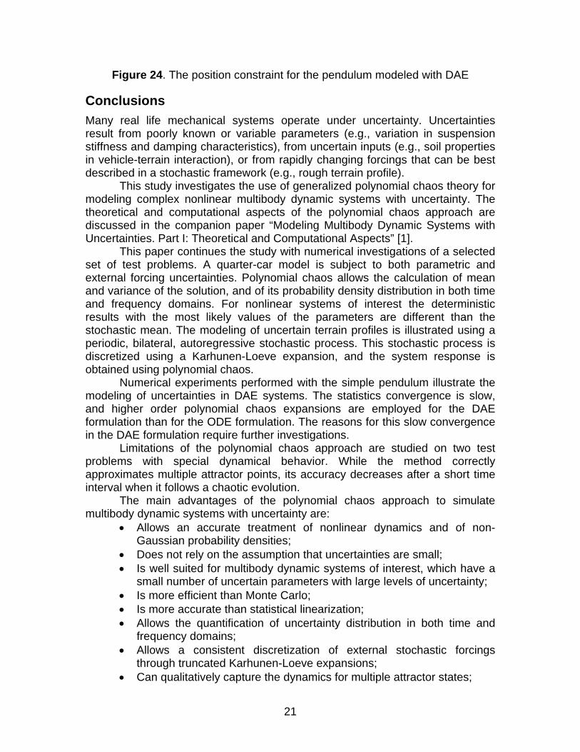
formulation, using a 2000-run Monte Carlo simulation Figure 24a presents the position constraint for a simple pendulum

modeled with the stochastic model with polynomial chaos of order 3, and Fig. 24b for polynomial chaos of order 7. The order 3 approximation shows an increase in variance after about 10 seconds, which confirms that the convergence of the polynomial chaos approach for DAE problems is slow.

0 3 6 9 12 150

0.5

1

1.5

Time [ s ]

PositionConstraint (X2+Y2)

0 3 6 9 12 150

0.2

0.4

0.6

0.8

1

1.2

1.4

Time [ s ]

PositionConstraint (X2+Y2)

(a) Polynomial chaos of order 3 (b) Polynomial chaos of order 7

21

Figure 24. The position constraint for the pendulum modeled with DAE

Conclusions Many real life mechanical systems operate under uncertainty. Uncertainties result from poorly known or variable parameters (e.g., variation in suspension stiffness and damping characteristics), from uncertain inputs (e.g., soil properties in vehicle-terrain interaction), or from rapidly changing forcings that can be best described in a stochastic framework (e.g., rough terrain profile).

This study investigates the use of generalized polynomial chaos theory for modeling complex nonlinear multibody dynamic systems with uncertainty. The theoretical and computational aspects of the polynomial chaos approach are discussed in the companion paper “Modeling Multibody Dynamic Systems with Uncertainties. Part I: Theoretical and Computational Aspects” [1].

This paper continues the study with numerical investigations of a selected set of test problems. A quarter-car model is subject to both parametric and external forcing uncertainties. Polynomial chaos allows the calculation of mean and variance of the solution, and of its probability density distribution in both time and frequency domains. For nonlinear systems of interest the deterministic results with the most likely values of the parameters are different than the stochastic mean. The modeling of uncertain terrain profiles is illustrated using a periodic, bilateral, autoregressive stochastic process. This stochastic process is discretized using a Karhunen-Loeve expansion, and the system response is obtained using polynomial chaos.

Numerical experiments performed with the simple pendulum illustrate the modeling of uncertainties in DAE systems. The statistics convergence is slow, and higher order polynomial chaos expansions are employed for the DAE formulation than for the ODE formulation. The reasons for this slow convergence in the DAE formulation require further investigations.

Limitations of the polynomial chaos approach are studied on two test problems with special dynamical behavior. While the method correctly approximates multiple attractor points, its accuracy decreases after a short time interval when it follows a chaotic evolution.

The main advantages of the polynomial chaos approach to simulate multibody dynamic systems with uncertainty are:

• Allows an accurate treatment of nonlinear dynamics and of non-Gaussian probability densities;

• Does not rely on the assumption that uncertainties are small; • Is well suited for multibody dynamic systems of interest, which have a

small number of uncertain parameters with large levels of uncertainty; • Is more efficient than Monte Carlo; • Is more accurate than statistical linearization; • Allows the quantification of uncertainty distribution in both time and

frequency domains; • Allows a consistent discretization of external stochastic forcings

through truncated Karhunen-Loeve expansions; • Can qualitatively capture the dynamics for multiple attractor states;

22

• Allows simulations for uncertain differential-algebraic equations. The main weaknesses of the polynomial chaos approach are: • The dimension of the stochastic space increases exponentially with the

number of independent random variables. Consequently, the approach is efficient only for a relatively small number of sources of uncertainty;

• The discretization of external stochastic forcings by truncated Karhunen-Loeve expansions require many terms for processes with short correlation lengths/times;

• Treatment of non-polynomial nonlinearities in the Galerkin framework requires the use of multidimensional quadrature rules. On the other hand, a complete convergence theory for the less expensive collocation approach is not available at this time;

• For chaotic dynamics the approximation of the PDF is accurate only for short simulation times;

• The convergence of the method for the DAE (pendulum) example is notably slower than for the ODE formulation of the same system.

The overall conclusion is that despite its limitations, polynomial chaos is a powerful and potentially very useful, approach for the simulation of multibody dynamic systems with uncertainty.

Acknowledgements The work of A. Sandu was supported in part by NSF through the awards CAREER ACI-0093139 and ITR AP&IM 0205198. The work of C. Sandu was supported in part by the AdvanceVT faculty development grant 477201 from Virginia Tech’s NSF ADVANCE Award 0244916.

References [1] Sandu, A., Sandu, C., and Ahmadian, M., “Modeling Multibody Dynamic Systems with Uncertainties. Part I: Theoretical Development”, submitted Sept. 2004.

[2] Ahmadian, M., Appleton, R., and Norris, J. A., “Designing Magneto-Rheological Recoil Dampers in a Fire-out-of Battery Recoil System”, IEEE Transactions on Magnetics, Vol. 37, No. 1, Jan. 2003, pp. 430 – 435.

[3] Ahmadian, M. and Poynor, J.C., “Effective Test Procedure for Evaluating Force Characteristics of Magneto-rheological Dampers”, Proc. of ASME IMECE 2003, IMECE2003-38153, Nov. 15 – 21, 2003, Washington, D.C.

[4] Bekker, M.G., Theory of Land Locomotion, The U. of Michigan Press, Ann Arbor, Michigan, 1956.

[5] Bekker, M.G., Off-the-Road Locomotion, The University of Michigan Press, Ann Arbor, 1960.

[6] Bekker, M.G., Introduction to Terrain-Vehicle Systems, The University of Michigan Press, Ann Arbor, Michigan, 1969.

23

[7] Harnisch, C., and Jakobs, R., “Impact of Scattering Soil Strength and Roughness on Terrain Vehicle Dynamics”, Proc. of the 13th Int. Conf. of ISTVS, Munich, Germany, 1999.

[8] Lucor, D., Su, C.-H., and Karniadakis, G.E., Karhunen-Loeve Representation of Periodic Second Order Autoregressive Processes, M. Bubak editor, ICCS 2004, LNCS 3038, pp. 827-834, Springer-Verlag, 2004.

[9] Crandall, S.H., “Is Stochastic Linearization a fundamentally flawed procedure?”, Probabilistic Engineering Mechanics, Vol. 16, pp. 169-176, 2001.

[10] Lorenz, E.M., “Deterministic Nonperiodic Flow”, J. Atmos. Sci., 20, 448-464, 1963.