Model-Based Machine Learning for

Fiber-Optic Communication Systems

Christian Häger(1)

Joint work with: Henry D. Pfister(2), Rick M. Bütler(3),

Gabriele Liga(3), Alex Alvarado(3), Christoffer Fougstedt(4),

Lars Svensson(4), and Per Larsson-Edefors(4)

(1)Department of Electrical Engineering, Chalmers University of Technology, Sweden(2)Department of Electrical and Computer Engineering, Duke University, USA

(3)Department of Electrical Engineering, Eindhoven University of Technology, The Netherlands(4)Department of Computer Science and Engineering, Chalmers University of Technology, Sweden

Van der Meulen Seminar, December 13, 2019

Machine Learning Model-Based Learning Learned Digital Backpropagation Outlook and Future Work Conclusions

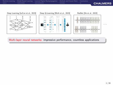
Deep Learning [LeCun et al., 2015] Deep Q-Learning [Mnih et al., 2015] ResNet [He et al., 2015]

· · ·

Multi-layer neural networks: impressive performance, countless applications

1 / 24

Machine Learning Model-Based Learning Learned Digital Backpropagation Outlook and Future Work Conclusions

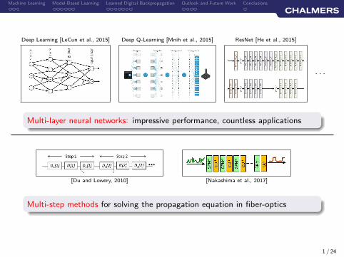
Deep Learning [LeCun et al., 2015] Deep Q-Learning [Mnih et al., 2015] ResNet [He et al., 2015]

· · ·

Multi-layer neural networks: impressive performance, countless applications

[Du and Lowery, 2010] [Nakashima et al., 2017]

Multi-step methods for solving the propagation equation in fiber-optics

1 / 24

Machine Learning Model-Based Learning Learned Digital Backpropagation Outlook and Future Work Conclusions

Agenda

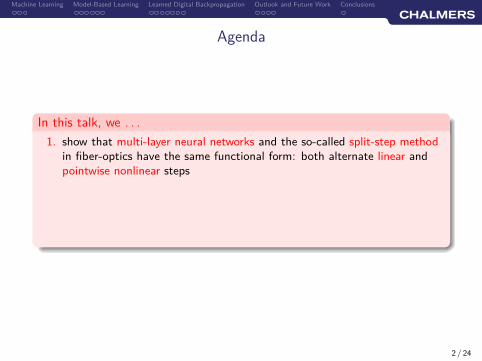
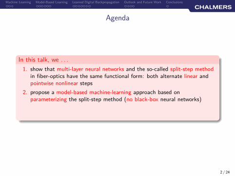
In this talk, we . . .

2 / 24

Machine Learning Model-Based Learning Learned Digital Backpropagation Outlook and Future Work Conclusions

Agenda

In this talk, we . . .

1. show that multi-layer neural networks and the so-called split-step methodin fiber-optics have the same functional form: both alternate linear andpointwise nonlinear steps

2 / 24

Machine Learning Model-Based Learning Learned Digital Backpropagation Outlook and Future Work Conclusions

Agenda

In this talk, we . . .

1. show that multi-layer neural networks and the so-called split-step methodin fiber-optics have the same functional form: both alternate linear andpointwise nonlinear steps

2. propose a model-based machine-learning approach based onparameterizing the split-step method (no black-box neural networks)

2 / 24

Machine Learning Model-Based Learning Learned Digital Backpropagation Outlook and Future Work Conclusions

Agenda

In this talk, we . . .

1. show that multi-layer neural networks and the so-called split-step methodin fiber-optics have the same functional form: both alternate linear andpointwise nonlinear steps

2. propose a model-based machine-learning approach based onparameterizing the split-step method (no black-box neural networks)

3. apply the proposed approach by revisiting hardware-efficient nonlinearequalization with deep-learning tools

2 / 24

Machine Learning Model-Based Learning Learned Digital Backpropagation Outlook and Future Work Conclusions

Outline

1. Machine Learning and Neural Networks for Communications

2. Model-Based Machine Learning for Fiber-Optic Systems

3. Nonlinear Equalization: Learned Digital Backpropagation

4. Outlook and Future Work

5. Conclusions

3 / 24

Machine Learning Model-Based Learning Learned Digital Backpropagation Outlook and Future Work Conclusions

Outline

1. Machine Learning and Neural Networks for Communications

2. Model-Based Machine Learning for Fiber-Optic Systems

3. Nonlinear Equalization: Learned Digital Backpropagation

4. Outlook and Future Work

5. Conclusions

4 / 24

Machine Learning Model-Based Learning Learned Digital Backpropagation Outlook and Future Work Conclusions

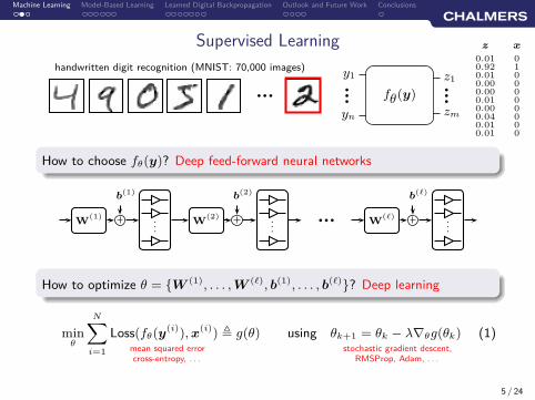
Supervised Learning

y1

yn

z1

zm

fθ(y)

parametersto be optimized/learned

bbb

bbb

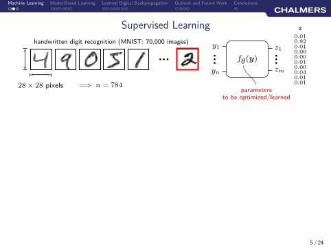
0.010.920.010.000.000.010.000.040.010.01

z

bbb

handwritten digit recognition (MNIST: 70,000 images)

28 × 28 pixels =⇒ n = 784

5 / 24

Machine Learning Model-Based Learning Learned Digital Backpropagation Outlook and Future Work Conclusions

Supervised Learning

y1

yn

z1

zm

fθ(y)bbb

bbb

0.010.920.010.000.000.010.000.040.010.01

z

bbb

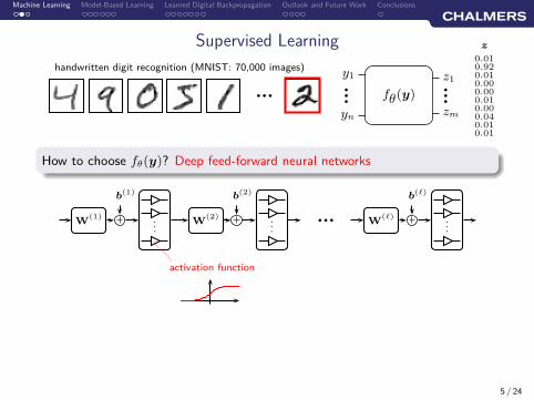
handwritten digit recognition (MNIST: 70,000 images)

How to choose fθ(y)? Deep feed-forward neural networks

W(1)

b(1)

.

.

.

activation function

W(2)

b(2)

.

.

.

bbbW

(ℓ)

b(ℓ)

.

.

.

5 / 24

Machine Learning Model-Based Learning Learned Digital Backpropagation Outlook and Future Work Conclusions

Supervised Learning

y1

yn

z1

zm

fθ(y)bbb

bbb

0100000000

x

0.010.920.010.000.000.010.000.040.010.01

z

bbb

handwritten digit recognition (MNIST: 70,000 images)

How to choose fθ(y)? Deep feed-forward neural networks

W(1)

b(1)

.

.

.W

(2)

b(2)

.

.

.

bbbW

(ℓ)

b(ℓ)

.

.

.

How to optimize θ = {W (1), . . . , W (ℓ), b(1), . . . , b(ℓ)}? Deep learning

minθ

N∑

i=1

Loss(fθ(y(i)), x(i)) , g(θ) using θk+1 = θk − λ∇θg(θk) (1)

5 / 24

mean squared errorcross-entropy, . . .

stochastic gradient descent,RMSProp, Adam, . . .

Machine Learning Model-Based Learning Learned Digital Backpropagation Outlook and Future Work Conclusions

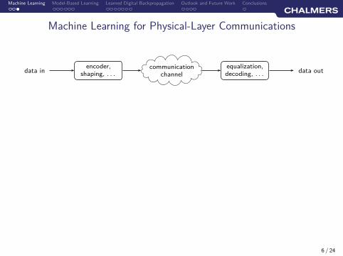
Machine Learning for Physical-Layer Communications

communicationchannel

data in data outencoder,

shaping, . . .equalization,decoding, . . .

6 / 24

Machine Learning Model-Based Learning Learned Digital Backpropagation Outlook and Future Work Conclusions

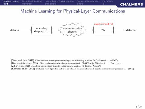
Machine Learning for Physical-Layer Communications

communicationchannel

data in data outencoder,

shaping, . . .

parameterized RX

Rθ

[Shen and Lau, 2011], Fiber nonlinearity compensation using extreme learning machine for DSP-based . . . , (OECC)

[Giacoumidis et al., 2015], Fiber nonlinearity-induced penalty reduction in CO-OFDM by ANN-based . . . , (Opt. Lett.)

[Zibar et al., 2016], Machine learning techniques in optical communication, (J. Lightw. Technol.)

[Kamalov et al., 2018], Evolution from 8qam live traffic to ps 64-qam with neural-network based nonlinearity compensation . . . , (OFC)

. . .

6 / 24

Machine Learning Model-Based Learning Learned Digital Backpropagation Outlook and Future Work Conclusions

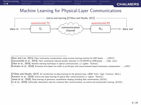
Machine Learning for Physical-Layer Communications

communicationchannel

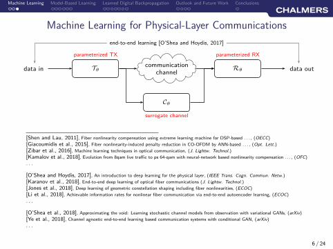
end-to-end learning [O’Shea and Hoydis, 2017]

data in data out

parameterized TX

Tθ

parameterized RX

Rθ

[Shen and Lau, 2011], Fiber nonlinearity compensation using extreme learning machine for DSP-based . . . , (OECC)

[Giacoumidis et al., 2015], Fiber nonlinearity-induced penalty reduction in CO-OFDM by ANN-based . . . , (Opt. Lett.)

[Zibar et al., 2016], Machine learning techniques in optical communication, (J. Lightw. Technol.)

[Kamalov et al., 2018], Evolution from 8qam live traffic to ps 64-qam with neural-network based nonlinearity compensation . . . , (OFC)

. . .

[O’Shea and Hoydis, 2017], An introduction to deep learning for the physical layer, (IEEE Trans. Cogn. Commun. Netw.)

[Karanov et al., 2018], End-to-end deep learning of optical fiber communications (J. Lightw. Technol.)

[Jones et al., 2018], Deep learning of geometric constellation shaping including fiber nonlinearities, (ECOC)

[Li et al., 2018], Achievable information rates for nonlinear fiber communication via end-to-end autoencoder learning, (ECOC)

. . .

6 / 24

Machine Learning Model-Based Learning Learned Digital Backpropagation Outlook and Future Work Conclusions

Machine Learning for Physical-Layer Communications

communicationchannel

end-to-end learning [O’Shea and Hoydis, 2017]

data in data out

parameterized TX

Tθ

parameterized RX

Rθ

Cθ

surrogate channel

[Shen and Lau, 2011], Fiber nonlinearity compensation using extreme learning machine for DSP-based . . . , (OECC)

[Giacoumidis et al., 2015], Fiber nonlinearity-induced penalty reduction in CO-OFDM by ANN-based . . . , (Opt. Lett.)

[Zibar et al., 2016], Machine learning techniques in optical communication, (J. Lightw. Technol.)

[Kamalov et al., 2018], Evolution from 8qam live traffic to ps 64-qam with neural-network based nonlinearity compensation . . . , (OFC)

. . .

[O’Shea and Hoydis, 2017], An introduction to deep learning for the physical layer, (IEEE Trans. Cogn. Commun. Netw.)

[Karanov et al., 2018], End-to-end deep learning of optical fiber communications (J. Lightw. Technol.)

[Jones et al., 2018], Deep learning of geometric constellation shaping including fiber nonlinearities, (ECOC)

[Li et al., 2018], Achievable information rates for nonlinear fiber communication via end-to-end autoencoder learning, (ECOC)

. . .

[O’Shea et al., 2018], Approximating the void: Learning stochastic channel models from observation with variational GANs, (arXiv)

[Ye et al., 2018], Channel agnostic end-to-end learning based communication systems with conditional GAN, (arXiv)

. . .

6 / 24

Machine Learning Model-Based Learning Learned Digital Backpropagation Outlook and Future Work Conclusions

Machine Learning for Physical-Layer Communications

communicationchannel

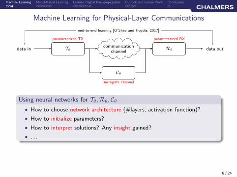
end-to-end learning [O’Shea and Hoydis, 2017]

data in data out

parameterized TX

Tθ

parameterized RX

Rθ

Cθ

surrogate channel

Using neural networks for Tθ, Rθ, Cθ

• How to choose network architecture (#layers, activation function)?

• How to initialize parameters?

• How to interpret solutions? Any insight gained?

• . . .

6 / 24

Machine Learning Model-Based Learning Learned Digital Backpropagation Outlook and Future Work Conclusions

Machine Learning for Physical-Layer Communications

communicationchannel

end-to-end learning [O’Shea and Hoydis, 2017]

data in data out

parameterized TX

Tθ

parameterized RX

Rθ

Cθ

surrogate channel

Using neural networks for Tθ, Rθ, Cθ

• How to choose network architecture (#layers, activation function)? ✗

• How to initialize parameters? ✗

• How to interpret solutions? Any insight gained? ✗

• . . .

Model-based learning: sparse signal recovery [Gregor and Lecun, 2010],

[Borgerding and Schniter, 2016], neural belief propagation [Nachmani et al., 2016],radio transformer networks [O’Shea and Hoydis, 2017], . . .

6 / 24

Machine Learning Model-Based Learning Learned Digital Backpropagation Outlook and Future Work Conclusions

Outline

1. Machine Learning and Neural Networks for Communications

2. Model-Based Machine Learning for Fiber-Optic Systems

3. Nonlinear Equalization: Learned Digital Backpropagation

4. Outlook and Future Work

5. Conclusions

7 / 24

Machine Learning Model-Based Learning Learned Digital Backpropagation Outlook and Future Work Conclusions

Fiber-Optic Communications

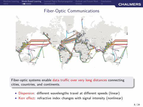
Fiber-optic systems enable data traffic over very long distances connectingcities, countries, and continents.

8 / 24

Machine Learning Model-Based Learning Learned Digital Backpropagation Outlook and Future Work Conclusions

Fiber-Optic Communications

Fiber-optic systems enable data traffic over very long distances connectingcities, countries, and continents.

• Dispersion: different wavelengths travel at different speeds (linear)

• Kerr effect: refractive index changes with signal intensity (nonlinear)

8 / 24

Machine Learning Model-Based Learning Learned Digital Backpropagation Outlook and Future Work Conclusions

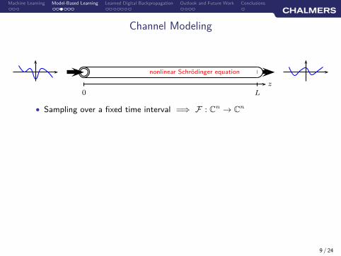
Channel Modeling

nonlinear Schrödinger equation

z

0 L

9 / 24

Machine Learning Model-Based Learning Learned Digital Backpropagation Outlook and Future Work Conclusions

Channel Modeling

nonlinear Schrödinger equation

z

0 L

• Sampling over a fixed time interval =⇒ F : Cn → Cn

9 / 24

Machine Learning Model-Based Learning Learned Digital Backpropagation Outlook and Future Work Conclusions

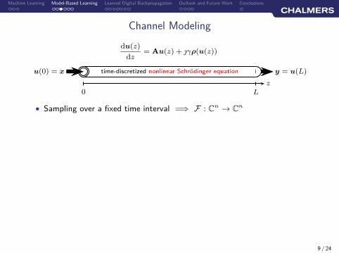
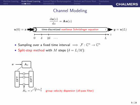
Channel Modeling

du(z)

dz= Au(z) + γρ(u(z))

time-discretized nonlinear Schrödinger equationu(0) = x y = u(L)

z

0 L

• Sampling over a fixed time interval =⇒ F : Cn → Cn

9 / 24

Machine Learning Model-Based Learning Learned Digital Backpropagation Outlook and Future Work Conclusions

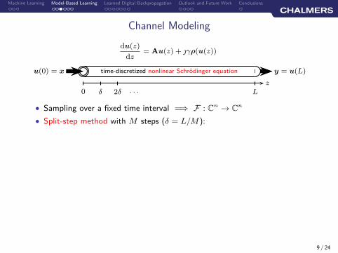
Channel Modeling

du(z)

dz= Au(z) + γρ(u(z))

time-discretized nonlinear Schrödinger equationu(0) = x y = u(L)

z

0 Lδ 2δ · · ·

• Sampling over a fixed time interval =⇒ F : Cn → Cn

• Split-step method with M steps (δ = L/M):

9 / 24

Machine Learning Model-Based Learning Learned Digital Backpropagation Outlook and Future Work Conclusions

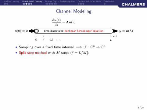
Channel Modeling

du(z)

dz= Au(z)

time-discretized nonlinear Schrödinger equationu(0) = x y = u(L)

z

0 Lδ 2δ · · ·

• Sampling over a fixed time interval =⇒ F : Cn → Cn

• Split-step method with M steps (δ = L/M):

9 / 24

Machine Learning Model-Based Learning Learned Digital Backpropagation Outlook and Future Work Conclusions

Channel Modeling

du(z)

dz= Au(z)

time-discretized nonlinear Schrödinger equationu(0) = x y = u(L)

z

0 Lδ 2δ · · ·

• Sampling over a fixed time interval =⇒ F : Cn → Cn

• Split-step method with M steps (δ = L/M):

Aδx

DF

T

.

.

. IDF

T

Hk = e

β22

δω2k group velocity dispersion (all-pass filter)

9 / 24

Machine Learning Model-Based Learning Learned Digital Backpropagation Outlook and Future Work Conclusions

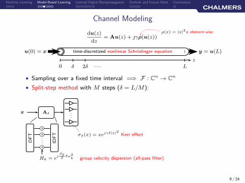
Channel Modeling

du(z)

dz= + γρ(u(z))

ρ(x) = |x|2x element-wise

time-discretized nonlinear Schrödinger equationu(0) = x y = u(L)

z

0 Lδ 2δ · · ·

• Sampling over a fixed time interval =⇒ F : Cn → Cn

• Split-step method with M steps (δ = L/M):

Aδx

DF

T

.

.

. IDF

T

Hk = e

β22

δω2k group velocity dispersion (all-pass filter)

9 / 24

Machine Learning Model-Based Learning Learned Digital Backpropagation Outlook and Future Work Conclusions

Channel Modeling

du(z)

dz= + γρ(u(z))

ρ(x) = |x|2x element-wise

time-discretized nonlinear Schrödinger equationu(0) = x y = u(L)

z

0 Lδ 2δ · · ·

• Sampling over a fixed time interval =⇒ F : Cn → Cn

• Split-step method with M steps (δ = L/M):

Aδx ...

σδ(x) = xeγδ|x|2

Kerr effect

DF

T

.

.

. IDF

T

Hk = e

β22

δω2k group velocity dispersion (all-pass filter)

9 / 24

Machine Learning Model-Based Learning Learned Digital Backpropagation Outlook and Future Work Conclusions

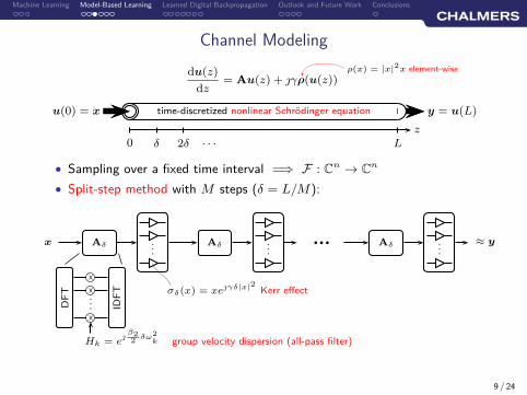
Channel Modeling

du(z)

dz= Au(z) + γρ(u(z))

ρ(x) = |x|2x element-wise

time-discretized nonlinear Schrödinger equationu(0) = x y = u(L)

z

0 Lδ 2δ · · ·

• Sampling over a fixed time interval =⇒ F : Cn → Cn

• Split-step method with M steps (δ = L/M):

Aδx ...

σδ(x) = xeγδ|x|2

Kerr effect

DF

T

.

.

. IDF

T

Hk = e

β22

δω2k group velocity dispersion (all-pass filter)

9 / 24

Machine Learning Model-Based Learning Learned Digital Backpropagation Outlook and Future Work Conclusions

Channel Modeling

du(z)

dz= Au(z) + γρ(u(z))

ρ(x) = |x|2x element-wise

time-discretized nonlinear Schrödinger equationu(0) = x y = u(L)

z

0 Lδ 2δ · · ·

• Sampling over a fixed time interval =⇒ F : Cn → Cn

• Split-step method with M steps (δ = L/M):

Aδx ...

σδ(x) = xeγδ|x|2

Kerr effect

DF

T

.

.

. IDF

T

Hk = e

β22

δω2k group velocity dispersion (all-pass filter)

Aδ ...

bbb Aδ ...

≈ y

9 / 24

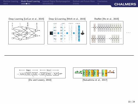
Machine Learning Model-Based Learning Learned Digital Backpropagation Outlook and Future Work Conclusions

Deep Learning [LeCun et al., 2015] Deep Q-Learning [Mnih et al., 2015] ResNet [He et al., 2015]

· · ·

[Du and Lowery, 2010] [Nakashima et al., 2017]

10 / 24

Machine Learning Model-Based Learning Learned Digital Backpropagation Outlook and Future Work Conclusions

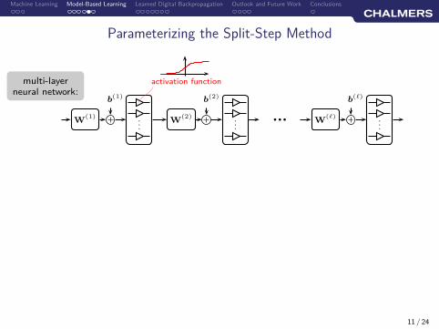
Parameterizing the Split-Step Method

multi-layerneural network:

W(1)

b(1)

.

.

.

activation function

W(2)

b(2)

.

.

.

bbbW

(ℓ)

b(ℓ)

.

.

.

11 / 24

Machine Learning Model-Based Learning Learned Digital Backpropagation Outlook and Future Work Conclusions

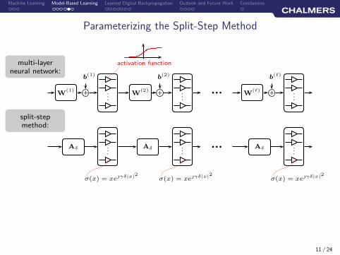
Parameterizing the Split-Step Method

multi-layerneural network:

W(1)

b(1)

.

.

.

activation function

W(2)

b(2)

.

.

.

bbbW

(ℓ)

b(ℓ)

.

.

.

split-stepmethod:

Aδ ...

σ(x) = xeγδ|x|2

Aδ ...

σ(x) = xeγδ|x|2

bbb Aδ ...

σ(x) = xeγδ|x|2

11 / 24

Machine Learning Model-Based Learning Learned Digital Backpropagation Outlook and Future Work Conclusions

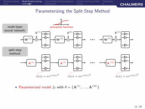
Parameterizing the Split-Step Method

multi-layerneural network:

W(1)

b(1)

.

.

.

activation function

W(2)

b(2)

.

.

.

bbbW

(ℓ)

b(ℓ)

.

.

.

split-stepmethod:

A(1) .

.

.

σ(x) = xeγδ|x|2

A(2) .

.

.

σ(x) = xeγδ|x|2

bbbA

(M) ...

σ(x) = xeγδ|x|2

[Häger & Pfister, 2018], Nonlinear Interference Mitigation via Deep Neural Networks, (OFC)

[Häger & Pfister, 2018], Deep Learning of the Nonlinear Schrödinger Equation in Fiber-Optic Communications, (ISIT)

11 / 24

Machine Learning Model-Based Learning Learned Digital Backpropagation Outlook and Future Work Conclusions

Parameterizing the Split-Step Method

multi-layerneural network:

W(1)

b(1)

.

.

.

activation function

W(2)

b(2)

.

.

.

bbbW

(ℓ)

b(ℓ)

.

.

.

split-stepmethod:

A(1) .

.

.

σ(x) = xeγδ|x|2

A(2) .

.

.

σ(x) = xeγδ|x|2

bbbA

(M) ...

σ(x) = xeγδ|x|2

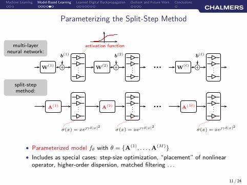
• Parameterized model fθ with θ = {A(1), . . . , A

(M)}

11 / 24

Machine Learning Model-Based Learning Learned Digital Backpropagation Outlook and Future Work Conclusions

Parameterizing the Split-Step Method

multi-layerneural network:

W(1)

b(1)

.

.

.

activation function

W(2)

b(2)

.

.

.

bbbW

(ℓ)

b(ℓ)

.

.

.

split-stepmethod:

A(1) .

.

.

σ(x) = xeγδ|x|2

A(2) .

.

.

σ(x) = xeγδ|x|2

bbbA

(M) ...

σ(x) = xeγδ|x|2

• Parameterized model fθ with θ = {A(1), . . . , A

(M)}

• Includes as special cases: step-size optimization, “placement” of nonlinearoperator, higher-order dispersion, matched filtering . . .

11 / 24

Machine Learning Model-Based Learning Learned Digital Backpropagation Outlook and Future Work Conclusions

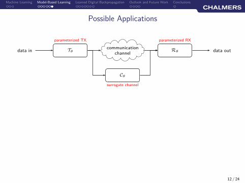
Possible Applications

communicationchannel

data in data out

parameterized TX

Tθ

parameterized RX

Rθ

Cθ

surrogate channel

12 / 24

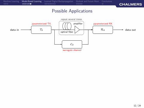
Machine Learning Model-Based Learning Learned Digital Backpropagation Outlook and Future Work Conclusions

Possible Applications

optical fiber

amplifier

repeat several times

data in data out

parameterized TX

Tθ

parameterized RX

Rθ

Cθ

surrogate channel

12 / 24

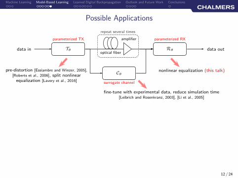
Machine Learning Model-Based Learning Learned Digital Backpropagation Outlook and Future Work Conclusions

Possible Applications

optical fiber

amplifier

repeat several times

data in data out

parameterized TX

Tθ

parameterized RX

Rθ

Cθ

surrogate channel

pre-distortion [Essiambre and Winzer, 2005],

[Roberts et al., 2006], split nonlinearequalization [Lavery et al., 2016]

nonlinear equalization (this talk)

fine-tune with experimental data, reduce simulation time[Leibrich and Rosenkranz, 2003], [Li et al., 2005]

12 / 24

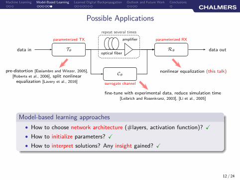
Machine Learning Model-Based Learning Learned Digital Backpropagation Outlook and Future Work Conclusions

Possible Applications

optical fiber

amplifier

repeat several times

data in data out

parameterized TX

Tθ

parameterized RX

Rθ

Cθ

surrogate channel

pre-distortion [Essiambre and Winzer, 2005],

[Roberts et al., 2006], split nonlinearequalization [Lavery et al., 2016]

nonlinear equalization (this talk)

fine-tune with experimental data, reduce simulation time[Leibrich and Rosenkranz, 2003], [Li et al., 2005]

Model-based learning approaches

• How to choose network architecture (#layers, activation function)? X

• How to initialize parameters? X

• How to interpret solutions? Any insight gained? X

12 / 24

Machine Learning Model-Based Learning Learned Digital Backpropagation Outlook and Future Work Conclusions

Outline

1. Machine Learning and Neural Networks for Communications

2. Model-Based Machine Learning for Fiber-Optic Systems

3. Nonlinear Equalization: Learned Digital Backpropagation

4. Outlook and Future Work

5. Conclusions

13 / 24

Machine Learning Model-Based Learning Learned Digital Backpropagation Outlook and Future Work Conclusions

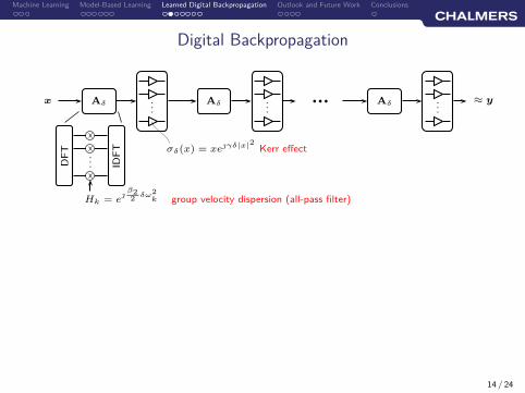
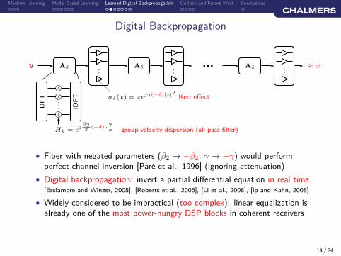
Digital Backpropagation

Aδx ...

σδ(x) = xeγδ|x|2

Kerr effect

DF

T

.

.

. IDF

T

Hk = e

β22

δω2k group velocity dispersion (all-pass filter)

Aδ ...

bbb Aδ ...

≈ y

14 / 24

Machine Learning Model-Based Learning Learned Digital Backpropagation Outlook and Future Work Conclusions

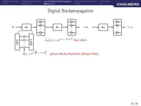
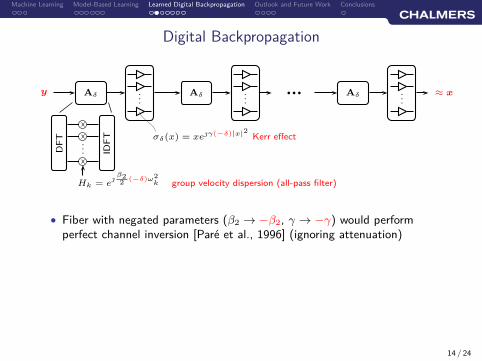
Digital Backpropagation

Aδy ...

σδ(x) = xeγ(−δ)|x|2

Kerr effect

DF

T

.

.

. IDF

T

Hk = e

β22

(−δ)ω2k group velocity dispersion (all-pass filter)

Aδ ...

bbb Aδ ...

≈ x

14 / 24

Machine Learning Model-Based Learning Learned Digital Backpropagation Outlook and Future Work Conclusions

Digital Backpropagation

Aδy ...

σδ(x) = xeγ(−δ)|x|2

Kerr effect

DF

T

.

.

. IDF

T

Hk = e

β22

(−δ)ω2k group velocity dispersion (all-pass filter)

Aδ ...

bbb Aδ ...

≈ x

• Fiber with negated parameters (β2 → −β2, γ → −γ) would performperfect channel inversion [Paré et al., 1996] (ignoring attenuation)

14 / 24

Machine Learning Model-Based Learning Learned Digital Backpropagation Outlook and Future Work Conclusions

Digital Backpropagation

Aδy ...

σδ(x) = xeγ(−δ)|x|2

Kerr effect

DF

T

.

.

. IDF

T

Hk = e

β22

(−δ)ω2k group velocity dispersion (all-pass filter)

Aδ ...

bbb Aδ ...

≈ x

• Fiber with negated parameters (β2 → −β2, γ → −γ) would performperfect channel inversion [Paré et al., 1996] (ignoring attenuation)

• Digital backpropagation: invert a partial differential equation in real time[Essiambre and Winzer, 2005], [Roberts et al., 2006], [Li et al., 2008], [Ip and Kahn, 2008]

14 / 24

Machine Learning Model-Based Learning Learned Digital Backpropagation Outlook and Future Work Conclusions

Digital Backpropagation

Aδy ...

σδ(x) = xeγ(−δ)|x|2

Kerr effect

DF

T

.

.

. IDF

T

Hk = e

β22

(−δ)ω2k group velocity dispersion (all-pass filter)

Aδ ...

bbb Aδ ...

≈ x

• Fiber with negated parameters (β2 → −β2, γ → −γ) would performperfect channel inversion [Paré et al., 1996] (ignoring attenuation)

• Digital backpropagation: invert a partial differential equation in real time[Essiambre and Winzer, 2005], [Roberts et al., 2006], [Li et al., 2008], [Ip and Kahn, 2008]

• Widely considered to be impractical (too complex): linear equalization isalready one of the most power-hungry DSP blocks in coherent receivers

14 / 24

Machine Learning Model-Based Learning Learned Digital Backpropagation Outlook and Future Work Conclusions

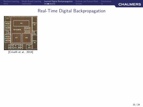
Real-Time Digital Backpropagation

[Crivelli et al., 2014]

15 / 24

Machine Learning Model-Based Learning Learned Digital Backpropagation Outlook and Future Work Conclusions

Real-Time Digital Backpropagation

[Crivelli et al., 2014]

15 / 24

Machine Learning Model-Based Learning Learned Digital Backpropagation Outlook and Future Work Conclusions

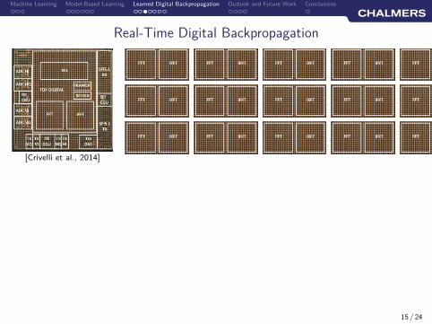
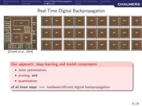
Real-Time Digital Backpropagation

[Crivelli et al., 2014]

Our approach: deep learning and model compression

• Joint optimization,

• pruning, and

• quantization

of all linear steps =⇒ hardware-efficient digital backpropagation

15 / 24

Machine Learning Model-Based Learning Learned Digital Backpropagation Outlook and Future Work Conclusions

Learned Digital Backpropagation

16 / 24

Machine Learning Model-Based Learning Learned Digital Backpropagation Outlook and Future Work Conclusions

Learned Digital Backpropagation

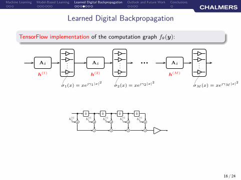
TensorFlow implementation of the computation graph fθ(y):

h(1) h(2) h(M)

Aδ ...

σ1(x) = xeγ1|x|2

Aδ ...

σ2(x) = xeγ2|x|2

bbb Aδ ...

σM (x) = xeγM |x|2

h(i)2

b D

h(i)1

b D

h(i)0

b D

h(i)1

b D

h(i)2

16 / 24

Machine Learning Model-Based Learning Learned Digital Backpropagation Outlook and Future Work Conclusions

Learned Digital Backpropagation

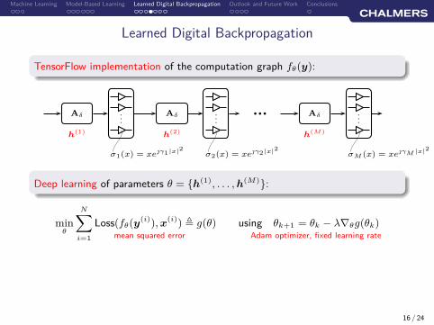
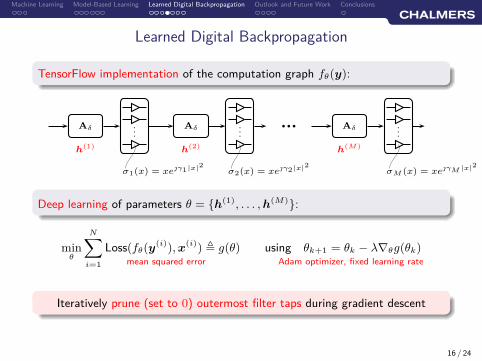
TensorFlow implementation of the computation graph fθ(y):

h(1) h(2) h(M)

Aδ ...

σ1(x) = xeγ1|x|2

Aδ ...

σ2(x) = xeγ2|x|2

bbb Aδ ...

σM (x) = xeγM |x|2

mean squared error Adam optimizer, fixed learning rate

Deep learning of parameters θ = {h(1), . . . , h(M)}:

minθ

N∑

i=1

Loss(fθ(y(i)), x(i)) , g(θ) using θk+1 = θk − λ∇θg(θk)

16 / 24

Machine Learning Model-Based Learning Learned Digital Backpropagation Outlook and Future Work Conclusions

Learned Digital Backpropagation

TensorFlow implementation of the computation graph fθ(y):

h(1) h(2) h(M)

Aδ ...

σ1(x) = xeγ1|x|2

Aδ ...

σ2(x) = xeγ2|x|2

bbb Aδ ...

σM (x) = xeγM |x|2

mean squared error Adam optimizer, fixed learning rate

Deep learning of parameters θ = {h(1), . . . , h(M)}:

minθ

N∑

i=1

Loss(fθ(y(i)), x(i)) , g(θ) using θk+1 = θk − λ∇θg(θk)

Iteratively prune (set to 0) outermost filter taps during gradient descent

16 / 24

Machine Learning Model-Based Learning Learned Digital Backpropagation Outlook and Future Work Conclusions

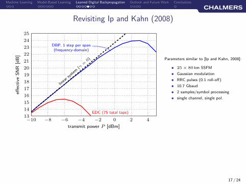
Revisiting Ip and Kahn (2008)

13

14

15

16

17

18

19

20

21

22

23

24

25

−10 −8 −6 −4 −2 0 2 4

transmit power P [dBm]

effec

tive

SN

R[d

B]

linea

r syst

em(γ

=0)

EDC (75 total taps)

DBP, 1 step per span(frequency-domain)

Parameters similar to [Ip and Kahn, 2008]:

• 25 × 80 km SSFM

• Gaussian modulation

• RRC pulses (0.1 roll-off)

• 10.7 Gbaud

• 2 samples/symbol processing

• single channel, single pol.

17 / 24

Machine Learning Model-Based Learning Learned Digital Backpropagation Outlook and Future Work Conclusions

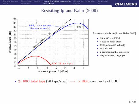
Revisiting Ip and Kahn (2008)

13

14

15

16

17

18

19

20

21

22

23

24

25

−10 −8 −6 −4 −2 0 2 4

transmit power P [dBm]

effec

tive

SN

R[d

B]

linea

r syst

em(γ

=0)

EDC (75 total taps)

DBP, 1 step per span(frequency-domain)

2 dB

Parameters similar to [Ip and Kahn, 2008]:

• 25 × 80 km SSFM

• Gaussian modulation

• RRC pulses (0.1 roll-off)

• 10.7 Gbaud

• 2 samples/symbol processing

• single channel, single pol.

• ≫ 1000 total taps (70 taps/step) =⇒ > 100× complexity of EDC

17 / 24

Machine Learning Model-Based Learning Learned Digital Backpropagation Outlook and Future Work Conclusions

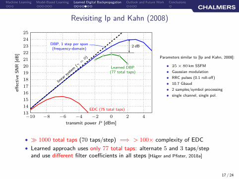
Revisiting Ip and Kahn (2008)

13

14

15

16

17

18

19

20

21

22

23

24

25

−10 −8 −6 −4 −2 0 2 4

transmit power P [dBm]

effec

tive

SN

R[d

B]

uTuT uT uT

uT

linea

r syst

em(γ

=0)

EDC (75 total taps)

Learned DBP(77 total taps)

DBP, 1 step per span(frequency-domain)

2 dB

Parameters similar to [Ip and Kahn, 2008]:

• 25 × 80 km SSFM

• Gaussian modulation

• RRC pulses (0.1 roll-off)

• 10.7 Gbaud

• 2 samples/symbol processing

• single channel, single pol.

• ≫ 1000 total taps (70 taps/step) =⇒ > 100× complexity of EDC

• Learned approach uses only 77 total taps: alternate 5 and 3 taps/stepand use different filter coefficients in all steps [Häger and Pfister, 2018a]

17 / 24

Machine Learning Model-Based Learning Learned Digital Backpropagation Outlook and Future Work Conclusions

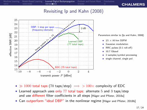
Revisiting Ip and Kahn (2008)

13

14

15

16

17

18

19

20

21

22

23

24

25

−10 −8 −6 −4 −2 0 2 4

transmit power P [dBm]

effec

tive

SN

R[d

B]

uTuT uT uT

uT

linea

r syst

em(γ

=0)

EDC (75 total taps)

Learned DBP(77 total taps)

DBP, 1 step per span(frequency-domain)

2 dB

Parameters similar to [Ip and Kahn, 2008]:

• 25 × 80 km SSFM

• Gaussian modulation

• RRC pulses (0.1 roll-off)

• 10.7 Gbaud

• 2 samples/symbol processing

• single channel, single pol.

• ≫ 1000 total taps (70 taps/step) =⇒ > 100× complexity of EDC

• Learned approach uses only 77 total taps: alternate 5 and 3 taps/stepand use different filter coefficients in all steps [Häger and Pfister, 2018a]

• Can outperform “ideal DBP” in the nonlinear regime [Häger and Pfister, 2018b]

17 / 24

Machine Learning Model-Based Learning Learned Digital Backpropagation Outlook and Future Work Conclusions

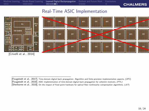
Real-Time ASIC Implementation

[Crivelli et al., 2014]

18 / 24

Machine Learning Model-Based Learning Learned Digital Backpropagation Outlook and Future Work Conclusions

Real-Time ASIC Implementation

[Crivelli et al., 2014]

[Fougstedt et al., 2017], Time-domain digital back propagation: Algorithm and finite-precision implementation aspects, (OFC)

[Fougstedt et al., 2018], ASIC implementation of time-domain digital back propagation for coherent receivers, (PTL)

[Sherborne et al., 2018], On the impact of fixed point hardware for optical fiber nonlinearity compensation algorithms, (JLT)

18 / 24

Machine Learning Model-Based Learning Learned Digital Backpropagation Outlook and Future Work Conclusions

Real-Time ASIC Implementation

[Crivelli et al., 2014]

h(i)1

b D

h(i)0

b D

h(i)1

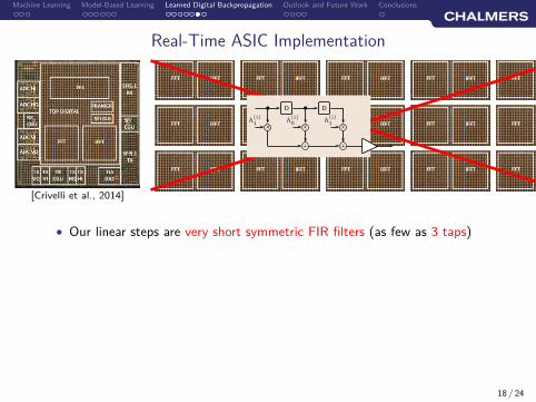
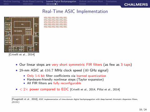
• Our linear steps are very short symmetric FIR filters (as few as 3 taps)

18 / 24

Machine Learning Model-Based Learning Learned Digital Backpropagation Outlook and Future Work Conclusions

Real-Time ASIC Implementation

[Crivelli et al., 2014]

h(i)1

b D

h(i)0

b D

h(i)1 h

(i)1

b D

h(i)0

b D

h(i)1 h

(i)1

b D

h(i)0

b D

h(i)1 h

(i)1

b D

h(i)0

b D

h(i)1 h

(i)1

b D

h(i)0

b D

h(i)1

h(i)1

b D

h(i)0

b D

h(i)1 h

(i)1

b D

h(i)0

b D

h(i)1 h

(i)1

b D

h(i)0

b D

h(i)1 h

(i)1

b D

h(i)0

b D

h(i)1 h

(i)1

b D

h(i)0

b D

h(i)1

h(i)1

b D

h(i)0

b D

h(i)1 h

(i)1

b D

h(i)0

b D

h(i)1 h

(i)1

b D

h(i)0

b D

h(i)1 h

(i)1

b D

h(i)0

b D

h(i)1 h

(i)1

b D

h(i)0

b D

h(i)1

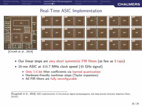
• Our linear steps are very short symmetric FIR filters (as few as 3 taps)

• 28-nm ASIC at 416.7 MHz clock speed (40 GHz signal)

• Only 5-6 bit filter coefficients via learned quantization• Hardware-friendly nonlinear steps (Taylor expansion)• All FIR filters are fully reconfigurable

[Fougstedt et al., 2018], ASIC implementation of time-domain digital backpropagation with deep-learned chromatic dispersion filters,

(ECOC)

18 / 24

Machine Learning Model-Based Learning Learned Digital Backpropagation Outlook and Future Work Conclusions

Real-Time ASIC Implementation

[Crivelli et al., 2014]

h(i)1

b D

h(i)0

b D

h(i)1 h

(i)1

b D

h(i)0

b D

h(i)1 h

(i)1

b D

h(i)0

b D

h(i)1 h

(i)1

b D

h(i)0

b D

h(i)1 h

(i)1

b D

h(i)0

b D

h(i)1

h(i)1

b D

h(i)0

b D

h(i)1 h

(i)1

b D

h(i)0

b D

h(i)1 h

(i)1

b D

h(i)0

b D

h(i)1 h

(i)1

b D

h(i)0

b D

h(i)1 h

(i)1

b D

h(i)0

b D

h(i)1

h(i)1

b D

h(i)0

b D

h(i)1 h

(i)1

b D

h(i)0

b D

h(i)1 h

(i)1

b D

h(i)0

b D

h(i)1 h

(i)1

b D

h(i)0

b D

h(i)1 h

(i)1

b D

h(i)0

b D

h(i)1

• Our linear steps are very short symmetric FIR filters (as few as 3 taps)

• 28-nm ASIC at 416.7 MHz clock speed (40 GHz signal)

• Only 5-6 bit filter coefficients via learned quantization• Hardware-friendly nonlinear steps (Taylor expansion)• All FIR filters are fully reconfigurable

[Fougstedt et al., 2018], ASIC implementation of time-domain digital backpropagation with deep-learned chromatic dispersion filters,

(ECOC)

18 / 24

Machine Learning Model-Based Learning Learned Digital Backpropagation Outlook and Future Work Conclusions

Real-Time ASIC Implementation

[Crivelli et al., 2014]

h(i)1

b D

h(i)0

b D

h(i)1 h

(i)1

b D

h(i)0

b D

h(i)1 h

(i)1

b D

h(i)0

b D

h(i)1 h

(i)1

b D

h(i)0

b D

h(i)1 h

(i)1

b D

h(i)0

b D

h(i)1 h

(i)1

b D

h(i)0

b D

h(i)1

h(i)1

b D

h(i)0

b D

h(i)1 h

(i)1

b D

h(i)0

b D

h(i)1 h

(i)1

b D

h(i)0

b D

h(i)1 h

(i)1

b D

h(i)0

b D

h(i)1 h

(i)1

b D

h(i)0

b D

h(i)1 h

(i)1

b D

h(i)0

b D

h(i)1

h(i)1

b D

h(i)0

b D

h(i)1 h

(i)1

b D

h(i)0

b D

h(i)1 h

(i)1

b D

h(i)0

b D

h(i)1 h

(i)1

b D

h(i)0

b D

h(i)1 h

(i)1

b D

h(i)0

b D

h(i)1 h

(i)1

b D

h(i)0

b D

h(i)1

h(i)1

b D

h(i)0

b D

h(i)1 h

(i)1

b D

h(i)0

b D

h(i)1 h

(i)1

b D

h(i)0

b D

h(i)1 h

(i)1

b D

h(i)0

b D

h(i)1 h

(i)1

b D

h(i)0

b D

h(i)1 h

(i)1

b D

h(i)0

b D

h(i)1

h(i)1

b D

h(i)0

b D

h(i)1 h

(i)1

b D

h(i)0

b D

h(i)1 h

(i)1

b D

h(i)0

b D

h(i)1 h

(i)1

b D

h(i)0

b D

h(i)1 h

(i)1

b D

h(i)0

b D

h(i)1 h

(i)1

b D

h(i)0

b D

h(i)1

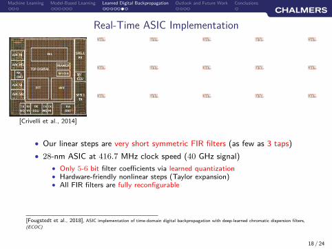
• Our linear steps are very short symmetric FIR filters (as few as 3 taps)

• 28-nm ASIC at 416.7 MHz clock speed (40 GHz signal)

• Only 5-6 bit filter coefficients via learned quantization• Hardware-friendly nonlinear steps (Taylor expansion)• All FIR filters are fully reconfigurable

• < 2× power compared to EDC [Crivelli et al., 2014, Pillai et al., 2014]

[Fougstedt et al., 2018], ASIC implementation of time-domain digital backpropagation with deep-learned chromatic dispersion filters,

(ECOC)

18 / 24

Machine Learning Model-Based Learning Learned Digital Backpropagation Outlook and Future Work Conclusions

Why Does The Learning Approach Work?

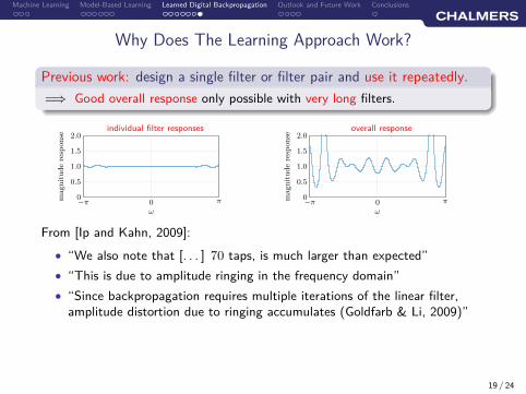
Previous work: design a single filter or filter pair and use it repeatedly.

=⇒ Good overall response only possible with very long filters.

individual filter responses

0

0.5

1.0

1.5

2.0

ω

magnituderesp

onse

0 π−π

overall response

0

0.5

1.0

1.5

2.0

ω

magnituderesp

onse

0 π−π

From [Ip and Kahn, 2009]:

• “We also note that [. . . ] 70 taps, is much larger than expected”

• “This is due to amplitude ringing in the frequency domain”

• “Since backpropagation requires multiple iterations of the linear filter,amplitude distortion due to ringing accumulates (Goldfarb & Li, 2009)”

19 / 24

Machine Learning Model-Based Learning Learned Digital Backpropagation Outlook and Future Work Conclusions

Why Does The Learning Approach Work?

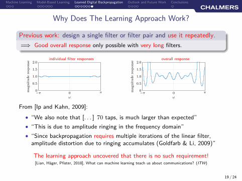
Previous work: design a single filter or filter pair and use it repeatedly.

=⇒ Good overall response only possible with very long filters.

individual filter responses

0

0.5

1.0

1.5

2.0

ω

magnituderesp

onse

0 π−π

overall response

0

0.5

1.0

1.5

2.0

ω

magnituderesp

onse

0 π−π

From [Ip and Kahn, 2009]:

• “We also note that [. . . ] 70 taps, is much larger than expected”

• “This is due to amplitude ringing in the frequency domain”

• “Since backpropagation requires multiple iterations of the linear filter,amplitude distortion due to ringing accumulates (Goldfarb & Li, 2009)”

The learning approach uncovered that there is no such requirement![Lian, Häger, Pfister, 2018], What can machine learning teach us about communications? (ITW)

19 / 24

Machine Learning Model-Based Learning Learned Digital Backpropagation Outlook and Future Work Conclusions

Why Does The Learning Approach Work?

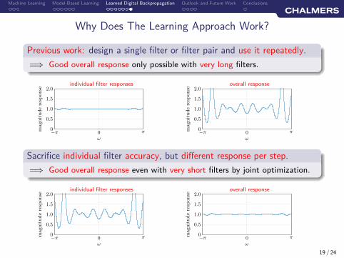
Previous work: design a single filter or filter pair and use it repeatedly.

=⇒ Good overall response only possible with very long filters.

individual filter responses

0

0.5

1.0

1.5

2.0

ω

magnituderesp

onse

0 π−π

overall response

0

0.5

1.0

1.5

2.0

ω

magnituderesp

onse

0 π−π

Sacrifice individual filter accuracy, but different response per step.

=⇒ Good overall response even with very short filters by joint optimization.

individual filter responses

0

0.5

1.0

1.5

2.0

ω

magnituderesp

onse

0 π−π

overall response

0

0.5

1.0

1.5

2.0

ω

magnituderesp

onse

0 π−π

19 / 24

Machine Learning Model-Based Learning Learned Digital Backpropagation Outlook and Future Work Conclusions

Outline

1. Machine Learning and Neural Networks for Communications

2. Model-Based Machine Learning for Fiber-Optic Systems

3. Nonlinear Equalization: Learned Digital Backpropagation

4. Outlook and Future Work

5. Conclusions

20 / 24

Machine Learning Model-Based Learning Learned Digital Backpropagation Outlook and Future Work Conclusions

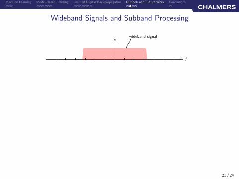
Wideband Signals and Subband Processing

.

f

wideband signal

21 / 24

Machine Learning Model-Based Learning Learned Digital Backpropagation Outlook and Future Work Conclusions

Wideband Signals and Subband Processing

.

f

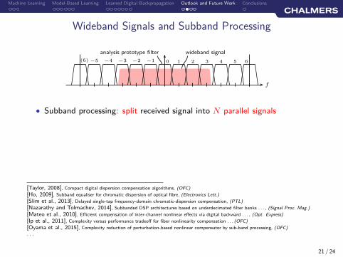
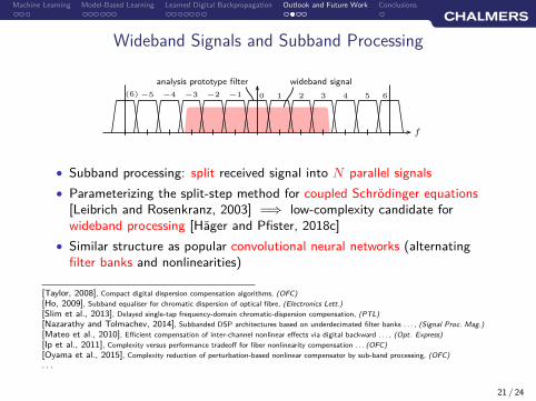
1 2 3 4 5−5 −4 −3 −2 −1 0 6(6)

analysis prototype filter wideband signal

• Subband processing: split received signal into N parallel signals

[Taylor, 2008], Compact digital dispersion compensation algorithms, (OFC)

[Ho, 2009], Subband equaliser for chromatic dispersion of optical fibre, (Electronics Lett.)

[Slim et al., 2013], Delayed single-tap frequency-domain chromatic-dispersion compensation, (PTL)

[Nazarathy and Tolmachev, 2014], Subbanded DSP architectures based on underdecimated filter banks . . . , (Signal Proc. Mag.)

[Mateo et al., 2010], Efficient compensation of inter-channel nonlinear effects via digital backward . . . , (Opt. Express)

[Ip et al., 2011], Complexity versus performance tradeoff for fiber nonlinearity compensation . . . (OFC)

[Oyama et al., 2015], Complexity reduction of perturbation-based nonlinear compensator by sub-band processing, (OFC)

. . .

21 / 24

Machine Learning Model-Based Learning Learned Digital Backpropagation Outlook and Future Work Conclusions

Wideband Signals and Subband Processing

.

f

1 2 3 4 5−5 −4 −3 −2 −1 0 6(6)

analysis prototype filter wideband signal

• Subband processing: split received signal into N parallel signals

• Parameterizing the split-step method for coupled Schrödinger equations[Leibrich and Rosenkranz, 2003] =⇒ low-complexity candidate forwideband processing [Häger and Pfister, 2018c]

• Similar structure as popular convolutional neural networks (alternatingfilter banks and nonlinearities)

[Taylor, 2008], Compact digital dispersion compensation algorithms, (OFC)

[Ho, 2009], Subband equaliser for chromatic dispersion of optical fibre, (Electronics Lett.)

[Slim et al., 2013], Delayed single-tap frequency-domain chromatic-dispersion compensation, (PTL)

[Nazarathy and Tolmachev, 2014], Subbanded DSP architectures based on underdecimated filter banks . . . , (Signal Proc. Mag.)

[Mateo et al., 2010], Efficient compensation of inter-channel nonlinear effects via digital backward . . . , (Opt. Express)

[Ip et al., 2011], Complexity versus performance tradeoff for fiber nonlinearity compensation . . . (OFC)

[Oyama et al., 2015], Complexity reduction of perturbation-based nonlinear compensator by sub-band processing, (OFC)

. . .

21 / 24

Machine Learning Model-Based Learning Learned Digital Backpropagation Outlook and Future Work Conclusions

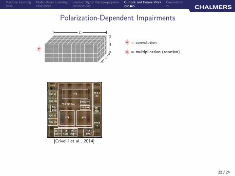
Polarization-Dependent Impairments

∗

4

4

L

× = multiplication (rotation)

∗ = convolution

[Crivelli et al., 2014]

22 / 24

Machine Learning Model-Based Learning Learned Digital Backpropagation Outlook and Future Work Conclusions

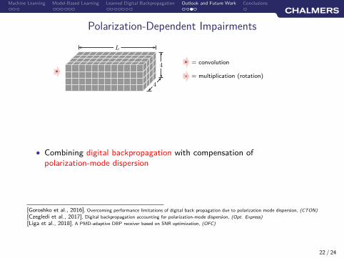
Polarization-Dependent Impairments

∗

4

4

L

× = multiplication (rotation)

∗ = convolution

• Combining digital backpropagation with compensation ofpolarization-mode dispersion

[Goroshko et al., 2016], Overcoming performance limitations of digital back propagation due to polarization mode dispersion, (CTON)

[Czegledi et al., 2017], Digital backpropagation accounting for polarization-mode dispersion, (Opt. Express)

[Liga et al., 2018], A PMD-adaptive DBP receiver based on SNR optimization, (OFC)

22 / 24

Machine Learning Model-Based Learning Learned Digital Backpropagation Outlook and Future Work Conclusions

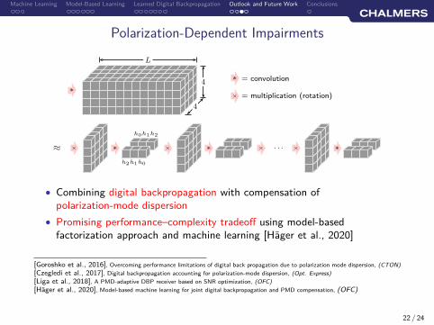
Polarization-Dependent Impairments

∗

4

4

L

× = multiplication (rotation)

∗ = convolution

≈ ×

h2h1h0

h0h1h2

∗ × ∗ × . . . × ∗

• Combining digital backpropagation with compensation ofpolarization-mode dispersion

• Promising performance–complexity tradeoff using model-basedfactorization approach and machine learning [Häger et al., 2020]

[Goroshko et al., 2016], Overcoming performance limitations of digital back propagation due to polarization mode dispersion, (CTON)

[Czegledi et al., 2017], Digital backpropagation accounting for polarization-mode dispersion, (Opt. Express)

[Liga et al., 2018], A PMD-adaptive DBP receiver based on SNR optimization, (OFC)

[Häger et al., 2020], Model-based machine learning for joint digital backpropagation and PMD compensation, (OFC)

22 / 24

Machine Learning Model-Based Learning Learned Digital Backpropagation Outlook and Future Work Conclusions

Ongoing and Future Work

• Experimental Demonstrations: stay tuned . . .

• How to integrate into a standard coherent receiver DSP chain?

• How to successfully train in the presence of practical impairments (laserphase noise, transceiver noise, . . . )

• How realistic is online learning in custom DSP? (We only have “hundreds”of parameters, not “thousands” or “millions” like neural networks)

23 / 24

Machine Learning Model-Based Learning Learned Digital Backpropagation Outlook and Future Work Conclusions

Conclusions

24 / 24

Machine Learning Model-Based Learning Learned Digital Backpropagation Outlook and Future Work Conclusions

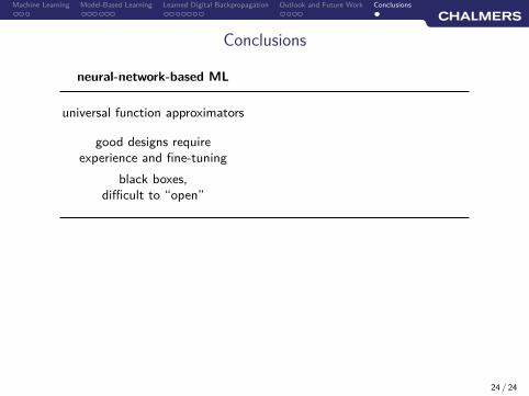
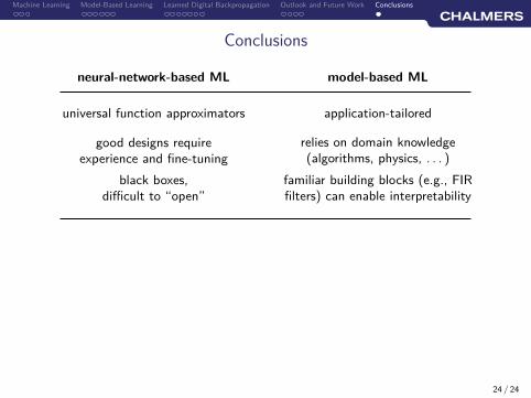
Conclusions

neural-network-based ML

universal function approximators

good designs requireexperience and fine-tuning

black boxes,difficult to “open”

24 / 24

Machine Learning Model-Based Learning Learned Digital Backpropagation Outlook and Future Work Conclusions

Conclusions

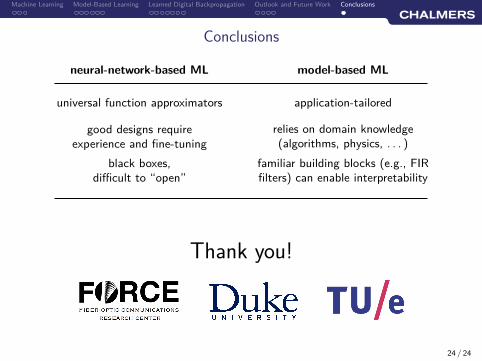
neural-network-based ML model-based ML

universal function approximators application-tailored

good designs requireexperience and fine-tuning

relies on domain knowledge(algorithms, physics, . . . )

black boxes,difficult to “open”

familiar building blocks (e.g., FIRfilters) can enable interpretability

24 / 24

Machine Learning Model-Based Learning Learned Digital Backpropagation Outlook and Future Work Conclusions

Conclusions

neural-network-based ML model-based ML

universal function approximators application-tailored

good designs requireexperience and fine-tuning

relies on domain knowledge(algorithms, physics, . . . )

black boxes,difficult to “open”

familiar building blocks (e.g., FIRfilters) can enable interpretability

Thank you!

24 / 24

References I

Borgerding, M. and Schniter, P. (2016).

Onsager-corrected deep learning for sparse linear inverse problems.In Proc. IEEE Global Conf. Signal and Information Processing (GlobalSIP), Washington, DC.

Crivelli, D. E., Hueda, M. R., Carrer, H. S., Del Barco, M., López, R. R., Gianni, P., Finochietto, J.,

Swenson, N., Voois, P., and Agazzi, O. E. (2014).Architecture of a single-chip 50 Gb/s DP-QPSK/BPSK transceiver with electronic dispersion compensationfor coherent optical channels.IEEE Trans. Circuits Syst. I: Reg. Papers, 61(4):1012–1025.

Du, L. B. and Lowery, A. J. (2010).

Improved single channel backpropagation for intra-channel fiber nonlinearity compensation in long-hauloptical communication systems.Opt. Express, 18(16):17075–17088.

Essiambre, R.-J. and Winzer, P. J. (2005).

Fibre nonlinearities in electronically pre-distorted transmission.In Proc. European Conf. Optical Communication (ECOC), Glasgow, UK.

Gregor, K. and Lecun, Y. (2010).

Learning fast approximations of sparse coding.In Proc. Int. Conf. Mach. Learning.

Häger, C. and Pfister, H. D. (2018a).

Deep learning of the nonlinear Schrödinger equation in fiber-optic communications.In Proc. IEEE Int. Symp. Information Theory (ISIT), Vail, CO.

25 / 24

References II

Häger, C. and Pfister, H. D. (2018b).

Nonlinear interference mitigation via deep neural networks.In Proc. Optical Fiber Communication Conf. (OFC), San Diego, CA.

Häger, C. and Pfister, H. D. (2018c).

Wideband time-domain digital backpropagation via subband processing and deep learning.In Proc. European Conf. Optical Communication (ECOC), Rome, Italy.

Häger, C., Pfister, H. D., Bütler, R. M., Liga, G., and Alvarado, A. (2020).

Model-based machine learning for joint digital backpropagation and PMD compensation.In Proc. Optical Fiber Communication Conf. (OFC), San Diego, CA.

He, K., Zhang, X., Ren, S., and Sun, J. (2015).

Deep residual learning for image recognition.

Ip, E. and Kahn, J. M. (2008).

Compensation of dispersion and nonlinear impairments using digital backpropagation.J. Lightw. Technol., 26(20):3416–3425.

Ip, E. and Kahn, J. M. (2009).

Nonlinear impairment compensation using backpropagation.Optical Fiber New Developments, Chapter 10.

Lavery, D., Ives, D., Liga, G., Alvarado, A., Savory, S. J., and Bayvel, P. (2016).

The benefit of split nonlinearity compensation for single-channel optical fiber communications.IEEE Photon. Technol. Lett., 28(17):1803–1806.

26 / 24

References III

LeCun, Y., Bengio, Y., and Hinton, G. (2015).

Deep learning.Nature, 521(7553):436–444.

Leibrich, J. and Rosenkranz, W. (2003).

Efficient numerical simulation of multichannel WDM transmission systems limited by XPM.IEEE Photon. Technol. Lett., 15(3):395–397.

Li, X., Chen, X., Goldfarb, G., Mateo, E., Kim, I., Yaman, F., and Li, G. (2008).

Electronic post-compensation of WDM transmission impairments using coherent detection and digital signalprocessing.Opt. Express, 16(2):880–888.

Li, Y., Ho, C. K., Wu, Y., and Sun, S. (2005).

Bit-to-symbol mapping in LDPC coded modulation.In Proc. Vehicular Technology Conf. (VTC), Stockholm, Sweden.

Mnih, V., Kavukcuoglu, K., Silver, D., Rusu, A. A., Veness, J., Bellemare, M. G., Graves, A., Riedmiller, M.,

Fidjeland, A. K., Ostrovski, G., Petersen, S., Beattie, C., Sadik, A., Antonoglou, I., King, H., Kumaran, D.,Wierstra, D., Legg, S., and Hassabis, D. (2015).Human-level control through deep reinforcement learning.Nature, 518(7540):529–533.

Nachmani, E., Be’ery, Y., and Burshtein, D. (2016).

Learning to decode linear codes using deep learning.In Proc. Annual Allerton Conference on Communication, Control, and Computing, Monticello, IL.

27 / 24

References IV

Nakashima, H., Oyama, T., Ohshima, C., Akiyama, Y., Tao, Z., and Hoshida, T. (2017).

Digital nonlinear compensation technologies in coherent optical communication systems.In Proc. Optical Fiber Communication Conf. (OFC), page W1G.5, Los Angeles, CA.

O’Shea, T. and Hoydis, J. (2017).

An introduction to deep learning for the physical layer.IEEE Trans. Cogn. Commun. Netw., 3(4):563–575.

Paré, C., Villeneuve, A., Bélanger, P.-A. A., and Doran, N. J. (1996).

Compensating for dispersion and the nonlinear Kerr effect without phase conjugation.Optics Letters, 21(7):459–461.

Pillai, B. S. G., Sedighi, B., Guan, K., Anthapadmanabhan, N. P., Shieh, W., Hinton, K. J., and Tucker,

R. S. (2014).End-to-end energy modeling and analysis of long-haul coherent transmission systems.J. Lightw. Technol., 32(18):3093–3111.

Roberts, K., Li, C., Strawczynski, L., O’Sullivan, M., and Hardcastle, I. (2006).

Electronic precompensation of optical nonlinearity.IEEE Photon. Technol. Lett., 18(2):403–405.

28 / 24