Modal Decomposition on Sound Propagation in Ducts with … · Modal Decomposition on Sound...
108
Modal Decomposition on Sound Propagation in Ducts with and without Flow João Luís Aguiar Oliveira Rosa Thesis to obtain the Master of Science Degree in Aerospace Engineering Supervisors Prof. Fernando José Parracho Lau Prof. Christophe Schram Examination Committee Chairperson: Prof. Filipe Szolnoky Ramos Pinto Cunha Supervisor: Prof. Fernando José Parracho Lau Member of the Committee: Prof. João Manuel Gonçalves de Sousa Oliveira September 2014
Transcript of Modal Decomposition on Sound Propagation in Ducts with … · Modal Decomposition on Sound...
Modal Decomposition on Sound Propagationin Ducts with and without Flow
João Luís Aguiar Oliveira Rosa
Thesis to obtain the Master of Science Degree in
Aerospace Engineering
Supervisors
Prof. Fernando José Parracho LauProf. Christophe Schram
Examination Committee
Chairperson: Prof. Filipe Szolnoky Ramos Pinto CunhaSupervisor: Prof. Fernando José Parracho LauMember of the Committee: Prof. João Manuel Gonçalves de Sousa Oliveira
September 2014

ii

“Whenever you are asked if you can do a job, tell ’em, ’Certainly I can!’
Then get busy and find out how to do it.”
- Theodore Roosevelt

iv

Acknowledgements
Throughout the time I spent in Belgium at VKI many people contributed to the accomplishment whichthis thesis represents. Some of them directly involved in IDEALVENT and its test campaigns or theoreticalbackground, others simply with their company and friendship.
To these I pay my respects, taking also the opportunity to apologize to those mistakenly left out.Christophe Schram and Korcan Kucukcoskun, for their help and kind support. Korcan’s exigence, always
tempered with patience, contributed to the best in this thesis.To Fernando Lau, my supervisor in Técnico Lisboa in Lisbon, Portugal, I must thank for his readiness in
accepting a project even if at such a distance.Julien Christophe, for his excellent data recording system, without which IDEALVENT measurements would
have taken probably ten times longer to finish; Ugur Karban, who made possible that all data processing wasdone on schedule; and Stefan Sack, for his always valuable opinions regarding the best mathematical approachto follow.
To my fellow interns and friends at VKI, Jose Torres, Gaylord Durand, Alberto Serrano, Valeria Andreoli,Jorge Ramos, Anna Bru and Artur Carvalho. Their friendly and joyful spirit made all my working time better.And also the Master’s students who kept me the most enjoyable of companies, Jorge Saavedra, Pablo Solano,Andreu Molina, Pedro Carrascal, and my good ol’ friend David Cuadrado, an example in character and hardwork.
To Aude Lahalle, who although I only met for such a short time earned a place on this page.And finally my parents and sister, for all the help and support to their absent son and brother.
v


Abstract [English]
With the increasing number of airline passengers every year the reduction of noise generated by aircraftEnvironmenal Control Systems (ECS) has become an important issue to tackle with more research beingdevoted to it, mainly in what concerns duct acoustics and fan-generated noise.
Acoustic tests were carried out to describe the scattering matrix of two different kinds of duct terminations:an experimental anechoic termination and a horn-shaped flow inlet.
The methodology previously outlined for the study of two-port acoustic sources allowed the characterizationof the modal scattering matrix for different obstacles, an ECS fan and a diaphragm, with the determination oftransmission and reflection coefficients for each side with and without in-duct flow.
It was concluded that flow alters reflection mechanisms at duct terminations, decreasing direct reflectionsand increasing convertive reflections both upstream and downstream. For two-port sources flow increasedtransmission factors on the upstream side at the same time it decreased reflections downstream.
Active part measurements allowed to identify how a diaphragm in the presence of flow generates flow-inducednoise.
The passive part of the ECS fan showed that the spinning induced flow favored upstream transmissionfactors for modes with the same spinning direction of the fan and suppressed its downstream counterparts.Fan-generated noise proved to be dominant over transmitted and reflected noise.
This work constituted the first time such a complex modal decomposition was carried out at VKI.
Keywords: Duct Acoustics, Modal Decomposition, Two Microphones Method, Two-Port Acoustic Sources
vii

Resumo [Português]
Com o crescente número de passageiros em viagens aéreas a redução do ruído produzido pelo Sistema deControlo de Climatização (ECS) de cada aeronave tornou-se um aspecto importante sobre o qual inside cadavez mais investigação, nomeadamente realcionada com acústica de condutas.
Ensaios acústicos foram levados a cabo a fim de descrever a matriz de disperção modal de dois tiposdiferentes de extremidades de condutas: uma terminação anecóica experimental e um inlet de secção variávelem corneta.
Metodologias anteriormente descritas para o estudo de fontes acústicas de dois terminais permitiram aindacaracterizar a matrix de dispersão modal para diferentes obstáculos: uma ventoinha original de um ECS e umdiafragma, determinando os coeficientes de transmissão e reflexão para cada secção com e sem escoamento.
Concluiu-se que o escoamento altera os mecanismos de reflexão nas extremidade de conductas, diminuindoreflexões directas e favorecendo reflecões conversivas tanto a jusante como a montante. Para fontes de doisterminais fez aumentar os factores de transmissão a montante ao mesmo tempo que o diminuiu os coeficientesde reflexão a jusante.
Medições da componente activa permitiram identificar como o diafragma na presença de escoamento geraruído por este induzido.
A componente passiva da ventoínha mostrou que o escoamento induzido, por possuir velocidade rotacional,tende a favorecer os factores de transmissão a montante para modos rodando na mesma direcção da ventoínha eminimizar os seus equivalentes a jusante. O ruído directamente proveniente da ventoínha provou ser dominantesobre as suas reflexões e restantes transmissões.
Este trabalho contituiu a primeira vez que uma decomposição modal desta complexidade foi levada a cabono VKI.
Palavras-Chave: Acústica de Condutas, Decomposição Modal, Método de dois microfones, Fontes acústicasde dois terminais
viii

Table of Contents
Acknowledgements v
Abstract vii
Table of Contents xi
List of Figures xiv
List of Tables xv
List of Symbols xvii
1 Introduction 1
1.1 Cabin Environment and Comfort . . . . . . . . . . . . . . . . . . . . . . . . . . . . . . . . . . . 1
1.1.1 Historical Background . . . . . . . . . . . . . . . . . . . . . . . . . . . . . . . . . . . . . 1
1.1.2 Motivation - Environmental Control Systems (ECS) . . . . . . . . . . . . . . . . . . . . 3
1.1.3 IDEALVENT . . . . . . . . . . . . . . . . . . . . . . . . . . . . . . . . . . . . . . . . . . 5
1.2 Duct Acoustics and The Two-Microphone Method - A Literature Review . . . . . . . . . . . . 6
1.3 Aim of the Project . . . . . . . . . . . . . . . . . . . . . . . . . . . . . . . . . . . . . . . . . . . 8
2 Theoretical Background 9
2.1 Description of the Sound Field . . . . . . . . . . . . . . . . . . . . . . . . . . . . . . . . . . . . . 9
2.1.1 General Formulation . . . . . . . . . . . . . . . . . . . . . . . . . . . . . . . . . . . . . . 9
2.1.2 Modal Decomposition in Cylindrical ducts . . . . . . . . . . . . . . . . . . . . . . . . . . 12
2.1.3 Modes and Cut On Frequencies . . . . . . . . . . . . . . . . . . . . . . . . . . . . . . . . 14
2.2 Propagation Modes in Cylindrical Ducts with Axial Mean Flow . . . . . . . . . . . . . . . . . . 16
3 Experimental Methods 19
3.1 The Two Microphones Method . . . . . . . . . . . . . . . . . . . . . . . . . . . . . . . . . . . . 19
3.1.1 The Two Microphones Method - One-Port Analysis (Terminations) . . . . . . . . . . . 20
3.1.2 The Two Microphones Method - Two-Port Analysis . . . . . . . . . . . . . . . . . . . . 22
3.2 Expanding The Two Microphones Method . . . . . . . . . . . . . . . . . . . . . . . . . . . . . . 25
3.2.1 Expanded analysis on terminations . . . . . . . . . . . . . . . . . . . . . . . . . . . . . . 27ix
x Table of Contents
3.2.2 Expanded analysis on two-port sources . . . . . . . . . . . . . . . . . . . . . . . . . . . 31
3.3 Experimental Over-Determination . . . . . . . . . . . . . . . . . . . . . . . . . . . . . . . . . . . 34
3.3.1 Experimental Over-Determination for one-port sources . . . . . . . . . . . . . . . . . . 34
3.3.2 Experimental Over-Determination for two-port sources . . . . . . . . . . . . . . . . . . 35
3.4 Including Radial Modes . . . . . . . . . . . . . . . . . . . . . . . . . . . . . . . . . . . . . . . . . 36
3.4.1 Radial Modes for terminations . . . . . . . . . . . . . . . . . . . . . . . . . . . . . . . . 36
3.4.2 Radial Modes for two-port sources . . . . . . . . . . . . . . . . . . . . . . . . . . . . . . 37
3.5 Transfer Functions and Flow Noise Suppression . . . . . . . . . . . . . . . . . . . . . . . . . . . 38
3.5.1 Transfer Functions . . . . . . . . . . . . . . . . . . . . . . . . . . . . . . . . . . . . . . . 38
3.5.2 Transfer Functions’ effect on Flow Noise Suppression . . . . . . . . . . . . . . . . . . . 39
3.6 Coherence and Calibration . . . . . . . . . . . . . . . . . . . . . . . . . . . . . . . . . . . . . . . 39
3.6.1 Calibration . . . . . . . . . . . . . . . . . . . . . . . . . . . . . . . . . . . . . . . . . . . . 40
3.6.2 Coherence . . . . . . . . . . . . . . . . . . . . . . . . . . . . . . . . . . . . . . . . . . . . 40
4 Facilities and Installation 43
4.1 Installation at VKI . . . . . . . . . . . . . . . . . . . . . . . . . . . . . . . . . . . . . . . . . . . . 43
4.2 Microphone Placements . . . . . . . . . . . . . . . . . . . . . . . . . . . . . . . . . . . . . . . . 44
5 Reflection Matrices for Terminations: Results 47
5.1 No Flow situation . . . . . . . . . . . . . . . . . . . . . . . . . . . . . . . . . . . . . . . . . . . . 48
5.1.1 Anechoic Termination . . . . . . . . . . . . . . . . . . . . . . . . . . . . . . . . . . . . . 48
5.1.2 Inlet . . . . . . . . . . . . . . . . . . . . . . . . . . . . . . . . . . . . . . . . . . . . . . . 50
5.1.3 Analysis . . . . . . . . . . . . . . . . . . . . . . . . . . . . . . . . . . . . . . . . . . . . . 52
5.2 Flow Speed=10 m/s (M=0.0294) . . . . . . . . . . . . . . . . . . . . . . . . . . . . . . . . . . . 55
5.2.1 Anechoic Termination . . . . . . . . . . . . . . . . . . . . . . . . . . . . . . . . . . . . . 56
5.2.2 Inlet . . . . . . . . . . . . . . . . . . . . . . . . . . . . . . . . . . . . . . . . . . . . . . . 58
5.2.3 Analysis . . . . . . . . . . . . . . . . . . . . . . . . . . . . . . . . . . . . . . . . . . . . . 60
5.3 Flowspeed=20 m/s (M=0.0588) . . . . . . . . . . . . . . . . . . . . . . . . . . . . . . . . . . . 61
5.3.1 Anechoic Termination . . . . . . . . . . . . . . . . . . . . . . . . . . . . . . . . . . . . . 62
5.3.2 Inlet . . . . . . . . . . . . . . . . . . . . . . . . . . . . . . . . . . . . . . . . . . . . . . . 64
5.3.3 Analysis . . . . . . . . . . . . . . . . . . . . . . . . . . . . . . . . . . . . . . . . . . . . . 66
6 Two-Port Analysis: Results 69
6.1 Validation case: empty duct with no flow . . . . . . . . . . . . . . . . . . . . . . . . . . . . . . 69
6.2 Diaphragm . . . . . . . . . . . . . . . . . . . . . . . . . . . . . . . . . . . . . . . . . . . . . . . . 71
6.2.1 Without Flow . . . . . . . . . . . . . . . . . . . . . . . . . . . . . . . . . . . . . . . . . . 71
6.2.2 With Flow . . . . . . . . . . . . . . . . . . . . . . . . . . . . . . . . . . . . . . . . . . . . 74
6.2.3 Analysis . . . . . . . . . . . . . . . . . . . . . . . . . . . . . . . . . . . . . . . . . . . . . 76
6.3 Operating ECS Fan . . . . . . . . . . . . . . . . . . . . . . . . . . . . . . . . . . . . . . . . . . . 77
6.3.1 Passive part . . . . . . . . . . . . . . . . . . . . . . . . . . . . . . . . . . . . . . . . . . . 77

Table of Contents xi
6.3.2 Active part . . . . . . . . . . . . . . . . . . . . . . . . . . . . . . . . . . . . . . . . . . . 806.3.3 Analysis . . . . . . . . . . . . . . . . . . . . . . . . . . . . . . . . . . . . . . . . . . . . . 81
7 Conclusions and Future Work 83
7.1 Terminations . . . . . . . . . . . . . . . . . . . . . . . . . . . . . . . . . . . . . . . . . . . . . . . 837.2 Two-Port Analysis . . . . . . . . . . . . . . . . . . . . . . . . . . . . . . . . . . . . . . . . . . . . 847.3 Future Work . . . . . . . . . . . . . . . . . . . . . . . . . . . . . . . . . . . . . . . . . . . . . . . 86
References 90

List of Figures
1.1 Bleeding System of a Boeing 737 . . . . . . . . . . . . . . . . . . . . . . . . . . . . . . . . . . . 41.2 Schematic view of an ECS air recirculation . . . . . . . . . . . . . . . . . . . . . . . . . . . . . 5
2.1 Typical duct geometry domain . . . . . . . . . . . . . . . . . . . . . . . . . . . . . . . . . . . . . 92.2 First azimuthal mode . . . . . . . . . . . . . . . . . . . . . . . . . . . . . . . . . . . . . . . . . . 152.3 Second azimuthal mode . . . . . . . . . . . . . . . . . . . . . . . . . . . . . . . . . . . . . . . . 152.4 First radial mode . . . . . . . . . . . . . . . . . . . . . . . . . . . . . . . . . . . . . . . . . . . . 152.5 First hybrid mode . . . . . . . . . . . . . . . . . . . . . . . . . . . . . . . . . . . . . . . . . . . . 16
3.1 Schematic view of left and right moving waves in the plane wave region . . . . . . . . . . . . . 203.2 Left and right moving waves (schematic view) . . . . . . . . . . . . . . . . . . . . . . . . . . . . 213.3 Schematic view of a Two-port analysis configuration . . . . . . . . . . . . . . . . . . . . . . . . 223.4 Line of constant phase . . . . . . . . . . . . . . . . . . . . . . . . . . . . . . . . . . . . . . . . . 263.5 Schematic view of an expanded analysis microphone set . . . . . . . . . . . . . . . . . . . . . . 263.6 Two-port analysis configuration expanded to include the first azimuthal mode . . . . . . . . . 31
4.1 Photo of the test rig at VKI facilities . . . . . . . . . . . . . . . . . . . . . . . . . . . . . . . . . 434.2 Schematic representation of the test duct at VKI . . . . . . . . . . . . . . . . . . . . . . . . . . 444.3 Schematic representation of the experimental anechoic termination . . . . . . . . . . . . . . . . 444.4 Original microphone sets . . . . . . . . . . . . . . . . . . . . . . . . . . . . . . . . . . . . . . . . 454.5 Condition number of the J matrix for the original microphone sets . . . . . . . . . . . . . . . . 454.6 Final microphone configuration . . . . . . . . . . . . . . . . . . . . . . . . . . . . . . . . . . . . 464.7 Condition number of the J matrix for the final microphone sets . . . . . . . . . . . . . . . . . 46
5.1 Reflection coefficient of the Anechoic Termination in the plane wave region . . . . . . . . . . . 495.2 Reflection coef. of the Anechoic Termination for plane wave and first azimuthal modes . . . . 495.3 Reflection coefficient of the inlet in the plane wave region . . . . . . . . . . . . . . . . . . . . . 515.4 Reflection coefficients for the inlet for plane wave and first azimuthal modes . . . . . . . . . . 515.5 Schematic views of both duct terminations . . . . . . . . . . . . . . . . . . . . . . . . . . . . . 535.6 Reflection coefficient of the inlet calculated using chirp signals and step sine signals . . . . . . 535.7 Reflection coef. of the Anechoic Termination with M=0.0294 (plane wave) . . . . . . . . . . . 565.8 Reflection coef. of the Anechoic Termination with M=0.0294 (plane wave and first azimuthal) 57
xiii

xiv List of Figures
5.9 Reflection coef. of the inlet with M=0.0294 (plane wave) . . . . . . . . . . . . . . . . . . . . . 585.10 Reflection coef. of the inlet with M=0.0294 (plane wave plus first azimuthal mode) . . . . . . 595.11 Reflection coef. of the Anechoic Termination with M=.0588 (plane wave) . . . . . . . . . . . 625.12 Reflection coef. of the Anechoic Termination with M=0.0588 (plane wave and first azimuthal) 635.13 Reflection coefficient of the inlet in the plane wave region (M=0.0588) . . . . . . . . . . . . . 645.14 Reflection coefficient of the inlet in the plane wave plus first azimuthal region (M=0.0588) . . 65
6.1 Test set for validation case . . . . . . . . . . . . . . . . . . . . . . . . . . . . . . . . . . . . . . . 696.2 Two-port analysis of an empty duct . . . . . . . . . . . . . . . . . . . . . . . . . . . . . . . . . . 706.3 Passive part of the diaphragm in the absence of flow (plane wave region) . . . . . . . . . . . . 716.4 Passive part of the diaphragm downstream side in the absence of flow . . . . . . . . . . . . . . 726.5 Passive part of the diaphragm upstream side in the absence of flow . . . . . . . . . . . . . . . 726.6 Direct Reflection and Transmission coefficients for plane wave (diaphragm, flow speed 20 m/s) 746.7 Diaphragm’s active part with total measured pressure . . . . . . . . . . . . . . . . . . . . . . . 766.8 ECS fan’s passive part for the plane wave region . . . . . . . . . . . . . . . . . . . . . . . . . . 776.9 ECS fan’s reflection for plane wave and first azimuthals (downstream) . . . . . . . . . . . . . . 786.10 ECS fan’s reflection for plane wave and first azimuthals (upstream) . . . . . . . . . . . . . . . 786.11 ECS fan’s transmission for plane wave and first azimuthals (downstream) . . . . . . . . . . . . 796.12 ECS fan’s transmission for plane wave and first azimuthals (upstream) . . . . . . . . . . . . . 796.13 Fan active part with total measured pressure . . . . . . . . . . . . . . . . . . . . . . . . . . . . 80

List of Tables
5.1 Cut-on Frequencies for a no flow situation . . . . . . . . . . . . . . . . . . . . . . . . . . . . . . 485.2 Cut-on Frequencies for a Flow Speed of 10 m/s . . . . . . . . . . . . . . . . . . . . . . . . . . . 555.3 Cut-on Frequencies for a Flow Speed of 20 m/s . . . . . . . . . . . . . . . . . . . . . . . . . . . 62
xv

List of Symbols
Acronyms
VKI von Karman Institute for Fluid DynamicsECS Environmental Control SystemSPL Sound Pressure Level
Constants
e Base of the Natural Logarithm 2.718281 -π Pi 3.14159265 -c0 Speed of Sound 340 m s−1
Roman symbols
r radial position mp acoustic pressure PaH Transfer function V/PaG spectral analysis Pa2
coh coeherence -
Greek symbols
θ azimuthal coordinate radsρ reflection coefficient -τ transmission coefficient -
Superscripts
+ relative to positive axial direction− relative to negative axial directions relative to the acoustic source′ relative to the global acoustic pressure
xvii

xviii List of Tables
Subscripts
a relative to side a of the two-port sourceb relative to side b of the two-port sourcem,n relative to mode with azimuthal mode number m and radial mode number n

Chapter 1
Introduction
1.1 Cabin Environment and Comfort
1.1.1 Historical Background
A famous quote by Amelia Earhart says ’Flying might not be all plain sailing, but the fun of it is worth the
price’[1]. Regardless of the entrepreneurial spirit displayed by such an aviation pioneer, it would be difficulttoday to find a passenger (at least above the age of ten) accustomed to flying regularly with such an enthusiasticopinion on air travel. This fact, which would be straightforwardly explained in short words with the argumentthat air travel has became trivial and represents no longer an adventure, can actually reflect the conditions inwhich passengers and crews spend their flight times, and how they perceive them.
In the thirties, when airline companies started spreading their business with Ford Trimotors and nurses asflight attendants it was usual for passengers to complain about the lack of comfort inside the planes’ cabins.Arthur Raymond, the man behind the most produced aircraft in history, the Douglas DC-3, said of a trip in aFord Trimotor in 1932:
’They gave us cotton to stuff in our ears, the “Tin Goose”1 was so noisy. The thing vibrated so much it
shook the eyeglasses right off your nose. In order to talk to the guy across the aisle, you had to shout at the
top of your lungs. The higher we went, to get over the mountains, the colder it got inside the cabin. My feet
nearly froze.’ [2]
Since cabins were not pressurized as nowadays it was actually usual for flight attendants to pass gum tohelp passengers cope with air pressure sensitivity [2]. In fact comfort conditions appear to have remained quitespartan until the developments on pressurization prior to and during World War II were put to practice in civilaviation. On July 8 1940 the inaugural flight of the Boeing "Stratoliner" marked the first flight by a pressurizedairliner.2 More than just providing comfort for passengers and crew, a pressurized cabin meant that the plane
1The Ford Trimotor was nicknamed “Tin Goose” after its silvered looking.2In fact (and remarkably interesting given the location where this thesis is being written) two years before the Stratoliner’s first
flight, on April the 1st 1938, acrobatic pilot Georges Van Damme took off on the first prototype of a pressurized Renard R.35(produced by the Belgian company Constructions Aéronautiques G. Renard) in Evere, Belgium. Not long after take-off the planesuddenly dived and crashed. Van Damme was killed and the R.35 project was abandoned.
1
2 Introduction
was capable of flying at an altitude of 20 000 feet, and by doing so avoiding the turbulence implied by flightsat lower altitudes [3].
Still, even though this accomplishment provided pilots with the ability to fly over most of weather disturbancesand allowed them to skip uneasy climatic flight conditions, planes still relied on piston engines for thrustgeneration, which (in the absence of a jet compressor) required airplanes to use a different equipment topressurize the cabin.
Until the end of the piston engine’s reign "innovations such as variable-pitch propellers, superchargers (toenhance high-altitude engine performance), and high-octane fuels had contributed to dramatically improvedperformance in both liquid-cooled and air-cooled radial engines" [4].
Superchargers were used to pump high pressure air into the aircraft cabin. These were heavy machinesdriven by the piston engines or electric motors, and would eventually fall into disuse with the arrival of jetengines.
The "Jet Age" brought the widespread of bigger commercial airlines with stronger frames designed towithstand pressurization cycles, and with it the development of proper comfort conditions for passengers.Regarding noise levels inside the cabin Charles R. Mercer said in 1975:
’In today’s airplane, the overall sound level has been reduced to where the annoying Speech Interference
Level (SIL) noise may come from the snoring of the passenger in the seat next to you. In general, it’s possible
to converse with your seat mate in a normal tone of voice - you may even have to lower it if you want privacy.
Many of our interior noise complaints today are coming from insufficiently muffled mechanical noises like
landing gear operation, motors, hydraulic pumps, noisy valves and plumbing. Even the noise of the air flowing
out of the air conditioning ducts and the noise caused by possible air leakage through cabin door seals is now
noticeable.’ [5]
’Even the noise of the air flowing out of the air conditioning ducts [. . . ] is now noticeable’. This is, to saythe least, symptomatic. In the seventies the ability to listen to the noise generated by the ECS was actuallyconsidered evidence of the plane’s superior acoustic performance, and apparently seen as remarkable too.
After forty years this situation, of course, does not stand. The reduction of cabin noise levels is nowadaysan issue to tackle just as important as engine generated noise, even though its study has been neglected [6].ECS generated noise is usually more prominent for passengers sitting in the airplane’s front sections, usuallyassigned to first-class seats, but for aircraft crews the annoyance produced by cabin noise can even influenceproductivity, specially when one considers not only the noise levels present but also the length during whichthe crew is exposed. According to Baumann et al. [7] lower noise levels proved to be just as uncomfortableprovided that the flight length was extended in accordance.
In [8] it was even shown that, apart from humidity levels, it was cabin noise passengers proved to resentthe most, even more than temperature or, more important, vibration. This means, therefore, that work shouldbe done not only to produce more efficient ECS but also to, at the same time, attempt to reduce the noisethese generate.
Cabin Environment and Comfort 3
1.1.2 Motivation - Environmental Control Systems (ECS)
Every day millions of passengers travel on airliners, usually unaware of the complex systems that guaranteethem healthy conditions inside the aircraft cabins they’re traveling in and prevents them from the effects ofthe lower pressures at the altitudes planes fly. Cruising is usually done at 40,000 feet, whereas the maximumaltitude a human being can bear with minimum comfortable conditions without respiratory support is 10,000feet3, and so ECS are activated near this threshold, with cabin altitude on plane flying at 40,000 feet usuallybeing kept at nearly 8,000 feet [3].
Comfort inside a cabin is not, however, the same one can experiment during a car ride, or even train travel.This is in part due to the incapacity of ECS to maintain cabin pressure levels similar to those at sea level,to different air composition (humidity levels are usually, as seen in 1.1.1, a major source of complaints bypassengers), and eventually to the continuous noise passengers are exposed throughout their flight.
Air conditioning and climatization systems are usually fed by exterior air flowing into the engine on a fiftypercent basis, this meaning that the airplane uses the same amount of outside air as filtered recirculated airfrom within the cabin.
Outside air is, as referred before, not extracted directly. Instead the ECS is supplied with pressurized airpassing through the engine. In other words, a small amount of the air that passes in the engine’s compressoris diverted and distributed into the cabin. This of course is more cost-efficient than using a separate devicesuch as a supercharger, and does not require an increase in the aircraft’s weight: hence the abandonment ofsuperchargers with the arrival of jet engines.
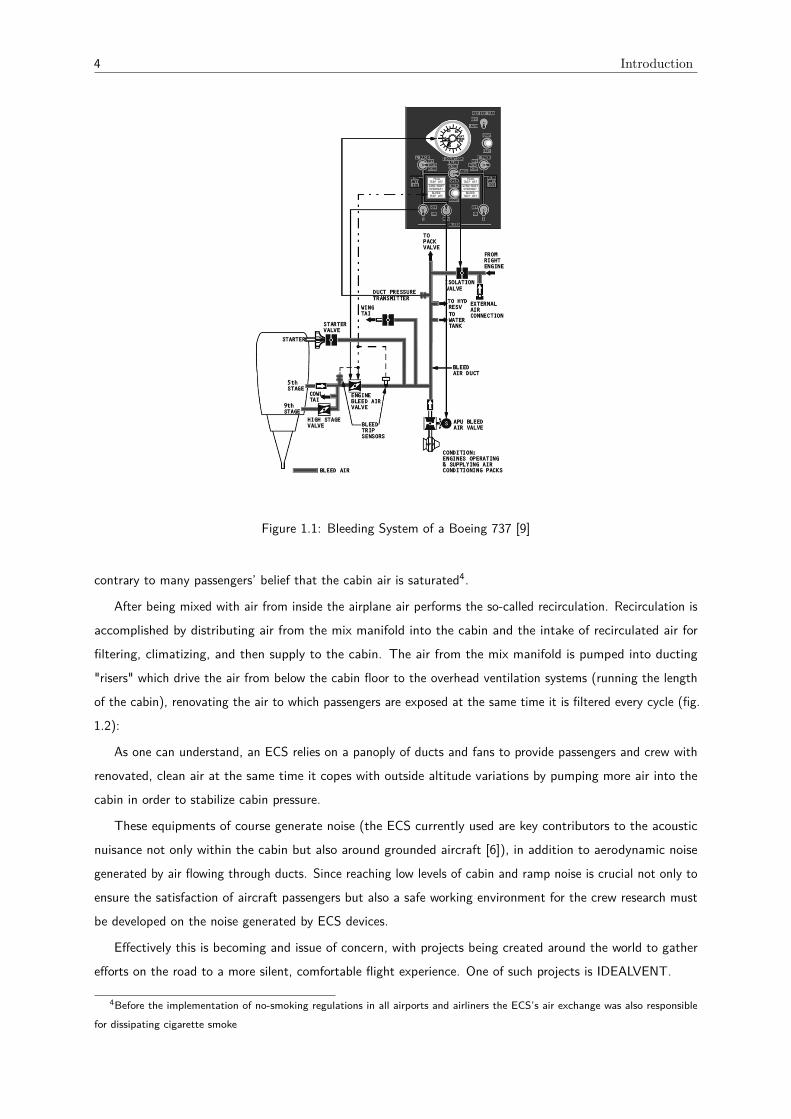
Exits at the engine for pressurized air assigned to the ECS are called bleeding holes. These bleeding holes arelocated at different stages of the compressor, with each stage corresponding to a different value of temperaturein need. After exiting the engine through the bleed hole air is carried into the ECS at high pressure, flowingthrough an intricate duct system (bleeding system, fig. 1.1). The bleeding system is composed of a number ofvalves and a heat exchanger for pre-cooling the air that has been extracted from the engine, since this leavesthe engine at temperatures higher than the desirable. The air extracted by the bleeding system can also beused for potable water pressurization, air-driven hydraulic pumps, and even cargo heat, but of course here we’llbe mainly interested in cabin pressurization, air conditioning, and ventilation.
After the pack valve, seen in fig. 1.1, the air flows into the air conditioning packs.
Air conditioning packs are cycle refrigeration systems that use air passing through and into the airplaneas the refrigerant, and are located under the wing center section. This is done by a combined turbine andcompressor machine , valves for temperature and flow control, and heat exchangers. These devices copewith temperature and humidity variations throughout flight by means of a water separator and a water bagresponsible for the release of undesirable humidity which in turn could freeze.
Air conditioning packs’ objective is therefore to provide air within health and safety requirements forpassengers and crew: dry, at a correct temperature, sterile, and dust free. The amount of air which the ECSpumps into an airliner cabin is enough to renovate the air inside it approximately every two and half minutes,
3On commercial airliners oxygen masks deploy if the so-called "cabin altitute" (atmospheric altitude corresponding to thecabin’s pressure) climbs above 14,000 feet [3]
4 Introduction
Figure 1.1: Bleeding System of a Boeing 737 [9]
contrary to many passengers’ belief that the cabin air is saturated4.
After being mixed with air from inside the airplane air performs the so-called recirculation. Recirculation isaccomplished by distributing air from the mix manifold into the cabin and the intake of recirculated air forfiltering, climatizing, and then supply to the cabin. The air from the mix manifold is pumped into ducting"risers" which drive the air from below the cabin floor to the overhead ventilation systems (running the lengthof the cabin), renovating the air to which passengers are exposed at the same time it is filtered every cycle (fig.1.2):
As one can understand, an ECS relies on a panoply of ducts and fans to provide passengers and crew withrenovated, clean air at the same time it copes with outside altitude variations by pumping more air into thecabin in order to stabilize cabin pressure.
These equipments of course generate noise (the ECS currently used are key contributors to the acousticnuisance not only within the cabin but also around grounded aircraft [6]), in addition to aerodynamic noisegenerated by air flowing through ducts. Since reaching low levels of cabin and ramp noise is crucial not only toensure the satisfaction of aircraft passengers but also a safe working environment for the crew research mustbe developed on the noise generated by ECS devices.
Effectively this is becoming and issue of concern, with projects being created around the world to gatherefforts on the road to a more silent, comfortable flight experience. One of such projects is IDEALVENT.
4Before the implementation of no-smoking regulations in all airports and airliners the ECS’s air exchange was also responsiblefor dissipating cigarette smoke

Cabin Environment and Comfort 5
Figure 1.2: Schematic view of an ECS air recirculation [10]
1.1.3 IDEALVENT
’Unlike aircraft exterior noise, which has received considerable attention in past and currently running research
projects, the noise emitted by confined flows in ECS assemblies involves complex mechanisms that haven’t
been sufficiently investigated to permit the noise reduction wished by passengers and regulators. Acoustic and
hydrodynamic interactions between subcomponents have so far been largely neglected despite being crucial.’
extracted from idealvent.eu
IDEALVENT is a Level 1 Collaborative Project managed by the von Karman Institute for Fluid Dynamics[6].
The project is aimed at achieving the next stepwise reduction of aircraft cabin and ramp noise, which aretwo important objectives of the Work Programme 2012 for aeronautics.
The consortium regroups 10 research institutes, universities and companies, among them:
• VKI - von Karman Institute for Fluid Dynamics, Belgium
• DLR - Deutschland für Luft-und Raumfahrt, Germany
• KTH - Kungliga Tekniska Hoegskolan, Sweden
• KUL - Katholiehe Universiteit Leuven, Belgium
• ECL - Ecole Centrale de Lyon, France
• LMS - LMS International nv, Belgium
• SNT - Odecon Sweden AB, Sweden
• LTS - Liebherr Aerospace toulouse sas, France

6 Introduction
• NTS - New Technologies and services LLC, Russian Federation
• EMB - Embraer S.A
The project’s methodology will include experimental studies in order to provide a deeper understandingof duct acoustics mechanisms and flow generated noise. Combining accurate scale-resolved methods withlow-CPU cost statistical/stochastic methods will then be proposed as an original modelling and design approach.Integrated passive flow and noise control strategies will be explored both experimentally and numerically. Theknowledge gained in the experimental and numerical investigations of the installation effects will allow to deviseand optimize strategies for reducing ECS generated noise.
The first objective of the project is "to obtain a detailed understanding of the mutual interactions betweencomponents found in ECS systems" [6]. The second is to provide modelling guidelines for the simulation ofsuch systems. The third and final objective is directly aimed at the reduction of cockpit/cabin and rampnoise, through the elaboration of system assembly guidelines and the investigation of passive flow and acousticstrategies.
The final aim of the research will be a final test on a full-scale ECS system, where the impact towardsimproved passenger comfort and airport personnel health will be assessed with respect to the objectives of theWork Programme and relevant regulations for commercial aircraft.
With a practical orientation, IDEALVENT "tackles the noise problem at the source" [6], following theviewpoint of the ECS manufacturer and of the integrator.
Given the complexity of an ECS such as those analyzed in Sec. 1.1.2 the consortium has agreed to retainthe following essential elements: the blowing unit (responsible for inducing flow by speeding the air in the duct)and a duct system including bends, vanes and contractions. At VKI research focused on the study of soundwave propagation across ducts when in the presence of ducts and different terminations and how these differfrom the "clean duct" situation (in other words, when no ducted fan is present and the duct termination isadmitted to be anechoic).
The ultimate objective will be, therefore, to know how each one of this elements behaves and how soundwould propagate across a network composed of ducts connecting such different elements and equipment at itsnodes. The overall methodology for such a scientifical approach can be found in Glav and Åbom [11].
In short, ’ [. . . ] ECS noise reduction constituted the leitmotif for an insight into duct acoustics: the study
of acoustic waves’ propagation along walled ducts [. . . ], a mostly common situation regarding ECS, where so
much of the installations comprises exactly of all sorts of ducts’ Aguiar [12].
1.2 Duct Acoustics and The Two-Microphone Method - A Literature
Review
Although acoustics, "the Science of Sound" [13] has been addressed several times in past literature ductacoustics is somewhat harder to trace. Most of the work presented here follows the theoretical background laidby Rienstra and Hirschberg [14]. However, theoretical duct acoustics has been subject to other studies and
Duct Acoustics and The Two-Microphone Method - A Literature Review 7
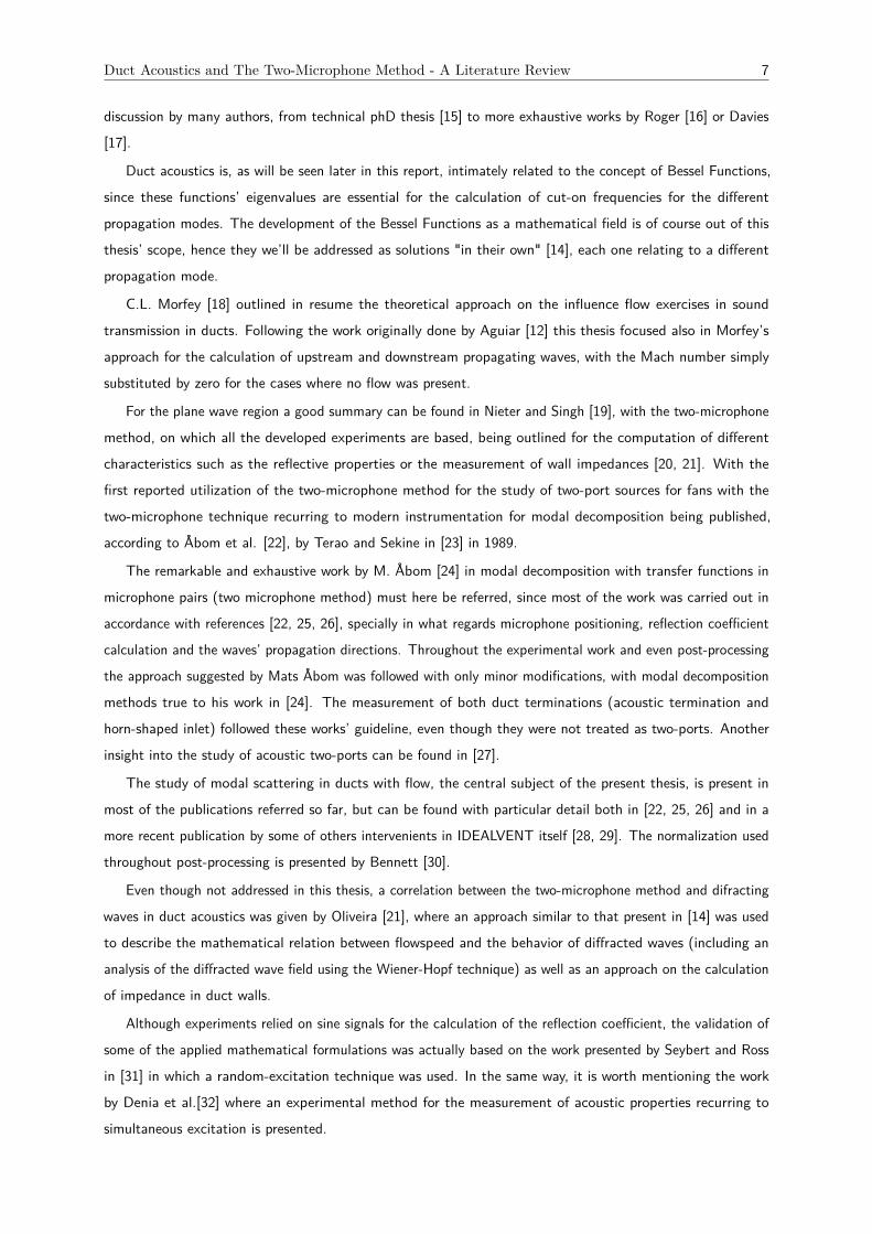
discussion by many authors, from technical phD thesis [15] to more exhaustive works by Roger [16] or Davies[17].
Duct acoustics is, as will be seen later in this report, intimately related to the concept of Bessel Functions,since these functions’ eigenvalues are essential for the calculation of cut-on frequencies for the differentpropagation modes. The development of the Bessel Functions as a mathematical field is of course out of thisthesis’ scope, hence they we’ll be addressed as solutions "in their own" [14], each one relating to a differentpropagation mode.
C.L. Morfey [18] outlined in resume the theoretical approach on the influence flow exercises in soundtransmission in ducts. Following the work originally done by Aguiar [12] this thesis focused also in Morfey’sapproach for the calculation of upstream and downstream propagating waves, with the Mach number simplysubstituted by zero for the cases where no flow was present.
For the plane wave region a good summary can be found in Nieter and Singh [19], with the two-microphonemethod, on which all the developed experiments are based, being outlined for the computation of differentcharacteristics such as the reflective properties or the measurement of wall impedances [20, 21]. With thefirst reported utilization of the two-microphone method for the study of two-port sources for fans with thetwo-microphone technique recurring to modern instrumentation for modal decomposition being published,according to Åbom et al. [22], by Terao and Sekine in [23] in 1989.
The remarkable and exhaustive work by M. Åbom [24] in modal decomposition with transfer functions inmicrophone pairs (two microphone method) must here be referred, since most of the work was carried out inaccordance with references [22, 25, 26], specially in what regards microphone positioning, reflection coefficientcalculation and the waves’ propagation directions. Throughout the experimental work and even post-processingthe approach suggested by Mats Åbom was followed with only minor modifications, with modal decompositionmethods true to his work in [24]. The measurement of both duct terminations (acoustic termination andhorn-shaped inlet) followed these works’ guideline, even though they were not treated as two-ports. Anotherinsight into the study of acoustic two-ports can be found in [27].
The study of modal scattering in ducts with flow, the central subject of the present thesis, is present inmost of the publications referred so far, but can be found with particular detail both in [22, 25, 26] and in amore recent publication by some of others intervenients in IDEALVENT itself [28, 29]. The normalization usedthroughout post-processing is presented by Bennett [30].
Even though not addressed in this thesis, a correlation between the two-microphone method and difractingwaves in duct acoustics was given by Oliveira [21], where an approach similar to that present in [14] was usedto describe the mathematical relation between flowspeed and the behavior of diffracted waves (including ananalysis of the diffracted wave field using the Wiener-Hopf technique) as well as an approach on the calculationof impedance in duct walls.
Although experiments relied on sine signals for the calculation of the reflection coefficient, the validation ofsome of the applied mathematical formulations was actually based on the work presented by Seybert and Rossin [31] in which a random-excitation technique was used. In the same way, it is worth mentioning the workby Denia et al.[32] where an experimental method for the measurement of acoustic properties recurring tosimultaneous excitation is presented.

8 Introduction
Regarding transfer functions, the methodology adopted in this thesis follows the one outlined in otherreferences [22, 25, 26, 33], with the work developed by Chung and Blaser [34, 35] providing both a deepermathematical formulation and references for experimental techniques.
The minimization of errors in measurements effectuated via the two-microphone method has itself alreadybeen subject to several work and investigation. Here the emphasis shall fall upon the analysis performed byBodén and Åbom [36], where a summary description of the method is presented with an input data similar tothat of the present thesis, namely the measured transfer functions, microphone separation, and the distancebetween one microphone and the sample. The analysis of the influence of the different errors (in the transferfunction estimate, in the lengths, and in the calculated quantities) constituted the base for the chapter to comeon this same subject. The effects of flow in ducted flows on acoustical properties was addressed by the sameauthors in [37], and would be adopted in the same way in the present document.
As the option to use over-determination arose other publications had of course to be investigated. Onceagain the work by Mats Åbom and Bodén [38] proved invaluable, with a brief but concise outline of thetechnique. The analysis on error suppression in this thesis follows the one by Bodén et al. [39].
The validation of the codes developed throughout my work was usually effectuated taking an horn-shapedtermination as a reference, since for such kind of acoustic element the reflection coefficient pattern in thefrequency domain is already known and well documented. For this process was essential the study of reflectionin duct terminations by Selamet and Ji in [40] and the analysis presented by Sitel et al. [41]. The similaritiesbetween the inlet used at VKI’s facilities and the horn shaped termination studied by Ville et al. [41] allowedfor a parallelism in analysis and a match in results.
For the analysis of the reflection properties of a discontinuity the work by Akoum and Ville [42] was ofequal great importance, given its remarks on the proper distance to have between both microphones, as well asthe description of test methodologies and result analysis.
The progresses in [41] - when complemented with their discontinuity counterparts in [43] - provided anotherapproach to the same problem, and were eventually followed along with the works presented by Morfey or inreferences [22, 25, 26].
1.3 Aim of the Project
Work currently being developed in VKI in what concerns duct acoustics is intimately related to IDEALVENTand its applications. Since the project was in fact in its beginnings when I started working in Belgium this gaveme the opportunity not only to observe how an international research project is coordinated but also to gain aninsight in duct acoustics and its studies. More work is yet to be made in this field of research, and so thisthesis aims not only to the analysis of a particular experiment (in what would be a so-called case-study) butalso to lay down the basis for any future work concerning modal decomposition in duct acoustics to be carriedout at VKI.
Therefore the mandatory theoretical background will be expanded, including the study of higher ordermodes, and an exhaustive description of experimental methods will be provided. This will include guidelines ontransfer functions, two-microphone methods, and coherence analysis.

Chapter 2
Theoretical Background
To understand the theory behind duct acoustics it is wise to begin with the overall description of the acousticfield. This can be found in the original works by by Rienstra an Hirschberg [14] with impressive depth anddetail, or in a more recent approach by Brambley [44] with equally great accuracy, even if on the expense of anot so straight forward mathematical approach given the non-dimensional variables and different notations inuse. The approach presented in [44] includes in fact a broader perspective, given its scope.
The present thesis focused on the posterior analysis where it was required of the author to find a simplenotation with which to represent the terms in presence and formulate the modal decomposition problem. Thededuction in the present chapter is therefore a synthesis of the one present in [14] for the sake of this thesis’theoretical background.
2.1 Description of the Sound Field
2.1.1 General Formulation
Figure 2.1: Typical duct geometry domain [14]
The problem can be tackled by starting with the basic situation: assuming a duct ∂D to be delimited by atwo dimensional area such as A with boundary ∂A (fig. 2.1) in the same way it was done by Rienstra [14] and
9

10 Theoretical Background
in this author’s previous work (Aguiar [12]), the acoustic field given by (in complex ±iwt sign convention)
p ≡ p(x,w)eiwt, v(x, t) ≡ v(x,w)eiwt (x ∈ D) (2.1)
has been shown both in [14] and [44] to obey the Helmholtz equation and follow a periodic behavior,respectively given by eqs. 2.2a and 2.2b:
∇2p +w2p = 0 (2.2a)
iwv +∇p = 0 (2.2b)
Given the character of this studies it is by far more useful to analyze this problem in the frequency domain.This can be obtained via Fourier synthesis in w and thus the subsequent analysis will always focus on frequencyrather than time domain.
Although the aim of this thesis is in fact an analysis on the experimental methods with which modaldecomposition in duct acoustics is being studied nowadays a synthesized mathematical deduction will be hereperformed for the sake of coherence, following the methodology adopted by Rienstra [14].
It has been shown by the same author [14] that in order to obey the boundary conditions for an enclosedduct surface the following function is obtained:
B (p) = a (y, z) (n ⋅ ∇p) + b (y, z) + c (y, z)∂
∂xp (2.3)
2.3 includes reference to all three coordinates: x, along the duct, and (y, z) in the cross section plane.By assuming the correct boundary conditions as performed by Rienstra it is possible to obtain an equation
for the sound field which obeys the boundary conditions:
B(p) = 0, for x ∈ ∂D (2.4)
The solution to eqs. 2.2a and 2.2b is given considering the appropriate boundary conditions of rigid wall asdone by Rienstra [14] and can be written in the following way [14, 44]:
p(x, y, z) =∞∑n=0
Cnψn(y, z)e−iknx (2.5)
At this point one should take the time to understand what each term in the equation above stands for: Cnis a non-dimensional factor, of which several formulations have been presented and on which we shall developlater; e−iknx deals with the propagation of sound along the duct, with kn referring to the axial wave number.Finally ψn(y, z) describes the variation of acoustic pressure in the section plane. However, all these parcels arein fact, as we can see, part of a general sum of n terms.
The question is, therefore: what is the origin of this n terms, and why has a single equation turned into asum of infinite solutions?
To understand this the reader must know that ψn are in fact “the eigenfunctions of the Laplace operatorreduced to A” [14], solutions of the equations
− (∂2
∂y2 +∂2
∂z2 )ψ = α2ψ for (y, z) ∈ A (2.6a)

Description of the Sound Field 11
B(ψ;α) = 0 for (y, z) ∈ ∂A (2.6b)
One should now regard the similarities between eqs. 2.2a and 2.6a and eqs. 2.2b and 2.6b:
On one hand, eq. 2.2a and 2.6a are in fact similar in the extent that both represent a form of the Helmholtz’swave equation, however, unlike 2.2a, where a general formulation is described which can be applied to thewave as a whole, 2.6a is in fact “attached” to its value for α. In the same way eq. 2.6b follows the sameformulation as its homologous since it represents the same boundary condition although it remains dependenton the considered value of α. If we consider α2 to be the corresponding eigenvalue of the Laplace operatorwhen solving the eq. 2.6a we understand that there is a description of a sound field for every eigenvalue itself.In other words, the description of sound propagation in ducts is actually not given by a unique equation, but bya sum of inner solutions which when added will fully describe the wave’s propagation.
Each one of this solutions is called a mode.
It makes sense then, that, for each mode, we will have another expression for B, which we designed by B.This will this time be given by
B(ψ;α) = a(y, z)(n ⋅ ∇ψ) + b(y, z)ψ − ik(α)c(y, z)ψ (2.7)
The axial wave number can be obtained from the square roots of√
(wc)
2− ( α
R)
2 [14], with each rootrepresenting a different direction for the moving wave (positive and negative roots, left-moving and right-movingwaves).
These eigensolutions consist in fact of combinations of exponentials and Bessel functions [45], with each ofthis combinations representing a mode. In accordance with what is referred in [14] it will only take, as weshall see later on in this thesis, a minor adaptation for this formulation to account for flow effects in soundpropagation in ducts.
The eigenfunctions ψn can be proven to be orthogonal to their complex conjugates ψ∗n by application ofGreen’s Theorem in a the sense that the inner product verifies ([14])
(ψn, ψ∗m) =∬A
ψnψmdσ
⎧⎪⎪⎪⎨⎪⎪⎪⎩
= 0 if n ≠m
≠ 0 if n =m
Which implies that for for real ψn and real αn, as applies to hard-walled ducts where Z is considered to beinfinite, the set of eigenvalues is orthogonal and allows one to calculates modal amplitudes. Given the scopeof this thesis such approach will not be developed, but a deeper analysis can be found in other references[14, 26, 44].
This concludes our first insight into the mathematical basis of modal decomposition: we now have seen thatgiven the imposed boundary conditions in ducts sound transmission cannot be described in a single equation,instead being defined by a sum of modes, each one of them “a solution in itself” [14]. We move therefore, tothe formulation of each one of these modes and how a mathematical approach to modal decomposition can beenvisioned.

12 Theoretical Background
2.1.2 Modal Decomposition in Cylindrical ducts
Before starting the description of sound propagation in cylindrical ducts a note concerning bibliographicalresearch must be here introduced: given different notations and formulations followed by different authorsconsistence between equations and very often unknowns’ symbols it proved difficult to compile all the necessaryinformation making use of only one notation. A more ambitious but fruitful measure was eventually taken,and so from now on the notation used in this report (although closely similar to that used in works by Åbbom[22, 24–26]) is of the author’s own responsibility.
Given the project on which this thesis was developed only cylindrical ducts will be here addressed. For thesame formulations but within rectangular ducts the reader should resort to [14]. For this same reason it wasdecided to use polar coordinates instead of a Cartesian referential. Thus we will define gradient and Laplaceoperator as
∇ = ex∂
∂x+ er
∂
∂r+ ev
1r
∂
∂v(2.8a)
∇2=∂2
∂x2 +∂2
∂r2 +1r
∂
∂r+
1r2
∂2
∂v2 (2.8b)
Which means that the wave equation in 2.2a is now given by
∂2p
∂x2 +∂2p
∂r2 +1r
∂p
∂r+
1r2∂2p
∂v2 +w2p = 0 (2.9)
Now, if we consider a rigid hard-walled wall the impermeability condition must be satisfied and thus we have
∂p
∂r= 0, for r = R (2.10)
where R is the inner radius of the duct in analysis.The solution for the stated problem can be solved via a separation of variables (x, r, and θ), one of many
well documented and explored in a variety of publications. The one presented next was outlined in [14].First we’ll then admit that the pressure p′ at any given point is given by a function in the form
p′ = F (x)G(r)H(θ) (2.11)
And the following conditions must be satisfied [14]:
(d2H
dθ2 ) /H = −m2 (2.12a)
(d2G
dr2 +1r
d2F
dr/G) /G =
m2
r2 − (αmnR
)2
(2.12b)
(d2F
dx2 ) /F = (αmnR
)2− (
w ⋅R
c)
2(2.12c)
In this way the terms relating to each coordinates will be given by
H(θ) = eimθ, m = 0,±1,±2,⋯ (2.13a)
G(r) = Jm(αmnr/R), n = 1,2,⋯ (2.13b)

Description of the Sound Field 13
F (x) = e∓ik±
mnx (2.13c)
Which means that the overall expression for the acoustic field inside the duct will be given by eq. 2.14,whose similarities with eq. 2.5 are easy to understand since it represents the same but this time for polarcoordinates.
p′(x, r, θ) =∞∑
m=−∞
∞∑n=0
(p+m,ne−ik+
m,nx + p−m,ne+ik−
m,nx) fm,n(r)eimθ (2.14)
Where in fact we now have two sums, derived from the necessary separation of variables. At this point oneshould also understand that with this set of equations we can describe the sound field at any given point insidethe duct, since they account for all the coordinates (x,r and θ). By changing these factors and assuming thesum of all modes in presence (later on we will see which modes to consider at different frequencies) we canpredict the acoustic pressure of both moving directions at any position.
Let us then take time to understand what each term exactly represents:
p±m,n represent in fact the acoustic pressure of both directions inside the duct (as seen before, plus and minusamounting to left and right moving, depending on convention). The exponential terms including ±ik+m,nx arerelative to the axial position along the duct with k± being the wave number relative to the waves propagationalong z (the duct’s axis of symmetry) and so designated by axial wave number [26]
kmn =w
c0
√
1 − (α
R
c0
w)
2(2.15)
Where R is the duct’s inner radius as before, c0 the speed of sound, and α is the “nth nonnegative zero ofJ ′m” [14].
The term eimθ regards the point’s azimuthal position in the plane and is associated with m which, byextension, is designated by azimuthal wave number.
Finally fm,n(r) takes in account the point’s position along the duct’s inner radius (i.e. whether it is closeror further away from the plane section’s center) and is given by
fm,n(r) =Jm(αmnr/R)
√Nm,n
(2.16)
One should here realize that fm,n is nothing but the already known function G(r) normalized by√Nm,n.
Throughout the work developed in VKI, and in compliance with other investigation performed in Sweden (see[28, 46]) the function for Nmn in use was the one present in [30], where n represents the radial wave number:
Nmn = J2m (αmn) − Jm−1 (αmn)Jm+1 (αmn) (2.17)
As we can see, what started with basic boundary conditions on the Helmholtz equation (eq. 2.2a) tookus to a superposition of different modes which we can now fully describe for any given point: using threecoordinates associated with the combinations of different wave numbers we are able to outline the acousticfield inside the duct.

14 Theoretical Background
2.1.3 Modes and Cut On Frequencies
The propagation of duct modes is determined by the frequencies in presence. This has already been mentionedin this thesis and will eventually be addressed here:
Let’s begin with the expression describing the sound field inside the duct, whose deduction has alreadybeen here revisioned:
p′(x, r, θ) =∞∑
m=−∞
∞∑n=0
(p+m,ne−ik+
m,nx + p−m,ne+ik−
m,nx) fm,n(r)eimθ (2.18)
The complex notation provides the formulation with the periodic behavior characteristic of an acousticalemission, and if one analyses the exponents it is easy to understand that the only which does not follow thisreasoning is the one concerning the axial coordinate in the term e±ik±m,nx.
Now, if we consider the formulation for the axial wave number kmn given in eq. 2.15:
kmn =w
c0
√
1 − (αmnR
c0
w)
2(2.19)
It comes as a consequence that should the value of kmn be complex its product by i would mean that theaxial term would have a negative exponent:
eik±
m,nx = ei(ai+b)x = e(−a+bi)x = eibxe−ax (2.20)
Here we considered the case of a negative direction, (hence a positive axial wave number), but for theopposite the direction the same applies from symmetry.
Such a mode would then propagate with decreasing amplitude given the term e−ax, which means it wouldbe evanescent, or cut off. In the same way, modes with real kmn will be considered to propagate, and so arecalled cut on.
It is important then, to find the frequencies for which kmn becomes real or complex. Let’s go back toeq. 2.15, but this time taking into account only the expression inside the square root. We know from basicmathematics that kmn will have a complex value when 1 − (
αmnR
c0
w)
2is negative. Therefore we can get the
values of w (and from these, the frequencies) with which kmn acquires either real or complex values:
1 − (αmnR
c0
w)
2= 0 (2.21)
w =αmn ⋅ c0
R(2.22)
Which means that the so called cut on frequencies will be given by:
fcut − onmn =αmn ⋅ c0
2πR(2.23)
Since 2.14 is a sum it means that we can describe the sound field using not the sum of all possible modes,but the sum of all propagating modes, whose kmn is real.
Because “the zeros of J ′m form an ever incrasing sequence both in m and in n [...] there are for any walways an m =m0 and n = n0 beyond which [...] knm is purely imaginary, and the mode decays exponentially
Description of the Sound Field 15
in x”[14]1, it means that for increasing frequencies the value of αmn we will also have to increase for thecut-on condition to be met and so higher order modes will require higher frequencies being emitted.
However, it should be noted that since the first value of αmn (α00) is in fact zero, we will always have√
1 − (αmnR
c0
w)
2= 1, which means that the mode corresponding to α00 will always propagate independently
of the frequency being emitted, even if at higher frequencies kmn is real for other values of αmn and thereforeother modes are not evanescent anymore. This is in fact the plane wave phenomenon, resumed in [12]:
Every signal propagating through a duct induces a plane wave propagation, even if its frequency is higher than
the first cut-on frequency, but requires a frequency higher than the first cut-on frequency for higher modes to
develop.
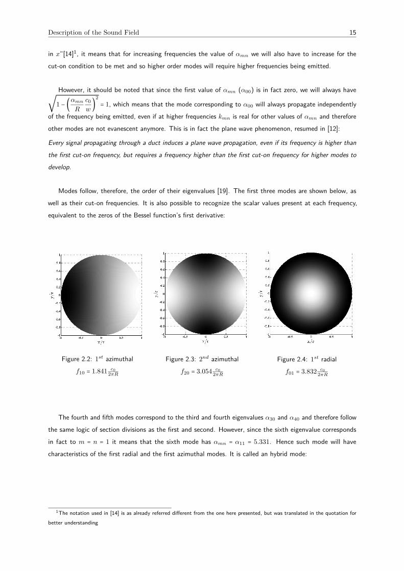
Modes follow, therefore, the order of their eigenvalues [19]. The first three modes are shown below, aswell as their cut-on frequencies. It is also possible to recognize the scalar values present at each frequency,equivalent to the zeros of the Bessel function’s first derivative:
Figure 2.2: 1st azimuthalf10 = 1.841 c0
2πR
Figure 2.3: 2nd azimuthalf20 = 3.054 c0
2πR
Figure 2.4: 1st radialf01 = 3.832 c0
2πR
The fourth and fifth modes correspond to the third and fourth eigenvalues α30 and α40 and therefore followthe same logic of section divisions as the first and second. However, since the sixth eigenvalue correspondsin fact to m = n = 1 it means that the sixth mode has αmn = α11 = 5.331. Hence such mode will havecharacteristics of the first radial and the first azimuthal modes. It is called an hybrid mode:
1The notation used in [14] is as already referred different from the one here presented, but was translated in the quotation forbetter understanding

16 Theoretical Background
Figure 2.5: 1st hybrid f11 = 5.331 c02πR
So far we have considered only the propagation of sound along ducts where no flow is present. This allowedus to describe the sound field along the duct and understand how modes develop at the same time they dependon the frequency emitted. The questions that of course now arise are: how does in-duct flow influence modalpropagation, and how can it be taken into account in the formulations we have gone through in section 2.1?
2.2 Propagation Modes in Cylindrical Ducts with Axial Mean Flow
Although most of the study of sound propagation in ducts with flow actually followed the approach in [18]we will again follow the one in [14] and begin with the linearized equations for small perturbations, where prepresents the acoustic pressure and v the velocity, and M is the flow’s Mach number (Recall eqs. 2.2a and2.2b):
(iw +M∂
∂x)p +∇ ⋅ v = 0 (2.24a)
(iw +M∂
∂x) v +∇ ⋅ p = 0 (2.24b)
A second derivation allows us to eliminate v and obtain the convected wave equation
(iw +M∂
∂x)
2p −∇2p = 0 (2.25)
We can then rewrite eq. 2.25 in the the following form, which comes as familiar after we have solved eq.2.9 in Sec. 2.1.2:
(iw +M∂
∂x)
2p − (
∂2
∂x2 +∂2
∂r2 +1r
∂
∂r+
1r2
∂2
∂θ2 ) = 0 (2.26)
This brings us to the same solution via a separation variables we already found in Sec. 2.1.2:
p′(x, r, θ) =∞∑
m=−∞
∞∑n=0
(p+m,ne−ik+
m,nx + p−m,ne+ik−
m,nx) fm,n(r)eimθ (2.27)
Here we shall recall eqs. 2.28, the first two of which we’ll rewrite in the following way:
Propagation Modes in Cylindrical Ducts with Axial Mean Flow 17
G′′mn +
1rG′mn + (α2
mn −m2
r2 )Gmn = 0(compare with eq. 2.13b) (2.28a)
α2mn = (w −Mkmn)
2− k2
mn (2.28b)
As a consequence, it follows then that the axial wave number will be given by
k±mn =w
c0
√
1 − (αmnR
c0
w)
2(1 −M2) ∓M
1 −M2 (2.29)
The rest of the formulation is in fact identical, and one can see that if we make M = 0 we obtain, asexpected, the no flow situation. This means, then, that the presence of flow does not interfere with modes’shapes, even though it alters cut-on frequencies [12].
The flow speed’s effect on cut-on frequencies can be understood if one analyses eq. 2.29. The term insidethe square root will now be positive or negative depending not only on the signal’s frequency but also on theflow speed in presence. It can be noted then that for a given frequency the presence of flow will in fact shiftaxial wave numbers to the left in the complex plane, if M > 0 or right, should the flow speed be in the oppositedirection (M < 0). To quote Rienstra, “with flow more modes are possibly cut-on” [14]. This will be addressedlater in this thesis.2
2For further reading on this subject the reader should also resort to the work developed in [17, 18]. A deeper numericalformulation for this problem (focused on higher frequencies) can be found in [47], as well as a computation mode-matchingapproach in [48]


Chapter 3
Experimental Methods
The methodology adopted for the acoustic measurements carried out in IDEALVENT is in fact the result ofyears of research and several publications regarding the propagation of sound in duct with and without flow. Itcan be said indeed that the establishment of two-port networks as outlined in [11] will constitute the pinnaclein the study of sound propagation in ducted systems such as those present in aircraft’s ECS or industrialinstallations.
In this chapter, in accordance with what we did for the theoretical basis in presence in this thesis, we’llbegin with the simple basic methodology (the two-microphone method) and after doing so we’ll extrapolate itfor the study of higher order modes in two-port sources, with and without flow.1
Later on in this chapter’s last sections another issue will be addressed, this related to data-acquisition andpost-processing such as coherence, over-determination and transfer functions.
3.1 The Two Microphones Method
The measurement of sound emissions for different mechanical elements such as fans and pumps is of vitalimportance in the study of duct systems and sound propagation across ducts and ducted equipment. A commoncharacteristic to all fluid machines is the presence of both an inlet and an outlet for the fluid to flow. Asreferred in [22] “in the case where one opening is kept unchanged, i.e., the acoustic load seen from this openingnever changes, it can be treated as a part of the source.” This means that the source can be treated as anacoustic one-port source (one can imagine a fan at the end of a duct). This would therefore mean that inthe frequency domain an acoustic one-port can be fully described if we manage to compute its strength andthe reflection at its section. Of course if we consider a two-port (imagine, for example, a ducted fan at aduct’s mid section) then more than reflection only we’ll also also have transmission, thus creating a "two-portacoustic source" problem, since sound not only is emitted and reflected at the outlet and inlet but can also betransmitted across the source itself.
The two-microphone method [49] has been in use for decades in the study of duct acoustics, since itprovides us with a measurement of the acoustic pressure relative to both waves moving in opposite directions
1The study of two-port networks is itself outside the scope of this thesis, hence the reader is encouraged to read [11]
19
20 Experimental Methods
along the duct. The process, based on the solving of the sound field at two given positions inside the ducts,will be outlined in this section.
3.1.1 The Two Microphones Method - One-Port Analysis (Terminations)
The generality of the work conducted in the present section was developed by the author and first demonstratedin [12] mostly based on references [26, 40]. Let’s then begin with the already known expression for the wavepropagation:
p′(x, r, θ) =∞∑
m=−∞
∞∑n=0
(p+m,ne−ik+
m,nx + p−m,ne+ik−
m,nx) fm,n(r)eimθ (3.1)
For now we’ll focus on the plane wave region and therefore exclude from both sums, at the same time wemake m = n = 0.
Later on we’ll see why such a simplification is acceptable, but for now the reader is asked to follow thecurrent approach on the subject. The referred simplification leaves us with
p′(x, r, θ) = (p+0,0e−ik+
0,0x + p−0,0e+ik−
0,0x) f0,0(r)ei0θ (3.2)
Which therefore allows us to rewrite eq.3.2 as
p′(x, r, θ) = (p+e−ik+x+ p−e+ik
−x) f(r) (3.3)
For the sake of a simpler notation we’ll also make p± ∶= p± ⋅ f(r) with makes
p′(x, r, θ) = p+e−ik+x+ p−e+ik
−x (3.4)
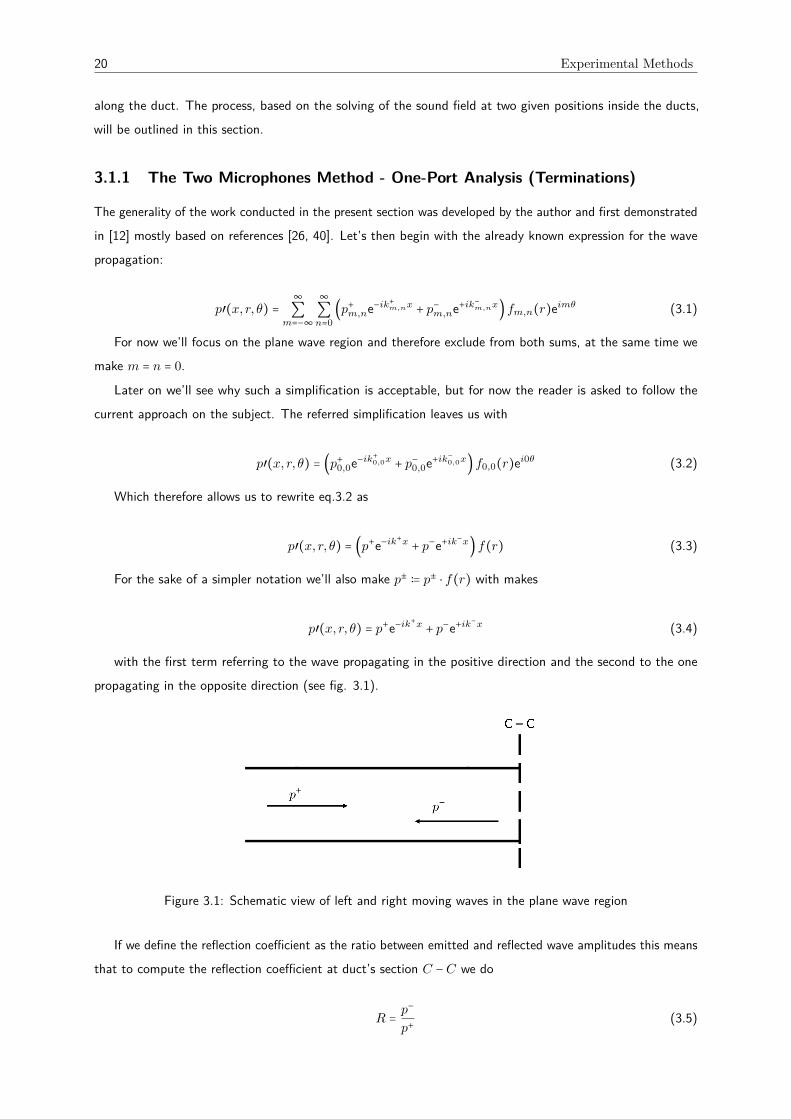
with the first term referring to the wave propagating in the positive direction and the second to the onepropagating in the opposite direction (see fig. 3.1).
Figure 3.1: Schematic view of left and right moving waves in the plane wave region
If we define the reflection coefficient as the ratio between emitted and reflected wave amplitudes this meansthat to compute the reflection coefficient at duct’s section C −C we do
R =p−
p+(3.5)
The Two Microphones Method 21
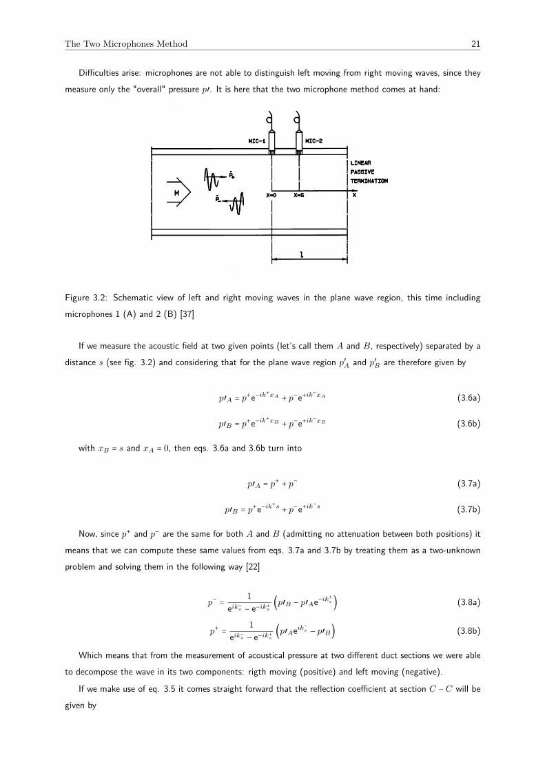
Difficulties arise: microphones are not able to distinguish left moving from right moving waves, since theymeasure only the "overall" pressure p′. It is here that the two microphone method comes at hand:
Figure 3.2: Schematic view of left and right moving waves in the plane wave region, this time includingmicrophones 1 (A) and 2 (B) [37]
If we measure the acoustic field at two given points (let’s call them A and B, respectively) separated by adistance s (see fig. 3.2) and considering that for the plane wave region p′A and p′B are therefore given by
p′A = p+e−ik+xA + p−e+ik
−xA (3.6a)
p′B = p+e−ik+xB + p−e+ik
−xB (3.6b)
with xB = s and xA = 0, then eqs. 3.6a and 3.6b turn into
p′A = p+ + p− (3.7a)
p′B = p+e−ik+s+ p−e+ik
−s (3.7b)
Now, since p+ and p− are the same for both A and B (admitting no attenuation between both positions) itmeans that we can compute these same values from eqs. 3.7a and 3.7b by treating them as a two-unknownproblem and solving them in the following way [22]
p− =1
eik−s − e−ik+s (p′B − p′Ae−ik+
s ) (3.8a)
p+ =1
eik−s − e−ik+s (p′Aeik−
s − p′B) (3.8b)
Which means that from the measurement of acoustical pressure at two different duct sections we were ableto decompose the wave in its two components: rigth moving (positive) and left moving (negative).
If we make use of eq. 3.5 it comes straight forward that the reflection coefficient at section C −C will begiven by

22 Experimental Methods
R =p−
p+=
1eik−s − e−ik+s (p′B − p′Ae−ik
+
s )
1eik−s − e−ik+s (p′Aeik−s − p′B)
=p′B − p′Ae−ik
+
s
p′Aeik−s − p′B(3.9)
This concluding our computation of the plane wave’s reflection coefficient of a termination. Notice we didnot analyze the so-called "active part" since we assumed that no sound is generated at the right of sectionC −C (no source is present, only a strictly reflective section). This of course is purely related to the nature ofthe research developed, where no source was located at the duct’s end, but instead at a mid-section.
In the following section we’ll introduce the study of two-port sources, where we’ll have present not onlythe "passive part" of this section (the capacity of the termination to reflect or transmit sound) but also theacoustic source sound generation and source strength - its "active part".
3.1.2 The Two Microphones Method - Two-Port Analysis
When a coupling between the inlet and outlet is present and conditions on both sides (inlet and outlet) maychange the source must be addressed as a two port, where we can no longer study only one side (inlet oroutlet) and are in fact forced to "duplicate" the analysis performed in section 3.1.1 in order to study both ports.
Much of the work performed on this analysis was based on the works by Åbom [22, 25, 26] and follows thesame approach described by this author. To this contributed of course the fact that in these works the casedescribed is in everything similar to the case studied during my work at VKI and described in the present thesis.
Let’s then consider a configuration similar to that represented in fig. 3.3:
Figure 3.3: Schematic view of a Two-port analysis configuration [22]
The relation between p±a and p±b can be summarized by computing the transmission and reflection coefficientsand adding the source generated acoustic pressure ps. This can be rationalized in the following way: for eachside of the two-port the "outwards moving" wave (identified by a "+" sign) will be given by the sum of thesource generated sound, the transmitted sound from the opposing port, and the reflected sound at the port weare analyzing. For side a this is equivalent to the expression
p+a =
reflection at a³¹¹¹¹¹·¹¹¹¹¹µρa ⋅ p
−a +
transmission across bτb ⋅ p
−b +
source sound at a«ps+a (3.10)
Where ρa represents the reflection coefficient at ports a and b, τa the transmission coefficient across the
The Two Microphones Method 23
two-port source from b to a, and p±a the source generated sound at a moving in the left-to-right direction. Ifwe expand this for the entire two port we get, in the matrix form, for both ports a and b:
⎡⎢⎢⎢⎢⎢⎣
p+a
p+b
⎤⎥⎥⎥⎥⎥⎦
=
⎡⎢⎢⎢⎢⎢⎣
ρa τb
τa ρb
⎤⎥⎥⎥⎥⎥⎦
⎡⎢⎢⎢⎢⎢⎣
p−a
p−b
⎤⎥⎥⎥⎥⎥⎦
+
⎡⎢⎢⎢⎢⎢⎣
ps+a
ps+b
⎤⎥⎥⎥⎥⎥⎦
≡ p+ = Sp− + ps (3.11)
Which allows to conclude that in order to characterize an active two-port S and ps must be determined[22].
However, here we have yet another problem related with the limitations intrinsic to the use of microphones:as referred before when the two-microphone method was being outlined it is not possible for microphonesto distinguish between left and right moving waves (p+ and p−), in the same way it is not possible forthem to identify which part of all the sound they are receiving is in fact emitted by the source (ps) orsimply reflected/transmitted. It is therefore mandatory to divide the two-port source behavior in two distinctcomponents: one associated to its transmission and reflection coefficients, related to how it behaves in thepresent of an external sound source - its passive part; another related corresponding to the noise itself produces,whether it is a fan, a pump, or a valve - its active part.
Two-Port Analysis - Passive Part
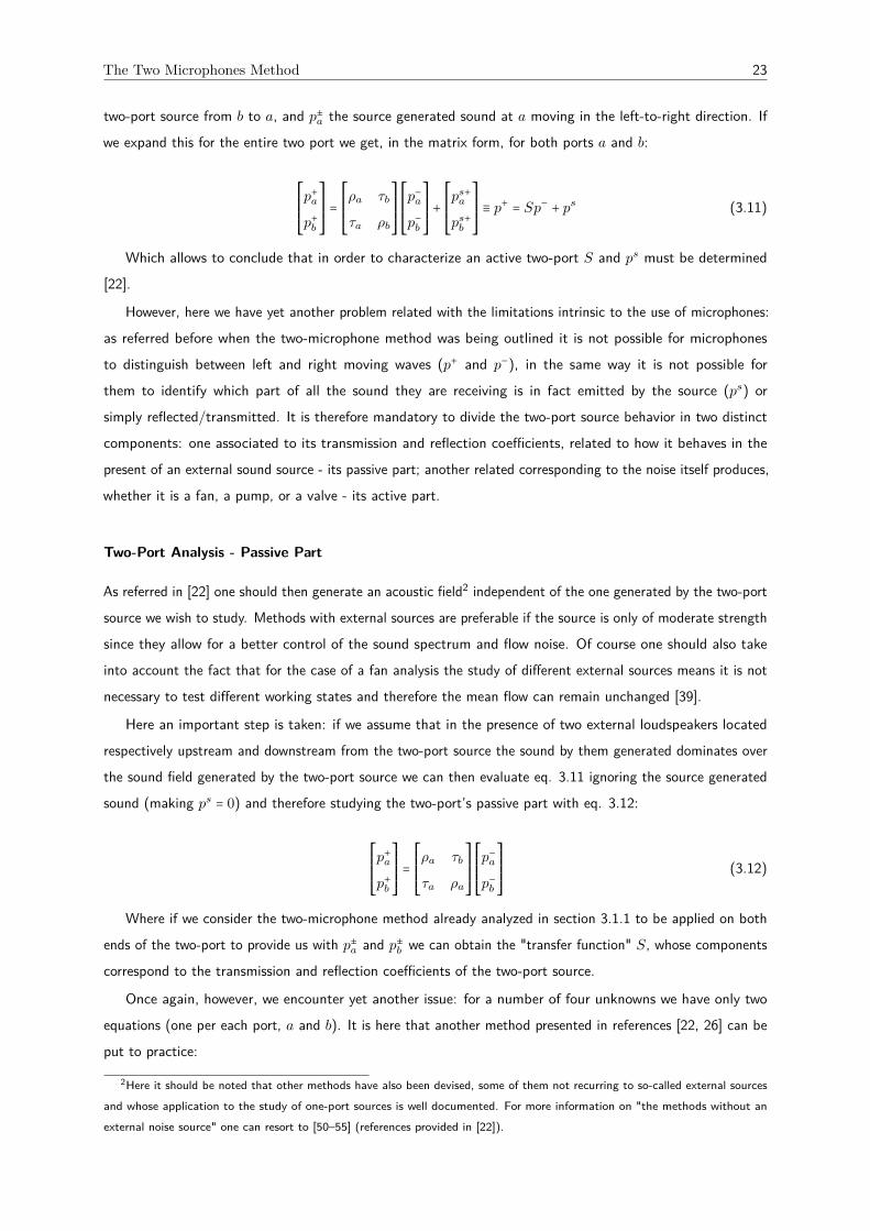
As referred in [22] one should then generate an acoustic field2 independent of the one generated by the two-portsource we wish to study. Methods with external sources are preferable if the source is only of moderate strengthsince they allow for a better control of the sound spectrum and flow noise. Of course one should also takeinto account the fact that for the case of a fan analysis the study of different external sources means it is notnecessary to test different working states and therefore the mean flow can remain unchanged [39].
Here an important step is taken: if we assume that in the presence of two external loudspeakers locatedrespectively upstream and downstream from the two-port source the sound by them generated dominates overthe sound field generated by the two-port source we can then evaluate eq. 3.11 ignoring the source generatedsound (making ps = 0) and therefore studying the two-port’s passive part with eq. 3.12:
⎡⎢⎢⎢⎢⎢⎣
p+a
p+b
⎤⎥⎥⎥⎥⎥⎦
=
⎡⎢⎢⎢⎢⎢⎣
ρa τb
τa ρa
⎤⎥⎥⎥⎥⎥⎦
⎡⎢⎢⎢⎢⎢⎣
p−a
p−b
⎤⎥⎥⎥⎥⎥⎦
(3.12)
Where if we consider the two-microphone method already analyzed in section 3.1.1 to be applied on bothends of the two-port to provide us with p±a and p±b we can obtain the "transfer function" S, whose componentscorrespond to the transmission and reflection coefficients of the two-port source.
Once again, however, we encounter yet another issue: for a number of four unknowns we have only twoequations (one per each port, a and b). It is here that another method presented in references [22, 26] can beput to practice:
2Here it should be noted that other methods have also been devised, some of them not recurring to so-called external sourcesand whose application to the study of one-port sources is well documented. For more information on "the methods without anexternal noise source" one can resort to [50–55] (references provided in [22]).

24 Experimental Methods
By testing the system with two different states (here denoted in roman notation I and II) both upstreamand downstream (that is, with one loudspeaker downstream and another upstream) we will therefore have twomore state equations to solve, since we have expanded both p+ and p− from 2 × 1 vectors to 2 × 2 matrices:
⎡⎢⎢⎢⎢⎢⎣
p+a
p+b
⎤⎥⎥⎥⎥⎥⎦
→
⎡⎢⎢⎢⎢⎢⎣
p+aI
p+aII
p+bI
p+bII
⎤⎥⎥⎥⎥⎥⎦
(3.13a)
⎡⎢⎢⎢⎢⎢⎣
p−a
p−b
⎤⎥⎥⎥⎥⎥⎦
→
⎡⎢⎢⎢⎢⎢⎣
p−aI
p−aII
p−bI
p−bII
⎤⎥⎥⎥⎥⎥⎦
(3.13b)
Which now allows us to easily compute the scattering matrix by doing
S =
⎡⎢⎢⎢⎢⎢⎣
p+aI
p+aII
p+bI
p+bII
⎤⎥⎥⎥⎥⎥⎦
⋅
⎡⎢⎢⎢⎢⎢⎣
p−aI
p−aII
p−bI
p−bII
⎤⎥⎥⎥⎥⎥⎦
−1
(3.14)
Thus concluding the analysis of the passive port for the two-port source.
Two-Port Analysis - Active Part
After computing the scattering matrix of the two-port source the next logical step is therefore to compute ps
which represents, as referred before, the sound generated by the two-port source while working. Be it a fan, apump, or any other ECS component.
Let’s go back to eq. 3.11 for the sake of continuity:
p+ = Sp− + ps (3.15)
Although it can be taken straightforwardly that the source generated acoustic pressure is given by ps =p+ − Sp− it is wise to follow the procedure detailed in [22] and represent ps in order to the acoustic pressuresmeasured at a and b by doing ps = Cp, where p is a vector composed of the acoustic pressures registered ateach first microphone on each side of the two-port and C is in fact a function of the scattering matrix:
⎡⎢⎢⎢⎢⎢⎣
ps+a
ps+b
⎤⎥⎥⎥⎥⎥⎦
= [C]
⎡⎢⎢⎢⎢⎢⎣
pa1
pb1
⎤⎥⎥⎥⎥⎥⎦
(3.16)
Where C is in fact nothing but the simplification of the passive-part process and the solving of eq.3.15 [22]:
C = (I − SR) (I +R)−1 (3.17)
With I being the identity matrix and R the reflection matrix of the two-port sides. At first the computationof R may seem tricky, since it can easily be mistaken by matrices ρa/b. Here one should stop and take time tounderstand what is actually the difference between Ra/b and ρa/b: whereas ρa/b represents the reflection at thetwo-port side Ra/b refers to the reflection at the microphone section, obtained by measuring the sound fieldat a1 and b1 and given by the very same procedure that allowed us to compute the reflection coefficient onsection 3.1.1 (3.18). This may seem somewhat confusing but we must not ignore that reflection may also occurdownstream from the microphone rig or at the microphone rig itself, thus meaning that some of sound arriving
Expanding The Two Microphones Method 25
at the two-port may be in fact sound emitted by the source and reflected at a some downstream location inthe duct. In a word: if the reflection at the two-port source is given by p+/p−, the reflection at the microphoneis therefore given by p−/p+.
R =
⎡⎢⎢⎢⎢⎢⎣
Ra 0
0 Rb
⎤⎥⎥⎥⎥⎥⎦
, with Ra = p−a/pa + and Rb = p−b /pb+ (3.18)
From eq. 3.16 we therefore take the source generated acoustic pressure, thus concluding the active partanalysis.
3.2 Expanding The Two Microphones Method
A reader with a good memory may remember how in section 3.1.1 we started our deduction by constrainingourselves to the plane wave region. At the moment this seemed appropriate since we were introducing amethodology which had not been approached yet hence the decision to keep things as simple as possible at thetime. However this thesis concerns of modal decomposition, and so a method to analyze higher order modesmust come to hand.
Let’s then return to eq. 3.1:
p′(x, r, θ) =∞∑
m=−∞
∞∑n=0
(p+m,ne−ik+
m,nx + p−m,ne+ik−
m,nx) fm,n(r)eimθ (3.19)
It is noted that by suppressing the terms concerning the radial position r and azimuthal coordination θ wewere able to decompose sound propagation in left and right moving by measuring acoustic pressure at twodifferent positions (so-called two-microphone method).
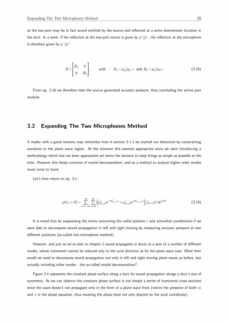
However, and just as we’ve seen in chapter 2 sound propagates in ducts as a sum of a number of differentmodes, whose movement cannot be reduced only to the axial direction as for the plane wave case. What thenwould we need to decompose sound propagation not only in left and right moving plane waves as before, butactually including other modes - the so-called modal decomposition?
Figure 3.4 represents the constant phase surface along a duct for sound propagation alongs a duct’s axis ofsymmetry. As we can observe the constant phase surface is not simply a series of transverse cross sectionssince the wave doesn’t not propagate only in the form of a plane wave front (notice the presence of both mand x in the phase equation, thus meaning the phase does not only depend on the axial coordinate).

26 Experimental Methods
Figure 3.4: Line of constant phase mθ + Re (kmn)x
Since the propagating modes are different from the plane wave it means that acoustic pressure will notbe constant along a duct’s transverse section. In other words, it will depend on both azimuthal and radialpositions within the sound field.
One can then, in compliance with what has been just said, expand the reasoning we followed for theplane-wave region to other wave modes [33]: the same way for the plane wave study we were required tomeasure acoustic pressure at more than one axial coordinate to evaluate wave propagation, we’ll have tomeasure the sound field at more than one azimuthal (and radial, although radial modes were not analyzed inthis project) in order to describe sound variation within a duct transverse section (see fig. 3.5).
Figure 3.5: Schematic view of an expanded analysis microphone set. The azimuthal coordinates of each of themicrophones will be addressed later on in this thesis
This takes us to what we will here describe by "Expanded Analysis", the analysis based on modaldecomposition for other modes than the plane wave, on which will consist the basis for sections 3.2.1 and 3.2.2.
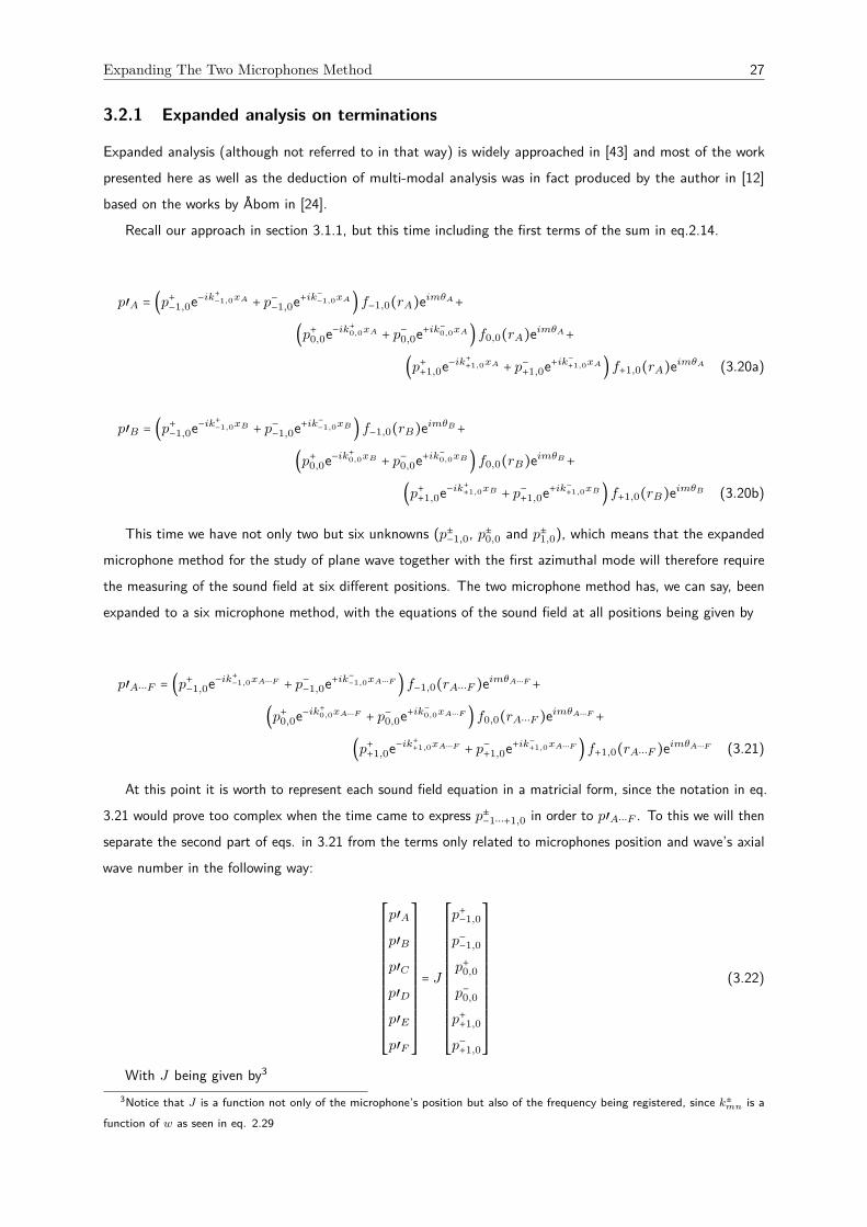
Expanding The Two Microphones Method 27
3.2.1 Expanded analysis on terminations
Expanded analysis (although not referred to in that way) is widely approached in [43] and most of the workpresented here as well as the deduction of multi-modal analysis was in fact produced by the author in [12]based on the works by Åbom in [24].
Recall our approach in section 3.1.1, but this time including the first terms of the sum in eq.2.14.
p′A = (p+−1,0e−ik+
−1,0xA + p−−1,0e+ik−
−1,0xA) f−1,0(rA)eimθA+
(p+0,0e−ik+
0,0xA + p−0,0e+ik−
0,0xA) f0,0(rA)eimθA+
(p++1,0e−ik+
+1,0xA + p−+1,0e+ik−
+1,0xA) f+1,0(rA)eimθA (3.20a)
p′B = (p+−1,0e−ik+
−1,0xB + p−−1,0e+ik−
−1,0xB) f−1,0(rB)eimθB+
(p+0,0e−ik+
0,0xB + p−0,0e+ik−
0,0xB) f0,0(rB)eimθB+
(p++1,0e−ik+
+1,0xB + p−+1,0e+ik−
+1,0xB) f+1,0(rB)eimθB (3.20b)
This time we have not only two but six unknowns (p±−1,0, p±0,0 and p±1,0), which means that the expandedmicrophone method for the study of plane wave together with the first azimuthal mode will therefore requirethe measuring of the sound field at six different positions. The two microphone method has, we can say, beenexpanded to a six microphone method, with the equations of the sound field at all positions being given by
p′A⋯F = (p+−1,0e−ik+
−1,0xA⋯F + p−−1,0e+ik−
−1,0xA⋯F ) f−1,0(rA⋯F )eimθA⋯F +
(p+0,0e−ik+
0,0xA⋯F + p−0,0e+ik−
0,0xA⋯F ) f0,0(rA⋯F )eimθA⋯F +
(p++1,0e−ik+
+1,0xA⋯F + p−+1,0e+ik−
+1,0xA⋯F ) f+1,0(rA⋯F )eimθA⋯F (3.21)
At this point it is worth to represent each sound field equation in a matricial form, since the notation in eq.3.21 would prove too complex when the time came to express p±−1⋯+1,0 in order to p′A⋯F . To this we will thenseparate the second part of eqs. in 3.21 from the terms only related to microphones position and wave’s axialwave number in the following way:
⎡⎢⎢⎢⎢⎢⎢⎢⎢⎢⎢⎢⎢⎢⎢⎢⎢⎢⎢⎣
p′A
p′B
p′C
p′D
p′E
p′F
⎤⎥⎥⎥⎥⎥⎥⎥⎥⎥⎥⎥⎥⎥⎥⎥⎥⎥⎥⎦
= J
⎡⎢⎢⎢⎢⎢⎢⎢⎢⎢⎢⎢⎢⎢⎢⎢⎢⎢⎢⎣
p+−1,0
p−−1,0
p+0,0
p−0,0
p++1,0
p−+1,0
⎤⎥⎥⎥⎥⎥⎥⎥⎥⎥⎥⎥⎥⎥⎥⎥⎥⎥⎥⎦
(3.22)
With J being given by3
3Notice that J is a function not only of the microphone’s position but also of the frequency being registered, since k±mn is afunction of w as seen in eq. 2.29

28 Experimental Methods
J =
⎡⎢⎢⎢⎢⎢⎢⎢⎢⎢⎢⎢⎢⎢⎢⎢⎢⎢⎢⎣
e−ik+−N,0xAf−N,0(rA)eiNθA e+ik−−N,0xAf−N,0(rA)eiNθA ⋯ ⋯ e−ik+N,0xAfN,0(rA)eiNθA e+ik−N,0xAfN,0(rA)eiNθA
⋮ ⋮ ⋯ ⋯ ⋮ ⋮
⋮ ⋮ ⋯ ⋯ ⋮ ⋮
⋮ ⋮ ⋯ ⋯ ⋮ ⋮
⋮ ⋮ ⋯ ⋯ ⋮ ⋮
e−ik+−N,0xF f−N,0(rF )eiNθF e+ik−−N,0xF f−N,0(rF )eiNθF ⋯ ⋯ e−ik+N,0xF fN,0(rF )eiNθF e+ik−N,0xF fN,0(rF )eiNθF
⎤⎥⎥⎥⎥⎥⎥⎥⎥⎥⎥⎥⎥⎥⎥⎥⎥⎥⎥⎦
(3.23)
From here we pass on to the following task of computing the reflection coefficients at the terminationin analysis. Notice we can no longer speak of “a reflection coefficient” since now we have more modes inpresence, each one with its own reflection coefficient, and, as we’ll later see, interacting with other modes.
Recall eq. 3.5. If we defined the reflection coefficient as the ratio between the amplitudes of both emittedand reflected waves we would simply have to divide p−−1,0 by p+−1,0 for the calculation of the reflection coefficientof the first negative azimuthal mode and compute the other reflection coefficients in the same way. However, ashas been demonstrated in [25] and summarized in [12] that computation cannot be performed since althougheach one of these modes is a “solution in itself” [14] it does not propagate alone, rather in addition to all theother previous cut on (notice that equation 2.14 is a sum, rather than a set of equations for each differentmode).
This said, we’ll analyze the reflection mechanism in the following way, as done in [12]:
[R] = [p−] ⋅ [p+]−1 (3.24)
Where p− and p+ are column vectors whose components are the left and right moving modal waves, as
p+ =
⎡⎢⎢⎢⎢⎢⎢⎢⎢⎣
p+−1,0
p+0,0
p++1,0
⎤⎥⎥⎥⎥⎥⎥⎥⎥⎦
; p− =
⎡⎢⎢⎢⎢⎢⎢⎢⎢⎣
p−−1,0
p−0,0
p−+1,0
⎤⎥⎥⎥⎥⎥⎥⎥⎥⎦
(3.25)
While for a more general case we would have4
p+ =
⎡⎢⎢⎢⎢⎢⎢⎢⎢⎣
p+−N,0⋮
p++N,0
⎤⎥⎥⎥⎥⎥⎥⎥⎥⎦
; p− =
⎡⎢⎢⎢⎢⎢⎢⎢⎢⎣
p−−N,0⋮
p−+N,0
⎤⎥⎥⎥⎥⎥⎥⎥⎥⎦
(3.26)
Here we are again faced with an algebric issue: a column vector (2N + 1 × 1) cannot be inverted, thusmeaning that R cannot be directly computed from eq. 3.24 without introducing the same mathematical schemeused in Sec. 3.1.2 (eqs. 3.13 and 3.49). Which means it is necessary to expand 3.26 via a set of 2N + 1 testsituations to obtain square matrices as shown below.
4Notice that now we are only considering the cases with n = 0. This issue will be properly addressed later.

Expanding The Two Microphones Method 29
p+ =
⎡⎢⎢⎢⎢⎢⎢⎢⎢⎣
p+−1,0I
p+−1,0II
p+−1,0III
p+0,0I
p+0,0II
p+0,0III
p++1,0I
p++1,0II
p++1,0III
⎤⎥⎥⎥⎥⎥⎥⎥⎥⎦
; p− =
⎡⎢⎢⎢⎢⎢⎢⎢⎢⎣
p−−1,0I
p−−1,0II
p−−1,0III
p−0,0I
p−0,0II
p−0,0III
p−+1,0I
p−+1,0II
p−+1,0III
⎤⎥⎥⎥⎥⎥⎥⎥⎥⎦
(3.27)
With the general formulation being therefore given by
p+ =
⎡⎢⎢⎢⎢⎢⎢⎢⎢⎣
p+−N,0I
⋯ ⋯ p+−N,02N+1
⋮ ⋯ ⋯ ⋮
p++N,0I
⋯ ⋯ p++N,02N+1
⎤⎥⎥⎥⎥⎥⎥⎥⎥⎦
; p− =
⎡⎢⎢⎢⎢⎢⎢⎢⎢⎣
p−−N,0I
⋯ ⋯ p−−N,02N+1
⋮ ⋯ ⋯ ⋮
p−+N,0I
⋯ ⋯ p−+N,02N+1
⎤⎥⎥⎥⎥⎥⎥⎥⎥⎦
(3.28)
This methodology, extensively developed in [26] proceeds on the the computation of the reflection matrix,given in consequence by
R = [p−] ⋅ [p+]−1=
⎡⎢⎢⎢⎢⎢⎢⎢⎢⎣
p−−N,0I
⋯ ⋯ p−−N,02N+1
⋮ ⋯ ⋯ ⋮
p−+N,0I
⋯ ⋯ p−+N,02N+1
⎤⎥⎥⎥⎥⎥⎥⎥⎥⎦
⋅
⎡⎢⎢⎢⎢⎢⎢⎢⎢⎣
p+−N,0I
⋯ ⋯ p+−N,02N+1
⋮ ⋯ ⋯ ⋮
p++N,0I
⋯ ⋯ p++N,02N+1
⎤⎥⎥⎥⎥⎥⎥⎥⎥⎦
−1
(3.29)
The analysis of each of this matrix’s component’s meaning is provided by the author in [12], with specialrelevance being given to the case of an up-to-first-azimuthal-mode analysis, and will here be addressed followingthe same methodology.
In order to understand the physical meaning of R’s components we can begin by writing the expression forone of the components in p− in order to both R’s coefficients and p+’s (M represents the reference to theexternal source in action).
p−m0M
= p+−N,0M⋅Rm,1 + p
+−N+1,0
M⋅Rm,2 +⋯ + p++N,0
M⋅Rm,2N+1 (3.30)
5It is then definitely worthy to carefully analyze a particular case, in order to realize that another phenomenonarises from the computation of R: modal coupling or modal interaction. With this in mind let’s then writedown the expression for p−−1,0
I for the case of an up-to-first-azimuthal-mode analysis:
p−−1,0I= p+−1,0
I⋅R11 + p
+0,0
I⋅R12 + p
++1,0
I⋅R13 (3.31)
From looking at terms R11 R12 R13 one can think of them as the weight values for the scatter effect ofa given mode on the reflection of the others. In this sense R11 can therefore be understood as the Direct
Reflection Coefficient [12] for the first azimuhtal mode in the negative direction (m = −1), in the same wayR12 quantifies the coupling of the plane wave (m = 0) with the first azimuthal.
In order words, R11 gives us a measure of the portion of the negative first azimuthal to be reflected asitself, at the same time R12 and R13 provide the ration of reflection as plane wave or its opposite, the positivefirst azimuthal mode.6
5Caution is here necessary when addressing the terms from R matrix: although we have written Rm,2N+1 this is in fact a"linguistic liberty" so to speak, since there could not be of course terms with negative indexes for m < 0. What we mean byRm,2N+1 is in fact that each line is assigned to a different azimuthal mode, with the first being related to m = −N and the last tom = +N . The reader is, at this point, advised to write down the expression for better understanding of the algebraic formulation.
6Some authors refer to such coefficients as “conversion coefficients”.
30 Experimental Methods
The general form of a reflection matrix will be as shown, with N being the total number of modes analysed,including the plane wave it self, which will always occupy the middle row [12]:
R =
⎡⎢⎢⎢⎢⎢⎢⎢⎢⎢⎢⎢⎢⎢⎢⎢⎣
R−N,−N ⋯ ⋯ ⋯ R−N,N
⋮ ⋱ ⋯ ⋯ ⋮
R0,−N ⋯ R0,0 ⋯ R0,N
⋮ ⋯ ⋯ ⋱ ⋮
RN,−N ⋯ ⋯ ⋯ RN,N
⎤⎥⎥⎥⎥⎥⎥⎥⎥⎥⎥⎥⎥⎥⎥⎥⎦
(3.32)
Non-coupled modes and Reflection Matrices’ Patterns - The axissymmetric duct
Now that we possess the complete formulation for the study modal decomposition prior to the appearanceof hybrid modes7 we can therefore take time to actually address the constitution of this same matrices wehave deduced. For the sake of simplicity, and without loss of generality let’s choose as an example a reflectionmatrix built including only the plane wave and first azimuthal mode (3 × 3):
R =
⎡⎢⎢⎢⎢⎢⎢⎢⎢⎣
R11 R12 R13
R21 R22 R23
R31 R32 R33
⎤⎥⎥⎥⎥⎥⎥⎥⎥⎦
(3.33)
It is legitimate to question what effect zeros will have in the reflective behavior of the termination in analysis.Let R be
R =
⎡⎢⎢⎢⎢⎢⎢⎢⎢⎣
R11 R12 R13
0 R22 R23
0 R32 R33
⎤⎥⎥⎥⎥⎥⎥⎥⎥⎦
(3.34)
It comes straightforward that the scatter of both plane-wave and first positive azimuthal wouldn’t becoupled with the negative first azimuthal mode. Therefore for a diagonal reflection matrix no coupling at allshould appear, thus meaning the reflection source to be somewhat singular: no mode interacts with any other,reflecting only itself without degenerating into different orders. For this special case, whose matrix is as follows:
R =
⎡⎢⎢⎢⎢⎢⎢⎢⎢⎣
R−N,N 0
⋱
0 RN,N
⎤⎥⎥⎥⎥⎥⎥⎥⎥⎦
(3.35)
Reflection coefficients actually simplify (assuming n = 0) into Rm0 =p−m0p+m0
. This theoretical supposition, also referred by Sitel et al. in [41], would then correspond to the expected result to be obtained from theanalysis of a purely axi-symetric environment where “no conversion between azimuthal modes can occur” [41].This will later be evaluated and constitutes one of the main theoretical assumptions to take in account duringour results’ analysis.
7Although beyond the scope of this thesis (such modes were not addressed during experimental work) a brief section of thiswork will later address possible a possible notation for the study of radial modes.
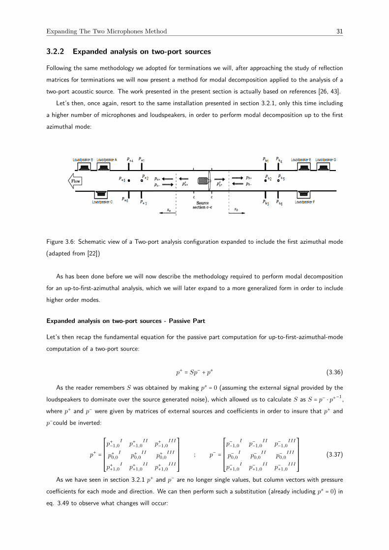
Expanding The Two Microphones Method 31
3.2.2 Expanded analysis on two-port sources
Following the same methodology we adopted for terminations we will, after approaching the study of reflectionmatrices for terminations we will now present a method for modal decomposition applied to the analysis of atwo-port acoustic source. The work presented in the present section is actually based on references [26, 43].
Let’s then, once again, resort to the same installation presented in section 3.2.1, only this time includinga higher number of microphones and loudspeakers, in order to perform modal decomposition up to the firstazimuthal mode:
Figure 3.6: Schematic view of a Two-port analysis configuration expanded to include the first azimuthal mode(adapted from [22])
As has been done before we will now describe the methodology required to perform modal decompositionfor an up-to-first-azimuthal analysis, which we will later expand to a more generalized form in order to includehigher order modes.
Expanded analysis on two-port sources - Passive Part
Let’s then recap the fundamental equation for the passive part computation for up-to-first-azimuthal-modecomputation of a two-port source:
p+ = Sp− + ps (3.36)
As the reader remembers S was obtained by making ps = 0 (assuming the external signal provided by theloudspeakers to dominate over the source generated noise), which allowed us to calculate S as S = p− ⋅ p+−1,where p+ and p− were given by matrices of external sources and coefficients in order to insure that p+ andp−could be inverted:
p+ =
⎡⎢⎢⎢⎢⎢⎢⎢⎢⎣
p+−1,0I
p+−1,0II
p+−1,0III
p+0,0I
p+0,0II
p+0,0III
p++1,0I
p++1,0II
p++1,0III
⎤⎥⎥⎥⎥⎥⎥⎥⎥⎦
; p− =
⎡⎢⎢⎢⎢⎢⎢⎢⎢⎣
p−−1,0I
p−−1,0II
p−−1,0III
p−0,0I
p−0,0II
p−0,0III
p−+1,0I
p−+1,0II
p−+1,0III
⎤⎥⎥⎥⎥⎥⎥⎥⎥⎦
(3.37)
As we have seen in section 3.2.1 p+ and p− are no longer single values, but column vectors with pressurecoefficients for each mode and direction. We can then perform such a substitution (already including ps = 0) ineq. 3.49 to observe what changes will occur:

32 Experimental Methods
S =
⎡⎢⎢⎢⎢⎢⎢⎢⎢⎢⎢⎢⎢⎢⎢⎢⎢⎢⎢⎣
⎡⎢⎢⎢⎢⎢⎢⎢⎢⎣
pa−−1,0
I
pa−0,0
I
pa−+1,0
I
⎤⎥⎥⎥⎥⎥⎥⎥⎥⎦
⎡⎢⎢⎢⎢⎢⎢⎢⎢⎣
pa−−1,0
II
pa−0,0
II
pa−+1,0
II
⎤⎥⎥⎥⎥⎥⎥⎥⎥⎦
⎡⎢⎢⎢⎢⎢⎢⎢⎢⎣
pb−−1,0
I
pb−0,0
I
pb−+1,0
I
⎤⎥⎥⎥⎥⎥⎥⎥⎥⎦
⎡⎢⎢⎢⎢⎢⎢⎢⎢⎣
pb−−1,0
II
pb−0,0
II
pb−+1,0
II
⎤⎥⎥⎥⎥⎥⎥⎥⎥⎦
⎤⎥⎥⎥⎥⎥⎥⎥⎥⎥⎥⎥⎥⎥⎥⎥⎥⎥⎥⎦
⋅
⎡⎢⎢⎢⎢⎢⎢⎢⎢⎢⎢⎢⎢⎢⎢⎢⎢⎢⎢⎣
⎡⎢⎢⎢⎢⎢⎢⎢⎢⎣
pa+−1,0
I
pa+0,0
I
pa++1,0
I
⎤⎥⎥⎥⎥⎥⎥⎥⎥⎦
⎡⎢⎢⎢⎢⎢⎢⎢⎢⎣
pa+−1,0
II
pa+0,0
II
pa++1,0
II
⎤⎥⎥⎥⎥⎥⎥⎥⎥⎦
⎡⎢⎢⎢⎢⎢⎢⎢⎢⎣
pb+−1,0
I
pb+0,0
I
pb++1,0
I
⎤⎥⎥⎥⎥⎥⎥⎥⎥⎦
⎡⎢⎢⎢⎢⎢⎢⎢⎢⎣
pb+−1,0
II
pb+0,0
II
pb++1,0
II
⎤⎥⎥⎥⎥⎥⎥⎥⎥⎦
⎤⎥⎥⎥⎥⎥⎥⎥⎥⎥⎥⎥⎥⎥⎥⎥⎥⎥⎥⎦
−1
(3.38)
Both matrices are not square, so cannot be inverted, which means that we are faced with the same problemas in 3.2.1: the number of tests conducted does not allow us to perform the modal decomposition we desire.Notice that in a way all we are doing when performing expanded modal analysis of two-port sources is simplyconducting two one-port expanded analysis on each end of the source in question. Therefore, all it takes tosolve this algebric nuance is to conduct enough tests on each side of the two-port, expanding eqs. 3.39 in thefollowing way.
S =
⎡⎢⎢⎢⎢⎢⎢⎢⎢⎢⎢⎢⎢⎢⎢⎢⎢⎢⎢⎣
pa+−1,0
I⋯ ⋯ ⋯ ⋯ pa
+−1,0
V I
pa+0,0
I⋯ ⋯ ⋯ ⋯ pa
+0,0
V I
pa++1,0
I⋯ ⋯ ⋯ ⋯ pa
++1,0
V I
pb+−1,0
I⋯ ⋯ ⋯ ⋯ pb
+−1,0
V I
pb+0,0
I⋯ ⋯ ⋯ ⋯ pb
+0,0
V I
pb++1,0
I⋯ ⋯ ⋯ ⋯ pb
++1,0
V I
⎤⎥⎥⎥⎥⎥⎥⎥⎥⎥⎥⎥⎥⎥⎥⎥⎥⎥⎥⎦
⋅
⎡⎢⎢⎢⎢⎢⎢⎢⎢⎢⎢⎢⎢⎢⎢⎢⎢⎢⎢⎣
pa−−1,0
I⋯ ⋯ ⋯ ⋯ pa
−−1,0
V I
pa−0,0
I⋯ ⋯ ⋯ ⋯ pa
−0,0
V I
pa−+1,0
I⋯ ⋯ ⋯ ⋯ pa
−+1,0
V I
pb−−1,0
I⋯ ⋯ ⋯ ⋯ pb
−−1,0
V I
pb−0,0
I⋯ ⋯ ⋯ ⋯ pb
−0,0
V I
pb−+1,0
I⋯ ⋯ ⋯ ⋯ pb
−+1,0
V I
⎤⎥⎥⎥⎥⎥⎥⎥⎥⎥⎥⎥⎥⎥⎥⎥⎥⎥⎥⎦
−1
(3.39)
With the transfer matrix S now being given by
S =
⎡⎢⎢⎢⎢⎢⎣
[ρa] [τb]
[τa] [ρb]
⎤⎥⎥⎥⎥⎥⎦
=
⎡⎢⎢⎢⎢⎢⎢⎢⎢⎢⎢⎢⎢⎢⎢⎢⎢⎢⎢⎣
⎡⎢⎢⎢⎢⎢⎢⎢⎢⎣
ρa1,1 ρa1,2 ρa1,3
ρa2,1 ρa2,2 ρa2,3
ρa3,1 ρa3,2 ρa3,3
⎤⎥⎥⎥⎥⎥⎥⎥⎥⎦
⎡⎢⎢⎢⎢⎢⎢⎢⎢⎣
τb1,1 τb1,2 τb1,3
τb2,1 τb2,2 τb2,3
τb3,1 τb3,2 τb3,3
⎤⎥⎥⎥⎥⎥⎥⎥⎥⎦
⎡⎢⎢⎢⎢⎢⎢⎢⎢⎣
τa1,1 τa1,2 τa1,3
τa2,1 τa2,2 τa2,3
τa3,1 τa3,2 τa3,3
⎤⎥⎥⎥⎥⎥⎥⎥⎥⎦
⎡⎢⎢⎢⎢⎢⎢⎢⎢⎣
ρb1,1 ρb1,2 ρb1,3
ρb2,1 ρb2,2 ρb2,3
ρb3,1 ρb3,2 ρb3,3
⎤⎥⎥⎥⎥⎥⎥⎥⎥⎦
⎤⎥⎥⎥⎥⎥⎥⎥⎥⎥⎥⎥⎥⎥⎥⎥⎥⎥⎥⎦
(3.40)
Where the matrices ρa and ρb are the reflection matrices as calculated before for terminations in section3.2.1, whith ρa/b11 ρa/b22 and ρa/b33 constituting the “direct reflection” coefficients and the other terms theso-called conversion coefficients.
In the same logic both matrices τa and τb describe the transmission process across the two-port with somemodes being transmitted as themselves (propagating through the source without suffering scattering) andothers being converted into different propagation modes.
As usual, and following the methodology adopted in this thesis we will conclude this section by outliningthe general forms of both matrices S and p±a/b, for any azimuthal modal decomposition.
As before the relation between the required number of external sources (loudspeakers) tests stands, whichmeans that for an analysis of N azimuthal modes we will need 2N + 1 external sources for matrices to be

Expanding The Two Microphones Method 33
square and thus possible to invert.8 In order words, p+ p− and S will now be given by:
p+ =
⎡⎢⎢⎢⎢⎢⎢⎢⎢⎢⎢⎢⎢⎢⎢⎢⎢⎢⎢⎣
pa+−N,0
I⋯ ⋯ ⋯ ⋯ pa
+−1,0
2N+1
⋮ ⋯ ⋯ ⋯ ⋯ ⋮
pa++N,0
I⋯ ⋯ ⋯ ⋯ pa
++1,0
2N+1
pb+−N,0
I⋯ ⋯ ⋯ ⋯ pb
+−1,0
2N+1
⋮ ⋯ ⋯ ⋯ ⋯ ⋮
pb++N,0
I⋯ ⋯ ⋯ ⋯ pb
++1,0
2N+1
⎤⎥⎥⎥⎥⎥⎥⎥⎥⎥⎥⎥⎥⎥⎥⎥⎥⎥⎥⎦
; p− =
⎡⎢⎢⎢⎢⎢⎢⎢⎢⎢⎢⎢⎢⎢⎢⎢⎢⎢⎢⎣
pa−−N,0
I⋯ ⋯ ⋯ ⋯ pa
−−1,0
2N+1
⋮ ⋯ ⋯ ⋯ ⋯ ⋮
pa−+N,0
I⋯ ⋯ ⋯ ⋯ pa
−+1,0
2N+1
pb−−N,0
I⋯ ⋯ ⋯ ⋯ pb
−−1,0
2N+1
⋮ ⋯ ⋯ ⋯ ⋯ ⋮
pb−+N,0
I⋯ ⋯ ⋯ ⋯ pb
−+1,0
2N+1
⎤⎥⎥⎥⎥⎥⎥⎥⎥⎥⎥⎥⎥⎥⎥⎥⎥⎥⎥⎦
(3.41)
S =
⎡⎢⎢⎢⎢⎢⎢⎢⎢⎢⎢⎢⎢⎢⎢⎢⎢⎢⎢⎣
⎡⎢⎢⎢⎢⎢⎢⎢⎢⎣
ρa1,1 ⋯ ρa1,N
⋮ ⋱ ⋮
ρaN,1 ⋯ ρaN,N
⎤⎥⎥⎥⎥⎥⎥⎥⎥⎦
⎡⎢⎢⎢⎢⎢⎢⎢⎢⎣
τb1,1 ⋯ τb1,N
⋮ ⋱ ⋮
τbN,1 ⋯ τbN,N
⎤⎥⎥⎥⎥⎥⎥⎥⎥⎦
⎡⎢⎢⎢⎢⎢⎢⎢⎢⎣
τa1,1 ⋯ τa1,N
⋮ ⋱ ⋮
τaN,1 ⋯ τaN,N
⎤⎥⎥⎥⎥⎥⎥⎥⎥⎦
⎡⎢⎢⎢⎢⎢⎢⎢⎢⎣
ρb1,1 ⋯ ρb1,N
⋮ ⋱ ⋮
ρbN,1 ⋯ ρbN,N
⎤⎥⎥⎥⎥⎥⎥⎥⎥⎦
⎤⎥⎥⎥⎥⎥⎥⎥⎥⎥⎥⎥⎥⎥⎥⎥⎥⎥⎥⎦
(3.42)
Expanded analysis on two-port sources - Active Part
Calculating the active part of an acoustic two-port source follows the methodology outlined in section 3.2.1 atethe same time it adopts the expanded matrices of the last section.
We can realize the mechanics involved by starting with eq. 3.16, here rewritten for the sake of an easierreasoning:
⎡⎢⎢⎢⎢⎢⎣
ps+a
ps+b
⎤⎥⎥⎥⎥⎥⎦
= [C]
⎡⎢⎢⎢⎢⎢⎣
pa1
pb1
⎤⎥⎥⎥⎥⎥⎦
(3.43)
Notice that as before C is given by
C = (I − SR) (I +R)−1 (3.44)
Now if we consider S already to be now and I once again to be the identity matrix we must refer to R asthe expanded reflection matrix at the microphone section.
This is obtained in the same way as in Sec. 3.2.1 except this time considering not the reflection in thereflection at the two-port (that would, as we have seen before) give us ρa/b but instead at the microphonesection itself, thus being given by R = p− ⋅ p+−1.
From here we obtain for R from the exact same equation we used in section 3.2.1 (eq. 3.29):
R = [p−] ⋅ [p+]−1=
⎡⎢⎢⎢⎢⎢⎢⎢⎢⎣
p−−N,0I
⋯ ⋯ p−−N,02N+1
⋮ ⋯ ⋯ ⋮
p−+N,0I
⋯ ⋯ p−+N,02N+1
⎤⎥⎥⎥⎥⎥⎥⎥⎥⎦
⋅
⎡⎢⎢⎢⎢⎢⎢⎢⎢⎣
p+−N,0I
⋯ ⋯ p+−N,02N+1
⋮ ⋯ ⋯ ⋮
p++N,0I
⋯ ⋯ p++N,02N+1
⎤⎥⎥⎥⎥⎥⎥⎥⎥⎦
−1
(3.45)
8In fact we will observe later that in fact matrices don’t have to 2N + 1 × 2N + 1 square for higher modes to be computed aslong as we include at least 2N + 1 tests. This process is called “over-determination” and will be properly addressed in section 3.3.

34 Experimental Methods
This allows us then to compute C and solve eq. 3.43.
As a final remark one should notice that in the same way we have decomposed the external source generatedsound so far we will also also a (2N + 1) × 1 vector for ps, with each term representing the acoustic pressureemitted in each mode.
3.3 Experimental Over-Determination
So far we have made sure that a matrix could be inverted by testing either enough microphones or externalsources (loudspeakers) for it to happen. However, it has been shown [26, 38] that by assembling measurementsby more than 2N + 1 loudspeakers in each side of a two-port or next to a termination and calculating theso-called “Moore–Penrose pseudoinverse” matrix [56] of either p+ and p− we can in fact suppress the flowinduced noise inside the duct. However it is still required that at least 2N + 1 measurements are linearlyindependent.
Over-determination has not been addressed so far for the sake of simplicity, since it is not a method in itself,rather a modification that can be applied to any modal analysis. Instead it has been decided to present it onlyin the present section, where it will be described how over-determination can be applied to both terminationand two-port analysis.
Much work has been devoted so far to the study of error-suppression via the use of over-determination.Some of the authors being actually related to IDEALVENT. One of such examples can be found in Holmberget. al. [39]. Much of the development in this subject in the present section follows the same approach.
If we think of two-port analysis or even a termination study we realize that most of possible errors comefrom flow induced noise. On cannot, in fact, neglect the turbulence effects in microphones since it induces adisturbance in measurements mostly impossible to predict and difficult to cope with.
It has been sugested by Terao and Sekine [23] that by using two reference microphones low noise couldbe suppressed. This technique was applied for the means of coherence check, since by analyzing coherencewith tow different microphones we were able to spot noise affected frequencies and more important evaluatemicrophones’ performances.9. This process was eventually dismissed since the adopted reference was in factthe source’s signal being emitted by the test’s external source, as suggested by Lavrentjev et. al.[22]. Thismethod would later be used by De Roeck and Desmet to determine the flow noise generated by an expansionchamber, which was described in [57].
3.3.1 Experimental Over-Determination for one-port sources
As referred before over-determination consisted in performing more external source tests than the required. Forthe study of the plane wave reflection coefficient in a termination it consists in rewriting eq. 3.9 as
R = [p−] ⋅ [p−]+ = [p−I ⋯ p−N] ⋅ [p−I ⋯ p+N]+
(3.46)
Where “+” denotes the pseudo-inverse and N is the number of external sources used.9Coherence will later be subject to proper analysis later on in this thesis.
Experimental Over-Determination 35
In a similar faction to include over-determination for expanded analysis of terminations it will only benecessary to perform the same change, this time in eq. 3.29:
R = [p−] ⋅ [p+]−1=
⎡⎢⎢⎢⎢⎢⎢⎢⎢⎣
p−−N,0I
⋯ ⋯ ⋯ p−−N,02N+1
⋮ ⋯ ⋯ ⋯ ⋮
p−+N,0I
⋯ ⋯ ⋯ p−+N,02N+1
⎤⎥⎥⎥⎥⎥⎥⎥⎥⎦
⋅
⎡⎢⎢⎢⎢⎢⎢⎢⎢⎣
p+−N,0I
⋯ ⋯ ⋯ p+−N,02N+1
⋮ ⋯ ⋯ ⋯ ⋮
p++N,0I
⋯ ⋯ ⋯ p++N,02N+1
⎤⎥⎥⎥⎥⎥⎥⎥⎥⎦
+
(3.47)
Moreover, it is possible to expand not only p+ and p− by including more loudspeaker tests, it is also possibleto include more than the required microphones, thus expanding the matrix J itself:
J =
⎡⎢⎢⎢⎢⎢⎢⎢⎢⎢⎢⎢⎢⎢⎢⎢⎢⎢⎢⎣
e−ik+−N,0xAf−N,0(rA)eiNθA e+ik−−N,0xAf−N,0(rA)eiNθA ⋯ ⋯ e−ik+N,0xAfN,0(rA)eiNθA e+ik−N,0xAfN,0(rA)eiNθA
⋮ ⋮ ⋯ ⋯ ⋮ ⋮
⋮ ⋮ ⋯ ⋯ ⋮ ⋮
⋮ ⋮ ⋯ ⋯ ⋮ ⋮
⋮ ⋮ ⋯ ⋯ ⋮ ⋮
e−ik+−N,0xF f−N,0(rF )eiNθF e+ik−−N,0xF f−N,0(rF )eiNθF ⋯ ⋯ e−ik+N,0xF fN,0(rF )eiNθF e+ik−N,0xF fN,0(rF )eiNθF
⎤⎥⎥⎥⎥⎥⎥⎥⎥⎥⎥⎥⎥⎥⎥⎥⎥⎥⎥⎦
(3.48)It has been suggested by Sack [28] that by increasing partial pressure matrices using both more loudspeakers
and microphones the computation of p+ and p− would become more accurate given the suppressing ofexperimental and random errors. This technique would later be implemented throughout test campaigns anddata post-processing.
3.3.2 Experimental Over-Determination for two-port sources
For two-port sources over-determination does not require a problem formerly described by a simple equationto be described in the matricial form as before. In fact for the two-port analysis the only changes requiredfor over-determination to be included consist of writing the p− and p− matrices including more external loads(columns) than before:
S =
⎡⎢⎢⎢⎢⎢⎣
p+aI
⋯ p+aN+NR
p+bI
⋯ p+bN+NR
⎤⎥⎥⎥⎥⎥⎦
⋅
⎡⎢⎢⎢⎢⎢⎣
p−aI
⋯ p−aN+NR
p−bI
⋯ p−bN+NR
⎤⎥⎥⎥⎥⎥⎦
+
(3.49)
Thus expanding eq. 3.39 into
S =
⎡⎢⎢⎢⎢⎢⎢⎢⎢⎢⎢⎢⎢⎢⎢⎢⎢⎢⎢⎣
pa+−1,0
I⋯ ⋯ ⋯ ⋯ ⋯ pa
+−1,0
N
pa+0,0
I⋯ ⋯ ⋯ ⋯ ⋯ pa
+0,0
N
pa++1,0
I⋯ ⋯ ⋯ ⋯ ⋯ pa
++1,0
N
pb+−1,0
I⋯ ⋯ ⋯ ⋯ ⋯ pb
+−1,0
N
pb+0,0
I⋯ ⋯ ⋯ ⋯ ⋯ pb
+0,0
N
pb++1,0
I⋯ ⋯ ⋯ ⋯ ⋯ pb
++1,0
N
⎤⎥⎥⎥⎥⎥⎥⎥⎥⎥⎥⎥⎥⎥⎥⎥⎥⎥⎥⎦
⋅
⎡⎢⎢⎢⎢⎢⎢⎢⎢⎢⎢⎢⎢⎢⎢⎢⎢⎢⎢⎣
pa−−1,0
I⋯ ⋯ ⋯ ⋯ ⋯ pa
−−1,0
N
pa−0,0
I⋯ ⋯ ⋯ ⋯ ⋯ pa
−0,0
N
pa−+1,0
I⋯ ⋯ ⋯ ⋯ ⋯ pa
−+1,0
N
pb−−1,0
I⋯ ⋯ ⋯ ⋯ ⋯ pb
−−1,0
N
pb−0,0
I⋯ ⋯ ⋯ ⋯ ⋯ pb
−0,0
N
pb−+1,0
I⋯ ⋯ ⋯ ⋯ ⋯ pb
−+1,0
V I
⎤⎥⎥⎥⎥⎥⎥⎥⎥⎥⎥⎥⎥⎥⎥⎥⎥⎥⎥⎦
+
(3.50)
It should also be referred that the computation of the active part is not affected since over-determinationdoes not affect the dimensions of S, and, therefore, of C
36 Experimental Methods
3.4 Including Radial Modes
In-duct modal decomposition from 500 to 3500 Hz is only concluded if radial modes are taken into account inthe analysis. The inclusion of such modes had never, to the author’s knowledge, been attempted before, andrepresents the final objective in this work.
In some way the analysis of radial modes is simplistic: if we recall eq. 2.14 it is possible to understand themain aspect of modal decomposition including radial modes: even though the radial component must be takeninto account for every term it doesn’t mean including radial modes will change the equations’ dimensions.
To write down the complete equation for the first radial mode we only have to write all first azimuthalmodes up to the first cut-on (m = ±1 and m = ±2) and include the first radial mode (m = 0, n = 1). As we cansee in eq. 3.52, the sound field will be given, up to the fourth cut-on frequency, by:
p′(x, r, θ) = (p+−2,0e−ik+
−2,0x + p−−2,0e+ik−
−2,0x) f−2,0(r)e−2iθ
+ (p+−1,0e−ik+
−1,0x + p−−1,0e+ik−
−1,0x) f−1,0(r)e−iθ
+ (p+0,0e−ik+
0,0x + p−0,0e+ik−
0,0x) f0,0(r)ei×0×θ
+ (p++1,0e−ik+
+1,0x + p−+1,0e+ik−
+1,0x) f+1,0(r)eiθ
+ (p++2,0e−ik+
+2,0x + p−+2,0e+ik−
+2,0x) f+2,0(r)eiθ
+ (p+0,1e−ik+
0,1x + p−0,1e+ik−
0,1x) f0,1(r)ei×0×θ
´¹¹¹¹¹¹¹¹¹¹¹¹¹¹¹¹¹¹¹¹¹¹¹¹¹¹¹¹¹¹¹¹¹¹¹¹¹¹¹¹¹¹¹¹¹¹¹¹¹¹¹¹¹¹¹¹¹¹¹¹¹¹¹¹¹¹¹¹¹¹¹¹¹¹¹¹¹¹¹¹¹¹¹¹¹¹¹¹¹¹¹¹¹¹¹¹¹¹¹¹¹¹¹¹¹¹¹¹¹¹¹¹¹¹¹¹¹¹¹¹¹¹¹¹¹¹¹¹¹¹¹¹¹¹¸¹¹¹¹¹¹¹¹¹¹¹¹¹¹¹¹¹¹¹¹¹¹¹¹¹¹¹¹¹¹¹¹¹¹¹¹¹¹¹¹¹¹¹¹¹¹¹¹¹¹¹¹¹¹¹¹¹¹¹¹¹¹¹¹¹¹¹¹¹¹¹¹¹¹¹¹¹¹¹¹¹¹¹¹¹¹¹¹¹¹¹¹¹¹¹¹¹¹¹¹¹¹¹¹¹¹¹¹¹¹¹¹¹¹¹¹¹¹¹¹¹¹¹¹¹¹¹¹¹¹¹¹¹¶first radial mode (m = 0, n = 1)
(3.51)
As usual, we will now finish this introduction by laying down what would then be the generalized form forany mode:
p′(x, r, θ) = (p+−2,0e−ik+
−2,0x + p−−2,0e+ik−
−2,0x) f−2,0(r)e−2iθ+⋯
+ (p++2,0e−ik+
+2,0x + p−+2,0e+ik−
+2,0x) f+2,0(r)e+2iθ+⋯
+ (p+0,1e−ik+
0,1x + p−0,1e+ik−
0,1x) f0,1(r)ei×0×θ+⋯
+ (p+m,ne−ik+
m,nx + p−m,ne+ik−
m,nx) fm,n(r)eimθ(3.52)
3.4.1 Radial Modes for terminations
From a measurement point of view the addition of radial modes requires not only more external sources,because since more modes are being taken into account, more linear independent measurements will be requiredin the same way that expanded analysis required more loudspeakers in Sec. 3.2.
For terminations, we will have both p+ and p− expanded to included the radial mode terms, here representedby the last three rows:

Including Radial Modes 37
p+ =
⎡⎢⎢⎢⎢⎢⎢⎢⎢⎢⎢⎢⎢⎢⎢⎢⎢⎢⎢⎣
p+−N,0I
⋯ ⋯ p++N,02N+1+NR
⋮ ⋯ ⋯ ⋮
p+−N,0I
⋯ ⋯ p++N,02N+1+NR
p+0,1I
⋯ ⋯ p+0,12N+1+NR
⋮ ⋯ ⋯ ⋮
p+m,nI
⋯ ⋯ p+m,n2N+1+NR
⎤⎥⎥⎥⎥⎥⎥⎥⎥⎥⎥⎥⎥⎥⎥⎥⎥⎥⎥⎦
; p− =
⎡⎢⎢⎢⎢⎢⎢⎢⎢⎢⎢⎢⎢⎢⎢⎢⎢⎢⎢⎣
p−−N,0I
⋯ ⋯ p−+N,02N+1+NR
⋮ ⋯ ⋯ ⋮
p−−N,0I
⋯ ⋯ p−+N,02N+1+NR
p−0,1I
⋯ ⋯ p−0,12N+1+NR
⋮ ⋯ ⋯ ⋮
p−m,nI
⋯ ⋯ p−m,n2N+1+NR
⎤⎥⎥⎥⎥⎥⎥⎥⎥⎥⎥⎥⎥⎥⎥⎥⎥⎥⎥⎦
(3.53)
Which correspond to the vectors in eqs. 3.28 but this time including the radial modes when such are alsopresent. One should also bear in mind two new aspects of modal decomposition when including radial modes:firstly, since we are now analyzing a higher number of modes more microphones had to be inserted as seenbefore in Sec. 3.2.1, secondly we should also notice how the necessary number of linearly independent test isnow 2N + 1 +NR instead of only 2N + 1. NR is in fact the number of radial modes being analyzed. Noticethat since there are no negative values for n the number of tests is not twice the maximum azimuthal modenumber (discounting the plane wave) as before.
Since the formulation has not changed, but only been expanded, so will be the reflection matrix, representedin the following way in order to take into account the additional radial modes of radial (last two rows):
R =
⎡⎢⎢⎢⎢⎢⎢⎢⎢⎢⎢⎢⎢⎢⎢⎢⎢⎢⎢⎢⎢⎢⎢⎢⎢⎢⎣
R−N,−N ⋯ ⋯ ⋯ R−N,N
⋮ ⋱ ⋯ ⋯ ⋮
R0,−N ⋯ R0,0 ⋯ R0,N
⋮ ⋯ ⋯ ⋱ ⋮
RN,−N ⋯ ⋯ ⋯ RN,N
R0,NR⋯ ⋯ ⋯ RN,N
⋮ ⋯ ⋯ ⋱ ⋮
RN,NR⋯ ⋯ ⋯ RN,N
⎤⎥⎥⎥⎥⎥⎥⎥⎥⎥⎥⎥⎥⎥⎥⎥⎥⎥⎥⎥⎥⎥⎥⎥⎥⎥⎦
(3.54)
3.4.2 Radial Modes for two-port sources
For two-port analysis the method is similar to that of terminations already referred in the previous section.
In the same way we expanded p+ and p− by including the radial modes as extra lines for termination analysisfor two-port analysis.
This means therefore that S (eq. 3.41) is rewritten as
S =
⎡⎢⎢⎢⎢⎢⎢⎢⎢⎢⎢⎢⎢⎢⎢⎢⎢⎢⎢⎣
pa+−1,0
I⋯ ⋯ ⋯ ⋯ ⋯ pa
+−1,0
N
pa+0,0
I⋯ ⋯ ⋯ ⋯ ⋯ pa
+0,0
N
pa++1,0
I⋯ ⋯ ⋯ ⋯ ⋯ pa
++1,0
N
pb+−1,0
I⋯ ⋯ ⋯ ⋯ ⋯ pb
+−1,0
N
pb+0,0
I⋯ ⋯ ⋯ ⋯ ⋯ pb
+0,0
N
pb++1,0
I⋯ ⋯ ⋯ ⋯ ⋯ pb
++1,0
N
⎤⎥⎥⎥⎥⎥⎥⎥⎥⎥⎥⎥⎥⎥⎥⎥⎥⎥⎥⎦
⋅
⎡⎢⎢⎢⎢⎢⎢⎢⎢⎢⎢⎢⎢⎢⎢⎢⎢⎢⎢⎣
pa−−1,0
I⋯ ⋯ ⋯ ⋯ ⋯ pa
−−1,0
N
pa−0,0
I⋯ ⋯ ⋯ ⋯ ⋯ pa
−0,0
N
pa−+1,0
I⋯ ⋯ ⋯ ⋯ ⋯ pa
−+1,0
N
pb−−1,0
I⋯ ⋯ ⋯ ⋯ ⋯ pb
−−1,0
N
pb−0,0
I⋯ ⋯ ⋯ ⋯ ⋯ pb
−0,0
N
pb−+1,0
I⋯ ⋯ ⋯ ⋯ ⋯ pb
−+1,0
V I
⎤⎥⎥⎥⎥⎥⎥⎥⎥⎥⎥⎥⎥⎥⎥⎥⎥⎥⎥⎦
+
(3.55)
38 Experimental Methods
Where once again we must take into account both the need for a higher number of microphones and linearlyindependent tests.
3.5 Transfer Functions and Flow Noise Suppression
3.5.1 Transfer Functions
So far we have represented acoustic pressures by p and considered these the values to be analyzed. Howeverthat is not what is actually done. In fact, instead of acoustic pressure it is common to use the tension registeredby the microphones for each of the frequencies. This tension is obtained by a transfer function H = p/e wherep is the registered acoustic pressure at the microphone and e is the electrical signal driving the loudspeaker inuse [26].
Transfer functions have been addressed in several publications so far, being described with his usualtransparency by Åbom [22]. What is good about transfer function H is the fact that it provides a reduction offlow induced because they relate the measured spectra with the emitted signal.
This relation is expressed in the following way:
Hx⋅y = Gx⋅y/Gx⋅x (3.56)
Where Gx⋅y represents the cross spectra of the measured signal in volts at the microphone (x) andthe emitted signal in volts at the loudspeaker (y) used as reference (source-correlation [37]), and Gx⋅x themicrophone signal’s auto-spectra. In this way we are excluded from dealing with all equations based on acousticpressure values and can simply substitute all pressure measurements at the microphones (p′) for their respectivetransfer function (He).10
This formulation, presented in [25] is considered to be the most common way to estimate transferencefunctions and can be used for all stationary signal types. As done in [25] we assume our source to be noisefree, which means, according to [25] that this is effectively the best formulation to apply.
It has equally been shown in [25] that for stationary signals x and y both the cross and auto-spectrum canbe defined as Gx⋅y = E[x, y] and Gx⋅x = E[x, x] where E[] denotes average over a number of consecutive datarecords and x and y represent the x ’s and y ’s FFT’s.
Throughout work both spectra were computed via digital Fourier analyzers developed in MATLAB® recurringto an estimation of the cross power spectral density Pxy via the FFT of the discrete-time microphone signalsusing the Welch’s averaged, modified periodogram method for spectral estimation. As explained in [58] thecross power spectral density the distribution of power per unit frequency and defined as
Pxy(w) =∞∑
m=−∞Rxy(m)e−iwm (3.57)
with the cross-correlation defined as E[x, y] as referred before.
10For a complete notation of some of the calculations performed so far but recurring to transfer functions instead of the acousticpressures one should resort to [22, 25, 26].

Coherence and Calibration 39
Along the tests different referent signals were used, mostly trying to refer microphone measurements andoriginal signals as references. The results on these experiments will be discussed later on in this thesis.
Overall the direct result of applying transfer functions H is the ability to substitute the acoustic pressurevalues p± for H± given that fact that, as referred in the beginning of this section, transfer functions are in facta relation between acoustic pressure and measured tension at microphones. This not only allows us for aneasier handling of equations as leads to a suppression in flow noise, as will be discussed next.
3.5.2 Transfer Functions’ effect on Flow Noise Suppression
A great deal of investigation has been devoted to the suppression of flow noise in duct acoustic measurements.For this thesis analysis the information presented in this section was retrieved mainly from [26, 37, 39].
When studying duct acoustic one cannot exclude himself from the noise generated by the flow inside theduct due to turbulence pressure fluctuations picked up by microphones [26]. Most of the flow noise suppressiontechniques are based on the fact that the turbulent pressure field is not correlated over long distances.
A method for calculating the source strength directly from signals cross spectra is presented in [26].
The reason why flow noise is often suppressed in cross-spectra measurements is because the distancebetween the microphones on the different sides of the source can be chosen to be large enough for noise signalsnot to be correlated. In other words, the “turbulent fluctuations” already referred present at microphone Aare not present, and their effect is considered neglectable at microphone B. This means therefore that foran optimal flow noise suppression one should consider as source the signal being given to the loudspeakers(source-correlation), since this not affected by any aerodynamic phenomenon. In the analysis performed theconsidered reference was in fact the generated signal prior to its arrival at the loudpseaker so that the minimumpossible noise was injected in the reference.
Throughout my work auto-spectra was calculated by computing the cross-spectra of a signal with itself,with transfer functions being obtained with the formulation presented in 3.5.1.
3.6 Coherence and Calibration
Microphones’ calibration was simplified from the moment it was possible to compute auto-spectra cross-spectraand transfer functions.
By defining coherence between a microphone’s measured signal a and a reference signal b as follows[26, 38, 59]:
γab = G2a,b/Ga,a ⋅Gb,b (3.58)
We were able to understand for which microphones and which frequencies the coherence between microphonespectra and reference signal spectra was eventually dropped. This process, which will be briefly outlined here,was conducted in two separate parts:
40 Experimental Methods
3.6.1 Calibration
“Due to the deviation from the ideal case, which introduces amplitude and phase shifts, relative calibration of
the microphone measurement chain is therefore needed.” [38].By using a specially designed calibrator constituted by a tube of higher radius than the duct being studied
(which allowed for a wider range of plane wave emitting frequencies, see chapter 2) and choosing one microphoneto be considered the reference we calculated the cross spectra of every microphone against the referencemicrophone we were able to compute the relation coefficient rc(f) between both spectra for each frequency fin the following way:
rc(f) = Ga,a/Ga,b (3.59)
Where a indicates any given microphone and b the reference microphone. At this point the reader shouldunderstand that therefore, for the microphone chosen as reference the “relation coefficient” is 1.
Now, since we want a want a calibration factor valid for every frequency we average all the “relationcoefficients” and calculate their inverse, which later we multiply when calculating the transfer functions asshown:
He ∶=Hea1 ⋅1
rc(f)avg(3.60)
One can understand this inversion by interpreting eq. 3.60 in its expanded form and realizing that byperforming the referred inversion we make sure both transfer functions in 3.60 refer to the same auto-spectra(same denominator):
Hea ∶=Gxy
Gxx⋅GxzGxx
(3.61)
Where we introduced x as the microphone measured signal, y the reference signal, and z the referencemicrophone during calibration.
3.6.2 Coherence
Calculating coherence between different microphones is important since is allows us verify whether differentmicrophones are measuring the same signal effectively and in some cases it actually allows us to identify cut-onfrequencies (two microphones in the same section have maximum coherence in plane wave region since theycapt exactly the same signal but lose it once azimuthal modes are in presence). Following the works in [59]also performed at VKI the coherence between a given microphone signal and any chosen reference is given by
γab = G2a,b/Ga,a ⋅Gb,b (3.62)
Where a denotes the microphone signal and b the reference signal, as referred before.At this point one should stop to realize the opportunities coherence provides us: by computing the coherence
between all microphones and the signal we are supplying to the loudspeaker we can access if all the microphonesare acquiring correctly and in case some aren’t these can be easily identified. Moreover coherence between

Coherence and Calibration 41
microphones at the same section can be affected by the referred “turbulent fluctuations”, while coherencebetween microphone measurements and test signals is substantially more (however not completely) immune toaerodynamic effects, since no flow related noise is present if we consider for reference the electric signal beingsupplied.
Along the works coherence proved an invaluable trouble-shooting tool.


Chapter 4
Facilities and Installation
The general composition of a test rig for the study of modal decomposition in duct acoustics has in some wayalready been outlined in chapter 3. In the present chapter we will therefore relate to the constitution of thetest rig used at VKI and how its design evolved into its final version, currently being used in IDEALVENT.
4.1 Installation at VKI
The first description of the rig installed at VKI where IDEALVENT experiments are conducted was given byÖngüner [59]. At the time the rig was simpler and included symmetrical microphone configurations only, whichafterwards was to be changed.
Figure 4.1: Photo of the test rig at VKI facilities [46]
A more complete scheme of the test duct was done by Aguiar [12], being here replicated in fig. 4.2.
The composition follows the basics of modal decomposition in duct acoustics: two Loudspeakers setsprovide for two external sources on each side of the two-port source and two microphone are included tomeasure their respective sound field.
On both duct ends two devices were installed: downstream a prototype version of an inverted anechoictermination [60]. Its representation can be seen in fig. 4.3.
43

44 Facilities and Installation
Figure 4.2: Schematic representation of the test duct at VKI
Figure 4.3: Schematic representation of the experimental anechoic termination [60]
The termination, whose concept is based in damping of different frequencies in one of its mufflers, was alsosubjected to tests in order to evaluate its reflective performance.
The inlet, located upstream, was positioned in from of the anechoic chamber’s flow inlet, to minimizenon-axial disturbances in the in-duct flow.
The duct intercepted a wall which divided the anechoic chamber as seen in fig 4.2. In-duct flow was inducedby decreasing pressure on the left mid-chamber.
4.2 Microphone Placements
The positioning of the microphones is a major aspect in itself: recall equation 3.22. In order to obtain theparcial pressure terms correctly it is mandatory to make sure each line in the J matrix is linearly independentfrom its other counterparts. This means therefore that no microphone position can be obtained by a linear
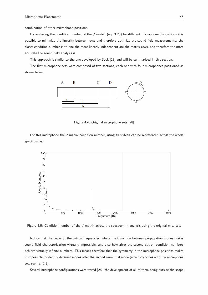
Microphone Placements 45
combination of other microphone positions.
By analyzing the condition number of the J matrix (eq. 3.23) for different microphone dispositions it ispossible to minimize the linearity between rows and therefore optimize the sound field measurements: thecloser condition number is to one the more linearly independent are the matrix rows, and therefore the moreaccurate the sound field analysis is
This approach is similar to the one developed by Sack [28] and will be summarized in this section:
The first microphone sets were composed of two sections, each one with four microphones positioned asshown below:
Figure 4.4: Original microphone sets [28]
For this microphone the J matrix condition number, using all sixteen can be represented across the wholespectrum as:
Figure 4.5: Condition number of the J matrix across the spectrum in analysis using the original mic. sets
Notice first the peaks at the cut-on frequencies, where the transition between propagation modes makessound field characterization virtually impossible, and also how after the second cut-on condition numbersachieve virtually infinite numbers. This means therefore that the symmetry in the microphone positions makesit impossible to identify different modes after the second azimuthal mode (which coincides with the microphoneset, see fig. 2.3).
Several microphone configurations were tested [28], the development of all of them being outside the scope

46 Facilities and Installation
of this thesis since its procedures were not taken at VKI or during my work in IDEALVENT. The chosenconfiguration was eventually the one presented in fig.
Figure 4.6: Final microphone positions, with α1 = α2 = 45° [28]
This microphone configuration, with 4 cm between each microphone section, provided the follwoing conditionnumbers acroos the spectrum in analysis:
Figure 4.7: Condition number of the J matrix across the spectrum in anaysis using the final microphone sets
As is the reader can see the condition numbers after the second cut-on now have acceptable values, meaningthe modal decomposition is possible and accurate. The continuous increase in the condition number across thespectrum is related to the fact that for higher order modes a higher number of microphones is needed. Thismeans that for lower order modes over-determination decreased drastically the matrix condition numbers butwhen higher order modes are included more microphones are required. Eventually, for the last range (plane waveplus first second and third azimuthal modes, plus the first radial mode) no over-determination is implementedsince those modes required all the microphones in presence.

Chapter 5
Reflection Matrices for Terminations:
Results
The calculation of the reflection matrix for both ends of the duct was carried out aiming to provide a simplifiedmethodology for the analysis of terminations without having to first study the two-port mid-duct problem. Forthis reason a rougher scale was used, with measurements being made every 100 Hz between 300 Hz and 3500Hz.
This methodology consisting of emitting different sinusoidal signals at different frequencies one at a time isusually referred as "step sine signal measurement", in opposition to the continuous "chirp signal" which evolvescontinuously from 0 Hz to a given frequency sweeping all the intermediate values [12].
Reflection matrices for the duct terminations were obtained by measuring the sound field at different pointsand then applying the methodologies presented in chapter 3. Since for different frequency ranges differentmodes are in presence the frequency spectrum in analysis was divided in five parts, each one delimited by itscut-on frequencies:
• Plane Wave Region:p′(x, r, θ) = (p+0,0e−ik
+
0,0x + p−0,0e+ik−
0,0x) f0,0(r)
• Plane Wave with First Azimuthal Mode:p′(x, r, θ) = ∑
+1m=−1 (p+m,0e−ik
+
m,0x + p−m,0e+ik−
m,0x) fm,0(r)eimθ
• Plane Wave with First and Second Azimuthal Modes:p′(x, r, θ) = ∑
+2m=−2 (p+m,0e−ik
+
m,0x + p−m,0e+ik−
m,0x) fm,0(r)eimθ
• Plane Wave with First and Second Azimuthal Modes and the First Radial Mode:p′(x, r, θ) = ∑
+2m=−2∑
1n=0 (p+m,ne−ik
+
m,nx + p−m,ne+ik−
m,nx) fm,n(r)eimθ
• Plane Wave with First Second and Third Azimuthal Modes and First Radial Mode:p′(x, r, θ) = ∑
+3m=−3∑
1n=0 (p+m,ne−ik
+
m,nx + p−m,ne+ik−
m,nx) fm,n(r)eimθ
The reflection process at the end of a duct includes not only the reflection of the emitted wave but alsoconversions in its modes. These reflective mechanisms very often give us information about how modes interact
47
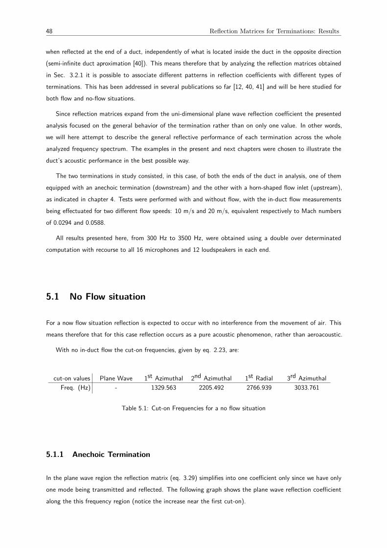
48 Reflection Matrices for Terminations: Results
when reflected at the end of a duct, independently of what is located inside the duct in the opposite direction(semi-infinite duct aproximation [40]). This means therefore that by analyzing the reflection matrices obtainedin Sec. 3.2.1 it is possible to associate different patterns in reflection coefficients with different types ofterminations. This has been addressed in several publications so far [12, 40, 41] and will be here studied forboth flow and no-flow situations.
Since reflection matrices expand from the uni-dimensional plane wave reflection coefficient the presentedanalysis focused on the general behavior of the termination rather than on only one value. In other words,we will here attempt to describe the general reflective performance of each termination across the wholeanalyzed frequency spectrum. The examples in the present and next chapters were chosen to illustrate theduct’s acoustic performance in the best possible way.
The two terminations in study consisted, in this case, of both the ends of the duct in analysis, one of themequipped with an anechoic termination (downstream) and the other with a horn-shaped flow inlet (upstream),as indicated in chapter 4. Tests were performed with and without flow, with the in-duct flow measurementsbeing effectuated for two different flow speeds: 10 m/s and 20 m/s, equivalent respectively to Mach numbersof 0.0294 and 0.0588.
All results presented here, from 300 Hz to 3500 Hz, were obtained using a double over determinatedcomputation with recourse to all 16 microphones and 12 loudspeakers in each end.
5.1 No Flow situation
For a now flow situation reflection is expected to occur with no interference from the movement of air. Thismeans therefore that for this case reflection occurs as a pure acoustic phenomenon, rather than aeroacoustic.
With no in-duct flow the cut-on frequencies, given by eq. 2.23, are:
cut-on values Plane Wave 1st Azimuthal 2nd Azimuthal 1st Radial 3rd AzimuthalFreq. (Hz) - 1329.563 2205.492 2766.939 3033.761
Table 5.1: Cut-on Frequencies for a no flow situation
5.1.1 Anechoic Termination
In the plane wave region the reflection matrix (eq. 3.29) simplifies into one coefficient only since we have onlyone mode being transmitted and reflected. The following graph shows the plane wave reflection coefficientalong the this frequency region (notice the increase near the first cut-on).

No Flow situation 49
Figure 5.1: Reflection coefficient of the Anechoic Termination in the plane wave region
After the cut-on at 1328.419 Hz we have in presence the first azimuthal modes. Thus we must now expandour representation to include the conversion coefficients
Figure 5.2: Reflection coefficients of the Anechoic Termination including plane wave and first azimuthal modes
One can observe the symmetry pattern between the first row coefficients, relative to the negative firstazimuthal mode and the third row coefficients, relative to the positive first azimuthal mode.
R11 and R33 are similar, meaning both first azimuthal modes are reflected as themselves in the same way.On the other hand R22, the reflection coefficient of the plane wave, displays a behavior independent of theother coefficients.

50 Reflection Matrices for Terminations: Results
For higher order modes it is no longer practical to represent reflection coefficients in plots as before givenits number, so it was decided to study reflection matrices by comparing their values directly. As an examplethe reflection matrix for 2500 Hz for the Anechoic Termination is shown below
R2500Hz =
⎡⎢⎢⎢⎢⎢⎢⎢⎢⎢⎢⎢⎢⎢⎢⎢⎣
0.3602 0.3196 0.1834 0.2109 0.1923
0.1874 0.3878 0.1701 0.3009 0.1116
0.0024 0.0674 0.1029 0.1246 0.0480
0.1027 0.1518 0.0837 0.3514 0.1579
0.3511 0.2559 0.1022 0.3733 0.3137
⎤⎥⎥⎥⎥⎥⎥⎥⎥⎥⎥⎥⎥⎥⎥⎥⎦
(5.1)
Once again it is possible to observe the similarity among the relative values within the diagonal, meaningmodes with different directions are reflected directly in the same way, with the independent value for the planewave direct reflection (underlined).
Between 2764.585 and 3031.168 Hz the computation must, as referred before, also include the propagationof the first radial mode. In this case, since this is not a spinning mode it will have assigned only one row andone column, with its direct reflection coefficient occupying the down right position.
The conversion coefficients related to radial-azimuthal interaction are denoted by the two rectangles in thematrix below,while the direct reflection coefficient for the first radial mode is also underlined:
R2900Hz =
0.2884 0.0394 0.1270 0.2171 0.0655 0.06850.0336 0.2690 0.0405 0.0402 0.1498 0.06120.0232 0.0927 0.2620 0.0363 0.1281 0.19750.0404 0.0752 0.0867 0.2678 0.0301 0.07220.0908 0.0672 0.0402 0.0402 0.3091 0.17230.3973 0.2213 0.2416 0.1516 0.1057 0.6175
⎡⎢⎢⎢⎢⎢⎢⎢⎢⎢⎢⎢⎢⎢⎢⎢⎣
⎤⎥⎥⎥⎥⎥⎥⎥⎥⎥⎥⎥⎥⎥⎥⎥⎦
(5.2)
Between 3031 and 3500 Hz, the last frequency range in study here, the third azimuthal mode must beincluded, this meaning that the matrix R will be 8 × 8 (2N + 1 +NR with N = 3 and NR = 1):
R3200Hz =
0.5832 0.1452 0.1418 0.3198 0.1968 0.0619 0.1369 0.26630.1433 0.2335 0.1313 0.0820 0.0703 0.2523 0.2049 0.09540.0349 0.0696 0.1873 0.1047 0.1634 0.0834 0.3115 0.13980.0809 0.1708 0.0244 0.2215 0.0700 0.0964 0.0175 0.08550.3234 0.0594 0.0634 0.0972 0.3153 0.0616 0.0217 0.09870.1059 0.0736 0.0736 0.1643 0.1371 0.2225 0.2697 0.09270.0827 0.1155 0.3016 0.2624 0.2203 0.3323 0.6099 0.12650.1539 0.1357 0.1915 0.4633 0.1323 0.1286 0.1653 0.5909
⎡⎢⎢⎢⎢⎢⎢⎢⎢⎢⎢⎢⎢⎢⎢⎢⎢⎢⎢⎢⎣
⎤⎥⎥⎥⎥⎥⎥⎥⎥⎥⎥⎥⎥⎥⎥⎥⎥⎥⎥⎥⎦
(5.3)
Where again the first radial mode related coefficients were highlighted.
5.1.2 Inlet
The same methodology adopted to represent results obtained for the anechoic termination can be used equallyto illustrate the results related to the flow inlet located on the upstream end of the duct.
The analysis will then start, as before, with the plane wave region, plotted in figure 5.3:

No Flow situation 51
Figure 5.3: Reflection coefficient of the inlet in the plane wave region
It is possible to notice the drop around 500 Hz as well as a rise as we draw closer to the first cut-on.
If we include the first azimuthal mode we will have the usual expansion presented in the following graph.Notice how convertive reflection coefficients are lower than their direct reflection counterparts:
Figure 5.4: Reflection coefficients for the inlet for plane wave and first azimuthal modes
For higher order modes the same matrix expansion can be performed:

52 Reflection Matrices for Terminations: Results
R2500Hz =
⎡⎢⎢⎢⎢⎢⎢⎢⎢⎢⎢⎢⎢⎢⎢⎢⎣
0.4314 0.2939 0.0189 0.1520 0.2621
0.0887 0.2825 0.0194 0.3015 0.0900
0.0038 0.1075 0.0951 0.0340 0.0116
0.1308 0.2501 0.1024 0.2956 0.1421
0.2642 0.2984 0.0122 0.1363 0.4919
⎤⎥⎥⎥⎥⎥⎥⎥⎥⎥⎥⎥⎥⎥⎥⎥⎦
(5.4)
Once again it is possible to observe the similarity among the values within the diagonal or at least intheir relative values, meaning modes with different directions are reflected directly in the same way, with theindependent value for the underline plane wave direct reflection.
Between 2764.585 and 3031.168 Hz the computation must, as referred before, also include the propagationof the first radial mode. As before it will have assigned only one row and one column, with its direct reflectioncoefficient occupying same the down right position.
The conversion coefficients related to radial-azimuthal interaction are again denoted by the two rectanglesin the matrix below:
R2900Hz =
0.1664 0.0492 0.0296 0.2227 0.1791 0.17220.0170 0.0139 0.0191 0.0218 0.1444 0.03990.0753 0.0536 0.0314 0.0807 0.0397 0.04080.0832 0.0109 0.0406 0.0347 0.0325 0.03910.0278 0.1423 0.0838 0.0513 0.1847 0.06590.0939 0.0480 0.3045 0.0831 0.3830 0.7123
⎡⎢⎢⎢⎢⎢⎢⎢⎢⎢⎢⎢⎢⎢⎢⎣
⎤⎥⎥⎥⎥⎥⎥⎥⎥⎥⎥⎥⎥⎥⎥⎦
(5.5)
Between 3031 and 3500 Hz, the last frequency interval in study here, the third azimuthal mode must beagain included,with the 8 × 8 matrix being given by:
R3300Hz =
0.5160 0.0876 0.0664 0.1466 0.1279 0.1336 0.1213 0.09390.0658 0.1500 0.1209 0.0345 0.0355 0.0850 0.0710 0.09260.0318 0.0706 0.0938 0.0313 0.0377 0.0785 0.1154 0.03050.0244 0.1047 0.0742 0.0898 0.0424 0.1898 0.0440 0.10490.1589 0.0563 0.0205 0.0083 0.0579 0.0171 0.0057 0.05380.0838 0.0646 0.0578 0.0287 0.0389 0.2372 0.1233 0.08520.0992 0.1493 0.1282 0.1644 0.0754 0.0210 0.4499 0.04830.0411 0.1498 0.0595 0.0874 0.1319 0.1725 0.1103 0.3792
⎡⎢⎢⎢⎢⎢⎢⎢⎢⎢⎢⎢⎢⎢⎢⎢⎢⎢⎢⎢⎣
⎤⎥⎥⎥⎥⎥⎥⎥⎥⎥⎥⎥⎥⎥⎥⎥⎥⎥⎥⎥⎦
(5.6)
Where again first radial mode related coefficients were highlighted.
5.1.3 Analysis
The analysis for each frequency range will follow the same approach as before:
For the plane wave region it can be observed from figures 5.3 and 5.6 that the reflection coefficient in thisrange is in fact lower for the inlet than for the anechoic terminaton. This can be justified if we observe theshape of both terminations:
The anechoic termination is composed of a set of resonators as referred in chapter 4 while the inlet is infact a horn-shaped termination. These two shapes are presented below:
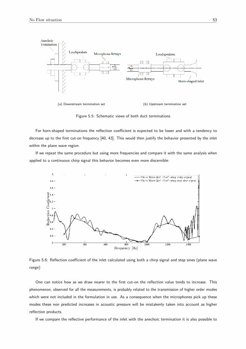
No Flow situation 53
(a) Downstream termination set (b) Upstream termination set
Figure 5.5: Schematic views of both duct terminations
For horn-shaped terminations the reflection coefficient is expected to be lower and with a tendency todecrease up to the first cut-on frequency [40, 43]. This would then justify the behavior presented by the inletwithin the plane wave region.
If we repeat the same procedure but using more frequencies and compare it with the same analysis whenapplied to a continuous chirp signal this behavior becomes even more discernible:
Figure 5.6: Reflection coefficient of the inlet calculated using both a chirp signal and step sines (plane waverange)
One can notice how as we draw nearer to the first cut-on the reflection value tends to increase. Thisphenomenon, observed for all the measurements, is probably related to the transmission of higher order modeswhich were not included in the formulation in use. As a consequence when the microphones pick up thesemodes these non predicted increases in acoustic pressure will be mistakenly taken into account as higherreflection products.
If we compare the reflective performance of the inlet with the anechoic termination it is also possible to

54 Reflection Matrices for Terminations: Results
observe how the resonator does not prevent reflection for lower frequencies in the same way they are reducedby the inlet horn-shaped geometry (compare, for example, the different reflection coefficients at 700 Hz).
If on the other hand we analyze the results obtained when we include the first azimuthal mode it becomesclear that not only the resonator minimizes reflections in a different way as also the terminations’ geometriesinduce different reflective patterns:
By comparing figs. 5.2 and 5.4 it is possible to note how R11 and R33 are similar not only in behavior butalso in value. This makes sense since the flow is considered to be at rest, therefore no spinning direction isfavored and both clockwise spinning and anti-clockwise spinning modes are reflected in the same way. This canbe observed at both terminations and would be expected to be related with the absence of non-axial flow.
It is also important to note how R13 and R31 follow in general similar patterns. This behavior of "crosssymmetry" means that opposite modes are converted in the same way between each other. Again it producesevidence of how no spinning direction is favored when reflection occurs at the upstream termination.
But perhaps the most important point to observe in these plots is the relation between the direct reflectioncoefficients and the so-called "convertive reflection coefficients": note how in fig. 5.4 the diagonal terms (R11,R22 and R33) are in general the higher values across the plane wave spectrum unlike the data in 5.6.
This effect is believed to be related with the fact that unlike the horn-shaped inlet the resonators in theanechoic termination do not constitute an axisymmetric geometry, and therefore modes are not conserved inthe their original forms since reflection is not homogeneous [41]. This can be understood by realizing how therectangular shape of the mufflers does not allow for modes to retain their original shapes since attenuationdoes not occur in an uniform way.
For higher order modes the composition of the reflection matrices provides us with the same type ofinformation and to some extent its analysis is carried out in the same way. For an easier analysis both matrices(anechoic termination (at) and inlet (i)) have here been replicated, this time only with the relevant valuesindicate, where the underlined value corresponds to the direct reflection coefficient for the plane wave mode:
R2500 Hzat=
⎡⎢⎢⎢⎢⎢⎢⎢⎢⎢⎢⎢⎢⎢⎢⎢⎣
0.3602 0.3196 0.1834 0.2109 0.1923
⋯ 0.3878 ⋯ 0.3009 ⋯
⋯ ⋯ 0.1029 0.1246 ⋯
⋯ ⋯ ⋯ 0.3514 ⋯
0.3511 0.2559 ⋯ 0.3733 0.3137
⎤⎥⎥⎥⎥⎥⎥⎥⎥⎥⎥⎥⎥⎥⎥⎥⎦
(5.7)
R2500 Hzi=
⎡⎢⎢⎢⎢⎢⎢⎢⎢⎢⎢⎢⎢⎢⎢⎢⎣
0.4314 0.2939 0.0189 0.1520 0.2621
⋯ 0.2825 ⋯ ⋯ ⋯
0.0038 0.1075 0.0951 0.0340 0.0116
⋯ ⋯ ⋯ 0.2956 ⋯
0.2642 0.2984 0.0122 0.1363 0.4919
⎤⎥⎥⎥⎥⎥⎥⎥⎥⎥⎥⎥⎥⎥⎥⎥⎦
(5.8)If we take the same approach as before but this time expanding our reasoning to the second azimuthal
modes we realize how the terms in the diagonal are similar and roughly symmetric around the center term(reflection coefficient of the planewave). Hence it should be noted how R11 is approximately equal to R55
for both matrices and once again for the inlet the terms within the diagonal are higher than any of theircounterparts in the same rows: notice how R11 and R55 are the higher values in the first and fifth rows.
Regarding symmetry it is possible to observe that the first and last rows in the reflection matrix of the inletare similar, indicating that reflection processes in similar ways for both directions as observed before.
Another effect in presence is how the non-diagonal terms in the reflection matrix of the anechoic terminationare higher than their inlet counterparts. For example, the R12 and R24 are higher in comparison to others
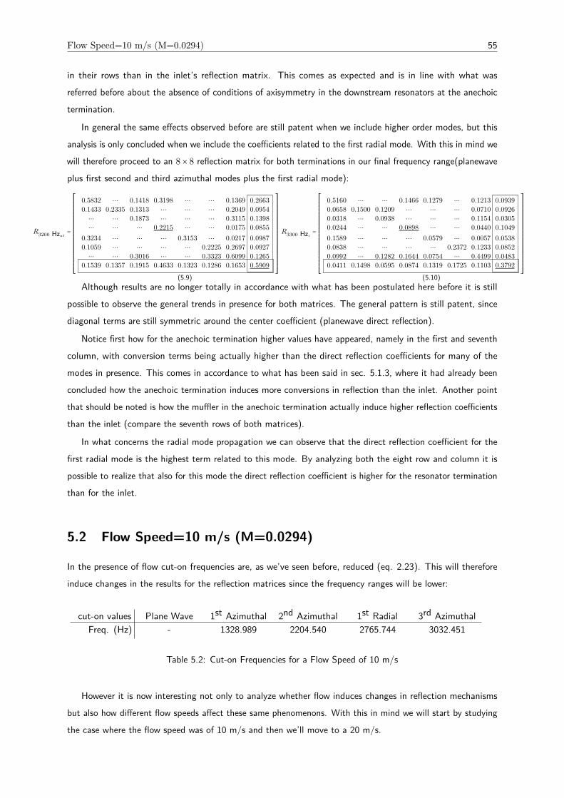
Flow Speed=10 m/s (M=0.0294) 55
in their rows than in the inlet’s reflection matrix. This comes as expected and is in line with what wasreferred before about the absence of conditions of axisymmetry in the downstream resonators at the anechoictermination.
In general the same effects observed before are still patent when we include higher order modes, but thisanalysis is only concluded when we include the coefficients related to the first radial mode. With this in mind wewill therefore proceed to an 8× 8 reflection matrix for both terminations in our final frequency range(planewaveplus first second and third azimuthal modes plus the first radial mode):
R3200 Hzat=
0.5832 ⋯ 0.1418 0.3198 ⋯ ⋯ 0.1369 0.26630.1433 0.2335 0.1313 ⋯ ⋯ ⋯ 0.2049 0.0954⋯ ⋯ 0.1873 ⋯ ⋯ ⋯ 0.3115 0.1398⋯ ⋯ ⋯ 0.2215 ⋯ ⋯ 0.0175 0.0855
0.3234 ⋯ ⋯ ⋯ 0.3153 ⋯ 0.0217 0.09870.1059 ⋯ ⋯ ⋯ ⋯ 0.2225 0.2697 0.0927⋯ ⋯ 0.3016 ⋯ ⋯ 0.3323 0.6099 0.1265
0.1539 0.1357 0.1915 0.4633 0.1323 0.1286 0.1653 0.5909
⎡⎢⎢⎢⎢⎢⎢⎢⎢⎢⎢⎢⎢⎢⎢⎢⎢⎢⎢⎢⎢⎣
⎤⎥⎥⎥⎥⎥⎥⎥⎥⎥⎥⎥⎥⎥⎥⎥⎥⎥⎥⎥⎥⎦
(5.9)
R3300 Hzi=
0.5160 ⋯ ⋯ 0.1466 0.1279 ⋯ 0.1213 0.09390.0658 0.1500 0.1209 ⋯ ⋯ ⋯ 0.0710 0.09260.0318 ⋯ 0.0938 ⋯ ⋯ ⋯ 0.1154 0.03050.0244 ⋯ ⋯ 0.0898 ⋯ ⋯ 0.0440 0.10490.1589 ⋯ ⋯ ⋯ 0.0579 ⋯ 0.0057 0.05380.0838 ⋯ ⋯ ⋯ ⋯ 0.2372 0.1233 0.08520.0992 ⋯ 0.1282 0.1644 0.0754 ⋯ 0.4499 0.04830.0411 0.1498 0.0595 0.0874 0.1319 0.1725 0.1103 0.3792
⎡⎢⎢⎢⎢⎢⎢⎢⎢⎢⎢⎢⎢⎢⎢⎢⎢⎢⎢⎢⎢⎣
⎤⎥⎥⎥⎥⎥⎥⎥⎥⎥⎥⎥⎥⎥⎥⎥⎥⎥⎥⎥⎥⎦
(5.10)Although results are no longer totally in accordance with what has been postulated here before it is still
possible to observe the general trends in presence for both matrices. The general pattern is still patent, sincediagonal terms are still symmetric around the center coefficient (planewave direct reflection).
Notice first how for the anechoic termination higher values have appeared, namely in the first and seventhcolumn, with conversion terms being actually higher than the direct reflection coefficients for many of themodes in presence. This comes in accordance to what has been said in sec. 5.1.3, where it had already beenconcluded how the anechoic termination induces more conversions in reflection than the inlet. Another pointthat should be noted is how the muffler in the anechoic termination actually induce higher reflection coefficientsthan the inlet (compare the seventh rows of both matrices).
In what concerns the radial mode propagation we can observe that the direct reflection coefficient for thefirst radial mode is the highest term related to this mode. By analyzing both the eight row and column it ispossible to realize that also for this mode the direct reflection coefficient is higher for the resonator terminationthan for the inlet.
5.2 Flow Speed=10 m/s (M=0.0294)
In the presence of flow cut-on frequencies are, as we’ve seen before, reduced (eq. 2.23). This will thereforeinduce changes in the results for the reflection matrices since the frequency ranges will be lower:
cut-on values Plane Wave 1st Azimuthal 2nd Azimuthal 1st Radial 3rd AzimuthalFreq. (Hz) - 1328.989 2204.540 2765.744 3032.451
Table 5.2: Cut-on Frequencies for a Flow Speed of 10 m/s
However it is now interesting not only to analyze whether flow induces changes in reflection mechanismsbut also how different flow speeds affect these same phenomenons. With this in mind we will start by studyingthe case where the flow speed was of 10 m/s and then we’ll move to a 20 m/s.

56 Reflection Matrices for Terminations: Results
One should notice that since the anechoic termination is located downstream the air flows inside the ductin the emitted wave’s direction while for the inlet located upstream the flow has the same direction as thereflected waves.
5.2.1 Anechoic Termination
A flow speed of 10 m/s is equivalent to a Mach number of 0.0294. This value, when included in computations,is not expected to induce significant changes. Indeed, by comparing fig. 5.6 with 5.7 it is possible to note thatthere has not major alterations in the reflection coefficient when flow was introduced in the duct.
Figure 5.7: Reflection coefficient of the Anechoic Termination in the plane wave region with M=0.0294
For the plane wave plus first azimuthal formulation results are once again similar to those obtained before,with the same patterns being displayed regardless of minor changes in values.

Flow Speed=10 m/s (M=0.0294) 57
Figure 5.8: Reflection coefficients of the Anechoic Termination for the plane wave and the first azimuthalmodes with M=0.0294
Moving on to the second azimuthal mode it is possible to observe that in the presence of flow directreflection coefficients for negative azimuthal modes have been reduced while their positive modes’ counterpartswere increased. The increase is also present in symmetrical reflections (coupling between opposite spinningmodes) since R15 is equal to R51 and R24 is equal to R42. The plane wave reflection coefficient has increased,but only slightly.
R2500Hz =
⎡⎢⎢⎢⎢⎢⎢⎢⎢⎢⎢⎢⎢⎢⎢⎢⎣
0.3447 0.3707 0.0763 0.2462 0.2834
0.2079 0.3786 0.1615 0.2875 0.1102
0.0159 0.0633 0.1047 0.1227 0.0451
0.1414 0.1412 0.0801 0.3701 0.1969
0.3926 0.2584 0.1088 0.3577 0.3480
⎤⎥⎥⎥⎥⎥⎥⎥⎥⎥⎥⎥⎥⎥⎥⎥⎦
(5.11)
If the first radial mode is included the increase in the diagonal values becomes more patent, while valuesfor the radial mode conversion coefficients appear to have been affected mildly. Overall the results appear toindicate the same patterns identified before.
R2900Hz =
0.3007 0.0490 0.1786 0.1611 0.0712 0.03760.0537 0.2796 0.0529 0.0458 0.1514 0.03390.0239 0.0943 0.2819 0.0579 0.1496 0.21780.0354 0.0986 0.0922 0.2697 0.0128 0.05870.1093 0.0548 0.0241 0.0621 0.3371 0.14030.4085 0.1629 0.2921 0.1361 0.1043 0.5812
⎡⎢⎢⎢⎢⎢⎢⎢⎢⎢⎢⎢⎢⎢⎢⎣
⎤⎥⎥⎥⎥⎥⎥⎥⎥⎥⎥⎥⎥⎥⎥⎦
(5.12)
Noticed how once again higher values for R38 R18 and R78 as well as R84 seem to indicate a couplingbetween the first radial mode and the third azimuthal mode as well as with the plane wave mode which can, in
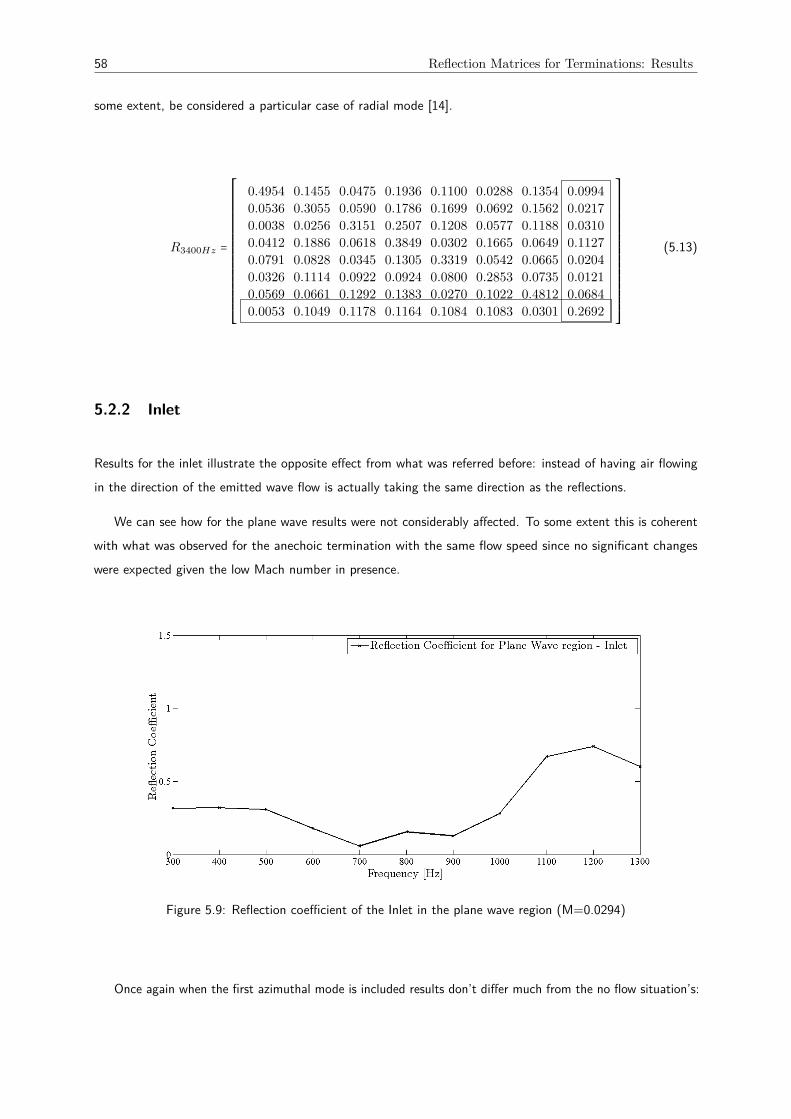
58 Reflection Matrices for Terminations: Results
some extent, be considered a particular case of radial mode [14].
R3400Hz =
0.4954 0.1455 0.0475 0.1936 0.1100 0.0288 0.1354 0.09940.0536 0.3055 0.0590 0.1786 0.1699 0.0692 0.1562 0.02170.0038 0.0256 0.3151 0.2507 0.1208 0.0577 0.1188 0.03100.0412 0.1886 0.0618 0.3849 0.0302 0.1665 0.0649 0.11270.0791 0.0828 0.0345 0.1305 0.3319 0.0542 0.0665 0.02040.0326 0.1114 0.0922 0.0924 0.0800 0.2853 0.0735 0.01210.0569 0.0661 0.1292 0.1383 0.0270 0.1022 0.4812 0.06840.0053 0.1049 0.1178 0.1164 0.1084 0.1083 0.0301 0.2692
⎡⎢⎢⎢⎢⎢⎢⎢⎢⎢⎢⎢⎢⎢⎢⎢⎢⎢⎢⎢⎣
⎤⎥⎥⎥⎥⎥⎥⎥⎥⎥⎥⎥⎥⎥⎥⎥⎥⎥⎥⎥⎦
(5.13)
5.2.2 Inlet
Results for the inlet illustrate the opposite effect from what was referred before: instead of having air flowingin the direction of the emitted wave flow is actually taking the same direction as the reflections.
We can see how for the plane wave results were not considerably affected. To some extent this is coherentwith what was observed for the anechoic termination with the same flow speed since no significant changeswere expected given the low Mach number in presence.
Figure 5.9: Reflection coefficient of the Inlet in the plane wave region (M=0.0294)
Once again when the first azimuthal mode is included results don’t differ much from the no flow situation’s:

Flow Speed=10 m/s (M=0.0294) 59
Figure 5.10: Reflection coefficients of the Inlet for plane and first azimuthal modes (M=0.0294)
For the inlet analysis with a flow speed of 10 m/s results remain similar to those obtained before, withvalues barely changing both within the diagonal and on the conversion terms except for those relative to theplane wave (third row and third column):
R2500Hz =
⎡⎢⎢⎢⎢⎢⎢⎢⎢⎢⎢⎢⎢⎢⎢⎢⎣
0.4210 0.2754 0.0429 0.2100 0.2710
0.0859 0.2758 0.0397 0.2836 0.1115
0.0115 0.1069 0.0877 0.0279 0.0064
0.1184 0.2495 0.1291 0.2684 0.1088
0.2591 0.2618 0.0053 0.1510 0.4963
⎤⎥⎥⎥⎥⎥⎥⎥⎥⎥⎥⎥⎥⎥⎥⎥⎦
(5.14)
By including the first radial (eq. 5.15) and the third azimuthal modes (eq. 5.16) we obtain the last twomatrices relative to this termination when in presence of a flow speed of 10 m/s.
It can be noted how the flow appears to have decreased significantly the radial mode’s coefficients whilemost of the direct reflection terms where in fact increased (with the exception of the their azimuthal mode).Some of the conversion values are now higher than their direct reflection counterparts, suggesting that thepresence of flow induces coupling between modes during reflection.
R3000Hz =
0.1505 0.0410 0.0233 0.0822 0.1822 0.07640.0258 0.1018 0.0317 0.0343 0.0535 0.02080.0317 0.0508 0.1133 0.0338 0.0287 0.09370.0937 0.0428 0.0437 0.0976 0.0497 0.01420.0506 0.1132 0.0393 0.0299 0.1731 0.01990.0647 0.0017 0.1193 0.0618 0.1869 0.4212
⎡⎢⎢⎢⎢⎢⎢⎢⎢⎢⎢⎢⎢⎢⎢⎣
⎤⎥⎥⎥⎥⎥⎥⎥⎥⎥⎥⎥⎥⎥⎥⎦
(5.15)

60 Reflection Matrices for Terminations: Results
R3400Hz =
0.5070 0.0851 0.0753 0.1142 0.0177 0.0560 0.0628 0.08080.0517 0.0672 0.0243 0.0859 0.0208 0.0369 0.1453 0.02740.0239 0.0433 0.0323 0.0857 0.0389 0.0380 0.1615 0.02660.0784 0.1312 0.0291 0.1589 0.0625 0.1164 0.0404 0.06030.0467 0.0724 0.0608 0.1284 0.0788 0.0937 0.0215 0.05830.0378 0.0591 0.0356 0.0801 0.0429 0.0671 0.1263 0.02060.0125 0.0726 0.0878 0.2060 0.0296 0.1084 0.5315 0.16150.1192 0.0687 0.0816 0.1770 0.0446 0.0822 0.0536 0.0933
⎡⎢⎢⎢⎢⎢⎢⎢⎢⎢⎢⎢⎢⎢⎢⎢⎢⎢⎢⎢⎣
⎤⎥⎥⎥⎥⎥⎥⎥⎥⎥⎥⎥⎥⎥⎥⎥⎥⎥⎥⎥⎦
(5.16)
5.2.3 Analysis
The results for the reflection matrices when flow is induced inside the duct provide a notion of how flow affectsthe acoustic phenomenons inside it. Unlike the previous case where all the studied events were only acousticallyrelated when flow is introduced inside the duct we have aeroacoustic mechanics in presence, which will allow usto understand how the speed of air affects reflection in this mean.
The main question is in fact how flow influences reflection when its direction is that of the emitted waveand when it is the same as that of the reflected signal.
With this in mind let us start by analyzing both figs 5.9 and 5.7 with 5.3 and 5.6. It is possible to noteflow has not changed the behavior of the planewave reflection coefficient and values are also similar.
This could however be justified by claiming that the Mach number was not high enough for its effects tomanifest explicitly. If we move on to including the first azimuthal mode it becomes clear once again that valueswere not significantly altered.
A more complete analysis is provided by including higher order modes. By analyzing both reflection matricesit is possible to realize how flow affects reflection:
R2500 Hzat=
⎡⎢⎢⎢⎢⎢⎢⎢⎢⎢⎢⎢⎢⎢⎢⎢⎣
0.3447 0.3707 0.0763 0.2462 0.2834
⋯ 0.3786 ⋯ 0.2875 ⋯
⋯ ⋯ 0.1047 0.1227 ⋯
⋯ 0.1412 ⋯ 0.3701 ⋯
0.3926 0.2584 ⋯ 0.3577 0.3480
⎤⎥⎥⎥⎥⎥⎥⎥⎥⎥⎥⎥⎥⎥⎥⎥⎦
(5.17)
R2500 Hzi=
⎡⎢⎢⎢⎢⎢⎢⎢⎢⎢⎢⎢⎢⎢⎢⎢⎣
0.4210 0.2754 0.0429 0.2100 0.2710
⋯ 0.2758 ⋯ ⋯ ⋯
0.0115 0.1069 0.0877 0.0279 0.0064
0.1184 ⋯ ⋯ 0.2684 ⋯
0.2591 0.2618 0.0053 0.1510 0.4963
⎤⎥⎥⎥⎥⎥⎥⎥⎥⎥⎥⎥⎥⎥⎥⎥⎦
(5.18)It can be noted that for the anechoic termination downstream the movement of air flowing in the direction
of the emitted waves appears to have decreased direct reflection coefficients for negative spinning modeswhile increasing their positive spinning counterparts (plane wave reflection coefficient remains similar). Thiswould mean that air flowing in the direction of the emitted waves reduces the reflection of negative modes asthemselves.
However it is possible to find convertive reflection coefficients which appear to have increased (R15 andRR51), this could mean therefore that flow decreases direct reflections and convertive reflections althoughit favors symmetrical reflections. Example of this is the fact that R15 and R24, as well as R24, increased.R42 decrease could be then considered a consequence of experimental methods and justified by stochasticunpredictable factors.
As for the inlet termination, where the flow follows the direction of reflected waves and reflection coefficients

Flowspeed=20 m/s (M=0.0588) 61
would be expected to increase it is interesting to observe that the values for direct reflection decreased whilethe convertive refection terms increased for the negative spinning modes some of them significantly (R13). Onthe other hand, for positive spinning modes convertive reflection coefficients dropped, such as R52 and R41.
This effect suggests that reflection does not process in the same way for all spinning modes. This makessense if we consider the possibility of vorticities in the flow that would favor the reflection of some modes (recallthat for the inlet the flow has the same directions as the reflected waves) and suppress the reflection of others.
Let us then evaluate this assumption when higher order modes are considered, now including both the thirdazimuthal modes and the first radial mode:
R3200 Hzat=
0.4954 ⋯ 0.0475 0.1936 ⋯ ⋯ 0.1354 0.09940.0536 0.3055 0.0590 ⋯ ⋯ ⋯ 0.1562 0.0217⋯ ⋯ 0.3151 ⋯ ⋯ ⋯ 0.1188 0.0310⋯ ⋯ ⋯ 0.3849 ⋯ ⋯ 0.0649 0.1127
0.0791 ⋯ ⋯ ⋯ 0.3319 ⋯ 0.0665 0.02040.0326 ⋯ ⋯ ⋯ ⋯ 0.2853 0.0735 0.0121⋯ ⋯ 0.1292 ⋯ ⋯ 0.1022 0.4812 0.0684
0.0053 0.1049 0.1178 0.1164 0.1084 0.1083 0.0301 0.2692
⎡⎢⎢⎢⎢⎢⎢⎢⎢⎢⎢⎢⎢⎢⎢⎢⎢⎢⎢⎢⎣
⎤⎥⎥⎥⎥⎥⎥⎥⎥⎥⎥⎥⎥⎥⎥⎥⎥⎥⎥⎥⎦
(5.19)
R3300 Hzi=
0.5070 ⋯ ⋯ 0.1142 0.0177 ⋯ 0.0628 0.08080.0517 0.0672 0.0243 ⋯ ⋯ ⋯ 0.1453 0.02740.0239 ⋯ 0.0323 ⋯ ⋯ ⋯ 0.1615 0.02660.0784 ⋯ ⋯ 0.1589 ⋯ ⋯ 0.0404 0.06030.0467 ⋯ ⋯ ⋯ 0.0788 ⋯ 0.0215 0.05830.0378 ⋯ ⋯ ⋯ ⋯ 0.0671 0.1263 0.02060.0125 ⋯ 0.0878 0.2060 0.0296 ⋯ 0.5315 0.16150.1192 0.0687 0.0816 0.1770 0.0446 0.0822 0.0536 0.0933
⎡⎢⎢⎢⎢⎢⎢⎢⎢⎢⎢⎢⎢⎢⎢⎢⎢⎢⎢⎢⎣
⎤⎥⎥⎥⎥⎥⎥⎥⎥⎥⎥⎥⎥⎥⎥⎥⎥⎥⎥⎥⎦
(5.20)
Starting our analysis by the anechoic termination we realize direct reflection coefficients are higher thanwhen no flow was present for the first and second azimuthal modes but lower for the third mode. On the otherhand the direct reflection coefficient for the first radial mode has decreased significantly from 0.5909 to 0.2692.Although this pattern seems to be difficult to understand it may once again indicate that the flow favors somemodes’ reflections and suppresses others’.
Convertive reflection coefficients decreased across the entire matrix, meaning that at higher frequenciesflow leaving the duct actually decreases convertive reflection at the escape termination.
The inlet’s performance at higher frequencies also seems to have been affected by the presence of flow,with a generalized drop in the values of direct reflection terms except for the plane wave, where a considerableincrease was registered. Although this would be potentially explained by the fact that air is flowing in thedirection of reflected waves it can’t be ignored that the direct reflection coefficient for the first radial mode issignificantly lower than that registered for the no flow case.
More important, this observation is not in line with what was postulated when the 5 × 5 matrices wereanalyzed, meaning that the reflection performance of terminations may vary with the frequencies considered.
Convertive reflection coefficients have also been generally reduced along the whole matrix, suggesting asbefore that for higher frequencies convertive reflections become weaker for lower order modes (notice that forthe third azimuthal mode the conversion terms are higher than for the lower order azimuthal modes).
5.3 Flowspeed=20 m/s (M=0.0588)
The final flow case in analysis was composed of the same 32 frequencies but this time with a flow speed of 20m/s, closer to the working condition of the ECS fan in study later on.
Since the results for flow measurements have already been analyzed and compared with those where noflow was induced inside the duct the present analysis aims to provide a notion of how an increase in flow speedaffects both terminations’ performances.

62 Reflection Matrices for Terminations: Results
The cut-on frequencies are once again here referred, this time for a flow speed of 20 m/s.
cut-on values Plane Wave 1st Azimuthal 2nd Azimuthal 1st Radial 3rd AzimuthalFreq. (Hz) - 1327.265 2201.680 2762.156 3028.517
Table 5.3: Cut-on Frequencies for a Flow Speed of 20 m/s
5.3.1 Anechoic Termination
The reflection coefficient in the plane wave range can still be represented using the same scale and limits sincethe change in cut-on frequencies is not significant. For the anechoic termination the results are still similar tothose without flow or with an in-duct flow of 10 m/s.
Figure 5.11: Reflection coefficient of the Anechoic Termination in the plane wave region (M=0.0588
If we now include the first azimuthal mode for the anechoic termination the results show that both termsR13 and R31 are now substantially increased. Note, however, that the general pattern remains the same:
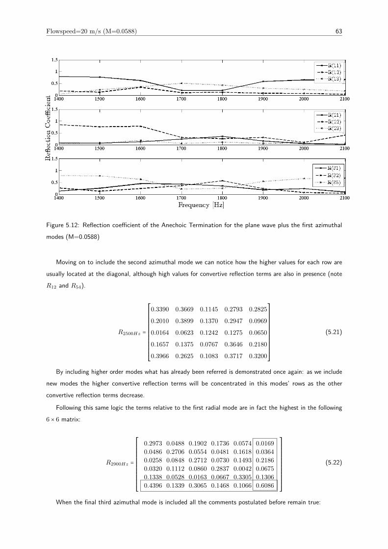
Flowspeed=20 m/s (M=0.0588) 63
Figure 5.12: Reflection coefficient of the Anechoic Termination for the plane wave plus the first azimuthalmodes (M=0.0588)
Moving on to include the second azimuthal mode we can notice how the higher values for each row areusually located at the diagonal, although high values for convertive reflection terms are also in presence (noteR12 and R54).
R2500Hz =
⎡⎢⎢⎢⎢⎢⎢⎢⎢⎢⎢⎢⎢⎢⎢⎢⎣
0.3390 0.3669 0.1145 0.2793 0.2825
0.2010 0.3899 0.1370 0.2947 0.0969
0.0164 0.0623 0.1242 0.1275 0.0650
0.1657 0.1375 0.0767 0.3646 0.2180
0.3966 0.2625 0.1083 0.3717 0.3200
⎤⎥⎥⎥⎥⎥⎥⎥⎥⎥⎥⎥⎥⎥⎥⎥⎦
(5.21)
By including higher order modes what has already been referred is demonstrated once again: as we includenew modes the higher convertive reflection terms will be concentrated in this modes’ rows as the otherconvertive reflection terms decrease.
Following this same logic the terms relative to the first radial mode are in fact the highest in the following6 × 6 matrix:
R2900Hz =
0.2973 0.0488 0.1902 0.1736 0.0574 0.01690.0486 0.2706 0.0554 0.0481 0.1618 0.03640.0258 0.0848 0.2712 0.0730 0.1493 0.21860.0320 0.1112 0.0860 0.2837 0.0042 0.06750.1338 0.0528 0.0163 0.0667 0.3305 0.13060.4396 0.1339 0.3065 0.1468 0.1066 0.6086
⎡⎢⎢⎢⎢⎢⎢⎢⎢⎢⎢⎢⎢⎢⎢⎣
⎤⎥⎥⎥⎥⎥⎥⎥⎥⎥⎥⎥⎥⎥⎥⎦
(5.22)
When the final third azimuthal mode is included all the comments postulated before remain true:

64 Reflection Matrices for Terminations: Results
R3400Hz =
0.4756 0.1091 0.0349 0.1238 0.0994 0.0270 0.1522 0.11050.0952 0.2761 0.0876 0.3734 0.2158 0.0293 0.2176 0.06850.0494 0.0136 0.3930 0.1214 0.1140 0.0423 0.1219 0.03510.0477 0.1420 0.0478 0.2331 0.0242 0.1278 0.0817 0.10520.1090 0.0604 0.0762 0.0735 0.3621 0.0300 0.0451 0.03830.0615 0.0712 0.0484 0.1187 0.1120 0.2271 0.1243 0.03530.0445 0.0343 0.0992 0.1702 0.0260 0.0694 0.4427 0.09850.0702 0.0634 0.0633 0.1362 0.1069 0.0846 0.0835 0.2492
⎡⎢⎢⎢⎢⎢⎢⎢⎢⎢⎢⎢⎢⎢⎢⎢⎢⎢⎢⎢⎣
⎤⎥⎥⎥⎥⎥⎥⎥⎥⎥⎥⎥⎥⎥⎥⎥⎥⎥⎥⎥⎦
(5.23)
5.3.2 Inlet
Results for the Inlet are next analyzed.
For the plane wave reflection coefficient once again results remain consistent, with no differences in thepattern and values similar to those of both no flow and flow speed of 10 m/s.
Figure 5.13: Reflection coefficient of the inlet in the plane wave region (M=0.0588)
If we include the first azimuthal mode the first difference between the anechoic termination and inlet with aflow speed of 20 m/s appears: notice how unlike in the case of the anechoic termination no reflection term hasincreased significantly, with the pattern remaining the same and the values close to those calculated before.
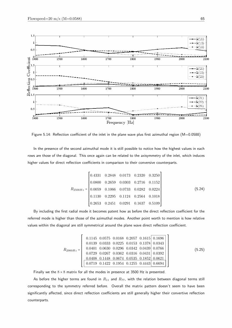
Flowspeed=20 m/s (M=0.0588) 65
Figure 5.14: Reflection coefficient of the inlet in the plane wave plus first azimuthal region (M=0.0588)
In the presence of the second azimuthal mode it is still possible to notice how the highest values in eachrows are those of the diagonal. This once again can be related to the axisymmetry of the inlet, which induceshigher values for direct reflection coefficients in comparison to their conversive counterparts.
R2500Hz =
⎡⎢⎢⎢⎢⎢⎢⎢⎢⎢⎢⎢⎢⎢⎢⎢⎣
0.4331 0.2848 0.0173 0.2320 0.3250
0.0800 0.2659 0.0303 0.2716 0.1152
0.0059 0.1066 0.0733 0.0282 0.0224
0.1130 0.2295 0.1124 0.2564 0.1018
0.2653 0.2451 0.0291 0.1637 0.5109
⎤⎥⎥⎥⎥⎥⎥⎥⎥⎥⎥⎥⎥⎥⎥⎥⎦
(5.24)
By including the first radial mode it becomes patent how as before the direct reflection coefficient for thereferred mode is higher than those of the azimuthal modes. Another point worth to mention is how relativevalues within the diagonal are still symmetrical around the plane wave direct reflection coefficient.
R2900Hz =
0.1145 0.0575 0.0168 0.2057 0.1615 0.16960.0139 0.0333 0.0225 0.0153 0.1378 0.03430.0401 0.0630 0.0296 0.0342 0.0439 0.07660.0729 0.0267 0.0362 0.0316 0.0431 0.03920.0408 0.1448 0.0674 0.0535 0.1852 0.06210.0719 0.1422 0.1954 0.1255 0.4443 0.6694
⎡⎢⎢⎢⎢⎢⎢⎢⎢⎢⎢⎢⎢⎢⎢⎣
⎤⎥⎥⎥⎥⎥⎥⎥⎥⎥⎥⎥⎥⎥⎥⎦
(5.25)
Finally we the 8 × 8 matrix for all the modes in presence at 3500 Hz is presented.
As before the higher terms are found in R11 and R77, with the relation between diagonal terms stillcorresponding to the symmetry referred before. Overall the matrix pattern doesn’t seem to have beensignificantly affected, since direct reflection coefficients are still generally higher their convertive reflectioncounterparts.
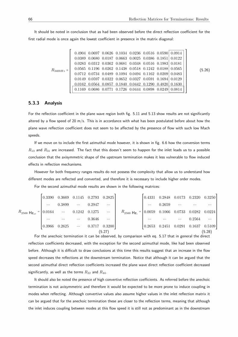
66 Reflection Matrices for Terminations: Results
It should be noted in conclusion that as had been observed before the direct reflection coefficient for thefirst radial mode is once again the lowest coefficient in presence in the matrix diagonal:
R3400Hz =
0.4904 0.0697 0.0626 0.1034 0.0236 0.0516 0.0590 0.09140.0389 0.0680 0.0187 0.0663 0.0025 0.0386 0.1851 0.01220.0283 0.0312 0.0362 0.0681 0.0348 0.0516 0.1983 0.01810.0565 0.1196 0.0262 0.1438 0.0518 0.1242 0.0188 0.05650.0712 0.0734 0.0489 0.1094 0.0494 0.1162 0.0209 0.04830.0149 0.0597 0.0322 0.0652 0.0327 0.0591 0.1694 0.01290.0162 0.0564 0.0857 0.1840 0.0442 0.1290 0.4820 0.16300.1169 0.0686 0.0771 0.1726 0.0444 0.0898 0.0249 0.0814
⎡⎢⎢⎢⎢⎢⎢⎢⎢⎢⎢⎢⎢⎢⎢⎢⎢⎢⎢⎢⎣
⎤⎥⎥⎥⎥⎥⎥⎥⎥⎥⎥⎥⎥⎥⎥⎥⎥⎥⎥⎥⎦
(5.26)
5.3.3 Analysis
For the reflection coefficient in the plane wave region both fig. 5.11 and 5.13 show results are not significantlyaltered by a flow speed of 20 m/s. This is in accordance with what has been postulated before about how theplane wave reflection coefficient does not seem to be affected by the presence of flow with such low Machspeeds.
If we move on to include the first azimuthal mode however, it is shown in fig. 6.6 how the conversion termsR13 and R31 are increased. The fact that this doesn’t seem to happen for the inlet leads us to a possibleconclusion that the axisymmetric shape of the upstream termination makes it less vulnerable to flow inducedeffects in reflection mechanisms.
However for both frequency ranges results do not possess the complexity that allow us to understand howdifferent modes are reflected and converted, and therefore it is necessary to include higher order modes.
For the second azimuthal mode results are shown in the following matrices:
R2500 Hzat=
⎡⎢⎢⎢⎢⎢⎢⎢⎢⎢⎢⎢⎢⎢⎢⎢⎣
0.3390 0.3669 0.1145 0.2793 0.2825
⋯ 0.3899 ⋯ 0.2947 ⋯
0.0164 ⋯ 0.1242 0.1275 ⋯
⋯ ⋯ ⋯ 0.3646 ⋯
0.3966 0.2625 ⋯ 0.3717 0.3200
⎤⎥⎥⎥⎥⎥⎥⎥⎥⎥⎥⎥⎥⎥⎥⎥⎦
(5.27)
R2500 Hzi=
⎡⎢⎢⎢⎢⎢⎢⎢⎢⎢⎢⎢⎢⎢⎢⎢⎣
0.4331 0.2848 0.0173 0.2320 0.3250
⋯ 0.2659 ⋯ ⋯ ⋯
0.0059 0.1066 0.0733 0.0282 0.0224
⋯ ⋯ ⋯ 0.2564 ⋯
0.2653 0.2451 0.0291 0.1637 0.5109
⎤⎥⎥⎥⎥⎥⎥⎥⎥⎥⎥⎥⎥⎥⎥⎥⎦
(5.28)For the anechoic termination it can be observed, by comparison with eq. 5.17 that in general the direct
reflection coefficients decreased, with the exception for the second azimuthal mode, like had been observedbefore. Although it is difficult to draw conclusions at this time this results suggest that an increase in the flowspeed decreases the reflections at the downstream termination. Notice that although it can be argued that thesecond azimuthal direct reflection coefficients increased the plane wave direct reflection coefficient decreasedsignificantly, as well as the terms R22 and R44.
It should also be noted the presence of high convertive reflection coefficients. As referred before the anechoictermination is not axisymmetric and therefore it would be expected to be more prone to induce coupling inmodes when reflecting. Although convertive values also assume higher values in the inlet reflection matrix itcan be argued that for the anechoic termination these are closer to the reflection terms, meaning that althoughthe inlet induces coupling between modes at this flow speed it is still not as predominant as in the downstream

Flowspeed=20 m/s (M=0.0588) 67
termination (compare for example the terms R31 or R13 in both matrices).Overall, the increase in the flow speed seems to have produced higher reflection coefficients, which was not
expected.The analysis is terminated when all three azimuthal modes are included, as well as the first radial mode:
R3200 Hzat=
0.4756 ⋯ 0.0349 0.1238 ⋯ ⋯ 0.1522 0.11050.0952 0.2761 0.0876 ⋯ ⋯ ⋯ 0.2176 0.0685⋯ ⋯ 0.3930 ⋯ ⋯ ⋯ 0.1219 0.0351⋯ ⋯ ⋯ 0.2331 ⋯ ⋯ 0.0817 0.1052
0.1090 ⋯ ⋯ ⋯ 0.3621 ⋯ 0.0451 0.03830.0615 ⋯ ⋯ ⋯ ⋯ 0.2271 0.1243 0.0353⋯ ⋯ 0.0992 ⋯ ⋯ 0.0694 0.4427 0.0985
0.0702 0.0634 0.0633 0.1362 0.1069 0.0846 0.0835 0.2492
⎡⎢⎢⎢⎢⎢⎢⎢⎢⎢⎢⎢⎢⎢⎢⎢⎢⎢⎢⎢⎣
⎤⎥⎥⎥⎥⎥⎥⎥⎥⎥⎥⎥⎥⎥⎥⎥⎥⎥⎥⎥⎦
(5.29)
R3300 Hzi=
0.4904 ⋯ ⋯ 0.1034 0.0236 ⋯ 0.0590 0.09140.0389 0.0680 0.0187 ⋯ ⋯ ⋯ 0.1851 0.01220.0283 ⋯ 0.0362 ⋯ ⋯ ⋯ 0.1983 0.01810.0565 ⋯ ⋯ 0.1438 ⋯ ⋯ 0.0188 0.05650.0712 ⋯ ⋯ ⋯ 0.0494 ⋯ 0.0209 0.04830.0149 ⋯ ⋯ ⋯ ⋯ 0.0591 0.1694 0.01290.0162 ⋯ 0.0857 0.1840 0.0442 ⋯ 0.4820 0.16300.1169 0.0686 0.0771 0.1726 0.0444 0.0898 0.0249 0.0814
⎡⎢⎢⎢⎢⎢⎢⎢⎢⎢⎢⎢⎢⎢⎢⎢⎢⎢⎢⎢⎣
⎤⎥⎥⎥⎥⎥⎥⎥⎥⎥⎥⎥⎥⎥⎥⎥⎥⎥⎥⎥⎦
(5.30)By analyzing the previous matrices it can be seen that the increase in flow speed lead to a decrease in
the direct reflection coefficients for the anechoic termination. This decrease was, however, accompanied byhigher values for the convertive reflection coefficients, namely in the seventh column (compare R67 with itscounterpart for flow speed equal to 10 m/s). This effect would therefore suggest that by increasing flow speedwe are in fact favoring convertive reflection over direct reflection, as terms outside the diagonal become higherand diagonal coefficients decrease.
On the other hand, values for the direct reflection coefficients in the reflection matrix of the inlet havedecreased too, with its convertive counterparts usually lower (effect of the axisymmetric [41]). It should be alsonoticed that convertive reflection coefficients have increased as had happened with the anechoic termination.
Finally, it is possible to observe that the terms relative to azimuthal modes display more complex behaviorsthan those of both the first radial mode and the plane wave. In fact only in the first radial mode terms wecould find consistence throughout the analysis: terms decreased as flow assumed higher velocities, retaininglower coefficients for the inlet than for the anechoic termination.

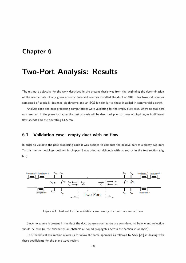
Chapter 6
Two-Port Analysis: Results
The ultimate objective for the work described in the present thesis was from the beginning the determinationof the source data of any given acoustic two-port sources installed the duct at VKI. This two-port sourcescomposed of specially designed diaphragms and an ECS fan similar to those installed in commercial aircraft.
Analysis code and post-processing computations were validating for the empty duct case, where no two-portwas inserted. In the present chapter this test analysis will be described prior to those of diaphragms in differentflow speeds and the operating ECS fan.
6.1 Validation case: empty duct with no flow
In order to validate the post-processing code it was decided to compute the passive part of a empty two-port.To this the methodology outlined in chapter 3 was adopted although with no source in the test section (fig.6.2)
Figure 6.1: Test set for the validation case: empty duct with no in-duct flow
Since no source is present in the duct the duct transmission factors are considered to be one and reflectionshould be zero (in the absence of an obstacle all sound propagates across the section in analysis).
This theoretical assumption allows us to follow the same approach as followed by Sack [28] in dealing withthese coefficients for the plane wave region:
69
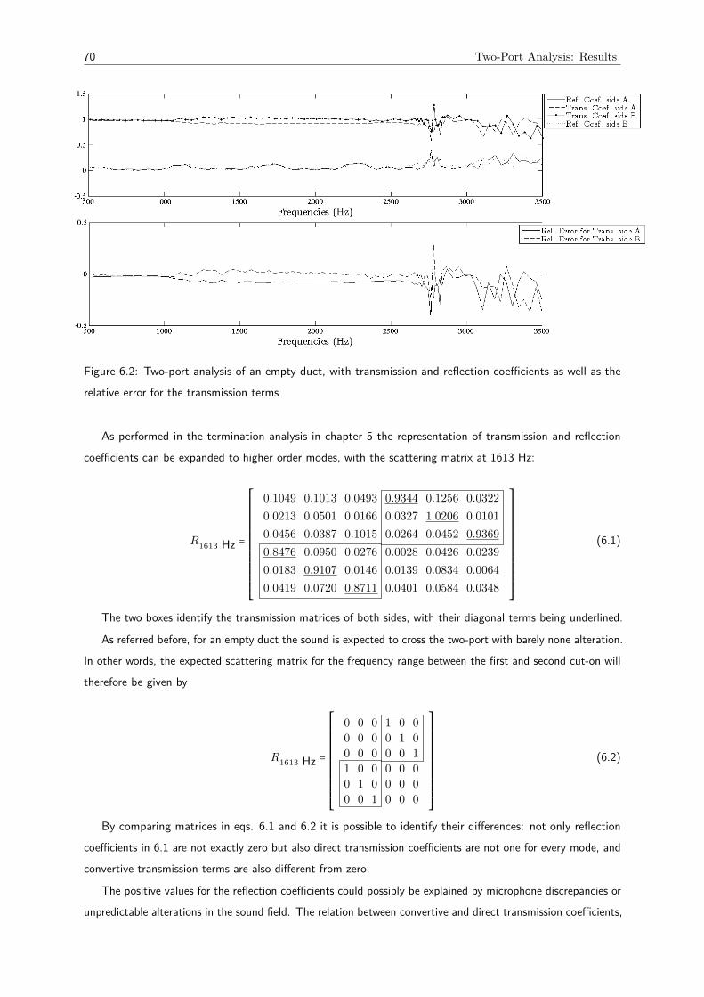
70 Two-Port Analysis: Results
Figure 6.2: Two-port analysis of an empty duct, with transmission and reflection coefficients as well as therelative error for the transmission terms
As performed in the termination analysis in chapter 5 the representation of transmission and reflectioncoefficients can be expanded to higher order modes, with the scattering matrix at 1613 Hz:
R1613 Hz =
0.1049 0.1013 0.0493 0.9344 0.1256 0.03220.0213 0.0501 0.0166 0.0327 1.0206 0.01010.0456 0.0387 0.1015 0.0264 0.0452 0.93690.8476 0.0950 0.0276 0.0028 0.0426 0.02390.0183 0.9107 0.0146 0.0139 0.0834 0.00640.0419 0.0720 0.8711 0.0401 0.0584 0.0348
⎡⎢⎢⎢⎢⎢⎢⎢⎢⎢⎢⎢⎢⎢⎢⎢⎢⎣
⎤⎥⎥⎥⎥⎥⎥⎥⎥⎥⎥⎥⎥⎥⎥⎥⎥⎦
(6.1)
The two boxes identify the transmission matrices of both sides, with their diagonal terms being underlined.
As referred before, for an empty duct the sound is expected to cross the two-port with barely none alteration.In other words, the expected scattering matrix for the frequency range between the first and second cut-on willtherefore be given by
R1613 Hz =
0 0 0 1 0 00 0 0 0 1 00 0 0 0 0 11 0 0 0 0 00 1 0 0 0 00 0 1 0 0 0
⎡⎢⎢⎢⎢⎢⎢⎢⎢⎢⎢⎢⎢⎢⎢⎣
⎤⎥⎥⎥⎥⎥⎥⎥⎥⎥⎥⎥⎥⎥⎥⎦
(6.2)
By comparing matrices in eqs. 6.1 and 6.2 it is possible to identify their differences: not only reflectioncoefficients in 6.1 are not exactly zero but also direct transmission coefficients are not one for every mode, andconvertive transmission terms are also different from zero.
The positive values for the reflection coefficients could possibly be explained by microphone discrepancies orunpredictable alterations in the sound field. The relation between convertive and direct transmission coefficients,

Diaphragm 71
however, can be explained by couplings between modes, which would therefore induce a decrease in directtransmission coefficients at the same time increasing the terms relative to mode conversion quantifying thecoupling between modes.
The same results were observed across the entire spectrum in study (500 to 3500 Hz), with reflectioncoefficients always lower then their transmission counterparts. More important, direct transmission termsalways close to one, thus validating the post-processing code in use for two-port analysis.
6.2 Diaphragm
Tests with a diaphragm in presence were performed with flow speeds of 10 and 20 m/s. The analysis includednot only the computation of the scattering matrix S of its passive part but also the active part, which quantifiedthe noise emitted by the diaphragm as an acoustic source.
The analysis of the passive part will be performed in a way similar to that in chapter 5, while the activepart will be addressed afterwards.
6.2.1 Without Flow
Analyzing the diaphragm’s acoustic performance when in the absence of flow makes it possible to betterunderstand how sound propagates across such a narrowing inside a duct.
On the other hand the passive part of a diaphragm in the absence of flow is somehow similar to the adoptedvalidation case of an empty duct equally without flow. On can think of a diaphragm as an obstacle included inthe validation case, and it is worth to take this into account along the analysis of the present case.
For the plane wane region transmission and reflection coefficients are shown in the following graph.
Figure 6.3: Passive part of the diaphragm in the absence of flow (plane wave region)
It can be observed that given its geometry the diaphragm presents transmission coefficients close to onethroughout most of the frequency range in study, with reflection coefficients being lower, in fact close tozero. Two other phenomenons can be observed: one regarding transmission terms, the other the reflection
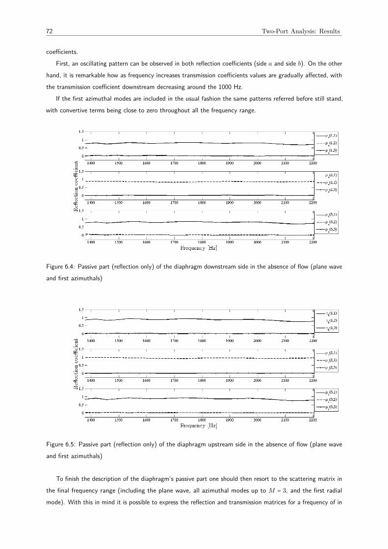
72 Two-Port Analysis: Results
coefficients.First, an oscillating pattern can be observed in both reflection coefficients (side a and side b). On the other
hand, it is remarkable how as frequency increases transmission coefficients values are gradually affected, withthe transmission coefficient downstream decreasing around the 1000 Hz.
If the first azimuthal modes are included in the usual fashion the same patterns referred before still stand,with convertive terms being close to zero throughout all the frequency range.
Figure 6.4: Passive part (reflection only) of the diaphragm downstream side in the absence of flow (plane waveand first azimuthals)
Figure 6.5: Passive part (reflection only) of the diaphragm upstream side in the absence of flow (plane waveand first azimuthals)
To finish the description of the diaphragm’s passive part one should then resort to the scattering matrix inthe final frequency range (including the plane wave, all azimuthal modes up to M = 3, and the first radialmode). With this in mind it is possible to express the reflection and transmission matrices for a frequency of in

Diaphragm 73
the following way:
ρa3501 Hz =
0.7113 0.0550 0.0165 0.1605 0.0211 0.0236 0.0492 0.04050.1356 0.7408 0.1318 0.0890 0.1117 0.0528 0.0384 0.04520.0527 0.1136 0.6776 0.3084 0.0634 0.0784 0.1250 0.06460.0535 0.0335 0.0079 0.4758 0.0647 0.0119 0.0143 0.35490.1232 0.0536 0.0686 0.5186 0.5657 0.0177 0.1127 0.02350.1428 0.0430 0.1392 0.1165 0.0803 0.7371 0.0288 0.03140.0633 0.0521 0.0283 0.2289 0.0459 0.0361 0.6456 0.01650.0206 0.1451 0.0683 0.6597 0.0197 0.1630 0.0571 0.3019
⎡⎢⎢⎢⎢⎢⎢⎢⎢⎢⎢⎢⎢⎢⎢⎢⎢⎢⎢⎢⎣
⎤⎥⎥⎥⎥⎥⎥⎥⎥⎥⎥⎥⎥⎥⎥⎥⎥⎥⎥⎥⎦
(6.3)
ρb3501 Hz =
0.6949 0.0668 0.0270 0.0494 0.0382 0.0370 0.0300 0.02530.0775 0.8168 0.1724 0.1245 0.1400 0.0553 0.0701 0.04140.0465 0.0508 0.6974 0.2079 0.0973 0.0356 0.1080 0.06280.0401 0.1576 0.0319 0.2975 0.0979 0.1469 0.0063 0.48250.0832 0.1158 0.0574 0.0294 0.5814 0.1030 0.0019 0.00840.0771 0.1098 0.1575 0.1196 0.1215 0.6936 0.0842 0.04100.0133 0.0168 0.0523 0.0544 0.0318 0.0077 0.6983 0.01580.0283 0.1156 0.0506 0.6996 0.0662 0.1275 0.0149 0.3051
⎡⎢⎢⎢⎢⎢⎢⎢⎢⎢⎢⎢⎢⎢⎢⎢⎢⎢⎢⎢⎣
⎤⎥⎥⎥⎥⎥⎥⎥⎥⎥⎥⎥⎥⎥⎥⎥⎥⎥⎥⎥⎦
(6.4)
It can concluded from eqs. 6.3 and 6.4 that direct reflections are favored in detriment of their convertivecounterparts. This is in agreement with what hed been referred in chapter 5 about how axisimmetry inducesthis pattern of direct terms being higher than convertive terms [40].
On the other hand, the fact that reflection coefficients are the same for both sides (discount a slightincrease in upstream values in comparison with the downstream terms) suggests yet another between a two-portsymmetry and its acoustic performance. The fact that this symmetry holds for the first radial mode for bothconvertive and direct terms confirms this same assumption.
Of course this description is not complete without performing the same analysis for transmission terms:
τa3501 Hz =
0.3920 0.0029 0.0420 0.1751 0.0119 0.0176 0.0437 0.00930.0236 0.5123 0.0900 0.2149 0.0829 0.0537 0.0271 0.01300.0156 0.0496 0.6241 0.0413 0.0580 0.0477 0.0973 0.03840.0263 0.0753 0.0368 0.4886 0.0328 0.0606 0.0155 0.19640.0528 0.0205 0.1088 0.2833 0.5746 0.0328 0.0391 0.04000.0675 0.0095 0.0806 0.2275 0.0466 0.5206 0.0197 0.05190.0125 0.0052 0.0118 0.0483 0.0521 0.0328 0.4020 0.01590.0237 0.0313 0.0681 0.2974 0.0079 0.0145 0.0230 0.7256
⎡⎢⎢⎢⎢⎢⎢⎢⎢⎢⎢⎢⎢⎢⎢⎢⎢⎢⎢⎢⎣
⎤⎥⎥⎥⎥⎥⎥⎥⎥⎥⎥⎥⎥⎥⎥⎥⎥⎥⎥⎥⎦
(6.5)
τb3501 Hz =
0.3537 0.0669 0.0051 0.0923 0.0162 0.0235 0.0447 0.01260.0761 0.5809 0.0807 0.0783 0.0419 0.0404 0.0205 0.01650.0596 0.1006 0.6115 0.5153 0.0938 0.0589 0.1536 0.04040.0247 0.0780 0.0171 0.6250 0.0121 0.0393 0.0184 0.10690.0846 0.0431 0.0275 0.0754 0.6286 0.0348 0.0219 0.06970.0557 0.0818 0.0918 0.0643 0.0305 0.4999 0.0326 0.03000.0210 0.0278 0.0323 0.1406 0.0293 0.0190 0.3826 0.02390.0470 0.1013 0.0438 0.5373 0.0345 0.0852 0.0892 0.6724
⎡⎢⎢⎢⎢⎢⎢⎢⎢⎢⎢⎢⎢⎢⎢⎢⎢⎢⎢⎢⎣
⎤⎥⎥⎥⎥⎥⎥⎥⎥⎥⎥⎥⎥⎥⎥⎥⎥⎥⎥⎥⎦
(6.6)
The results are in some way an extension of what had already been observed for reflection terms in eqs. 6.3and 6.4: once again the patterns show higher direct coefficients and lower convertive terms, at the same timematrices are similar in values, thus corroborating what had been suggested before about symmetry effects.
To conclude this description it should be noted the slight increase in values in the τb matrix in comparisonwith its τa counterparts.
Analysis
The analysis of the diaphragm with no flow case is simplified by the results’ concordance with what was alreadyexpected: coefficients are higher for direct terms than convertive terms, assuming values similar in both sides,confirming the symmetry character of the two-port.
More important, for lower frequencies the diaphragm is "virtually" transparent to acoustic waves (ρ = 0,τ = 1). This is in agreement with what has been suggested by Sack [28], and illustrates how lower order modsare not as sensitive to axissimetrical obstacles as their higher order counterparts.
Higher values for upstream transition terms may be relative with possible parasitic flow disturbances reportedduring experiences related to occasional pressure differences between both sides of the anechoic chamber.
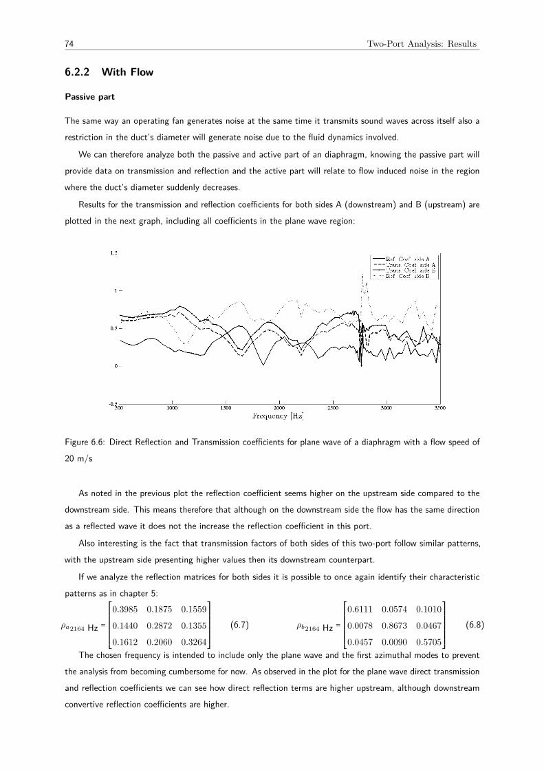
74 Two-Port Analysis: Results
6.2.2 With Flow
Passive part
The same way an operating fan generates noise at the same time it transmits sound waves across itself also arestriction in the duct’s diameter will generate noise due to the fluid dynamics involved.
We can therefore analyze both the passive and active part of an diaphragm, knowing the passive part willprovide data on transmission and reflection and the active part will relate to flow induced noise in the regionwhere the duct’s diameter suddenly decreases.
Results for the transmission and reflection coefficients for both sides A (downstream) and B (upstream) areplotted in the next graph, including all coefficients in the plane wave region:
Figure 6.6: Direct Reflection and Transmission coefficients for plane wave of a diaphragm with a flow speed of20 m/s
As noted in the previous plot the reflection coefficient seems higher on the upstream side compared to thedownstream side. This means therefore that although on the downstream side the flow has the same directionas a reflected wave it does not the increase the reflection coefficient in this port.
Also interesting is the fact that transmission factors of both sides of this two-port follow similar patterns,with the upstream side presenting higher values then its downstream counterpart.
If we analyze the reflection matrices for both sides it is possible to once again identify their characteristicpatterns as in chapter 5:
ρa2164 Hz =
⎡⎢⎢⎢⎢⎢⎢⎢⎢⎣
0.3985 0.1875 0.1559
0.1440 0.2872 0.1355
0.1612 0.2060 0.3264
⎤⎥⎥⎥⎥⎥⎥⎥⎥⎦
(6.7) ρb2164 Hz =
⎡⎢⎢⎢⎢⎢⎢⎢⎢⎣
0.6111 0.0574 0.1010
0.0078 0.8673 0.0467
0.0457 0.0090 0.5705
⎤⎥⎥⎥⎥⎥⎥⎥⎥⎦
(6.8)
The chosen frequency is intended to include only the plane wave and the first azimuthal modes to preventthe analysis from becoming cumbersome for now. As observed in the plot for the plane wave direct transmissionand reflection coefficients we can see how direct reflection terms are higher upstream, although downstreamconvertive reflection coefficients are higher.

Diaphragm 75
If on the other hand we analyze transmission values we’ll have, for the same frequency:
τa3541 Hz =
⎡⎢⎢⎢⎢⎢⎢⎢⎢⎣
0.5307 0.1299 0.1269
0.0487 0.2498 0.0221
0.1009 0.1381 0.4883
⎤⎥⎥⎥⎥⎥⎥⎥⎥⎦
(6.9) τb3541 Hz =
⎡⎢⎢⎢⎢⎢⎢⎢⎢⎣
0.5327 0.0478 0.1141
0.0954 0.3406 0.1030
0.1016 0.0591 0.6485
⎤⎥⎥⎥⎥⎥⎥⎥⎥⎦
(6.10)
Where it is possible to notice how values are now considerably more similar in comparison to the matricesin eqs. 6.7 and 6.8. Notice also the higher values in both being observed for direct coefficients.
For the sake of completion this section will be concluded with the total expansions, including the planewave, azimuthal modes, and also the first radial mode:
ρa3541 Hz =
0.2110 0.1239 0.0928 0.1838 0.3877 0.0865 0.0786 0.04230.2394 0.2089 0.1982 0.3100 0.1504 0.0805 0.1324 0.11080.0542 0.0322 0.4780 0.2674 0.1612 0.1430 0.0660 0.01640.0547 0.0976 0.1131 0.2605 0.2513 0.1016 0.0207 0.35010.1661 0.0908 0.2928 0.3497 0.4550 0.1458 0.0388 0.00950.1528 0.0596 0.1175 0.2132 0.1478 0.3126 0.0780 0.02700.0346 0.0058 0.0515 0.1137 0.0263 0.0946 0.1228 0.02060.0430 0.1086 0.0191 0.6553 0.0207 0.0884 0.0537 0.6155
⎡⎢⎢⎢⎢⎢⎢⎢⎢⎢⎢⎢⎢⎢⎢⎢⎢⎢⎢⎢⎢⎢⎢⎣
⎤⎥⎥⎥⎥⎥⎥⎥⎥⎥⎥⎥⎥⎥⎥⎥⎥⎥⎥⎥⎥⎥⎥⎦
(6.11)
ρb3541 Hz =
0.2630 0.1477 0.1857 0.4289 0.2750 0.1980 0.1533 0.09200.1806 0.4146 0.1232 0.2509 0.4298 0.1240 0.0987 0.02520.0887 0.1590 0.5196 0.3513 0.2437 0.2691 0.1649 0.05780.0715 0.0618 0.1208 0.8720 0.0367 0.1092 0.2011 0.37570.0938 0.1815 0.0448 0.2573 0.3910 0.1943 0.0601 0.05030.0748 0.1446 0.1061 0.1090 0.1508 0.2875 0.2414 0.08220.0828 0.0429 0.1400 0.3122 0.2286 0.0951 0.2861 0.10640.0867 0.2964 0.1220 0.6099 0.2837 0.4502 0.1016 0.6122
⎡⎢⎢⎢⎢⎢⎢⎢⎢⎢⎢⎢⎢⎢⎢⎢⎢⎢⎢⎢⎢⎢⎢⎣
⎤⎥⎥⎥⎥⎥⎥⎥⎥⎥⎥⎥⎥⎥⎥⎥⎥⎥⎥⎥⎥⎥⎥⎦
(6.12)
It is here worth to notice how although the direct reflection coefficient for the first radial mode is in factsimilar for both sides its convertive coefficient are actually very different. Another point worth to mention ishow the tendency of direct reflection coefficients (underlined) for being higher upstream than downstream stillholds for higher frequencies and higher order modes.
The same results, except this time for transmission terms, are shown next, where the similarities among thematrices’ values can again be noted.
τa3541 Hz =
0.5620 0.0522 0.1733 0.3322 0.2265 0.1375 0.0718 0.04950.1796 0.5734 0.2160 0.2806 0.3229 0.0899 0.0924 0.08180.0784 0.0748 0.5277 0.1783 0.3368 0.0377 0.0793 0.02820.0622 0.0708 0.1350 0.3379 0.0759 0.0697 0.0527 0.13030.1510 0.1308 0.2191 0.2825 0.6491 0.1595 0.0815 0.08170.1002 0.0273 0.0534 0.3096 0.1033 0.5732 0.0275 0.05700.2513 0.1241 0.4958 0.4906 0.4109 0.1621 0.4277 0.05360.0690 0.1009 0.1533 0.2883 0.1248 0.1108 0.1091 0.1931
⎡⎢⎢⎢⎢⎢⎢⎢⎢⎢⎢⎢⎢⎢⎢⎢⎢⎢⎢⎢⎢⎢⎢⎣
⎤⎥⎥⎥⎥⎥⎥⎥⎥⎥⎥⎥⎥⎥⎥⎥⎥⎥⎥⎥⎥⎥⎥⎦
(6.13)
τb3541 Hz =
0.5539 0.2679 0.3757 0.8315 0.3548 0.3132 0.2181 0.10320.1347 0.5999 0.1187 0.4237 0.2146 0.0383 0.1171 0.10180.0657 0.1062 0.5701 0.3477 0.1660 0.1556 0.1122 0.04010.1281 0.0359 0.1071 0.5234 0.1780 0.1265 0.0981 0.41070.1421 0.2675 0.1368 0.3893 0.8077 0.3088 0.0211 0.07850.0434 0.1962 0.0796 0.2096 0.0477 0.7730 0.1784 0.03080.0155 0.0402 0.0509 0.1981 0.1045 0.1871 0.7386 0.05450.0606 0.0306 0.1103 0.3440 0.1041 0.0636 0.0195 0.2776
⎡⎢⎢⎢⎢⎢⎢⎢⎢⎢⎢⎢⎢⎢⎢⎢⎢⎢⎢⎢⎢⎢⎢⎣
⎤⎥⎥⎥⎥⎥⎥⎥⎥⎥⎥⎥⎥⎥⎥⎥⎥⎥⎥⎥⎥⎥⎥⎦
(6.14)
Active part
As referred before, in the presence of flow the diaphragm generates noise, mostly due to the generation ofvorticities in its boundaries. Having calculated the passive part of this two-port source, it is now time tocompute its active part.
In fig. 6.8 the computed active part was superimposed on the sound field measurements by microphone16 on the upstream side of the diaphragm, in order to allow a comparison between both values for differentfrequencies.

76 Two-Port Analysis: Results
Figure 6.7: Diaphragm’s active part with total measured pressure on both sides a and b
It is worth mentioning the discrepancy between the plane wave amplitude (broken line) over the continuousline relative to the recorded sound pressure level. It is therefore expected for the plane wave amplitude to behigher than the overall sound pressure level for most of the frequencies, since the SPL includes the phase atthe microphone positions, regarding axial azimuthal and radial coordinates (recall eq. 2.14). It is also worthnoticing how the discrepancy decreases as the frequency increases, given the appearance of other modes.
6.2.3 Analysis
The analysis of the two-port results for a diaphragm in presence of flow must start with its passive part.
In what concerns reflection terms it must be noted how for the downstream side direct reflection coefficientsare lower than on the upstream side. However, we cannot ignore that convertive reflection appears to bemore preponderant downstream than upstream for lower frequencies (recall eqs. 6.7 and 6.8) while for higherfrequencies this conclusion does not seem to be that straightforward.
Notice however how in eqs. 6.7 and 6.8 convertive values are this time higher upstream than downstream,thus meaning that the relation between values on both sides of the two-port varies with frequency.
Perhaps the most interesting data resides in the first radial mode, where although the direct reflectioncoefficient does not differ by more than 0.033 the convertive reflection coefficients significantly higher upstream,suggesting that on the upstream side of the diaphragm reflection is definitely stronger than downstream.
Regarding transmission terms results are in fact more consistent with what was observed at lower frequencies.It is possible to notice how direct transmission coefficients are higher for the upstream side rather than for itsdownstream counterpart. In a way, this comes related to what has been referred before about flow having thesame direction as original emitted waves inducing higher transmission coefficients.
The calculated plane wave acoustic pressure generated by the source proved to follow the same tendency asthe recorded SPL, which seems plausible and follows the initial expectations.
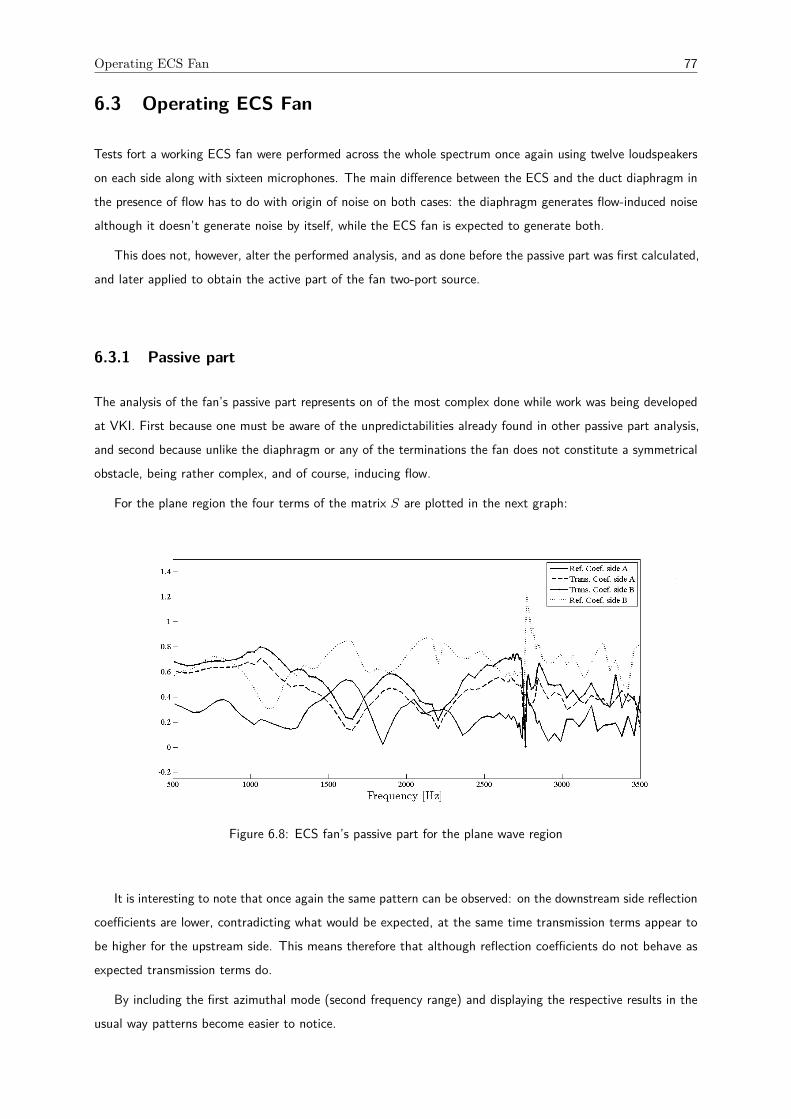
Operating ECS Fan 77
6.3 Operating ECS Fan
Tests fort a working ECS fan were performed across the whole spectrum once again using twelve loudspeakerson each side along with sixteen microphones. The main difference between the ECS and the duct diaphragm inthe presence of flow has to do with origin of noise on both cases: the diaphragm generates flow-induced noisealthough it doesn’t generate noise by itself, while the ECS fan is expected to generate both.
This does not, however, alter the performed analysis, and as done before the passive part was first calculated,and later applied to obtain the active part of the fan two-port source.
6.3.1 Passive part
The analysis of the fan’s passive part represents on of the most complex done while work was being developedat VKI. First because one must be aware of the unpredictabilities already found in other passive part analysis,and second because unlike the diaphragm or any of the terminations the fan does not constitute a symmetricalobstacle, being rather complex, and of course, inducing flow.
For the plane region the four terms of the matrix S are plotted in the next graph:
Figure 6.8: ECS fan’s passive part for the plane wave region
It is interesting to note that once again the same pattern can be observed: on the downstream side reflectioncoefficients are lower, contradicting what would be expected, at the same time transmission terms appear tobe higher for the upstream side. This means therefore that although reflection coefficients do not behave asexpected transmission terms do.
By including the first azimuthal mode (second frequency range) and displaying the respective results in theusual way patterns become easier to notice.
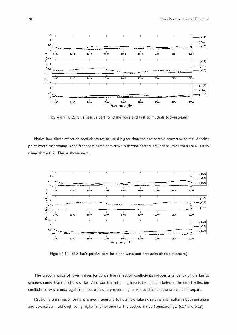
78 Two-Port Analysis: Results
Figure 6.9: ECS fan’s passive part for plane wave and first azimuthals (downstream)
Notice how direct reflection coefficients are as usual higher than their respective convertive terms. Anotherpoint worth mentioning is the fact these same convertive reflection factors are indeed lower than usual, rarelyrising above 0.2. This is shown next:
Figure 6.10: ECS fan’s passive part for plane wave and first azimuthals (upstream)
The predominance of lower values for convertive reflection coefficients induces a tendency of the fan tosuppress convertive reflections so far. Also worth mentioning here is the relation between the direct reflectioncoefficients, where once again the upstream side presents higher values that its downstream counterpart.
Regarding transmission terms it is now interesting to note how values display similar patterns both upstreamand downstream, although being higher in amplitude for the upstream side (compare figs. 6.17 and 6.18).
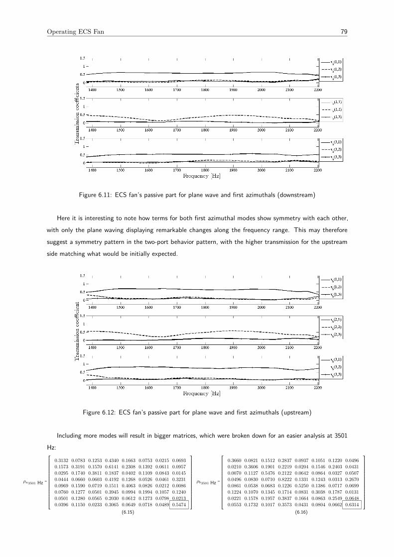
Operating ECS Fan 79
Figure 6.11: ECS fan’s passive part for plane wave and first azimuthals (downstream)
Here it is interesting to note how terms for both first azimuthal modes show symmetry with each other,with only the plane waving displaying remarkable changes along the frequency range. This may thereforesuggest a symmetry pattern in the two-port behavior pattern, with the higher transmission for the upstreamside matching what would be initially expected.
Figure 6.12: ECS fan’s passive part for plane wave and first azimuthals (upstream)
Including more modes will result in bigger matrices, which were broken down for an easier analysis at 3501Hz:
ρa3501 Hz =
0.3132 0.0783 0.1253 0.4340 0.1663 0.0753 0.0215 0.06930.1573 0.3191 0.1570 0.6141 0.2308 0.1392 0.0611 0.09570.0295 0.1740 0.3811 0.1837 0.0402 0.1109 0.0843 0.01450.0444 0.0660 0.0603 0.4192 0.1268 0.0526 0.0461 0.32310.0969 0.1590 0.0719 0.1511 0.4063 0.0826 0.0212 0.00860.0760 0.1277 0.0501 0.3945 0.0994 0.1994 0.1057 0.12400.0501 0.1280 0.0565 0.2030 0.0612 0.1273 0.0798 0.02130.0396 0.1150 0.0233 0.3065 0.0649 0.0718 0.0489 0.5474
⎡⎢⎢⎢⎢⎢⎢⎢⎢⎢⎢⎢⎢⎢⎢⎢⎢⎢⎢⎢⎣
⎤⎥⎥⎥⎥⎥⎥⎥⎥⎥⎥⎥⎥⎥⎥⎥⎥⎥⎥⎥⎦
(6.15)
ρb3501 Hz =
0.3660 0.0821 0.1512 0.2837 0.0937 0.1051 0.1220 0.04960.0210 0.3606 0.1901 0.2219 0.0204 0.1546 0.2403 0.04310.0070 0.1127 0.5476 0.2122 0.0642 0.0864 0.0327 0.05070.0496 0.0830 0.0710 0.8222 0.1331 0.1243 0.0313 0.26700.0861 0.0538 0.0683 0.1226 0.5250 0.1386 0.0717 0.06990.1224 0.1070 0.1345 0.1714 0.0831 0.3038 0.1787 0.01310.0221 0.1578 0.1957 0.3837 0.1664 0.0863 0.2549 0.06480.0553 0.1732 0.1017 0.3573 0.0431 0.0804 0.0662 0.6314
⎡⎢⎢⎢⎢⎢⎢⎢⎢⎢⎢⎢⎢⎢⎢⎢⎢⎢⎢⎢⎣
⎤⎥⎥⎥⎥⎥⎥⎥⎥⎥⎥⎥⎥⎥⎥⎥⎥⎥⎥⎥⎦
(6.16)
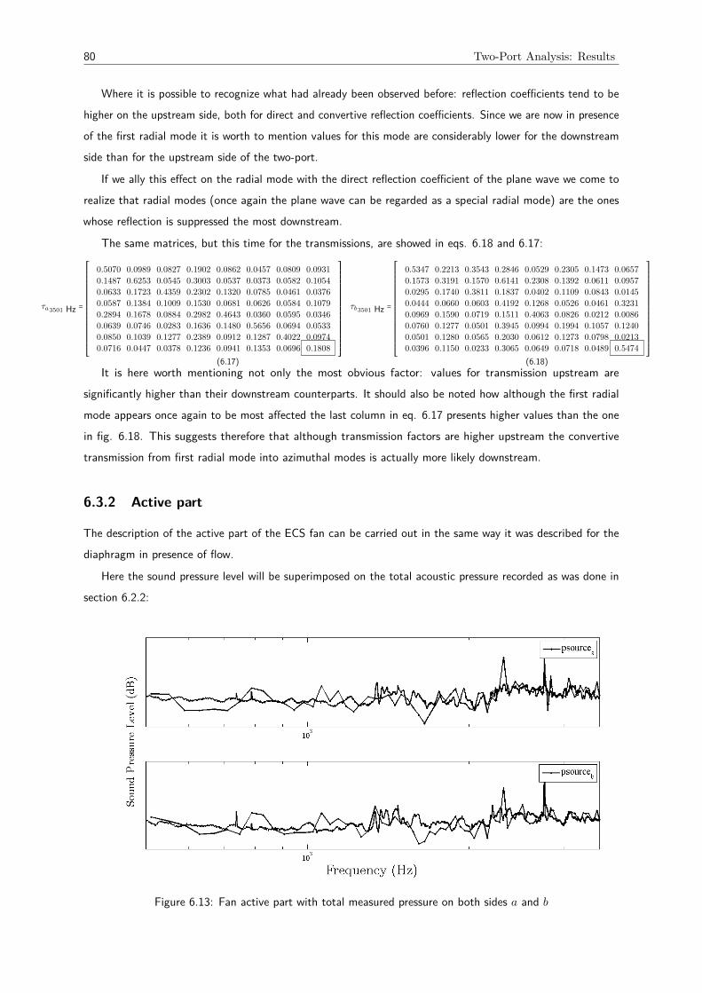
80 Two-Port Analysis: Results
Where it is possible to recognize what had already been observed before: reflection coefficients tend to behigher on the upstream side, both for direct and convertive reflection coefficients. Since we are now in presenceof the first radial mode it is worth to mention values for this mode are considerably lower for the downstreamside than for the upstream side of the two-port.
If we ally this effect on the radial mode with the direct reflection coefficient of the plane wave we come torealize that radial modes (once again the plane wave can be regarded as a special radial mode) are the oneswhose reflection is suppressed the most downstream.
The same matrices, but this time for the transmissions, are showed in eqs. 6.18 and 6.17:
τa3501 Hz =
0.5070 0.0989 0.0827 0.1902 0.0862 0.0457 0.0809 0.09310.1487 0.6253 0.0545 0.3003 0.0537 0.0373 0.0582 0.10540.0633 0.1723 0.4359 0.2302 0.1320 0.0785 0.0461 0.03760.0587 0.1384 0.1009 0.1530 0.0681 0.0626 0.0584 0.10790.2894 0.1678 0.0884 0.2982 0.4643 0.0360 0.0595 0.03460.0639 0.0746 0.0283 0.1636 0.1480 0.5656 0.0694 0.05330.0850 0.1039 0.1277 0.2389 0.0912 0.1287 0.4022 0.09740.0716 0.0447 0.0378 0.1236 0.0941 0.1353 0.0696 0.1808
⎡⎢⎢⎢⎢⎢⎢⎢⎢⎢⎢⎢⎢⎢⎢⎢⎢⎢⎢⎢⎣
⎤⎥⎥⎥⎥⎥⎥⎥⎥⎥⎥⎥⎥⎥⎥⎥⎥⎥⎥⎥⎦
(6.17)
τb3501 Hz =
0.5347 0.2213 0.3543 0.2846 0.0529 0.2305 0.1473 0.06570.1573 0.3191 0.1570 0.6141 0.2308 0.1392 0.0611 0.09570.0295 0.1740 0.3811 0.1837 0.0402 0.1109 0.0843 0.01450.0444 0.0660 0.0603 0.4192 0.1268 0.0526 0.0461 0.32310.0969 0.1590 0.0719 0.1511 0.4063 0.0826 0.0212 0.00860.0760 0.1277 0.0501 0.3945 0.0994 0.1994 0.1057 0.12400.0501 0.1280 0.0565 0.2030 0.0612 0.1273 0.0798 0.02130.0396 0.1150 0.0233 0.3065 0.0649 0.0718 0.0489 0.5474
⎡⎢⎢⎢⎢⎢⎢⎢⎢⎢⎢⎢⎢⎢⎢⎢⎢⎢⎢⎢⎣
⎤⎥⎥⎥⎥⎥⎥⎥⎥⎥⎥⎥⎥⎥⎥⎥⎥⎥⎥⎥⎦
(6.18)It is here worth mentioning not only the most obvious factor: values for transmission upstream are
significantly higher than their downstream counterparts. It should also be noted how although the first radialmode appears once again to be most affected the last column in eq. 6.17 presents higher values than the onein fig. 6.18. This suggests therefore that although transmission factors are higher upstream the convertivetransmission from first radial mode into azimuthal modes is actually more likely downstream.
6.3.2 Active part
The description of the active part of the ECS fan can be carried out in the same way it was described for thediaphragm in presence of flow.
Here the sound pressure level will be superimposed on the total acoustic pressure recorded as was done insection 6.2.2:
Figure 6.13: Fan active part with total measured pressure on both sides a and b
Operating ECS Fan 81
Unlike what had happened for the diaphragm case the source pressure appears to be (as expected) lowerthan the recorded total pressure. This assumption seems more reliable on the upstream side of the ECS fan,with several peaks in the total pressure being matched by increases in the calculated source acoustic pressure.The difference could be related with a preponderance of the plane wave region in the fan generated noise.
6.3.3 Analysis
Analyzing the two-port data for the ECS fan must start with its passive part: note first of all the preponderanceof higher values for reflection in the upstream rather than on the downstream.
This phenomenon, which in the beginning seemed unexpected, can be understood if we consider how thefan induces vorticities and turbulence in the flow downstream from its section, with the flow upstream notpresenting such disturbances. This could therefore mean that flow downstream from an acoustic two-port doesnot really increase reflection, rather suppressing sound due to pressure fluctuations and turbulent effects.
More interesting is to note how transmission effects are higher upstream rather than downstream. Thissuggests that since air is being sucked into the fan sound propagates faster as it accompanies it, in accordanceto what would be expected in the beginning.
However it also interesting to note how convertive reflection coefficients are equally higher for the upstreamside. This in some way corroborates what had been suggested before, if we assume that convertive reflections arenot favored by downstream flow since turbulence actually dissipates acoustic energy thus preventing reflectioncoefficients from achieving higher values.
If the analysis is focused on the first radial mode it is perceptible how this mode’s transmission is stronglysuppressed at the downstream section in comparison with the upstream side. Here it is of course worth torealize what this implies: an axisymmetric mode is hardly transmitted as itself across a two-port source inducingflow with radial velocity [40].
To conclude this topic it should also be noted how convertive transmission terms for the downstreamside are higher than their upstream counterparts. This is in accordance with what was suggested in the lastparagraph since it would be difficult for the radial mode to propagate as itself across the working fan.
Regarding the active part results allow us to observe at which frequencies the fan seems to produce morenoise (namely around the Blade Passing Frequency (BPF) at around 2200 Hz). Also important is to notethat acoustic signatures are similar for both sides, suggesting the acoustic performance of the ECS fan to besymmetrical.
Although results are not lower than total pressure levels it can still be argued (and the same would be validfor the diaphragm situation) that it is possible that at some frequencies the produced sound is being muffled byreflected waves but, once again, this is unlikely and unexpected, since the active part computation is supposedto take this effect into account.


Chapter 7
Conclusions and Future Work
The analysis described in the present thesis allowed for a set of conclusions important not only to develop adeeper knowledge of the mechanics involved but also to set the basis for future related works at VKI given itsinnovative character. Moreover they constituted the first thorough test done on the anechoic termination’sacoustic performance, which provided important results to be taken into account during its future optimization.
To close this thesis a summary of the main conclusions will be outlined, describing the outcome for eachdifferent case and also establishing possible relations between the results for different cases.
Finally the next objectives in this field of research will be here sketched, aiming to provide guidance forfuture works in modal decomposition in duct acoustics
7.1 Terminations
The main conclusions drawn from the terminations tests consist mainly of a series of validations providedfor what had already been suggested by Aguiar [12] and Selamt and Ji [40]. Starting with the horn-shapedinlet located upstream it was possible to identify symmetry patterns related to its shape. Direct reflectioncoefficients were higher than their convertive counterparts and it was shown how reflection is in generalmirrored in the absence of flow. By "mirrored" it’s meant that azimuthal modes with opposite azimuthal modenumbers (m = +N and m = −N) reflect as each other in equal parts, showing the reflection matrix diagonal tobe symmetrical around its center term (plane wave direct reflection coefficient). It was observed that evenwhen values were different their relative values were similar (to each value of the first half of the diagonalcorresponded a closer value in the second in the opposite position). This symmetry effect, described in sec.5.1.2 constitutes the validation of what had already been suggested in the author’s previous work [12].
The anechoic termination proved to yield higher coefficients for most of reflection terms, not inducing lowervalues for convertive reflection coefficients. The basic concept of a set of inverted mufflers proved thereforenot to suppress reflection as expected, being “less anechoic” then the conventional horn-shaped terminationlocated on the upstream end of the duct.
In-duct flow induced convertive reflections at the same time it lowered direct reflection coefficients both forthe anechoic termination and the upstream flow inlet. This effect was first seen as unexpected for the inlet
83
84 Conclusions and Future Work
where the flow had the same direction as the reflected waves but can be seen as a damping in sound pressureby the presence of flow disturbances.
By testing the reflections at different flow speeds it was possible to observe how increasing the flow speedfavors convertive reflection over direct reflection. Both direct and convertive reflection coefficients remainedlower for the inlet even when higher flow speeds were used. This meaning the counter reflection effects displayedby the flow could not be overcome by an increase in the flow speeed.
As referred in sec. 5.3.3 the first radial mode terms decreased as flow assumed higher velocities, retaininglower coefficients for the inlet than for the outlet. These effects were more consistent than those observed forthe azimuthal modes which proved more complex to analyze.
Research has therefore shown that adding in-duct flow does not increase reflection, rather decreasing directreflections (most likely due to turbulence effects) and benefiting convertive reflections both when flow has thesame direction as the emitted or reflected waves.
7.2 Two-Port Analysis
The Two-port analysis performed during IDEALVENT and described in the present thesis constitutes abenchmark in duct acoustic modal decomposition given its innovative and complete approach. To the author’sknowledge there is not any record of similar full spectral modal decomposition tests for two-port sources priorto those performed in the IDEALVENT context.
Starting with the validation case results consolidated the computational approach designed by the authorfor data processing and analysis. It is worth mentioning the accuracy of the transmission coefficients, whoserelative errors remain low for most of the spectrum and are in accordance with those obtained and published bySack [28].
The way how transmission and reflection coefficients deviate from their theoretical values when higher ordermodes are included is evidence of how at cut-on regions the sound field is impossible to describe accuratelywith the current methodology. Acoustic propagation at these thresholds is complex and still mostly unknown.Cut-on frequencies are interpreted as "transition regions" where modes appear to be hard to identify accurately.
Diaphragm tests provided the source for the most diverse data since it constituted the only case when thepresence of flow not only influenced its passive part but actually triggered its active part. Unlike an operatingfan, which in no case possesses only a passive part, the active part of the diaphragm is only triggered when inthe presence of in-duct flow.
For the passive part symmetry was already expected since both sides of the diaphragm are identical. Thissuggests therefore that in the absence of flow reflection and transmission would process in the same way onboth sides. This was effectively observed, and confirmed the theoretical expectations outlined prior to the testcampaigns. Transmission values were shown to be close to 1 for lower frequencies in accordance to what hadalready been suggested before by Sack [28].
The oscillatory behavior displayed by both transmission coefficients could be due to the presence of standingwaves at given frequencies or canceling noise reflections.. The presence of standing patterns in measurementdata from prior tests at VKI’s rig had already been suggested by Aguiar [12] and is still to the day unknown
Two-Port Analysis 85
whether these effects are or not indeed in presence.
When a flow speed of 10 m/s (M=0.0294) was induced reflection coefficients on the upstream side wereseverely increased. Again it was observed how flow having the same direction as reflected waves did notincrease reflection significantly, with the upstream side displaying values for direct reflection terms as highas 0.9. Interesting to note is the fact that the flow did not increase convertive reflections for the upstreamside the same way it increased their downstream counterparts. This therefore allows one to understand howflow across a two-port increases direct reflections upstream and convertive reflections downstream. At thesame time it suppresses direct reflections downstream, probably due to turbulence effects which make directreflections less likely to happen.
One should also note that the presence of flow moving in the reflected wave direction is not necessarily areason why reflection coefficients should increase: sound would move faster in the two-port referential but thatdoes not mean the two-port is more reflective.
Interesting to note this reasoning cannot be extended for transmission factors, where flow proved to providehigher direct transmission coefficients for the upstream side. Convertive terms were higher for the downstreamside for lower frequencies, assuming than lower values when the frequency and higher order modes were included.This disparity suggests therefore some kind of frequency dependent behavior, similar to what had been observedfor transmission factors in the no flow case.
This allows us to conclude then that the presence of flow in a ducted diaphragm increases its upstreamdirect transmission coefficients and lower their downstream counterparts at the same time it favors downstreamconvertive transmissions while upstream convertive transmission coefficients remain low.
Reflection is equally affected by flow, with reflection coefficients being lower downstream (as has alreadybeen observed before) both for direct and convertive reflection coefficients alike.
When the active part is addressed the analysis becomes more complicated: mainly because although theplane wave amplitude can be expected to be higher than the recorded SPL these results have not been validatedyet.
Since values for the calculated active part follow more or less closely the total recorded data it may meanthat some sort of reflective phenomenon is inducing opposite moving waves with opposite phase. This wouldtherefore suppress the original acoustic pressure generated by the source.
Notable is also the fact that the calculated source acoustic levels were shown to be higher upstream thandownstream. This was fully unexpected, specially considering the fact that total recorded pressure was higherdownstream from the diaphragm.
To finish these conclusions the ECS fan case will be addressed last:
Passive part tests showed the plane wave transmission coefficient to be higher upstream. This is under-standable if previous results for the diaphragm passive part are taken into account, and is expected to berelated to sound being carried through the fan by the in-duct flow. Convertive transmission coefficients wereexpected to be high given flow disturbances induced by the fan and convection effects, but as shown in figs.6.17 and 6.18 the convertive transmission terms to have values close to zero.
More important is the pattern displayed by the direct transmission coefficient for the positive first azimuthalmode. This coefficient was significantly higher upstream than downstream. Considering this mode to be a

86 Conclusions and Future Work
spinning mode, whose constant phase surface is helicoidal and similar to that of fig. 3.4 it can be understoodthat a fan spinning induces a flow favorable to the propagation of a first azimuthal mode spinning in the samedirection. Since this only happens for the upstream side and only for one of the azimuthal modes it is likely tobe the cause. This effect had already been suggested by Selamt and Ji [40].
At higher frequencies, when higher order modes were included, convertive transmission terms were equallyhigher for the upstream section, following what had already been referred. The direct transmission coefficient forthe first radial mode proved to be three times higher for the upstream section than its downstream counterpart.
Reflection coefficients were overall lower for both sides when the ECS fan was operating. Although notexempt of the already known lower reflection coefficients for the downstream side, is punctuated by lowerreflection values for positive azimuthal modes on the downstream side. This sort of asymmetry is concordantwith the theory of “favored spinning directions” already suggested in this thesis.
The passive part of an operating ducted fan can therefore be understood as that of a ducted obstacle in thepresence of flow which, by inducing rotating speed in the flow, will favor transmission terms for this directionupstream and suppress its reflection counterparts downstream.
Results for the ECS fan active part were closer to those expected. By observing fig. 6.13 it is possibleto realize how the calculated plane wave amplitude induced by the acoustic source is in general closer to therecorded SPL. This could therefore suggest a preponderance of the plane wave region propagation in the fangenerated noise. An analysis in phase is therefore needed to confirm this theories.
7.3 Future Work
Research work in duct acoustics and modal decomposition at VKI focus on understanding and dealing with theobtained results for active part tests. As suggested by Åbom [22, 25, 26] frequency domain calculations arebased on sample averaging over the data acquired during tests. By not acquiring enough samples (test timesshorter than the required) calculations would not be as accurate as desired, given the preponderance of randomand stochastic errors.
If one the other hand research is directed for a more complete passive part analysis more modes couldbe include, by spanning frequencies after the sixth cut-on. This seems attractive given the fact that at thisfrequency the new mode to propagate has mode numbers m = 1, n = 1 which is, therefore, an hybrid mode. Asso far there are not, to the author’s knowledge, any example of a work as complete as IDEALVENT’s modaldecomposition research, identifying and studying an hybrid mode would constitute yet another benchmark induct acoustics by this project.
On the active part, an analysis not only in amplitude but also in phase is required for the validation of both(diaphragm and fan) active part calculations.

References
[1] A. Earhart, The Fun of It - Random Records of My Own Flying and of Women in Aviation. Brewer,Warner, & Putnam, 1932.
[2] http://boardingarea.com, “History of early commercial aviation at henry ford museum,” March 2014.Quoted from Ford Museum Exibition.
[3] M. K. C. A. Jarrod Mutton, Sam Doolette, “Air pressure control system in passenger aircraft,” TheUniversity of Adelaide.
[4] http://www.britannica.com/, “History of flight,” March 2014.
[5] C. R. Mercer, “Safety with comfort in the passenger cabin,” Lockheed-California Company, 1975.
[6] http://idealvent.eu, “About idealvent,” March 2014.
[7] N. F. R. W. Volker Mellert, Ingo Baumann, “Investigation of noise and vibration impact on aircraft crew,studied in an aircraft simulator,” in The 33rd International Congress and Exposition on Noise Control
Engineering.
[8] N. F. S. B. C. K. V. M. Reinhard Weber, Ingo Baumann, “Effects of noise on the comfort of cabin crewstudied in an aircraft cabin simulator,” Institute of Physiscs, Faculty V, University of Oldenburg, Germany.
[9] Boeing, “737-700/-800 flight crew operations manual,” Tech. Rep. D6-27370-7Q8-SHA, Shangai AirlinesCompany Limited, March 2013.
[10] I. Martínez, “Aircraft environmental control.” available online at http://webserver.dmt.upm.es/.
[11] M. Å. R. Glav, “A general formalism for analyzing acoustic two-port networks,” Journal of Sound and
Vibration, vol. 202, pp. 739–747, September 1997.
[12] J. Aguiar, “Mode scattering in ducted fans,” tech. rep., von Karman Institute for Fluid Dynamics,September 2013.
[13] A. D. Pierce, Acoustics: An Introduction to its Physical Principles and Applications. 1989.
[14] S. Rienstra and A.Hirschberg, An Introduction to Acoustics. December 2013.
[15] S. Dequand, Duct acoustics: from technological applications to the flute. PhD thesis, Eindhoven :Technische Universiteit Eindhoven, 2000.
87
88 References
[16] M. Roger, “Noise in turbomachines,” in VKI Lecture Series, February 2000.
[17] P. O. A. L. Davies, “Practical flow duct acoustics,” Journal of Sound and Vibration, vol. 124, no. 1,pp. 91–115, 1988.
[18] C. L. Morfey, “Sound transmission and generation in ducts with flow,” Journal of Sound and Vibration,vol. 14, no. 1, pp. 37–55, 1971.
[19] R. S. Jeffrey J. Nieter, “Acoustic modal analysis experiment,” Journal of the Acoustical Society of America,vol. 72, pp. 319–326, August 1982.
[20] F. L. V. Gibiat, “Acoustical impedance measurements by the two-microphone-three-calibration (tmtc)method.” October 1990.
[21] J. M. G. S. Oliveira, “Acoustics of annular ducts with impedance walls,” in ICSV16 - The Sixteenth
International Congress on Sound and Vibration, July 2009.
[22] H. B. J. Lavrentjev, M. Åbom, “A measurement method for determining the source data of acoustictwo-port sources,” Journal of Sound and Vibration, vol. 183, no. 3, pp. 517–531, 1995.
[23] H. S. Michito Terao, “In-duct pressure measurements to determine sound generation, characteristicreflection and transmission factors of an air moving device in air-flow,” in Inter-Noise, Newport Beach,
CA, USA, Faculty of Engineering, Kanagawa University, December 1989.
[24] M. Åbom, “Modal decomposition in ducts based on transfer function measurements between microphonepairs,” Journal of Sound and Vibration, vol. 135, no. 1, pp. 95–114, 1989.
[25] M. Åbom, “Measurement of the scattering matrix of acoustical two ports,” Mechanical Systems and
Signal Processing, vol. 5, no. 2, pp. 89–104, 1991.
[26] M. Å. J. Lavrentjev, “Characterization of fluid machines as acoustic multi-port sources,” Journal of Sound
and Vibration, vol. 197, no. 1, pp. 1–16, 1996.
[27] H. B. Andreas Holmberg, Mats Åbom, “Accurate experimental two-port analysis of flow generated soun,”Journal of Sound and Vibration, vol. 330, pp. 6336–6354, 2011.
[28] C. S. K. K. Stefan Sack, Mats Åbom, “Generation and scattering of acoustic modes in ducts with flow,”American Institute of Aeronautics and Astronautics.
[29] M. Å. Stefan Sack, “Experimental characterization of acoustic multi-ports,” in Forum Acusticum, EAA,2014.
[30] H. L. Gareth J. Bennett, Ciarán J. O’Reilly, “Modelling multi-modal sound transmission from point sourcesin ducts with flow using a wave-based method,” in ICSV16- 16th International Congress on Sound and
Vibration, July 2009.
[31] D. F. R. A. F. Seybert, “Experimental determination of acoustic properties using a two-microphonerandom-excitation technique,” Journal of Acoustical Society of America, vol. 61, May 1977.

References 89
[32] J. J. F. M. Å. Ana M. Pedrosa, Francisco D. Denia, “Experimental measurement of acoustic properties bya two source method with simultaneous excitation,” in ICSV18 - 18th International Congress on Sound
and Vibration, July 2011.
[33] M. Å. Antii Hynninem, “Procedure to estimate the in-duct sound power in the high frequency range withnon-plane waves,” in Proceedings of the Internoise /ASME NCAD, August 2012.
[34] J. Y. Chung and D. A. Blaser, “Transfer function method of measuring in-duct acoustic properties. i.theory,” Journal of the Acoustical Society of America, vol. 68, September 1980.
[35] D. A. B. J. Y. Chung, “Transfer function method of measuring in-duct acoustic properties. ii. experiment,”Journal of the Acoustical Society of America, vol. 68, September 1980.
[36] M. Å. Hans Bodén, “Influence of errors on the two-microphone method for measuring acoustic propertiesin ducts,” Journal of the Acoustical Society of America, vol. 79, February 1986.
[37] H. B. Mats Åbom, “Error analysis of two-microphone measurements in duct with flow,” Journal of the
Acoustical Society of America, vol. 83, June 1988.
[38] M. Å. Sabry Allam, Hans Bodén, “Over-determination in acoustic two-port data measurement,” in ICSV13
- Vienna, The Thirteenth Internaitonal Congress on Sound and Vibration, July 2006.
[39] M. Å. A. Holmberg, H. Bodén, “The error suppression of an experimental over-determination of in-ductflow noise sources,” in 16th AIAA/CEAS Aeroacoustics Conference, 2010.
[40] Z. L. J. A. Selamt, “Wave reflection from duct terminations,” Journal of the Acoustical Society of America,vol. 109, April 2001.
[41] F. F. Azzedine Sitel, Jean-Michel Ville, “An experimental facility for measurement of acoustics transmissionmatrix and acoustic power dissipation of duct discontinuity in higher ordermodes propagation conditions,”Acta Acustica united with Acoustica, vol. 89, pp. 586–594, 2003.
[42] J.-M. V. Mohamed Akoum, “Measurement of the reflection matrix of a discontinuity in a duct,” Journal
of the Acoustical Society of America, vol. 103, May 1998.
[43] F. F. Azzedine Sitel, Jean-Michel Ville, “Multiload procedure to measure the acoustic scattering matrix ofa duct discontinuity for higher order mode propagation conditions,” Journal of the Acoustical Society of
America, vol. 120, November 2006.
[44] E. J. Brambley, The acoustics of curved and lined cylindrical ducts with mean flow. PhD thesis, PembrokeCollege, University of Cambridge, August 2007.
[45] V. Zakharov, “Bessel ffunction and their applications to solutions of partial differential equations,” inMath 456 Lecture Notes, 2009.
[46] C. S. S. S. K. Kucukcoskun, J. Aguiar, “Aerodynamic and aeroacoustic installation effects in environmentalcontrol systems,” in ECOMAS, Barcelon, Spain, July 2014.

90 References
[47] R. B. A.F. Smith, N.C. Ovenden, “Flow and geometry induced scattering of high frequency acoustic ductmodes,” Wave Motion, vol. 49, pp. 109–124, August 2011.
[48] R. A. G. Gabard, “A computational mode-matching approach for sound propagation in three-dimensionalducts in flow,” Journal of Sound and Vibration, vol. 315, pp. 1103–1124, March 2008.
[49] D. Greco, “In duct acoustic measurements by mmean of a two-microphone technique,” Master’s thesis,von Karman Insitute for Fluid Dynamics, 2011.
[50] D. L. O’Neal and G. F. Maroney, “National conference on fluid power,” in An anlyisis of four methods for
measuring pump fluid borne noise generation potential, 1977.
[51] M. L. M. M. L. Kathuriya, “Experimental evaluation of the aeroacoustical characteristics of a source ofpulsating gas flow,” Journal of the Acoustical Society of America, vol. 65, pp. 240–248, 1979.
[52] A. D. H.S. Alves, “Noise-con,” in A three-load method for noise source characterization in ducts, 1987.
[53] M. G. Prasad, “A four-load method for evaluation of acoustical source impedance in a duct,” Journal of
Sound and Vibration, vol. 114, pp. 347–356, 1987.
[54] B. S. S. M. J. Crocker, “Error analyss for the four load method,” Journal of Sound and Vibration, vol. 65,pp. 240–248, 1993.
[55] H. Bodén, “The multiple load method for measuring the source characteristics of time-variant sources,”Journal of Sound and Vibration, vol. 148, pp. 437–453, 1991.
[56] G. Golub and W. Kahan, “Calculating the singular values and pseudo-inverse of a matrix,” SIAM Journal
on Numerical Analysis, vol. 2, no. 2, 1965.
[57] W. D. W. De Roeck, “Experimental acoustic identification of flow noise sources in expansion chambers,”tech. rep., Proceedings of ISMA, 2008.
[58] Mathworks.com, “Cross power spectral density - cpsd,” retrieved on June 6, 2014. available athttp://www.mathworks.com/help/signal/ref/cpsd.html.
[59] E. Öngüner, “Aeroacoustics of ducted diaphragms in aircraft environmental control systems: soundproduction and acoustic response,” tech. rep., von Karman Institute for Fluid Dynamics, 2013.
[60] bs EN ISO 5136:1999 acoustics. Determination of sound power radiated into a duct by fans and other
air-moving ddevice. in-duct method, April 2010.