Effect of Turbulence on Wave Propagation in Evaporation Ducts above … · 2017-01-06 · Forum for...

Forum for Electromagnetic Research Methods and ApplicationTechnologies (FERMAT)

Effect of Turbulence on Wave Propagation inEvaporation Ducts above a Rough Sea Surface

Yung-Hsiang Chou and Jean-Fu KiangGraduate Institute of Communication Engineering, NationalTaiwan University, Taipei, Taiwan

(E-mail: [email protected])

Abstract—A proper set of models are carefully selected fromthe literatures to form a wholistic perspective in simulating thewave propagation in evaporation ducts, under a close-to-realisticenvironment. The split-step Fourier (SSF) propagation algorithmis applied to analyze the propagation properties in evaporationducts above a rough sea surface, with turbulence in the ducts.The scattering effect of the rough sea surface is modeled withan effective reflection coefficient, including the Miller-Browncorrection factor for surface roughness. The turbulence effect issimulated with a two-dimensional Kolmogorov power spectrumof refractive index fluctuation, which is derived from the three-dimensional Kolmogorov power spectrum using the Wiener-Khinchin theorem, including the anisotropic effect of the outerscales. The averageM -profile, the outer scales of turbulence, andthe structure constant of the refractive index are categorizedunder different atmospheric conditions. Simulation results arepresented and discussed over all possible atmospheric conditionsto better understand the effect of turbulence on the evaporationducts.

Index Terms—Propagation, split-step Fourier (SSF) algorithm,evaporation duct, rough surface, turbulence, Kolmogorov powerspectrum, refractive index fluctuation.

I. I NTRODUCTION

Measurement of centimeter-wave propagation indicates thatthe difference between the field values inside and above anevaporation duct is much smaller than the prediction usinga simple model [1]. Such difference may be explained asfollows [1], [2]: (1) The height and strength of an evaporationduct can vary with distance, and the wave within an irregularduct is less focused. (2) Roughness of sea surface redirectsalarge portion of wave energy into the space above the duct.(3) Turbulent fluctuations in the atmosphere tends to broadenthe angular spectrum of waves and increase leakage from theduct. Scattering by turbulent atmospheric fluctuations is thestrongest mechanism, at least in certain cases.

For surface-based radars, non-standard tropospheric refrac-tion such as ducting may result in an anomalous propagationcondition, bending the radar ray from the anticipated direction[3]. Anomalous propagation echoes have been observed in fairweather conditions; more frequently in summer than in winter,more frequently in tropical areas than in the middle and higherlatitudes [4].

Ducting may seriously affect radio communications links,extend the radar range of a target at or near the sea surface

This work was sponsored by the National Science Council, Taiwan, ROC,under contract NSC 100-2221-E-002-232.

to be considerably longer than if in the free-space [5]. Evap-oration duct is a surface duct appearing over water bodies,featuring rapid decrease of humidity with height. It is the mostcommon type of anomalous propagation over oceans and otherlarge bodies of water. The worldwide mean of the evaporationduct height (EDH) is about 10 m [6], sometimes reaches30 mor 40 m [7]. The EDH increases during the summer monthsand during the daytime [8]. With the evaporation ducts soclose to the sea surface, the latter has very strong effects onthe signal propagating in the ducts.

The effects of duct on communications links have beenstudied [9], [10]. Possible effects of tropospheric ductingon short-distance wireless communications have also beenreported [11]. The effects of evaporation and surface-basedducts on microwave path loss have been studied [12]. In [13],the path-loss variations are compared with the monthly andseasonal mean parameters of surface ducts, based on a two-year statistical study of surface-duct formation at Istanbul, overa WCDMA-FDD downlink band [14]. Ducts frequently appearin the coastal areas where the horizontal change of refractivitycan not be neglected. In [12], a comparison is made betweena range independent surface-based duct and a mixed land-seapath, using twoM -profiles.

Propagation experiments have been conducted in theMediterranean and the North Sea areas [15], [16]. The receivedsignal is stronger than expected, which is a sign that theevaporation ducting effect may dominate over the gaseousabsorption in the 10-20 GHz band. Measurements at 18 GHzhave been conducted to demonstrate the enhancement on radarcoverage and range detection due to an evaporation duct [17],[7]. While the predictions and the measurements seem to agreereasonably well, the predictions tend to underestimate thepathloss when the duct heights are low. Although the predictionmodel incorporates the Kirchhoff theory to account for thescattering from a rough sea surface, it does not consider thescattering due to the turbulent fluctuations in the refractiveindex [18].

An evaporation duct can significantly increase the signalstrength near the sea surface for over-the-horizon paths, atfrequencies above 3 GHz. As the frequency is higher than10 GHz, the signal strength is reduced by scattering fromthe wind-driven rough sea surface. Such signal reductionis more obvious under strong ducting conditions and largesea-wave heights [19]. In [19], an MLAYER propagationmodel, including the Miller-Brown reflection reduction factor(RRF), is used to compare with the measurements. In all the

1


cases studied in [19], the model including rough sea surfaceprovides a closer match with the measurement results thanthe model with smooth sea surface, but the former model stillunderestimates the path loss by 3 to 12 dB. The refractive-index fluctuation may partly account for this underestimate.

The effects of air turbulence have been analyzed by applyinga small-perturbation method to a mode-based model [18], orapplying a phase-screen method to a split-step Fourier (SSF)model [20], [21]. Different models have been compared ona series of over-water measurements, in a nearly standard at-mosphere [21]. The model including the turbulence scatteringperforms better than the other models, in the sense of matchingwith the measured data. At higher frequencies, the effects ofturbulent scattering become even stronger.

In [22], two approaches are proposed to model the surface-layer turbulence effects in a marine environment at microwavefrequencies. One is the SSF method with phase screen, theother is a direct computation of the log-amplitude varianceofsignals. Their results are compared with the observation, andthe effect of the power-law constant on the first approach isalso discussed.

In [23], the phase screen method is adopted in the split-step Fourier algorithm to simulate the turbulence effect inanevaporation duct. It is assumed that the atmosphere is undertheneutral condition, the turbulence follows the one-dimensionalKolmogorov spectrum, the structure constant and the outerscale are constant, and the sea surface is smooth [23]. Thesimulation results show that the refractive-index fluctuationleads to energy leakage away from the duct, causing anadditional path loss within the duct. The height distribution ofradiated power becomes more uniform than that without thefluctuations. The power leakage along the evaporation duct isnot uniform. It is also observed that the received power levelabove the duct fluctuates more significantly than within theduct when the refractive-index fluctuation is considered.

Diffraction by a relatively smooth sea surface can be de-scribed by introducing an effective reflection coefficient [24]into the boundary condition, which is the flat-surface Fresnelreflection coefficient multiplied by a roughness reductionfactor (RRF). In general, a rough sea surface tends to destroythe trapping property of the duct structure and changes thepath-loss pattern. In [25], the effects of wind direction onelectromagnetic waves propagation over rough sea surface arestudied by mixing two approaches applicable at large andsmall roughness, respectively.

The interaction among sea waves is nonlinear, renderingthe sea-surface statistics different from a Gaussian distribution[26]. It has been demonstrated that the shadowing effectprevails over the non-Gaussian statistics of a sea surface,especially in the presence of an evaporation duct at thecentimeter wavelength [27].

The wave equation can be reduced to a parabolic equation(PE), which is then solved using numerical techniques like thesplit-step Fourier (SSF) algorithm [28], finite difference(FD)algorithm [24], and finite element (FE) algorithm [29]. TheFD and FE algorithms are more flexible to implement variousboundary conditions. The SSF algorithm is numerically stableand allows a larger step size to compute the field distribution

at long distances.Reasonable agreement between measured and predicted

field strength using the PE model has been achieved in atropical maritime environment [30]. It is shown that the PEmodel gives a good estimation of path factor over a widerange of frequencies (X, Ka and W bands) and a variety ofatmospheric conditions [31]. The difficulties in predicting thefield strength of maritime links and the importance of higherM -inversion can be found in [32].

Numerical analysis indicates that the microwave inside anevaporation duct suffers an additional path loss in the presenceof turbulence [33]. Monte-Carlo method has been used tostudy the scattering properties of scalar waves in randomlyfluctuating slabs with an exponential spatial correlation,and ithas also been extended to random media with non-exponentialspatial correlation and background inhomogeneity [34], [35].

The prediction accuracy of the PE models is constrainedby the environmental parameters, especially in littoral envi-ronments [12], [36]. Three-dimensional PE models have beendeveloped [37], [38], covering the sea-surface roughness effect[25] and the evaporation ducts [39]. PE-based time-dependentpropagation model has also been explored [40].

Although many of the key factors on evaporation ducts,like refractive-index profile, rough surface, wind profile,tur-bulence, have been analyzed or modeled; few literatures, ifnotnone, integrate all the relevant factors together to analyze orsimulate wave propagation in evaporation ducts under a close-to-realistic environment. In this work, we carefully reviewmany existing models about these factors, and choose a properset of models to simulate the wave propagation in evaporationducts, under all possible atmospheric conditions. During thereview process, it is observed that the wind profile, which canbe categorized with a stability index of the atmosphere, seemsto be a common factor behind all these models. As a result, thiswork provides a wholistic perspective on the subject issues.The simulation results may also help reveal more values ofthe existing models and inspire more ideas from the readers.

In this work, the SSF algorithm is used to simulate wavepropagation over long distances. The Miller-Brown [42] for-mula of RRF is adopted to model the rough sea surface.Monte-Carlo method is used to generate profiles of refractive-index fluctuations to simulate the turbulence in the atmosphere.The relevant models are described in Section II, the properranges of parameters in these models are estimated in SectionIII, the simulation of practical evaporation ducts is presentedand discussed in Section IV, followed by the conclusion.

II. CONSTRUCTION OFMODELS

A. Propagation Model

The parabolic equation is a paraxial approximation to theHelmholtz wave equation, under the assumption that the elec-tromagnetic wave predominantly propagates in the horizon-tal direction, x. The two-dimensional narrow-angle forward-scattering scalar form of the parabolic equation takes the form[28]

∂u(x, z)

∂x≃ −j

{

k

2[m2(x, z)− 1] +

1

2k

∂2

∂z2

}

u(x, z) (1)

2


wherek is the wavenumber in the background medium,m =1+M×10−6, with the modified refractivity,M , related to therefractivity,N , asM = N +0.157z. Eqn. (1) is very accuratewith the propagation angle about the horizontal direction fallswithin |θ| < 15◦ [24].

The split-step solution to (1) can be expressed as [28]

u(x+∆x, z) = e−j(k/2)(m2−1)∆x

F−1{

ej(p2/2k)∆xF{u(x, z)}

}

(2)

where p = k sin θ is the vertical wavenumber. The solutionu(x, z) and its spectrumU(x, p) are related by the FouriertransformF{·} and its inverseF−1{·} as

F{u(x, z)} =1√2π

∫

∞

−∞

u(x, z)ejpzdz

F−1{U(x, p)} =1√2π

∫

∞

−∞

U(x, p)e−jpzdp

To represent wave propagation over a perfect electric con-ductor (PEC) surface, either a Dirichlet (horizontal polariza-tion) or a Neumann (vertical polarization) boundary conditionis imposed. To represent wave propagation over a smoothimpedance surface, the boundary condition can be specifiedas [43]

(

∂

∂z+ αh,v

)

u(x, z) = 0 (3)

with

αh,v = −jk sinχ1−Reff

1 +Reff(4)

whereχ = 90◦ − θi is the grazing angle,Reff is the Fresnel’sreflection coefficient,Rh

F or RvF , with

RhF =

sinχ−√

ǫsr − cos2 χ

sinχ+√

ǫsr − cos2 χ(5)

RvF =

ǫsr sinχ−√

ǫsr − cos2 χ

ǫsr sinχ+√

ǫsr − cos2 χ(6)

for the horizontal and the vertical polarization, respectively;

ǫsr = ǫs/ǫ0 = ǫr − j60σλ

is the effective dielectric coefficient of the sea sea surface, σand ǫr are the conductivity and relative permittivity, respec-tively, of the sea water [44].

The boundary condition can be incorporated into the stan-dard split-step PE approach through the use of mixed Fouriertransform [28], [43]. The path loss (PL) is defined as [24]

PL = 20 log

(

4π√x

λ3/2|u(x, z)|

)

, dB (7)

whereλ is the wavelength of the wave, andx is the propaga-tion range.

B. Effective Reflection Coefficient of Rough Sea Surface

The roughness effect can be incorporated by multiplying theFresnel’s reflection coefficient,RF , by a roughness reductionfactor (RRF),ρMB, to obtain an effective reflection coefficient[24]

Reff = ρMBRF

where

ρMB = e−γ2/2I0(

γ2/2)

(8)

is the Miller-Brown roughness reduction factor [42],I0(α) isthe zeroth-order modified Bessel function of the first kind. Therelevant parameters have the form

γ = 2kσh sinχ

σh = 5.1× 10−3U210 (9)

whereσh is the standard deviation of the sea wave,k is thewavenumber of the signal, andU10 is the reference wind speedat 10 m above the sea level. Note that the RRF in (8) affectsthe magnitude of the complex Fresnel reflection coefficient,but does not account for the shadowing effect [45] or thegeometry of the sea surface [25]. At near grazing incidence,the shadowing effect may have stronger effect on the wavepropagation [45].

C. Refractive Index Fluctuation

The total refractive-index is expressed as

n(x, z) = n(z) + nf (x, z) (10)

wheren(z) is the average refractive index, which is a functionof altitude, andnf (x, z) is the fluctuation of the refractive-index. The turbulence is approximated as frozen [46] duringthe period the electromagnetic wave propagates from thetransmitting antenna to the receiving one. By applying theMonte-Carlo technique, one sample profile of refractive-indexfluctuation, of a two-dimensional turbulence, can be realizedas [34], [41]

n(s)f (x, z) =

∞∑

p=1

∞∑

q=1

a(s)pq sin(ζxpx+ ζzqz) + b(s)pq cos(ζxpx+ ζzqz) (11)

wheres indicates thesth realization,ζxp and ζzq are thepthandqth discretized wavenumber, respectively,apq andbpq arerandom numbers with varianceσ2

pq, which can be expressedas

σ2pq = 4∆ζxp∆ζzqFn(ζxp, ζzq) (12)

whereFn(ζx, ζz) is the two-dimensional power spectral den-sity of the refractive-index fluctuation.

The three-dimensional power spectral density of refractive-index in an isotropic Kolmogorov turbulence is [47]

ΦKn (ζx, ζy, ζz) =

0.033C2n

(ζ2x + ζ2y + ζ2z + 1/L20)

11/6(13)

WhereL0 is the outer scale, andC2n is the structure constant.

By the Wiener-Khinchin theorem [48], the two-dimensional

3


power spectral density, independent of they coordinate, canbe derived as

FKn (ζx, ζz) =

∫

∞

−∞

ΦKn (ζx, ζy, ζz)dζy

=0.0555C2

n

(ζ2x + ζ2z + 1/L20)

4/3(14)

which is an isotropic Kolmogorov turbulence. Next, followthe same approach as in [47] to modify (14) to be a two-dimensional anisotropic Kolmogorov spectrum

FKn (ζx, ζz) =

0.0555C2n(L0hL0v)

4/3

(ζ2xL20h + ζ2zL

20v + 1)4/3

(15)

whereL0v andL0h are the outer scales in the vertical and thehorizontal directions, respectively.

III. E STIMATION OF PARAMETERS

A. Average Modified Refractivity

The PJ model is adopted to generate profiles of modifiedrefractivity under different atmospheric conditions as [49], [50]

M(z) =M(0) +z

8−

zd

ln4(1 + z/z0)

(

1 +√

1− 16z/Lmo

)2

8/√

1− 16zd/Lmo

,

z/Lmo ≤ 0

zdln(1 + z/z0) + 5z/Lmo

8(1 + 5zd/Lmo),

z/Lmo ≥ 0

(16)

whereLmo is the Monin-Obukhov length,zd (in m) is the ductheight, andz0 (in m) is the roughness length of the surface.Typically, z0 increases with the wind speed, ranging from10−4 m on a calm open sea to10−3 m in coastal areas withoff-sea wind [50]. The value ofz/Lmo is used to categorizethe atmospheric condition: Stable ifz/Lmo > 0, unstable ifz/Lmo < 0, and neutral ifz/Lmo = 0.

B. Monin-Obukhov Length

The Monin-Obukhov length is essentially dependent uponthe heat flux and the friction velocity, which can be treatedas independent of height within the surface layer. The gen-eral characteristics of the atmosphere can be categorized interms ofz/Lmo as follows [50]: WhenLmo is negative withvery small magnitude (z/Lmo becomes negative with largemagnitude ), the heat convection dominates. WhenLmo isnegative with large magnitude (z/Lmo becomes negative withsmall magnitude), the mechanical turbulence dominates. Whenz/Lmo = 0, only mechanical turbulence contributes. Whenz/Lmo is a small positive number, the mechanical turbulenceis slightly damped by the temperature stratification. Whenz/Lmo is a large positive number, the mechanical turbulenceis severely reduced by the temperature stratification. Thenumber |z/Lmo| describes the relative significance betweenheat convection and mechanical turbulence during the daytime,and to what extent the stratification suppresses the mechanicalturbulence during the night time, respectively.

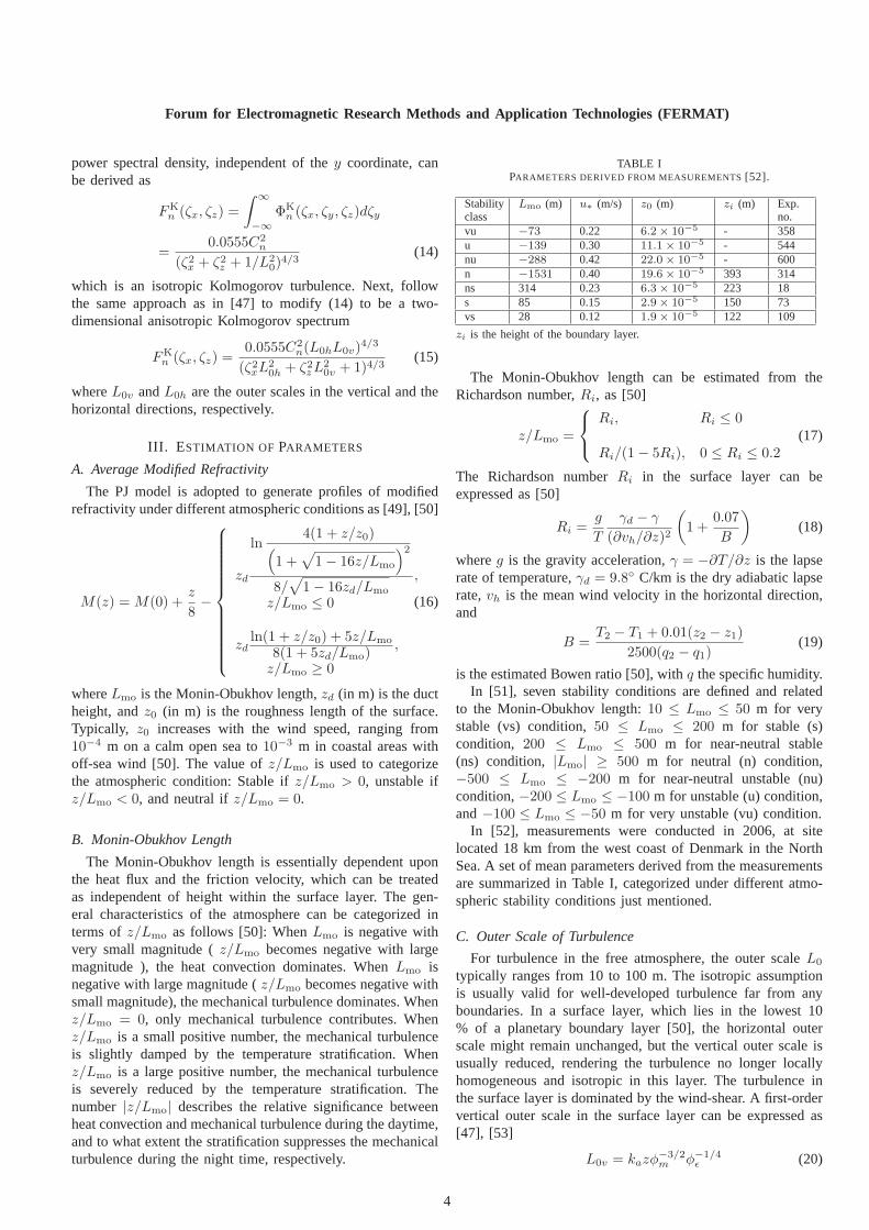
TABLE IPARAMETERS DERIVED FROM MEASUREMENTS[52].

Stabilityclass

Lmo (m) u∗ (m/s) z0 (m) zi (m) Exp.no.

vu −73 0.22 6.2× 10−5 - 358u −139 0.30 11.1× 10−5 - 544nu −288 0.42 22.0× 10−5 - 600n −1531 0.40 19.6× 10−5 393 314ns 314 0.23 6.3× 10−5 223 18s 85 0.15 2.9× 10−5 150 73vs 28 0.12 1.9× 10−5 122 109

zi is the height of the boundary layer.

The Monin-Obukhov length can be estimated from theRichardson number,Ri, as [50]

z/Lmo =

Ri, Ri ≤ 0

Ri/(1− 5Ri), 0 ≤ Ri ≤ 0.2(17)

The Richardson numberRi in the surface layer can beexpressed as [50]

Ri =g

T

γd − γ

(∂vh/∂z)2

(

1 +0.07

B

)

(18)

whereg is the gravity acceleration,γ = −∂T/∂z is the lapserate of temperature,γd = 9.8◦ C/km is the dry adiabatic lapserate,vh is the mean wind velocity in the horizontal direction,and

B =T2 − T1 + 0.01(z2 − z1)

2500(q2 − q1)(19)

is the estimated Bowen ratio [50], withq the specific humidity.In [51], seven stability conditions are defined and related

to the Monin-Obukhov length:10 ≤ Lmo ≤ 50 m for verystable (vs) condition,50 ≤ Lmo ≤ 200 m for stable (s)condition, 200 ≤ Lmo ≤ 500 m for near-neutral stable(ns) condition, |Lmo| ≥ 500 m for neutral (n) condition,−500 ≤ Lmo ≤ −200 m for near-neutral unstable (nu)condition,−200 ≤ Lmo ≤ −100 m for unstable (u) condition,and−100 ≤ Lmo ≤ −50 m for very unstable (vu) condition.

In [52], measurements were conducted in 2006, at sitelocated 18 km from the west coast of Denmark in the NorthSea. A set of mean parameters derived from the measurementsare summarized in Table I, categorized under different atmo-spheric stability conditions just mentioned.

C. Outer Scale of Turbulence

For turbulence in the free atmosphere, the outer scaleL0

typically ranges from 10 to 100 m. The isotropic assumptionis usually valid for well-developed turbulence far from anyboundaries. In a surface layer, which lies in the lowest 10% of a planetary boundary layer [50], the horizontal outerscale might remain unchanged, but the vertical outer scale isusually reduced, rendering the turbulence no longer locallyhomogeneous and isotropic in this layer. The turbulence inthe surface layer is dominated by the wind-shear. A first-ordervertical outer scale in the surface layer can be expressed as[47], [53]

L0v = kazφ−3/2m φ−1/4

ǫ (20)

4


whereka is the von Karman’s constant,φm is the normalizedwind shear, andφǫ is the normalized turbulent kinetic energydissipation rate. The von Karman’s constant is conventionallytaken to be 0.4. Its value measured in the wind tunnel andthe atmosphere ranges from 0.35 to 0.43 [50], [54]. Thenormalized wind shear is defined as [50]

φm =kaz

u∗

∂u

∂z(21)

and the normalized turbulent kinetic energy dissipation rate isdefined as [50]

φǫ =kaz

u3∗

ǫ (22)

whereu is the wind velocity,u∗ is the friction velocity, andǫ isthe dissipation rate. The profiles ofφm andφǫ under differentconditions are [50]

φm =

(1− 16z/Lmo)−1/4

, −2 ≤ z/Lmo ≤ 0

(1− 15z/Lmo)−1/3

, z/Lmo < −2

1 + 5z/Lmo, z/Lmo > 0

φǫ =

1− z/Lmo, z/Lmo ≤ 0

[

1 + 2.5 (z/Lmo)0.6

]3/2

, z/Lmo > 0

(23)

The vertical outer scale of the turbulence in a surface layer,under different atmospheric conditions, are derived by substi-tuting (23) into (20):

L0v =

kaz (1− z/Lmo)−1/4

(1− 16z/Lmo)3/8 , −2 ≤ z/Lmo ≤ 0

kaz (1− z/Lmo)−1/4

(1− 15z/Lmo)1/2 , z/Lmo < −2

kaz(1 + 5z/Lmo)−3/2

[

1 + 2.5(z/Lmo)0.6

]3/8 , z/Lmo > 0

(24)

whereka = 0.4 [47].

D. Anisotropy of Turbulence

Turbulence at large scales is usually anisotropic, withconsiderably different outer scales in the horizontal and thevertical directions. The anisotropy and the length of the outerscale is dependent upon the atmospheric stability [55], [56].The anisotropy of the outer scale becomes more obviouswith stronger temperature inversion and weaker wind, whichcorrespond to a higher Richardson number and a more stablystratified atmosphere. In such a weather condition with stableair, the mechanical turbulence is strongly damped by strati-fication, hence the vertical outer scale become much smallerthan the horizontal one. In [55], it is also confirmed that if theturbulent energy is mainly generated from mechanical origin,the eddies are small, the outer scale length tends to decreasewith increased wind speed, and vice versa, which is muchmore obvious in the horizontal scales.

The anisotropy has no significant influence on power fluc-tuation, but the angle-of-arrival [55]. In [50], the ratio of thehorizontal to the vertical integral scale (similar to the outerscale) of wind fluctuations has been estimated. It is shownthat with an increasing positive Richardson number, a muchlarger outer scale is expected in the horizontal direction.Underneutral condition (Ri ≃ 0), the horizontal and the verticalouter scales are similar. In an unstable air (Ri < 0), eddiestend to be vertically elongated. In [56], it is empirically foundthat L0h/L0v ≃ (30 ± 10)Ri under stable condition. Thewide range of variation might be attributed to the fact thatthe anisotropy does not solely depend onRi.

The anisotropy of the turbulence can be related to thestability of atmosphere as [57]

az =10 (1− z/Lmo)

0.5− z/Lmo, z/Lmo < 0.5 (25)

whereaz = 4πL0h/L0v is the decay constant of the verticalcoherence of wind components [50], [58]. Eqn. (25) implies

L0h/L0v =10(1− z/Lmo)

4π(0.5− z/Lmo), z/Lmo < 0.5 (26)

E. Structure Constant

Turbulence is likely to become strong ( structure constant,C2

n, becomes large ) near the earth surface and in the clouds[59]. The magnitude ofC2

n generally increases with increasingwavelength, because the contribution of moisture toC2

n signif-icantly increases with increasing wavelength. The magnitudeof C2

n in near-millimeter-wave band can be larger than that inthe infrared by orders of magnitude. The magnitude ofC2

n inthe visible and the infrared bands near the ground falls in therange from10−16 to 10−12 m−2/3 [60].

The structure constant of the refractive-index fluctuationinthe planetary boundary layer can be expressed as [47], [53]

C2n = a2L

4/30v

(

∂〈n〉∂z

)2

(27)

wherea2 lies between 1.5 and 3.5 [47], [50]. Substituting (16)into (27), we have

C2n = 2.8L

4/30v × 10−12

[

0.032 +zd√

1− 16zd/Lmo8

(

16/Lmo

1− 16z/Lmo +√

1− 16z/Lmo

+1

z + z0

)]2

,

z/Lmo ≤ 0

[

0.032 +zd [5/Lmo + 1/(z + z0)]

8(1 + 5zd/Lmo)

]2

,

z/Lmo ≥ 0

(28)

wherea2 = 2.8 andka = 0.4 are chosen [47].In the experiments considered in [61], the moisture fluctu-

ation plays a dominant role, as compared to temperature, indetermining the microwaveC2

n; and significantly affects theacoustic and opticalC2

n values, since the near-surface turbu-lence leads to relatively large moisture fluctuations. The over-land experiment shows a larger diurnal variation, while the

5


moisture fluctuation does not play a dominant role [61]. Thetemperature makes a comparable contribution to microwaveC2

n near the surface, particularly in the afternoon. For theacoustic and optical waves, theC2

n primarily depends on thetemperature fluctuations.

F. Surface Roughness

The wind profile in the surface layer can be described as[50], [51]

u =

u∗ka

(

lnz

z0− ψm

)

, z/Lmo ≤ 0

u∗ka

[

lnz

z0− ψm

(

1− z

2zi

)]

, z/Lmo ≥ 0

(29)

wherezi is the height of boundary layer, andψm is calculatedas [50]

ψm =

∫ z/Lmo

z0/Lmo

(1− φm)d(z/Lmo)

z/Lmo(30)

By substituting (23) into (30) and ignoringz0/Lmo, (30) canbe expressed as

ψm =

−5z/Lmo, z/Lmo > 0

ln{

[

(1 + x21)/2]

[(1 + x1)/2]2}

−2 tan−1 x1 + π/2,0 ≥ z/Lmo ≥ −2

(3/2) ln[

(x22 + x2 + 1)/3]

−√3 tan−1

[

(2x2 + 1)/√3]

+ π/√3,

z/Lmo < −2

(31)

wherex1 = (1− 16z/Lmo)1/4 andx2 = (1− 15z/Lmo)

1/3.A smooth sea surface can be approximated as a perfectly

conducting surface, and a rough sea surface can be modeledwith the Miller-Brown roughness reduction factor. The windspeed at 10 m height,U10, is used to represent the on-shorewind under a near-neutral atmospheric condition.

G. Evaporation Duct Height

Duct height variation with wind speed has been reported in[62]. The coastal areas are especially rich in super-refractivelayers and ducts that affect microwave propagation [63]. In[64], cumulative distribution functions of duct height arederived in three locations. A larger variation in duct height isobserved around the Lucinda data than in the Coral Sea. Whensea breezes are the dominant wind flow, duct heights can behighly variable over a 24 hour cycle. The ducting events inthe Coral Sea occurred under stable weather conditions, withlittle variation in wind speed; while the ducting events in theWestern Pacific Ocean shows the greatest variation in ductheight because of the highly variable weather.

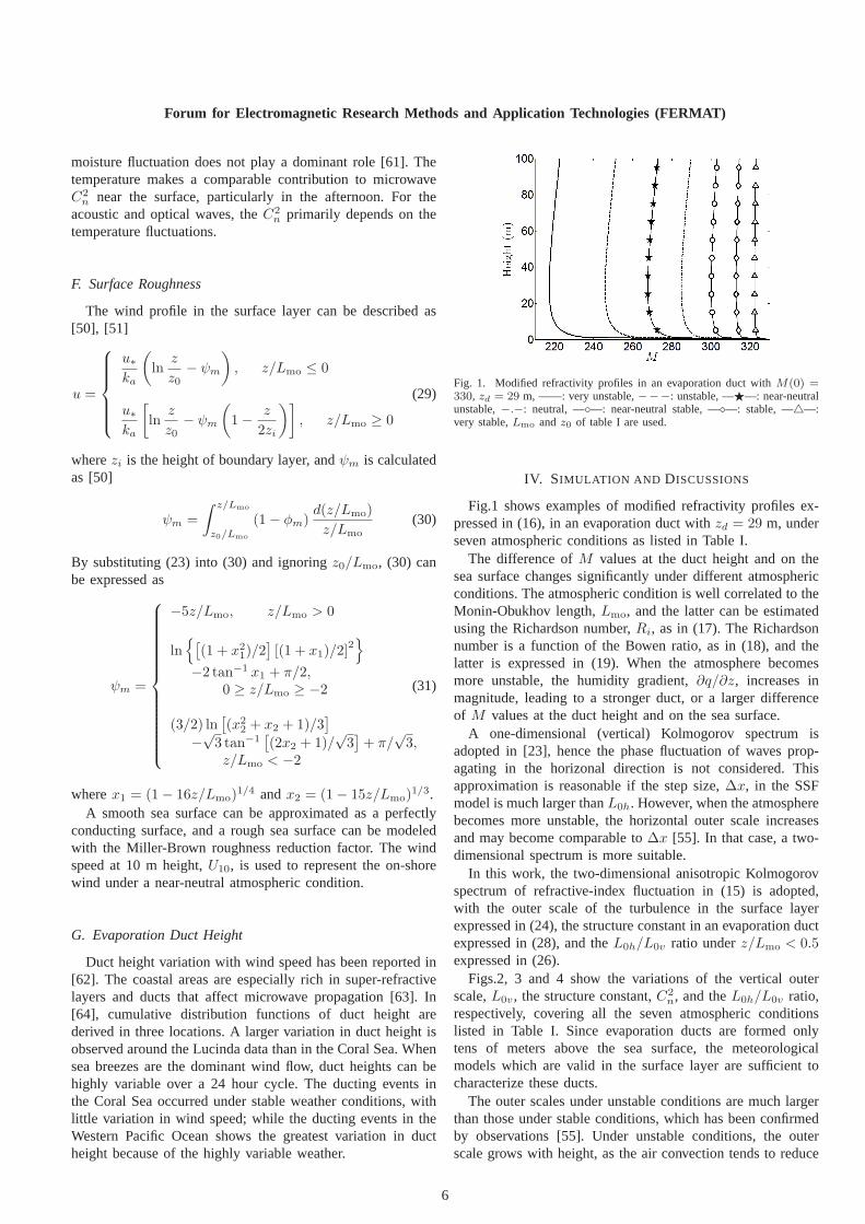
Fig. 1. Modified refractivity profiles in an evaporation ductwith M(0) =330, zd = 29 m, ——: very unstable,−−−: unstable, —⋆—: near-neutralunstable,−.−: neutral, —◦—: near-neutral stable, —⋄—: stable, —△—:very stable,Lmo andz0 of table I are used.

IV. SIMULATION AND DISCUSSIONS

Fig.1 shows examples of modified refractivity profiles ex-pressed in (16), in an evaporation duct withzd = 29 m, underseven atmospheric conditions as listed in Table I.

The difference ofM values at the duct height and on thesea surface changes significantly under different atmosphericconditions. The atmospheric condition is well correlated to theMonin-Obukhov length,Lmo, and the latter can be estimatedusing the Richardson number,Ri, as in (17). The Richardsonnumber is a function of the Bowen ratio, as in (18), and thelatter is expressed in (19). When the atmosphere becomesmore unstable, the humidity gradient,∂q/∂z, increases inmagnitude, leading to a stronger duct, or a larger differenceof M values at the duct height and on the sea surface.

A one-dimensional (vertical) Kolmogorov spectrum isadopted in [23], hence the phase fluctuation of waves prop-agating in the horizonal direction is not considered. Thisapproximation is reasonable if the step size,∆x, in the SSFmodel is much larger thanL0h. However, when the atmospherebecomes more unstable, the horizontal outer scale increasesand may become comparable to∆x [55]. In that case, a two-dimensional spectrum is more suitable.

In this work, the two-dimensional anisotropic Kolmogorovspectrum of refractive-index fluctuation in (15) is adopted,with the outer scale of the turbulence in the surface layerexpressed in (24), the structure constant in an evaporationductexpressed in (28), and theL0h/L0v ratio underz/Lmo < 0.5expressed in (26).

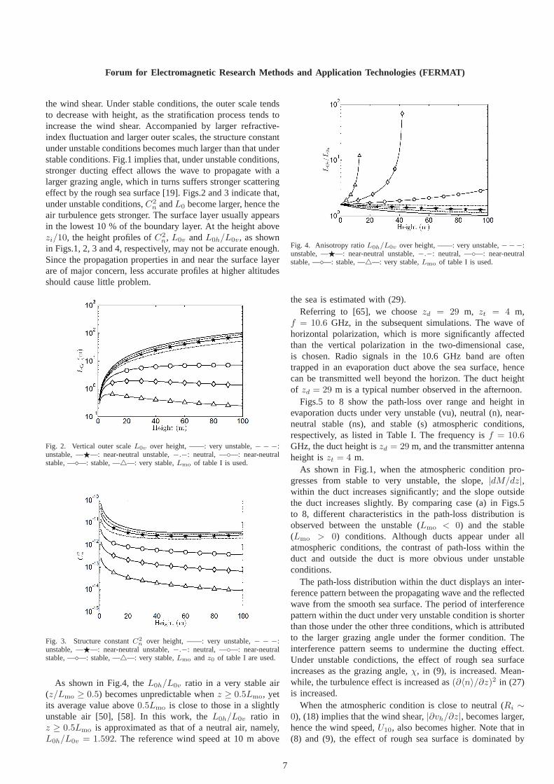
Figs.2, 3 and 4 show the variations of the vertical outerscale,L0v, the structure constant,C2

n, and theL0h/L0v ratio,respectively, covering all the seven atmospheric conditionslisted in Table I. Since evaporation ducts are formed onlytens of meters above the sea surface, the meteorologicalmodels which are valid in the surface layer are sufficient tocharacterize these ducts.

The outer scales under unstable conditions are much largerthan those under stable conditions, which has been confirmedby observations [55]. Under unstable conditions, the outerscale grows with height, as the air convection tends to reduce

6


the wind shear. Under stable conditions, the outer scale tendsto decrease with height, as the stratification process tendstoincrease the wind shear. Accompanied by larger refractive-index fluctuation and larger outer scales, the structure constantunder unstable conditions becomes much larger than that understable conditions. Fig.1 implies that, under unstable conditions,stronger ducting effect allows the wave to propagate with alarger grazing angle, which in turns suffers stronger scatteringeffect by the rough sea surface [19]. Figs.2 and 3 indicate that,under unstable conditions,C2

n andL0 become larger, hence theair turbulence gets stronger. The surface layer usually appearsin the lowest 10 % of the boundary layer. At the height abovezi/10, the height profiles ofC2

n, L0v andL0h/L0v, as shownin Figs.1, 2, 3 and 4, respectively, may not be accurate enough.Since the propagation properties in and near the surface layerare of major concern, less accurate profiles at higher altitudesshould cause little problem.

Fig. 2. Vertical outer scaleL0v over height, ——: very unstable,− − −:unstable, —⋆—: near-neutral unstable,−.−: neutral, —◦—: near-neutralstable, —⋄—: stable, —△—: very stable,Lmo of table I is used.

Fig. 3. Structure constantC2n over height, ——: very unstable,− − −:

unstable, —⋆—: near-neutral unstable,−.−: neutral, —◦—: near-neutralstable, —⋄—: stable, —△—: very stable,Lmo andz0 of table I are used.

As shown in Fig.4, theL0h/L0v ratio in a very stable air(z/Lmo ≥ 0.5) becomes unpredictable whenz ≥ 0.5Lmo, yetits average value above0.5Lmo is close to those in a slightlyunstable air [50], [58]. In this work, theL0h/L0v ratio inz ≥ 0.5Lmo is approximated as that of a neutral air, namely,L0h/L0v = 1.592. The reference wind speed at 10 m above

Fig. 4. Anisotropy ratioL0h/L0v over height, ——: very unstable,−−−:unstable, —⋆—: near-neutral unstable,−.−: neutral, —◦—: near-neutralstable, —⋄—: stable, —△—: very stable,Lmo of table I is used.

the sea is estimated with (29).Referring to [65], we choosezd = 29 m, zt = 4 m,

f = 10.6 GHz, in the subsequent simulations. The wave ofhorizontal polarization, which is more significantly affectedthan the vertical polarization in the two-dimensional case,is chosen. Radio signals in the 10.6 GHz band are oftentrapped in an evaporation duct above the sea surface, hencecan be transmitted well beyond the horizon. The duct heightof zd = 29 m is a typical number observed in the afternoon.

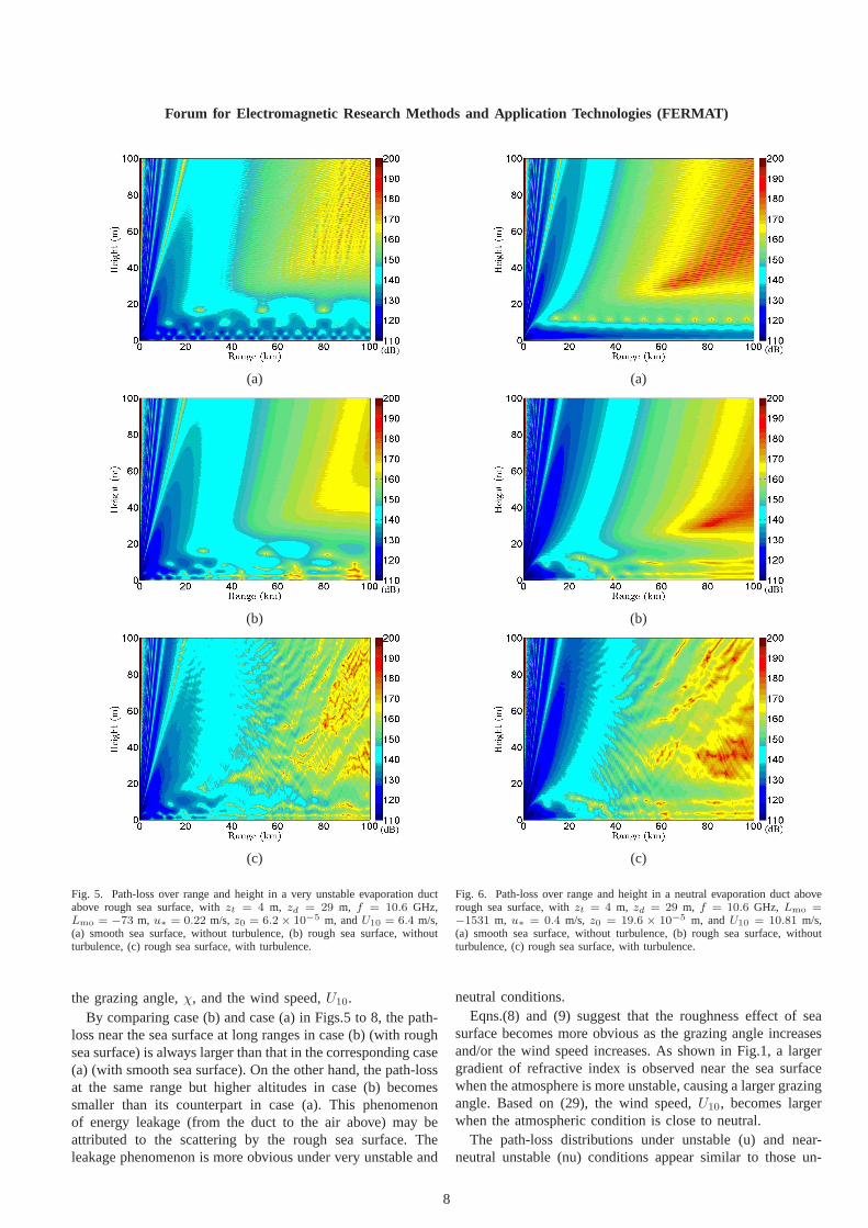
Figs.5 to 8 show the path-loss over range and height inevaporation ducts under very unstable (vu), neutral (n), near-neutral stable (ns), and stable (s) atmospheric conditions,respectively, as listed in Table I. The frequency isf = 10.6GHz, the duct height iszd = 29 m, and the transmitter antennaheight iszt = 4 m.

As shown in Fig.1, when the atmospheric condition pro-gresses from stable to very unstable, the slope,|dM/dz|,within the duct increases significantly; and the slope outsidethe duct increases slightly. By comparing case (a) in Figs.5to 8, different characteristics in the path-loss distribution isobserved between the unstable (Lmo < 0) and the stable(Lmo > 0) conditions. Although ducts appear under allatmospheric conditions, the contrast of path-loss within theduct and outside the duct is more obvious under unstableconditions.

The path-loss distribution within the duct displays an inter-ference pattern between the propagating wave and the reflectedwave from the smooth sea surface. The period of interferencepattern within the duct under very unstable condition is shorterthan those under the other three conditions, which is attributedto the larger grazing angle under the former condition. Theinterference pattern seems to undermine the ducting effect.Under unstable condictions, the effect of rough sea surfaceincreases as the grazing angle,χ, in (9), is increased. Mean-while, the turbulence effect is increased as(∂〈n〉/∂z)2 in (27)is increased.

When the atmospheric condition is close to neutral (Ri ∼0), (18) implies that the wind shear,|∂vh/∂z|, becomes larger,hence the wind speed,U10, also becomes higher. Note that in(8) and (9), the effect of rough sea surface is dominated by

7


(a)

(b)

(c)

Fig. 5. Path-loss over range and height in a very unstable evaporation ductabove rough sea surface, withzt = 4 m, zd = 29 m, f = 10.6 GHz,Lmo = −73 m, u∗ = 0.22 m/s, z0 = 6.2× 10−5 m, andU10 = 6.4 m/s,(a) smooth sea surface, without turbulence, (b) rough sea surface, withoutturbulence, (c) rough sea surface, with turbulence.

the grazing angle,χ, and the wind speed,U10.By comparing case (b) and case (a) in Figs.5 to 8, the path-

loss near the sea surface at long ranges in case (b) (with roughsea surface) is always larger than that in the correspondingcase(a) (with smooth sea surface). On the other hand, the path-lossat the same range but higher altitudes in case (b) becomessmaller than its counterpart in case (a). This phenomenonof energy leakage (from the duct to the air above) may beattributed to the scattering by the rough sea surface. Theleakage phenomenon is more obvious under very unstable and

(a)

(b)

(c)

Fig. 6. Path-loss over range and height in a neutral evaporation duct aboverough sea surface, withzt = 4 m, zd = 29 m, f = 10.6 GHz, Lmo =−1531 m, u∗ = 0.4 m/s, z0 = 19.6 × 10−5 m, andU10 = 10.81 m/s,(a) smooth sea surface, without turbulence, (b) rough sea surface, withoutturbulence, (c) rough sea surface, with turbulence.

neutral conditions.Eqns.(8) and (9) suggest that the roughness effect of sea

surface becomes more obvious as the grazing angle increasesand/or the wind speed increases. As shown in Fig.1, a largergradient of refractive index is observed near the sea surfacewhen the atmosphere is more unstable, causing a larger grazingangle. Based on (29), the wind speed,U10, becomes largerwhen the atmospheric condition is close to neutral.

The path-loss distributions under unstable (u) and near-neutral unstable (nu) conditions appear similar to those un-

8


(a)

(b)

(c)

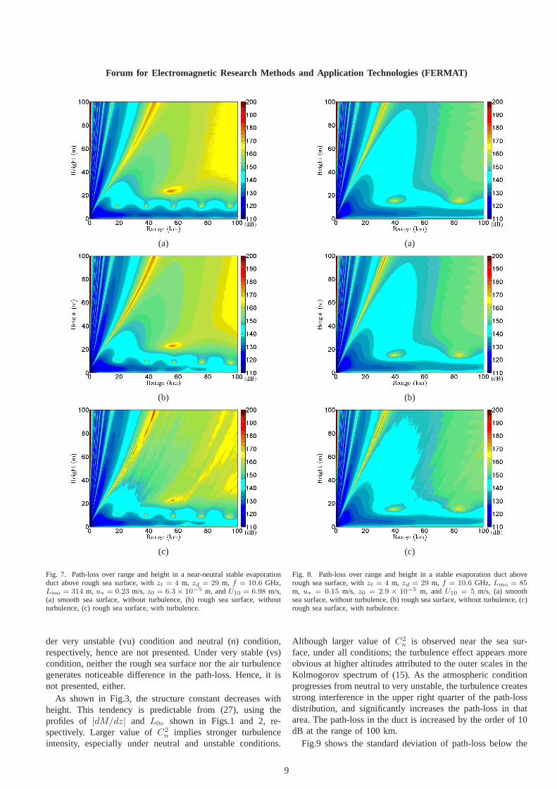
Fig. 7. Path-loss over range and height in a near-neutral stable evaporationduct above rough sea surface, withzt = 4 m, zd = 29 m, f = 10.6 GHz,Lmo = 314 m, u∗ = 0.23 m/s, z0 = 6.3× 10−5 m, andU10 = 6.98 m/s,(a) smooth sea surface, without turbulence, (b) rough sea surface, withoutturbulence, (c) rough sea surface, with turbulence.

der very unstable (vu) condition and neutral (n) condition,respectively, hence are not presented. Under very stable (vs)condition, neither the rough sea surface nor the air turbulencegenerates noticeable difference in the path-loss. Hence, it isnot presented, either.

As shown in Fig.3, the structure constant decreases withheight. This tendency is predictable from (27), using theprofiles of |dM/dz| and L0v shown in Figs.1 and 2, re-spectively. Larger value ofC2

n implies stronger turbulenceintensity, especially under neutral and unstable conditions.

(a)

(b)

(c)

Fig. 8. Path-loss over range and height in a stable evaporation duct aboverough sea surface, withzt = 4 m, zd = 29 m, f = 10.6 GHz, Lmo = 85m, u∗ = 0.15 m/s, z0 = 2.9 × 10−5 m, andU10 = 5 m/s, (a) smoothsea surface, without turbulence, (b) rough sea surface, without turbulence, (c)rough sea surface, with turbulence.

Although larger value ofC2n is observed near the sea sur-

face, under all conditions; the turbulence effect appears moreobvious at higher altitudes attributed to the outer scales in theKolmogorov spectrum of (15). As the atmospheric conditionprogresses from neutral to very unstable, the turbulence createsstrong interference in the upper right quarter of the path-lossdistribution, and significantly increases the path-loss inthatarea. The path-loss in the duct is increased by the order of 10dB at the range of 100 km.

Fig.9 shows the standard deviation of path-loss below the

9


(a)

(b)

(c)

(d)

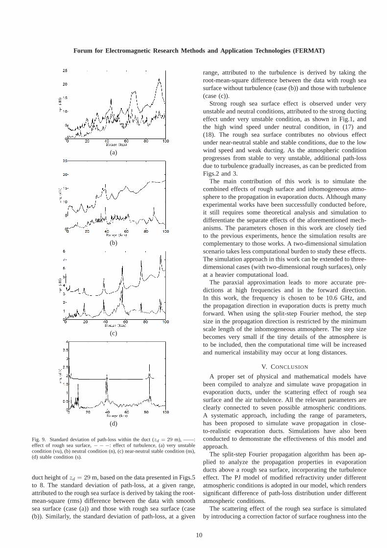
Fig. 9. Standard deviation of path-loss within the duct (zd = 29 m), ——:effect of rough sea surface,− − −: effect of turbulence, (a) very unstablecondition (vu), (b) neutral condition (n), (c) near-neutral stable condition (ns),(d) stable condition (s).

duct height ofzd = 29 m, based on the data presented in Figs.5to 8. The standard deviation of path-loss, at a given range,attributed to the rough sea surface is derived by taking the root-mean-square (rms) difference between the data with smoothsea surface (case (a)) and those with rough sea surface (case(b)). Similarly, the standard deviation of path-loss, at a given

range, attributed to the turbulence is derived by taking theroot-mean-square difference between the data with rough seasurface without turbulence (case (b)) and those with turbulence(case (c)).

Strong rough sea surface effect is observed under veryunstable and neutral conditions, attributed to the strong ductingeffect under very unstable condition, as shown in Fig.1, andthe high wind speed under neutral condition, in (17) and(18). The rough sea surface contributes no obvious effectunder near-neutral stable and stable conditions, due to thelowwind speed and weak ducting. As the atmospheric conditionprogresses from stable to very unstable, additional path-lossdue to turbulence gradually increases, as can be predicted fromFigs.2 and 3.

The main contribution of this work is to simulate thecombined effects of rough surface and inhomogeneous atmo-sphere to the propagation in evaporation ducts. Although manyexperimental works have been successfully conducted before,it still requires some theoretical analysis and simulationtodifferentiate the separate effects of the aforementioned mech-anisms. The parameters chosen in this work are closely tiedto the previous experiments, hence the simulation results arecomplementary to those works. A two-dimensional simulationscenario takes less computational burden to study these effects.The simulation approach in this work can be extended to three-dimensional cases (with two-dimensional rough surfaces),onlyat a heavier computational load.

The paraxial approximation leads to more accurate pre-dictions at high frequencies and in the forward direction.In this work, the frequency is chosen to be 10.6 GHz, andthe propagation direction in evaporation ducts is pretty muchforward. When using the split-step Fourier method, the stepsize in the propagation direction is restricted by the minimumscale length of the inhomogeneous atmosphere. The step sizebecomes very small if the tiny details of the atmosphere isto be included, then the computational time will be increasedand numerical instability may occur at long distances.

V. CONCLUSION

A proper set of physical and mathematical models havebeen compiled to analyze and simulate wave propagation inevaporation ducts, under the scattering effect of rough seasurface and the air turbulence. All the relevant parametersareclearly connected to seven possible atmospheric conditions.A systematic approach, including the range of parameters,has been proposed to simulate wave propagation in close-to-realistic evaporation ducts. Simulations have also beenconducted to demonstrate the effectiveness of this model andapproach.

The split-step Fourier propagation algorithm has been ap-plied to analyze the propagation properties in evaporationducts above a rough sea surface, incorporating the turbulenceeffect. The PJ model of modified refractivity under differentatmospheric conditions is adopted in our model, which renderssignificant difference of path-loss distribution under differentatmospheric conditions.

The scattering effect of the rough sea surface is simulatedby introducing a correction factor of surface roughness into the

10


boundary condition. When the atmosphere is more unstable,the interference pattern within a duct bears a shorter periodand a wider range of path-loss variation.

The turbulence is described with a two-dimensional Kol-mogorov spectrum, in which the structure constant of refrac-tive index fluctuation, the outer scales of turbulence, and theanisotropy of the outer scales are well connected to differentatmospheric conditions.

Significant effects of rough sea surface and air turbulenceare observed under neutral (|Lmo| ∼ ∞) and unstable (Lmo <0) conditions. The effect of rough sea surface is less significantunder stable (Lmo > 0) conditions, accompanied by lowgrazing angle and low wind speed. The effect of air turbulencegradually increases as the atmospheric condition progressesfrom stable to unstable, accompanied by larger eddy size andstronger turbulence intensity.

REFERENCES

[1] A. V. Kukushkin, V. D. Freilikher, and I. M. Fuks, “Transhorizon prop-agation of ultrashort radio waves above the sea (review),”Radiofizika,vol.30, no.7, pp.811-839, 1987.

[2] K. V. Koshel and A. A. Shishkarev, “Influence of layer and anisotropicfluctuations of the refractive index on the beyond-the-horizon SHFpropagation in the troposphere over the sea when there is an evaporationduct,” Waves in Random Media, vol.3, no.1, pp.25-38, 1993.

[3] F. T. Ulaby, R. K. Moore, and A. K. Fung, “Microwave remote sensingfundamentals and radiometry,” inMicrowave Remote Sensing: Activeand Passive, vol. 1, Addison-Wesley, 1981.

[4] F. Mesnard and H. Sauvageot, “Climatology of anomalous propagationradar echoes in a coastal area,”J. Appl. Meteorol. Climatol., vol.49,no.11, pp. 2285-2300, 2010.

[5] M. I. Skolnik, Introduction to Radar Systems, 3rd ed., McGraw-Hill,2001.

[6] R. Douvenot, V. Fabbro, P. Gerstoft, C. Bourlier, and J. Saillard, “A ductmapping method using least squares support vector machines,”RadioSci., vol.43, pp.1-12, 2008.

[7] K. D. Anderson, “Radar measurements at 16.5 GHz in the oceanic evap-oration duct,” IEEE Trans. Antennas Propagat., vol.37, no.1, pp.100-106, 1989.

[8] B. W. Atkinson, J-G. Li, and R. S. Plant, “Numerical modeling of thepropagation environment in the atmospheric boundary layer over thePersian Gulf,”J. Appl. Meteorol. Climatol., vol.40, no.3, pp.586-603,2001.

[9] A. Kerans, A. S. Kulessa, E. Lensson, G. French, and G. S. Woods,“Implications of the evaporation duct for microwave radio path designover tropical oceans in Northern Australia,”Workshop Appl. Radio Sci.,Leura, Australia, 2002.

[10] I. Sirkova and M. Mikhalev, “Parabolic-equation-based study of ductingeffects on microwave propagation,”Microwave Opt. Technol. Lett.,vol.42, no.5, pp.390-394, 2004.

[11] I. Sirkova and M. Mikhalev, “Influence of tropospheric ducting onmicrowave propagation in short distances,”EURO-COST 273 TD(02)086, Espoo, Finland, 2002.

[12] I. Sirkova and M. Mikhalev, “Influence of tropospheric duct parameterschanges on microwave path loss,”Proc. Int. Sci. Conf. Inf. Commun.Energy Syst. Technol., Sofia, Bulgaria, pp.43-46, 2003.

[13] S. S. Mentes and Z. Kaymaz, “Investigation of surface duct conditionsover Istanbul, Turkey,”J. Appl. Meteorol. Climatol., vol.46, no.3, pp.318-337, 2007.

[14] I. Sirkova, “Path loss calculation for a surface duct statistics,”Proc. Int.Sci. Conf. Inf. Commun. Energy Syst. Technol., Veliko Tarnovo, Bulgaria,pp.53-56, 2009.

[15] H. Hitney and R. Vieth, “Statistical assessment of evaporation ductpropagation,”IEEE Trans. Antennas Propagat., vol.38, no.6, pp.794-799, 1990.

[16] H. V. Hitney and L. R. Hitney, “Frequency diversity effects of evapora-tion duct propagation,”IEEE Trans. Antennas Propagat., vol.38, no.10,pp.1694-1700, 1990.

[17] R. A. Paulus, “Practical application of an evaporationduct model,”RadioSci., vol.20, no.4, pp.887-896, 1985.

[18] A. Kukushkin and J. Wiley,Radio Wave Propagation in the MarineBoundary Layer, Wiley Online Library, 2004.

[19] H. V. Hitney, “Evaporation duct propagation and near-grazing anglescattering from a rough sea,”IEEE Int. Geosci. Remote Sensing Symp.,pp.2631-2633, 1999.

[20] D. Rouseff, “Simulated microwave propagation through troposphericturbulence,” IEEE Trans. Antennas Propagat., vol.40, no.9, pp.1076-1083, 1992.

[21] H. V. Hitney, “A practical tropospheric scatter model using the parabolicequation,” IEEE Trans. Antennas Propagat., vol.41, no.7, pp.905-909,1993.

[22] A. Barrios, “Modeling surface layer turbulence effects at microwavefrequencies,”IEEE Radar Conf., 2008.

[23] I. Levadnyi, V. Ivanov, and V. Shalyapin, “Simulation ofmicrowavepropagation in turbulent evaporation duct,”Euro, Conf. Antennas Prop-agat., 2012.

[24] M. Levy, Parabolic Equation Methods for Electromagnetic Wave Prop-agation, Inst. Electr. Eng., 2000.

[25] O. Benhmammouch, N. Caouren, and A. Khenchaf, “Influence ofseasurface roughness on electromagnetic waves propagation in presence ofevaporation duct,”Int. Radar Conf., 2009.

[26] T. S. Hristov, K. D. Anderson, and C. A. Friehe, “Scattering propertiesof the ocean surface: the Miller-Brown-Vegh model revisited,” IEEETrans. Antennas Propagat., vol.56, no.4, pp.1103-1109, 2008.

[27] Y. V. Levadnyi, V. K. Ivanov, and V. N. Shalyapin, “Simulation ofmicrowave propagation in evaporation duct over rough sea surface (inRussian),”Radiophys. Electron., vol.14, pp.28-34, 2004.

[28] J. R. Kuttler and G. D. Dockery, “Theoretical description of the parabolicapproximation/Fourier split-step method of representing electromagneticpropagation in the troposphere,”Radio Sci., vol.26, no.2, pp.381-393,1991.

[29] G. Apaydin and L. Sevgi, “FEM-based surface wave multimixed-pathpropagator and path loss predictions,”IEEE Antennas Wireless Propagat.Lett., vol.8, pp.1010-1013, 2009.

[30] A. S. Kulessa, G. S. Woods, B. Piper, and M. L. Heron, “Line-of-sight EM propagation experiment at 10.25 GHz in the tropical oceanevaporation duct,”IEE Proc. Microwaves Antennas Propagat., vol.145,no.1, pp.65-69, 1998.

[31] H. Essen and H. H. Fuchs, “Microwave and millimeterwave propagationwithin the marine boundary layer,”German Microwave Conf., Karlsruhe,Germany, 2006.

[32] S. D. Gunashekar, E. M. Warrington, D. R. Siddle, and P. Valtr, “Signalstrength variations at 2 GHz for three sea paths in the British channelislands: Detailed discussion and propagation modeling,”Radio Sci.,vol.42, no.4, pp.1-13, 2007.

[33] V. K. Ivanov, V. N. Shalyapin, and Y. V. Levadny, “Microwave scat-tering by tropospheric fluctuations in an evaporation duct,” Radiophys.Quantum Electron., vol.52, no.4, pp.277-286, 2009.

[34] G. Bein, “Monte Carlo computer technique for one-dimensional randommedia,” IEEE Trans. Antennas Propagat., vol.21, no.1, pp.83-88, 1973.

[35] R. N. Adams and E. D. Denman,Wave Propagation and TurbulentMedia, Elsevier, 1966.

[36] G. L. Geernaert, “On the evaporation duct for inhomogeneous conditionsin coastal regions,”J. Appl. Meteorol. Climatol., vol.46, no.4, pp.538-543, 2007.

[37] S. A. Raid, J. Z. Gehman, J. R. Kuttler, and M. H. Newkirk, “Modelingradar propagation in three-dimensional environments,”Johns HopkinsAPL Tech. Digest, vol.25, no.2, p.101, 2004.

[38] R. Janaswamy, “Path loss predictions in the presence of buildings onflat terrain: A 3-D vector parabolic equation approach,”IEEE Trans.Antennas Propagat., vol.51, no.8, pp.1716-1728, 2003.

[39] J. P. Zhang, Z. S. Wu, Q. L. Zhu, and B. Wang, “A four-parameterm-profile model for the evaporation duct estimation from radar clutter,”Prog. Electromag. Res., vol.114, pp.353-368, 2011.

[40] G. D. Dockery, R. Awadallah, D. E. Freund, J. Z. Gehman, and M.H. Newkirk, “An overview of recent advances for the TEMPER radarpropagation model,”IEEE Radar Conf., pp.896-905, 2007.

[41] R. Frehlich, “Simulation of laser propagation in a turbulent atmosphere,”Appl. Opt., vol.39, no.3, pp.393-397, 2000.

[42] A. R. Miller, R. M. Brown, and E. Vegh, “New derivation for therough-surface reflection coefficient and for the distribution of sea-waveelevations,” IEE Proc. H: Microwaves Opt. Antennas, vol.131, no.2,pp.114-116, 1984.

[43] D. Dockery and J. R. Kuttler, “An improved impedance-boundary algo-rithm for Fourier split-step solutions of the parabolic wave equation,”IEEE Trans. Antennas Propagat., vol.44, no.12, pp.1592-1599, 1996.

11


[44] W. L. Patterson, C. P. Hattan, H. V. Hitney, R. A. Paulus,and G.E. Lindem, “Engineer’s refractive effects prediction system (EREPS)version 3.0,” DTIC Doc. ADA283748, 1994.

[45] D. E. Freund, N. E. Woods, H. C. Ku, and R. S. Awadallah, “The effectsof shadowing on modelling forward radar propagation over a rough seasurface,”Waves Random Complex Medium, vol.18, pp.387-408, 2008.

[46] G. I. Taylor, “The spectrum of turbulence,”Proc. R. Soc. London, Ser.A, vol.164, no.919, pp.476-490, 1938.

[47] A. Ishimaru,Wave Propagation and Scattering in Random Media, IEEEPress, 1997.

[48] N. Wiener, “Generalized harmonic analysis,”Acta Mathematica, vol.55,no.1, pp.117-258, 1930.

[49] R. A. Paulus, “Specification for environmental measurements to assessradar sensors,” DTIC Doc., 1989.

[50] H. A. Panovsky and J. A. Dutton,Atmospheric Turbulence: Models andMethods for Engineering Applications, John Wiley, 1984.

[51] S. E. Gryning, E. Batchvarova, B. Brummer, H. Jørgensen, and S.Larsen, “On the extension of the wind profile over homogeneousterrainbeyond the surface boundary layer,”Boundary Layer Meteorol., vol.124,no.2, pp.251-268, 2007.

[52] A. Pena, S. E. Gryning, and C. B. Hasager, “Measurements andmodelling of the wind speed profile in the marine atmospheric boundarylayer,” Boundary Layer Meteorol., vol.129, no.3, pp.479-495, 2008.

[53] V. I. Tatarskii, The Effects of the Turbulent Atmosphere on WavePropagation, Israel Program for Scientific Translations, 1971.

[54] Z. Sorbjan,Structure of the Atmospheric Boundary Layer, Prentice Hall,1989.

[55] A. Ludi and A. Magun, “Near-horizontal line-of-sight millimeter-wavepropagation measurements for the determination of outer length scalesand anisotropy of turbulent refractive index fluctuations in the lowertroposphere,”Radio Sci., vol.37, no.2, pp.12.1-19, 2002.

[56] A. Ludi and A. Magun, “Refractivity structure constant and lengthscales from mm-wave propagation in the stably stratified troposphere,”J. Atmos. Sol. Terr. Phys., vol.67, no.5, pp.435-447, 2005.

[57] R. Soucy, R. Woodward, and H. A. Panofsky, “Vertical cross-spectra ofhorizontal velocity components at the Boulder observatory,” BoundaryLayer Meteorol., vol.24, no.1, pp.57-66, 1982.

[58] A. J. Bowen, R. G. J. Flay, and H. A. Panofsky, “Vertical coherence andphase delay between wind components in strong winds below 20 m,”Boundary Layer Meteorol., vol.26, no.4, pp.313-324, 1983.

[59] D. C. Cox, H. W. Arnold, and H. H. Hoffman, “Observations of cloud-produced amplitude scintillation on 19-and 28-GHz Earth-space paths,”Radio Sci., vol.16, no.5, pp.885-907, 1981.

[60] A. Tunick, “Optical turbulence effects on ground to satellite microwaverefractivity,” DTIC Doc. ADA449682, 2006.

[61] S. D. Burk, “Refractive index structure parameters-time-dependent cal-culations using a numerical boundary-layer model,”J. Appl. Meteorol.,vol.19, pp.562-576, 1980.

[62] A. S. Kulessa, M. L. Heron, and G. S. Woods, “Temporal variations inevaporation duct heights,”Proc. WARS’97, pp.165-170, 1997.

[63] J. D. Turton, D. A. Bennetts, and S. F. G. Farmer, “An introduction toradio ducting,”Meteorol. Mag., vol.117, no.1393, pp.245-254, 1988.

[64] A. Kerans, A. S. Kulessa, E. Lensson, G. French, and G. S.Woods,“Implications of the evaporation duct for microwave radio path designover tropical oceans in Northern Australia,”Proc. WARS’02, Leura,Australia, 2002.

[65] A. Kerans, G. S. Woods, E. Lensson, and G. French, “Propagation at 10.6GHz over a long path in the tropical evaporation duct,”Proc. WARS’02,Leura, Australia, 2002.

Yung-Hsiang Chou was born in Taipei, Taiwan,on March 25, 1989. He received the B.S. degree inelectrical engineering from National Central Univer-sity, Jhongli, Taiwan, in 2011 and the M.S. degreein communication engineering from National TaiwanUniversity, Taipei, Taiwan, in 2013.

Jean-Fu Kiang received his Ph.D. degree in elec-trical engineering, from the Massachusetts Instituteof Technology in 1989. He has been a professor ofthe Department of Electrical Engineering and theGraduate Institute of Communication Engineering,National Taiwan University since 1999. antennas andarrays, radar and navigation, RF and microwave sys-tems He has been interested in electromagnetic ap-plications and system issues, including wave propa-gation in different environments,antennas and arrays,radar and navigation, RF and microwave systems.

12

Forum for Electromagnetic Research Methods and Application Technologies (FERMAT)

Editorial Comment

In this article the authors present a computationally efficient algorithm for multi-feature

image reconstruction. They choose the M87 galaxy in the center of Virgo cluster for their

simulation. The authors claim that the algorithm is less sensitive to nose than the conventional

methods.

Effect of Turbulence on Wave Propagation in Evaporation Ducts above … · 2017-01-06 · Forum for...

Documents

Transcript of Effect of Turbulence on Wave Propagation in Evaporation Ducts above … · 2017-01-06 · Forum for...