The Effect of Product Misperception on Economic Outcomes:

Evidence from the Extended Warranty Market ∗

Jose Miguel Abito Yuval Salant

June 15, 2018

Abstract

Panel and experimental data are used to analyze the economic outcomes in the extended

warranty market. We establish that the strong demand and high profits in this market are driven

by consumers distorting the failure probability of the insured product, rather than standard risk

aversion or sellers’ market power. Providing information to consumers about failure probabilities

significantly reduces their willingness to pay for warranties, indicating the important role of

information, or lack of, in driving consumers’ purchase behavior. Such information provision is

shown to be more effective in enhancing consumer welfare than additional market competition.

∗ Abito: University of Pennsylvania, Wharton School, Business Economics and Public Policy, abito@wharton.upenn.edu. Salant: Northwestern University, Kellogg School of Management, Department of Managerial Economics and Decision Sciences, y-salant@kellogg.northwestern.edu. We thank Heski Bar-Isaac, JF Houde, Ulrich Doraszelski, Katja Seim, Eduardo Azevedo, Joe Harrington, Jeremy Tobacman, Tom Baker, Chris Conlon, Christian Michel, Sanket Patil, Nicola Persico, and the editor and four anonymous referees for helpful comments. Salant also thanks Nabil Al-Najjar and an anonymous student for early discussions on the extended warranty market.

1

1 Introduction

An extended warranty is an insurance contract that protects against the failure of a durable good

such as a consumer electronic. The extended warranty market is highly profitable,1 and has caught

the attention of consumer protection and competition authorities in different countries. In the

UK, the Office of Fair Trading observed that “there is insufficient competition and information to

ensure that consumers get good value” in the extended warranty market, and that “many electrical

retailers may make considerable profits on the sale of extended warranties” (UK Competition Com-

mission, 2003). The UK Competition Commission has consequently conducted a comprehensive

investigation of this market. Its report expressed concerns about the lack of market competition due

to the way warranties are sold, and the lack of available information at the point of sale about the

reliability of the insured product and the cost of repair (UK Competition Commission, 2003). The

Federal Trade Commission in the US has also looked into this market, and is advising consumers

to obtain information about the likelihood of product failure and the potential cost of repair before

buying an extended warranty.2

This paper uses panel and experimental data to analyze market competition and consumer

behavior in the extended warranty market. The first takeaway from the analysis is that the strong

demand and high profits in this market are driven by consumers distorting the failure probability

of the insured product, rather than standard risk aversion or sellers’ market power. The second

takeaway is that providing information to consumers about failure probabilities significantly reduces

their willingness to pay for warranties, indicating the important role of information, or lack of, in

driving consumers’ purchase behavior. The third takeaway is that such information provision is

more effective in enhancing consumer welfare than additional market competition, highlighting the

relevance of policies that guide consumers’ decision making directly.

The starting point of our analysis is that the market for extended warranties is characterized by

market power on the supply side and high willingness to pay on the demand side. On the supply

side, sellers have market power because the warranty is an add-on product. It is usually offered

to consumers immediately after they finalize their decision to buy the insured product,3 at a stage

in which searching for another product or switching to another seller is costly. This search and

switching cost implies significant market power a la Ellison’s (2005) add-on pricing model.4

1The UK Competition Commission (2003) estimates that the top five consumer electronics retailers in the UK earned 116 to 152 million pounds annually on the sale of extended warranties in the early 2000s. Similarly, analysts in the US estimate extended warranties accounted for almost half of BestBuy’s operating income in 2003, and that profit margins on warranties ranged from 50% to 60% (“The Warranty Windfall,” Business Week (December 19, 2004)).

2See https://www.consumer.ftc.gov/articles/0240-extended-warranties-and-service-contracts (accessed on June 15, 2018).

3For example, BestBuy trains its sales people to offer warranties to consumers only af-ter they finalize the TV purchase decision. For BestBuy’s presentation of selling skills, see https://www.extendingthereach.com/wps/PA VCorationFramework/resource?argumentRef=static&resourceRef=/files/Best Buy Vendor Selling Skills.pdf

(accessed on June 15, 2018). 4According to the UK Competition Commission (2003), “Most customers shop around for electronic goods; the

retail price is a major factor in their choice. However, extended warranty buyers do not often plan to buy an extended

2

On the demand side, about one in four TV buyers in our panel data purchases an extended

warranty. On average, this buyer pays $90 or more to insure against a loss of at most $400 with

7% probability. What drives this high willingness to pay? Sydnor (2010) uses data on home

insurance deductible choices to show standard risk aversion in the form of diminishing marginal

utility for wealth cannot explain consumers’ high willingness to pay for reductions in deductibles.

Sydnor (2010) proposes several alternative explanations for the high willingness to pay, including

misperception of claim probabilities and reference-dependent preferences. Barseghyan et al. (2013)

examine several alternatives to standard risk aversion, and conclude that upward distortion of claim

probabilities plays a key role in explaining deductible choices in home and auto insurance.

Our first objective is to quantify the importance of probability distortions and standard risk

aversion on the demand side relative to market power on the supply side in determining demand,

prices, and profits in the extended warranty market.

To do so, we consider a model of market competition based on Ellison’s (2005) add-on pricing

game to which we incorporate Barseghyan et al.’s (2013) decision-making model, in which consumers

are assumed to be risk-averse expected utility maximizers who may distort failure probabilities. We

then use panel data on household-level product and extended warranty purchases from a large US

electronics retailer to estimate consumers’ risk-aversion and probability-distortion parameters and

the retailer’s cost of selling and servicing the warranty. The panel data documents approximately

45,000 transactions made by almost 20,000 households between 1998 and 2004. Almost 30% of

the transactions involved the purchase of an extended warranty. Our structural estimation focuses

on TVs, which constitute about 11% of the data, due to the availability of TV failure rates from

Consumer Reports.

Variation in repair costs for different products with the same failure rate enables us to sepa-

rately identify the risk-aversion and probability-distortion parameters. Intuitively, either parameter

can explain the willingness to pay for a warranty to any given product. But they have different

predictions regarding the rate at which willingness to pay changes in response to a change in the

repair cost. In particular, probability distortion implies a slower rate than risk aversion. Thus,

fixing the failure rate, changes in willingness to pay in response to changes in repair costs enable

us to separately identify the two parameters.

Our estimation indicates there is a substantial upward distortion of failure probabilities. For

example, a 5% objective failure probability is perceived as a 13% failure probability. This estimate

is similar to the estimate of Barseghyan et al. (2013) and to results from our experiment described

below. Standard risk aversion, on the other hand, plays an insignificant role in consumers’ decision

making. The estimated risk-aversion parameter implies willingness to pay is close to actuarially

fair rates in the absence of probability distortion.

We use counterfactual analysis to quantify the effect of probability distortions on market out-

warranty (less than half of consumers who bought an extended warranty said that they had planned to do so before they went into the store), and many are unaware of the existence of alternatives to taking the EW offered at the point of sale.”

3

comes. Specifically, we compare outcomes in the existing market with outcomes in a counterfactual

market in which retailers have the same market power but the distortion is “shut down” in the

sense that consumers use objective failure probabilities in decision making. A key assumption in

the analysis is that TVs are priced similarly whether consumers distort failure probabilities or not.

As discussed in section 7, this assumption is supported by comparing TV prices between retailers

who offer extended warranties and retailers who do not, institutional details, and Ellison’s (2005)

results.

The counterfactual analysis demonstrates that probability distortions drive the strong demand

and high profits, whereas market power drives the high prices and margins. Specifically, when

shutting down probability distortions, volume and profit decrease by more than 90%, but price and

margin decrease by only 4% and 11%, respectively.

Our second objective is to better understand the mechanism for the distortion. One possible

mechanism is that consumers know the objective probabilities but overweigh them as predicted by

Prospect Theory (Kahneman and Tversky (1979)). Another possible mechanism — which seems to

fit the concerns of competition authorities — is that consumers lack information about the objective

probabilities and overestimate them. Bordalo et al.’s (2015) theory of attention proposes a possible

reason for overestimation: consumers are surprised when reminded by the sales person that TVs

can break, and overreact to this information.5

Understanding the mechanism is welfare- and policy-relevant. If the distortion stems from lack

of information about failure probabilities, as postulated by the second mechanism, consumer welfare

should be evaluated with respect to the objective probabilities, and room exists for policies that

inform consumers about these probabilities. On the other hand, if consumers know the probabilities

and distort them in their decision making, deciding whether objective or distorted probabilities

should be used in welfare analysis depends on whether one interprets overweighting as a deliberate

process or as a mistake in decision making.6

To study the mechanism, we conducted experiments. In a pretest with approximately 500

participants, we found the failure rate in the pool of participants was about 5%. This rate is

similar to the failure rates reported by Consumer Reports.

In the first main experiment with approximately 1,000 participants who did not participate in

the pretest, we randomly assigned participants to one of three treatments. In two treatments, we

elicited participants’ perceived TV failure probability and their willingness to pay for an extended

warranty, and in the third, we first informed participants about the objective probability and then

elicited their willingness to pay. We found that average perceived TV failure probability among

5Possible support for Bordalo et al.’s (2015) theory comes from the comparison of the strong in-store demand with the weak online demand in the data (see section 2.3.) Indeed, making TV failures salient and triggering overreaction seems harder in the online marketplace than in the store, where the sales person has the buyer’s attention, and can press the buyer to make a quick decision.

6This mechanism-based approach to welfare analysis is based on Rubinstein and Salant (2008, 2012) who argue behavioral welfare analysis should rely on understanding the mechanism that maps the decision maker’s preferences to his choices.

4

uninformed participants was about 14%, which is almost three times larger than the objective fail-

ure rate. Moreover, the average willingness to pay among informed participants was much lower

than among uninformed participants. For example, the median willingness to pay among informed

participants was about half of the median willingness to pay among uninformed participants. We

interpret these findings as suggesting that lack of information about failure probabilities is a rel-

evant factor in creating the distortion, and that information provision reduces willingness to pay

significantly.

In the second experiment with another 900 participants, we examined whether traces of prob-

ability distortion were present among informed participants. Specifically, we elicited informed

participants’ willingness to pay for TVs with the same failure rate but with different repair costs,

and used the identification strategy of the empirical analysis to separately identify the risk aversion

and probability distortion parameters from the reported willingness to pay. We found that most

participants displayed modest or no probability distortion as well as no risk aversion. We interpret

these findings as indicating information provision reduces the distortion significantly.

Equipped with the experimental findings, our third objective is to evaluate consumer welfare

and the effectiveness of various policy interventions based on the panel data. We first observe that

welfare in the existing market is negative, i.e., consumer welfare would increase if the market for

warranties did not exist. This is because any positive welfare generated by warranty purchases

of buyers with true willingness to pay above price is dominated by the decrease in welfare due

to warranty purchases of buyers with true willingness to pay below price who overestimate failure

probabilities.

As for policy, Armstrong (2008) discusses two broad categories of policies competition author-

ities use to enhance market performance and consumer welfare. The first and more prominent

category includes competition policies, which target the supply side of the market and aim to in-

tensify competition. The second category includes consumer policies, which target the demand side

and aim to enhance consumers’ decision making directly.

An example of a competition policy in the extended warranty market is the UK Competition

Commission’s (2003) proposal that retailers advertise and post the price of the warranty alongside

the price of the product it insures. This policy is expected to drive down prices because it reduces

the search and switching costs of consumers. If the demand for warranties were driven solely by

consumers’ risk aversion, such a price reduction would have a positive effect on consumer welfare.

It would increase the utility of existing warranty buyers as well as the utility of new buyers, who

now purchase the warranty because of the lower prices. But with overestimation, the utility of new

buyers may be negative, and so the effect of price reduction on consumer welfare is unclear. On the

other hand, a consumer policy that reduces overestimation increases consumer welfare, assuming

no price change, because consumers make better choices, but may trigger a price change, and so

its effect is also unclear. An example of a consumer policy is to demand retailers to disclose failure

probabilities to consumers, similar to what we did in the experiment.

5

Counterfactual analysis demonstrates that consumer policies that reduce overestimation are

more effective in enhancing consumer welfare than competition policies that lead to price reduction.

Intuitively, when warranty prices go down but overestimation still exists, consumer welfare decreases

because the welfare gain due to lower prices is dominated by the welfare loss generated by more

consumers buying warranties due to overestimation. On the other hand, when overestimation goes

down, consumer welfare increases because the welfare gain due to consumers making better choices

dominates any other effect. Thus, our findings indicate competition policies may lead to suboptimal

results in markets with uninformed or biased consumers relative to consumer policies that aim to

improve consumers’ decision making directly.

The rest of the paper is organized as follows. Section 1.1 reviews the related literature. Section 2

presents the panel data and reports empirical regularities on household purchase behavior. Section 3

presents the model and the identification strategy. Section 4 describes the estimation procedure.

Section 5 reports the results of the estimation. Section 6 studies the mechanism for the distortion.

Section 7 studies the importance of probability distortions relative to market power in determining

demand, prices, profit, and consumer welfare. Section 8 concludes with a discussion of policy

implications.

1.1 Related literature

This paper is related to the empirical literature on estimating risk preferences (see Barseghyan

et al. (forthcoming) for a recent survey.) Cohen and Einav (2007) use data on auto insurance

deductible choices to estimate a structural model of individual choice with standard risk aversion.

They find unobserved heterogeneity in risk aversion is greater than unobserved heterogeneity in

risk (claim rates), and that the two are positively correlated. Barseghyan et al. (2011) compare

households’ degree of standard risk aversion in auto and home insurance. They find risk preferences

are not stable across contexts, and that many households exhibit greater risk aversion in their home

deductible choices than in their auto deductible choices.

Sydnor (2010) uses home insurance deductible choices to demonstrate that consumers’ will-

ingness to pay for insurance is very high. For example, many consumers pay $100 to lower their

deductible from $1,000 to $500 when their (ex-post) claim rate is less than 5%. Sydnor (2010)

shows that fitting such choices to a model with standard risk aversion yields extreme levels of risk

aversion, and proposes several alternative explanations for the high willingness to pay, including

misperception of claim rates and reference-dependent preferences.

Our paper is closest to Barseghyan et al. (2013), who develop a structural model of individ-

ual choice with standard risk aversion and probability distortions, and estimate it using data on

auto and home insurance deductible choices. Barseghyan et al. (2013) find upward distortion

of claim probabilities plays a key role in explaining deductible choices. Moreover, the shape of

the probability-distortion function fits the shape predicted by Prospect Theory (Kahneman and

Tversky (1979)). Several other papers incorporate probability distortions to the estimation of risk

6

2

preferences, and find evidence of their relevance in various contexts, including financial markets

(Kliger and Levy (2009)) and betting markets (Jullien and Salanie (2000), Snowberg and Wolfers

(2010), Chiappori et al. (2012), Gandhi and Serrano-Padial (2014)).

We make three contributions to this literature. First, we quantify the effect of probability

distortions, relative to market power and risk aversion, on prices, volume, and profit. We are able

to make progress on this question because electronics retailers have (1) monopolistic power when

selling warranties, which facilitates cost estimation, and (2) little flexibility in cutting TV prices

below cost, which facilitates the counterfactual analysis. Second, we use experimental data to

show the distortion stems from lack of information about failure probabilities. This contribution is

important for welfare analysis and the evaluation of policy interventions. Third, we demonstrate

that consumer policies are more effective than competition policies in improving consumer welfare.

Another related literature is the marketing and experimental literature on why consumers buy

extended warranties (Chen et al. (2009), Huysentruyt and Read (2010), Jindal (2014)). Chen et

al. (2009) use purchase data of about 600 households from an unspecified US electronics retailer

over the period November 2003 to October 2004 to study how the insured product characteristics

(hedonic vs. utilitarian) and marketing actions by retailers affect the likelihood of purchasing an

extended warranty. Huysentruyt and Read (2010) use survey data to demonstrate that participants

overestimate the likelihood of washing-machine breakdowns and their cost of repair. Jindal (2014)

uses different survey data to highlight the role of loss aversion in the context of extended warranties

for washing machines. The four-year failure probability of washing machines is 20% to 30%, so

probability distortions are expected to have a less significant role in this context. We contribute

to this literature by demonstrating that lack of information about failure probabilities is a relevant

factor in creating the distortion, and that information provision significantly reduces the distortion.

Data

This section describes the panel data.

We use the INFORMS Society of Marketing Science Durables Dataset 1, which is a panel data of

household durable-goods transactions from a major US electronics retailer. The full sample contains

approximately 140,000 product-level transactions made by almost 20,000 households across the

retailer’s 1,176 outlets and its online store. Prices across outlets and the online store are essentially

identical. Transactions took place between December 1998 and November 2004.

The data contains four main types of transactions. About 117,000 transactions involve the

purchase of a specific product other than an extended warranty. About 15,000 transactions involve

the purchase of an extended warranty. About 5,000 transactions involve the return of a product

other than an extended warranty, and about 1,000 transactions involve the return of an extended

warranty. For each transaction, we observe the product ID, the price of the product, the brand,

and the category and subcategory of the product.

7

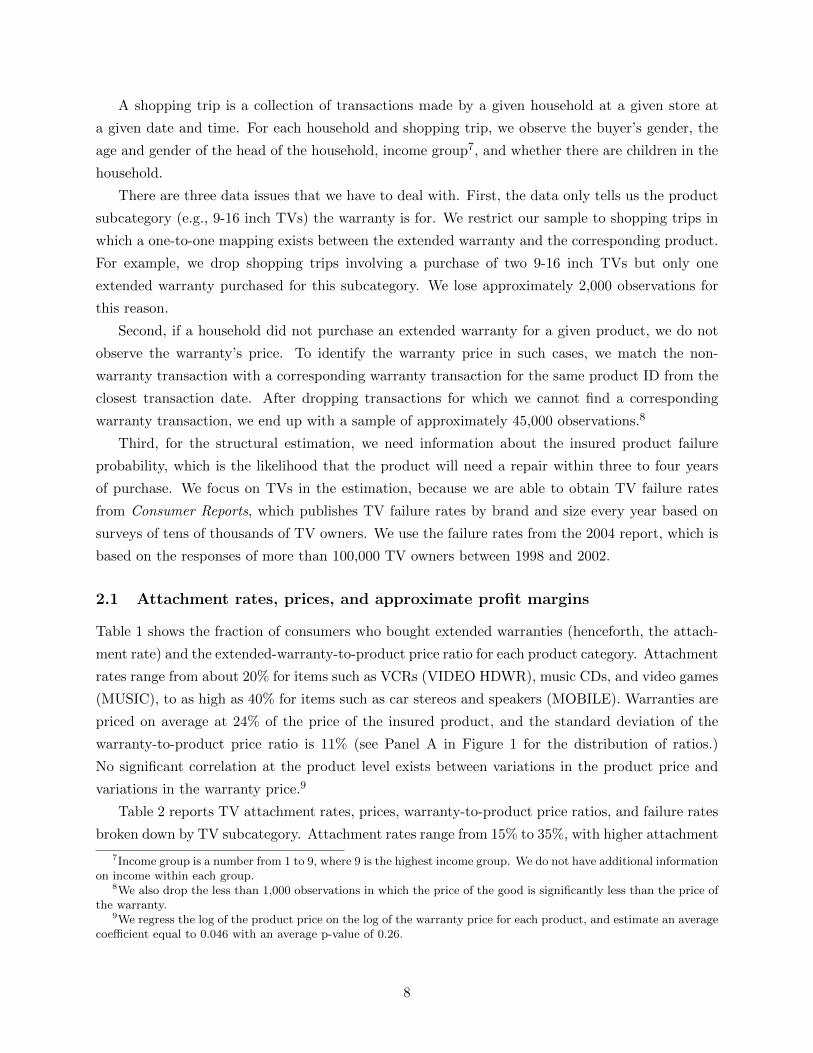
A shopping trip is a collection of transactions made by a given household at a given store at

a given date and time. For each household and shopping trip, we observe the buyer’s gender, the

age and gender of the head of the household, income group7, and whether there are children in the

household.

There are three data issues that we have to deal with. First, the data only tells us the product

subcategory (e.g., 9-16 inch TVs) the warranty is for. We restrict our sample to shopping trips in

which a one-to-one mapping exists between the extended warranty and the corresponding product.

For example, we drop shopping trips involving a purchase of two 9-16 inch TVs but only one

extended warranty purchased for this subcategory. We lose approximately 2,000 observations for

this reason.

Second, if a household did not purchase an extended warranty for a given product, we do not

observe the warranty’s price. To identify the warranty price in such cases, we match the non-

warranty transaction with a corresponding warranty transaction for the same product ID from the

closest transaction date. After dropping transactions for which we cannot find a corresponding

warranty transaction, we end up with a sample of approximately 45,000 observations.8

Third, for the structural estimation, we need information about the insured product failure

probability, which is the likelihood that the product will need a repair within three to four years

of purchase. We focus on TVs in the estimation, because we are able to obtain TV failure rates

from Consumer Reports, which publishes TV failure rates by brand and size every year based on

surveys of tens of thousands of TV owners. We use the failure rates from the 2004 report, which is

based on the responses of more than 100,000 TV owners between 1998 and 2002.

2.1 Attachment rates, prices, and approximate profit margins

Table 1 shows the fraction of consumers who bought extended warranties (henceforth, the attach-

ment rate) and the extended-warranty-to-product price ratio for each product category. Attachment

rates range from about 20% for items such as VCRs (VIDEO HDWR), music CDs, and video games

(MUSIC), to as high as 40% for items such as car stereos and speakers (MOBILE). Warranties are

priced on average at 24% of the price of the insured product, and the standard deviation of the

warranty-to-product price ratio is 11% (see Panel A in Figure 1 for the distribution of ratios.)

No significant correlation at the product level exists between variations in the product price and

variations in the warranty price.9

Table 2 reports TV attachment rates, prices, warranty-to-product price ratios, and failure rates

broken down by TV subcategory. Attachment rates range from 15% to 35%, with higher attachment

7Income group is a number from 1 to 9, where 9 is the highest income group. We do not have additional information on income within each group.

8We also drop the less than 1,000 observations in which the price of the good is significantly less than the price of the warranty.

9We regress the log of the product price on the log of the warranty price for each product, and estimate an average coefficient equal to 0.046 with an average p-value of 0.26.

8

Table 1: Attachment rate and price ratio by product category Attachment rate EW-Product price ratio Obs

AUDIO 0.281 0.232 6450 DVS 0.295 0.207 1439 IMAGING 0.377 0.199 3001 MAJORS 0.356 0.197 864 MOBILE 0.398 0.249 5176 MUSIC 0.208 0.169 1189 P*S*T 0.245 0.237 3765 PC HDWR 0.258 0.274 8773 TELEVISION 0.311 0.217 6307 VIDEO HDWR 0.206 0.240 5828 WIRELESS 0.245 0.317 1485 OVERALL 0.287 0.239 44277 Notes: Overall attachment weighted averages.

rates and EW-Product price ratios are sales-

Table 2: EW information for TVs Attach rate TV price EW-TV price ratio Fail rate Margin Obs

9-16in 0.149 122.99 0.284 0.072 0.729 422 19-20in 0.176 173.97 0.240 0.065 0.710 1067 25in 0.270 245.33 0.220 0.069 0.643 522 27in 0.299 354.06 0.197 0.059 0.681 1477 >30in 0.348 812.53 0.219 0.076 0.619 1229 OVERALL (TV) 0.268 400.07 0.223 0.067 0.672 4717 Notes: Fail rates are from Consumer Reports. Overall numbers are sales-weighted averages. Margin is computed as

(EW price - fail rate × TV price)/EW price.

rates for more expensive categories. The average price ratio for TVs is about 22% with a standard

deviation of 8% (see Panel B in Figure 1.)

Using the TV price multiplied by the TV failure rate as a rough estimate of the expected cost

of servicing a TV warranty, Table 2 also reports a “back of the envelope” profit margin on TV

warranties. This margin ranges from 62% to 73% for different TV subcategories, which is close to

what is cited in the popular press. We expect the seller in our dataset to have lower margins due

to revenue sharing with warranty providers and commissions to sales people.

2.2 Buyers’ characteristics

Tables 3 and 4 examine the relationship between attachment rates and buyers’ characteristics for

all product categories and for TVs. In Table 3, attachment rates are broken down by buyer gender,

gender and age of the head of the household, income, and whether there is a child in the household.

Income is the only characteristic that is strongly correlated with attachment rates for TVs and

all other product categories. For example, when moving from the highest to the lowest income

category, TV attachment rates increase by almost 11 percentage points in TV attachment rates.

Having a child seems to decrease TV attachment rates by 7 percentage points, but this effect goes

9

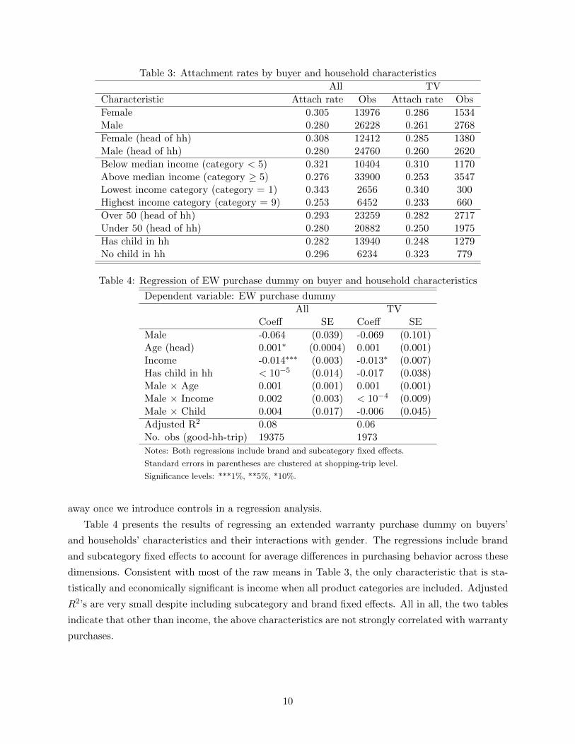
Table 3: Attachment rates by buyer and household characteristics All TV

Characteristic Attach rate Obs Attach rate Obs Female 0.305 13976 0.286 1534 Male 0.280 26228 0.261 2768 Female (head of hh) 0.308 12412 0.285 1380 Male (head of hh) 0.280 24760 0.260 2620 Below median income (category < 5) 0.321 10404 0.310 1170 Above median income (category ≥ 5) 0.276 33900 0.253 3547 Lowest income category (category = 1) 0.343 2656 0.340 300 Highest income category (category = 9) 0.253 6452 0.233 660 Over 50 (head of hh) 0.293 23259 0.282 2717 Under 50 (head of hh) 0.280 20882 0.250 1975 Has child in hh 0.282 13940 0.248 1279 No child in hh 0.296 6234 0.323 779

Table 4: Regression of EW purchase dummy on buyer and household characteristics

Dependent variable: EW purchase dummy All TV

Coeff SE Coeff SE Male -0.064 (0.039) -0.069 (0.101) Age (head) 0.001∗ (0.0004) 0.001 (0.001) Income -0.014∗∗∗ (0.003) -0.013∗ (0.007) Has child in hh < 10−5 (0.014) -0.017 (0.038) Male × Age 0.001 (0.001) 0.001 (0.001) Male × Income 0.002 (0.003) < 10−4 (0.009) Male × Child 0.004 (0.017) -0.006 (0.045) Adjusted R2 0.08 0.06 No. obs (good-hh-trip) 19375 1973 Notes: Both regressions include brand and subcategory fixed effects.

Standard errors in parentheses are clustered at shopping-trip level.

Significance levels: ***1%, **5%, *10%.

away once we introduce controls in a regression analysis.

Table 4 presents the results of regressing an extended warranty purchase dummy on buyers’

and households’ characteristics and their interactions with gender. The regressions include brand

and subcategory fixed effects to account for average differences in purchasing behavior across these

dimensions. Consistent with most of the raw means in Table 3, the only characteristic that is sta-

tistically and economically significant is income when all product categories are included. Adjusted

R2’s are very small despite including subcategory and brand fixed effects. All in all, the two tables

indicate that other than income, the above characteristics are not strongly correlated with warranty

purchases.

10

Table 5: Regression of extended warranty purchase dummy on shopping mode

Dependent variable: EW purchase dummy I II III IV V

In-store? 0.247*** 0.200*** 0.180*** 0.175*** 0.166*** (0.022) (0.027) (0.027) (0.027) (0.027)

Household FE N Y Y Y Y Subcategory FE N N Y Y Y Brand FE N N N Y Y Month FE N N N N Y Year FE N N N N Y No. obs 44304 44304 44304 44304 44304 (good-hh-trip) No. HHs 17158 17158 17158 17158 17158 Notes: Standard errors in parentheses are clustered at shopping-trip level.

2.3 In-store versus online transactions

About 1% of the transactions in the data were made online. The attachment rate for these trans-

actions is about 4%, which is one seventh of the in-store attachment rate. In Table 5, we use

regression analysis to examine what drives this difference and its robustness. The first model does

not include any controls, so it gives numbers that are similar to the raw attachment rates. The

other models turn on various fixed effects. Subcategory and brand fixed effects allow us to soak up

any differences in mean purchasing behavior induced by the nature of the product. We also include

household, month, and year fixed effects as further controls.

We see a drop in the effect of in-store purchases as we add fixed effects. Including a household

fixed effect reduces the effect by about 5 percentage points. Including product-related fixed effects

reduces the effect by additional 2.5 percentage points. Including all the fixed effects leads to a

reduction in the effect from 25 to 17 percentage points. That is, the likelihood of purchasing an

extended warranty jumps from 12% to 29% when the product is purchased in the store.

2.4 Warranty returns

The data contains 1,239 warranty return transactions. About 67% of them are returns that accom-

pany the insured product return. These returns are probably made due to the add-on feature of

the warranty – it has no value if the insured product is returned. But 33% of the warranty returns

are made without returning the main product. We run regressions similar to Table 4 and find that

none of the buyer or household characteristics in the data are strongly correlated with this return

behavior.

11

3 Theory

We consider an add-on pricing model a la Ellison (2005) and Ellison and Ellison (2009) to which

we incorporate the consumer model of Barseghyan et al. (2013).

There are several sellers of a main product M and an extended warranty EW for the product

M . Each seller sets a price p for the product that is observable to buyers, and a price t for the

warranty that is not.

The assumption that the product price is observable and the warranty price is not seems to be

the case in practice. For example, BestBuy advertises product prices but not warranty prices, and

trains its sales people to offer warranties and other add-ons to buyers only after they finalize their

decision to purchase the product.

Buyers decide which seller to visit after observing the price of the product across sellers and

forming rational expectations about warranty prices.10 Buyers visit the seller of their choice at a

cost s and learn the price of the warranty. The cost s corresponds to the hassle or time involved

in visiting a store and going through the purchase process. Buyers then decide whether to buy the

main product, the main product and the warranty, or visit another store at a cost of s, where they

will face the same decision.

Relevant equilibrium properties. As Ellison (2005) shows, any pure strategy sequential

equilibrium of the above game has two properties. The first is that the price of the warranty set by

any seller is the monopoly price relative to the demand for warranties among buyers of the product.

Otherwise, as in Diamond (1971), the seller can raise the price of the warranty by some � < s, and

buyers will not switch to another seller. We use the first-order condition of the monopoly pricing

problem to estimate the seller’s cost.

The second property is that buyers visit only one seller and always buy the product in equilib-

rium, because buyers incur a cost of visiting a seller. Thus, if they anticipate they will not buy the

main product, they will not visit the store. We therefore focus below on buyers’ decision to buy

the warranty conditional on already purchasing the product.

Warranty purchase decision. Following Barseghyan et al. (2013), we model buyers as

risk-averse expected utility maximizers who may distort failure probabilities.

Let W denote the buyer’s wealth after buying the main product, t the price of the warranty,

and u(·, r) the buyer’s concave utility over wealth levels that is parameterized by r, the buyer’s

degree of risk aversion around W .

A buyer’s utility if he purchases the warranty is VEW = u(W − t; r).11 If he does not purchase

the warranty, his utility is VNW = ω(φ)E(u(W − X; r)) + (1 − ω(φ))u(W ; r), where φ is the failure

10The assumption that buyers form rational expectations about warranty prices is not necessary for our empirical analysis. One could alternatively assume, as in Gabaix and Laibson (2006), that buyers do not plan to purchase a warranty prior to visiting the seller, and decide which seller to visit based solely on the price of the main product. In this alternative specification, buyers form rational expectations about warranty prices of other sellers after visiting the first seller and being offered the warranty.

11This assumes that there is no deductible associated with using the warranty as is often the case in practice.

12

probability of the product, ω(φ) is the probability-distortion function, which increases in φ, and

X is the random cost of repair. This specification implies buyers consider failure probabilities

sequentially in the sense that they first consider the total probability of failure ω(φ) and then the

probability of each failure type conditional on a failure occurring.

We assume the sum of the conditional probabilities is 1. We also assume the cost of repair

is less than the main product price, because the buyer can always buy a new product instead of

fixing the existing one. Thus, the buyer’s utility if he does not purchase the warranty is bounded

below by ω(φ)u(W − p; r) + (1 − ω(φ))u(W ; r). We will identify VNW with this lower bound in our

estimation, i.e., we will have VNW = ω(φ)u(W − p; r) + (1 − ω(φ))u(W ; r).12

Demand for warranties. Observationally equivalent households may make different purchase

decisions based on various unobserved factors such as technical skills to “do it yourself.” We account

for this unobserved heterogeneity by incorporating additively separable individual choice shocks,

�EW and �NW , to VEW and VNW . Assuming these shocks are iid Type I Extreme Value with scale

parameter σ and normalizing the buyer population to 1, we can derive the demand for warranties:

D(t; r, ω(φ), p, σ) = Pr(�NW − �EW ≤ Ω(t; r, ω(φ), p, σ))

= exp Ω(t; r, ω(φ), p, σ)

,1 + exp Ω(t; r, ω(φ), p, σ)

(1)

where VEW − VNW 13Ω(t; r, ω(φ), p, σ) ≡ . (2)

σ

Identification. We rely on the identification assumptions and results of Barseghyan et al.

(2013, forthcoming) to uniquely identify the risk-aversion and probability-distortion parameters.

Consider a product M with price pM and the failure probability φ. Let ω = ω(φ) denote the

distorted probability. The willingness to pay (WTP) of buyers with risk aversion r and the distorted

probability ω for a warranty to product M is the price t that solves VEW (t, r) = VNW (pM , r, ω).

This WTP can be inferred from choice probabilities given enough variation in extended warranty

prices for product M .

The identification challenge is that this WTP can be explained by a continuum of pairs (r, ω(r)),

where r is the degree of risk aversion and ω(r) is the distorted probability as a function of r. This is

because any increase in the degree of risk aversion r can be undone by a decrease in the probability

distortion ω.

Suppose now that we observe another product M 0 with the same failure probability but a

different price pM 0 . Because the failure probability is the same, the same pair (r, ω) should explain

the different WTPs for warranties to products M and M 0 . The pair (r, ω) can then be identified

uniquely if the two iso-WTP “curves”, i.e., the two continuums of pairs (r, ω(r)) that explain the

12Section 5 discusses the robustness of our estimates to alternative cost specifications. 13The utility specification we use in estimation imposes a specific normalization so we can identify the scale

parameter σ. This scale parameter is the inverse of the marginal utility of income.

13

4

different WTPs, cross each other exactly once.

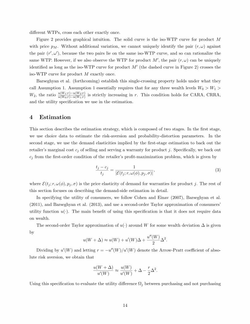
Figure 2 provides graphical intuition. The solid curve is the iso-WTP curve for product M

with price pM . Without additional variation, we cannot uniquely identify the pair (r, ω) against

the pair (r0, ω0), because the two pairs lie on the same iso-WTP curve, and so can rationalize the

same WTP. However, if we also observe the WTP for product M 0, the pair (r, ω) can be uniquely

identified as long as the iso-WTP curve for product M 0 (the dashed curve in Figure 2) crosses the

iso-WTP curve for product M exactly once.

Barseghyan et al. (forthcoming) establish this single-crossing property holds under what they

call Assumption 1. Assumption 1 essentially requires that for any three wealth levels W0 > W1 > u(W1;r)−u(W2;r)W2, the ratio is strictly increasing in r. This condition holds for CARA, CRRA, u(W0;r)−u(W1;r)

and the utility specification we use in the estimation.

Estimation

This section describes the estimation strategy, which is composed of two stages. In the first stage,

we use choice data to estimate the risk-aversion and probability-distortion parameters. In the

second stage, we use the demand elasticities implied by the first-stage estimation to back out the

retailer’s marginal cost cj of selling and serving a warranty for product j. Specifically, we back out

cj from the first-order condition of the retailer’s profit-maximization problem, which is given by

tj − cj 1 = , (3)

tj |E(tj ; r, ω(φ), pj , σ)|

where E(tj ; r, ω(φ), pj , σ) is the price elasticity of demand for warranties for product j. The rest of

this section focuses on describing the demand-side estimation in detail.

In specifying the utility of consumers, we follow Cohen and Einav (2007), Barseghyan et al.

(2011), and Barseghyan et al. (2013), and use a second-order Taylor approximation of consumers’

utility function u(·). The main benefit of using this specification is that it does not require data

on wealth.

The second-order Taylor approximation of u(·) around W for some wealth deviation Δ is given

by 00(W )u

u(W + Δ) ≈ u(W ) + u 0(W )Δ + Δ2 . 2

Dividing by u0(W ) and letting r = −u00(W )/u0(W ) denote the Arrow-Pratt coefficient of abso-

lute risk aversion, we obtain that

u(W + Δ) u(W ) r ≈ +Δ − Δ2 . u0(W ) u0(W ) 2

Using this specification to evaluate the utility difference Ωj between purchasing and not purchasing

14

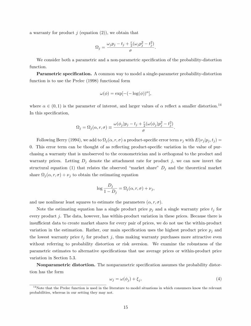
a warranty for product j (equation (2)), we obtain that

. (ωj p − t )j j

We consider both a parametric and a non-parametric specification of the probability-distortion

function.

Parametric specification. A common way to model a single-parameter probability-distortion

function is to use the Prelec (1998) functional form

ω(φ) = exp[−(− log(φ))α],

2

where α ∈ (0, 1) is the parameter of interest, and larger values of α reflect a smaller distortion.14

2

In this specification,

ωj pj − tj + r

σ 2Ωj =

22(ω(φj )p − t )j j

Following Berry (1994), we add to Ωj (α, r, σ) a product-specific error term νj with E(νj |pj , tj ) =

0. This error term can be thought of as reflecting product-specific variation in the value of pur-

chasing a warranty that is unobserved to the econometrician and is orthogonal to the product and

warranty prices. Letting Dj denote the attachment rate for product j, we can now invert the

structural equation (1) that relates the observed “market share” Dj and the theoretical market

share Ωj (α, r, σ) + νj to obtain the estimating equation

Djlog = Ωj(α, r, σ) + νj ,

1 − Dj

and use nonlinear least squares to estimate the parameters (α, r, σ).

Note the estimating equation has a single product price pj and a single warranty price tj for

every product j. The data, however, has within-product variation in these prices. Because there is

insufficient data to create market shares for every pair of prices, we do not use the within-product

variation in the estimation. Rather, our main specification uses the highest product price pj and

the lowest warranty price tj for product j, thus making warranty purchases more attractive even

without referring to probability distortion or risk aversion. We examine the robustness of the

parametric estimates to alternative specifications that use average prices or within-product price

variation in Section 5.3.

Nonparametric distortion. The nonparametric specification assumes the probability distor-

tion has the form

ωj = ω(φj ) + ξj , (4)

Note that the Prelec function is used in the literature to model situations in which consumers know the relevant probabilities, whereas in our setting they may not.

2ω(φj )pj − tj + r

σ Ωj = Ωj (α, r, σ) ≡ .

15

14

5

where φj is the failure probability of product j, ω(·) is some unknown function, and ξj is a product-

specific noise in the probability distortion. We assume the expected value of ξj is zero conditional

on a given failure probability and TV and extended warranty prices in the same subcategory.

Using the same inversion strategy as in Berry (1994) and rearranging, we express the ωj as a

function of the unknown parameters (r, σ) and the data:

σ log Dj + tj + r t2 1−Dj 2 j

ωj = . (5)2pj + 2 r pj

The estimation then proceeds in two steps. We first construct moment conditions involving ωj

and use them to estimate r and σ. We then use the estimated r and σ and the data to back out

the nonparametric estimates of ωj from equation (5).

To construct the moment conditions, we fix a product subcategory, for example, 30” or larger

TVs, and consider two products j and j0 in this subcategory with the same failure probability. The

difference between the respective ω’s is ωj − ωj0 = ξj − ξj0 . Because the expected value of ξ is zero,

we obtain the moment condition

E[ωj − ωj0 |φj = φj0 , pj , pj0 , tj , tj0 ] = 0. (6)

Moreover, because prices are assumed to be orthogonal to the difference between ω’s in the sub-

category, we also obtain the expected value of (ωj − ωj0 )P where P ∈ {pj , pj0 , tj , tj0 } is also zero. Thus, we have five moment conditions. In each of them, we replace the ω’s with the right-

hand side of equation (5) and use the generalized method of moments to estimate r and σ. The

estimation requires that each pair of products we consider is from the same subcategory and shares

the same failure probability. We have 2,040 such pairs in the data.

Results

This section reports the estimates of the probability-distortion function, the risk-aversion parame-

ter, and the seller’s cost.

5.1 The relevance of probability distortions

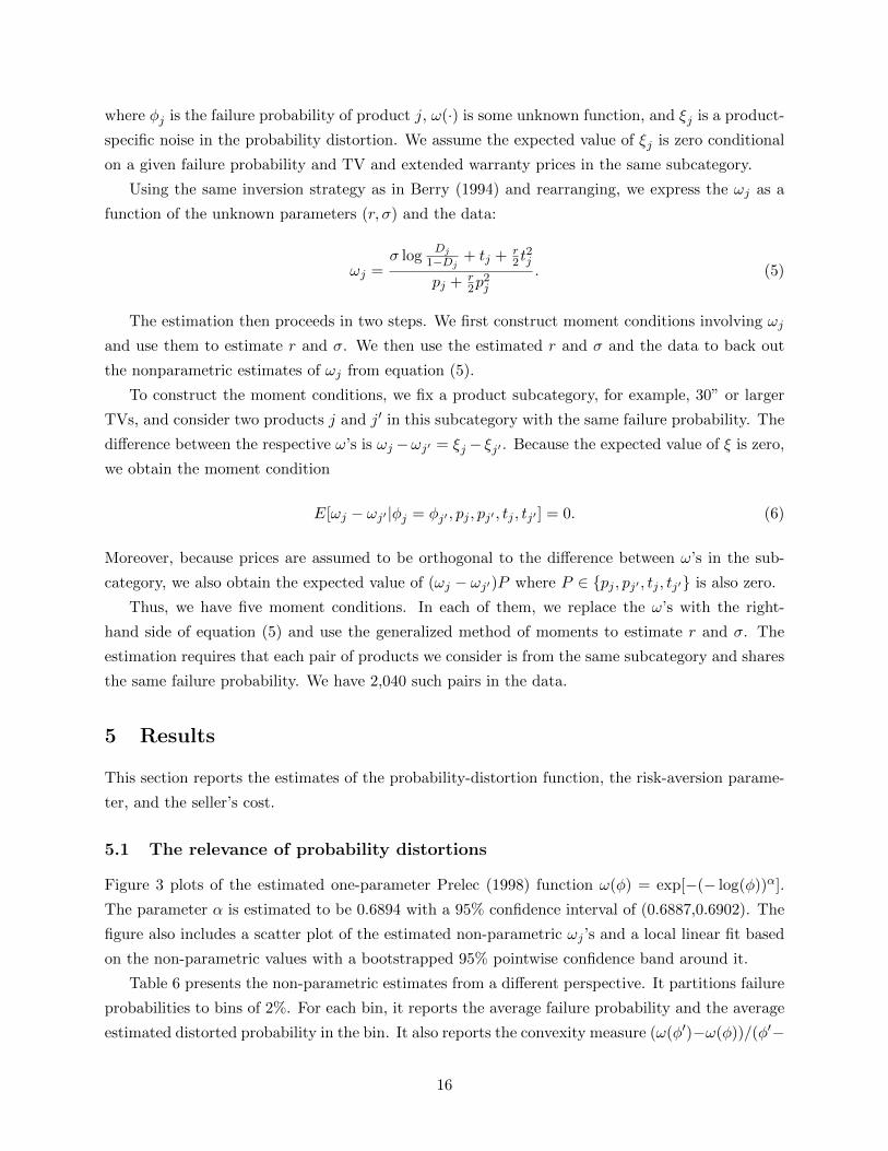
Figure 3 plots of the estimated one-parameter Prelec (1998) function ω(φ) = exp[−(− log(φ))α].

The parameter α is estimated to be 0.6894 with a 95% confidence interval of (0.6887,0.6902). The

figure also includes a scatter plot of the estimated non-parametric ωj ’s and a local linear fit based

on the non-parametric values with a bootstrapped 95% pointwise confidence band around it.

Table 6 presents the non-parametric estimates from a different perspective. It partitions failure

probabilities to bins of 2%. For each bin, it reports the average failure probability and the average

estimated distorted probability in the bin. It also reports the convexity measure (ω(φ0)−ω(φ))/(φ0−

16

Table 6: Estimates of probability distortion

Fail prob intervals Average fail prob Average distorted prob Convexity measure 4–6 5.0 13.5 — 6–8 6.8 16.5 1.7 8–10 9.3 17.5 0.4 ≥10 13.4 17.9 0.1

Notes: Columns 1,2, and 3 are in %. In column 1, the upper bound is not included in the bin.

φ), where φ0 > φ are two adjacent average failure probabilities in the table. This convexity measure

is the increment in the average distortion divided by the increment in the average failure probability.

Two patterns emerge in Figure 3 and Table 6. First, there is substantial upward distortion of

failure probabilities. This is illustrated in Figure 3 by the estimated Prelec function, most of the

estimated wj ’s, the local linear fit, and the 95% confidence band, all lying above the 45-degree line.

This is also illustrated in Table 6 where, for example, products with an average failure probability

of 5% are perceived as products with a 13.5% failure probability. Second, the degree of the upward

distortion decreases as the failure probability increases. This is illustrated in Figure 3 by the

concavity of the local linear fit, and in Table 6 by the decrease in the convexity measure. These

two patterns are in line with the findings of Barseghyan et al. (2013).

5.2 The irrelevance of risk aversion

The estimate of the risk-aversion parameter r is close to zero in both the parametric and non-

parametric specifications of the distortion function. In both specifications, it is less than 10−6 and

is not statistically different from zero.

To interpret the relative importance of the estimated parameters, Table 7 presents the implied

WTP for an extended warranty to a TV that costs $400 under various failure probabilities.15

In column 2, we calculate WTP with the estimated one-parameter distortion function and the

estimated risk-aversion parameter. In column 3, we calculate WTP using the same risk-aversion

parameter while imposing ω(φ) = φ. The comparison of WTPs across the two columns indicates

the contribution of probability distortion to WTP is significantly larger than that of standard risk

aversion. Moreover, when the probability distortion is turned off (column 3), WTP is essentially

equal to the actuarially fair rate.

The estimation “favors” the probability distortion explanation over the risk-aversion explana-

tion, because probability distortion implies — in line with the data — smaller variations in WTP

in response to variations in repair cost than the variations in WTP implied by risk aversion. To

see this, consider a situation in which the repair cost increases at a constant rate while the failure

probability remains fixed. Probability distortion without risk aversion implies WTP increases at

a constant rate, whereas risk aversion without probability distortion implies WTP increases at an

increasing rate. For example, if the failure probability is 5%, the repair cost is $400, and the WTP

15In calculating WTP, all the error terms are set to zero.

17

Table 7: WTP for EW on a good that costs $400

Failure prob Model estimates Model estimates imposing ω(φ) = φ in WTP calculation

0.04 42.63 16.00 0.06 51.99 24.00 0.08 60.18 32.00 0.10 67.65 40.00 0.12 74.63 48.00 0.14 81.26 56.00

for a warranty is $60, then the WTP can be explained by either ω = 0.15 and no risk aversion or

by r = 0.018 and no probability distortion. As the repair cost increases, the WTP in the model

with probability distortion increases at a constant rate of ω. So if the repair cost increases to $500,

WTP increases to $75, and if the repair cost increases to $600, WTP increases to $90. The WTP

in the model with risk aversion increases at a faster rate. If the repair cost increases to $500, WTP

increases to $79, and if the repair cost increases to $600, WTP increases to $101. Thus, although

either probability distortion or risk aversion can explain the WTP for a single product, the rate at

which WTP changes in response to a change in the repair cost favors probability distortion.

Another source of variation that favors probability distortion over risk aversion is the variation

in WTP in response to changes in failure probability. Recall that we assume in the parametric

specification — and infer from the estimates in the non-parametric specification — that the distor-

tion function is concave for the relevant range of failure probabilities. Now consider a situation in

which the repair cost is fixed and the failure probability increases at a constant rate. Probability

distortion without risk aversion implies WTP increases at a decreasing rate, whereas risk aversion

without probability distortion implies WTP increases at a constant rate. Thus, similar to the repair

cost, the slower rate at which WTP changes in response to changes in the failure probability in the

data favors probability distortion.

5.3 Robustness of demand-side estimates

The estimates of the probability-distortion and risk-aversion parameters are robust to the following

alternative specifications (see Tables 8 and 9 for a comparison of the parameter estimates across

specifications.)

Average prices. The main specification uses the highest product price and the lowest warranty

price in the estimation.

We reestimate the parametric model using the average product and warranty prices. It is

expected that the estimated parameters will reflect either a larger probability distortion (smaller

α) or more aversion to risk (larger r) relative to the main specification, because warranty purchases

become less attractive as warranty prices increase or product prices decrease.

Table 8 demonstrates that the estimated distortion parameter α is indeed smaller than in the

18

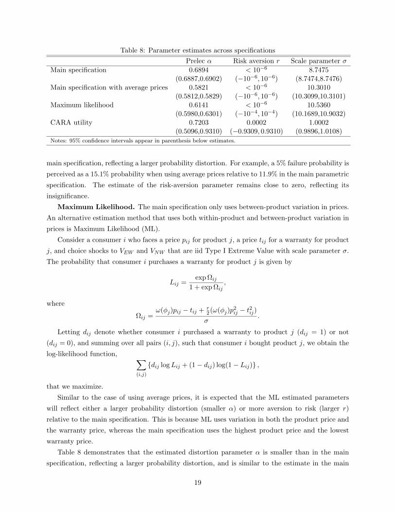
Table 8: Parameter estimates across specifications

Prelec α Risk aversion r Scale parameter σ Main specification 0.6894 < 10−6 8.7475

(0.6887,0.6902) (−10−6 , 10−6) (8.7474,8.7476) Main specification with average prices 0.5821 < 10−6 10.3010

(0.5812,0.5829) (−10−6 , 10−6) (10.3099,10.3101) Maximum likelihood 0.6141 < 10−6 10.5360

(0.5980,0.6301) (−10−4 , 10−4) (10.1689,10.9032) CARA utility 0.7203 0.0002 1.0002

(0.5096,0.9310) (−0.9309, 0.9310) (0.9896,1.0108) Notes: 95% confidence intervals appear in parenthesis below estimates.

main specification, reflecting a larger probability distortion. For example, a 5% failure probability is

perceived as a 15.1% probability when using average prices relative to 11.9% in the main parametric

specification. The estimate of the risk-aversion parameter remains close to zero, reflecting its

insignificance.

Maximum Likelihood. The main specification only uses between-product variation in prices.

An alternative estimation method that uses both within-product and between-product variation in

prices is Maximum Likelihood (ML).

Consider a consumer i who faces a price pij for product j, a price tij for a warranty for product

j, and choice shocks to VEW and VNW that are iid Type I Extreme Value with scale parameter σ.

The probability that consumer i purchases a warranty for product j is given by

exp ΩijLij = ,

1 + expΩij

where 2 − t2ω(φj )pij − tij + r

2 (ω(φj )pij ij )Ωij = .

σ

Letting dij denote whether consumer i purchased a warranty to product j (dij = 1) or not

(dij = 0), and summing over all pairs (i, j), such that consumer i bought product j, we obtain the

log-likelihood function, X {dij log Lij + (1 − dij ) log(1 − Lij )} ,

(i,j)

that we maximize.

Similar to the case of using average prices, it is expected that the ML estimated parameters

will reflect either a larger probability distortion (smaller α) or more aversion to risk (larger r)

relative to the main specification. This is because ML uses variation in both the product price and

the warranty price, whereas the main specification uses the highest product price and the lowest

warranty price.

Table 8 demonstrates that the estimated distortion parameter α is smaller than in the main

specification, reflecting a larger probability distortion, and is similar to the estimate in the main

19

specification with average prices. The estimate of the risk-aversion parameter remains close to zero,

as in the other specifications.

CARA utility. The main specification uses a second-order Taylor approximation of the utility

function. An alternative specification that does not require data on wealth is CARA:

1 − exp(−r(W + Δ)) u(W +Δ) = .

r

We reestimate the model with this alternative specification using the highest product price and

the lowest warranty price. As Table 8 indicates, we obtain a value of α that is similar to the main

specification, and a risk-aversion parameter that is not statistically different from 0.

Repair cost. The utility from not buying a warranty, VNW , depends on the distribution of the

repair cost X. The main specification assumes away this dependence by bounding X from above

with the main product price, thus making the purchase of a warranty more attractive without refer-

ring to risk aversion or probability distortion. However, this assumption may affect the estimates

of the probability-distortion and risk-aversion parameters differently. We now consider alternative

cost specifications to verify this is not the case.

Assume the repair cost X is distributed on the interval [0, p], where p is the main product price.

Without loss of generality, let X be equal to κp, where κ is a random variable with support in

[0, 1]. Using the second-order approximation of consumers’ utility, we can write VNW as a function

of the first two moments of the repair-cost distribution (ignoring the constant term u(W )):

r VNW = ω(φ)pE(κ) + ω(φ)p 2[V ar(κ) + E(κ)2].

2

Thus, knowing the mean and variance of κ is sufficient to compute the utility difference Ω.

Letting µ denote the expected value of κ, the variance σ2 of κ is bounded above by µ(1 − µ)µ

because κ is distributed on [0, 1] and the largest variance is obtained when the probability mass

is concentrated at the end points of the interval. Thus, to check the robustness of the estimates

to the cost specification, it suffices to re-estimate the model for all combinations of µ ∈ [0, 1] and

σ2 µ ∈ [0, µ(1 − µ)].

We find that across all combinations of mean and variance, the effect of the variance on the

parameter estimates is negligible, suggesting that it suffices to examine specifications in which

consumers perceive the repair as a deterministic fraction of the product price. Table 9 reports the

estimates of the probability-distortion and risk-aversion parameters for various fractions. As the

table shows, when the repair cost decreases and thus purchasing a warranty becomes less attractive,

the estimated magnitude of the distortion increases, but the risk-aversion parameter continues to

be irrelevant.

20

Table 9: Parameter estimates with varying repair cost

% of product price Prelec α Risk aversion r ω(0.05) 100% 0.689 < 10−6 0.119 90% 0.639 < 10−6 0.133 80% 0.579 < 10−6 0.151 70% 0.507 < 10−6 0.175 60% 0.416 < 10−6 0.206 50% 0.297 < 10−6 0.250 40% 0.128 < 10−6 0.316 30% 0 0.0339 0.368

Notes: The Prelec parameter is constrained to be weakly greater than 0. This constraint binds between 30% and 40%.

5.4 Retailer’s cost

Figure 4 presents a scatter plot of the non-parametric cost estimates divided by the corresponding

TV prices, and a local linear fit with a bootstrapped 95% confidence band.

For the purpose of the counterfactual analysis, we also fit the non-parametric cost ratios with

the polynomial µ0 + µ1φ + µ2φ2 . As Figure 4 illustrates, the fitted polynomial 0.04+1.32φ − 2.48φ2

is essentially identical to the local linear fit. Using the quadratic fit, we estimate that the retailer’s

cost, which includes commissions to sales people and revenue sharing with warranty providers, is

about 54% of the price of the warranty and that the retailer’s profit margin is about 46%.

5.5 Model fit

We examine how well the model and the estimates fit the data by comparing attachment rates and

warranty prices predicted by the model to those in the data. The prices used in the comparison are

the ones used in the main specification, namely, the highest product price and the lowest warranty

price.

To compute predicted attachment rates at the product level, we plug into equation (1) the non-

parametric estimate of the probability-distortion function, the estimated risk-aversion and scale

parameters, and the observed TV and warranty prices from the data. The model predicts a mean

attachment rate of 0.276, which is similar to the 0.268 mean attachment rate in the data. Figure 5

depicts that the distributions of the predicted and observed attachment rates are also similar.

To compute the predicted warranty prices, we construct the demand for warranties at the

product level based on the non-parametric estimates of the distortion function, estimated risk-

aversion and scale parameters, and the observed TV prices from the data. Using this demand and

the non-parametric cost estimate, we derive the retailer’s profit-maximizing warranty price.

The model predicts a mean warranty-to-product price ratio of 0.175, which is similar to the 0.171

price ratio in the data.16 Figure 6 depicts that the distributions of the predicted and observed price

16Note these price ratios are smaller than the 0.223 price ratio in Table 2 because of the choice of observed prices.

21

6

ratios are also similar.

What Drives Probability Distortions?

This section studies the mechanism for the upward distortion of failure probabilities, an important

step in evaluating consumer welfare and various policy tools that aim to improve consumer welfare.

One possible mechanism is misperception of unknown probabilities. Uninformed consumers

overestimate failure probabilities, and hence are willing to pay for warranties more than they

would if they knew these probabilities. Another possible mechanism is overweighting of known

small probabilities. Prospect Theory (Kahneman and Tversky (1979)) proposes that individuals

incorporate probabilities in decision making by using decision weights, and in particular, assign

high decision weights to low probability events. Of course, a combination of the two mechanisms

might also drive the distortion.

We use a pretest and two main experiments to study the mechanism. The pretest elicits TV

failure rates in the population of participants. The first main experiment elicits the WTP for

warranties of uninformed participants, who do not receive information about the failure rate from

the pretest, and informed participants, who do. It also elicits the perceived failure probability of

uninformed participants. The main takeaway from this experiment is that uninformed participants

overestimate failure probabilities, and that their WTP is much higher than the WTP of informed

participants.

The second main experiment studies whether informed participants distort failure probabilities,

an indication for probability overweighting. It elicits informed participants’ WTP for warranties for

different TVs with the same failure rate, and uses the empirical strategy of Section 4 to estimate

the degree of probability distortion and standard risk aversion post information provision. The

main takeaway from this experiment is that there is a mild distortion of failure probabilities post

information provision.

In all experiments, we use the Mechanical-Turk (M-Turk) platform. We recruited participants

who performed at least 500 tasks on M-Turk prior to each experiment, and had an approval rating

of 90% or more. About 56% of the participants were males, 43% were females, and 1% preferred

not to specify their gender. The median age bracket in the sample was 25-34 years and the median

household annual income bracket was $40,000-49,999. The distributions of age and household

income brackets appear in Figure 7. Each participant participated in one experiment and was

randomly assigned to one treatment in the experiment.

6.1 Pretest

This experiment elicits failure rates in the population of participants.

Participants (N = 504) were invited to participate in an experiment about TVs. We expected

the experiment would take up to two minutes to complete and promised a payment of 25 cents for

22

Table 10: TV Repair rates

2015 2016 2017 Average # Bought 193 206 116 — # Needed repair 8 12 5 — Implied fail rate 4.1% 5.8% 4.3% 4.9%

participation.

We first asked participants if they had bought a TV in the past three years. Those who

responded positively were asked to report, for each TV they bought, the year they bought it (2015,

2016, or 2017)17 and whether it had needed a repair by a technician.

About 72% of the participants reported they had bought a TV in the past three years. From

among them, about 64% reported they had bought one TV, 28% that they had bought two TVs,

and the rest three or more.

Table 10 reports that failure rates across years range between 4% and 6%, and that the average

failure rate is 4.9%. This number is similar to the failure rates in Consumer Reports. Consumer

Reports surveyed the performance of 23 major TV brands in early 2017 based on a sample of more

than 100,000 TV owners between 2011 and 2016. The mean and the median three-year failure rates

by brand are 5%, with 17 out of the 23 brands having a failure rate of 2% to 5%, 5 brands having

failure rates of 6% to 7%, and the remaining brand (Spectre) having a failure rate of 10%.

6.2 Experiment 1

This experiment elicits the WTP for warranties of uninformed participants, who do not receive

information about the failure rate from the pretest, and informed participants, who do. It also

elicits the perceived failure probability among uninformed participants.

We expected the experiment would take up to three minutes to complete, and promised a

payment of 40 cents for participation.

At the beginning of the experiment, participants (N=1001) were asked to “Imagine you just

bought a TV for $600. The TV is by LG, and has a 50” screen and Ultra HD technology.”18 They

were then randomly assigned to one of three treatments.

In the first treatment, denoted Treatment WTP-First, participants were asked to complete the

following sentence:

“The maximum amount in dollars that I am willing to pay for a protection plan that will cover

all the repair costs of this TV in the next three years is ”.

They were then asked: “In your opinion, what is the likelihood in percentages (%) that this TV

will need a repair in the next three years?”.

17The experiment was conducted in mid-October 2017. 18LG is one of the brands with a 5% failure rate according to Consumer Reports. We selected the TV attributes

and price based on online offerings at BestBuy and Costco at the time of the experiment.

23

We incentivized the second question by promising participants 10 additional cents if their re-

sponse was among the 10 most accurate responses.

In the second treatment, denoted Treatment Likelihood-First, the order of the questions was

reversed.

In the third treatment, denoted Treatment Information-First, participants were first informed

that “You are told by an expert friend that the likelihood the TV will need a repair within the

next three years is 5%.”

They were then asked to report the maximum amount they would be willing to pay for a

three-year protection plan, as in the other treatments.

After completing one of the three sets of questions above, participants were asked several ques-

tions about the TVs they bought in the past few years. They then reported their age bracket,

income bracket and gender.

First finding: Failure probabilities are overestimated. The mean perceived failure prob-

abilities in treatments WTP-First and Likelihood-First are 13.49% (standard error of 0.81) and

15.12% (standard error of 0.86) respectively. The median perceived probability in both treatments

is 10%. These numbers are much higher than the objective three-year failure rate reported above.

Thus, uninformed participants overestimated the failure probabilities. Moreover, the magnitude of

the overestimation as reflected in the mean perceived probability is similar to that of the empirical

analysis, in which a 5% failure probability is perceived as 11.9% in the parametric specification and

13.5% in the non-parametric specification.

Figure 8 provides a finer description of the perceived probabilities by means of Cumulative

Distribution Functions (CDFs). For each treatment, the CDF assigns for every 0 ≤ x ≤ 100 the

proportion of participants in the treatment who estimated the failure probability to be weakly less

than x%. The CDFs are similar (the Kolmogorov–Smirnov (KS) test statistic for the equality of

the CDFs is 0.086 (p = 0.151)). In each of them, more than 60% of the participants reported

probabilities that were at least two-fold larger than the objective probability.

To examine the robustness of the reported probabilities to changes in incentives, we re-ran the

two treatments with a smaller group of 209 participants. We promised participants a bonus of 20

cents, which is twice as large as the original incentive, if their estimate was among the 10 most

accurate ones.

We find no significant difference in the reported probabilities relative to a bonus of 10 cents.

The mean reported probability is 14.28 (standard error of 1.39) in Treatment WTP-First and

16.36 (standard error of 1.78) in Treatment Likelihood-First. The two CDFs of Treatment WTP-

First with 10-cent and 20-cent incentives are similar (p = 0.36), as are the two CDFs of Treatment

Likelihood-First (p = 0.50). Thus, the reported probabilities are robust to this change in incentives.

24

Table 11: WTP with and without information

Treatment WTP-First (N = 334) Likelihood-First (N = 330) Information-First (N = 337)

Mean WTP 73.01 (5.88) 53.69 (2.68) 42.73 (4.15) Mean WTP truncated 64.35 (3.96) 47.84 (1.96) 36.33 (2.66) Median WTP 50 50 25 Note: Standard errors in parenthesis. Second row mean is truncated to eliminate the top one percentile of the WTP distribution.

Second finding: WTP drops when information is provided. Table 11 summarizes partici-

pants’ reported WTP for a three-year warranty across treatments. The mean and the median WTP

in Treatment Information-First are significantly smaller than in Treatment WTP-First, indicating

that providing participants with information about the objective failure rate reduced their WTP

significantly. Stronger evidence for this assertion is given in Figure 9, which draws the CDFs of

the WTP distributions by treatment. The CDF for Treatment Information-First essentially first-

order-stochastically dominated by the CDF for Treatment WTP-First, indicating that WTP for

warranties was reduced with information (the KS statistic for the equality of the CDFs is 0.309

(p < 0.001)).

Two forces are potential drivers of the reduction in WTP. First, Treatment Information-First

reminded participants about failure probabilities prior to reporting WTP. Merely reminding partic-

ipants about failure probabilities (independently of whether the objective probability was specified

or not) prior to reporting WTP could have driven the reduction in WTP. Second, Treatment

Information-First informed participants about the objective failure probability. It is possible that

informing participants about this low probability is what drove the reduction in WTP. To exam-

ine the relevance of these two forces, we compare the WTP in Treatment Likelihood-First with

the WTP in treatments WTP-First and Information-First because the first force (i.e. reminder

about probabilities) but not the second force ( i.e. information provision) was present in Treatment

Likelihood-First.

The data provides strong evidence for the presence of the second force. The CDF for Treatment

Information-First in Figure 9 is essentially first-order stochastically dominated by the CDF for

Treatment Likelihood-First (the KS statistic is 0.238 (p < 0.001)). The mean and median WTPs

are also significantly different.

There is also suggestive evidence for the presence of the first force. The mean WTP in Treatment

Likelihood-First is significantly lower than in Treatment WTP-First (p = 0.0018). The CDF for

Treatment Likelihood-First in Figure 9 also appears to be first-order stochastically dominated by

the CDF for Treatment WTP-First, however, this is not statistically significant (the KS statistic

is 0.087 (p = 0.14)). A possible explanation of the substantial difference in the mean WTP but

not in the WTP distribution, which is also supported by examining the truncated mean WTP in

Table 11, is that reminding participants about probabilities has a larger effect on participants with

higher WTP.

25

6.3 Experiment 2

This experiment elicits the WTP of informed participants for warranties for different TVs with

the same failure rate, and uses the empirical strategy of Section 4 to estimate participants’ proba-

bility distortion and standard risk aversion post information provision. The estimated probability

distortion of informed participants can then be interpreted as reflecting probability overweighting,

and the gap between the estimated distortion and the perceived failure probabilities of uninformed

participants in Experiment 1 as reflecting probability overestimation.

We expected the experiment would take up to three minutes to complete, and promised a

payment of 40 cents for participation.

Participants (N = 916) were randomly assigned to one of two treatments. In the first treatment,

denoted Treatment 600-TV, participants were asked to “Imagine you just bought a TV for $600.

The TV is by LG, and has a 50” screen and Ultra HD technology.” That is, the specification of

the TV was identical to the one in Experiment 1.

In the second treatment, denoted Treatment 1000-TV, participants were first asked to “Imagine

you just bought a TV for $1000. The TV is by LG, and has a 70” screen and Ultra HD technology.”

That is, the TV price was higher than in Treatment 600-TV, and to make sure the $1000 price was

realistic, the screen size was also larger.

As in Treatment Information-First in Experiment 1, participants in both treatments were then

informed about the 5% objective failure rate, and were asked to report the maximum amount they

would be willing to pay for a three-year protection plan.

After answering the first question, participants were asked whether they had bought a TV in

the past three years, and reported their age bracket, income bracket, and gender.

Preliminary finding: WTP changes significantly with price. Participants’ WTP for war-

ranties is much higher for $1000 TVs than for $600 TVs. The mean WTP is 66.22 (standard error

of 3.96) in Treatment 1000-TV relative to 46.89 (standard error of 3.43) in Treatment 600-TV, and

the median WTP is 50 relative to 25. Figure 10 illustrates this ranking extends to the CDFs as the

CDF for $1000 TVs first-order stochastically dominates the CDF for $600 TVs (the KS statistic

for the equality of the CDFs is 0.199 (p < 0.001)).

Main finding: Probability distortions are significantly reduced when information is

provided. After truncating the top one percentile of the WTP distribution, we use the empirical

strategy of Section 4 to estimate the degree of probability distortion and standard risk aversion

among participants under two scenarios.

In the first scenario, we assume participants share the same distortion w and the same risk-

aversion parameter r, but may differ from one another in various unobserved factors. As a result,

participants’ reported WTP does not equate the utility difference Ω to 0 precisely. Rather, it

equates Ω to an error parameter �, which is equal to 0 in expectation. We estimate this model

26

using nonlinear least squares to find r and w.

The estimated value of w is 6.3%, which implies a 1.3% distortion of the objective probability.

This distortion is about one-seventh of the 8.9% distortion expressed by uninformed participants

in Experiment 1.19 The estimate of the risk-aversion parameter is negligible.

In the second scenario, we divide participants into quartiles based on their WTP. We match

the corresponding quartiles across treatments, and assume participants in each combined quartile

share the same w and r. We repeat the above estimation procedure for each quartile separately.

We find that neither risk aversion nor probability distortions is required to explain WTP of the

lower half of the WTP distribution. The estimated value of w for the 50-75 quartile is 7.1%, which

implies a 2.1% distortion. This distortion is much smaller than the upward distortion of about

9.5% among the 50-75 quartile in Experiment 1. The 75-100 quartile has an upward distortion

of 8.0%, which is again much smaller than the 28.4% distortion for the corresponding quartile in

Experiment 1.

Thus, providing information to participants reduces probability distortions significantly. Be-

cause the distortion post information provision provides an upper bound on the degree of probabil-

ity overweighting, we conclude that the role of overweighting in driving participants’ WTP is not

significant once they become informed about the objective failure probability.

6.4 Discussion

The experimental results indicate that providing information about objective failure probabilities

reduces WTP significantly. A primary driver of the reduction in WTP is that information provi-

sion reduces overestimation. Indeed, the estimated failure probability of informed participants in

Experiment 2 is (1) much smaller than the average perceived failure probability in Experiment 1,

and (2) similar to the objective failure probability elicited in the pretest. This latter observation

also indicates the insignificant role of probability overweighting post information provision.

There is also suggestive evidence that merely prompting participants to think about failure

probabilities prior to reporting WTP reduces their WTP. One possible explanation for the reduction

in WTP is that prompting participants to think about relevant aspects of the value of the warranty

enhances their decision making. Another possible explanation, following the Bordalo et al.’s (2015)

theory of attention, is that people are surprised when the unlikely event of TV failure is first

mentioned to them and overreact to this information when reporting WTP (Treatment WTP-First).

As the surprise element is reduced, participants report lower WTP (Treatment Likelihood-First).20

Testing these and other possible explanations for why promoting participants to think about failure

19We truncate the top one percentile of the WTP distribution in Experiment 1 for the purpose of this comparison. 20The surprise element may also explain why the magnitude of the probability distortion in Experiment 2 is small

relative to what is documented in the experimental literature (see e.g. Fehr-Duda and Epper (2012) for a survey.) Participants may be surprised when they realize — following information provision in Experiment 2 — that the objective failure probability is much smaller than they initially thought, and respond to this surprise by reporting a more conservative WTP.

27

7

probabilities reduces their WTP is a task for future research.

The Effect of Probability Distortions on Economic Outcomes

This section uses counterfactual analysis to quantify the effect of probability distortions relative to

market power on economic outcomes.

We consider four scenarios in the analysis. The first scenario, “Market power with Biased

consumers”(scenario MB), corresponds to the existing market in which the retailer has monopolist

market power and buyers distort failure probabilities. In the second scenario, “Market power with

Unbiased consumers” (scenario MU), the retailer continues to benefit from the same market power

but buyers do not distort failure probabilities. Comparing the second scenario with the first enables

us to study the importance of probability distortions while fixing the existing market environment.

In the third scenario, “Competitive market with Unbiased consumers” (scenario CU), unbiased

consumers purchase warranties in a competitive market. Because of competition, market prices are

equal to the retailers’ marginal cost and retailers make zero profit. Comparing this scenario with the

second scenario enables us to study the importance of market power in the absence of probability

distortions. In the fourth scenario, “Competitive market with Biased consumers” (scenario CB),

retailers price at marginal cost and buyers distort failure probabilities. Comparing this scenario

with scenario CU enables us to study the importance of probability distortions in a counterfactual

competitive environment.

We assume that any change in the main product’s price across the four scenarios is negligible.

To motivate this assumption, we first observe that little differentiation exists between electronics

retailers, and that TV prices are easily observable. Thus, in the absence of extended warranties and

other add-ons, TVs would have been priced close to marginal cost. The introduction of extended

warranties implies retailers may have incentives to cut TV prices below cost in order to increase

the demand for warranties.

There are several reasons to believe such price cutting, if it happens, is insignificant. First,

on the theoretical side, Ellison’s (2005) analysis indicates the incentive to cut prices below cost is

mitigated by an “adverse selection” effect, i.e., cutting TV prices will attract a disproportionate

volume of consumers with low WTP who will not buy warranties. Second, on the institutional side,

TV manufacturers have tight controls on the pricing and marketing practices of retailers in order

to prevent such price cutting. Two examples of controls are the Minimum Advertised Price (MAP)

policy, whereby retailers cannot advertise below the manufacturer’s suggested retail price, and the

Unilateral Manufacturer’s Retail Price (UMRP) policy, which imposes a penalty when retailers set

prices below the UMRP. Third, on the empirical side, we hand collected and compared 40 TV prices

from BestBuy and Target in 2003. BestBuy offered extended warranties in 2003, whereas Target

did not. To the extent that Target and BestBuy face similar TV wholesale prices, we would expect

TV prices at BestBuy to be lower than at Target if BestBuy’s warranty business affected their

28

TV pricing. We find, however, that TV prices are very similar across retailers. On average, TV

prices at BestBuy are 0.4 percentage points higher than at Target (standard error of 0.9 percentage

points), and the median price difference is 0.

In the four counterfactual scenarios, cost and demand for warranties depend on the TV price p

and the failure rate φ. We use the average TV price of $400 and consider the failure rates {0.04, 0.05, . . . , 0.15}. For the cost specification, we use the parametric estimate of c(pj , φ) with pj = 400.

To construct demand in scenarios MB and CB, we use the estimated α and r from the parametric

estimation. In the two other scenarios, we turn off the distortion by setting ω(φ) = φ but keep the

same r.

7.1 Prices, volume, and profit

Given cost and demand, we calculate optimal prices, attachment rates, and profit margins in the

different scenarios. To derive a yearly dollar equivalent measure of profit, we assume 30 million

people buy TVs every year.21

Panel A in Figure 11 plots the warranty-to-TV price ratio as a function of failure probabilities

for the different scenarios. The price ratios are increasing and concave in the failure probability.

They are highest in scenario MB, lower in scenario MU, and lowest in scenarios CU and CB. The

gap between scenarios MB and MU is smaller than the gap between scenario MU and the two

competitive market scenarios CU and CB.

Thus, probability distortions lead to a price increase, but this price increase is smaller than the

price increase due to market power. For example, at the average failure rate of 7%, the price ratio

in scenario MB is about 20% higher than in scenarios CU and CB. About three quarters of this gap

is attributed to market power (the gap between MU and the competitive-market scenarios), and

the rest to probability distortions. Because prices in the competitive-market scenarios are equal to

marginal cost (which includes payments to third-party providers), the same conclusion applies to

profit margins: pricing power is responsible for three quarters of retailers’ margin.

Panel B in Figure 11 plots attachment rates as a function of failure probabilities. Attachment

rates in scenario MB are 30% or larger, whereas attachment rates in scenario MU are around

5%. That is, fixing the existing competitive environment with market power, the introduction

of probability distortions leads to a five-fold or larger increase in volume.22 Attachment rates in

scenario MB are about three times larger than in scenario CU. That is, any rationing that takes

place due to market power is insignificant relative to the volume increase due to the distortion.

Panel C in Figure 11 plots profits as a function of failure rates. More than 90% of retailers’

profit is due to probability distortions.

21This number is somewhat smaller than the yearly TV shipments in the US between 2010 to 2013, which ranged from 37 million to 40 million. (CNN, “With new TVs, size matters,” June 26, 2013).

22The comparison between scenarios CU and CB also highlights the large effect of the distortion on volume while fixing the competitive environment, as volume more than doubles when moving from scenario CU to scenario CB.

29

To sum up, probability distortions drive the strong demand for warranties and the high profits,

whereas market power drives the high prices and margins.

7.2 Consumer and total welfare

Evaluating consumer welfare requires taking a stance as to whether probability distortions are

welfare-relevant in the sense that the distorted probabilities should be part of consumer welfare. We

interpret the results of the experiment, especially those of Experiment 2, as suggesting they should

not, because the results demonstrate that providing information to consumers about objective

failure probabilities triggers most of them to use the objective or slightly distorted probabilities

in their decision making. Put differently, information provision “reveals” that consumers prefer to

use the objective probabilities in decision making. We thus evaluate welfare with respect to the

objective failure probabilities.

Figure 12 plots consumer welfare as a function of failure rates. Consumer welfare is highest

in scenario CU. This is because consumers evaluate failure probabilities correctly and prices are

lowest. Consumer welfare is lower in scenario MU. This is because prices are higher due to retailers’

market power leading to lower attachment rates. In both scenarios, consumer welfare is positive

because only consumers with true WTP above price buy warranties.

Consumer welfare is negative in scenario MB, which is identical to the existing market. Put

differently, consumer welfare would increase if the market for extended warranties did not exist.

This is because probability distortions are sufficiently large, so that any positive surplus generated

by purchases of buyers with true WTP above price is dominated by the decrease in consumer

welfare due to purchases of buyers with true WTP below price.

Consumer welfare is even lower in scenario CB. This is because the increase in consumer welfare

(relative to scenario MB) due to existing consumers paying lower prices and the entry of new

consumers with true WTP above price is dominated by the decrease in consumer welfare due to

the entry of new consumers with true WTP below price buying warranties because of the distortion.

Figure 12 illustrates that the reduction in consumer welfare due to probability distortions in

the existing competitive environment, i.e., the gap between MU and MB, and in the alternative

competitive environment, i.e., the gap between CU and CB, are much larger than the reduction in

consumer welfare due to market power (the gap between CU and MU or the gap between CB and

MB). For example, at a 7% failure probability, consumer welfare increases by $140 million when

moving from MB to CU, and more than 95% of this increase is due to shutting down the distortion,

i.e., due to the transition from MB to MU.

To illustrate the forces at play, consider the two positive welfare effects when moving from

scenario MB to scenario MU (see Figure 13 for a graphical illustration). First, holding the warranty

price fixed, a shift inward of the demand curve occurs when shutting down probability distortions.

Consumers who now forgo buying the warranty are exactly those who overpaid for warranties based

on their true WTP for it, thus increasing consumer welfare. We refer to this effect as the ripoff

30

8

effect. Second, warranty prices go down when shutting down the distortion. Existing buyers pay

lower prices, and new consumers, who estimate failure probabilities correctly, buy warranties. As a

result, attachment rates and consumer welfare increase. We refer to this effect as the price effect.

Figure 14 plots the dollar-equivalent value of the two effects for various failure rates. The ripoff

effect clearly dominates the price effect for all failure rates.

The effect of probability distortions on total welfare is ex-ante ambiguous. The first-best level

of insurance is the one in scenario CU, because all consumers with true WTP above cost are

insured. In scenario MU, there is under-insurance relative to the first-best, because retailers price

warranties above cost, and thus consumers with true WTP above cost but below market prices are

not insured. In scenarios MB and CB, there is over-insurance relative to the first-best, because

consumers with true WTP below cost purchase insurance due to probability distortions. See Figure

15 for a graphical illustration.

Figure 16 plots total welfare as a function of failure rates. Total welfare in scenario MU is larger

than in scenario MB. Put differently, the adverse welfare effect of market power (the gap between

CU and MU) is smaller than the adverse welfare effect of the distortion (the gap between MU and

MB). The adverse welfare effect of the distortion is so large that total welfare in scenario CB is

lower than in all other scenarios.

Conclusion

This paper analyzed the effect of probability distortions on economic outcomes in the extended

warranty market. We established that the distortion is a dominant factor in driving the strong de-

mand and high profit in this market. We also established that when consumers receive information

about failure probabilities, their willingness to pay for warranties reflects a much smaller distortion,

indicating the distortion is a mistake in decision making due to lack of information. We conclude

with a short discussion of the policy implications of these findings.

In its 2003 report, the UK Competition Commission (2003) proposed that electronics retailers

“display the price of an applicable EW (extended warranty) alongside the DEG (domestic electrical

good) in store and in press advertisement and other publicity.” This proposal is an example of a

competition policy that aims to intensify competition and lead to lower prices. But lower prices do

not necessarily increase consumer welfare, because lower prices imply additional consumers with

willingness to pay below price buy warranties due to overestimation. Our findings suggest con-

sumer policies that aim to improve consumers’ decision making may be more effective in increasing

consumer welfare. An example of such policy, which may have an effect similar to the information-

provision treatments in our experiments, is to demand that retailers display the failure probability

of the product next to its price.

To illustrate this point, we return to our counterfactual scenarios. We can think about scenario

MB as corresponding to the existing market, scenario CB as corresponding to the market outcome

31

following a competition policy that eliminates market power, and scenario MU as corresponding to

the market outcome following a consumer policy that eliminates overestimation.

Panel B in Figure 11 illustrates market volume will more than double if warranties are priced

at cost as we move from MB to CB. However, Figure 12 illustrates consumer welfare will decrease.

Total welfare will also decrease, because firms make zero profit in this scenario. On the other hand,

both consumer welfare and total welfare are positive in scenario MU.

Figure 17 provides additional evidence that consumer policies that lead to a reduction — and

not necessarily the elimination — of the distortion are welfare-superior to competition policies that

lead to price reduction. In the figure, we assume TVs are priced at $400, and the failure probability

is 7%.

In solid blue, we plot for every 0 ≤ λ ≤ 1 how consumer welfare (Panel A) and total welfare

(Panel B) change when consumers distort failure probabilities and warranty prices are a convex

combination of competitive prices with weight λ and monopoly prices with weight 1 − λ. As λ

increases, i.e., as the market becomes more competitive, both consumer and total welfare decrease.

In dashed red, we plot how welfare changes when consumers perceive failure probabilities as a

convex combination of the objective probability with weight λ and the distorted probability with

weight 1−λ, and the retailer prices optimally with respect to the resulting demand. Clearly, welfare

increases in λ, and for any λ, welfare is larger than following any price reduction.

Thus, policies that aim to intensify price competition may lead to suboptimal results in markets

with uninformed or biased consumers relative to consumer policies that aim to improve consumers’

decision making.

References

Armstrong, M. (2008), “Interactions between Competition and Consumer Policy,” Competition

Policy International, 4(1), 97–147.

Barseghyan, L., F. Molinari, T. O’Donoghue, and J. C. Teitelbaum (2013), “The Nature of Risk

Preferences: Evidence from Insurance Choices,” American Economic Review, 103(6), 2499–

2529.

Barseghyan, L., F. Molinari, T. O’Donoghue, and J. C. Teitelbaum (Forthcoming), “Estimating

Risk Preferences in the Field”, Journal of Economic Literature.

Barseghyan, L., J. Prince, and J. C. Teitelbaum (2011), “Are Risk Preferences Stable Across

Contexts? Evidence from Insurance Data,” American Economic Review, 101(2), 591–631.

Berry, S. T. (1994), “Estimating Discrete-Choice Models of Product Differentiation,” RAND Jour-

nal of Economics, 25(2), 242–262.

32

Bordalo, P., N. Gennaioli, and A. Shleifer (2015), “Memory, Attention and Choice”, Working

paper.

Chen, T., A. Kalra and B. Sun (2009), “Why Do Consumers Buy Extended Service Contracts,”

Journal of Consumer Research, 36(4), 611–623.

Chiappori, P. A., A. Gandhi, B. Salanie, and F. Salanie (2012), “From Aggregate Betting Data

to Individual Risk Preferences,” Working paper.

Cohen, A. and L. Einav (2007), “Estimating Risk Preferences from Deductible Choice,” American

Economic Review, 97(3), 745–788.

Diamond, P. A. (1971), “A Model of Price Adjustment,” Journal of Economic Theory, 3(2),

156–168.

Ellison, G. (2005), “A Model of Add-On Pricing,” Quarterly Journal of Economics, 120(2), 585–

637.

Ellison, G. and S. F. Ellison (2009), “Search, Obfuscation, and Price Elasticities on the Internet,”

Econometrica, 77(2), 427–452.

Fehr-Duda, H. and T. Epper (2012), “Probability and Risk: Foundations and Economic Implica-

tions of Probability-Dependent Risk Preferences,” Annual Review of Economics, 4, 567–593.

Gandhi, A. and R. Serrano-Padial (2014), “Does Belief Heterogeneity Explain Asset Prices: The

Case of the Longshot Bias,” Review of Economic Studies, 82(1), 156–186.

Huysentruyt, M. and D. Read (2010), “How do People Value Extended Warranties? Evidence

from Two Field Surveys,” Journal of Risk and Uncertainty, 40(3), 197–218.

Jindal, P. (2014), “Risk Preferences and Demand Drivers of Extended Warranties,” Marketing

Science, 34(1), 39–58.

Jullien, B. and B. Salanie (2000), “Estimating Preferences under Risk: The Case of Racetrack

Bettors”, Journal of Political Economy, 108(3), 503–530.

Kahneman, D. and A. Tversky (1979), “Prospect Theory: An Analysis of Decision under Risk,”

Econometrica, 47(2), 263–291.

Kliger, D. and O. Levy (2009), “Theories of Choice under Risk: Insights from Financial Markets,”

Journal of Economic Behavior and Organization, 71(2), 330–346.

Prelec, D. (1998), “The Probability Weighting Function,” Econometrica, 66(3), 497–527.

33

Rubinstein, A. and Y. Salant (2008), “Some Thoughts on the Principle of Revealed Preference,”

In Handbooks of Economic Methodologies (Andrew Caplin and Andrew Schotter, eds.), New

York: Oxford University Press, 115–124.

Rubinstein, A. and Y. Salant (2012), “Eliciting Welfare Preferences from Behavioral Datasets,”

Review of Economic Studies, 79(1), 375–387.

Snowberg, E. and J. Wolfers (2010), “Explaining the Favorite-Long Shot Bias: Is It Risk-Love or

Misperceptions?”, Journal of Political Economy, 118(4), 723–746.

Sydnor, J. (2010), “(Over)insuring Modest Risks,” American Economic Journal: Applied Eco-

nomics, 2(4), 177–199

UK Competition Commission (2003), “Extended warranties on domestic electrical goods: A report

on the supply of extended warranties on domestic electrical goods within the UK – Volumes

1, 2 and 3.”

34

Figures

Figure 1: Histograms of warranty-to-product price ratios

(A) All Products (B) TVs

Figure 2: Identification: Single-crossing of willingness to pay

•

•

r

1

WTP (pM ′ , φ)

1

WTP (pM , φ)

1

(r, ω)

1

(r′, ω′)

1

ω

1

35

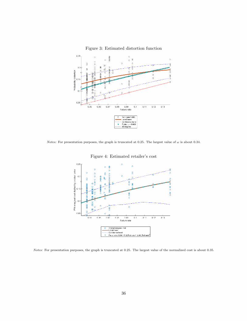
Figure 3: Estimated distortion function

Notes: For presentation purposes, the graph is truncated at 0.25. The largest value of ω is about 0.34.

Figure 4: Estimated retailer’s cost

Notes: For presentation purposes, the graph is truncated at 0.25. The largest value of the normalized cost is about 0.35.

36

Figure 5: Model fit: Attachment rates

Figure 6: Model fit: Warranty-to-TV price ratios

37

Figure 7: Distributions of survey participants

(A) Age (B) Income

Figure 8: CDFs of perceived failure probabilities in Experiment 1

38

Figure 9: CDFs of WTP in Experiment 1

Figure 10: CDFs of WTP in Experiment 2

39

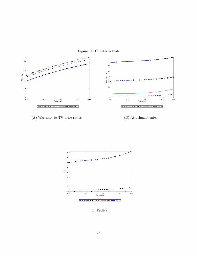
Figure 11: Counterfactuals

(A) Warranty-to-TV price ratios (B) Attachment rates

(C) Profits

40

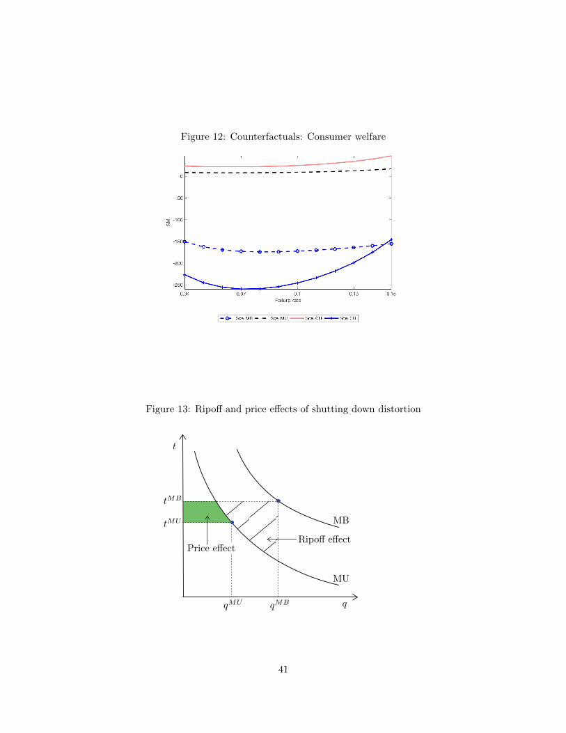
Figure 12: Counterfactuals: Consumer welfare

Figure 13: Ripoff and price effects of shutting down distortion

••

Price effect

1

Ripoff effect

1

MB

1

MU

1

t

1

tMB

1

tMU

1

qMU

1

qMB

1

q

1

41

Figure 14: Counterfactuals: Magnitude of ripoff and price effects

Figure 15: Sources of welfare loss

••

• •

in MU

1

in MB

1

in CB

1

Under-insurance

1

t

1

tMB

1

tMU

1

Welfare loss:

MU relative to CU

1

Welfare loss:

MB relative to CU

1

Demand withdistortion

1

qCB

1

Demand withoutdistortion

1

MC

1

qMU

1

qMB

1

q

1

qCU

1

Over-insurance

1

Welfare loss:

CB relative to MB

1

42

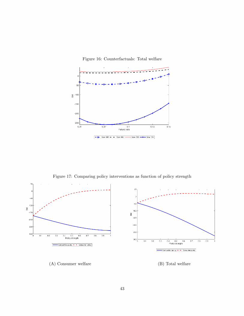
Figure 16: Counterfactuals: Total welfare

Figure 17: Comparing policy interventions as function of policy strength

(A) Consumer welfare (B) Total welfare

43