Micromechanical Modeling and Design Optimization of

2-D Triaxial Braided Composites

John T. Hwang ∗ , Anthony M. Waas † , Joaquim R. R. A. Martins ‡

University of Michigan, Ann Arbor, Michigan, 48109, United States

A micromechanical model for 2-D triaxial braided composites is presented. The tow ar-rangement in the representative unit cell is modeled by solving the packing problem usinganalytical optimization, avoiding the need to measure the geometric properties experimen-tally. These results are used in the development of a closed-form micromechanical modelpredicting the full 3-D stiffness matrix of the homogenized representative unit cell. Theresults show good agreement with experimental data; however, the true significance of thiswork is that it enables design optimization using 2-D triaxial braided composites becausethe need for experimental calibration for each set of design variables is eliminated.

Nomenclature

F∗ {x∗, y∗, z∗}T Plate frameF {x, y, z}T Unit cell frameF ′ {x′, y′, z′}T In-plane tow frameF ′′ {x′′, y′′, z′′}T Undulated tow frameAa,Ab Tow area

Aa,Ab Tow area projected along the other towda,db Tow diameter (major axis)

da,db Tow diameter (major axis) projected along the other towh Plate thicknessH Unit cell heightLa,Lb Tow undulation wavelengthL Unit cell lengthta,tb Tow thickness (minor axis)ua,ub Tow undulation heightVf Fiber volume fraction (fiber to tow)Vt Tow volume fraction (tow to RUC)V ,Vm Total, matrix volumesVa,Vb Tow volumesW Unit cell half-widthα In-plane tow rotation angleβ Undulation angleθ Bias tow angleφ Unit cell orientation angleSubscripta Axial towb Bias towm Matrixt Tow

∗PhD Candidate, Department of Aerospace Engineering.†Professor, Department of Aerospace Engineering.‡Associate Professor, Department of Aerospace Engineering.

1 of 12

American Institute of Aeronautics and Astronautics

I. Introduction

In aircraft design, aeroelastic tailoring is the application of passive control in the design of the structureto produce favorable deformations through the use of directional stiffness.1 When this is achieved, there is asynergistic coupling between aerodynamics and structures that contributes to overall performance benefits.The application of aeroelastic tailoring to wing design has been considered for decades, and studies in theliterature show varying degrees of success, with most making use of composite materials.

Librescu and Song2 were one of the first to apply aeroelastic tailoring to composite wings by varying plyangles in thin-walled composite beams. The additional flexibility in transverse shear from using compositematerials amplified the wash-in effects of forward sweep, which was found to contribute to the impact ofaeroelastic tailoring on the divergence speeds of forward swept wings. Eastep et al.3 performed aeroelastictailoring with strength and flutter constraints on wings modeled with composite skins. They used [0◦, 90◦,±45◦] laminates and optimized the relative proportions of each ply for a range of layup orientations. Theirconclusion was that the effect of aeroelastic tailoring in this case was limited because the optimal designswere relatively insensitive to layup orientation when multiple structural constraints were considered. How-ever, a single layup orientation angle was used for the entire structure and only thicknesses were optimizedindividually for each element in the top and bottom skins, so the design flexibility afforded for aeroelastictailoring was not significant. Weisshaar and Duke4 performed aeroelastic tailoring using a laminated boxbeam model coupled with a simple aerodynamic model based on horseshoe vortices. One of their results wasthat the low-speed elliptical lift distribution lost at high speeds was recovered by laminate-induced wash-outthrough aeroelastic tailoring. Overall, aeroelastic tailoring was found to be more effective at high subsonicspeeds, when aeroelastic effects are more dominant. Guo et al.5 performed a similar study using beamelements and found that aeroelastic tailoring is the most effective for unswept wings.

The studies mentioned above report varying levels of performance improvements gained through aeroe-lastic tailoring with the common theme that flutter and divergence speeds are significantly affected, but theoverall weight is relatively insensitive to the design variables. However, the low impact on weight is due to thelack of variables with which to optimize and the corresponding lack of fidelity in the structural model. Forinstance, the fact that Eastep et al. found aeroelastic tailoring to have negligible effect was likely due to thefact that the single layup orientation design variable was applied to the entire skin and the ply angles werenot actually varied. To address this shortcoming, what is desired is a high-fidelity model with the flexibilityto design each plate element individually and optimize configuration-level variables simultaneously. With adetailed structural model and a high-fidelity aerodynamics model, a proper study on the potential impact ofaeroelastic tailoring can be performed, and it is expected that the result will be a framework that can truelyexploit the subtleties of aeroelastic coupling. Only recently, computing power and algorithms have advancedto a point where this is feasible.

Kennedy and Martins6 proposed a multi-level aerostructural optimization framework incorporating apanel-level weight minimization problem within a system-level optimization problem with aircraft perfor-mance objectives. This framework couples a 3-D panel code and a shell-element structures code with acoupled adjoint for sensitivity analysis, and it handles a large number of state variables (97236 structuraldegrees of freedom and 9440 aerodynamic panels) through efficient parallelization and a large number ofdesign variables (446) using an efficient gradient-based optimizer. This level of fidelity is required to havethe design flexibility for effective aeroelastic tailoring.

In this approach, the panel-level design variables parametrize the geometry of stiffeners; however, theability to parametrize the plate itself would significantly enhance the design freedom. Textile compositesrepresent a class of fiber-reinforced materials whose constituents are the matrix and fibers, arranged in aregular pattern. As with straight-ply laminates, textile composites have more design flexibility than isotropicmaterials due to their geometric complexity. However, textile composites have three significant advantagesover straight-ply laminates. First, their resistance to impact loading is significantly greater because of thegeometry of the weaving patterns.7 This is a significant issue with the use of straight-ply laminates becauseimpacts during flight or maintenance on an aircraft can cause delamination, which is much more difficultto detect than with metal. Secondly, textile composites have properties that are naturally more balanced,which is beneficial when unexpected or unusual loading conditions arise. With straight-ply laminates, a largenumber of layers are required to achieve the same balance, reducing their advantage in strength-to-weightratio. The third major benefit is that if a single layer is used — as is the case here — stretching, shear,bending, and twisting are fully decoupled whereas all four are coupled in general for straight-ply laminates,and only in-plane to out-of-plane coupling is removed with a symmetric laminate. An additional benefit for

2 of 12

American Institute of Aeronautics and Astronautics

textile composites is the ease and low cost of manufacturing because of the advanced processes developed inthe textile industry.

Among textile composites, 2-D triaxial braided composites (2DTBC) are examined in this work becauseof the combination of design flexibility and simplicity. 2-D woven composites have fiber tows in only the 0◦

and 90◦ directions, so the design freedom is limited. 3-D woven and braided composites, as well as knittedand stitched composites, are not as well understood and the potential for analytical modeling is limited.Furthermore, their tows undulate significantly more out-of-plane, weakening stiffness, whereas 2DTBCsrepresent a good mixture of structural efficiency and balanced properties.

II. Multi-Scale Modeling and Design

The overall modeling approach involves multiple physical scales, as illustrated in Figure 1. The first isthe molecule level, where molecular dynamics simulations for predicting elastic constants is an ongoing areaof research. This scale of modeling is not considered for the current framework. The second is the towlevel, in which the transversely isotropic properties of the tow are computed based on the properties of theconstituent bundle of fibers and matrix material. The concentric cylinders model (CCM) is used here, withthe fiber volume fraction representing the packing efficiency of the tow — i.e. the ratio between total fiberarea and tow area for a given cross section. The representative unit cell (RUC) is the smallest repeatingpattern in the textile composite. Given a tow volume fraction — the ratio between total tow volume andtotal RUC volume — and an assumed RUC geometry, the objective here is a model predicting the full 3-Dstiffness matrix for the RUC idealized as a homogeneous entity. In this paper, only 2-D triaxial braidedcomposites are considered, and the derivation for the corresponding micromechanical model is presented in alater section. The fourth level is the plate level, at which the RUCs for the constituent layers are assembledto obtain the constitutive relations for the plate in terms of thickness-averaged quantities. The expressionsare greatly simplified in the current approach since only one layer is used. Finally, the matrices representingthe constitutive relations for the plate are used in the thin-walled finite element model of the structure.

10−9m 10−6m 10−2m 100m 102m

Molecule level: Molecu-lar Dynamics

3

1 2

Tow level: ConcentricCylinders Model

x

y z

RUC level: microme-chanical model

x

y

z

Plate level: ClassicalLamination Theory

Airframe level: FiniteElement Analysis

Figure 1: Diagram representing how molecules, fibers, tows, braids, plates, and structures are built up insequence through a series of models.

A suggested multi-scale optimization process is shown in Figure 2. The fiber and matrix materials arefixed; thus, tow and matrix stiffness matrices are also constant during optimization. Axial tow area, bias towarea, and bias tow angle are the design variables in the micromechanical model while unit cell orientationand plate thickness are the design variables at the classical lamination theory (CLT) level.

A possible sequence of events is discussed briefly. For the first iteration, an initial guess is made for allfive variables for each plate element since the stresses are unknown. The linear system from finite elementanalysis (FEA) is solved and the thickness-averaged stresses are calculated for each plate element. Usingthese, the optimal unit cell orientation, tow areas, and bias tow angle are computed for each plate and usedin the next FEA solve. If the local variables are updated in this manner simultaneously with the system-level optimization problem — involving variables using as sweep and span — it is likely that convergencewill require more iterations or it may never converge to the desired tolerance. In that case, there are twooptions. First, the local variables can simply be considered as part of the system-level optimization, thoughthat significantly increases the number of design variables and may create local minima in the system-levelproblem. The second option is to separate the convergence of the system-level and plate-level variables. Thisoption is similar to the multidisciplinary feasible (MDF) architecture in multidisciplinary design optimization(MDO) since the coupling between design variables of different plates is fully resolved within a single iterationof the system-level optimization problem.

3 of 12

American Institute of Aeronautics and Astronautics

Fiber constants

Ef1 , E

f2 , G

f12, ν

f12, ν

f23

Matrix constantsEm, νm

CCM volume fractionVf

Axial tow area Aa

Bias tow area Ab

Bias tow angle θ

Unit cell orientation φPlate thickness h

Localnumerical

optimization

Align withprincipalstress

Back-substitution

ConcentricCylindersModel

Micro-mechanical

model

ClassicalLaminationTheory

FiniteElementAnalysis

u,v,w,ψx,ψy

Nx,Ny,Nxy,

Mx,My,Mxy

Ct C A,B,D

Figure 2: Flowchart for optimization of the plate-level design variables. Based on the loads from the previousFEA solve, the unit cell orientation is computed so that the axial tows are aligned with the largest principalstress. Similarly, optimal axial tow area, bias tow area, and bias tow angle are all computed for each plateelement through numerical optimization. This process is repeated until the design variables converge.

III. Analytical Model

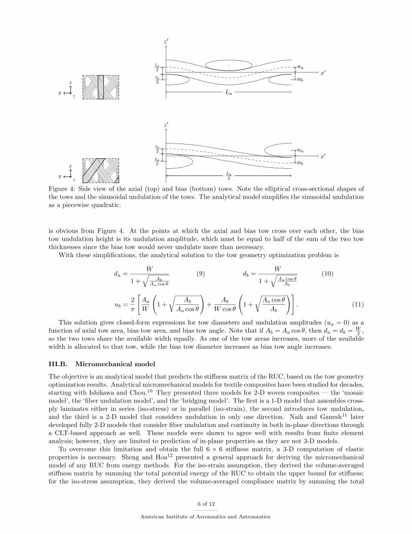
The representative unit cell is the smallest repeating unit in the 2DTBC architecture, shown in Figure3. An RUC contains two wavelengths of the axial tow aligned with the unit cell coordinate frame as well asone wavelength each of the +θ◦ and −θ◦ bias tows. The axial and bias tow undulations are shown in Figure4.

The RUC has a height H, length L, and width 2W , where W is the distance between two adjacent axialtows. The axial and bias tow areas, diameters, and thicknesses are represented by Aa, Ab, da, db, ta, and tb.The axial tow area and diameter in the plane of the bias tow undulation are Aa and da; likewise, the biastow area and diameter in the plane of the axial tow undulation are Ab and db. The relationships betweenthese RUC dimensions are

La =W

tan θ(1) da = da sin θ (2) Aa = Aa sin θ (3) Aa = π

da2

ta2

(4)

Lb =2W

sin θ(5) db = db sin θ (6) Ab = Ab sin θ (7) Ab = π

db2

tb2. (8)

The following description of the analytical model consists of two parts: the tow arrangement optimization,which predicts the geometry of the RUC, and the micromechanical model, which estimates the full 3-Dstiffness matrix using the modeled geometry.

III.A. Tow arrangement optimization

One of the requirements for design optimization with textile composites is a model for the tow geometry asa function of the design variables. For any combination of Aa, Ab, and θ, we want to be able to computeundulation amplitudes ua and ub as well as tow cross-sectional properties. The most accurate approach wouldbe to perform a simulation of the textile process used in manufacturing, considering the full geometries ofthe tows — including their tendency to twist and deform — while applying tensile loads to tighten the braidas is done in reality. Miao et al.8 implemented such an approach, using a digital element model to obtain aprecise prediction of the tow geometry and correctly capturing the twisting effect due to interaction betweentows. Here, we desire closed-form expressions describing the tow geometry — in other words, an analyticalsolution to the following optimization problem:

4 of 12

American Institute of Aeronautics and Astronautics

Figure 3: The 2DTBC architecture and its representative unit cell for small diameter tows (top) and largediameter tows (bottom).

maximize RUC fiber density

with respect to [da, db, ua, ub]T

subject to inequality constraints enforcing geometric compatibility

The optimization problem essentially solves a packing problem, reflecting actual manufacturing processeswhich attempt to maximize the fiber volume fraction. Since the fiber and matrix densities are typically onthe same order but the fiber is much stiffer, particularly in the axial direction, it is productive to increasethe fiber volume fraction as much as possible.

The above optimization problem can be quantified by assuming that the tows cross sections are alwayselliptical (the tows do not deform) and that their undulation path is periodic with no twist. Still, it is toocomplex to solve analytically because of the inequality constraints that ensure compatibility. This issue canbe resolved by making the following assumptions:

1. ua = 0

2. da + dbcos θ = W

3. ub = ta2 + tb

2

The first simplification is the assumption that the axial tows do not undulate. Typically, the axial towis aligned with the direction in which the axial stress is the largest, so the axial tow is also the largest inarea and stiffest. More importantly, the wavelength of the axial tow is less than half of that of the biastow, which makes the axial tow tend to be more flat because any undulation would yield a relatively largespatial frequency. This assumption has been made in other models in the literature with good results.9

Qualitatively, the second simplification is simply a statement that, during the textile process, the axial andbias tows will widen until they are in contact with each other. Since the number of fibers in a tow isfixed, the tow areas are also roughly constant, so the tendency of the tows to flatten in order to decreasetheir undulation amplitudes results in a corresponding increase in tow diameters. The final simplification

5 of 12

American Institute of Aeronautics and Astronautics

x

yz

z′

x′ta2

tb2

ua

ub

La

x

yz

z′

x′ta2

tb2 ua

ub

Lb

2

Figure 4: Side view of the axial (top) and bias (bottom) tows. Note the elliptical cross-sectional shapes ofthe tows and the sinusoidal undulation of the tows. The analytical model simplifies the sinusoidal undulationas a piecewise quadratic.

is obvious from Figure 4. At the points at which the axial and bias tow cross over each other, the biastow undulation height is its undulation amplitude, which must be equal to half of the sum of the two towthicknesses since the bias tow would never undulate more than necessary.

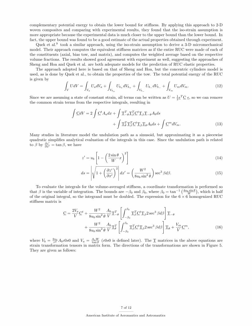
With these simplifications, the analytical solution to the tow geometry optimization problem is

da =W

1 +√

Ab

Aa cos θ

(9) db =W

1 +√

Aa cos θAb

(10)

ub =2

π

[AaW

(1 +

√Ab

Aa cos θ

)+

AbW cos θ

(1 +

√Aa cos θ

Ab

)]. (11)

This solution gives closed-form expressions for tow diameters and undulation amplitudes (ua = 0) as afunction of axial tow area, bias tow area, and bias tow angle. Note that if Ab = Aa cos θ, then da = db = W

2 ,so the two tows share the available width equally. As one of the tow areas increases, more of the availablewidth is allocated to that tow, while the bias tow diameter increases as bias tow angle increases.

III.B. Micromechanical model

The objective is an analytical model that predicts the stiffness matrix of the RUC, based on the tow geometryoptimization results. Analytical micromechanical models for textile composites have been studied for decades,starting with Ishikawa and Chou.10 They presented three models for 2-D woven composites — the ‘mosaicmodel’, the ‘fiber undulation model’, and the ‘bridging model’. The first is a 1-D model that assembles cross-ply laminates either in series (iso-stress) or in parallel (iso-strain), the second introduces tow undulation,and the third is a 2-D model that considers undulation in only one direction. Naik and Ganesh11 laterdeveloped fully 2-D models that consider fiber undulation and continuity in both in-plane directions througha CLT-based approach as well. These models were shown to agree well with results from finite elementanalysis; however, they are limited to prediction of in-plane properties as they are not 3-D models.

To overcome this limitation and obtain the full 6 × 6 stiffness matrix, a 3-D computation of elasticproperties is necessary. Sheng and Hoa12 presented a general approach for deriving the micromechanicalmodel of any RUC from energy methods. For the iso-strain assumption, they derived the volume-averagedstiffness matrix by summing the total potential energy of the RUC to obtain the upper bound for stiffness;for the iso-stress assumption, they derived the volume-averaged compliance matrix by summing the total

6 of 12

American Institute of Aeronautics and Astronautics

complementary potential energy to obtain the lower bound for stiffness. By applying this approach to 2-Dwoven composites and comparing with experimental results, they found that the iso-strain assumption ismore appropriate because the experimental data is much closer to the upper bound than the lower bound. Infact, the upper bound was found to be a good estimate of the actual properties obtained through experiment.

Quek et al.9 took a similar approach, using the iso-strain assumption to derive a 3-D micromechanicalmodel. Their approach computes the equivalent stiffness matrices as if the entire RUC were made of each ofthe constituents (axial, bias tow, and matrix), and computes the weighted average based on the respectivevolume fractions. The results showed good agreement with experiment as well, suggesting the approaches ofSheng and Hoa and Quek et al. are both adequate models for the prediction of RUC elastic properties.

The approach adopted here is based on that of Sheng and Hoa, but the concentric cylinders model isused, as is done by Quek et al., to obtain the properties of the tow. The total potential energy of the RUCis given by ∫

V

UdV =

∫Va

UadVa +

∫Vb+

Ub+dVb+ +

∫Vb−

Ub−dVb− +

∫Vm

UmdVm. (12)

Since we are assuming a state of constant strain, all terms can be written as U = 12εTC ε, so we can remove

the common strain terms from the respective integrals, resulting in∫CdV = 2

∫CtAadx+

∫TT−θT

TβCtTβT−θAbds

+

∫TTθ TTβCtTβTθAbds+

∫CmdVm. (13)

Many studies in literature model the undulation path as a sinusoid, but approximating it as a piecewisequadratic simplifies analytical evaluation of the integrals in this case. Since the undulation path is relatedto β by ∂z′

∂x′ = tanβ, we have

z′ = ub

[1−

(2 sin θ

Wx

)2]

(14)

ds =

∣∣∣∣∣∣√

1 +

(∂z′

∂x′

)2∣∣∣∣∣∣ dx′ =

(W 2

8ub sin2 θ

)sec3 βdβ. (15)

To evaluate the integrals for the volume-averaged stiffness, a coordinate transformation is performed sothat β is the variable of integration. The bounds are −β0 and β0, where β0 = tan−1

(4ub sin θW

), which is half

of the original integral, so the integrand must be doubled. The expression for the 6 × 6 homogenized RUCstiffness matrix is

C =2VaV

Ct +W 2

8ub sin2 θ

AbV

TT−θ

[∫ β0

−β0

TTβCtTβ2 sec3 βdβ

]T−θ

+W 2

8ub sin2 θ

AbV

TTθ

[∫ β0

−β0

TTβCtTβ2 sec3 βdβ

]Tθ +

VmV

Cm, (16)

where Vb = 2ub

r2 Abc0s0 and Va = AaWtan θ (c0s0 is defined later). The T matrices in the above equations are

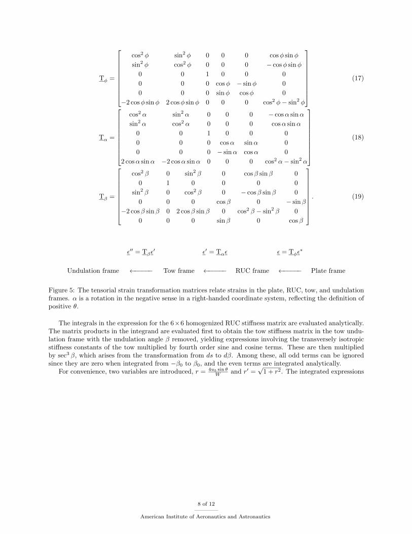
strain transformation tensors in matrix form. The directions of the transformations are shown in Figure 5.They are given as follows:

7 of 12

American Institute of Aeronautics and Astronautics

Tφ =

cos2 φ sin2 φ 0 0 0 cosφ sinφ

sin2 φ cos2 φ 0 0 0 − cosφ sinφ

0 0 1 0 0 0

0 0 0 cosφ − sinφ 0

0 0 0 sinφ cosφ 0

−2 cosφ sinφ 2 cosφ sinφ 0 0 0 cos2 φ− sin2 φ

(17)

Tα =

cos2 α sin2 α 0 0 0 − cosα sinα

sin2 α cos2 α 0 0 0 cosα sinα

0 0 1 0 0 0

0 0 0 cosα sinα 0

0 0 0 − sinα cosα 0

2 cosα sinα −2 cosα sinα 0 0 0 cos2 α− sin2 α

(18)

Tβ =

cos2 β 0 sin2 β 0 cosβ sinβ 0

0 1 0 0 0 0

sin2 β 0 cos2 β 0 − cosβ sinβ 0

0 0 0 cosβ 0 − sinβ

−2 cosβ sinβ 0 2 cosβ sinβ 0 cos2 β − sin2 β 0

0 0 0 sinβ 0 cosβ

. (19)

ε′′ = Tβε′ ε′ = Tαε ε = Tφε

∗

Undulation frame ←−−−−− Tow frame ←−−−−− RUC frame ←−−−−− Plate frame

Figure 5: The tensorial strain transformation matrices relate strains in the plate, RUC, tow, and undulationframes. α is a rotation in the negative sense in a right-handed coordinate system, reflecting the definition ofpositive θ.

The integrals in the expression for the 6×6 homogenized RUC stiffness matrix are evaluated analytically.The matrix products in the integrand are evaluated first to obtain the tow stiffness matrix in the tow undu-lation frame with the undulation angle β removed, yielding expressions involving the transversely isotropicstiffness constants of the tow multiplied by fourth order sine and cosine terms. These are then multipliedby sec3 β, which arises from the transformation from ds to dβ. Among these, all odd terms can be ignoredsince they are zero when integrated from −β0 to β0, and the even terms are integrated analytically.

For convenience, two variables are introduced, r = 4ub sin θW and r′ =

√1 + r2. The integrated expressions

8 of 12

American Institute of Aeronautics and Astronautics

for each trigonometric term are

c4 =4r

r′(20)

c2s2 =−4r

r′+ 2 ln

(1 + r

r′

1− rr′

)(21)

s4 =4r

r′+

1

1− rr′− 1

1 + rr′− 7

4ln(

1 +r

r′

)+

3

2ln(

1− r

r′

)(22)

c2 = 2 ln

(1 + r

r′

1− rr′

)(23)

s2 = 2rr′ − ln

(1 + r

r′

1− rr′

)(24)

c0s0 = 2rr′ + ln

(1 + r

r′

1− rr′

), (25)

where c4 = 2∫ β0

−β0cos4 β sec3 βdβ, as an example. Then, the integrated stiffness matrix in the F ′ frame is

2

∫ β0

−β0

TTβCtTβ sec3 βdβ =

C ′11 C ′12 C ′13 0 0 0

C ′12 C ′22 C ′23 0 0 0

C ′13 C ′23 C ′33 0 0 0

0 0 0 C ′44 0 0

0 0 0 0 C ′55 0

0 0 0 0 0 C ′66

(26)

C ′11 = Ct11c4 + (2Ct12 + 4Ct55)c2s2 + Ct22s4 (27)

C ′12 = Ct12c2 + Ct23s2 (28)

C ′13 = Ct12c4 + (Ct11 + Ct22 − 4Ct55)c2s2 + Ct12s4 (29)

C ′22 = Ct22c0s0 (30)

C ′23 = Ct23c2 + Ct12s2 (31)

C ′33 = Ct22c4 + (2Ct12 + 4Ct55)c2s2 + Ct11s4 (32)

C ′44 = Ct44c2 + Ct66s2 (33)

C ′55 = Ct55c4 + (Ct11 − 2Ct12 + Ct22 − 2Ct55)c2s2 + Ct55s4 (34)

C ′66 = Ct66c2 + Ct44s2. (35)

IV. Application

IV.A. Validation

Table 1 compares the results obtained from the current model with those obtained experimentally andanalytically by Kier et al.13 In general, the current model does not agree as well as the Quek model withone notable exception. The experimentally measured Gxy constant increases with increasing bias tow angle,which is captured by the current model, but the opposite is true with the Quek model. It is hypothesizedthat this difference is caused by the fact that the current model correctly predicts that with increasing biastow angle, the bias tow undulation increases, increasing the RUC volume and increasing the relative amountof matrix in the RUC. Since the matrix material makes a larger contribution to in-plane shear stiffness, thistrend offsets the influence of the bias tow contribution, which changes as the bias tow angle varies.

Overall, the current model is not as accurate as existing models, but the key difference is that the currentmodel computes the tow geometry automatically, with only tow areas, bias tow angle, and fiber volumefraction required as input variables. Existing models require many more variables to be experimentallymeasured to be able to compute the stiffness matrix. With the current model, the trends were predictedsatisfactorily, and optimization is possible with this new model.

9 of 12

American Institute of Aeronautics and Astronautics

30◦ Experimental Quek Current

Ex[GPa] 53.1± 0.8 58.3 50.5

Ey[GPa] 7.3± 0.5 8.06 9.19

Gxy[GPa] 8.3± 2.5 10.8 9.45

νxy 0.93 0.995 0.76

Gyx[GPa] 15.4± 3.2

45◦ Experimental Quek Current

Ex[GPa] 27.9± 1.1 29.4 30.3

Ey[GPa] 13.7± 1.2 13.9 17.6

Gxy[GPa] 10.8± 2.0 9.35 9.79

νxy 0.59 0.535 0.49

Gyx[GPa] 14.4± 4.0

60◦ Experimental Quek Current

Ex[GPa] 23.2± 0.8 28.4 27.0

Ey[GPa] 22.1± 0.1 22.6 26.9

Gxy[GPa] 11.8± 2.7 8.85 10.9

νxy 0.30 0.328 0.31

Gyx[GPa] 11.9± 1.3

Table 1: Comparison between the results from the current analytical model and the analytical results fromQuek’s model and experimental results presented in Kier et al.13

IV.B. Optimization Problem

For a single-layer homogeneous laminate, bending and stretching are not coupled and the vector of loads Nand M can be combined to form a single vector that induces a maximum in-plane strain of ε:{

N

M

}=

[A 0

0 D

]{ε0

κ

}(36)

ε0 = A−1N =1

hC−1N (37)

κ = D−1M =12

h3C−1M (38)

ε = ε0 + zκ =1

hC−1

(N + z

12

h2M

). (39)

The general optimization problem is

minimize RUC areal density

with respect to [θ, h, φ,Aa, Ab]T

subject to tow strains less than 0.005

matrix shear stress less than 5 MPa

The tow strains are very insensitive to the magnitudes of Aa and Ab, so the plate thickness, h, is animportant variable for scaling the problem based on the magnitudes of the loads applied. The remainingdegrees of freedom — θ, φ, and Aa/Ab — all have a similar effect of redistributing stiffness among the variouscomponents as opposed to changing its effective magnitude.

To simplify the problem, it is assumed here that only in-plane stresses are applied. φ can be chosen toalign the RUC with the principal directions such that the axial tow is parallel to the largest principal stress.This yields a new Nx and Ny in the RUC frame with no shear stress component. If we denote N∗x , N∗y , and

10 of 12

American Institute of Aeronautics and Astronautics

N∗xy the stresses in the original plate frame, we have φ = 12 tan−1

2N∗xy

N∗x−N∗y and the tow strains can be found

using {εa

εb

}=

[1 0

cos2 θ sin2 θ

]{εx

εy

}(40)

{εa

εb

}=

1

h

[1 0

cos2 θ sin2 θ

][C11 C12

C12 C22

]−1{Nx

Ny

}(41)

{εa

εb

}=

1

h

[1 0

cos2 θ sin2 θ

][C11 C12

C12 C22

]−1 [cos2 φ sin2 φ 2 cosφ sinφ

sin2 φ cos2 φ −2 cosφ sinφ

]N∗xN∗yN∗xy

. (42)

The elastic constants are insensitive to proportional increases to Aa and Ab; however, they are moresensitive to the ratio between the tow areas. From the tow geometry optimization, Aa must be sufficientlygreater than Ab for the assumption to be valid that the axial tow does not undulate. However, the biastow area should not be too small as it serves a dual purpose of carrying the loads in the y direction andproviding more balanced stiffness even when Ny is small for considerations such as impact resistance. Forthe numerical optimization results that follow, a ratio of 4 is used as a compromise.

IV.C. Numerical Optimization

From the previous discussion, the remaining design variables are θ and h. φ is used to align the RUC withthe principal directions, and the tow areas are chosen to give a ratio of 4. Realistic values for the tow areasare Aa/W

2 = 0.08 and Ab/W2 = 0.02. The numerical optimization problem for a given plate with a given

loading is then as follows:

minimize RUC areal density

with respect to [θ, h/W ]T

subject to |εa| ≤ 0.005

|εb| ≤ 0.005

Since the optimization problem is continuous, it is solved using SNOPT, a Sequential Quadratic Pro-gramming (SQP) algorithm that handles nonlinear, convex optimization problems very well.14 SQP methodsdefine a quadratic sub-problem with linearized constraints at every major iteration, approximating the Hes-sian matrix with the widely-used BFGS update formula and using a line search along each computed searchdirection. Here, gradients computed using the finite difference method provide sufficient accuracy — opti-mality and feasibility are converged to 10−10.

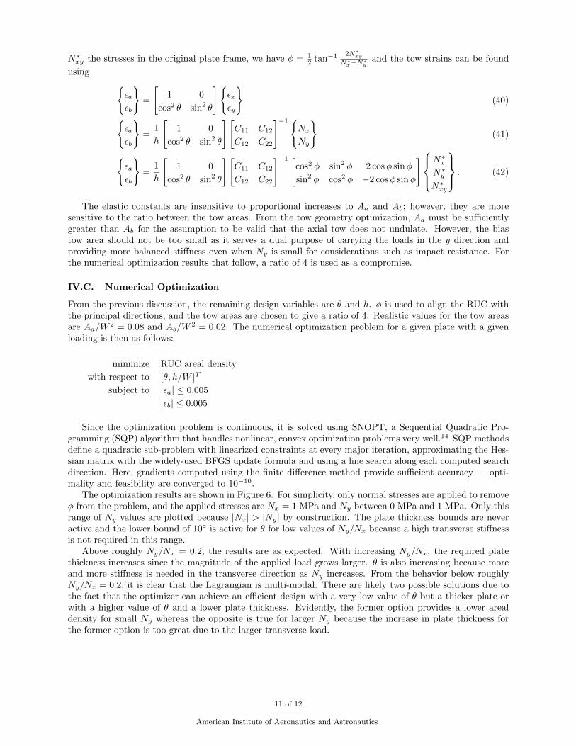
The optimization results are shown in Figure 6. For simplicity, only normal stresses are applied to removeφ from the problem, and the applied stresses are Nx = 1 MPa and Ny between 0 MPa and 1 MPa. Only thisrange of Ny values are plotted because |Nx| > |Ny| by construction. The plate thickness bounds are neveractive and the lower bound of 10◦ is active for θ for low values of Ny/Nx because a high transverse stiffnessis not required in this range.

Above roughly Ny/Nx = 0.2, the results are as expected. With increasing Ny/Nx, the required platethickness increases since the magnitude of the applied load grows larger. θ is also increasing because moreand more stiffness is needed in the transverse direction as Ny increases. From the behavior below roughlyNy/Nx = 0.2, it is clear that the Lagrangian is multi-modal. There are likely two possible solutions due tothe fact that the optimizer can achieve an efficient design with a very low value of θ but a thicker plate orwith a higher value of θ and a lower plate thickness. Evidently, the former option provides a lower arealdensity for small Ny whereas the opposite is true for larger Ny because the increase in plate thickness forthe former option is too great due to the larger transverse load.

11 of 12

American Institute of Aeronautics and Astronautics

0.0 0.2 0.4 0.6 0.8 1.0Ny/Nx

10

20

30

40

50

60

70

80

Thet

a [d

egre

es]

0.0 0.2 0.4 0.6 0.8 1.0Ny/Nx

3.0

3.5

4.0

4.5

5.0

5.5

Plat

e th

ickn

ess

[mm

]

Figure 6: Optimized values of θ and h plotted versus Ny/Nx. The axial load applied is Nx = 1 MPa.

V. Conclusion

The model developed in this paper addresses some of challenges associated with performing aeroelas-tic tailoring with 2-D triaxial braided composites. The RUC geometry is modeled using an optimizationformulation for the packing problem which provides a closed form solution that is used as part of the mi-cromechanical model. Existing models require experimental measurement of numerous geometric propertiesfor a given RUC configuration, which prohibits design optimization because these inevitably vary as the de-sign variables change. The micromechanical uses a volume-averaged stiffness approach under the iso-strainassumption, and closed-form solutions are obtained here as well. The computed elastic constants show goodagreement with experiment in most cases, and when they do not, the error is likely due to the tow geome-try model. Preliminary results from numerical design optimization of the RUC are robust and agree withintuition.

References

1Shirk, M. H., Hertz, T. J., and Weisshaar, T., “Aeroelastic tailoring — theory, practice, and promise,” Journal of Aircraft ,Vol. 23, No. 1, 1986, pp. 6–18.

2Librescu, L. and Song, O., “On the static aeroelastic tailoring of composite aircraft swept wings modelled as thin-walledbeam structures,” Composites Engineering, Vol. 2, No. 5-7, 1992, pp. 497–512.

3Eastep, F. E., Tischler, V. A., Venkayya, V. B., and Khot, N. S., “Aeroelastic Tailoring of Composite Structures,” Journalof Aircraft , Vol. 36, No. 6, 1999, pp. 1041–1047.

4Weisshaar, T. and Duke, D., “Induced Drag Reduction Using Aeroelastic Tailoring with Adaptive Control Surfaces,”Journal of Aircraft , Vol. 43, No. 1, 2006, pp. 157–164.

5Guo, S., Cheng, W., and Cui, D., “Aeroelastic Tailoring of Composite Wing Structures by Laminate Layup Optimization,”AIAA Journal , 2006, pp. 3146–3150.

6Kennedy, G. J. and Martins, J. R. R. A., “Aerostructural design optimization of composite aircraft with stress and localbuckling constraints using an implicit structural parametrization,” April 2011.

7Tong, L., Mouritz, A. P., and Bannister, M. K., 3D Fibre Reinforced Polymer Composites, Elsevier, 2002.8Miao, Y., Zhou, E., Wang, Y., and Cheeseman, B. A., “Mechanics of textile composites: Micro-geometry,” Composites

Science and Technology, Vol. 68, No. 7-8, 2008, pp. 1671–1678.9Quek, S. C., Waas, A. M., Shahwan, K. W., and Agaram, V., “Analysis of 2D triaxial flat braided textile composites,”

International Journal of Mechanical Sciences, Vol. 45, No. 6-7, 2003, pp. 1077–1096.10Ishikawa, T. and Chou, T. W., “Stiffness and strength behaviour of woven fabric composites,” Journal of Materials

Science, Vol. 17, No. 11, 1982, pp. 3211–3220.11Naik, N. K. and Ganesh, V. K., “Prediction of on-axes elastic properties of plain weave fabric composites Naik, N.K.

and Ganesh, V.K. Composites Science and Technology Vol 44 No 22 (1992) pp 135152,” Composites, Vol. 24, No. 4, 1993,pp. 368–368.

12Sheng, S. Z. and Hoa, S. V., “Three Dimensional Micro-MechanicalModeling of Woven Fabric Composites,” Journal ofComposite Materials, Vol. 35, No. 19, 2001, pp. 1701–1729.

13Kier, Z. T., Salvi, A., Theis, G., Waas, A. M., and Shahwan, K., “Predicting Mechanical Properties of 2D TriaxiallyBraided Textile Composites Based on Microstructure Properties,” 2010.

14Gill, P., Murray, W., and Saunders, M., “SNOPT: An SQP algorithm for large–scale constraint optimization,” SIAMJournal of Optimization, Vol. 12, No. 4, 2002, pp. 979–1006.

12 of 12

American Institute of Aeronautics and Astronautics