Nasa Contractor Report 204153

Micromechanical Modeling of Woven Metal Matrix Composites

Brett A. Bednarcyk and Marek-Jerzy Pindera University of Virginia, Charlottesville, Virginia

National Aeronautics and Space Administration

Prepared under Grant NAG3-1316 Lewis Research Center

October 1997

https://ntrs.nasa.gov/search.jsp?R=19970041400 2019-08-14T03:42:45+00:00Z

Acknowlegments

This investigation was funded by NASA Lewis Research Center under Grant NAG3-1319 with Dr. Robert V. Miner as the technical monitor. The authors gratefully acknowledge this support and the

assistance of Dr. David L. Ellis, Dr. Robert V. Miner, and Dr. Michael V. Nathal of NASA Lewis Research Center and Dr. Sandra M. DeVincent of Metal Matrix Castings, Inc.

This report is a presentation of preliminary findings, subject to revision

as analysis proceeds.

Trade names or manufacturers' names are used in this report for identification only. This usage does not constitute an official endorsement, either expressed or implied, by the National

Aeronautics and Space Administration.

NASA Center for Aerospace Information 800 Elkridge Landing Road Lynthicum, MD 21090-2934 Price Code: A07

Available from

National Technical Information Service 5287 Port Royal Road Springfield, VA 22100

Price Code: A07

Abstract

This report presents the results of an extensive micromechanical modeling effort for woven metal matrix composites. The model is employed to predict the mechanical response of 8-harness (8H) satin carbodcopper (C/Cu) composites. Experimental mechanical results for this novel high thermal conductivity material were recently reported by Bednarcyk et al. (1997) along with preliminary model results.

The micromechanics model developed herein is based on an embedded approach. A micromechanics model for the local (micro-scale) behavior of the woven composite, the original method of cells (Aboudi, 1987), is embedded in a global (macro-scale) micromechanics model (the three-dimensional generalized method of cells (GMC-3D) (Aboudi, 1994)). This approach allows representation of true repeating unit cells for woven metal matrix composites via GMC- 3D, and representation of local effects, such as matrix plasticity, yam porosity, and imperfect fiber-matrix bonding. In addition, the equations of GMC-3D were reformulated to significantly reduce the number of unknown quantities that characterize the deformation fields at the micro- level in order to make possible the analysis of actual microstructures of woven composites. The resulting micromechanical model (WCGMC) provides an intermediate level of geometric representation, versatility, and computational efficiency with respect to previous analytical and numerical models for woven composites, but surpasses all previous modeling work by allowing the mechanical response of a woven metal matrix composite, with an elastoplastic matrix, to be examined for the first time.

WCGMC is employed to examine the effects of composite microstructure, porosity, residual stresses; and imperfect fiber-matrix bonding on the predicted mechanical response of 8H satin CfCu. The previously reported experimental results are summarized, and the model predictions are compared to monotonic and cyclic tensile and shear test data. By considering appropriate levels of porosity, residual stresses, and imperfect fiber-matrix debonding, reasonably good qualitative and quantitative correlation is achieved between model and experiment.

Table of Contents

. . Abstract .............................................................................................................................. 11

... ................................................................................................................. Acknowledgments 111

.................................................................................................................. Table of Contents iv

1 . Introduction ................................................................................................................... 1 1.1 Woven Composites ................................................................................................ 1 1.2 Modeling of Woven Composites .............................................................................. 3

............................................... 1.2.1 Finite-Element and Boundary-Element Models 3 ....................................................................... 1.2.2 Approximate Analytical Models 5

1.3 Objectives of Present Investigation .......................................................................... 8

2 . Analytical Model . WCGMC ........................................................................................... 11 .............................................................................. 2.1 GMC-3D . Original Formulation 12

2.2 GMC-3D . Reformulation ........................................................................................ 16 2.3 Heterogeneous Subcells via the Reformulated Original Method of Cells

with Imperfect Fiber Matrix Bonding ....................................................................... 24 ................................................................................................. 2.4 Brayshaw Averaging 37

2.5 Classical Incremental Plasticity Theory .................................................................... 43 ...................................................... 2.6 Solution Procedure in the Presence of Plasticity 45

3 . Modeling the Mechanical Response of 8-Harness Satin CICu ........................................ 48 ................................ 3.1 Effect of Unit Cell Microstructure and Fiber Volume Fraction 48

3.1.1 Tensile Response .............................................................................................. 53 ................................................................................................. 3.1.2 Shear Response 58

..................................................... 3.1.3 Summary of Fiber Volume Fraction Effects 61 3.2 Effect of Porosity ...................................................................................................... 63

........................................................................................ 3.3 Effect of Residual Stresses 66 3.4 Effect of Imperfect Fiber-Matrix Bonding ................................................................ 76

................................................................................................... 3.4.1 Elastic Moduli 76 ........................................................................................ 3.4.2 Mechanical Response 80

3.5 Summary of Modeled Effects ................................................................................... 83

........................................................................................ 4 . Model-Experiment Correlation 85 4.1 Summary of Experimental Results ........................................................................... 85

................................................................................................. 4.2 Monotonic Response 91 ........................................................................................................ 4.3 Cyclic Response 99

.............................................................................................. 5 . Summary and Conclusions 105

References .... . . . . . . . . . . . . . . . . . . . . . . . . . . . . . . . . . . . . . . . . . . . . . . . . . . . . . . . . . . . . . . . . . . . . . , . . . . . . . . . . . . . . . . . . . . . . . . . . . . . . . . . . . . . . . . . . . . . . . . . . . 109

Appendix . . ... . . . . . . . . . . . . . . . . . . . . . . . . . . . . . . . . . . . . . . . . . . . . . . . . . . . . . . . . . . . . . . . . . . . . . . . . . . . . . . . . . . . . . . . . . . . . . . . . . . . . . . . . . . . . . . . . . . . . . . . . . . 1 12

1. Introduction

1.1 Woven Composites

Research on the manufacturing, testing, and modeling of woven and braided composites

has increased significantly in recent years. The reinforcement phase of these composites consists

of a woven or braided fabric formed by individual fibers, or by bundles of fibers, called yams.

One or more layers of the woven or braided fabric are used to reinforce traditional matrix

materials. It is interesting to note that the concept of woven composites is not a new one.

Ancient Egyptians used cotton fabrics impregnated with resin to protect fkagile mummies. The

effort to use woven composites for thermal and structural applications, though possibly less

captivating, is considerably more recent.

By incorporating a woven reinforcement phase into a composite, rather than utilizing

unidirectional fibers only, several benefits are realized. A single ply of a woven composite can

have equivalent thermomechanical properties in several directions. A single ply reinforced by a

biaxial weave is geometrically similar to a [0°/900] laminate, while a ply reinforced by a triaxial

weave can mimic a [0°/k600] laminate, as illustrated in Figure 1.1. In contrast, a unidirectional

ply often has poor thermomechanical properties transverse to the fiber direction due to the lack of

continuous reinforcement in this direction. The deficiency of a continuous ply in the transverse

direction is often exacerbated by a weak fiberlmatrix interface.

BIAXIAL WEAVE TRlAXlAL WEAVE

Figure 1.1. a) Biaxial weave pattem; b) Triaxial weave pattem (Chou, et al., 1986).

Woven and braided composites usually have superior out-of-plane properties with regard

to impact and crack resistance relative to composites laminated with unidirectional plies. In fact,

coated fabrics, which are in essence woven composites, are used to make bullet proof vests.

Movement of the reinforcement weave can distribute the energy of an impact throughout many

yarns, and, if a crack does form, there are fibers oriented in at least two distinct directions to

inhibit crack growth. Since the reinforcement phase has a tendency to remain intact

independently from the matrix, woven composites are less prone to delamination and splitting

along the fibers. The work of Kaliakin et al. (1996) indicates that these properties give woven

composites the potential to serve a major role in concrete structure strengthening through the

application of woven composite plates or jackets directly to the concrete surface.

Finally, and perhaps most importantly, a woven or braided reinforcement phase offers

superior stability during composite manufacturing compared to unidirectional fibers. A weave of

fiber yams is much simpler to handle than the thousands of individual fibers used in a graphite

fiber reinforced composite, for example. The benefits of the weave's dimensional stability go

further. Preforms with complex shapes can be woven or braided from the fiber yarns. These

shapes can then be infiltrated with a metal or epoxy matrix to form a composite in the shape of

the preform. This procedure is not feasible if individual unidirectional fibers are used. In

addition, three-dimensional weaves and braids can be produced (see Figure 1.2). A third

dimension of reinforcement can improve the properties of the composite even M e r .

THREE.DIMENSIONAL CYLINDRICAL CONSTRUCTION THREE-DIMENSIONAL BRAIDING

Figure 1.2. Examples of 3-D weave patterns. a) Cylindrical construction. b) 3-D braiding (Chou, et al., 1986).

1.2 Modeling of Woven Composites

While woven composites offer advantages over unidirectional composites and laminates,

they are also more challenging to model. The woven reinforcement phase consists of yarns that

undulate in and out of a plane. Thus the geometry of the composite is inherently three-

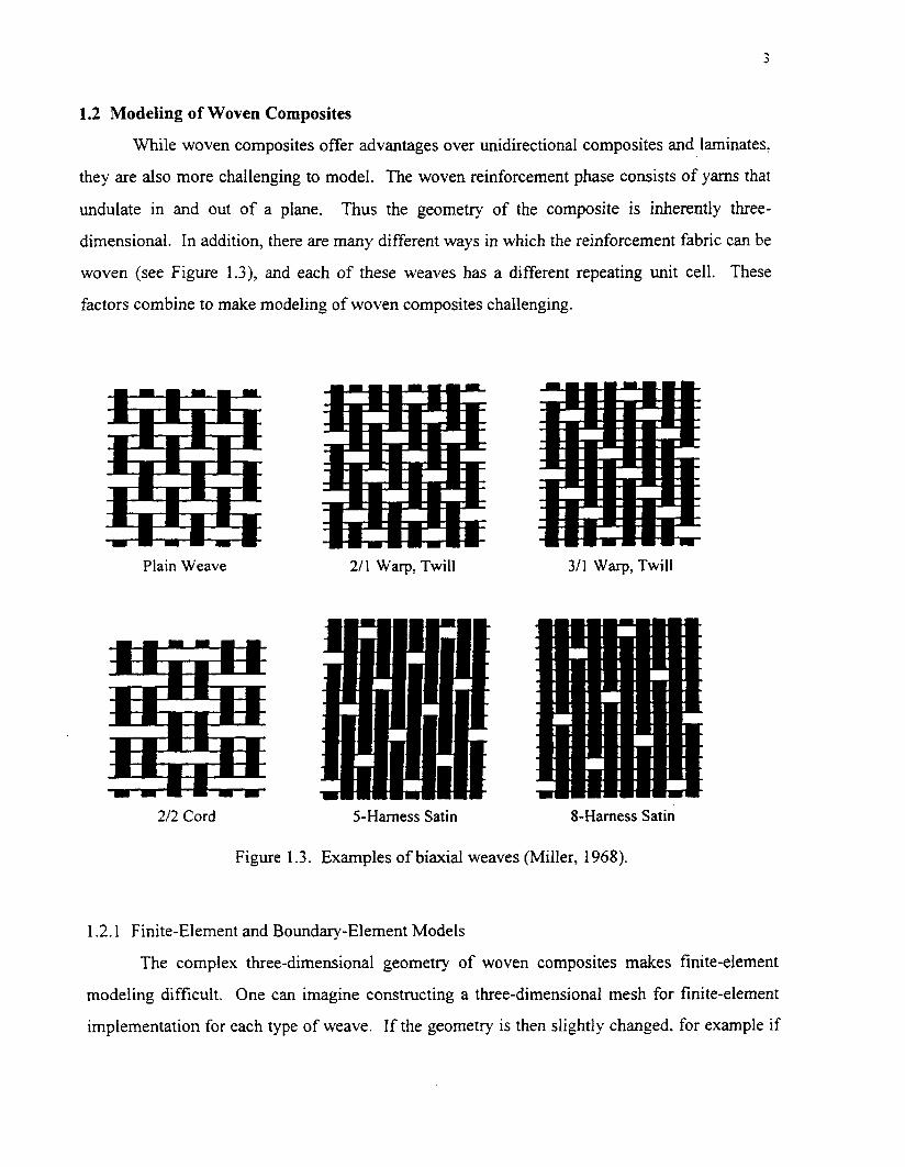
dimensional. In addition, there are many different ways in which the reinforcement fabric can be

woven (see Figure 1.3), and each of these weaves has a different repeating unit cell. These

factors combine to make modeling of woven composites challenging.

Plain Weave 211 Warp, Twill 311 Warp, Twill

2/2 Cord 5-Harness Satin %Harness Satin

Figure I .3. Examples of biaxial weaves (Miller, 1968).

1.2.1 Finite-Element and Boundary-Element Models

The complex three-dimensional geometry of woven composites makes finite-element

modeling difficult. One can imagine constructing a three-dimensional mesh for finite-element

implementation for each type of weave. If the geometry is then slightly changed. for example if

adjacent yarns are placed closer together, an entirely new mesh would be necessary. The effort

required for such numerical modeling may be prohibitive. However, this type of effort was

undertaken by Dasgupta and Bhandarkar (1994) and Dasgupta et al. (1996) to model the elastic

behavior of a plain weave glasslepoxy composite. In this investigation, reasonable elastic

constants were predicted for a realistic geometric representation of the composite, but only with

great computational effort.

Whitcomb et al. (1992) proposed a finite-element model for woven composites in which

spatial variations of material properties were accounted for within a single element. This

approach could potentially decrease the number of elements required to accurately model the

geometry of a woven composite. However, a traditional three-dimensional finite-element

analysis was used by Whitcomb and Srirengan (1996) to model progressive failure in plain

weave graphitelepoxy composites with varying degrees of fiber waviness. The finite-element

approach was also used by Glaessgen et al. (1996) to examine the internal displacement and

strain energy density fields in a plain weave glasslepoxy composite. Here, geometric

complexities inherent to woven reinforcements (which greatly affect internal fields) are

accounted for, but at a high computational cost.

Marrey and Sankar (1997) performed elastic finite element analyses of plain weave and

5-harness satin composite plates through the use of homogenized brick elements. Effective

properties of the brick elements, which represent the composite repeating unit cell, were first

determined via finite element analysis. Then these homogenized elements were assembled,

under appropriate boundary conditions to form a plate. It should be noted that the above finite-

element analyses considered only woven composites with elastic phases. Due to the complex

geometry of woven composites (and thus the large number of degrees of freedom), inclusion of

matrix inelasticity in finite element models for these materials would require immense execution

times. Analysis of a simple woven metal matrix composite (with an elastoplastic matrix) via

finite elements may be possible through the use of supercomputers, but to date, such an analysis

has not been reported.

A boundary-element model developed by Goldberg and Hopkins (1995) that has been

used to examine the elastic response of woven composites deserves reference. The boundary-

element method requires less computational and mesh generating effort than the finite-element

method, yet it can offer similar geometrical accuracy for woven composites. A version of this

model with matrix inelasticity is under development and may have potential for modeling woven

metal matrix composites (Goldberg, 1996).

1 2.2 Approximate Analytical Models

Another route to modeling woven composites was taken by Chou and Ishikawa (1989).

These authors have developed a well-known series of models based on classical lamination

theory for predicting the thermoelastic response of certain types of woven composites. The

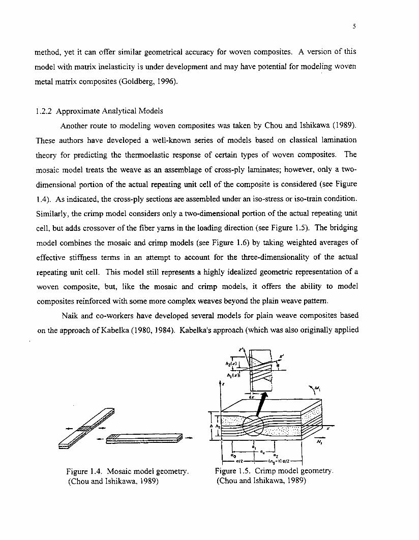
mosaic model treats the weave as an assemblage of cross-ply laminates; however, only a two-

dimensional portion of the actual repeating unit cell of the composite is considered (see Figure

1.4). As indicated, the cross-ply sections are assembled under an iso-stress or iso-train condition.

Similarly, the crimp model considers only a two-dimensional portion of the actual repeating unit

cell, but adds crossover of the fiber yarns in the loading direction (see Figure 1.5). The bridging

model combines the mosaic and crimp models (see Figure 1.6) by taking weighted averages of

effective stiffness terms in an attempt to account for the three-dimensionality of the actual

repeating unit cell. This model still represents a highly idealized geometric representation of a

woven composite, but, like the mosaic and crimp models, it offers the ability to model

composites reinforced with some more complex weaves beyond the plain weave pattern.

Naik and co-workers have developed several models for plain weave composites based

on the approach of Kabelka (1 980, 1984). Kabelka's approach (which was also originally applied

Figure 1.4. Mosaic model geometry. (Chou and Ishikawa, 1989)

Figure 1.5. Crimp model geometry. (Chou and Ishikawa, 1989)

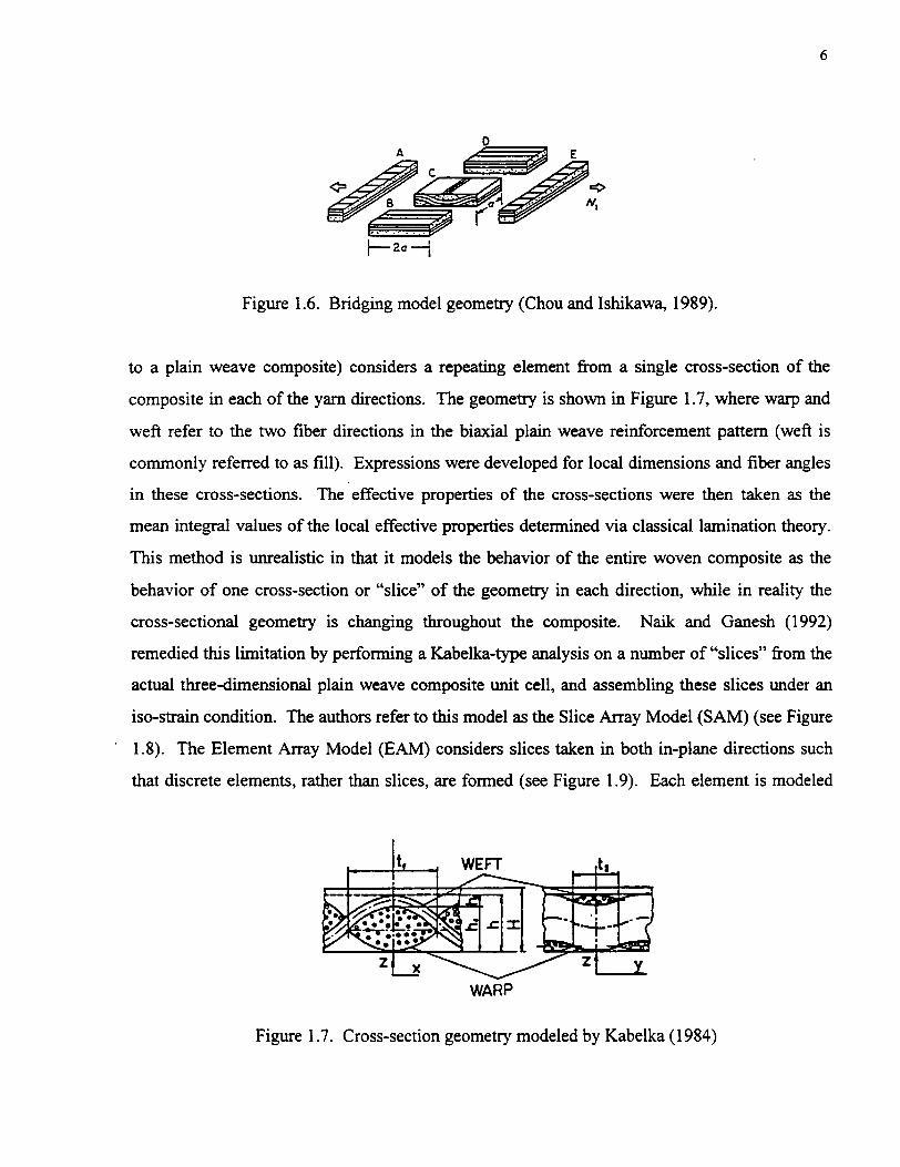
Figure 1.6. Bridging model geometry (Chou and Ishikawa, 1989).

to a plain weave composite) considers a repeating element from a single cross-section of the

composite in each of the yarn directions. The geometry is shown in Figure 1.7, where warp and

weft refer to the two fiber directions in the biaxial plain weave reinforcement pattern (weft is

commonly referred to as fill). Expressions were developed for local dimensions and fiber angles

in these cross-sections. The effective properties of the cross-sections were then taken as the

mean integral values of the local effective properties determined via classical lamination theory.

This method is unrealistic in that it models the behavior of the entire woven composite as the

behavior of one cross-section or "slice" of the geometry in each direction, while in reality the

cross-sectional geometry is changing throughout the composite. Naik and Ganesh (1992)

remedied this limitation by performing a Kabelka-type analysis on a number of "slices" fiom the

actual three-dimensional plain weave composite unit cell, and assembling these slices under an

iso-strain condition. The authors refer to this model as the Slice Array Model (SAM) (see Figure ' 1.8). The Element Array Model (EAM) considers slices taken in both in-plane directions such

that discrete elements, rather than slices, are formed (see Figure 1.9). Each element is modeled

WARP

Figure 1.7. Cross-section geometry modeled by Kabelka (1 984)

UNll CELL

Y

"1

ACTUAL SLICES IOEALlSEO SLKES

Figure 1.8. SAM model geometry (Naik and Ganesh, 1992).

SERIES-PARALLEL COUBINATION 2

Figure 1.9. EAM model geometry (Naik and Ganesh, 1992).

with classical lamination theory, and the elements are assembled in one in-plane direction to

form slices, and then in the transverse in-plane direction to form the actual repeating unit cell of

the plain weave composite. The elements are assembled under the iso-stress condition along the

loading direction and under the iso-strain condition transverse to the loading direction. The order

in which these two assembly processes proceed distinguishes two distinct models whose

predictions can vary significantly. Comparison with experimental in-plane elastic modulus data

for plain weave graphitelepoxy shows that one or both models are reasonably accurate for the

various composite properties. A similar iso-strain approach was employed by Naik (1995) to

develop a general code for elastic analysis of woven and braided composites called TEX-CAD.

This analytical model allows analysis of a wide range of geometries and includes damage

accumulation, composite failure, and yarn bending.

Another analytical model, developed by Karayaka and Kurath (1994), uses a

homogenization technique in conjunction with classical lamination theory. Effective

(homogeneous) properties of a single ply of a woven composite representative volume element

are determined via a unit cell analysis in which all in-plane strain components and out-of-plane

stress components are assumed to be constant throughout the composite. The effective properties

of the woven composite plies are then used in classical lamination theory to model a nine-ply 5-

harness satin weave graphitelepoxy laminate.

Thus, it is clear that a considerable amount of effort has been expended in an attempt to

model woven composites analytically. Most models have been shown to be reasonably

successful at predicting the effective elastic properties of woven polymer matrix composites.

However, like numerical models, all analytical models for woven composites reported to date

lack the ability to simulate the inelastic constitutive behavior of metal matrix composites.

1.3 Objectives of Present Investigation

The primary objective of this investigation was to develop an analytical model for woven

metal matrix composites which is both realistic and practical. Previous models for woven

composites do not incorporate inelastic behavior of the matrix and thus are insufficient for woven

metal matrix composites. The present model is based on an embedded approach in which a local

model is embedded in a global model. The global model is an extension of Aboudi's (1994)

three-dimensional generalized method of cells (GMC-3D). This model simulates the overall

behavior of the woven composite through analysis of the actual three-dimensional repeating unit

cell. The local model is an extension of Aboudi's (1987) original method of cells. This model

simulates the microscopic behavior of the woven composite, on the level of the individual fibers

and matrix which constitute the infiltrated fiber yarns in the woven composite.

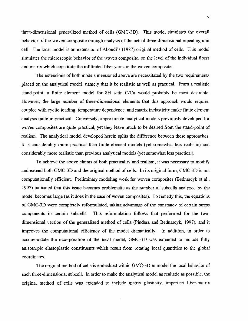
The extensions of both models mentioned above are necessitated by the two requirements

placed on the analytical model, namely that it be realistic as well as practical. From a realistic

stand-point, a finite element model for 8H satin C/Cu would probably be most desirable.

However, the large number of three-dimensional elements that this approach would require,

coupled with cyclic loading, temperature dependence, and matrix inelasticity make finite element

analysis quite impractical. Conversely, approximate analytical models previously developed for

woven composites are quite practical, yet they leave much to be desired from the stand-point of

realism. The analytical model developed herein splits the difference between these approaches.

It is considerably more practical than finite element models (yet somewhat less realistic) and

considerably more realistic than previous analytical models (yet somewhat less practical).

To achieve the above claims of both practicality and realism, it was necessary to modifL

and extend both GMC-3D and the original method of cells. In its original form, GMC-3D is not

computationally efficient. Preliminary modeling work for woven composites (Bednarcyk et al.,

1997) indicated that this issue becomes problematic as the number of subcells analyzed by the

model becomes large (as it does in the case of woven composites). To remedy this, the equations

of GMC-3D were completely reformulated, taking advantage of the constancy of certain stress

components in certain subcells. This reformulation follows that performed for the two-

dimensional version of the generalized method of cells (Pindera and Bednarcyk, 1997), and it

improves the computational efficiency of the model dramatically. In addition, in order to

accommodate the incorporation of the local model, GMC-3D was extended to include fully

anisotropic elastoplastic constituents which result from rotating local quantities to the global

coordinates.

The original method of cells is embedded within GMC-3D to model the local behavior of

each three-dimensional subcell. In order to make the analytical model as realistic as possible, the

original method of cells was extended to include matrix plasticity, imperfect fiber-matrix

bonding, and consistent (Brayshaw) averaging to allow the model to simulate the transversely

isotropic behavior of a unidirectional composite (Brayshaw, 1994). While each of these features

had been previously incorporated in the original method of cells independently, they had not

previously been combined.

Thus, an analytical model for woven metal matrix composites is developed which is both

realistic and practical. This model is called Woven Composites Generalized Method of Cells

(WCGMC). The model is versatile and can simulate a wide range of thermomechanical loading

conditions for woven and braided composites. Herein, WCGMC is employed to simulate the

mechanical behavior of 8-harness (8H) satin carbodcopper (CICu). This woven metal matrix

composite is a candidate for high heat flux applications. An extensive experimental investigation

into the mechanical behavior of 8H satin CICu was performed by Bednarcyk et al. (1997), the

results of which are summarized in Chapter 4 of this report. A parametric study is performed

with the model to highlight the effects of geometric unit cell refinement, fiber volume fraction,

porosity, residual stresses, and imperfect fiber-matrix bonding on the mechanical response of 8H

satin CICu. Model predictions are then compared with the experimental data for the composite

to evaluate the accuracy of the model and identify areas for improvement.

2. Analytical Model - WCGMC

The analytical micromechanics model developed in this investigation is called woven

composites generalized method of cells (WCGMC). It is based on an embedded approach in

which a local micromechanics model, the original method of cells, is embedded in a global

micromechanics model, the three-dimensional generalized method of cells (GMC-3D). This is

shown schematically in Figure 2.1. GMC-3D uses an arbitrary number of homogeneous three-

dimensional subcells to represent the three-dimensional repeating unit cell of a material. In

WCGMC, the equations of GMC-3D are used, but the three-dimensional subcells are permitted

to be heterogeneous and thus able to represent a portion of an infiltrated fiber yarn. This subcell

heterogeneity is accomplished by using the original method of cells to model the local behavior

of the three-dimensional subcells. In addition, matrix plasticity, Brayshaw averaging (to allow

the infiltrated yarn subcells to exhibit transversely isotropic behavior) (Brayshaw, 1994), and

imperfect fiber-matrix bonding are incorporated in WCGMC on the local level in the embedded

original method of cells. In order to provide WCGMC with the level of computational efficiency

Figure

. . . . * - . . . . . * -

I

I I __C

Schematic representation of the incorporation of composite subcells into GMC-3D via the original method of cells.

necessary to simulate the thermo-inelastic behavior of a sufficiently refined woven composite

unit cell geometry, it was necessary to reformulate the basic equations of GMC-3D. The

resulting global equations used in WCGMC represent a reduction of nearly sixteen times in the

number of unknown global quantities that must be determined in the model. The original

formulation of the GMC-3D equations will be presented first, followed by the reformulation, and

finally by the local equations for the subcell behavior.

2.1 GMC3D - Original Formulation

For a complete derivation of the equations for GMC-3D,. see Aboudi (1994). The

geometry considered by the model is shown in Figure 2.2. A multi-phase material is represented

by a parallelepiped unit cell which repeats infinitely in the three mutually orthogonal directions.

The cell is divided into an arbitrary number of parallelepiped subcells, each denoted by the three

indices (a py) . The total number of subcells in each direction is denoted by N , , Np, and N , .

Figure 2.2. GMC-3D geometry.

The displacement field in each subcell is assumed to be linear in the local subcell

coordinates, (x!"), Xj", T!')), centered in the middle of each subcell,

u(aflr) = w(aflr) + Q),!@Y) + y i B ) X ! ~ ) + dy) !aPy), I I (2.1)

where the subcell rnicrovariables, 4ja'y), p), determine the displacement field

dependence on each subcell coordinate. The subcell strain components are given by the usual

lunematic relations,

(ah) + ,yY)) Ca'y) = -(, ,

E g 2 J" i , j = 1,2,3. (2.2)

Because the displacement field is assumed to be linear, equation (2.1), the strain components

within each subcell are constant, and the average strain components for the unit cell are given by

the volume average of the strain components in the subcells,

Note that in order to simplify notation, summations over the indices ( a ~ y ) will be expressed as

in equation (2.3) above. That is,

Since the subcell strain components are constant within each subcell, the stress

components in each subcell are constant as well. The subcell stress components are related to the

subcell strain components by the subcell constitutive equations,

where are the subcell plastic strain components, aLMy) are the subcell coefficients of

thermal expansion (CTEs), and AT is the temperature change from a reference temperature. The

average stress components in the unit cell are given by the volume average of the subcell stress

components,

Continuity of displacements and tractions is required between subcells within the unit

cell, and between the unit cell and adjacent unit cells. These continuity requirements are

imposed in an average sense, that is the integrals of the appropriate displacement and traction

components along the appropriate boundaries are required to be continuous. Imposing the

displacement continuity conditions (see Aboudi (1994) for details) gives rise to six continuum

equations of the form,

These continuum equations form a system of equations which can be expressed as,

AG E, = J E , (2.13)

- - - where, E = {El E~~ ,533 2223 2213 2E12) , and E, is the 6 N, N p Ny - order subcell strain

vector given by E, = (r(l1') ... E ( ~ ~ N p "I), where each vector E ( ~ ~ ~ ) consists of the six subcell

strain components. AG contains cell geometric dimensions only, and it is an

[ N , (Np + Ny + 1) + Np(Ny + 1) + Ny ] x 6 N, Np Ny matrix. J contains cell dimensions, and it is an

[N, (Ng + Ny + 1) + Np(Ny + 1) + Ny ] x 6 matrix.

Imposing the traction continuity and using (2.5) gives rise to the system of equations,

A~(E,-E,P- AT) = 0 , (2.14)

where E! and a: are 6 N, Ng Ny - order subcell plastic strain and subcell CTE vectors, similar

in composition to E .. The matrix AM is 6 N , N, N y - ( N , N , + N , Ny + N , N , ) -

( N , + N p + N, ) x 6 N a N,N, and contains the subcell stifhess components. Combining (2.14)

and (2.13) yields,

A a s -a(&: AT AT) = KE,

where, = [ A ~ ] fi = [*dl] , K = [:I. Equation (215) can be solved for E, , A,

where, A = X-' K and D = X-I a . If the matrices A and D are partitioned into N , N~ N , sixth-

order square submatrices such that A = , then equation (2.16)

implies that,

E(a,r) = E + I)(@,) (E! + A AT) .

This equation gives the strain components in each subcell in terms of the applied cell strains, the

subcell plastic and thermal strains, and two concentration matrices, A ( ~ ) and D(,&).

Substituting (2.17) into (2.5) yields,

o(4y)=~(aar)[A(4r)~+~(@y)(~:+a,~~)-(~p(@y)+a(@y)~~)], (2.18)

and using the average stress equations (2.6), the elements of the effective elastoplastic thermo-

mechanical constitutive equation,

- o = c*(E-EP -a* AT) , (2.19)

can be found. The effective elastic stiffness matrix is,

the cell plastic strain vector is,

the average CTE vector is,

5 is the average stress vector, and E is the imposed average strain vector.

In this formulation of GMC-3D, the subcell strain components, given by equation (2.17),

serve as the basic unknown quantities. Since there are six unknown strain components per

subcell, the total number of unknown quantities which must be determined is 6 N , Np N, .

Determining these quantities (i.e., employing equation (2.17)) involves inverting the

6 Na N , N, x 6 Na N p Ny A matrix. In the presence of plasticity, the thermomechanical

loading must be applied incrementally, and an iterative solution procedure must be employed at

each load level (see Section 2.6). Thus, for a given thermomechanical loading simulation, the

unknown subcell strain components must be determined, and the A matrix must be inverted,

hundreds or thousands of times. As the number of subcells in the repeating unit cell becomes

large, the original formulation of GMC-3D becomes increasingly computationally inefficient.

For this reason, the GMC-3D equations have been reformulated so that sufficiently refined

woven composite unit cells can be modeled.

2.2 GMC3D - Reformulation

Since the individual subcells in WCGMC are heterogeneous, the subcells in GMC-3D

must be anisotropic. The subcell anisotropic constitutive equations can be expressed as,

The subcell traction continuity conditions require that, at subcell and unit cell interfaces, the

tractions be continuous. Since the unit cell and the subcells are parallelepipeds, each interface is

normal to one coordinate axis. Thus, each unit normal vector for each interface is parallel to one

coordinate axis, and particular subcell stress components (all of which are constant within a

subcell) are equal to the traction components at the interfaces. That is,

This allows each traction continuity condition to be expressed in terms of one subcell stress

component. In fact, the traction continuity conditions whch are applicable to the normal subcell

stress components require that each normal stress component be constant through all subcells

which are adjacent in the coordinate direction of that subcell stress component. That is, for

example, is constant when following a row of subcells through the unit cell shown in

Figure 2.2 in the x , -direction. This condition can be expressed as,

where ~ ( y ) has been introduced to denote the 11 stress component in each row of subcells

which are adjacent in the x, -direction. Similarly, for the remaining normal subcell stress

components,

,(as') = ( 4 2 ) = '""7' = q\@) . 33 O 3 3 . a a = 033 (2.27)

The traction continuity conditions which affect the shear stress components can similarly

be applied. One difference is that, by nature of the symmetry of the stress tensor (i.e. a, = aji) ,

two traction continuity conditions affect each subcell shear stress component. For example,

o!?) is constant when following a row of subcells which are adjacent in the x2 -direction, while

a\?) is constant when following a row of subcells which are adjacent in the x3-directions (see

Figure 2.2). However, since ogpy) = oksy), the 23 subcell stress component must be constant in

each layer of subcells with a constant value of a . This condition can be expressed as,

where 71;") has been introduced to denote the 23 stress component in each layer of subcells

which are adjacent in the x2 -direction or the x, -direction. Similarly, for the remaining subcell

shear stress components,

The utility of accounting for traction continuity in this explicit manner is clear. There are

only NP N y + Na N , + N, N p + N, + N p + N , unique subcell stress components, which have

been denoted <'I. Thus, if these subcell stress components, rather than the 6 N , N,N, subcell

strain components, are employed as the basic unknowns, the number of unknown quantities is

reduced substantially. This reduction in unknowns results in greater computational efficiency for

the model.

Substituting for the subcell stress components in the subcell constitutive equations (2.23)

using equations (2.25) - (2.30), solving for the subcell total strains, and substituting into the

continuum equations (2.7) - (2.12) yields,

These equations can be assembled into a global equation in matrix form and written,

e ~ = f ~ AT-fP, (2.37)

where c is an N B N y + N , Nr + N , N p + N , + NP + N y -order square matrix containing subcell

dimensions and subcell compliance components, T is an N p N y + N a N , + N u N B + N , + N B + N , -

order vector containing the unknown subcell stresses, f m is an

NPNr + N,Ny + N , N p + N , + N p + N y -order vector containing cell dimensions and global (cell)

strains, f ' is an NpNr + N , N y + N , NP + N , + N p + N, - order vector containing subcell dimensions

and subcell coefficients of thermal expansion, and f p is an N p N y + N , N y + N,NB + N , + N p + N , -

order vector containing subcell dimensions and subcell plastic strain components. The structure

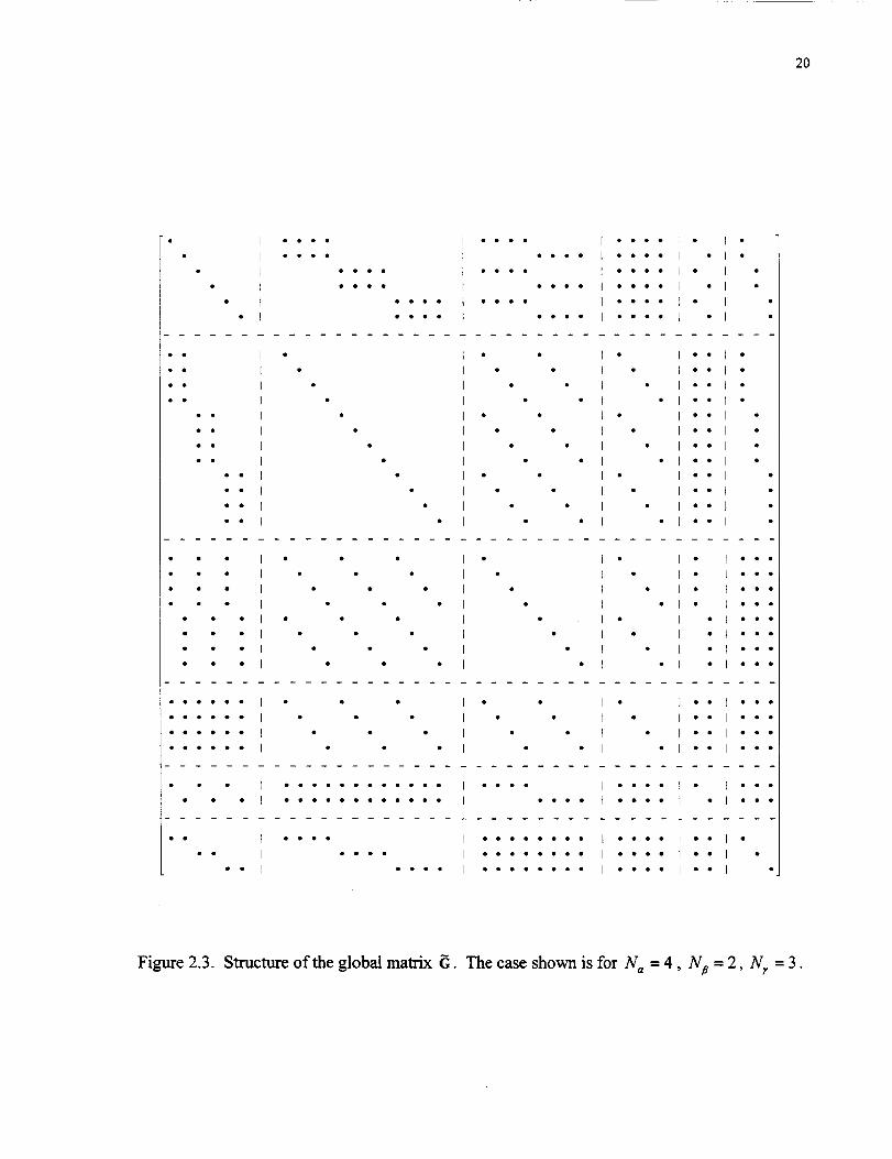
of the G matrix is shown in Figure 2.3. It consists of 36 submatrices, only 12 of which are fully

populated. The components of G , T , fm , f' , and f P are given in the appendix.

20

oooo

oooo

j oooe

I eooo

I oooo

I oooo

eeoo t oooo

oooo I oeoo

oooolo

oeo4 I •

oooo i •

9ooo I •

ooooIo

oooo I •

• • • n •

• • • n

• • • ]

I •

• I •

I

• I

• L

• I

...... I ° • • I • • I • I • ° I • o"

...... I • • ° I ° • / ° F "° I • • °• • • • • • I • ° • I • • I • I • • I • ° •

...... I • • • I ° • I ° n -- I • • •

• • • I • ........... I .... I .... I • E • • •• • ° I • .° o.°°° • • .. I • • .o I o°°° 1 • I • • °

• - I .... 1 °°. • .°°. I o°°° I • • I °• • I .... I ........ I .... 1 -o I °

° ° I ° • ° ° I • ° • • .... I .... I • • U •

Figure 2.3. Structure of the global matrix __,. The case shown is for N_ = 4, Np = 2, N r = 3.

To obtain explicit expressions for the subcell stress components, the global equation

(2.37) is inverted to obtain the subcell mixed concentration equation,

where the A!), B?), r~ x?) r~ , A(*), !I Q!), 'I-'!), T!), and 0;) terms are given in the appendix.

This equation is referred to as a mixed concentration equation because the local or subcell

stresses are related to the global or cell strains. The average stress equation (2.6), can now be

applied to the subcell stresses in equation (2.38), yielding,

The expressions for ) from equation (2.38) are substituted into equations (2.39). and the

results compared with the global (cell) constitutive equation,

to yield closed-fonn expressions for the cell effective stiffness components, c,; , the cell effective

coefficients of thermal expansion, a,, and the cell effective plastic strain components, 2;.

These expressions are,

c:, c:* c:3 c:4 c:5 c;6 c,', ci2 ci3 c; c,', c;

Thus, as was the case in equations (2.20) - (2.22) in the original formulation of GMC-3D,

equations (2.41) - (2.43) provide closed-form expressions for the effective thermoelastic

constants and effective plastic strain components for the three-dimensional unit cell. However,

comparing equations (2.17) and (2.38) shows that, for applied therrnomechanical loading, there

are far fewer unknown variables to be determined using the reformulated version of the GMC-3D

equations. This is clearly illustrated in Figure 2.4. The number of unknown variables is plotted

versus the number of subcells in the repeating unit cell to be analyzed for the case in which the

1 10 1 W loo0 IWOO 1 OOOOOO

Number of Subcells

Figure 2.4. Number of subcells vs. number of unknown variables for the original and reformulated versions of GMC-3D for N , = N p = N , .

number of subcells is identical in each direction. For 1,000,000 subcells, there are nearly 200

times fewer unknowns in the reformulated version compared to the original version.

2.3 Heterogeneous Subcells via the Reformulated Original Method of Cells with Imperfect Fiber-Matrix Bonding

In order to model a woven composite with GMC-3D, it is necessary for the three-

dimensional subcells to represent the infiltrated fiber yarns. This is achieved by allowing the

three-dimensional subcells to be heterogeneous, with unidirectional fibers. In WCGMC, the

fiber direction of the unidirectional composite comprising each three-dimensional subcell is

arbitrary, as are the fiber material, matrix material, fiber-matrix debonding parameters, and fiber

volume fraction. The unidirectional composite in each subcell is modeled in its principal

material coordinates by the original method of cells, also developed by Aboudi (1987) (see

Figure 2.1).

One feature of the original method of cells is that it simulates a unidirectional composite

consisting of an isotropic matrix and a transversely isotropic fiber as cubic rather than

transversely isotropic. hat is, the effective stiffness matrix of such a composite as determined

by the original method of cells has six independent components when it should have five. In

order to model the unidirectional composite as transversely isotropic, Aboudi (1 987) suggested

averaging the effective stiffness components in the transverse plane of symmetry. This

procedure indeed provides transversely isotropic elastic behavior, but Brayshaw (1 994) showed

that it leads to an inconsistency in the unit cell stress components. That is, the weighted sum of

the subcell stress components is not equal to the average stress components in the unit cell. The

correction of this inconsistency is imperative when the original method of cells is embedded in a

global micromechanics model because the average stress components for the original method of

cells unit cell are continuously exchanged between the two models. Hence, Brayshaw's

averaging procedure, which eliminates the inconsistency was employed in WCGMC and will be

described in Section 2.4.

Since CICu composites are known to exhibit imperfect fiber-matrix bonding, this feature

was included in WCGMC on the local level in the original method of cells. The original method

of cells equations for composites with imperfect bonding were provided by Aboudi (1988), and

the consistent formulation for the original method of cells equations with perfect bonding was

provided by Brayshaw (1994). However, the combination of imperfect bonding and the

consistent formulation using the equations provided by the aforementioned authors proved

unmanageable. Thus, a different approach was taken. The equations of the original method of

cells were reformulated along the lines of the GMC-3D reformulation. This original method of

cells reformulation amounts to a specialization of the reformulation of GMC-2D presented by

Pindera and Bednarcyk (1997), with the additional features of imperfect bonding and Brayshaw

averaging. As will be shown, the reformulated equations of the original method of cells lend

themselves to the inclusion of imperfect bonding and consistent averaging.

The original method of cells provides effective constitutive equations for the two-

dimensional rectangular unit cell shown in Figure 2.5 consisting of three rectangular matrix

- Fiber

h , q a HJ Matr ix I h i I

L---x3 Repeating Unit Cell I ' ' x3

Figure 2.5. Original method of cells geometry.

subcells and one rectangular fiber subcell. Each subcell in the original method of cells is denoted

by the two indices ( p y ). These constitutive equations, in turn, describe the average response of

the subcells in GMC-3D. It is important to distinguish between the subcell indicial notation used

in the original method of cells ( f l y ) and that used in GMC-3D ( a h ). Though the notation is

similar, the indices refer to the subcell quantities in two distinct models. The procedure for

developing the effective constitutive relations in the original method of cells is similar to the

procedure used in GMC-3D: a first order displacement field is assumed for the subcells and

continuity of displacements and tractions between subcells and between cells is imposed in an

average sense.

Imperfect fiber-matrix bonding in the original method of cells is modeled by introducing

a discontinuity in the displacement components at the fiber-matrix interface. This displacement

discontinuity allows slippage or separation at the interface, and it can be characterized by a linear

relationship with the traction components at the interface (Aboudi, 1988). The discontinuity in

the displacement component normal to a given interface is related to the normal traction

component at the interface, while the tangential displacement discontinuity is related to the

tangential traction component at the interface. These two relations can be written,

['n], = Rnonl,, (2.44)

[a] , = R,O. I, (2.45)

where [u,], and [u,] , are the discontinuities, or "jumps" in the normal and tangential

displacements at the interface I, and R, and R, are the normal and tangential debonding

parameters. These parameters are, in effect, compliances of a flexible fiber-matrix interface, and

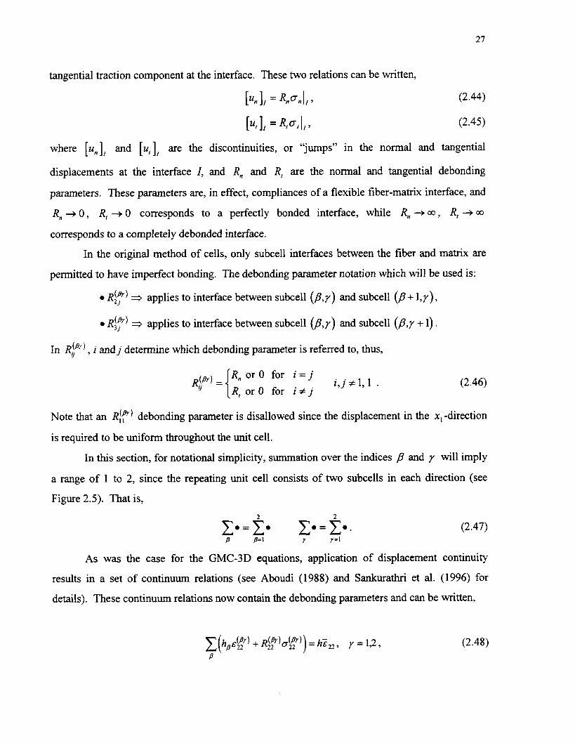
R, + 0 , R, -+ 0 corresponds to a perfectly bonded interface, while R,, + a, R, + oo corresponds to a completely debonded interface.

In the original method of cells, only subcell interfaces between the fiber and matrix are

permitted to have imperfect bonding. The debonding parameter notation which will be used is:

R(") s applies to interface between subcell (P, y ) and subcell (P + 1, y ) , 2 J . R(") a applies to interface between subcell (fly y ) and subcell (P,? + 1). 3 1

In R?) , i and j determine which debonding parameter is referred to, thus,

R, or 0 for i = j i , j # l , l .

R, or 0 for i + j

Note that an RIP) debonding parameter is disallowed since the displacement in the x, -direction

is required to be uniform throughout the unit cell.

In this section, for notational simplicity, summation over the indices P and y will imply

a range of 1 to 2, since the repeating unit cell consists of two subcells in each direction (see

Figure 2.5). That is,

As was the case for the GMC-3D equations, application of displacement continuity

results in a set of continuum relations (see Aboudi (1988) and Sankurathri et al. (1996) for

details). These continuum relations now contain the debonding parameters and can be written,

The normal constitutive equations for the homogenous subcells are,

where, Z,, is the uniform axial strain for all subcells, and E$") are the remaining normal

subcell strain components, alpy) are the subcell CTEs, cp) are the subcell plastic strain

components, SF) are the subcell compliance components, and * are the

subcell stress components. Solving this system of equations (2.50) for o\y) yields,

Substituting this expression (2.5 1) in the second and third subcell constitutive equations (2.50)

yields,

Substituting these equations (2.52) and (2.53) into the two continuum equations (2.48) and (2.49)

yields,

As was the case in GMC-3D, imposing continuity of normal tractions amounts to

requiring normal stress components to be constant in rows of subcells which are adjacent in the

appropriate normal direction. For the original method of cells, this is simpler since there are only

four subcells in the repeating unit cell. The normal traction continuity conditions can be

summarized as,

Through the use of these equations (2.56) and (2.57), along with the grouping of terms, equations

(2.54) and (2.55) can be written as,

where,

Examining the terms defined in equation (2.60) and (2.62) (which contain debonding

parameters), with the use of equation (2.46), it is found that,

In matrix form, equations (2.58) and (2.59) can be written,

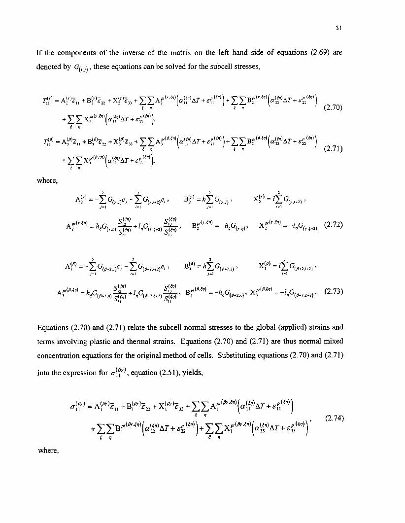
If the components of the inverse of the matrix on the left hand side of equations (2.69) are

denoted by G(,,,] , these equations can be solved for the subcell stresses,

Y - - Y 2 , I + B(r)2Y 2 + ~ ~ i z ~ ~ + ~ x A : f ( y " s ) ( n ~ ~ ~ A T + Eyl(b)) + c ~ ~ P ( Y , P ~ ) c v P s (2.70)

+ x ~ X r ( ~ . c ~ ) ( a ~ ~ ) A T + &P 33 ( ~ 7 ) ). 5 s

= ~ i p ) ~ ~ ~ + B ~ P ) z ~ ~ + x!P)z3, + ~ x ~ r ( ~ " ~ )

P s (2.71) + x x x $ " ~ ' ( ~ ! ~ A T + E : ~ ( ~ ) ,

5 s

where, 2 2 2 2

A:) = -x G~,,~)c, - ~ ( ~ , + ~ ) e , , BPI = h x G(~,,) Y

i=l j = I x?) = lx ~ ( ~ , i + 2 )

j i l i=l

A:(~,P" = h G s,'?' s , C ~ ) B ~ f ( ~ - c s ) = -h G Xp(rin) = -1 G r (7.7) + 'sG(r .c+2) 2 c (1.7) y s ( ~ . e + 2 )

(2.72) S, I

Equations (2.70) and (2.71) relate the subcell normal stresses to the global (applied) strains and

terms involving plastic and thermal strains. Equations (2.70) and (2.71) are thus normal mixed

concentration equations for the original method of cells. Substituting equations (2.70) and (2.71)

into the expression for oiy), equation (2.51), yields,

where,

The stress averaging equations require that the geometrically-weighted subcell stresses sum to

equal the global (cell) stresses,

Substituting the expressions for the subcell stresses, equations (2.70), (2.71), and (2.74), into the

averaging equations, (2.76), (2.77), and (2.78), and comparing with the form of the global (cell)

normal constitutive equation,

allows the identification of the effective normal stiffness components, C; , coefficients of thermal

expansion, a,, and plastic strain components, Z,P,

r 7

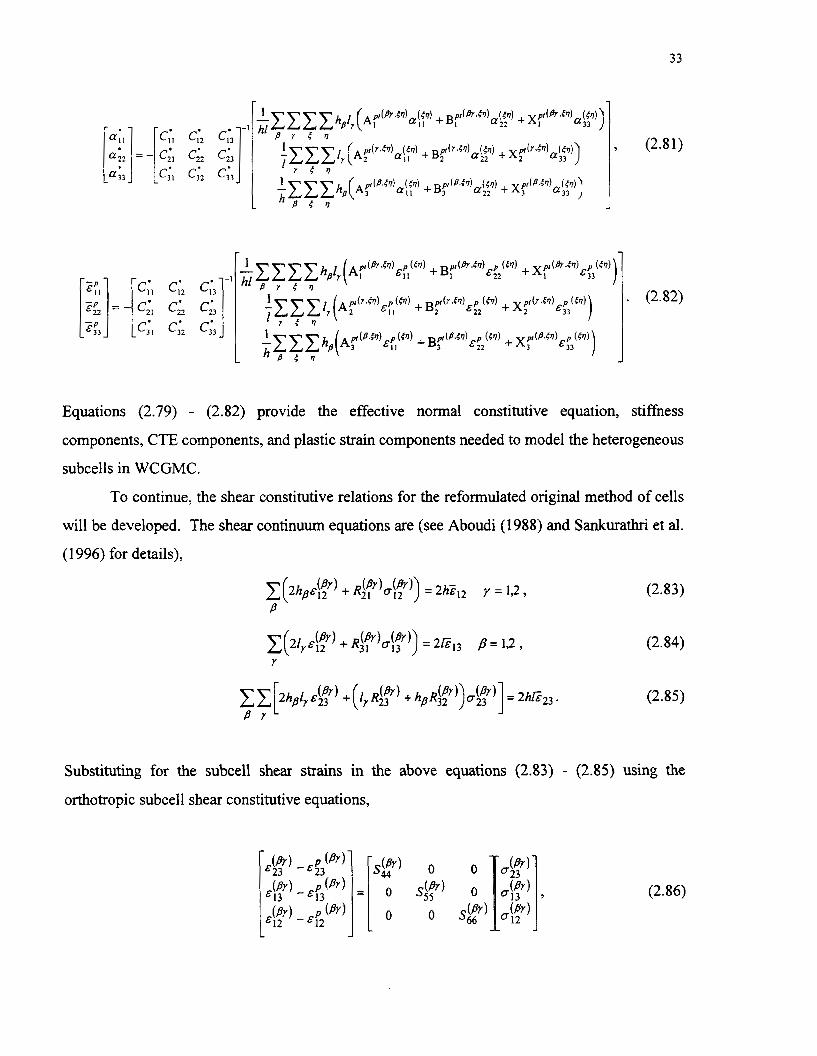
Equations (2.79) - (2.82) provide the effective normal constitutive equation, stiffhess

components, CTE components, and plastic strain components needed to model the heterogeneous

subcells in WCGMC.

To continue, the shear constitutive relations for the reformulated original method of cells

will be developed. The shear continuum equations are (see Aboudi (1988) and Sankurathri et al.

(1 996) for details),

Substituting for the subcell shear strains in the above equations (2.83) - (2.85) using the

orthotropic subcell shear constitutive equations,

and making use of the subcell shear traction continuity conditions, which can be written,

yields,

where,

Examining the debonding parameters in the above expressions (2.93) and using equation (2.46),

1 c (hp;?) + s @I) = h R Q I ) + il @I) + h ~ ( ~ 9 + i2 + 4 R::') + lI 4:') + 4 ~ : f ) + l2 @) 32 -+ - - - - (2.96)

B Y 4 4 R, o o R, o o

= 2(h1 +I , )R, .

Thus,

Equations (2.90) - (2.92) can be easily solved for the subcell shear stresses,

where,

Equations (2.98) - (2.100) relate the subcell shear stress components to the average (cell) strain

components and plastic terms. Thus, these equations are the shear mixed concentration

equations for the original method of cells.

The shear stress averaging equations,

can then be applied using equations (2.98) - (2,100) to yield,

Comparing these equations (2.107) - (2.109) to the global (cell) orthotropic shear constitutive

equations,

allows the identification of the cell effective shear stiffness components and plastic strain

components,

Thus, closed-form constitutive equations, (2.79) and (2.1 1 O), have been developed for the

original method of cells with imperfect fiber-matrix bonding. Note that the debonding

parameters appear only in the terms defined in equations (2.67), (2.68), and (2.97). Hence,

unlike the original formulation of the original method of cells, including imperfect bonding in the

reformulation amounts to simple modifications of a few equations.

In WCGMC, given the geometry and properties of the fibers and matrix that constitute

the unidirectional composites in each three-dimensional subcell, the reformulated original

method of cells is used to calculate effective thennoelastic properties for each three-dimensional

subcell in the principal material coordinates of the given three-dimensional subcell. An effective

stiffness matrix is then assembled for each three-dimensional subcell in the principal coordinates,

and this stiffness matrix is rotated in three dimensions to the coordinates of the three-dimensional

cell. The reformulated version of GMC-3D uses these effective stiffness matrices for each three-

dimensional subcell to determine the effective stiffness matrix and effective properties for the 3D

cell. If the woven composite is treated as purely elastic, this is all that is required. However, if

matrix plasticity is included, the formulation becomes more complex.

The subcell plastic strains are determined from the original method of cells in conjunction

with the classical incremental plasticity theory (see Section 2.5). The strains in each three-

dimensional subcell, known from the solution of the global constitutive equation (2.40), the

mixed concentration equations (2.38), and the subcell constitutive equations (2.23), represent the

average unit cell strains in the original method of cells. From these average unit cell strains,

stress and strain components for each of the four subcells can be determined via the original

method of cells mixed concentration equations and subcell constitutive equations. The

knowledge of these subcell stresses and strains allows the determination of plastic strains within

each original subcell using the classical incremental plasticity theory equations presented in

Section 2.5. These plastic strains are then used to determine global (cell) plastic strains in the

original method of cells via equations (2.82) and (2.1 12). These cell plastic strains are then

rotated back to the global coordinates, and then they represent the three-dimensional subcell

plastic strains for the three-dimensional subcell considered. The three-dimensional subcell

plastic strains are used to re-solve the global constitutive equation (2.40), for the entire three-

dimensional unit cell.

2.4 Brayshaw Averaging

When the original method of cells is used to model a unidirectional composite, one

subcell is occupied by the fiber material while the remaining three subcells are occupied by the

matrix material. In most cases, the fiber material is at most transversely isotropic (as in the case

of carbon fibers), while the matrix material is usually isotropic. In the form presented above, the

original method of cells represents such a composite as a cubic material when in fact it is

transversely isotropic. Aboudi (1987) overcame this problem by performing orientational

averaging of the effective stiffness matrix in the x2 - x3 plane (see Figure 2.5) to yield a

transversely isotropic effective stiffness matrix. This was done via the equation,

where c~(B) are the effective stiffness matrix components rotated by an angle 8 in the x2 - x3

plane, and d i is the resulting transversely isotropic effective stiffness matrix. Brayshaw (1994)

showed that the above averaging procedure results in an inconsistency in the stress concentration

composition. That is, the geometrically-weighted subcell stresses do not sum to the cell global

(cell) stresses as in equations (2.76) - (2.78) and (2.104) - (2.106).

Brayshaw showed that the inconsistency is eliminated if orientational averaging is

performed on stresses or strains rather than the effective stiffness terms. Further, it was

a IC determined that to ensure consistency, the integration limits should be -- to - rather than 0 to 4 4

IC . In the reformulated original method of cells, Brayshaw averaging may be performed directly

on the mixed concentration equations (2.70), (2.71), and (2.98) - (2.100). In the x2 - x, plane, the

rotation equations (which apply to both stresses and strains) are,

where c = cos6 and s = sin 8. Applying equation (2.1 14) to the subcell stresses yields,

The mixed concentration equations (2.70), (2.71), and (2.98) - (2.100) are then substituted into

the above equations for the un-primed subcell stresses, yielding, for example,

The rotation equation (2.1 15) is then applied to the global strains, 2, , thermal strains, n fn ) A T ,

and plastic strains, E&(") , in the equations for each rotated subcell stress of the form above. This

yields, for example,

4~)' = ( c 2 ~ t ) + S ~ A \ ~ ) ) Z , ,' + ( c 2 ~ ! j ) + s ~ B \ ~ ) ) ( c ~ Z ~ ~ ' + s 2 ~ 3 3 ' - 2 ~ ~ 2 ~ ~ ' )

'1 [ ( 2 (1) + s 2 ~ i p ) ) ( s 2 ~ 2 2 ' + c 2 ~ ~ ~ ' + 2 s ~ ~ ~ ~ + ZSCA s c ~ ~ ~ ' - scz3; + (c2 - s2 ) z ~ ~ ' ] + c X z

2 p t ( b " ) ) ( a ~ AT + &:, + x ~ ( C 2 A h ( r " q ) + s A3 5 rl '"I (2.122)

+ Z Z ( c 2 B f f i y 7 e " + s2Bff'd''")[c2(a\(*jAT + &P2 AT + &fpf] - 2 s c & f ~ c q f ] 5 0

Equations of the form above provide the rotated subcell stresses as a function of the global

strains, thermal strains, and plastic strains, all of which are rotated as well. These rotated sibcell

stresses can now be averaged according to Brayshaw by use of the equation,

This orientational averaging is performed for each subcell stress component to yield,

where,

and the constants arising due to integration are,

1 1 1 1 k 2 = - - - 3 1 , =-+-, 3 1 kl =-+-, k4 =---. (2.136)

2 K 2 A ) 3 8 7 r 8 K

The final step in the application of Brayshaw averaging involves simply replacing the

appropriate terms in equations (2.70), (2.71), and (2.98) - (2.100) with the hatted terms above.

Thus, the averaged global constitutive equations can be written as,

where the averaged effective stiffness components, coefficients of thermal expansion, and

global plastic strain components are, r 1

- - - 01 A 1 - 0 2 2 A -

0 3 3 A -

O 2 3 A

- O13 A

- - 0 ~ 2 -

- r 2 , 1

$,, %,,

%,,

- - - ' f l A

-P ' 2 2 A

-P '33 A

-P '23 A

6 3

-'12 -P

- -

-,

A .

-all- A .

a, A *

- a , , 0 0

0 -

> ' (2.137) AT-

- * ele e l o o o t , t2 t3 o o o e l Si2 o o o 0 0 0 0 0 0 0 0 e5 0

- 0 0 0 0 0 ei6

- -

o < % , ,

2.5 Classical Incremental Plasticity Theory

The equations for calculation of the subcell plastic strain increments in the original

method of cells subcells are here presented. The derivation follows that of Mendelson (1983)

and simplifications provided by Williams and Pindera (1 994) and Williams (1 995). Omitting the

designation (by) that identifies a given subcell in the original method of cells for notational

simplicity, the subcell total strain components are given by the sum of the elastic strain

components, the plastic strain components, and the plastic strain increments,

E . . Y = se. Y + E$ +d&$. (2.143)

The modified total strain components are defined as,

&!. E 6.. -&P * Y Y r l (2.1 44)

Combining equations (2.143) and (2.144) yields,

E! . = &e +d&P. B Y Y (2.145)

The mean dilatation is subtracted fiom (2.145) to give,

where, ei and e$ are deviatoric quantities defined as shown. Hookeys elastic law is given by

where,

is the stress deviator, and the Prandtl-Reuss equations are given by,

d ~ ; = a> dA ,

where, dA is the proportionality constant obtained fiom the consistency condition requiring that

the stress vector remains on the yield surface during plastic loading. Eliminating the deviatoric

stress using (2.147) and (2.149) yields,

and substituting for e$ in equation (2.146) using (2.1 50) yields,

eb= ( I + - tG1dl)dE!'

The equivalent modified total strain is defined as,

Eel Jj.e!.e!. Y Y .

Substituting for ei in equation (2.152) using (2.15 1) yields,

where the definition of the effective plastic strain increment, d&$ has been indicated.

Combining (2.15 1) and (2.153) to eliminate the term ( I +A) yields,

which, upon rearrangement, becomes,

It can be shown that the proportionality constant, d l , can be expressed as,

where,

is the effective stress. Substituting for d;l in equation (2.153) using (2.156) results in, - =eff d~' -- eff 3G ' (2.158)

and substituting for d&& in equation (2.155) using (2.158) yields,

dill

where a modified proportionality constant, dA1, has been defined.

The plastic strain increments for the subcells in the original method of cells are calculated

from equation (2.159). This equation represents a modification of the Prandtl-Reuss equations

(2.149), such that the plastic strain increments are calculated from the modified total strain

deviator rather than fiom the stress deviator. This form allows better convergence when it is

employed in an iterative solution procedure. The terms in equation (2.159) are calculated from,

where,

where E, H ~ ~ , and a, are the elastic modulus, hardening slope, and yield stress for the material

based on a bilinear stress-strain response.

2.6 Solution Procedure in the Presence of Plasticity

The objective of the analytical model is to predict the inelastic response of a material

exhibiting periodic microstructure when subjected to global mechanical loading and a

temperature change. This is done via the effective constitutive equation (2.40). In the present

model, mechanical loading is imposed as global strain components, E d . The effective stifmess

components, Ci, and effective CTE components, a;, are determined from closed-form

expressions involving the repeating unit cell geometry, the subcell compliance components, and

the subcell CTEs. The compliance components and the CTEs of the heterogeneous subcells are

determined using the original method of cells (see Section 2.3). One or more of the global strain

components, E V , are known fiom the imposed mechanical loading. The unimposed global strain

components are calculated from the effective constitutive equation (2.40) with the use of global

stress-free conditions. That is, for example, if E , , is applied, typically ad = 0 for i j # 1 1 .

When plasticity is present, the global constitutive equation (2.40) is nonlinear, and thus

cannot be solved for the global stresses, 5, , directly. The nonlinearity arises because the global

plastic strain components, %, depend on the subcell plastic strain components, E ; ' ~ ' ~ ) , which

themselves depend implicitly on the subcell stress and strain components. The subcell stress

and strain components can only be determined once the global constitutive equation is solved.

Thus, to solve for the global stress components, Zg, iteration is necessary to find the correct Zp

for the imposed E . In addition, the mechanical loading in the form of imposed global strains, E ,

as well as any thermal loading, must be applied in an incremental manner.

p(aPY) The three-dimensional subcell plastic strain components, E~ , are calculated from the

local subcell plastic strain components in the original method of cells, E:'"). At a given

magnitude of the thermomechanical loading, these local plastic strains are expressed as the local

plastic strains at the previous thermomechanical load plus an increment in the local plastic strains

due to the increment in the thermomechanical load. This procedure was outlined by Mendelson

(1 983) and can be summarized as,

where d ~ f " ) are the increments in the subcell plastic main components calculated using the

original method of cells in conjunction with the classical incremental plasticity theory (Section

2.5). Thus, once the local plastic strain increments are determined, the local plastic strains

follow from equation (2.162), and the three-dimensional subcell plastic strains, upon which the

unknown global plastic strains depend, can be calculated as well.

The iterative procedure actually used in the model allows equation (2.40) to be bypassed

during iteration. The mixed concentration equation (2.38) is used instead. The subcell and

global stresses are calculated after convergence has occurred for a particular loading increment

and are not active in the iteration procedure. The iterative procedure may be outlined as follows:

Apply a loading increment (i.e., a small increase in temperature or strain).

Estimate the local plastic strains from equation (2.162).

Determine the three-dimensional subcell plastic strains using the original method of cells and determine the plastic terms in (2.38) from the equations in the appendix.

Obtain the stresses in each three-dimensional subcell from equation (2.38).

Determine three-dimensional subcell strains from the subcell constitutive equations (2.23).

Apply these subcell strains to the original method of cells, from which new estimates of the local plastic strain increments are determined through the use of equation (2.159).

Update the local plastic strains with equation (2.162) using the new local plastic strain increment values.

Check for convergence of the local plastic strains.

If convergence has been achieved, calculate the global stresses from equation (2.40) and go to step 1.

If convergence has not been achieved, go to step 3.

3. Modeling the Mechanical Response of 8H Satin C/Cu

In this chapter, predictions of WCGMC (described in the previous chapter) are presented.

In particular, the effects of unit cell microstructure and fiber volume fraction, porosity, residual

stresses, and imperfect fiber-matrix bonding on the predicted monotonic tensile, compressive,

and shear response of 8H satin CICu are examined. The effects are investigated in order to

determine which are important and how each alters the model predictions. Those effects that are

important will then be employed in Chapter 4 as the model predictions are compared with

experiment.

3.1 Effect of Unit Cell Microstructure and Fiber Volume Fraction

One benefit of using WCGMC to model woven composites is the geometric flexibility

offered by the embedded approach. As long as a repeating unit cell can be identified for a given

heterogeneous material, the micro-scale geometry can be discretized into parallelepiped subcells

and modeled with WCGMC. In addition, the averaged continuity conditions employed by the

method of cells make precise geometric representation less important than it is for numerical

finite-element or boundary-element models. It has been shown (Wilt, 1995) that for similar

geometrical representations, the two-dimensional version of the generalized method of cells

(GMC-2D) with 49 subcells matched elastoplastic finite-element predictions obtained using a

1088 element mesh. For the above cases, the CPU time for the fmite element model execution

was 3550 times that required for GMC-2D execution.

The geometry of the repeating unit cells for woven composites are often quite complex.

The weave of fiber yams is inherently three-dimensional, and each different weave type has a

different repeating unit cell (see Figure 1.3, for example). For an 8H satin weave, the repeating

unit cell is shown (from above) in Figure 3.1. The unit cell is large, encompassing eight yarns in

each of the two directions, but it is the smallest rectangular repeating unit cell for this type of

weave. A slightly smaller repeating unit cell can be identified if the rectangular shape

requirement is relaxed, but for implementation in WCGMC, the unit cell must be a

parallelepiped.

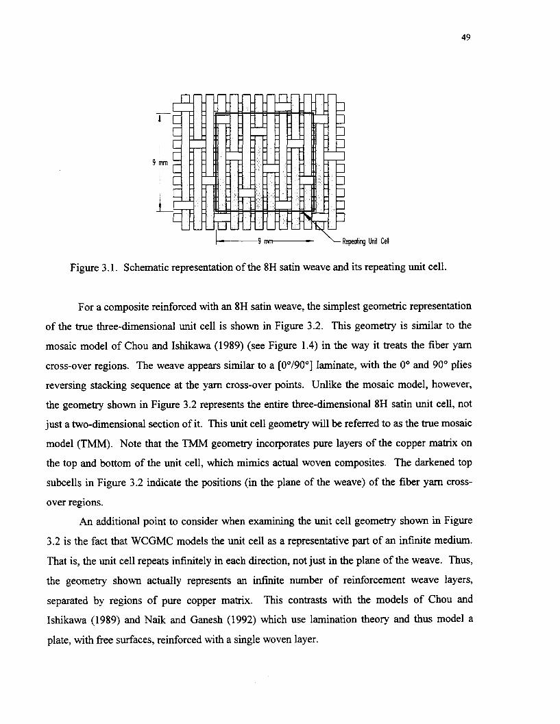
9 rnrn

I

Unit Cell

Figure 3.1. Schematic representation of the 8H satin weave and its repeating unit cell.

For a composite reinforced with an 8H satin weave, the simplest geometric representation

of the true three-dimensional unit cell is shown in Figure 3.2. This geometry is similar to the

mosaic model of Chou and Ishikawa (1989) (see Figure 1.4) in the way it treats the fiber yarn

cross-over regions. The weave appears similar to a [0°/900] laminate, with the 0" and 90" plies

reversing stacking sequence at the yam cross-over points. Unlike the mosaic model, however,

the geometry shown in Figure 3.2 represents the entire three-dimensional 8H satin unit cell, not

just a two-dimensional section of it. This unit cell geometry will be referred to as the true mosaic

model (TMM). Note that the TMM geometry incorporates pure layers of the copper matrix on

the top and bottom of the unit cell, which mimics actual woven composites. The darkened top

subcells in Figure 3.2 indicate the positions (in the plane of the weave) of the fiber yarn cross-

over regions.

An additional point to consider when examining the unit cell geometry shown in Figure

3.2 is the fact that WCGMC models the unit cell as a representative part of an infinite medium.

That is, the unit cell repeats infinitely in each direction, not just in the plane of the weave. Thus,

the geometry shown actually represents an infinite number of reinforcement weave layers,

separated by regions of pure copper matrix. This contrasts with the models of Chou and

Ishikawa (1989) and Naik and Ganesh (1992) which use lamination theory and thus model a

plate, with fiee surfaces, reinforced with a single woven layer.

The unit cell geometry shown in Figure 3.2 includes pure matrix layers above and below

the weave, but no other regions of pure matrix. Thus, in order to vary the overall fiber volume

fraction of the woven composite independently of the fiber volume fraction of the yam subcells,

the thickness of the pure matrix layers is varied with respect to the weave subcell thickness. That

is, the ratio x/h defined in Figure 3.2 is varied. Choice of the dimension w is arbitrary. In

addition, the TMM geometry lacks fiber continuity at the yam cross-over points. In order to

allow more freedom in varying the fiber volume fraction, as well as a more accurate

representation of the yarn cross-over geometry, a unit cell with considerably more subcells must

be employed. Figure 3.3(a) and (b) show the next level of refinement for the 8H satin composite

unit cell geometry. The unit cell geometry shown in Figun 3.3(a) is referred to as the continuous

mosaic model (CMM), and the unit cell geometry shown in Figure 3.3(b), which explicitly

includes rotated fibers in the cross-over regions, is called the directionally continuous mosaic

model (DCMM).

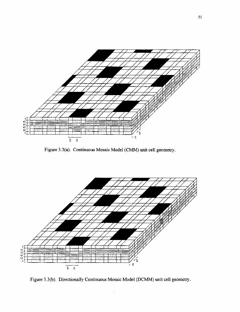
Figure 3.3(a). Continuous Mosaic Model (CMM) unit cell geometry.

Figure 3.3(b). Directionally Continuous Mosaic Model (DCMM) unit cell geometry.

Clearly, the CMM and DCMM geometries provide superior representation of the woven

composite compared to the TMM geometry. In addition, the CMM and DCMM geometries

include pure matrix subcells within the reinforcement weave as well as those located in the top

and bottom layers of the unit cell. This allows an additional geometric degree of freedom when

tailoring the subcell dimensions to provide a particular overall fiber volume fraction. However,

these refinements come at a computational cost. The TMM unit cell is comprised of 256 subcells

( 8 x 8 ~ 6 ) ~ while the CMM and DCMM unit cells are each comprised of 1536 subcells (16x 16x6).

For implementation in WCGMC these numbers can be reduced to 192 (8~8x3) and 1280

(16x16~5) by combining the top pure matrix layer of the unit cell with the bottom pure matrix

layer of the unit cell above the unit cell being considered. WCGMC execution times are

sensitive to the number of subcells comprising the unit cell considered. Indeed, prior to the

reformulation of GMC-3D, the DCMM geometry could not be employed for elastoplastic

simulations due to the large memory requirements and execution times required by the model

(see Bednarcyk et al., 1997). However, the reformulation of the equations of GMC-3D has now

made possible the use of the DCMM geometry for thermoinelastic modeling of woven metal

matrix composites.

For modeling 8H satin CICu, the fiber volume fraction of the fiber yarn subcells was

taken to be 65%. This value was determined via microscopic examination of actual C/Cu

specimens and represents an average for many infiltrated yarns in many composite specimens.

Given the fiber volume fraction of the infiltrated fiber yarns, the dimensions in the unit ceIIs may

be selected to obtain the desired overall fiber volume fraction. Table 3.1 provides the

dimensions for the microstructures that will be considered. Note that results generated using the

CMM geometry will not be presented since its microstructural accuracy is superseded by the

DCMM geometry. In addition, macroscopic results generated using the CMM geometry are

invariably nearly identical to those generated using the DCMM geometry (assuming the

dimensions are the same). Two versions of the DCMM geometry will be considered, each with a

different pure copper layer thickness. The DCMM #2 geometry is employed because of the

upper bound of 43.3% on the overall fiber volume fraction using the DCMM #1 geometry. Both

DCMM geometries model the actual microstructure of the 8H satin CICu composite specimens

reasonably realistically.

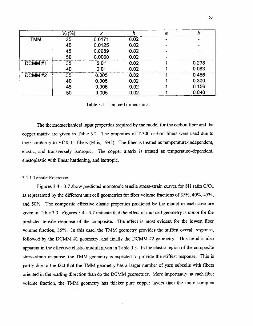
Table 3.1. Unit cell dimensions.

TMM

.......................................................................... DCMM #1

.............................................................. DCMM #2

The thermomechanical input properties required by the model for the carbon fiber and the

copper matrix are given in Table 3.2. The properties of T-300 carbon fibers were used due to

their similarity to VCX- 1 1 fibers (Ellis, 1995). The fiber is treated as temperature-independent,

elastic, and transversely isotropic. The copper matrix is treated as temperature-dependent,

elastoplastic with linear hardening, and isotropic.

Vf (%) x h a b 35 0.0171 0.02 - - 40 0.0125 0.02 - - 45 0.0089 0.02 - - 50 0.0060 0.02 - - - ......................................... 35 0.01 0.02 1 0.238 40 0.01 0.02 1 0.083 .......................................... 35 0.005 0.02 1 0.486 40 0.005 0.02 1 0.300 45 0.005 0.02 1 0.156 50 0.005 0.02 1 0.040

3.1.1 Tensile Response

Figures 3.4 - 3.7 show predicted monotonic tensile stress-strain curves for 8H satin C/Cu

as represented by the different unit cell geometries for fiber volume fractions of 35%, 40%, 45%,

and 50%. The composite effective elastic properties predicted by the model in each case are

given in Table 3.3. Figures 3.4 - 3.7 indicate that the effect of unit cell geometry is minor for the

predicted tensile response of the composite. The effect is most evident for the lowest fiber

volume fraction, 35%. In this case, the TMM geometry provides the stiffest overall response,

followed by the DCMM #1 geometry, and finally the DCMM #2 geometry. This trend is also

apparent in the effective elastic moduli given in Table 3.3. In the elastic region of the composite

stress-strain response, the TMM geometry is expected to provide the stiffest response. This is

partly due to the fact that the TMM geometry has a larger number of yarn subcells with fibers

oriented in the loading direction than do the DCMM geometries. More importantly, at each fiber

volume fraction, the TMM geometry has thicker pure copper layers than the more complex

54

T-300 Carbon Fibers

OFHC Copper Temp E v a (Jv HSP

Source

(Msi) (1 0-6t°F) (ksi)

EA ET GA "A "T cr, a T (Msi) (Msi) (Msi) (1 0-~PF) (1 0-610~)

29.42 3.67 6.40 0.443 0.05 -0.389 5.556

1 1 1 1 1 2 2

Source 3 3 3 314 314

Table 3.2: Material properties for T-300 carbon fibers and OFHC copper. Sources: 1 - Derstine (1 988); 2 - Naik and Deo (1 992); 3 - Rocketdyne Materials Properties

Manual (1987); 4 - NASA Lewis Research Center (1992).

geometries. The stiffness of the pure copper is greater than the transverse stiffness of the carbon

fibers (see Table 3.2), and since a large percentage of the fibers are oriented transverse to the

loading direction, the thicker copper layers provide increased stiffness. The presence of the

thicker copper layers also explains the stiffer response of the DCMM #1 geometry in the elastic

region compared to the DCMM #2 geometry (see Table 3.2).

Once yielding occurs in a given subcell, the ''stifmess" of the copper in that subcell

decreases dramatically. Thus, once yielding has occurred, the transverse stiffhess of the elastic

fibers is greater than the ''stiffness" of the copper, and the pure copper layers become much less

important. Now it is the pure copper subcells within the layers of the unit cell which represent

Figure 3.4. Predicted tensile stress-strain curves for 8H satin C/Cu, Vf = 35%, using different unit cell geometries.

Strain (%)

Figure 3.5. Predicted tensile stress-strain curves for 8H satin C/Cu, Vf = 40%, using different unit cell geometries.

0 10 0.15

Strain (%)

Figure 3.6. Predicted tensile stress-strain curves for 8H satin CICu, Vf = 45%, using different unit cell geometries.

0.00 0 05 0.10 0.15 0.20 0.25 0.30

Strain (16)

Figure 3.7. Predicted tensile stress-strain curves for 8H satin CICu, Vf = 50%, using different unit cell geometries.

Table 3.3 Effective elastic constants predicted by WCGMC for 8H satin CICu.

Geometry TMM

............................................................................ DCMM #I

DCMM #2

the reinforcement weave that affect the behavior. After yielding, these pockets of pure copper

serve as weak links, and bring about a more compliant post-yield response. The TMM geometry

has no pure copper subcells within the weave and thus provides the stiffest post-yield response.

Comparing the dimension b in Table 3.1 for the DCMM #1 and #2 geometries indicates that the

pockets of pure copper are larger for the DCMM #2 geometry (see Figure 3.3b). Thus the

DCMM #1 geometry has smaller weak links, and it provides a stiffer post-yield response.

It is also apparent from Figures 3.4 - 3.7 that increasing the overall fiber volume fraction

decreases the differences between the stress-strain curves predicted using the TMM and DCMM

#2 geometries. As Figure 3.7 shows, these curves are essentially coincident for a fiber volume

fraction of 50%. This too is explained by the size of the pure copper layers for the elastic region,

and by the size of the weak link pure copper subcells for the post-yield region. The difference in

the size of the pure copper layers between the TMM and DCMM #2 geometries decreases as the

fiber volume fraction increases (see Table 3.1). Hence the tensile moduli predicted using the two

geometries become closer in magnitude. Also, the size of the pure copper subcells within the

reinforcement weave in the DCMM #2 geometry decreases with increasing fiber volume fraction

(see Table 3.1). This explains the better agreement between the TMM and DCMM #2

geometries at higher fiber volume hctions.

Comparing Figures 3.4 and 3.5, however, indicates that, in the post-yield region,

differences between the curves predicted using the DCMM #1 and DCMM #2 increase as the

vf (%) E (Msi) G (Msi) v 35 16.04 6.763 0.2692 40 15.62 6.734 0.2544 45 15.19 6.706 0.2386 50 14.76 6.677 0.221 5 ........................................................................................................................................................................... 35 15.69 6.759 0.2547 40 15.47 6.728 * 0.2480 ....................................................................................................................................................................................................... - ................................................. 35 15.37 6.759 0.2413 40 15.12 6.730 0.2323 45 14.88 6.700 0.2242 50 14.66 6.663 0.2171

fiber volume fraction is increased from 35% to 40%. This is because the difference between the

b dimensions of the two geometries is much greater for a fiber volume fiaction of 40% (see Table

3.1). Hence, the difference in the size of the weak link copper subcells is greater for the 40%

fiber volume fiaction, which is apparent in the predicted stress-strain curves. Since the relative

size of the pure copper layers does not change with fiber volume fraction for the DCMM #1 and

DCMM #2 geometries (see Table 3. l) , in the elastic region, increasing the fiber volume fraction

has almost no effect on the difference between the predictions of the these geometries.

3.1 .2 Shear Response

Figures 3.8 - 3.1 1 and Table 3.3 indicate that the unit cell geometry has a lesser effect on

the predicted elastic shear response of the composite than on the predicted elastic tensile

response. However, the effect of unit cell geometry is much more pronounced in the plastic

region of the predicted shear stress-strain response than is the case in tension. The differences

between the shear stress-strain curves predicted using the TMM and DCMM #2 geometries

I 8 -

= a 6 - t

000 0 05 0 I 0 0 15 0 20 0 25 0 30

Engineering Shear Strain (%)

Figure 3.8. Predicted shear stress-strain curves for 8H satin CICu, Vf = 35%, using different unit cell geometries.

/+TMM t DCMM #I

0 00 0 05 0 10 0 15 0.20 0 25 030

Engineering Shear Strain (?k)

Figure 3.9. Predicted shear stress-strain curves for 8H satin CICu, Vf = 40% using different unit cell geometries.

10 - I I

=. 1 a 6 - f a

L Q rn C 4 - U)

-c TMM

p-

OW 0 05 0 10 0 15 0 20 0 25 030

Engineering Shear Strain (%)

Figure 3.10. Predicted shear stress-strain curves for 8H satin CfCu, Vf = 45%, using different unit cell geometries.

0 00 0.05 0.10 0.15 0.20 0.25 0.30

Engineering Shear Strain 6)

Figure 3.1 1. Predicted shear stress-strain curves for 8H satin C/Cu, Vf = 50%, using different unit cell geometries.

decrease as the fiber volume fiaction increases, as was the case in tension. Differences between

the curves generated using the DCMM #1 and DCMM #2 geometries increase as the fiber

volume fiaction increases, which is also identical to the trend in the tensile predictions. Thus, the

effects of the unit cell geometry on the predicted shear response of 8H satin C/Cu are the same as

the effects on the predicted tensile response for the composite. The effects can also be explained

exactly as they were for the tensile response, namely by the thickness of the pure copper layers

for the elastic response, and by the size of the weak link pure copper subcells within the

reinforcement weave for the post-yield behavior.

In the elastic region, the shear modulus of pure copper is still greater than the axial shear

modulus of the carbon fiber, but only slightly so (6.96 Msi vs. 6.40 Msi). Thus, in the elastic

region, although the trend in stiffness based on geometry that was observed in tension is still

present (see Table 3.3), the effect is much less apparent. Once yielding occurs, the shear

modulus of copper drops as drastically as does the tensile modulus, however, the difference

between the post-yield shear "stiffness" of copper and the shear modulus of the elastic fiber is

much greater than difference between the post-yield "stifhess" of the copper and the transverse

tensile modulus of the fiber. Thus the magnitude of the effect of the unit cell geometry on the

predicted composite post-yield behavior (caused by the weak link copper subcells) is much

greater for shear loading than is the case for tension. As the figures and Table 3.3 indicate,

however, the qualitative effects are identical.

3.1.3 Summary of Fiber Volume Fraction Effects

The effect of altering the overall fiber volume fraction on the predicted tensile and shear

response of the composite using the DCMM #2 geometry is isolated in Figures 3.12 and 3.13.

Note that in the elastic portion of the predicted stress-strain curves, increasing the fiber volume

fiaction leads to a more compliant response, while in the post-yield region, increasing the fiber

volume fiaction leads to a stiffer response. These trends are due to the low transverse tensile

modulus and axial shear modulus of the carbon fibers (see Table 3.2). When the overall fiber

Figure 3.1 1. Predicted tensile stress-strain curves for 8H satin CICu for different fiber volume fractions using the DCMM #2 unit cell geometry.

10 -

I

* T

I

- - m 6 - d m

e, Fi L C 4 - V)

0.00 0 05 0 10 0 15 0 20 0 25 0 30

Engineering Shear Strain (%)

Figure 3.12. Predicted shear stress-strain curves for 8H satin CICu for different fiber volume fractions using the DCMM #2 unit cell geometry.

volume fraction of the unit cell is increased, the volume fraction of the pure matrix subcells

decreases, while the local fiber volume fiaction of the infiltrated fiber yarns remains constant.

Since many fiber yams are oriented transversely to the loading direction in tension, and the

transverse stiffness of the fibers is lower than that of pure copper, lowering the relative volume of

pure copper lowers the tensile stiffness in the elastic region. This is true for shear loading as

well, but since the axial shear modulus of the carbon fibers is only slightly lower than the shear

modulus of copper, the effect is small. Once yielding of the copper matrix occurs, the transverse

fibers are considerably stiffer in tension and shear than the plastically deforming copper. Thus,

in the post-yield region of the stress strain-curves, lowering relative volume of pure copper (and

thus increasing the overall fiber volume fraction) increases the stiffness. For reasons explained

previously, the effect on the elastic response is greater in tension, while the effect on the post-

yield response in greater in shear.

3.2 Effect of Porosity

It was shown in the previous report on 8H satin C/Cu (Bednarcyk et al., 1997) that the

composite plates fabricated for the investigation typically contained significant porosity. This

porosity was not present in the pure copper matrix regions, but rather within the infiltrated fiber

yarns. Microscopic investigation of the composite yarns revealed that this porosity typically

occupied approximately 7% to 14% of the volume of the infiltrated fiber yarns.

In order to model its effect on the response of the woven composite, the porosity was

treated via a reduction in the properties of the copper matrix within the infiltrated fiber yarns.

WCGMC was used to model the tensile response of pure copper with spherical void inclusions.

This porous copper was modeled using a total of 343 subcells ( 7 x 7 ~ 7 cube). The overall volume

fraction of the voids was set at 20% and then 40% so that a yarn subcell with a fiber volume

fraction of 65% infiltrated with these effective porous copper materials would have effective

porosities of 7% and 14%, respectively. Figure 3.13 shows the predicted tensile response of the

porous copper. The predicted response of copper with no voids and 10% porosity are plotted for

0.00 0 05 0.10 0 15 0.20 0 25 0 30

Strain (%)

Figure 3.13. Predicted tensile response for porous copper as a function of % porosity.

comparison. Clearly, porosity has a major effect on the predicted response of pure copper. Table

3.4 provides a comparison of the effective room temperature properties for the porous copper

determined by the model.

To model the effect of porosity on the response of 8H satin CICu, the effective properties

for the porous copper given in Table 3.4 can be used as input properties for the copper located

within the inf31trated yarn subcells in WCGMC. Figure 3.14 shows the predicted tensile

response of 40% 8H satin CICu with 7% and 14% porosity w i t h the infiltrated yarn subcells.

Table 3.4. Effective properties for porous copper determined by WCGMC.

25 -

void content 0 % 10 % 20 % 40 %

+0% yam poroslty 1

r i +7% yam porosity -a- 14% yam porosity

E (Msi) v G (Msi) Y (ksi) HSP (Ms~) 18.8 0.350 6.96 10.3 1.425 14.3 0.291 5.55 8.13 1.11 11.7 0.260 4.62 6.61 0.931 7.26 0.207 3.01 5.42 0.597

Strain (%)

Figure 3.14. Predicted tensile response for porous 8H satin C/Cu as a function of yarn subcell % porosity.

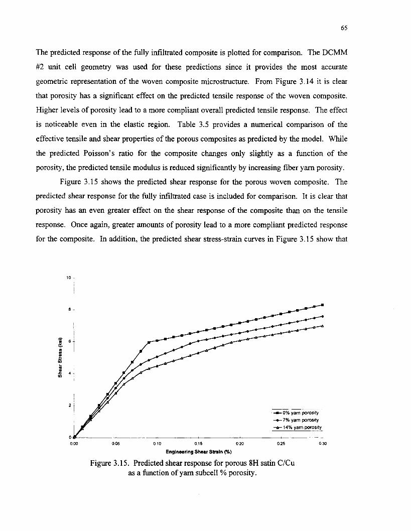
The predicted response of the fully infiltrated composite is plotted for comparison. The DCMM

#2 unit cell geometry was used for these predictions since it provides the most accurate

geometric representation of the woven composite microstructure. From Figure 3.14 it is clear

that porosity has a significant effect on the predicted tensile response of the woven composite.

Higher levels of porosity lead to a more compliant overall predicted tensile response. The effect

is noticeable even in the elastic region. Table 3.5 provides a numerical comparison of the

effective tensile and shear properties of the porous composites as predicted by the model. While

the predicted Poisson's ratio for the composite changes only slightly as a function of the

porosity, the predicted tensile modulus is reduced significantly by increasing fiber yam porosity.

Figure 3.15 shows the predicted shear response for the porous woven composite. The

predicted shear response for the fully infiltrated case is included for comparison. It is clear that

porosity has an even greater effect on the shear response of the composite than on the tensile

response. Once again, greater amounts of porosity lead to a more compliant predicted response

for the composite. In addition, the predicted shear stress-strain curves in Figure 3.1 5 show that

Engineering Shear Strain (X)

Figure 3.15. Predicted shear response for porous 8H satin CICu as a function of yarn subcell % porosity.

including yam porosity results in a much more gradual yielding of the composite compared to

the fully infiltrated case. Table 3.5 provides a numerical comparison of the effective shear

modulus for the porous composite. The data indicate that porosity, even when limited to the

infiltrated fiber yams, significantly reduces the overall stifhess of 8H satin CICu.

Table 3.5. Predicted effective properties for porous 40% 8H satin CICu.

yarn porosity 0 % 7 % 14 %

3.3 Effect of Residual Stresses

In order to model the effect of residual stresses on the predicted response of 8H satin

CICu, the cyclic capabilities of WCGMC were employed. Two loading cycles were

implemented. The first is a cool-down from a temperature at which the composite is assumed to

be globally and locally stress-free. This simulates the consolidation of the composite during

production. A high stress-fiee temperature (SFT), close to the melting temperature of copper

(1981 O F ) , would be chosen if the constitutive theory for copper modeled stress relaxation

accurately. In order to use incremental plasticity, a lower effective SFT should be chosen to

account for the relaxation of stresses in the copper matrix, which may occur at elevated

temperatures during the cool-down. After the cooldown, the simulated mechanical loading is

applied. During processing of the model predictions, the resulting mechanical stress-strain

curves are shifted such that, at the starting point for the mechanical loading, the global strain on

the composite is zero. ' h s simulates the assumed zero strain starting condition for mechanical

testing. Recall that the material properties of copper are temperature-dependent (see Table 3.2).

WCGMC uses linear interpolation between input temperatures to determine the mechanical

properties of the phases at the current temperature during thermal cyclic loading.

As mentioned above, at elevated temperatures, copper is subject to viscoplastic behavior

which can lead to relaxation of residual stresses. While the time-independent incremental

plasticity constitutive theory is realistic for copper at room temperature, it has been shown that,

E (Msi) G (Msi) v 15.12 6.730 0.2323 13.74 6.155 0.2170 12.76 5.541 0.21 10

for the elevated temperatures associated with composite fabrication, a time-dependent plasticity

theory should be employed (Bednarcyk and Pindera, 1996). One such viscoplasticity theory was

developed by Freed et al. (1994) specifically for copper, commonly known as Freed-Walker

viscoplasticity. While inclusion of Freed-Walker viscoplasticity in WCGMC is computationally

prohibitive (due to the stiff nature of the equations which must be integrated), a version of the

original method of cells embedded in classical lamination theory including this constitutive

theory was developed by Bednarcyk and Pindera (1 996).

In order to determine a reasonable range of SFTs for 8H satin CICu for use in WCGMC,

the aforementioned version of the inelastic lamination theory was employed to model the

globally stress-free cool-down from 1700 OF of a cross-ply CICu laminate with a fiber volume

fraction of 65% using the thermoelastic material properties given in Table 3.2. For the

viscoplastic material parameters of copper which were employed see Bednarcyk and Pindera

(1996). The cross-ply laminate provides the best simulation of an 8H satin composite possible

with lamination theory. A cool-down time of 900 seconds was employed to model the actual

cool-down of 8H satin CICu composites during fabrication. Results, in the form of a plot of the

effective stress in the matrix subcells in the plies vs. temperature are compared in Figure 3.16

with predictions in which the incremental plasticity theory was used to model the constitutive

behavior of the copper matrix. Note that, in this figure, the indices "12", "21", and "22" refer to

the matrix subcell py indices (see Figure 4.5).

Clearly, utilizing plasticity in conjunction with an SFT of 1700 O F vastly overpredicts the

stresses in a unidirectional CICu composite. Results generated using Freed-Walker

viscoplasticity indicate that a significant portion of the residual stresses predicted using

incremental plasticity are not actually present at room temperature. Although the exact values of

the residual stresses do not carry over from the cross-ply laminate to the woven composite, the

qualitative conclusion does: an SFT of 1700 OF is unrealistic for WCGMC.

In order to estimate a realistic value of the SFT for use in modeling 8H satin CICu,

additional simulations of the cool-down of 65% cross-ply CICu laminate were performed. For

these cases, the incremental plasticity constitutive theory was employed, and the SFT was varied.

The predicted residual effective stress after the cool-down is plotted vs. the SFT in Figure 3.17.

The SFT for which yielding does not occur during the cool-down is evident in this figure where

-Plasticity: 12 1 +Plasticity: 21 '

+Plasticity: 22

: + Freed-Walker: 12 : + Freed-Walker: 21

I + Freed-Walker: 22

0 600 800 1000 1200 1400 1600 leOO

Temperature (OF)

Figure 3.16. Effective stress in the subcells of a 65% volume fiaction cross-ply C/Cu composite as modeled by the original method of cells embedded in lamination theory with the Freed-Walker

viscoplasticity and incremental plasticity constitutive theories.

Stress-Free Temperature (OF)

Figure 3.17. Predicted residual stress in the subcells of a 65% cross-ply C/Cu laminate as a h c t i o n of SFT, where incremental plasticity theory has been employed.

the slopes of the plotted curves change abruptly. This temperature is between 150 OF and 200 OF.

Comparing Figure 3.17 with the Freed-Walker predictions in Figure 3.16, it is clear that in order

to obtain realistic estimates of the residual stresses in CICu composites using incremental

plasticity theory, an SFT lower than approximately 250 OF should be selected. This SFT is above

the minimum SFT that causes yielding in the composite upon cool-down, and it will be used as

an upper bound as the effect of varying the SFTs is investigated with WCGMC below.

Predicted thermal expansion curves for 8H satin CICu resulting from cool-down from

SFTs of 250 OF, 170 OF, and 120 OF are shown in Figure 3.18. Because of the low yield stress of

the copper matrix and the high axial CTE mismatch between the fiber and the matrix (see Table

3.2), the composite yields during simulated cooling from 250 OF. The composite remains elastic

during simulated cooling from 170 OF and 120 OF. For an SFT of 250 OF, Figure 3.18 shows that

by the time the composite reaches room temperature, the model predicts that it has undergone a

significant global thermal contraction. During cooling, the copper matrix is placed in tension,

while the carbon fibers are, for the most part, placed in compression. This is because the CTE of

-012 1

Temperature CF)

Figure 3.1 8. Predicted thermal expansion curves for 40% 8H satin CICu for cool-downs 250 OF, 170 OF, and 120 OF, to room temperature.

from

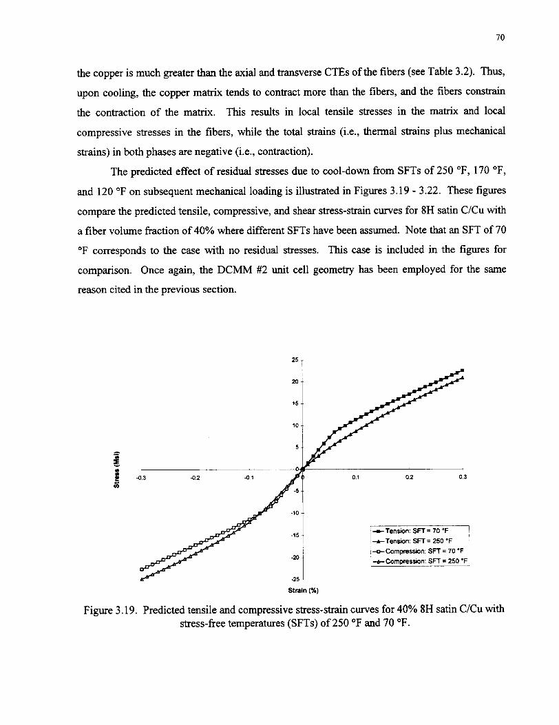
the copper is much greater than the axial and transverse CTEs of the fibers (see Table 3.2). Thus,

upon cooling, the copper matrix tends to contract more than the fibers, and the fibers constrain

the contraction of the matrix. This results in local tensile stresses in the matrix and local

compressive stresses in the fibers, while the total strains (i.e., thermal strains plus mechanical

strains) in both phases are negative (i.e., contraction).

The predicted effect of residual stresses due to cool-down from SFTs of 250 OF, 170 OF,

and 120 OF on subsequent mechanical loading is illustrated in Figures 3.19 - 3.22. These figures

compare the predicted tensile, compressive, and shear stress-strain curves for 8H satin C/Cu with

a fiber volume fraction of 40% where different SFTs have been assumed. Note that an SFT of 70

OF corresponds to the case with no residual stresses. This case is included in the figures for

comparison. Once again, the DCMM #2 unit cell geometry has been employed for the same

reason cited in the previous section.

Strain (%)

Figure 3.19. Predicted tensile and compressive stress-strain curves for 40% 8H satin C/Cu with stress-free temperatures (SFTs) of 250 OF and 70 O F .

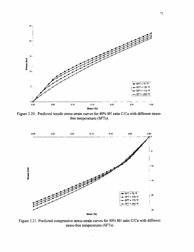
t SFT = 70 'F

\+SFT= 120 "F +SFT= 170'Fl

Strain (X)

Figure 3.20. Predicted tensile stress-strain curves for 40% 8H satin CICu with different stress- free temperatures (SFTs).

Strain (%)

Figure 3.21. Predicted compressive stress-strain curves for 40% 8H satin CICu with different stress-free temperatures (SFTs).

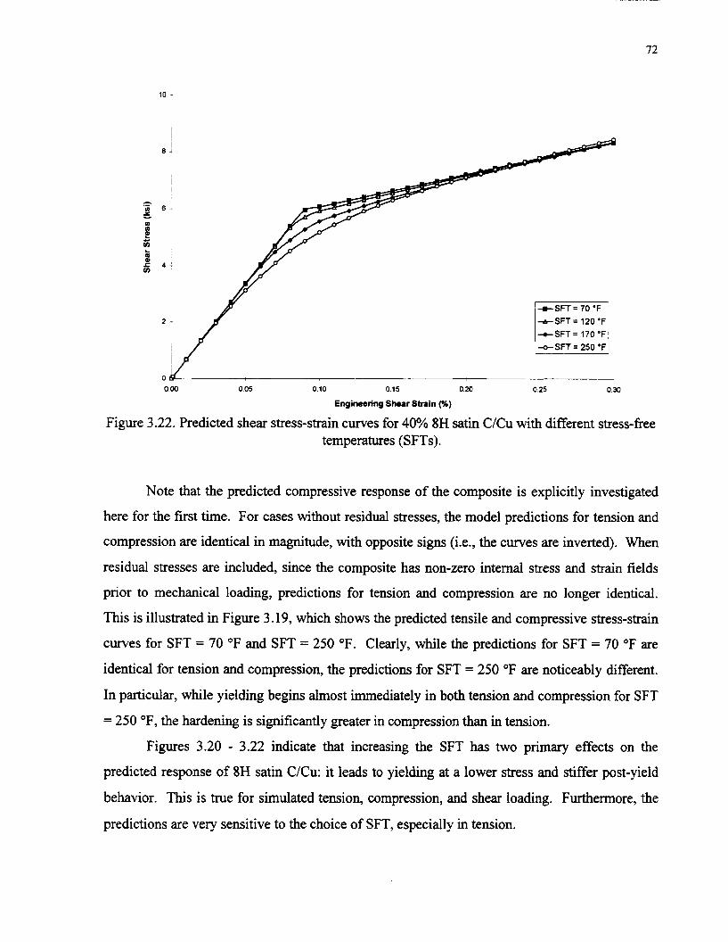
- - 0. W 0.05 0.10 0.15 0.20 0.25 0.30

Engineering Shear Strain (9C)

Figure 3.22. Predicted shear stress-strain curves for 40% 8H satin CICu with different stress-free temperatures (SFTs).

Note that the predicted compressive response of the composite is explicitly investigated

here for the first time. For cases without residual stresses, the model predictions for tension and

compression are identical in magnitude, with opposite signs (i.e., the curves are inverted). When

residual stresses are included, since the composite has non-zero internal stress and strain fields

prior to mechanical loading, predictions for tension and compression are no longer identical.

This is illustrated in Figure 3.19, which shows the predicted tensile and compressive stress-strain

curves for SFT = 70 OF and SFT = 250 OF. Clearly, while the predictions for SFT = 70 OF are

identical for tension and compression, the predictions for SFT = 250 OF are noticeably different.

In particular, while yielding begins almost immediately in both tension and compression for SFT

= 250 OF, the hardening is significantly greater in compression than in tension.

Figures 3.20 - 3.22 indicate that increasing the SFT has two primary effects on the

predicted response of 8H satin CICu: it leads to yielding at a lower stress and stiffer post-yield

behavior. This is true for simulated tension, compression, and shear loading. Furthermore, the

predictions are very sensitive to the choice of SFT, especially in tension.

In tension (see Figure 3.20), increasing the SFT fiom 70 OF to 120 OF decreases the

predicted yield stress of the composite noticeably, and raises the post-yield slope slightly. The

predicted yield stress is reduced further when the SFT is increased to 170°F. Recall that, upon

cooling fiom 120 O F and 170 OF, predictions indicated that the composite remains elastic. Thus,

upon initiation of simulated tensile loading, the composite still behaves elastically. For an SFT

250 OF, however, the composite yielded during the simulated cool-down. Thus, upon initiation

of simulated mechanical loading, regions of the composite are already "on" the yield surface, and

the composite exhibits plastic deformation immediately. The result is that the predicted initial

response of the composite is drastically changed for a relatively small change in the SFT. The

effect of varying the SFT on the predicted yield stress for the lower SFT values is equally

dramatic. It is also apparent from Figure 3.20 that increasing the SFT increases the predicted

tensile post-yield slope for the composite, but only slightly so. This results in the apparent

tendency of the predicted tensile stress-strain curves to converge at the higher strains.

Qualitatively, the compressive predictions, shown in Figure 3.21, resemble the tensile

predictions. Higher SFT causes lower predicted yield stresses and higher predicted post-yield

slopes. However, the effect on the initial slope of the predicted stress-strain curve is

considerably smaller in compression than in tension, while the effect on the post-yield behavior

is greater in compression than in tension. Thus the predicted stress-strain curves cross in Figure

3.2 1 while they do not cross in Figure 3.20.

As in tension and compression, the model predictions for the shear stress-strain response

of 8H satin C/Cu exhibit yielding at lower stresses and stiffer post-yield behavior as the SFT is

increased (see Figure 3.22). Varying the SFT between 70 OF and 250 OF has almost no effect on

the predicted initial shear response of the composite. However, as in tension, the predicted yield

stress is significantly reduced as the SFT is increased. As in compression, due to the higher post-

yield slopes associated with higher SFT, the predicted stress-strain curves cross, but they do so at

much higher levels of stress and strain.

The effects of varying the SFT discussed above can be explained by examining the

evolution of plastic strain in the subcells of the 8H satin C/Cu repeating unit cell during

simulated mechanical loading. Figure 3.23 is a plot of the predicted average effective plastic

0.00 0.05 0.10 0.15 0.20 0.25 0.30

Applied Global Tensile Strain (SC)

Figure 3.23. Predicted average effective plastic strain in several three-dimensional subcells as a h c t i o n of the applied global strain for SFTs of 250 OF and 70°F. The numbers on the plot

correspond to the subcells numbered in the diagram above.

strain in several subcells vs. the applied global strain for simulated tensile loading for SFTs of 70

OF and 250 OF. The diagram at the top of the figure identifies the subcells to which the curves in

the figure correspond. The particular subcells chosen, though all fiom the same cross-section of

the unit cell, are representative of most subcells in the repeating unit cell.

The reasons for the earlier yielding and stiffer post-yield behavior predicted in tension as

the SFT was increased are readily apparent in Figure 3.23. For an SFT of 250 OF, many subcells

have yielded during the cool-down and begin to accumulate additional plastic strain immediately

upon application of the simulated tensile loading. This contrasts with the curves that represent

an SFT of 70 OF which indicate that the subcells remains elastic (with zero plastic strain)

initially. As the SFT is increased fiom 70 OF, even if no subcells yield upon cool-down, residual

stresses in the subcells become greater. Thus, upon application of the simulated tensile loading,

certain subcells yield sooner, lowering the composite yield stress. This explanation is valid for

predicted compressive and shear results, which ehbi ted the identical trend in yield stress based

on SFT, as well.

The greater post-yield slopes which resulted fi-om increased SFTs can also be explained

via Figure 3.23. Certain subcells in the repeating unit cell (# 1, #3, and # 1 1) remain elastic to a

higher level of the applied global strain for an SFT of 250 OF compared to an SFT of 70 OF. B s

is because, after the simulated cool-down, the state of residual stress in the matrix of a given

subcell may be unfavorable for accumulation of plastic strain in response to the global loading.

That is, the global tensile loading may cause the state of stress in the subcell to pass through a

portion of the yield surface, and load elastically. This is, in effect, due to the highly non-uniform

state of residual stress and strain in the repeating unit cell that results fiom the simulated cool-

down, allowing a wide range of stress states in the subcells. Since some subcells load elastically

longer and accumulate plastic strain at a lower rate, higher SFT gives rise to stiffer post-yield

behavior. The reason for the increase in the post-yield stiffness as the SFT is increased for

compression and shear is identical.

Comparing the trends based on choice of SFT for tension and compression, it was

observed that the effect of SFT on yield stress is greater for tension than compression, while the

effect of SFT on the post-yield behavior was greater in compression than tension. Recall that,

after the simulated cool-down, the matrix in most subcells is in tension. Thus, upon application

of simulated global compression, many more subcells load elastically initially compared to

simulated global tension. Hence, for higher SFTs, the initial slope of the predicted compressive

stress-strain curve is not decreased significantly from the initial elastic slope of the predicted

compressive stress-strain curve for SFT = 70 OF. The curves in Figure 3.21 therefore do not

initially separate as much as those in Figure 3.20. However, since so many subcells do initially

load elastically for high SFT in compression, the stiffening effect on the post-yield behavior is

increased compared to tension.

The modeled effect of SFT on the shear response falls between the effects of SFT on

tension and compression. In shear, the effect of SFT on the predicted yield stress is greater than

the effect in compression, but not as dramatic as the effect in tension. Conversely, the effect of

SFT on the post-yield behavior is greater than the effect in tension, but smaller than the effect in

compression. This is because, since no in-plane shear stress arises in the composite during

simulated cool-down, the state of residual stress is not biased against plastic strain accumulation,

as was the case in compression. Thus, the large number of subcells which initially load

elastically that affect the predicted compressive response of the composite are absent during

simulated shear loading. However, upon application of the simulated shear loading, plastic strain

initially accumulates more slowly than in tension, also because the state of residual stress

involves no in-plane shear. This slow plastic strain accumulation rate causes the predicted shear

stress-strain curves in Figure 3.22 to nearly coincide initially, even for the SFT of 250 OF.

3.4 Effect of Imperfect Fiber-Matrix Bonding

Imperfect fiber-matrix bonding is incorporated in WCGMC on the local level, through

the original method of cells. Hence, the imperfect bonding that is modeled occurs between the

fibers and the matrix within the infiltrated fiber yams. As described in Section 2.3, the imperfect

fiber-matrix bonding is accounted for by a normal debonding parameter, R,, and a tangential

debonding parameter, R,. These parameters represent an effective compliance, in the two

directions, of the interface between the fiber and matrix in the original method of cells.

Debonding parameter values of zero correspond to a perfectly bonded interface, while as the

debonding parameters become large, total interfacial debonding is approached. The parameters

may be varied independently as well. For instance, if R,, = 0, and R, is large, the interface is

perfectly bonded in the normal direction, but completely debonded tangentially. This condition

corresponds to perfect sliding at the fiber-matrix interface (Aboudi, 1988).

3.4.1 Elastic Moduli

The effect of imperfect fiber-matrix bonding on the predicted elastic properties for 8H

satin C/Cu with a fiber volume fraction of 40% will be examined first. As before, the DCMM #2

unit cell geometry will be utilized for this purpose. Figures 3.24, 3.25, and 3.26 show the effects

of varying the debonding parameters on the predicted tensile modulus, shear modulus, and

Poisson's ratio of 8H satin C/Cu. In Figures 3.24 and 3.26, each curve corresponds to a constant

Figure 3.24. Predicted effective tensile modulus of 40% 8H satin C/Cu for different values of the debonding parameters R,, and R, .

Figure 3.25. Predicted effective shear modulus of 40% 8H satin C/Cu for different values of the debonding parameters R,, and R, .

Figure 3.26. Predicted effective Poisson's ratio of 40% 8H satin CICu for different values of the debonding parameters Rn and R, .

value of R,, given in the legend, while the value of Rn is varied along each curve. In figure

3.25, each curve corresponds to a constant value of R,, , given in the legend, while the value of

R, is varied along each curve. Figure 3.24 indicates that increasing either debonding parameter

results in a significantly lower effective tensile modulus of the composite. The most drastic

reduction in tensile modulus occurs when the debonding parameters are small, while as each

debonding parameter becomes large, the tensile modulus converges to a constant value. For the

fully debonded cases (i.e., R,, + w, R, + a) (not plotted in Figure 3.24), the predicted tensile

modulus for 40% 8H satin CICu is 1 1.12 Msi, which represents a reduction of 26.4% fiom the

perfectly bonded case. Clearly, imperfect fiber-matrix debonding can have a significant impact

on the predicted tensile modulus for 8H satin CICu. Figure 3.25 indicates that, while increasing

R, results in a significantly lower predicted shear modulus for 8H satin CICu, the normal

debonding parameter, R, , has no effect.

Figure 3.26 shows that the effect of increasing the normal debonding parameter on the

predicted Poisson's ratio for 8H satin C/Cu is similar to the effect on the predicted tensile

modulus. Namely, the Poisson's ratio is greatly reduced initially by increasing Rn and then

levels off as R, continues to increase. The effect of increasing R, on the predicted Poisson's

ratio is initially similar to the effect of increasing R, on the tensile modulus as well. However,

the predicted Poisson's ratio appears to converge to a constant value at a lower value of R, than

does the predicted tensile modulus. In addition, the predicted Poisson's ratio for R, = 5 x

first decreases, but then increases slightly as R, is increased from 5 x lo-' to 5 x 1 o6 . This

appears to be due to the fact that convergence of the predicted Poisson's ratio occurs at a lower

value of Rn as well, thus the curves in Figure 3.26 are, in effect, shifted to the left for the higher

R, values, compared to the curves in Figure 3.24.

The effect of R, on the normal behavior ofthe composite (including the effective tensile

modulus, shown in Figure 3.24) is mainly due to the averaging procedure employed in the

original method of cells (see Section 2.4). If Brayshaw averaging were not performed in the

original method of cells, the effects of the normal and tangential debonding parameters would be

completely decoupled for unidirectional composites. That is, the normal debonding parameter

would affect only the normal response of the unidirectional composite, while the tangential

debonding parameter would affect only the shear response. In the presence of rotated fibers,

however, the tangential and normal debonding effects will be linked when averaging is not

performed, but only in the plane of fiber rotation. That is, for fibers rotated in the xi - x j plane,

the normal and tangential debonding effects would be linked between the normal stresses o,, and

CT,. (no summations), and the shear stress ( r V . However, in the case of 8H satin CICu as

represented by the DCMM #2 geometry (see Figure 3.2(b)), all rotated fibers present are rotated

in the x , -x, and x , -x, planes. No fiber rotation is present in the plane of the weave, the x, - x ,

plane. Thus, for 8H satin C/Cu, without Brayshaw averaging, the effects of the normal and

tangential debonding would be expected to be decoupled for simulated in-plane shear loading.

For in-plane normal loading, since small out of plane shear stresses arise in some subcells, the

tangential debonding parameter would be expected to have a small effect.

Brayshaw averaging, in effect, links the debonding parameter effects for the in-plane

normal response and in-plane shear response. This can be seen clearly in equations (2.130) -

(2.133) and (2.137). The averaged terms which apply to the in-plane normal behavior in the

original method of cells, BY) , kipy), B: (m.h), kE"(".~v) 9 py) 3 3 3 k(h) B ~ ~ ( ~ ~ Y . c ? ) , and X3 , - p,(B~.t7)

are related to the un-averaged in-plane shear terms, A and A~"'", which are affected by the

tangential debonding parameter (see equations (2.104) and (2.98)). Hence, the normal response

of the composite (and thus the effective tensile modulus) is affected by R, . The effect of R, on

the normal response of 8H satin C/Cu is thus an artifact of the averaging procedure, rather than a

true effect of the sliding interface modeled by R, . However, since it affects the normal response

in the same way as does R,,, the utility of the compliant interface imperfect bonding model

should not be diminished by this fact.

It was observed in Figure 3.25 that R,, does not affect the predicted in-plane shear

modulus of the composite, even though Brayshaw averaging is employed. The reason for this

can be determined by once again examining the averaging equations. Equations (2.137), (2.73),

(2.74), (2.68), (2.69), and (2.70) show that, when Brayshaw averaging is performed, the averaged

in-plane shear terms, A(*) and 2'""' , are influenced by the un-averaged normal terms, which

are affected by the normal debonding parameter, R,, . However, the effect of R,, is identical for

the in-plane normal terms in the 2 and 3 directions. Examining equations (2.137) indicates that,

when this is the case, the effect of the normal debonding parameter on the averaged in-plane

shear terms, A(*) and A Apf(""), will subtract out due to the form of the equation. Thus, as was

observed in Figure 3.25, R,, does not affect the predicted in-plane shear response, which includes

the effective in-plane shear modulus, of the composite.

3.4.2 Mechanical Response

The effect of imperfect fiber-matrix bonding on the predicted tensile response of 40% 8H

satin C/Cu is shown in Figures 3.27, 3.28, and 3.29. In these figures, each curve represents the

predicted stress-strain response for a different value of R,, given in the legend. In each of the

three figures, a different value of R, was used; 0, 1 x lo", or 1. Using a value of 1 for either

0.10 0.15 0.20 0.25

Strain (I)

Figure 3.27. Predicted tensile stress-strain curves for 40% 8H satin C/Cu for different values of R,, with R, = 0.

0.M

Strain (X)

Figure 3.28. Predicted tensile stress-strain curves for 40% 8H satin C/Cu for different values of R, with R, = 1x lo-'.

0.00 0.05 0.10 0.15 0.20 0.25 0.30

Strain (%)

Figure 3.29. Predicted tensile stress-strain curves for 40% 8H satin C/Cu for different values R, with R, = l .

debonding parameter is large enough to correspond to the completely debonded case. These

figures indicate that the effect of increasing either debonding parameter on the predicted tensile

response of the composite is to significantly lower the elastic stiffness, yield point, and post-yield

stiffness.

Figure 3.30 shows the effect of imperfect fiber-matrix bonding on the predicted shear

response of 8H satin C/Cu. An R,, value of zero was used in this case, and R, was varied to

produce the three curves. As discussed earlier, R, does not affect the predicted in-plane shear

response of the composite. As the figure indicates, the effect of varying R, on the predicted

shear response of the composite is substantial; even greater than is the effect of varying R, on

the tensile response of the composite. In addition to the significant reduction of the predicted

shear modulus, yield point, and post-yield stiffness, increasing the tangential debonding

parameter smoothes out the yielding of the composite, making it less abrupt. The effect of R, on

the predicted shear response of the composite is greater than the effect of R, on the predicted

0 00 0 05 0 10 0.15 0.20 0.25 0 30

Engineering Shear Strain (%)

Figure 3.30. Predicted shear stress-strain curves for 40% 8H satin C/Cu for different values of R, with Rn = 0.

tensile response of the composite because, while R, only directly affects one half of the fiber

yarns (those oriented transverse to the loading directions), R, affects all of the fiber yarns.

3.5 Summary of Modeled Effects

Unit Cell Microstructure: Utilizing the more refined DCMM unit cell geometry gave rise to a

slightly more compliant overall predicted tensile response for 8H satin CICu compared to results

generated using the TMM geometry. The effect of unit cell refinement on the predicted elastic

shear response of the composite was similarly small, but the effect was much more significant on

the predicted shear post-yield response. This is due to the large difference between the axial

shear modulus of the carbon fibers and the post-yield shear "stiffness" of the copper matrix.

Fiber Volume Fraction: Increasing the overall fiber volume fraction of the composite gave rise

to a more compliant predicted elastic response, but a stiffer post-yield response in both tension

and shear. This is due to the drop in the effective "stiffness" of the copper associated with

yielding. Once again, the effect on the post-yield behavior was greater for shear than tension.

Porosiy: Increasing the porosity w i h n the infiltrated fiber yarns of 8H satin C/Cu gave rise to a

significantly more compliant overall predicted tensile response. The effect was qualitatively

similar, but of larger magnitude, for the predicted shear response of the composite.

Residual Stresses: Through utilization of a previously developed version of the original method

of cells embedded in lamination theory utilizing a viscoplastic theory, it was shown that for high

stress-fiee temperature (SFT) values, the model (based on incremental plasticity constitutive

theory) significantly overpredicts the residual stresses in the composite. In order to obtain

realistic residual stresses prior to simulated mechanical loading, it is necessary to use an SFT

below approximately 250 O F . Small changes in the SFT chosen for the composite had a

significant effect on the predicted mechanical response of 8H satin C/Cu. Higher SFT values

lead to lower predicted yield stresses for the composite, but stiffer post-yield behavior. The

effect on yield stress was greatest for simulated tensile loading and smallest for simulated

compressive loading, while the effect on the post-yield behavior was greatest for simulated

compressive loading and smallest for simulated tensile loading. For simulated shear loading, the

magnitudes of both effects were intermediate.

Imperfect Fiber-Matrix Bonding: Increasing either the normal or the tangential debonding

parameter produced a significantly more compliant overall predicted tensile response for 8H

satin C/Cu. Increasing the tangential debonding parameter produced a significantly more

compliant overall predicted shear response for the composite, while the normal debonding

parameter had no effect on the predicted shear response. The effect of the tangential debonding

parameter on the predicted shear response was greater than the effect of either debonding

parameter on the tensile response.

4. Model-Experiment Correlation

In this chapter, the mechanical test results for 8H satin C/Cu reported by Bednarcyk et al.

(1997) are summarized, and the predictions of the developed micromechanics model are

compared with the experimental data. Comparison is performed for monotonic and cyclic

tension, compression, and shear tests, as well as combined tension-compression and combined

compression-tension tests. By comparing the model to experimental data, the effectiveness and

accuracy of the model can be evaluated. Furthermore, by seeking the best possible agreement

with the model, additional insight can be gained on how and to what extent the previously

identified factors affect the actual behavior of the composite.

4.1 Summary of Experimental Results

For a complete presentation and discussion of the mechanical tests and results for 8H

satin C/Cu see Bednarcyk et al. (1997). Typical monotonic tensile and compressive stress-strain

curves for the composite are plotted in Figure 4.1 along with the stress-strain response of the

carbon fiber and the copper matrix. Note that, in tension, the composite is more compliant than

pure copper and yields at a lower stress as well. The composite response exhibits stiffening at

moderate strains and failed via breakage of the longitudinal fibers. In compression, the stress-

strain response of the composite is quite different. The initial compressive stiffness is somewhat

higher than the tensile stiffness, and the onset of yielding is more gradual in compression.

Compressive failure occurred via micro-buckling of the layers of the reinforcement weave,

resulting in a lower strength and strain to failure compared to tension. It should be noted that a

specialized compressive test fixture was used for the compressive (and combined) tests. Hence,

artifacts caused by this compressive fixture may be present.

Since the fiber-matrix bonding in C/Cu composites is poor, small amounts of titanium or

chromium were added to the matrix of some 8H satin C/Cu plates fabricated for the experimental

investigation. These alloying additions improve the wetting between the copper and the carbon

fiber and thus improve the bonding (Ellis, 1992; DeVincent, 1995). Previous work on C/Cu

composites indicated that the C/Cu - 0.7 wt. % Cr (C/Cu-Cr) composite would have the best

,,-%-- , - - - Fiber - trans.

/ .' -Failure (fiber breakage)

4 -Failure (rnicro-

budding) -Jo i

Strain (16)

Figure 4.1. Typical monotonic tension and monotonic compression response of 8H satin CICu-alloy composites.

fiber-matrix bonding, followed by the CICu - 0.5 wt. % Ti (CICu-Ti) composite, and finally by

the pure copper matrix (C/Cu) composite. By examining differences in the responses of the 8H

satin CICu composites with the three matrix alloy types, the effects of poor fiber-matrix bonding

can thus be examined.

The effect of matrix alloy type (and thus the effect of poor fiber-matrix bonding) on the

tensile and compressive response of 8H satin CICu is shown in Figure 4.2. In compression,

improved fiber-matrix bonding gives rise to a stiffer overall response. In tension, however, this

trend is reversed. The tensile response of the CICu-Cr composite, with its superior fiber-matrix

bonding, is most compliant.

The in-plane shear response of 8H satin CICu with the three different matrix alloy types

is shown in Figure 4.3. The shear test were of the Iosipescu type, employing a doubly-notched

specimen and a specialized test fixture (see Bednarcyk et al. (1997) for details). Shear yielding

occurred at low stresses, and a great deal of inelastic strain accumulated during the tests. Shear

tests were performed in displacement control and were stopped when contact of components of

I I

301

Strain (%)

Figure 4.2. Typical monotonic tension and monotonic compression stress-strain curves for 8H satin C/Cu-alloy specimens.

., 7

0 1 2 3 4 5 6 7 B 9 10

Engineering Shear Strain (%)

Figure 4.3. Typical monotonic shear stress-strain curves for 8H satin C/Cu-alloy specimens.

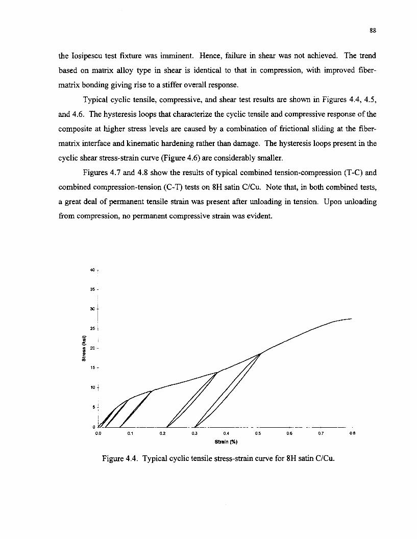
the Iosipescu test fixture was imminent. Hence, failure in shear was not achieved. The trend

based on matrix alloy type in shear is identical to that in compression, with improved fiber-

matrix bonding giving rise to a stiffer overall response.

Typical cyclic tensile, compressive, and shear test results are shown in Figures 4.4, 4.5,

and 4.6. The hysteresis loops that characterize the cyclic tensile and compressive response of the

composite at higher stress levels are caused by a combination of frictional sliding at the fiber-

matrix interface and kinematic hardening rather than damage. The hysteresis loops present in the

cyclic shear stress-strain curve (Figure 4.6) are considerably smaller.

Figures 4.7 and 4.8 show the results of typical combined tension-compression (T-C) and

combined compression-tension (C-T) tests on 8H satin CICu. Note that, in both combined tests,

a great deal of permanent tensile strain was present after unloading in tension. Upon unloading

from compression, no permanent compressive strain was evident.

0.0 0.1 0.2 0.3 0.4 0.5 0.6 0.7 0 8

Strain (%)

Figure 4.4. Typical cyclic tensile stress-strain curve for 8H satin CICu.

Strain (%)

Figure 4.5. Typical cyclic compressive stress-strain curve for 8H satin CICu.

8 +

7 - - I - n 6 *

- - ---- 1 2 3 4 5

Engineering Shear Strain v.)

Figure 4.6. Typical cyclic Iosipescu shear curve for 8H satin C/Cu.

-15 t

-m I Strain (%)

Figure 4.7. Typical combined tension-compression test results for 8H satin C/Cu.

-20 - S h i n (%)

Figure 4.8. Typical combined compression-tension test results for 8H satin C/Cu.

4.2 Monotonic Correlation

In order to realistically model the tensile, compressive, and shear stress-strain response of

8H satin C/Cu, it was desirable to use a well-refined geometric representation of the composite

unit cell. Thus the DCMM #2 geometry was employed. An overall fiber volume fraction of

40% was used for the simulations since this value is an approximate average for all 8H satin

C/Cu specimens, while an infiltrated yam fiber volume fraction of 65% was used. As was shown

in Section 3.1, small variations in fiber volume fraction should not have a significant effect on

the predicted elastic response of the composite. Furthermore, the effect of slight fiber volume

fraction variations (on the order of 1 % or 2 %) on the predicted post-yield behavior of the

composite are insignificant, compared to the scatter in the experimental results, as well.

Likewise, a yarn porosity of 14% was employed throughout the correlation simulations since this

value is realistic and representative.

For simulations of tests involving the compressive gripping apparatus (monotonic and

cyclic compressive tests and combined tests), a constraint on the lateral deformation of the

composite specimen was imposed. The test fixture used for these tests requires a specialized

non-dogboned specimen. The specimen is a rectangular plate measuring 1 inch by 4 inches, but

1 inch of either end is held rigidly in the gripping apparatus. This leaves only a 1 inch by 2

inches test section outside of the grips. It is suspected that, since the specimen is not dogboned

and the aspect ratio of the test section is small, the grips constrain the 8H satin C/Cu specimen

from expanding naturally in the in-plane direction transverse to the compressive loading.

WCGMC was used to model this grip constraint effect, when appropriate, by including a global

loading condition which, upon in-plane tensile or compressive normal loading, requires the

global mechanical strain component transverse to the loading direction to be zero, rather than the

stress component in the transverse direction (as is normally done). The effect of including this

grip constraint effect on the predicted monotonic compressive response of the composite is

shown in Figure 4.9. The constraint causes a slightly stiffer overall predicted response.

With the above model input parameters, as well as the temperature dependent fiber and

matrix material properties (see Table 3.2) fixed, three parameters remained to be chosen: the

debonding parameters, R, and R,, and the stress-free temperature. As shown in Sections 3.3

I - -25 Strain (%)

Figure 4.9. Predicted compressive stress-strain curves for 40% 8H satin C/Cu with and without the constraint effect from specimen gripping.

and 3.4, these parameters have a major impact on the model predictions, and thus must be chosen

carefully. In choosing realistic values of R,, and R, , the nature of the imperfect bonding model

must be considered. R,, and R, represent the normal and tangential compliances of an effective

interfacial layer (see Section 2.3) in the infiltrated fiber yams of the woven composite. Thus,

non-zero values of these parameters give rise to jumps in the displacement components at the

fiber-matrix interface which are proportional to the normal and shear stress components at the

interface. This compliant interface model is quite realistic for interfacial shear stresses. If a

positive or negative shear stress arises at an imperfectly bonded interface, a proportional jump in

a tangential displacement component results (governed by R). Thus, utilization of R, for

simulation of cyclic thermo-mechanical tests on 8H satin C/Cu is warranted.

Unfortunately, the compliant interface model is somewhat unrealistic for interfacial

normal stresses. If the interfacial normal stress is tensile, the model is representative, giving rise

to a positive jump in the displacement component normal to the interface. However, if the

interfacial normal stress is compressive, the compliant interface model breaks down. It now

predicts a negative jump in the normal displacement component at the poorly bonded interface,

when in fact, the interface should simply remain closed, with continuity of the normal

displacement component. Clearly, utilization of R, is unrealistic for simulated loading in which

fiber-matrix interfaces are placed in compression. In the case of 8H satin CICu as represented by

the DCMM #2 geometry, almost any simulated loading places some fiber-matrix interfaces in

compression. Furthermore, upon application of a simulated cool-down, the fiber-matrix

interfaces are placed in a state of residual compression since the CTE of copper is greater than

the transverse CTE of the fiber. Thus, even when the interface is placed in tension during

subsequent simulated mechanical loading, the interface should remain closed initially. In order

to keep the simulations as realistic as possible, an R, value of zero was used for all simulations,

disallowing the normal discontinuity in the displacement at the interfaces.

Recall from Section 3.4 that, due to the averaging procedure performed in the original

method of cells, R, does affect the normal response of the infiltrated fiber yarns. Thus, inclusion

of R, will have a noticeable effect on the tensile and compressive simulations. Furthermore, the

need for imperfect bonding in order to obtain reasonable model-experiment correlation in shear

was demonstrated by Bednarcyk et al. (1 997). In this report, preliminary shear predictions (made

by WCGMC) for perfectly bonding 8H satin C/Cu were shown to be in poor agreement with the

experimental results. In all cases, the model significantly overpredicted (by almost a factor of

two) the shear stress-strain response of the composite, while model predictions for tension and

compression were reasonable. Hence, the motivation for employing R, , but neglecting R, , is

clear. Since interfacial bonding is known to vary between the matrix alloy types, a different R,

value was employed for each. R, values of 2x lo-', 4x 1 0-', and 6x lo-' were used for the CICu-

Cr, CICu-Ti, and CICu composites, respectively. These values were chosen to provide

reasonable agreement with experimental shear results rather than experimental tensile or

compressive results because R, affects the shear response of the composite directly and most

significantly.

The remaining parameter to be chosen is the composite's stress-fiee temperature. As

shown in Section 3.3, utilization of a high stress-free temperature is unrealistic. Utilization of a

single stress-free temperature for all three matrix alloy types is unrealistic as well. It is likely

that, due to the different levels of imperfect fiber-matrix bonding, each matrix alloy type results

in a different stress-free temperature for the composite. Since the fiber-matrix bonding in the

C/Cu composite is inferior to that in the CICu-Cr composite, for example, residual stresses would

tend to relax to a larger extent since less restraint would be imposed by the fiber on the matrix.

This greater relaxation cannot be modeled well by the compliant interface debonding model

because it is caused predominantly by longitudinal displacement discontinuities between the

fiber and the matrix. That is, a jump occurs in the longitudinal (fiber direction) displacement

component at the poorly-bonded interface within the infiltrated fiber yarns. This is because the

large CTE mismatch between the fiber and the matrix in CICu occurs in the longitudinal

direction (8 .18~ 1 O ~ I O F vs. -0.389~ 1 0410~) rather than the transverse direction (8 .18~ 1 o-~/"F vs.

5 .556~10-~/"~) . The original method of cells treats the longitudmal displacement of the entire

infiltrated fiber yarn as constant, and the imperfect bonding model offers no jump in the

longitudinal displacement. Indeed, it was observed that choice of the debonding parameters had

little effect on the simulated cool-down for a given stress-free temperature.

Thus, it appears that the imperfect interfacial bonding model employed is insufficient to

realistically model the effect of imperfect bonding on residual stresses, necessitating the use of a

different stress-fiee temperature for each matrix alloy type. Values of stress-free temperature

were chosen to be realistic (as discussed in Section 3.3), to provide good correlation with

experiment, and to reflect the proper trend based on the degree of interfacial bonding for each

matrix alloy type (i.e., CICu-Cr has the highest stress-free temperature, while CICu has the

lowest). Stress-free temperatures of 170 OF, 120 OF, and 70 OF were utilized for CICu-Cr, CICu-

Ti, CICu, respectively. It is thus assumed here that the CICu composite is completely stress-free

at room temperature prior to mechanical loading. Though residual stresses in the CICu

composite are probably quite low, assuming that they are zero is a simplification.

Figure 4.10 compares the predicted tensile stress-strain response of 8H satin CICu-alloy

composites, where the parameters presented above have been used, with three experimental

tensile stress-strain curves for composites with each matrix alloy type. Clearly, the overall

correlation between model and experiment is acceptable. In the elastic region, the three

predicted stress-strain curves are nearly identical, and they agree well with the experimental

...'

Experiment: C/Cu-Ti

Experiment: CICu-Cr \+Rt = 6E-07. SFT = 70 'F I + Rt = 4507. SFT = 120 "F

Strain (%)

Figure 4.10. Comparison of model predictions (Vf = 40%) and experimental data for the monotonic tensile stress-strain response of 8H satin C/Cu-alloy composites.

curves. At the onset of yielding, the trend based on matrix alloy type is correctly predicted. The

simulated 8H satin C/Cu-Cr composite (R, = 2 x lo-' , SFT = 170 OF), yields first, followed by

the simulated 8H satin C/Cu-Ti composite (R, = 4x10'~, SFT = 120 OF), and finally by the

simulated 8H satin C/Cu composite ( R, = 6x SFT = 70 OF). This correctly predicted trend is

brought about by the stress-free temperatures chosen for the composites. As shown in Section

3.4, the trend in R, chosen for the composites would cause the opposite trend in yielding.

Hence, the effect of the poor interfacial bonding on the residual stresses in the composite (as

modeled by choice of stress-free temperature) dominates the trend based on matrix alloy type at

low strain. The direct effect of poor interfacial bonding on the predicted tensile response of the

composite is clearly overshadowed.

Examining the hardening behavior exhibited by the predicted tensile stress-strain curves

in Figure 4.10, it clear that the model predicts the opposite trend based on matrix alloy type

compared to the experimental results. As was shown in Section 3.3, employing a high SFT in

the model gives rise to a highly non-uniform residual stress states in the composite. Thus, during

the subsequent simulated tensile loading, a number of subcells have stress states that are initially

unfavorable for accumulation of additional plastic strain. The result is stiffer predicted post-yield

behavior as the SFT is increased. This effect works in concert with the direct effect of decreased

R, values, and as shown in Section 3.4, causes stiffer predicted post-yield behavior as well.

Thus, while the experimental tensile stress-strain curves for each matrix alloy type continue to

diverge at higher strains, the predicted curves converge. In order to compensate for this

discrepancy, a more realistic imperfect bonding model would be required.

Figure 4.1 1 compares the predicted compressive stress-strain response of 8H satin CICu-

alloy composites, with three experimental tensile stress-strain curves for composites with each

matrix alloy type. Again, the model parameters discussed earlier have been employed. Since

actual compressive tests were performed using the compressive gripping apparatus, the constraint

effect is included for the compressive simulations. Clearly, when the same parameters are used

- m t m t z I

I E x p e r i m e n t : ClCu-Cr 1 + ~ t = 6 ~ 4 7 . SFT = 70 'F I

+ Rt = 4E-07. SFT = 120 'F j

Strain (%)

-+- Rt = 2E-07. SFT = 170 'F

Figure 4.1 1. Comparison of model predictions (Vf = 40%) and experimental data for the monotonic compressive stress-strain response of 8H satin CICu-alloy composites.

I

- -25

to model compression as were used to model tension, the actual compressive response of the

composite is underpredicted. As was the case in tension, the predicted compressive stress-strain

curves are nearly identical in the elastic region. However, unlike the tensile predictions, the

compressive predictions are considerably more compliant initially than the experimental stress-

strain response. This is not because the compressive predictions are more compliant than the

tensile predictions. In fact, as was shown in Figure 4.9, the initial slope is greater in compression

than tension due to the constraint effect (in the case of R, = 6x10", SFT = 70 O F , the initial

slopes are 11.98 in tension, and 12.10 in compression). Rather, the discrepancy present in

compression is caused by the noticeably higher initial slopes in the experimental compressive

stress-strain curves compared to the experimental tensile stress-strain curves. Thus it appears

that, as modeled, the grip constraint effect is insufficient to account for the differences observed

in the initial stress-strain behavior of the composite between tension and compression. It is

likely that a more realistic imperfect fiber-matrix bonding model, which accounts for the closing

of the interface in compression, would account for some of the discrepancy. Recall that for these

simulations, the interface is treated as perfectly bonded in the normal direction, but imperfectly

bonded tangentially. Due to averaging, the tangential debonding does effect the predicted

normal response of the composite, but it affects the normal tensile and compressive identically.

Although the envelope of the predicted compressive stress-strain curves falls almost

completely below the envelope of the experimental compressive stress-strain curves in Figure

4.1 1, the correct trends in yielding and hardening are predicted by the model. That is, the

predicted compressive stress-strain curve for which R, = 6x lo", SFT = 70 OF, which models the

CICu composite, yields first (and hardens the least), followed by the prediction for R, = 4x lo-',

SFT = 120 OF, which models the CICu-Ti composite, and finally by the prediction for R, =

2x10-~, SFT = 170 OF, which models the C/Cu-Cr composite. Recall that these trends (in the

experimental stress-strain curves) are opposite to those observed in tension. Since both higher

values of R, and lower values of stress-free temperature give rise to earlier yielding and lower

post-yield slope (see Sections 3.3 and 3.4), this trend is expected. Thus, while the quantitative

correlation between model and experiment in compression is clearly inferior to that in tension,

the qualitative agreement is superior.

Figure 4.12 compares the predicted shear stress-strain response of 8H satin C/Cu-alloy

composites, with three experimental tensile stress-strain curves for composites with each matrix

alloy type. Clearly, as was the case in tension, the overall agreement between model and

experiment is acceptable. Unlike the predicted tensile and compressive stress-strain curves, in

the elastic region, noticeable differences exist between the three predicted shear stress-strain

curves. This is because the R, parameter has a much greater effect on the predicted shear

response of the composite than it does on the predicted tensile response and compressive

response. In addition, the correct trends in initial modulus, yield stress, and post-yield slope are

predicted by the model. That is, the predicted shear stress-strain curve for R, = 6x lo-', SFT = 70

OF, which models the CICu composite, is most compliant overall (i.e. appears lowest in the plot),

followed by the prediction for R, = 4x lo", SFT = 120 OF, which models the CICu-Ti composite,

and finally by the prediction for R, = 2x10-~, SFT = 170 O F , which models the CICu-Cr

composite. Recall from Sections 3.3 and 3.4 that while higher R, values give rise to a more

I

Experiment: CICu-TI

0 00 0 05 0 10 0 I 5 020 0 25 0 30

Engineering Shear Strain 6)

Figure 4.12. Comparison of model predictions (Vf = 40%) and experimental data for the monotonic shear stress-strain response of 8H satin C/Cu-alloy composites.

compliant overall shear response, higher stress-free temperatures cause yielding at lower stresses

and raise the post-yield slope in shear. Thus, it appears that, for shear, the direct effect of the

imperfect bonding (modeled via R, ) on yield stress dominates over the effect of the stress-free

temperature. Since this debonding model provides a level of quantitative as well as qualitative

correlation in shear that surpasses the correlation in both tension and compression, it can be

concluded that the imperfect bonding model is reasonably realistic for shear, while it somewhat

unrealistic for normal loading. It should be noted that, as the strain becomes large, and the

experimental shear stress-strain curves begin to flatten, the model tends to overpredict the post-

yield slope of the curves. This may be due to finite local strains or movement of the

reinforcement weave which cannot be simulated by the model.

4.3 Cyclic Correlation

The cyclic tensile, compressive, and shear stress-strain response of 8H satin C/Cu has

been simulated, as has the combined tension-compression and combined compression-tension

response. The cyclic response of only one matrix alloy type, Cu-Cr, has been modeled since the

important effects of matrix alloy type were addressed via simulation of the monotonic response

of the composite. In order to simulate the 8H satin C/Cu-Cr composite, as before, the parameters

R, = 2x 10'~ and SFT = 170 OF were employed. For cyclic compression, as well as combined

tension-compression and combined compression-tension, the grip constraint effect was included.

Other model parameters are identical to those used to generate the monotonic model predictions.

In the cyclic tension, compression, and shear simulations, unloading for each cycle was

performed at the identical strain at which unloading occurred in the actual tests being simulated.

Once the global stress during a given unloading cycle reached zero, the next loading cycle was

imposed.

Figure 4.13 compares the predicted cyclic tensile stress-strain response for 8H satin

CICu-Cr with experimental cyclic tension data. The model correlates reasonably well with

experiment, especially at the lower strains. However, the unloading portions of the stress-strain

curves indicate clearly that the model overpredicts the modulus of the composite, and the same is

true for the post-yield slope. Note (see Figure 4.10) that these discrepancies cany over fiom the

monotonic correlation. For both monotonic and cyclic loading of C/Cu-Cr, the fact that both the

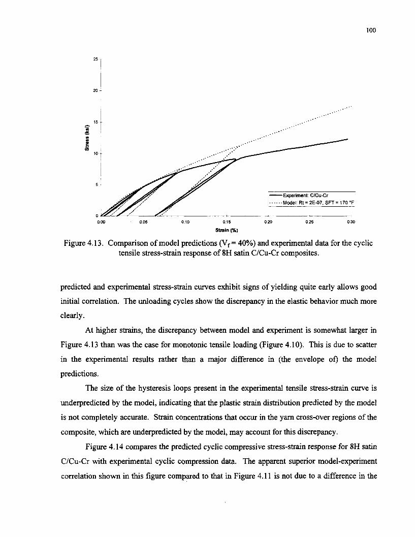
- ,- Experiment: CICu-Cr ...... Model: Rt = 2E-07. SF1 = 170 'F

0.00 0.05 0.10 0.15 0 20 0.25 0.30

Strain (%)

Figure 4.13. Comparison of model predictions (Vf = 40%) and experimental data for the cyclic tensile stress-strain response of 8H satin C/Cu-Cr composites.

predicted and experimental stress-strain curves exhibit signs of yielding quite early allows good

initial correlation. The unloading cycles show the discrepancy in the elastic behavior much more

clearly.

At higher strains, the discrepancy between model and experiment is somewhat larger in

Figure 4.13 than was the case for monotonic tensile loading (Figure 4.10). This is due to scatter

in the experimental results rather than a major difference in (the envelope of) the model

predictions.

The size of the hysteresis loops present in the experimental tensile stress-strain curve is

underpredicted by the model, indicating that the plastic strain distribution predicted by the model

is not completely accurate. Strain concentrations that occur in the yarn cross-over regions of the

composite, which are underpredicted by the model, may account for this discrepancy.

Figure 4.14 compares the predicted cyclic compressive stress-strain response for 8H satin

C/Cu-Cr with experimental cyclic compression data. The apparent superior model-experiment

correlation shown in this figure compared to that in Figure 4.11 is not due to a difference in the

envelope of the model predictions between the two figures. Rather it is due to scatter in the

experimental results. Though the predicted initial response of the composite is somewhat

obscured in Figure 4.14, it is in fact noticeable more compliant that the experimental initial

response. This is similar to the initial correlation for the monotonic compressive response. At

moderate strains, the envelopes of the predicted and experimental curves agree well, mainly due

to the fact that the envelope of the experimental curve falls somewhat below the average location

for CICu-Cr compressive stress-strain curves. As was the case in tension, the hysteretic behavior

of the composite is not well captured by the model, once again indicating a discrepancy in the

predicted plastic strain distribution for the composite.

Figure 4.15 compares the predicted cyclic shear stress-strain response for 8H satin CICu-

Cr with experimental cyclic shear data. Agreement between model and experiment is initially

quite good, but as yielding initiates, the model underpredicts the experimental response of the

composite somewhat. However, the post-yield shear behavior of the composite is overpredicted,

:-Experiment: ClCu-Cr I

...... Rt = 2E-07. SFT = 170 "F

- -25

Strain (#)

Figure 4.14. Comparison of model predictions (Vf = 40%) and experimental data for the cyclic compressive stress-strain response of 8H satin CICu-Cr composites.

0.0 0.1 0.2 0.3 0.4 0.5 0.6

Engineering Shear Strain (%)

Figure 4.15. Comparison of model predictions (V, = 40%) and experimental data for the cyclic shear stress-strain response of 8H satin CICu-Cr composites.

and the predicted and experimental stress-strain curves cross. The agreement between the

(envelopes of the) two curves is thus similar to that shown in Figure 4.12 for monotonic shear

response of CICu-Cr. Note that the scale of the strain axis in Figure 4.1 5 ends at 0.6 %, while in

Figure 4.12, it ends at 0.3 %. The hysteresis loops predicted by the model are somewhat larger

than those predicted for cyclic normal loading, but they are still noticeably smaller than the

observed hysteresis loops. From an overall quantitative standpoint however, the agreement

between the predicted and observed cyclic shear response of 8H satin CICu is reasonable.

Figures 4.16 and 4.17 compare model predictions for the combined tension-compression

and combined compression-tension response of 8H satin CICu-Cr with experimental combined

tension-compression and combined compression-tension results. Note that since the

experimental combined tests were performed using the compressive gripping apparatus, the

constraint effect was included in the model simulations. The overall agreement between model

and experiment in both figures is reasonably good. The envelopes of the predicted and

experimental response are, for the most part, coincident, and as is the case for the experimental

. . . . -15 7

. . . . I . - 1 _ . -.

-20 - Strain (%)

...... RI = 2E-07, SFT = 170 'F

- Experiment: C/Cu-Cr

Figure 4.16. Comparison of model predictions (Vf = 40%) and experimental data for the combined tension-compression stress-strain response of 8H satin C/Cu-Cr composites.

-20

Stain (%)

..-... Rt = 2E-07. SFT = 170 "F

1 - Exmriment: CICu-Cr

Figure 4.17. Comparison of model predictions (Vf = 40%) and experimental data for the combined compression-tension stress-strain response of 8H satin C/Cu-Cr composites.

curves, the predicted curves exhibit a large amount of permanent tensile strain upon unloading

fiom tension. Both model and experiment show, however, that upon unloading from

compression, little permanent compressive strain remains. Since this effect is accurately

modeled, and the only difference between tension and compression in the model arises fiom the

presence of residual stresses, it can be concluded that this effect is caused by the presence of

residual stresses.

One difference between the experimental and predicted combined response of the

composite is that, in the experimental response, the curve for each cycle passes through the point

of maximum tensile stress reached by the previous cycle. This is not the case for the predicted

response. In addition, the post-yield slope of the composite for both simulations in both tension

and compression appear to be somewhat overpredicted. These discrepancies serve as further

evidence that the plastic strain distributions in the composite predicted by the model are not

completely accurate.

5. Summary and Conclusions

The objective of this investigation was to develop a realistic, versatile, and

computationally efficient micromechanics model for woven metal matrix composites. The

model is based on an embedded approach: the original method of cells micromechanics model is

embedded in the GMC-3D micromechanics model. The nature of the embedded approach, and

the two micromechanics models used, provided WCGMC with the required versatility. By

reformulating the equations of GMC-3D, the required computational efficiency was achieved for

sufficiently refined woven composite microstructures. By including the micro-level features of

matrix plasticity, porosity, and imperfect fiber-matrix bonding, the model was made realistic for

a wide range of woven and braided composites. Hence, for the first time woven metal matrix

composites, with inelastic matrix constitutive behavior, have been modeled herein.

The model was employed to perform parametric studies of several effects on the

mechanical response of 8H satin C/Cu. Finally, the model results were compared with

experimental data for the novel 8H satin C/Cu composite system reported previously by

Bednarcyk et al. (1997). The major conclusions of this work are summarized in point form

below:

Three distinct geometric models were developed representing the true repeating unit cell for an

8H satin woven composite. The effect of refining the geometry from its simplest true

representation to the next level results in an increase in the number of subcells from 192 (TMM

geometry) to 1280 (CMM and DCMM geometries). Increasing the level of geometric refinement

gave rise to a more compliant overall predicted tensile and shear response for 8H satin C/Cu,

with the effect being greatest for the post-yield behavior in shear.

Increasing the overall fiber volume fraction of the composite while keeping the yarn fiber

volume fraction constant decreased the predicted tensile, compressive, and shear moduli. This is

due to the lower transverse tensile modulus and axial shear modulus of the carbon fiber

compared to the copper matrix which allows the pure copper layers in the unit cell to have a

greater effect. The predicted tensile, compressive, and shear post-yield behavior, however,

became stiffer as the overall fiber volume fraction was increased. This is because the copper

matrix becomes much more compliant once yielding occurs.

Porosity, which is known to exist within the infiltrated fiber yarns of the 8-harness satin

carbon fiber weave, has a significant effect on the predicted tensile, compressive, and shear

response of the composite. Increasing the porosity within the infiltrated fiber yarns from 0 % to

7 % to 14 % produced more compliant predicted tensile and shear responses for the composite.

The simulated effect of porosity was more significant for shear than tension.

While the incremental plasticity constitutive theory is realistic for copper at room

temperatures, due to time-dependent behavior, it is unrealistic for copper at elevated

temperatures. Through the use of a previously developed version of lamination theory utilizing a

viscoplastic constitutive model, it was determined that to realistically estimate the residual

stresses in 8H satin C/Cu using incremental plasticity, an effective stress-free temperature (SFT)

below 250 OF should be used in WCGMC.

For SFT values below 250 OF, increasing the SFT caused yielding at lower stresses and higher

post-yield slopes during subsequent simulated mechanical loading. The predicted yield stresses

were lower because subcells with higher residual stress tend to yield at lower applied global

strains. The increased post-yield slopes for higher SFTs were caused by the higher degree of

non-uniformity in the residual stress state in the composite. This non-uniformity implies that

many subcells have stress states which are not favorable to the accumulation of additional plastic

strain. In fact, many subcells which yield during the simulated cool-down load elastically upon

subsequent simulated mechanical loading. Differences in the magnitude of the SFT effect are

apparent because, in most subcells, the residual stress state is tensile. Thus, in the case of

simulated tension, more subcells load plastically from the start.

Imperfect fiber-matrix bonding has a significant effect on the predicted tensile and shear

response of the composite. While the predicted in-plane shear response of the composite was

affected by only the tangential debonding parameter, the predicted in-plane tensile response was

affected by both the normal and tangential debonding parameters. The effect of the tangential

debonding parameter on the predicted normal response of 8H satin C/Cu is caused mainly by the

averaging procedure employed in the original method of cells.

Realistic model parameters were chosen in order to obtain the best possible agreement

between model and experiment. Due to the unrealistic nature of the normal imperfect bonding

model in the presence of interfacial compression, the normal debonding parameter was not used.

Different values of the tangential debonding parameter were chosen to simulate each matrix alloy

type, and to provide good agreement of the model predictions with experiment for shear. To

simulate the varying effect of longitudinal stress-dependent sliding at the interface during cool-

down for each matrix alloy type, different SFT values were employed for each matrix alloy type

as well.

Utilizing the above parameters in WCGMC provided good quantitative correlation between

model and experiment for monotonic tension and shear. The model predictions for monotonic

compression were somewhat more compliant than the experimental compressive results which

indicates the need for a superior model for fiber-matrix debonding. The qualitative trends based

on matrix alloy type (which correspond to trends in fiber matrix bonding) were correctly

predicted for monotonic compression and shear, and, most notably, for monotonic tension as

well. In tension, while the trend caused by the chosen values of the tangential debonding

parameter was opposite to the trend observed in experiment, the trend caused by the chosen SFTs

is the same as the observed trend. Since the effect of SFT choice dominates the predicted tensile

response, the model correctly predicts the trend observed in experiment.

The predictions of WCGMC correlate reasonably well with experiment for cyclic tension,

compression, and shear, as well as for combined tension-compression and combined

compression-tension. The main discrepancy between the model predictions and experiment in

these cases involves the underprediction of the observed hysteresis loops. This discrepancy

indicates that the plastic strain fields predicted by the model may be somewhat inaccurate and

that a more realistic debonding model is needed.

References

Aboudi, J. (1987) "Closed Form Constitutive Equations for Metal Matrix Composites" International Journal of Engineering Science. Vol. 25, pp. 1229- 1240.

Aboudi, J. (1 988) "Constitutive Equations for Elastoplastic Composites with Imperfect Bonding" International Journal of Plasticity. Vol. 4, pp. 103- 125.

Aboudi, J. (1994) "Micromechanical Analysis of Thermo-Inelastic Multiphase Short-Fiber Composites" NASA-CR- 195290.

Bednarcyk, B.A. and Pindera, M.-J. (1996) "Inelastic Thermal Response of GrICu with Nonuniform Fiber Distribution" Journal of Aerosvace Engineering. Vol. 9, No. 4, pp. 93-105.

Bednarcyk, B.A., Pauiey, C.C., and Pindera, M.-J. (1997) "Experimental Characterization and Micromechanical Modeling of Woven Carbodcopper Composites" NASA-CR-2023 18.

Brayshaw, J.B. (1994) Consistent Formulation of the Method of Cells Micromechanics Model for Transverselv Isotrovic Comvosites. Ph.D. Dissertation, University of Virginia.

Chou, T.-W. and Ishikawa, T. (1989) "Analysis and Modeling of Two-Dimensional Fabric Composites" Textile Structural Comvosites. T.-W. Chou. and F.K. KO eds., Elsevier: New York, pp. 209-264.

Chou, T.-W., McCullough, R.L., and Pipes, R.B. (1986) "Composites" Scientific American. October, pp. 193-203.

Dasgupta, A., Agarwal, R.K, and Bhandarkar, S.M. (1996) "Three-Dimensional Modeling of Woven-Fabric Composites for Effective Thermo-Mechanical and Thermal Properties'' Com~osites Science and Technology. Vol. 56, pp. 209-223.

Dasgupta, A. and Bhandarkar, S.M. (1994) "Effective Thermomechanical Behavior of Plain- Weave Fabric-Reinforced Composites Using Homogenization Theory" Journal of Engineering Materials and Technology. Vol. 1 16, pp. 99-1 05.

Derstine, M.S. (1988) Combined Mechanical Loading of Com~osite Tubes. M.S. Thesis, Virginia Polytechnic and State University.

DeVincent, S.M. (1995) "Interfacial Effects on the Thermal and Mechanical Properties of Graphite/Copper Composites" NASA-CR- 198370.

Ellis, D.L. (1992) "Properties of Graphite Fiber Reinforced Copper Matrix Composites for Space Power Applications" NAS A-CR- 19 1 026.

Ellis, D.L. (1995) Personal Communication.

Fleck, N.A., Jelf, P.M., and Curtis, P.T. (1995) "Compressive Failure of Laminated and Woven Composites" J o d of Comvosites Technologv and Research. Vol. 17, No. 3, pp. 212-220.

Freed, A.D., Walker, K.P., and Verrilli, M.J. (1994) "Extending the Theory of Creep to Viscoplasticity" Journal of Pressure Vessel Technologv. Vol. 116, pp. 67-75.

Glaessgen, E.H., Pastore, C.M., Griffin, O.H., and Birger, A. (1996) "Geometrical and Finite Element Modelling of Textile Composites" Comvosites: Part B. Vol. 27B, pp. 43-50.

Goldberg, R.K. (1996) Personal Communication.

Goldberg, R.K. and Hopkins, D.A. (1995) "Further Applications of the Boundary Element Method in the Micromechanical Modeling of Woven Composites" Proc. HITEMP Review 1995. Vol. 3.

Kabelka, J. (1980) "Thermal Expansion of Composites with Canvas-Type Reinforcement and Polymer Matrix" Proc. 3rd International Conference on Comvosite Materials. pp. 770-782.

Kabelka, J. (1984) "Prediction of the Thermal Properties of Fibre-Resin Composites" Develovments in Reinforced Plastics - 3. G. Pritchard ed., Elsevier: London, pp. 167-202.

Kaliakin, V.N., Chajes, M.J., and Januszka, T.F. (1996) "Analysis of Concrete Beams Reinforced with Externally Bonded Woven Composite Fabrics" Com~osite: Part B. Vol. 27B, pp. 235-244.

Karayaka, M. and Kurath, P. (1994) "Deformation and Failure Behavior of Woven Composite Laminates" Journal of Engineering Materials and Technology. Vol. 1 16, pp. 222-232.

Marrey, R.V. and Sankar, B.V. (1997) "A Micromechanical Model for Textile Composite Plates" Journal of Comvosite Materials. Vol. 3 1, No. 12, pp. 1 187-1213.

Mendelson, A. (1 983) Plasticitv: Theorv and Av~lication. Krieger Publishing Co.: Malabar, Florida.

Miller, E. (1968) Textiles Properties and Behaviour. B T Batsford Ltd: London.

Naik, R.A. (1995) "Failure Analysis of Woven and Braided Fabric Reinforced Composites" Journal of Composite Materials. Vol. 29, No. 17, pp. 2334-2363.

Naik, N.K. and Deo, S. (1992) "Inplane Shear Response of Woven Fabric Composites" Proc. 7th International Conmess of Exuerimental Mechanics. Vol. 2, pp. 1 186- 1 193.

Naik, N.K. and Ganesh, V.K. (1992) "Prediction of On-Axes Elastic Properties of Plain Weave Fabric Composites" Comvosites Science and techno log;^. Vol. 45, pp. 135-152.

NASA Lewis Research Center (1992) Unpublished Data.

Pindera, M.-J. and Bednarcyk, B.A. (1997) "An Efficient Implementation of the GMC Micromechanics Model for Multi-Phased Materials With Complex Microstructures" NASA-CR- 202350.

Rocketdyne Materials Properties Manual (1987).

Sankurathri, A., Baxter, S., and Pindera, M.-J. (1996) "The Effect of Fiber Architecture on the Inelastic Response of Metal Matrix Composites with Interfacial and Fiber Damage" Damage and Interfacial Debonding; in Comvosites. G.Z. Voyiadjis and D.H. Allen eds., Elsevier: New York, pp. 235-257.

Whitcomb, J, Woo, K., and Gundapaneni, S. (1992) "Macro Finite Element Analysis of Textile Composites" Proc. 6th Japan-U.S. Conference on Comoosite Materials. pp. 541 -550.

Whitcomb, J. and Srirengan, K. (1996) "Effect of Various Approximations on Predicted Progressive Failure in Plain Weave Composites" Comwsite Structures. Vol. 34, pp. 13-20.

Williams, T.O. (1995) "Inelastic Microstructural Modeling of Metal Matrix Composites" Ph.D. Dissertation, University of Virginia.

Williams, T.O. and Pindera, M.-J. (1 994) "Multiple Concentric Cylinder Model (MCCM) User's Guide" NASA-CR- 1 95299.

Wilt, T.E. (1995) "On the Finite Element Implementation of the Generalized Method of Cells Micromechanics Constitutive Model" NASA-CR- 19545 1.

Appendix

Reformulated GMC3D Equations

where,

where rn, (py) = C d , ~ ! : ~ )

where, rn, (ob) = d , ~ ) ; ~ )

where, m, (ah) = d, s(:")

-m,(lll) m,(2ll) ... m,(~*ll)

m,(121) m,(221) ... m,(N,21)

m4(lNpl) m,(2~,1) ... m,(N,NPl)

m,(112) m,(212) ... m,(N,12)

m, (122) rn, (222) ... m, (N, 22)

m ( ) ( P ) . . m4(N.NpN,)j

where m, (spy) = d, S,(;")

where m, (PY) = d . s!?'~) a

where, m, (am) = hi^!;"'

where m, (ay) = h B ~ $ f h ) B

where, rn, (@) = h$'!fh)

where m,,(ay) = hPS!:")

where m,, (@) = h D ~ l ~ ' y )

where m12 (ay) = h s'") P 26 B

where m,, (ah) = 1, s;?)

where, m,, (ah) = 1, S!fh)

where m, (ap) = 1, S L Y ' )

where m,,(apy) = I, s:?)

... ... ...... ...

! ! !

... ... ...... ( I ) q q ( 1 2 1 ) q 9 ( l N # 1 ) q 9 ( 1 1 2 ) q 9 ( 1 2 2 ) q 9 ( l N , 2 ) 4 9 ( l l N r ) q q ( l 2 ~ , )

4 2 1 1 ) q 9 ( 2 2 1 ) q q ( 2 N p l ) q 9 ( 2 1 2 ) q 9 ( 2 2 2 ) ?9(2Nc2) . . " b ( 2 1 ~ , ) 11119(~'r) ." MI, = . . . .

... m , 9 ( ~ , ~ p l ) q q ( N , 1 2 ) q 9 ( N - 2 2 ) ... q 9 ( N e N p 2 ) . . . . . . ~ ~ ( N - I N , ) ...

... ...

where m,, (ah ) = hBlr Slf*)

where m,, (ap) = h, i, s$@) I

where m,, (a) = hBl, ~ 2 ' ~ )

where m,, (ap) = p)= hBlr s!:'~) r

where m,, (up) = duly s$'~)

M, =

... ... . . . . . . ... c m 2 b ( 1 1 1 ) ~ ( 2 1 1 ) % ( ~ , 1 1 ) ~ ( 1 1 2 ) h ( 2 1 2 ) % ( N - 1 2 ) ~ ( I I N , ) % ( 2 1 ~ , ) % ( N , I N , )

%(121) ~ ( 2 2 1 ) ... % ( ~ , 2 1 ) ~ ( 1 2 2 ) %(222) ... % ( ~ , 2 2 ) . . . . . . % ( 1 2 ~ , ) % ( 2 2 ~ , ) ... % ( N , ~ N , ) . . . . . .

% ( I N ~ I ) % ( 2 N P l ) ... G ( N , N , I ) ~ ( 1 ~ ~ 2 ) % ( 2 N P 2 ) ... % ( N , N P 2 ) . . . . . . % ( l N p N , ) G ( ~ N ~ N , ) ... % ( N = N P N , ) ~

where m,, (aSy) = d,l, s!?)

where m , , ( ~ ) = x x d a l , ~ J f a r )

where mM (BY) = d , l7 s$")

where m,, (&.) = d , h P ~ ( f h )

where m,, (ay) = d a h p ~ ~ ~ p 7 ) B

where m,,(@y) = d,h$!?)

where m,, (py) = d , h,~!:") 0

where ml(y) = d , h , ~ k ' ~ ) a P

T =

- Tll- T22

T33

Ti3

T13

3 2 -

where

f m = f30; where I f ; I

where f =

- - fit

f:2

fh f : f:3

-fj2-

f =

- - f19 f iPz f 33

f&

ff3

-ff2-

where

where R~ =a+ N , ( P - ~ ) + N , N , + N , N , ,

where R, = a + N 2 ,

where Rp = P + N z + N u ,

where Ry = y + N2 + N, + N p ,

where G(iJ) are the components of the inverse of the global matrix E in equation (4.37), 1;' are the components

of the thermal vector f t , and f;' are the components of the plastic vector f .

REPORT DOCUMENTATION PAGE Fonn Approved OM6 NO. 0704-0188

Public reporting burden foc !Mi cdlect' i of informalion b estimated lo average 1 hour per response, including the time for reviewing instrudions, searching emsting data sources. gathering and maintaining Me data needed, and fompleling and reviewing Me collection of information. Send comments regarding Mis burden estimate or any other aspect of Mis colledion of inlormation, including suggestions tor reducing this burden. to Washington Headquarters Services. Directorate for Intonnation Operations and Repom, 1215 Jefferson Davis Hiighway. Suile 1204. Arlinglon. VA 222024302, and to the Otfice of Manapement and Budget. Papemork Reduction Projed (0704-0188). Washington. M: 20503.

I Micromechanical Modeling of Woven Metal Matrix Composites I

L

7. PERFORMING ORGANIZATION NAMYS) AND ADDREWES)

3. REPORT TYPE AND DATES COVERED

Final Contractor Report 1. AGENCY USE ONLY (Leave blank)

6. AUTHOR(S)

Brett A. Bednarcyk and Marek-Jerzy Pindera

I University of Virginia Charlottesville, Virginia 22903

4. TITLE AND SUBTITLE 5. FUNDING NUMBERS

2. REPORT DATE

October 1997

WU-523-6 1-23-00 G-NAG3-13 16

8. PERFORMING ORGANRATION REPORT NUMBER

E-10944

National Aeronautics and Space Administration Lewis Research Center Cleveland, Ohio 44135-3191

9. SPONSORlNGlMONlTORlNG AGENCY NAME(S) AND ADDREWES)

NASA CR-204 153

10. SPONSORlNGMONlTORlNG AGENCY REPORT NUMBER

I 11. SUPPLEMENTARY NOTES

Portions of this report was submitted as a dissertation in partial fulfillment of the requirements for the degree Doctor of

Unclassified -Unlimited Subject Category 24 Distribution: Nonstandard

Philosophy, by ~ & t t A. Bednarcyk to the University of Virginia, Charlottesville, Virginia. Project manager, Michael V. Nathal, Materials Division, NASA Lewis Research Center, organization code 5120, (216) 433-9516.

This publication is available from the NASA Center for Aerospace Infonnation, (301) 6214390 13. ABSTRACT (Maximum 2lW words)

la. MSTRlBUTIOWAVAlLABlLITY STATEMENT

This report presents the results of an extensive micromechanical modeling effort for woven metal matrix composites. The model is employed to predict the mechanical response of 8-hamess (8H) satin weave carbodcopper (UCu) composites. Experimental mechani- cal results for this novel high thermal conductivity material were recently reported by Bednarcyk et al. (1997) along with preliminary model results. The micromechanics model developed herein is based on an embedded approach. A micromechanics model for the local (micro-scale) behavior of the woven composite, the original method of cells (Aboudi, 1987), is embedded in a global (macr+scale) micromechanics model (the three-dimensional generalized method of cells (GMC3D) (Aboudi, 1994)). This approach allows representation of true repeating unit cells for woven metal matrix composites via GMC-3D, and representation of local effects, such as matrix plasticity, yarn porosity, and imperfect fiber-matrix bonding. In addition, the equations of GMC-3D were reformulated to significantly reduce the number of unknown quantities that characterize the deformation fields at the microlevel in order to make possible the analysis of actual microstructures of woven composites. The resulting micromechanical model (WCGMC) provides an intermediate level of geometric representation, versatility, and computational efficiency with respect to previous analytical and numerical models for woven composites, but surpasses all previous modeling work by allowing the mechanical response of a woven metal matrix composite, with an elastoplastic matrix, to be examined for the first time. WCGMC is employed to examine the effects of composite microstructure, porosity, residual stresses, and imperfect fiber-matrix bonding on the predicted mechanical response of 8H satin UCu. The previously reported experimental results are summarized, and tke model predictions are compared to monotonic and cyclic tensile and shear test data By considering appropriate levels of porosity, residual stresses, and imperfect fiber-matrix debonding, reasonably good qualitative and quantitative conelation is achieved between model and experiment.

12b. DISTRIBUTION CODE

14. SUBJECT TERMS

Metal matrix composite; Copper; Carbon fiber; Micromechanical modeling 15. NUMBER OF PAGES

136 16. PRICE CODE

A07 20. LIMITATION OF ABSTRACT 17. SECURITY CLASSIFICATION

OF REPORT

Unclassified

NSN 7540-01 -280-5500 Standard Form 298 (Rev. 2-89) Prescribed by ANSI Std. 239-18 298-1 02

18. SECURITY CLASSIFICATWN OF T HIS PAGE

Unclassified

19. SECURrrY CLASSIFICATION OF ABSTRACT

Unclassified