Microeconomics IMichaelmas Term

Matthew ChesnesThe London School of Economics

December 14, 2001

1 Week 1

1.1 The Theory of the Firm

• Objective: Maximize Profits by choosing output and input quantities to generate pro-duction plans subject to technology constraints.

• Production Plan: z = (z1, ..., zn) of net inputs. If zi is positive, zi is an output ofproduction and if zi is negative, zi is an input into production.

• Choose z from a production set, Y , where Y is the set of all technologically feasibleproduction plans.

• Case of one output, the production plan might look like (y,−x) where x is a vector ofinputs such that x = (x1, ..., xn) is a nonnegative vector.

• Define: Input Requirement Set, V (y).

V (y) = {x ∈ Rn+ : (y,−x) ∈ Y }.

In words, all combinations of inputs that allow the firm to produce y units of output,perhaps more.

• [G-1.1] Define: An Isoquant, Q(y).

Q(y) = {x ∈ Rn+ : x ∈ V (y) and x /∈ V (y′) when y′ > y}.

In words, all combinations of inputs that product exactly y units of output, but nothingmore.

• Define: The Production Function: The maximum output obtainable from the inputcombination, x = (x1, ..., xn).

• Cobb-Douglas Production Function: y = xα1 xβ

2 .

• In general, y = f(x1, x2, ..., xn).

• Consider the two input case where y = f(x1, x2). Totally differentiating,

dy =∂f

∂x1

dx1 +∂f

∂x2

dx2.

• Along an isoquant, Q(y), dy = 0, so

∂f

∂x1

dx1 = − ∂f

∂x2

dx2.

Thus,

dx2

dx1

= −

∂f

∂x1

∂f

∂x2

.

Which is defined as the “Marginal Rate of Technical Substitution” (MRTS).

2

• Consider the case of linear technology, y = ax1 + bx2. Thus the technical rate ofsubstitution is −a

b. So the two inputs are perfect substitutes.

• Consider the case of fixed proportion technology or a Leontief production function,y = min{ax1, bx2}. The technical rate of substitution is undefined and thus the twoinputs are perfect compliments.

• Returns to Scale.

– f(tx) = tf(x) ⇒ Constant Returns to Scale (CRS).

– f(tx) > tf(x) ⇒ Increasing Returns to Scale (IRS).

– f(tx) < tf(x) ⇒ Decreasing Returns to Scale (DRS).

– For a Cobb-Douglas production function, DRS if α + β < 1, CRS if α + β = 1,and IRS if α + β > 1.

• Homogenous Function: a function f(x) is homogenous of degree k if f(tx) = tkf(x) ∀ t >0 and x ∈ the domain. The Cobb-Douglas production function is homogeneous of de-gree α + β.

• Homothetic Function: A function f(x) is homothetic if it is a monotonically increasingtransformation of a homogenous function of degree 1. That is, there exists an increasingfunction g, and a homogeneous of degree 1 function h(x), such that f(x) = g(h(x)).

• Profit Maximization in a perfectly competitive market.

– Let p be the price of output and w = (w1, ..., wn) be the vector of input prices.

– The objective of the firm is to choose a production plan (y,−x) to maximizeprofits,

π = py − wx,

subject to a constraint,(y,−x) ∈ Y.

[Note: wx = w1x1 +w2x2 + ...+wnxn. The constraint simply specifies that (y,−x)is technologically feasible.]

3

2 Week 2

• The firm’s problem is to choose (y,−x) to maximize,

π = py − wx,

subject to,y = f(x).

• Substituting the firm is maximizing, π = p(f(x))− wx.

• First Order Conditions (FOCs):

∂π

∂xi

⇒ p∂f

∂xi

− wi = 0.

p∂f

∂xi

= wi.

• Thus the value of the marginal product of an input equals the marginal cost of thatinput.

• Second Order Conditions (SOCs): Let fij =∂2f

∂xi∂xj

. Thus the Hessian matrix of

second order derivatives is defined as,

H =

pf11 pf12 ... pf1n

pf21 pf22 ... pf2n

... ... ... ...pfn1 pfn2 ... pfnn

. (1)

• Necessary SOC ⇒ H matrix must be negative semidefinite.

• Sufficient SOC ⇒ H matrix must be negative definite.

• Both of these conditions are LOCAL conditions.

• Solving the FOCs yields xi(p, w) for i = 1...n. These are the unconditional factordemands, or the optimal amount of input i given prices p and x. Thus f(x(p, w)) isthe amount of output a firm chooses to produce given prices. Thus f(x(p, w)) is thefirm’s supply function. Denote:

f(x(p, w)) = y(p, w) ≡ Firm’s Supply Function.

• Profits of the firm:π(p, w) = p ∗ y(p, w)− w ∗ x(p, w).

Which is the maximum profits a firm can achieve at given prices.

4

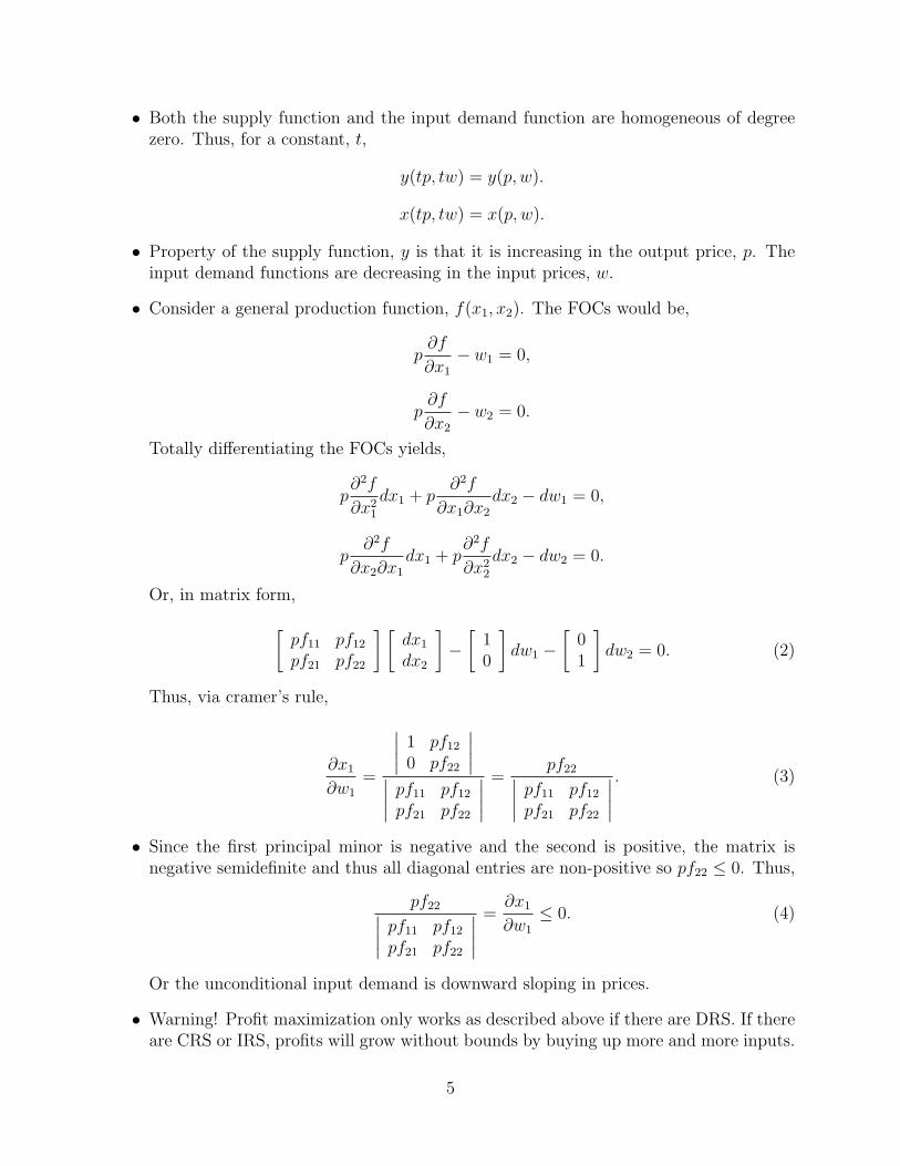
• Both the supply function and the input demand function are homogeneous of degreezero. Thus, for a constant, t,

y(tp, tw) = y(p, w).

x(tp, tw) = x(p, w).

• Property of the supply function, y is that it is increasing in the output price, p. Theinput demand functions are decreasing in the input prices, w.

• Consider a general production function, f(x1, x2). The FOCs would be,

p∂f

∂x1

− w1 = 0,

p∂f

∂x2

− w2 = 0.

Totally differentiating the FOCs yields,

p∂2f

∂x21

dx1 + p∂2f

∂x1∂x2

dx2 − dw1 = 0,

p∂2f

∂x2∂x1

dx1 + p∂2f

∂x22

dx2 − dw2 = 0.

Or, in matrix form,[pf11 pf12

pf21 pf22

] [dx1

dx2

]−[

10

]dw1 −

[01

]dw2 = 0. (2)

Thus, via cramer’s rule,

∂x1

∂w1

=

∣∣∣∣ 1 pf12

0 pf22

∣∣∣∣∣∣∣∣ pf11 pf12

pf21 pf22

∣∣∣∣ =pf22∣∣∣∣ pf11 pf12

pf21 pf22

∣∣∣∣ . (3)

• Since the first principal minor is negative and the second is positive, the matrix isnegative semidefinite and thus all diagonal entries are non-positive so pf22 ≤ 0. Thus,

pf22∣∣∣∣ pf11 pf12

pf21 pf22

∣∣∣∣ =∂x1

∂w1

≤ 0. (4)

Or the unconditional input demand is downward sloping in prices.

• Warning! Profit maximization only works as described above if there are DRS. If thereare CRS or IRS, profits will grow without bounds by buying up more and more inputs.

5

2.1 Properties of the Profit Function

• π(p, w) is non-decreasing in p and is non-increasing in wi for i = 1...n.Proof: Let p′ > p. Thus,

π(p, w) ≤ p′y(p, w)− wx(p, w) ≤ π(p′, w)

This first inequality is just algebra, but the second comes from the fact that π ismaximized for (p′, w) so using any other (p∗, w∗) will yield lower profits.Thus if p′ > p, Then π(p′w) ≥ π(p, w), or π(p, w) is non-decreasing in p.

• π(p, w) is homogeneous of degree 1 in prices. Proof: By definition,

py(p, w)− wx(p, w) ≥ py′ − wx′ ∀ (y′,−x′) ∈ Y,

because the first expression of profits is evaluated at the profit maximizing values of pand w. Multiplying both sides by t,

tpy(p, w)− twx(p, w) ≥ tpy′ − twx′ ∀ (y′,−x′) ∈ Y

Hence, (y(p, w),−x(p, w)) is the production plan that maximizes profits at (tp, tw).Thus π(tp, tw) = tπ(p, w), or π is homogeneous of degree 1.

• π(p, w) is convex in prices.Proof: Take prices (p, w) and (p′, w′) and define,

(p′′, w′′) = λ(p, w) + (1− λ)(p′, w′) for λ ∈ [0, 1].

Now, by definition of profit maximization,

py(p′′, w′′)− wx(p′′, w′′) ≤ π(p, w).

Mulitplying both sides by λ, (∗)

λpy(p′′, w′′)− λwx(p′′, w′′) ≤ λπ(p, w).

Also by definition of profit maximization,

p′y(p′′, w′′)− w′x(p′′, w′′) ≤ π(p′, w′).

Mulitplying both sides by (1− λ), (∗∗)

(1− λ)p′y(p′′, w′′)− (1− λ)w′x(p′′, w′′) ≤ (1− λ)π(p′, w′).

Summing (∗) and (∗∗), yields,

p′′y(p′′, w′′)− w′′x(p′′, w′′) ≤ λπ(p, w) + (1− λ)π(p′, w′).

Thus,π(p′′, w′′) ≤ λπ(p, w) + (1− λ)π(p′, w′).

So, π is convex. QED.

• π(p, w) is continuous on (p, w).Proof: QED.

6

3 Week 3

3.1 Duality

• We have shown thus far that f(x) −→ y(p, w), x(p, w) −→ π(p, w).

• But can we go the other direction? yes. To do this, we first need the envelope theorem.

• Envelope Theorem: Supose that we maximize a function g(s, a) with respect to s wherea is a parameter. We would obtain a solution s(a). Now define the maximized valueof the function as M(a) = g(s(a), a). By the chain rule,

dM(a)

da=

∂g

∂s

∂s

∂a+

∂g

∂a.

But since we already defined s(a) to be the maximium solution of g,∂g

∂s= 0. Thus

dM(a)

da=

∂g

∂a.

• Now consider the profit function,

π(p, w) = py(p, w)− wx(p, w).

Thus, by the envelope theorem,

∂π

∂p= y(p, w).

∂π

∂wi

= −xi(p, w).

Thus,∂2π

∂p2=

∂y(p, w)

∂p≡ Slope of the Supply Function.

The slope of the supply function is positive because π is convex. Also,

∂2π

∂w2i

= −∂xi(p, wi)

∂wi

≥ 0.

Thus, the input demands are downward sloping. Finally,

∂2π

∂wi∂wj

= −∂xi(p, w)

∂wi

= −∂xi(p, w)

∂wj

=∂2π

∂wj∂wi

.

Because the order that you take the partials does not matter (Young’s Theorem).

• This process of taking the partials of the profit function with respect to price, p, to findthe supply function, and with respect to the input price, w, to find the input demandis called the Hotelling Lemma.

7

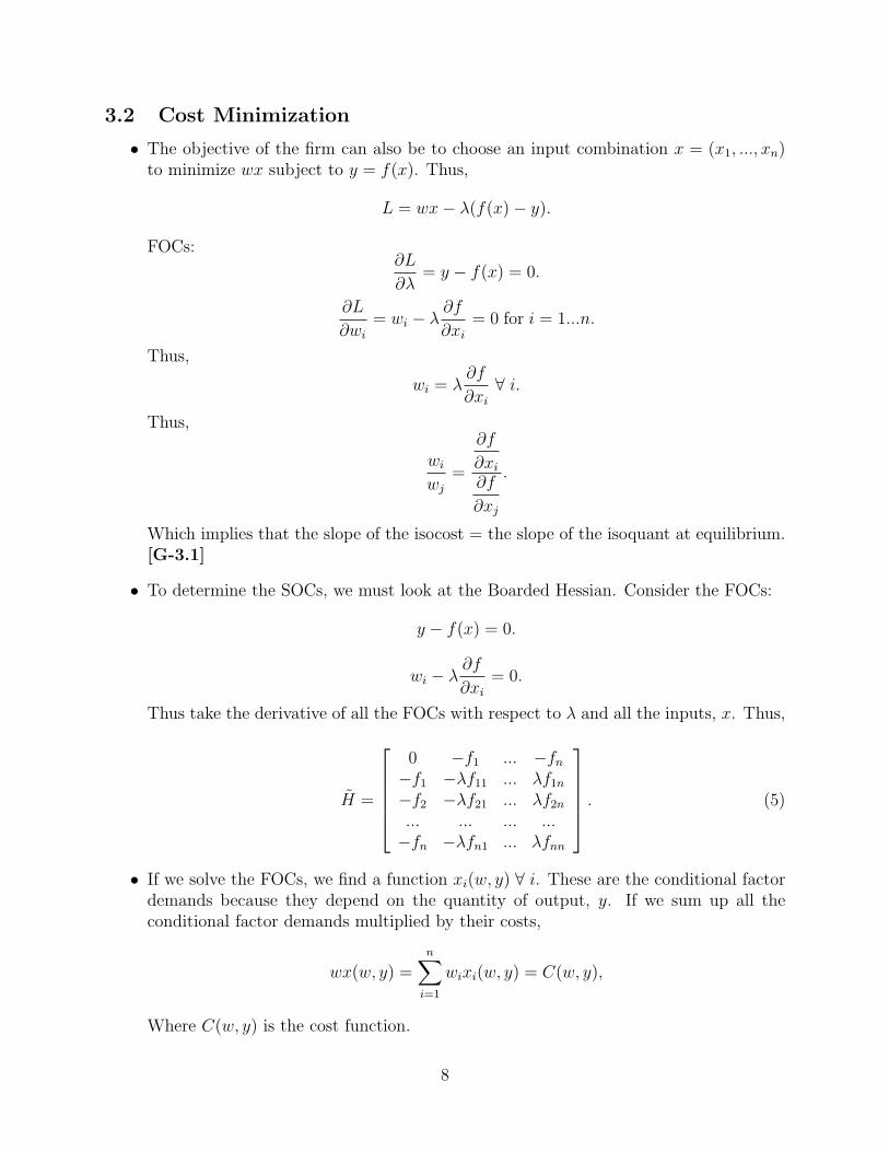
3.2 Cost Minimization

• The objective of the firm can also be to choose an input combination x = (x1, ..., xn)to minimize wx subject to y = f(x). Thus,

L = wx− λ(f(x)− y).

FOCs:∂L

∂λ= y − f(x) = 0.

∂L

∂wi

= wi − λ∂f

∂xi

= 0 for i = 1...n.

Thus,

wi = λ∂f

∂xi

∀ i.

Thus,

wi

wj

=

∂f

∂xi

∂f

∂xj

.

Which implies that the slope of the isocost = the slope of the isoquant at equilibrium.[G-3.1]

• To determine the SOCs, we must look at the Boarded Hessian. Consider the FOCs:

y − f(x) = 0.

wi − λ∂f

∂xi

= 0.

Thus take the derivative of all the FOCs with respect to λ and all the inputs, x. Thus,

H =

0 −f1 ... −fn

−f1 −λf11 ... λf1n

−f2 −λf21 ... λf2n

... ... ... ...−fn −λfn1 ... λfnn

. (5)

• If we solve the FOCs, we find a function xi(w, y) ∀ i. These are the conditional factordemands because they depend on the quantity of output, y. If we sum up all theconditional factor demands multiplied by their costs,

wx(w, y) =n∑

i=1

wixi(w, y) = C(w, y),

Where C(w, y) is the cost function.

8

• Properties of the Cost Function, C(w, y).

– C(w, y) is nondecreasing in wi for i = 1...n.

– C(w, y) is homogeneous of degree 1 in w.

– C(w, y) is concave in w.

– C(w, y) is continuous in w.

• Duality of the Cost Function:

C(w, y) =n∑

i=1

wixi(w, y).

Thus, by the envelope theorem,

∂C(w, y)

∂wi

= xi(w, y) ∀ i.

So by the Shephard’s Lemma, taking the partial of the cost function with respect tothe input prices yields the respective input demand function. Also,

∂2C(w, y)

∂w2i

=∂xi(w, y)

∂wi

≡ Slope of the Conditional Factor Demand.

Since the Cost function is concave, C is negative semidefinite. Thus all diagonal entriesare negative. Thus the conditional input demand functions are downward sloping.

• Finally, having obtained now the cost function, we can write it simply as C(y). Thus,

π = py − C(y).

To maximize profits, a firm chooses y to maximize py − C(y), thus the FOC:

∂π

∂y⇒ p− ∂C

∂y= 0.

Or the familiar result,Price = Marginal Cost.

9

4 Week 4

• Costs: C(y) = V C(y)+F , where V C are the variable costs that depend on the quantityof output and F are the fixed costs. Fixed costs can be divided into Long and Shortrun fixed costs.

• Average Costs:

AC(y) =V C(y)

y+

F

y= AV C(y) + AFC(y).

• If AC(y) is decreasing in y, then we have economies of scale.

• If AC(y) is increasing in y, then we have diseconomies of scale.

• IRS ⇒ Economies of Scale, but NOT necessarily vice versa. Symmetrically, DRS ⇒Diseconomies of Scale but NOT vice versa.

• Marginal Cost:dC(y)

dy= C ′(y) ≡ MC.

• Since AC(y) =C(y)

y,

AC ′(y) =d

dy

[C(y)

y

]=

yC ′(y)− C(y)

y2=

C ′(y)

y− C(y)

y2.

Therefore, when AC ′(y) = 0,C ′(y)

y=

C(y)

y2.

C ′(y) = MC(y) =C(y)

y.

Or the MC intersects the AC curve at the minimum of the AC. The same can beshown for the AV C : MC = AV C at the minimum of the AV C.

• Short Run Firm Supply.

– Assume fixed costs are sunk. Thus,

πSR = y(P − AV C(y))− F.

Firms only supply product if P > AV C(y), so graphically [G-4.1] the shortrun supply curve is the MC curve above the minimum of the AV C curve and 0elsewhere.

– Short run aggregate supply assuming m firms:

Y (p) =m∑

i=1

yi(p).

10

• Long Run Firm Supply.

– A firm’s supply is positive if p > min(AC).

– Assume no barriers to entry.

– Thus if p > min(AC), π > 0 and firms have an incentive to enter and drive theprice down.

– Also if p < min(AC), π < 0 and firms have an incentive to exit and bring up theprice.

– Thus, in equilibrium, p = min(AC), or the long run supply curve is perfectlyelastic.

• More on Duality. We have shown that via shepherd’s lemma, we can go from thecost function to the conditional factor demands by differentiating C(y) with respectto w. But can we go from the conditional factor demands to the technology? Yes, inmost cases. By looking at several input and price combinations and determining theequilibrium we begin to trace out an isoquant by looking at the slope of the isocostlines at each point. This only works if the technology is convex! [G-4.2]

4.1 Consumer Theory

• Consumer chooses best (based on preferences) available (based on budget constraint)choice.

• Domain of choice: the consumption set, X ⊆ Rn+. A typical element of X is x =

(x1, ..., xn), which is a consumption bundle.

• Preferences:

– x �p y ≡ “x is weakly prefered to y.”

– x �p y ≡ “x is strictly prefered to y if x �p y but NOT y �p x.”

– x ∼p y ≡ “x is indifferent to y if x �p y and y �p x.”

– Properties of Preferences.

∗ Completeness: For any x, y ∈ X, either x �p y or y �p x, or both. Thus allbundles can be ranked.

∗ Transitivity: For x, y, z ∈ X, if x �p y and y �p z, then x �p z. Also holdsfor strict preference and indifference.

• Theorem: Suppose the consumption set, X, is finite. If preferences are complete andtransitive, then there exists a function u : X 7→ R 3 ∀ x, y ∈ X, u(x) ≥ u(y) if andonly if x �p y.Proof: Suppose, for simplicity, all bundles are ordered by strict preference. Then thereexists a most preferred bundle. To show this, proceed by contradiction. Assume thereis not a most preferred bundle. Then for any bundle, say x′, I can find another bundle,

11

x′′, such that x′′ �p x′. Starting with x′′, there exists a x′′′ such that x′′′ �p x′′. And soon... If there is only a finite number of bundles some bundles must be repeated. Butthis contradicts transitivity. So there must exist a most preferred bundle, call it x∗.Set u(x∗) = c1, where c1 is a constant. Now find the second most prefered bundle, y∗

and set u(y∗) = c2 where c2 < c1. This can continue until u(·) is completely defined asdescribed above. QED.

4.2 More Accurate Definiteness Properties

• Test for definiteness as it applies to symmetric matrices (such as the Hessian):

• The matrix is positive definite iff all the leading principal minors are strictly positive.

• The matrix is negative definite iff all the odd-order leading principal minors are strictlynegative and all the even-order leading principal minors are strictly positive.

• The matrix is positive semidefinite iff every principal minor (leading and nonleading)is nonnegative.

• The matrix is negative semidefinite iff every principal minor (leading and nonleading)of odd-order is not positive, and every principal minor of even-order is not negative.

• Of course, if we find a matrix to be postive definite then we know it is positive semidef-inite and if we find matrix to be negative definite then it is negative semidefinite andwe therefore do not need to look at the nonleading principal minors.

• As an example, consider a 3x3 symmetric matrix where H1, H2, and H3 are the leadingprincipal minors:

If H1 > 0, H2 > 0, H3 > 0,

then the matrix is Postive Definite.

If H1 < 0, H2 > 0, H3 < 0,

then the matrix is Negative Definite.

If H1 > 0, H2 > 0, H3 = 0,

then the matrix is not definite.

In this case the matrix is either Postive Semidefinite or Indefinite. To determine ifit is positive semidefinite, we must test the rest of the principal minors (i.e. thenon-leading ones). If every principal minor is nonnegative, then the matrix is indeedpositive semidefinite.

If H1 < 0, H2 > 0, H3 = 0,

12

then the matrix is either Negative Semidefinite or Indefinite.

Again, we must test all the principal minors to determine if it is negative semidefinite.

If H1 = 0, H2 > 0, H3 = 0,

then the matrix is either Postitive Semidefinite,

Negative Semidefinite, or Indefinite.

Again, we must test all principal minors to determine which it is.

• NOTE: When considering a Boardered Hessian, everything is the exact opposite. Youget negative semi-definitness when the odd principal leading minor determinants areall non-negative and the even are non-positive. This excludes the first, which is alwayzero, and the second which is always negative, so you only have to worry about the3rd and greater. For a negative definite hessian matrix therefore, all principal minordeterminants must be strictly positive!

13

5 Week 5

• Utility is an ordinal concept. Only the relative ranks matter. If u(x) represents thepreferences of the consumer, so does u(x) + c because all utility levels just shift by cbut the relative position remains the same.

• Any monotonic transformation that preserves the intial utility ranking leaves the utilityfunction unchanged. Thus [u(x)]k and ln(u(x)) are ok transformations.

• Definition: Utility function.

u : x 7−→ R 3 x �p y iff u(x) ≥ u(y) for any x, y ∈ X.

• Utility functions are transitive and complete.

• Definition: Indifference Curves: The set of consumption bundles, x, for which u(x) isconstant.

• Consider the case of two commodities so that x = (x1, x2). An indifference curve isthen u(x1, x2) = c, where c is constant. Totally differentiating,

∂u

∂x1

dx1 +∂u

∂x2

dx2 = 0.

Thus,

dx2

dx1

=∂u∂x1

∂u∂x2

.

Or,dx2

dx1

= The slope of the indifference curve.

Thus the slope of the indifference curve equals the Marginal Rate of Substitution(MRS).

• Example: Cobb-Douglas Utility function. u(x1, x2) = xα1 xβ

2 . Thus,

MRS =αxα−1

1 xβ2

βxα1 xβ−1

2

=αx2

βx1

.

• Example: Perfectly Substitutable Commodities: u(x1, x2) = ax1 + bx2. Thus,

MRS =a

b.

• Example: Perfectly Complementary Commodities: u(x1, x2) = min{ax1, bx2}. Thus,

MRS = Undefined.

This is because the indifference curves are rectangular so we get a corner solution wherethe slope is undefined.

14

5.1 The Consumer’s Problem

• A consumer chooses a consumption bundle x = (x1, x2, ..., xn) to maximize u(x1, x2, ..., xn)subject to p1x1 + p2x2 + ... + pnxn ≤ m, where m is the consumer’s income.

• Notice that the constraint is written as an inequality. It can be written as a strictequality if we have the following assumption.

• Local NonSatiation (LNS)

For any x ∈ X and ε > 0,∃ y ∈ X 3 d(x, y) < ε and u(y) > u(x).

Where d(x, y) represents the distance between x and y. So in words, it just means thatfor any bundle of goods, we can find some other bundle close to it where the utilityat the new bundle is strictly greater. A little more (possibly very little) can always bebetter.

• If utility functions are monotonic, you definitely get LNS, but not vice versa. HavingLNS does not necessarily mean that u(x) is monotonic. Monotonicity is stronger thanLNS.

• If LNS holds, you cannot be in an equilibrium state where you are not spending allavailable income. You can spend a little bit more and make yourself strictly betteroff. Thus, repeating this process, you eventually reach your income so the consumer’sproblem changes.

• Consumer’s Problem assuming LNS. Choose x ∈ X to maximize,

u(x1, x2, ..., xn),

subject to,p1x1 + p2x2 + ... + pnxn = m.

Or in vector notation, maximize:

u(x) subject to px = m,

where p is a price vector.

• Solving the Consumer’s Problem, via the LaGrangian,

L = u(x) + λ(m− px).

• FOCs:∂L

∂λ= m− px = 0.

∂L

∂xi

=∂u

∂xi

− λpi = 0 ∀ i.

15

• SOCs. Let the first FOC be L1 and the second set of FOCs be L2, L3, · · · .

H =

∂L1

∂λ

∂L1

∂x1

...∂L1

∂xn∂L2

∂λ

∂L2

∂x1

...∂L2

∂xn∂L3

∂λ

∂L3

∂x1

...∂L3

∂xn

... ... ... ...∂Ln

∂λ

∂Ln

∂x1

...∂Ln

∂xn

=

0 −p1 ... −pn

−p1 u11 ... u1n

−p2 u21 ... u2n

... ... ... ...−pn un1 ... unn

. (6)

• This boardered Hessian matrix, H, should be negative semidefinite because we arelooking for a maximum. Thus the leading principal minor determinants starting withthe 3rd should alternate in sign and the 3rd should be positive. Note again that thisapplies only to boardered hessians because we are adding on an extra row and columnso everything is backward compared a regular matrix. Note that you start with the3rd because the 1st is always 0 and the 2nd is always negative.

• Now consider the second set of FOCs:

∂L

∂xi

=∂u

∂xi

− λpi = 0 ∀ i.

Thus,∂u

∂xi

= λpi.

Therefore comparing commodity i and j, we have

∂u∂xi

∂u∂xj

=pi

pj

.

Which in words says that the Marginal Rate of Substitution (MRS) is equal to theprice ratio, which is the slope of the Budget Constraint (BC).

• In order to have one unique solution to the consumer’s problem, there must exist onlyone tangency between the consumer’s indifference curves and budget constraint. Thus,Convex indifference curves or therefore Quasi-concave utility functions will avoid anyproblems with multiple solutions. [G-5.1]

• Example using Cobb-Douglas Utility Function: u(x1, x2) = xα1 xβ

2 . Thus,

MRS =αx2

βx1

=p1

p2

.

p2x2 =β

αp1x1.

16

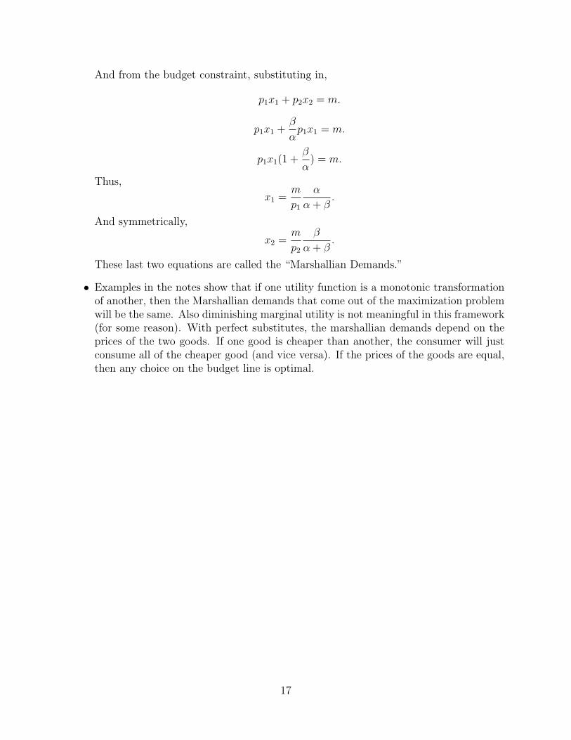
And from the budget constraint, substituting in,

p1x1 + p2x2 = m.

p1x1 +β

αp1x1 = m.

p1x1(1 +β

α) = m.

Thus,

x1 =m

p1

α

α + β.

And symmetrically,

x2 =m

p2

β

α + β.

These last two equations are called the “Marshallian Demands.”

• Examples in the notes show that if one utility function is a monotonic transformationof another, then the Marshallian demands that come out of the maximization problemwill be the same. Also diminishing marginal utility is not meaningful in this framework(for some reason). With perfect substitutes, the marshallian demands depend on theprices of the two goods. If one good is cheaper than another, the consumer will justconsume all of the cheaper good (and vice versa). If the prices of the goods are equal,then any choice on the budget line is optimal.

17

6 Week 6

• Perfect Complements Utility Functions: u(x1, x2) = min{ax1, bx2}. Let a = b = 1 andwe know that because of the rectangular utility functions [G-6.1], the optimal solutionwill be such that x1 = x2. Thus the budget constraint becomes,

p1x1 + p2x2 = p1x1 + p2x1 = m.

Thus, the marhshallian demands,

x1 =m

p1 + p2

.

x2 =m

p1 + p2

.

• Quasi Linear Utility Functions: u(x1, x2) = 2√

x1 + x2, where the first term is clearlynonlinear but the rest is linear. To solve this for the Marshallian demands, do theusual and set MRS = Price Ratio. Thus,

ux1

ux2

=p1

p2

⇒ x−1/21

1=

p1

p2

.

Thus,

x1 = (p2

p1

)2.

And substituting into the budget constraint,

p1(p2

p1

)2 + p2x2 = m ⇒ x2 =m

p2

− p2

p1

.

The only problem with this is x2 might be negative under the right choices for m, p1,and p2. Thus Marshallian demands are,

x1 = (p2

p1

)2 and x2 =m

p2

− p2

p1

ifm

p2

− p2

p1

≥ 0.

x1 =m

p1

and x2 = 0 ifm

p2

− p2

p1

< 0.

Thus with quasi-linear utility functions, one must be careful because the tangencycondition might yield negative demands and thus the solution needs to be adjusted toreflect this. [G-6.2]

6.1 Price and “and” Income Changes

• Price Offer Curve: Take your typical utility maximizing setup with the utility curvejust tangent to the budget constraint. Then change the price of one of the commodities.Thus the budget line shifts and you will get a new equilibrium at a new utility level.Continuing this process and connecting the equilibrium points yields the Price OfferCurve. If the curve slopes downward in xi, pi space then the good is called Ordinary:The lower the price of good i, the more of it that is demanded.

18

• If the price offer curve slopes upward in xi, pi space then the good is called a GiffenGood: The lower the price of good i, the less of it that is demanded. [G-6.3]

• Now consider the same utility/budget constraint set up and vary the income level.Record the different equilibriums as you adjust income. The curve that connects allthe equilibriums is called the Income Expansion Path. Drawn in xi, m space it isrefered to as an Engel Curve. If the Engel curve slopes upwards in xi, m space, thenthe good is called a Normal Good: The higher a consumer’s income level, the more ofgood i that is demanded.

• If the Engel curve slopes downwards in xi, m space, then the good is called an InferiorGood: The higher a consumer’s income level, the less of good i that is demanded.Examples of inferior goods are cheap food products and even cigarettes. [G-6.4]

6.2 Indirect Utility Functions

• From Utility maximization, we obtain a vector of marshallian demands x(p, m). Plug-ging the vector of marshallian demands into the utility function, we obtain the IndirectUtility Function, v(p, m). That is,

v(p, m) = u(x(p, m)).

• Example of a Cobb Douglas Utility Function: u(x1, x2) = x1x2. MRS = Price ratioimplies,

∂u∂x1

∂u∂x2

=p1

p2

⇒ x2

x1

=p1

p2

.

Thus,

x1 = x2(p2

p1

).

x2 = x1(p1

p2

).

And substituting into the budget constraint,

m = p1x1 + p2[x1(p1

p2

)] = 2p1x1.

So Marshallian Demands,

x1 =m

2p1

.

x2 =m

2p2

.

Substituting the Marshallian demands back into the utility functions,

v(p, m) = u(x1(p1, m), x2(p2, m)) =m

2p1

m

2p2

=m2

4p1p2

.

19

6.3 Properties of the Indirect Utility Function

• Non-increasing in p and non-decreasing in m. See notes for simple proof.

• Homogeneous of degree 0 in (p, m). If all prices and income level go up by the sameamount, the budget line doesn’t shift at all, thus the utility level is constant. tpx =tm ⇒ px = m.

• Quasi-Convex in Prices.Proof: Take two prices vectors, p and p′ and consider another price vector,

p′′ = λp + (1− λ)p′ with λ ∈ [0, 1].

Now consider a consumption bundle, x∗ 3 p′′x∗ ≤ m. Thus x∗ is affordable at prices,p′′. This implies that x∗ must be affordable at either p, p′, or both. Thus px∗ ≤ m orp′x∗ ≤ m or both. Hence,

v(p′′, m) ≤ max{v(p, m), v(p′, m)}.

Which is the definition of quasi-convex in p.

• v(p, m) is continuous if u(x) is continuous. No proof.

6.4 Expenditure Function

• A consumer chooses the bundle x to minimize px subject to u(x) ≥ u. As a sim-ply analogue to the cost function of the firm, out of this optimisation we obtain anexpenditure function with the same properties as the cost function.

• Properties of the Expenditure function e(p, u): 1) Non-decreasing in p; 2) Homogeneousof degree 1 in p; 3) Concave in p; 4) Continuous.

• Just as we took the partial of the cost function with respect to input prices to getthe conditional factor demands (via Shephard’s lemma), we can take the partial ofthe expenditure function with respect to prices to get the compensated or HicksianDemands.

∂e(p, u)

∂pi

= hi(p, u).

• Next we have a series of identities which we will use in the coming sections,

Identity 1: e(p, v(p, m)) = m.

Identity 2: v(p, e(p, u)) = u.

Identity 3: hi(p, v(p, m)) = xi(p, m).

Identity 4: xi(p, e(p, u)) = hi(p, u).

20

• Taking the total differential of the 2nd identity,

∂v(p, e(p, u))

∂pi

+∂v(p, e(p, u))

∂m

∂e(p, u)

∂pi

= 0.

∂v(p, e(p, u))

∂pi

+∂v(p, e(p, u))

∂mhi(p, u) = 0.

Evalutated at u = v(p, m),

∂v(p, m)

∂pi

+∂v(p, m)

∂mxi(p, m) = 0.

Hence solving for the Marshallian demand,

xi(p, m) = −

∂v(p, m)

∂pi

∂v(p, m)

∂m

.

This last Equality is called Roy’s Identity named after Roy. You can obtain Marshalliandemands from the indirect utility function.

• Example of finding an expenditure functions: Consider a Cobb Douglas Utility func-tion: u = x1x2. Thus,

v(p, m) =1

4

m2

p1p2

.

Solving for m,m = 2

√p1p2v(p, m) = 2

√p1p2u = e(p, u).

• We would now like to develop restrictions on the Marshallian demands. Consider,

Identity 4: xi(p, e(p, u)) = hi(p, u).

• Taking to total differential,

∂xi(p, e(p, u))

∂pj

+∂xi(p, e(p, u))

∂m

∂e(p, u)

∂pj

=∂hi(p, u)

∂pj

.

∂xi(p, e(p, u))

∂pj

+∂xi(p, e(p, u))

∂mhj(p, u) =

∂hi(p, u)

∂pj

.

Evluated at u = v(p, m),

∂xi(p, m)

∂pj

+∂xi(p, m)

∂mxj(p, m) =

∂hi(p, u)

∂pj

.

And this last equality is called the Slutsky Equation. Note that the left side onlydepends on p and m which are usually observable quantities.

21

• Simplfying the notation of the Slutsky equation,

∆ij(p, m) =∂hi(p, u)

∂pj

.

Thus in matrix form,

∆11 . . . ∆1n...

. . ....

∆n1 . . . ∆nn

=

h1

p1

. . .h1

pn...

. . ....

hn

p1

. . .hn

pn

. (7)

• Notice that the right hand matrix of partials of the hicksian demand equation is equiv-alent to the matrix of second partials of the expenditure function. Thus since e(p, u)is concave, this matrix must be negative semidefinite. Thus the left hand matrix mustalso be negative semidefinite. The ∆ij(p, m) matrix is called the Substitution Matrix.

• Finally, rearranging the terms of the Slutsky equation,

∂x1

∂p1

=∂h1

∂p1︸︷︷︸Substitution−Effect

− ∂x1

∂m︸︷︷︸Income−Effect

x1.

Since∂h1

∂p1

(the substitution effect) is always negative and∂x1

∂mis positive when x1 is a

normal good,∂x1

∂p1

< 0 or demand for good i is downward sloping as would be expected.

• If∂x1

∂m< 0 then we have an inferior good. If this income effect term is large enough

(negative enough), then∂x1

∂p1

might actually become positive which would imply that

the commodity is a giffen good. Thus ALL giffen goods are inferior but not vice versa.

22

7 Week 7

7.1 Comparative Statics

• The Consumer’s Problem: Choose x ∈ X to maximize u(x) subject to px = m. Set upthe lagrangian: L = u(x)+λ(m−px) which yields FOCs (for the case of 2 commodities),

∂L

∂λ= m− p1x1 − p2x2 = 0.

∂L

∂x1

=∂u

∂x1

− λp1 = 0.

∂L

∂x2

=∂u

∂x2

− λp2 = 0.

• Totally differentiating the first FOC for utility maximization yields,

dm− x1dp1 − p1dx1 − x2dp2 − p2dx2 = 0.

Or,−p1dx1 − p2dx2 = x1dp1 + x2dp2 − dm.

• The second FOC:u11dx1 + u12dx2 − λdp1 − p1dλ = 0.

Or,−p1dλ + u11dx1 + u12dx2 = λdp1.

• Similarly for the third FOC:

u22dx2 + u21dx1 − λdp2 − p2dλ = 0.

Or,−p2dλ + u21dx1 + u22dx2 = λdp2.

• Written in matrix form then, 0 −p1 −p2

−p1 u11 u12

−p2 u12 u22

dλdx1

dx2

=

x1

λ0

dp1 +

x2

0λ

dp2 +

−100

dm. (8)

• Via cramer’s rule on the above matrix, one can find all the effects of prices and incomeand consumption under utility maximization. It can also show the decomposition ofdx1

dp1

into income and substitution effects (Slutsky Equations).

23

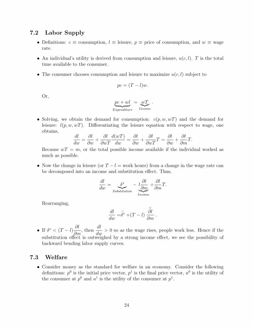
7.2 Labor Supply

• Definitions: c ≡ consumption, l ≡ leisure, p ≡ price of consumption, and w ≡ wagerate.

• An individual’s utility is derived from consumption and leisure, u(c, l). T is the totaltime available to the consumer.

• The consumer chooses consumption and leisure to maximize u(c, l) subject to

pc = (T − l)w.

Or,pc + wl︸ ︷︷ ︸

Expenditure

= wT︸︷︷︸Income

.

• Solving, we obtain the demand for consumption: c(p, w, wT ) and the demand forleisure: l(p, w, wT ). Differentiating the leisure equation with respect to wage, oneobtains,

dl

dw=

∂l

∂w+

∂l

∂wT

d(wT )

dw=

∂l

∂w+

∂l

∂wTT =

∂l

∂w+

∂l

∂mT.

Because wT = m, or the total possible income available if the individual worked asmuch as possible.

• Now the change in leisure (or T − l = work hours) from a change in the wage rate canbe decomposed into an income and substitution effect. Thus,

dl

dw= δs︸︷︷︸

Substitution

− l∂l

∂m︸︷︷︸Income

+∂l

∂mT.

Rearranging,

dl

dw=

−δs +(T − l)

+

∂l

∂m.

• If δs < (T − l)∂l

∂m, then

dl

dw> 0 so as the wage rises, people work less. Hence if the

substitution effect is outweighed by a strong income effect, we see the possibility ofbackward bending labor supply curves.

7.3 Welfare

• Consider money as the standard for welfare in an economy. Consider the followingdefinitions: p0 is the initial price vector, p1 is the final price vector, u0 is the utility ofthe consumer at p0 and u1 is the utility of the consumer at p1.

24

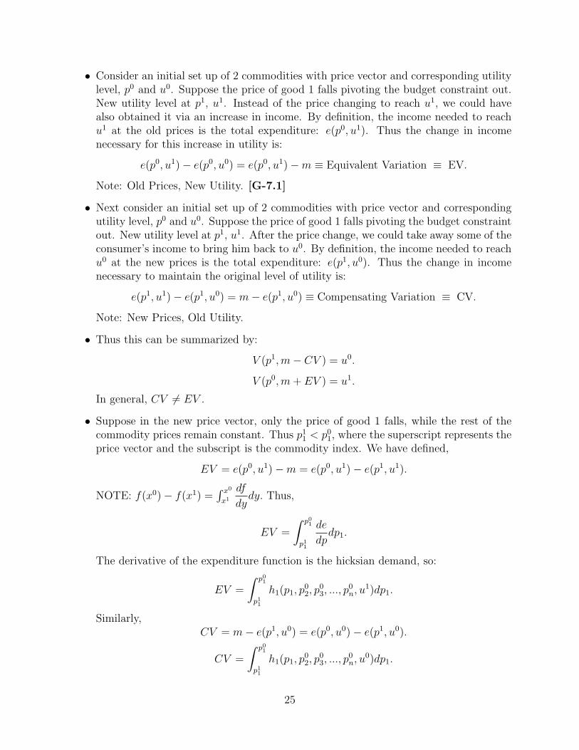
• Consider an initial set up of 2 commodities with price vector and corresponding utilitylevel, p0 and u0. Suppose the price of good 1 falls pivoting the budget constraint out.New utility level at p1, u1. Instead of the price changing to reach u1, we could havealso obtained it via an increase in income. By definition, the income needed to reachu1 at the old prices is the total expenditure: e(p0, u1). Thus the change in incomenecessary for this increase in utility is:

e(p0, u1)− e(p0, u0) = e(p0, u1)−m ≡ Equivalent Variation ≡ EV.

Note: Old Prices, New Utility. [G-7.1]

• Next consider an initial set up of 2 commodities with price vector and correspondingutility level, p0 and u0. Suppose the price of good 1 falls pivoting the budget constraintout. New utility level at p1, u1. After the price change, we could take away some of theconsumer’s income to bring him back to u0. By definition, the income needed to reachu0 at the new prices is the total expenditure: e(p1, u0). Thus the change in incomenecessary to maintain the original level of utility is:

e(p1, u1)− e(p1, u0) = m− e(p1, u0) ≡ Compensating Variation ≡ CV.

Note: New Prices, Old Utility.

• Thus this can be summarized by:

V (p1, m− CV ) = u0.

V (p0, m + EV ) = u1.

In general, CV 6= EV .

• Suppose in the new price vector, only the price of good 1 falls, while the rest of thecommodity prices remain constant. Thus p1

1 < p01, where the superscript represents the

price vector and the subscript is the commodity index. We have defined,

EV = e(p0, u1)−m = e(p0, u1)− e(p1, u1).

NOTE: f(x0)− f(x1) =∫ x0

x1

df

dydy. Thus,

EV =

∫ p01

p11

de

dpdp1.

The derivative of the expenditure function is the hicksian demand, so:

EV =

∫ p01

p11

h1(p1, p02, p

03, ..., p

0n, u

1)dp1.

Similarly,CV = m− e(p1, u0) = e(p0, u0)− e(p1, u0).

CV =

∫ p01

p11

h1(p1, p02, p

03, ..., p

0n, u

0)dp1.

25

• Note that the only difference in the CV and EV is the utility levels. If p1 falls, u1 > u0,but comparing EV and CV will depend on if x1 is normal or inferior.

• Consider the marshallian demand which by an identity,

x1(p, m) = h1(p, v(p, m)).

Since v(p, m) is increasing in m, if good 1 is a normal good,dx1

dm> 0. Thus

dh1

dv(p, m)>

0 ordh1

du> 0. Thus we have EV ≥ CV iff the good is normal.

• Since we have defined EV and CV in terms of integrals, they can be viewed graphicallyas areas under curves. Consider good 1 as a normal good. Thus,

h1(p1, p02, p

03, ..., p

0n, u

0) ≤ h1

(p1, p

02, p

03, ..., p

0n, V (p1, p

02, p

03, ..., p

0n, m)

)︸ ︷︷ ︸

Marshallian Demand for x1

≤ h1(p1, p02, p

03, ..., p

0n, u

1).

for p11 ≤ p1 ≤ p0

1.

• A graphical display of this can be seen in notes. [G-7.2] In general, CV ≤ ConsumerSurplus (CS) ≤ EV .

• If Marshallian does not depend on income, h1(p) = x1(p) or the above inequalitybecomes equality and CV = CS = EV .

• Example of Welfare comparison. Suppose there are K consumers. Let xji (p, m

j) be thedemand for good i by consumer j having income mj. Thus in aggregate,

Di =K∑

j=1

xji (p, m

j) ≡ Aggregate Demand.

• More specifically, letxj

i = αj(p) + β(p)mj.

Thus, in aggregate,

Di =K∑

j=1

αj(p) + β(p)K∑

j=1

mj.

• So demand for good i can be throught of as consumer j’s demand with aggregateincome

∑j mj. However, aggregate demands are “distribution independent” iff every

consumer j has an indirect utility function,

vj(p, mj) = aj(p) + b(p)mj.

(Or any monotonic tranformation there of.)

26

• This type of indirect utility function is called a “Gorman Form.” It is satisfied ifconsumers have identical homothetic preferences or quasilinear preferences (relativelystrict conditions).

• Now suppose that consumers do have indirect utilities of the Gorman Form. Thus theaggregate indirect utility is,

V (p, m) = a(p) + b(p) + m,

where a(p) =∑K

j=1 aj(p) and m =∑K

j=1 mj.

• Suppose V (p1, m) − V (p0, m) = c > 0. At the price level p1, the aggregate indirectutility function of this society is higher. So is society better off? Yes, but only if thereis a redistribution of income. Consider new income levels:

(m1, m2, ..., mK)

such that,

aj(p′) + b(p′)mj = aj(p0) + b(p0)mj +c

k.

The last term is the redistribution term of the utility surplus spread out equally overall consumers.

• Does this work? To see that it does, sum both sides across consumers,

V (p′,∑

j

mj) = V (p0,∑

j

mj) + c.

Hence,K∑

j=1

mj = m.

Moreover, at income levels, (m1, m2, ..., mK), every consumer is better off. Fascinating.

27

8 Week 8

8.1 Cost of Living Indices

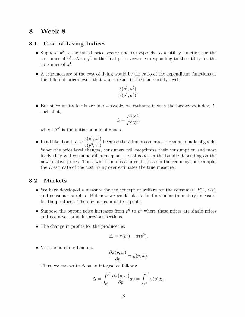
• Suppose p0 is the initial price vector and corresponds to a utility function for theconsumer of u0. Also, p1 is the final price vector corresponding to the utility for theconsumer of u1.

• A true measure of the cost of living would be the ratio of the expenditure functions atthe different prices levels that would result in the same utility level:

e(p1, u0)

e(p0, u0).

• But since utility levels are unobservable, we estimate it with the Laspeyres index, L,such that,

L =P 1X0

P 0X0,

where X0 is the initial bundle of goods.

• In all likelihood, L ≥ e(p1, u0)

e(p0, u0)because the L index compares the same bundle of goods.

When the price level changes, consumers will reoptimize their consumption and mostlikely they will consume different quantities of goods in the bundle depending on thenew relative prices. Thus, when there is a price decrease in the economy for example,the L estimate of the cost living over estimates the true measure.

8.2 Markets

• We have developed a measure for the concept of welfare for the consumer: EV , CV ,and consumer surplus. But now we would like to find a similar (monetary) measurefor the producer. The obvious candidate is profit.

• Suppose the output price increases from p0 to p1 where these prices are single pricesand not a vector as in previous sections.

• The change in profits for the producer is:

∆ = π(p1)− π(p0).

• Via the hotelling Lemma,∂π(p, w)

∂p= y(p, w).

Thus, we can write ∆ as an integral as follows:

∆ =

∫ p1

p0

∂π(p, w)

∂pdp =

∫ p1

p0

y(p)dp.

28

• Therefore, as seen in the notes [G-8.1], the difference in profits, ∆, or otherwise called“Producer Surplus,” can be shown as the different between the two prices under thesupply curve.

• The same graph can be drawn for aggregate supply with the area representing aggregateproducer surplus.

8.3 Price Formation

• Equilibrium market price is defined in elementary economics where Demand, D(p),equals Supply, S(p).

• To measure the responsiveness of these curves to prices, one could look at the slopes ofthe curves, but unfortunately because of a difference in units, two equilivalent demandor supply functions might have different slopes. Thus, consider elasticities:

Elasticity of Demand: εD =dD(p)

dp

p

D(p).

Elasticity of Supply: εS =dS(p)

dp

p

S(p).

8.4 Taxes

• Two types of taxes, quantity taxes and value taxes.

• Let pD be the price paid by the consumer and let pS be the price received by producers.

• A Quantity tax at rate t per unit would be of form:

pD = pS + t.

• A Value tax at a rate t would be of the form:

pD = pS(1 + t).

• Graphically it can be shown (See notes for graph [G-8.2]) that the tax revenue fromthe tax is less than the loss of consumer and produce surpluses together. Thus, taxesare distortionary and inefficient and result in a dead weight loss:

Dead Weight Loss = Consumer Surplus + Producer Surplus - Tax Revenue > 0.

29

8.5 General Equilibrium - Beyond Mock Exam

• Consider a pure exchange economy with NO production.

• Suppose there are n commodities and K consumers who wish to trade their endowmentsof goods.

• Each consumer J is described as hairy and ugly (Ed) with (uJ , wJ) where uJ is J ’sutility function and wJ is J ’s endowment such that,

wJ = (wJ1 , wJ

2 , . . . , wJn).

• Consider the following example which will be developed throughout the analysis.

– Suppose K = 2 and n = 2. Let w1 = (3, 1) and w2 = (1, 3). The utility

functions of the two consumers are cobb-douglas such that,

u1 = x11x

12,

and,

u2 = x21x

22.

Note that the superscripts are consumer indices and the subscripts are

commodity indices.

• An allocation, x = (x1, x2, . . . , xK) assigns a consumption bundle xJ = (xJ1 , xJ

2 , . . . , xJK)

to each consumer J = 1...K.

• An allocation, x = (x1, x2, . . . , xK) is feasible if:

K∑J=1

xJ ≤K∑

J=1

wj.

This just means that an allocation is feasible if the quantities consumed in the bundledo not exceed the total endowments of the goods.

– In our example, x1 = x2 = (2, 2) is a feasible allocation. Note that

allocations that add up to less than the total endowment are obviously

feasible as well even though it would result in having to destroy some

goods to reach that allocation.

8.6 Walrasian Equilibrium

• Walrasian equilibrium, or otherwise called competitive or normal equilibrium, is a pair(p, x) where,

p = (p1, . . . , pn)

is a price vector and,x = (x1, . . . , xK)

is an allocation such that,

30

– (1) x is feasible.

– (2) xJ maximizes uJ(xJ) such that pxJ ≤ pwJ .

• So the allocation is feasible in that the total allocation quantities do not exceed thetotal endowments. Also the allocation maximizes the consumer utility such that at thecurrent price level, each consumer’s bundle is affordable for him.

• Back to our example.

– The Marshallian demands coming from the cobb-douglas utility functions

are:

x11 =

3p1 + p2

2p1

and x12 =

3p1 + p2

2p2

.

x21 =

p1 + 3p2

2p1

and x22 =

p1 + 3p2

2p2

.

– Looking at the individual market conditions (for each good):

Good 1:3p1 + p2

2p1

+p1 + 3p2

2p1

= 4.

Good 2:3p1 + p2

2p1

+p1 + 3p2

2p1

= 4.

– Solving the good 1 equation yields,

p1 = p2.

– Substituting this into the market for good 2 just tells us that the equation

is valid! We cannot actually solve for either prices but we do find

that the prices must be equal. Thus an equilibrium supports any set

of prices such that the two prices are equal.

– NOTE: Once we found the equilibrium in market 1, this automatically implied

equilibrium in market 2.

• Back in the general setting, consider the vector of demands for consumer J :

xJ(p, pwJ).

• xJ(p, pwJ) is homogeneous of degree 0 in prices because if you increase prices by t,you increase both income (via the endowments) and the price of goods the consumerpurchases. The net effect is 0. Thus, if p is an equilibrium price vector, so is tp. (Thuswe have a multiplicity of equilibrium price vectors.)

• Define a vector of excess demands, ZJ , as:

ZJ(p, pwJ) = xJ(p, pwJ)− wJ .

ZJ is how much more of each good in the bundle that consumer J wants beyondhis endowment. Clearly ZJ

i could be negative if a consumer would rather sell hisendowment than have more of good i.

31

• Assuming local non-satiation, the value of excess demand must be 0 because consumerschoose bundles on their budget constraint. Thus,

pZJ(p, pwJ) = 0.

• In the aggregate, define:

Z(p) =K∑

J=1

ZJ(p, pwJ),

as the aggregate excess demand over all consumers.

• Since pZJ(p, pwJ) = 0 for all J = 1...K consumers, then,

pZ(p) = 0.

• Thus Walras’ Law:

“The value of aggregate excess demand must be zero.”

Which in other words just means that aggregate expenditure equals aggregate income.

• Consider the following implication of Walras’ Law:

– Walras’ law says:

pZ(P ) = p1Z1(p) + p2Z2(p) + · · ·+ pnZn(p) = 0.

Suppose we have equilibrium in all but the nth market. Thus

piZi(p) = 0 ∀ i < n.

Thus, the last market must also be in equilibrium. So pnZn(p) = 0.

• NOTE: When we solve for competitive equilibrium prices, we set one price equal toone (ie p1 = 1) or define a numeraire. All other prices are measured in terms of thenumeraire.

8.7 Pareto Efficiency

• Consider K consumers. An allocation, x = (x1, . . . , xK) is pareto efficient if the fol-lowing is true:

– (1) x is feasible.

– (2) @ a different feasible allocation, x = (x1, . . . , xK) 3

uJ(xJ) ≥ uJ(xJ) ∀ J = 1...K,

and,uJ(xJ) > uJ(xJ) for some J.

• Thus all consumers cannot be at least as good off and at least one consumer cannotbe strictly better off.

32

9 Week 9

9.1 The First Theorem of Welfare

• Assume L.N.S. Then any competitive equilibrium allocation is pareto efficient.Proof: Consider a competitive equilibrium, (p, x). Proceed by contradiction. Supposex is not pareto efficient. There there exists a different feasible allocation x, such that,

(1) : uJ(xJ) ≥ uJ(xJ), J = 1...K.

(2) : uJ(xJ) > uJ(xJ), for at least one J.

By LNS, (1) implies, pxJ ≥ pwJ . If not, there would exist another bundle, xJ , thatwould make the consumer strictly better off: uJ(xJ) > uJ(xJ) ≥ uJ(xJ).Therefore, pxJ ≥ pwJ for J = 1...K. Hence (2) implies that at the equilibrium prices,the consumer cannot afford xJ(pxJ > pwJ). Then summing across consumers,

p

K∑J=1

xJ > pK∑

J=1

wJ .

Which contradicts feasibility. QED.

• Note that pareto efficiency does not imply desirability.

9.2 Is free trade a good thing?

• Suppose, utilities of consumers 1 and 2 with superscripts representing consumer indicesand the subscripts representing commodity indices:

u1 = x11x

12

andu2 = x2

1x22

with endowments:w1 = (3, 1)

andw2 = (1, 3).

• The equilibrium price would therefore be p1 = p2 = 1 and the equilibrium allocationwould be (2, 2) and (2, 2).

• Suppose now the utility of consumer 1 is:

u1 = x11x

12 − 2x2

1.

And for consumer 2:u2 = x2

1x22 − 2x1

2.

33

• Thus both consumers experience negative externalities from the other’s consumption.Plugging in the equilibrium values (2, 2),(2, 2) gives us u1 = u2 = 0. However, if tradeis not allowed and we consider the endowment utility level (3, 1), (1, 3), the utilitiesare u1 = u2 = 1. Thus the consumers are better off without trade! Thus a reason forregulation.

9.3 Edgeworth Box Analysis

• Refer to graphs in notes [G-9.1]. Under this setting the social planner’s problem is:Choose an allocation (x1, x2) to maximize,

u1(x1)

subject to:u2(x2)− u.

• The first order conditions are therefore tangency of each consumer’s indifference curvesto each other (and of course to their budget constraints.) Thus,

MRS1 = MRS2.

And,x1 + x2 = w1 + w2.

The second contraint is just the feasibility constraint.

• Note that this condition only holds for interior solutions.

• The set of Pareto efficient allocations is called the Contract Curve. [G-9.2]

• The Core is the area on the contract curve that makes both consumers better off (henceit is in “DEE LENZ.”)

• Since there are many pareto efficient equilibrium, which one is optimal? Thus thereis room for regulation, but not in setting consumption levels but rather in setting en-dowments and letting the market determine where people consume (Hence the SecondTheorem of Welfare).

• The FOC’s mentioned above for determining pareto efficient equilibria relies on thefact that preferences are convex.

9.4 Competitive Equilibrium with Production

• Consider 2 production processes that produce 2 commodities, y1 and y2 using the sameinput, x.

• Production process 1 is owned by agent A and is defined as:

y1 =√

x1.

34

• Production process 2 is owned by agent B and is defined as:

y2 =√

x2.

• The two agents, A and B, also have utility functions,

uA = yA1 yA

2 .

uB = yB1 yB

2 .

• Consider intial endowments,

wA = (y1, y2, x) = (0, 0, 5).

wB = (y1, y2, x) = (0, 0, 3).

• So the total amount of X available in the economy is 8 and note that the two agentsget no utility from possessing x so they would rather use it in production.

• Define P1 as the price of y1 and P2 as the price of y2. Let r be the price of x. Set anumeraire,

P2 = 1.

Thus the price ratio is defined as,

P =P1

P2

=P1

1= P1.

• As producers, both A and B maximize profits. Define profits:

πA = P1y1 − rx1 = P1

√x1 − rx1.

πB = P2y2 − rx2 = P2

√x2 − rx2.

• Thus first order conditions,

∂πA

∂x1

⇒ 1

2P1x

−1/21 − r =

1

2Px

−1/21 − r = 0.

∂πB

∂x2

⇒ 1

2P2x

−1/22 − r =

1

2x−1/22 − r = 0.

• Solving the FOC’s for x1:1

2Px

−1/21 − r = 0.

Px−1/21 = 2r.

x−1/21 =

2r

P.

x1/21 =

P

2r.

x1 =P 2

4r2.

35

• Solving the FOC’s for x2:1

2x−1/22 − r = 0.

x−1/22 = 2r.

x1/22 =

1

2r.

x2 =1

4r2.

• Substituting the input demand into the production function yields the supply of y1

and y2,

y1 =√

x1 =

√P 2

4r2=

P

2r.

y2 =√

x2 =

√1

4r2=

1

2r.

Therefore substituting into the profit functions,

πA = Py1 − rx1 = PP

2r− r

P 2

4r2=

2P 2

4r− P 2

4r=

P 2

4r.

πB = y2 − rx2 =1

2r− r

1

4r2=

2

4r− 1

4r=

1

4r.

• At the same time, both consumers maximize their utility. The income of each consumeris made up of their profits from making yi, and also what they get from selling thereendowment of x. Thus,

mA =P 2

4r+ 5r.

And,

mB =1

4r+ 3r.

• Because the utility functions are cobb-douglas, we can write the quantity demands ofyi as each consumer’s income level divided by two times the prices level. The demandfor commodity y1 for example:

yA1 =

P 2

4r+ 5r

2P.

yB1 =

1

4r+ 3r

2P.

Similiarly,

36

yA2 =

P 2

4r+ 5r

2.

yB2 =

1

4r+ 3r

2.

• Setting supply of y1 equal to the demand for y1,

P 2

4r+ 5r

2P+

1

4r+ 3r

2P=

P

2r.

1

2P

[P 2

4r+ 5r +

1

4r+ 3r

]=

P

2r.

P 2

2+ 10r2 +

1

2+ 6r2 = 2P 2.

P 2

2+ 16r2 +

1

2= 2P 2.

P 2 + 32r2 + 1 = 4P 2.

32r2 + 1 = 3P 2.

We also have the condition that the supply of x must add up to the total endowmentof x. Thus,

P 2

4r2+

1

4r2= 8.

Thus,P 2 + 1 = 32r2.

Substituting this into the equation above,

(P 2 + 1) + 1 = 3P 2.

P 2 + 2 = 3P 2.

2 = 2P 2.

P = 1.

Substituting this into the above equation to solve for r,

32r2 + 1 = 3(1).

32r2 = 2.

r2 =1

16⇒ r =

1

4.

37

Substituting in again to find the quantity of yA1 and yB

2 ,

yA1 =

P 2

4r+ 5r

2P=

1

1+ 5

4

2=

9

8.

yB1 =

1

4r+ 3r

2P=

1

1+ 3

4

2=

7

8.

• Setting supply of y2 equal to the demand for y2,

P 2

4r+ 5r

2+

1

4r+ 3r

2=

1

2r.

But we don’t need to solve this system because we used the numeraire so we can justplug in P and r to find the quantity of yA

2 and yB2 :

yA2 =

P 2

4r+ 5r

2=

1

1+

5

42

=9

8.

yB2 =

1

4r+ 3r

2==

1

1+

3

42

=7

8.

9.5 Two Production Processes - Marginal Rate of Transformation

• Consider two production processes: y1 = f1(x1) and y2 = f2(x2) where x1 + x2 = x.We can define a production possibilities frontier (see graph in notes [G-9.3]) such that,

y2 = T (y1).

• Thus, define the Marginal Rate of Transformation (MRT) as the slope of this curve:

dT (y1)

dy1

= −f ′2

f ′1

= −∂y2/∂x2

∂y1/∂x1

.

• The MRT is the trade off between y1 and y2 given that the input, x, is shared betweenthe two production processes.

38

10 Week 10

10.1 More on Pareto Efficiency

• With reference to the model from last week, we had two agents acting as both producersand consumers. We get pareto efficiency in the following way. Choose (yA

1 , yB1 , yA

2 , yB2 )

to maximize,uA(yA

1 , yA2 ),

subject to,uB(yB

1 , yB2 ) = u,

and,yA

2 + yB2 = T (yA

1 + yB1 ).

• So we maximize the one agents utility subject to the other attaining some fixed levelof utility. The second constraint just provides that we can get the full amount of y2 byapplying technology to y1.

• By varying u, we can find all possible pareto efficient points.

• Setting up the Lagrangian of the maximation above, yeilds FOCs. Solving the FOC’syields,

MRSA = MRSB = MRT.

10.2 Decision Under Uncertainty

• Let C be the set of N possible outcomes.

• A simply lottery, L, is a probability distribution, (P1, . . . , PN) over C, where Pi is theprobability of outcome i.

• Example C = (0, 100) and L = (12, 1

2) is like a simple coin toss lottery with equal

probability of winning 0 or 100.

• A Compound Lottery is (α1, . . . , αK , L1, . . . , LK) where αJ is the probability of lotteryLJ . From this compound lottery, we get a simple lottery, (P1, . . . , PN) where,

Pi =K∑

J=1

αJP Ji ,

where P Ji is the probability of outcome i in lottery J .

• Example of a Compound Lottery. Let C = (0, 100), L1 = (12, 1

2), and L2 = (0, 1).

Thus the compound lottery is (12, 1

2, L1, L2). The outcomes are still 0 and 100. But

now consider the probabilities of each of these outcomes. They are simply equal to

39

the probability of being in each lottery times the probability of attaining the outcome.Thus,

Prob(0) = α1P 11 + α2P 2

1 =1

2∗ 1

2+

1

2∗ 0 =

1

4.

P rob(100) = α1P 12 + α2P 2

2 =1

2∗ 1

2+

1

2∗ 1 =

3

4.

Thus the simple lottery becomes (14, 3

4).

10.3 Preference Properties Involving Lotteries

• Let L be the set of simple lotteries and let �P represent preferences of L. We haveseveral assumptions about �P .

• Assumption 1: �P is complete and transitive.

• Assumption 2: Continuity. For any 3 simple lotteries, L, L′, and L′′ ∈ L, the sets,{L ∈ [0, 1] 3 αL + (1− α)L′ �P L′′

}

and, {L ∈ [0, 1] 3 L′′ �P αL + (1− α)L′

}are closed sets. This is just a technical assumption. It says we have no jumps inpreferences.

• Assumption 3: Independence Axiom. For an 3 lotteries, L, L′, and L′′, and α ∈ [0, 1],then,

L �P L′ if and only if αL + (1− α)L′′ �P αL′ + (1− α)L′′.

Note that L′′ appears on both sides, so we really shouldn’t take it into account whendetermining our preferences between L and L′.

• Note that the independence axiom assumes the independence of the outcomes, butclearly in this case, you wouldn’t want to read about Paris knowing that you weren’tever going to get to go. People have regrets. But I still think this was a poor example.

• Now assuming that the assumptions and axioms above hold, then there exists a vectorof utilities (u1, . . . , uN) 3 for any 2 lotteries, L = (P1, . . . , PN) and L′ = (P ′

1, . . . , P′N),

L �P L′ if and only if EU(L) ≥ EU(L′).

L �P L′ if and only ifN∑

i=1

Piui ≥N∑

i=1

P ′iui.

Where EU(·) is the expected utility of the lottery.

40

• Note that if (u1, . . . , uN) represents the same preferences as (u1, . . . , uN), then it mustbe the case that,

ui = βui + γ,

with β > 0 and γ a constant. Note that just having a monotonic transformation of autility function is not enough (not strong enough). The transformation must be linearand increasing to maintain the preference relationships.

• Consider the importance of the Independence axiom with the following example. LetC = (C1, C2, C3), L = (1, 0, 0), L′ = (0, 1, 0), and L′′ = (0, 0, 1). Thus,

αL + (1− α)L′′ has utility: αu1 + (1− α)u3.

αL′ + (1− α)L′′ has utility: αu2 + (1− α)u3.

Now suppose,L �P L′.

Therefore by the independence axiom,

αL + (1− α)L′′ �P αL′ + (1− α)L′′.

Thus from above,αu1 + (1− α)u3 ≥ αu2 + (1− α)u3.

Simplifying,

u1 ≥ u2.

Fascinating.

10.4 Risk Preferences

• Now consider outcomes as “wealth” or “consumption.” A lottery in this case is acummulative distribution function, F (x) where F (x) = Prob(“wealth” ≤ x).

• The utility of F (x) is: ∫u(x)dF (x).

• If f(x) is the density of F , the utility is then,∫u(x)f(x)dx.

Which is the definition of expected utility as each level of utility, u(x), is weightedby its probability, f(x). In this case u(x) is called a “Bernoulli” or “Von Neumann -Morganstern” (VNM) utility function.

41

• 3 cases.

– For any lottery, F (x), then

u

(∫xdF (x)

)≥∫

u(x)dF (x)

implies Risk Aversion and Concave Utility Functions.

– For any lottery, F (x), then

u

(∫xdF (x)

)=

∫u(x)dF (x)

implies Risk Neutrality and Linear Utility Functions.

– For any lottery, F (x), then

u

(∫xdF (x)

)≤∫

u(x)dF (x)

implies Risk Lovingness and Convex Utility Functions.

10.5 Example of the Demand for Insurance

• Let M = initial wealth. L = Possible Loss. P = Probability of Loss. S = Amount ofInsurance Coverage. r = unit premium or price of insurance.

• Suppose the consumer buys S units of insurance. Then the lottery is as follows: Withprobability (1− P ), the consumer does not experience a loss and has payoff M − rS.With probablity, P , the consumer has the loss and has payoff M − L − rS + S =M − L + (1− r)S.

• The consumer chooses S to maximize,

(1− p)u

[M − rS

]+ pu

[M − L + (1− r)S

].

Yields FOC(S):

−(1− p)ru′(M − rS) + p(1− r)u′(M − L + (1− r)S) = 0.

42

• Now consider the case of “Fair Insurance,” or p = r. The first order condition becomes,

(1− p)ru′(M − rS) = p(1− r)u′(M − L + (1− r)S).

u′(M − rS) = u′(M − L + (1− r)S).

M − rS = M − L + (1− r)S.

−rS = −L + (1− r)S.

L = S.

Thus ”Fair Insurance” implies ”Full Insurance.”

• NOTE!!!! that the SOC for maximization is only satisfied if the consumer if risk averse.Otherwise it IS NOT! Important!!

• Finally, since we have shown that two utility functions representing the same prefer-ences can have different second order derivatives, (as one is a linear combination ofthe other), we cannot rely on u′′(x) alone to determine the concavity or convexity ofpreferences and therefore the risk level of the consumer.

• Define: The Coefficient of Absolute Risk Aversion (CARA) as,

r(x) = −u′′(x)

u′(x).

• Example: u(x) = −e−ax. Thus u′(x) = ae−ax and u′′(x) = −a2e−ax. Thus,

r(x) = −u′′(x)

u′(x)= −−a2e−ax

ae−ax= a.

• Suppose that u1(x) has a higher CARA than u2(x). Then u1(x) = φu2(x) where φ isconcave. Thus u1(x) is more concave and represents a higher degree of risk aversion.So the higher the value of CARA that a consumer’s utility function has, the moreconcave it is and thus the more risk averse the consumer is.

• Note that subjectivity plays a role in determining probablities of all these types ofproblems.

43