Mathematics of Motion Control Profiles

8/3/2019 Mathematics of Motion Control Profiles

http://slidepdf.com/reader/full/mathematics-of-motion-control-profiles 1/5

Mathematics of Motion Control Profiles

Chuck Lewin, Founder of Performance Motion Devices

Motion control engineers spend hours optimizing tuning parameters for their servo-based motioncontrollers. But what if they are using step motors?

And what if, no matter how much time they spend on tuning,they can’t get the performance they want?

The answer, for many systems, is to focus on the motion profile

instead. In the past ten years advanced profiling features such asasymmetric acceleration/deceleration, 7-segment S-curve profil-

ing, change-on-the-fly, and electronic camming have become widely available, providing engineers with new tools to make ma-

chines work faster and better. This article will take you throughthe mathematics of motion profiles, discuss which profiles work best for which applications, and provide insights into how to

“tune” your profile for maximum performance.

You can get there from here

While there are a lot of different motion profiles in use today,

a good starting point is the point-to-point move. For a largenumber of applications including medical automation, scien-

tific instrumentation, pointing systems, and many types of general automation, the point-to-point move is used morefrequently than other other profile. Because of this, optimi-

zation of this profile will have the largest overall impact onsystem performance.

Point-to-point means that from a stop, the load is accelerated

to a constant velocity, and then decelerated such that the finalacceleration, and velocity, are zero at the moment the load ar-

rives at the programmed destination.

The two profiles commonly used for point-to-point profiling are the S-curve profile, and its simpler cousin the trapezoidal

profile. They are shown in Figure 1.

In the context of a point-to-point move, a full S-curve con-

sists of 7 distinct phases of motion. Phase 1 starts moving the

load from rest at a linearly increasing acceleration until itreaches the maximum acceleration. In phase II. the profile ac-celerates at this max. acceleration rate until it must start de-creasing as it approaches the max. velocity. This occurs in

phase III when the acceleration linearly decreases until itreaches zero. In phase IV the velocity is constant until decel-

eration begins, at which point the profiles decelerates in amanner symmetric to phases I, II and III.

A trapezoidal profile, on the other hand, has 3 phases. It is a

subset of an S-curve profile, having only the phases corre-sponding to #2 of the S-curve profile (constant acceleration),

#4 (constant velocity), and #6 (constant deceleration). Thisreduced number of phases underscores the difference be-tween these two profiles: The S-curve profile has extra mo-

tion phases which transition between periods of acceleration,

Velocity

1B

Acceleration

Time

Time

Velocity

Acceleration

1A

Time

Time

Phase1

Phase1I

PhaseIII

Phase1V

PhaseV

PhaseVI

PhaseVII

Phase1

Phase1I

PhaseIII

Phase1V

PhaseV

PhaseVI

PhaseVII

Figure 1. S-curve and trapeziodal profiles



2and periods of non-acceleration. The trapezoidal profile hasinstantaneous transitions between these phases. This can be

seen in the acceleration graphs of the corresponding velocity profiles for these two profile types.

The motion characteristic that defines the change in acceler-ation, or transitional period, is known as “jerk.” Jerk is de-fined as the rate of change of acceleration with time. In a

trapezoidal profile, the jerk (change in acceleration) is infiniteat the phase transitions, while in the S-curve profile the jerk is a constant value, spreading the change in acceleration over

a period of time.

What a jerk

That an S-curve profile is smoother than a trapezoidal profileis evident from the above graphs. Why, however, do the S-

curve profile result in less load oscillation? The answer to this

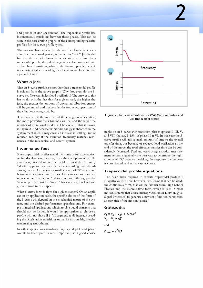
has to do with the fact that for a given load, the higher thejerk, the greater the amount of unwanted vibration energy will be generated, and the broader the frequency spectrum of the vibration’s energy will be.

This means that the more rapid the change in acceleration,the more powerful the vibrations will be, and the larger the

number of vibrational modes will be excited. This is shownin Figure 2. And because vibrational energy is absorbed in the

system mechanics, it may cause an increase in settling time orreduced accuracy if the vibration frequency matches reso-

nances in the mechanical and control system.

I wanna go fast

Since trapezoidal profiles spend their time at full accelerationor full deceleration, they are, from the standpoint of profileexecution, faster than S-curve profiles. But if this “all on”/

“all off ” approach causes an increase in settling time, the ad- vantage is lost. Often, only a small amount of “S” (transition

between acceleration and no acceleration) can substantially reduce induced vibration. And so to optimize throughput the

S-curve profile must be “tuned” for each a given load andgiven desired transfer speed.

What S-curve form is right for a given system? On an appli-cation by application basis, the specific choice of the form of the S-curve will depend on the mechanical nature of the sys-

tem, and the desired performance specifications. For exam-ple in medical applications which involve liquid transfers that

should not be jostled, it would be appropriate to choose aprofile with no phase II & VI segment at all, instead spread-

ing the acceleration transitions out as far as possible, thereby maximizing smoothness.

In other applications involving high speed pick and place,

overall transfer speed is most important, so a good choice

might be an S-curve with transition phases (phases I, III, V,

and VII) that are 5-15% of phase II & VI. In this case the S-curve profile will add a small amount of time to the overall

transfer time, but because of reduced load oscillation at theend of the move, the total effective transfer time can be con-

siderably decreased. Trial and error using a motion measure-ment system is generally the best way to determine the rightamount of “S,” because modelling the response to vibrations

is complicated, and not always accurate.

Trapezoidal profile equations

The basic math required to execute trapezoidal profiles is

straghtforward. There, however, two forms that can be used;the continuous form, that will be familiar from High SchoolPhysics, and the discrete time form, which is used in most

motion systems that utilize microprocessors or DSPs (DigitalSignal Processor) to generate a new set of motion parameters

at each tick of the motion “clock.”

Continuous form

P T = P 0 + V 0T + 1/2AT 2

V T = V 0 + AT

and

P decel = V 2/2A

Figure 2. Induced vibrations for (2A) S-curve profile and

(2B) trapezoidal profile

Frequency

2A

Frequency

E n e r

g y

E n e r g y

2B



3Discrete time form

P T = P T + V T +1/2A

V T = V T +A

where:P0 and V 0, are the starting position and velocities

P T and V T, are the position and velocity at time T

A is the profile acceleration

S-Curve Profile Equations

Because they are third versus second-order curves, and be-

cause there are seven versus three separate motion segments,point-to-point S-curves are more complicated then Trape-

zoids. In particular it is not simple to calculate the stopping distance for a given set of profile values. Accordingly, many S-curve profiling systems restrict changes-on-the-fly, or do not

allow asymmetric profiles. These restrictions allow informa-

tion about how long, and over what distance, the profile pre- viously took to accelerate to determine when to startdecelerating.

Continuous form

P T = P 0 + V 0T + 1/2A0T 2 + 1/6JT 3

V T = V 0 + A0T + 1/2 JT 2

AT = A0 + JT

Discrete time form

P T = P T + V T +1/2AT + 1/6J

V T = V T +AT + 1/2JT AT = AT +JT

where

P0, V 0, and A0 are the starting position, velocity, and

accelerationsP T , V T, and A T are the position, velocity, and acceleration

at time T J is the profile jerk (time rate of change of acceleration)

Making your point-to-point

The ultimate goal of any profile is to match the motion system

characteristics to the desired application. Trapezoidal and S-curve profiles work well when the motion system’s torque re-

sponse curve is fairly flat. In other words, when the outputtorque does not vary that much over the range of velocities thesystem will be experiencing. This is true for most servo motor

systems, whether DC Brush or Brushless DC.

Step motors, however, do not have flat torque/speed curves. Torque output is non-linear, sometimes having a large drop at

a location called the “mid-range instability,” and generally hav-ing drop-off at higher velocities. Figure 3 gives examples of

typical torque/speed curves for servo and step-motor systems.

Mid-range instability occurs at the step frequency when themotor’s natural resonance frequency matches the current step

rate. To address mid-range instability, the most common tech-nique is to use a non-zero starting velocity. This means that the

profile instantly “jumps” to a programmed velocity upon ini-tial acceleration, and while decelerating. This is shown in Fig-ure 4. While crude, this technique sometimes provides better

results than a smooth ramp for zero, particularly for systemsthat do not use a microstepping drive technique.

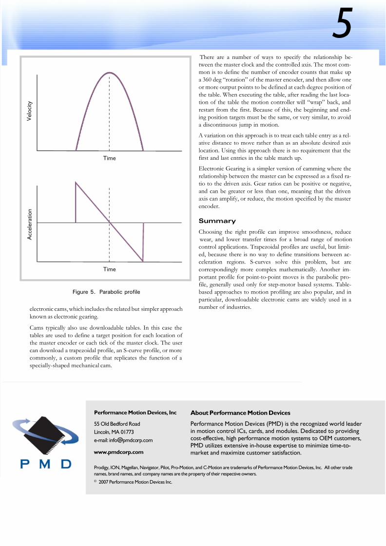
To address drop-off of torque at higher velocities, a Parabolic

profile, shown in Figure 5 can be used. The corresponding ac-celeration curve has the characteristic that the acceleration is

smallest when the velocity is highest. This is a good match forstep-motor systems, because there is less torque available athigher speeds. But notice that starting and ending accelerations

T o r q u e

T o r q u e

Speed

3A

Speed

3B

Figure 3. Typical torque/speed curves for (3A) servo and

(3B) step-motor systems



4

are very high, and there is no “S” phase where the accelerationsmoothly transitions to zero. So if load oscillation is a problem,

parabolic profiles may not work as well as an S-curve, despitethe fact that a standard S-curve profile is not optimized for a

step motor from the standpoint of the torque/speed curve.

Parabolic profile equations

Parabolic profiles are closely related to S-curves because they are third-order moves. And as was the case for S-curve pro-

files, calculating the distance to deceleration is complicated,particularly if profile changes-on-the-fly are allowed.

Continuous form

P T = P 0 + V 0T + 1/2A0T 2 - 1/6JT 3

V T = V 0 + A0T - 1/2 JT 2

AT = A0 - JT

Discrete time form

P T = P T + V T +1/2AT - 1/6JV T = V T +AT - 1/2JT

AT = AT - JT

where

P0, V 0, and A0 are the starting position, velocity, and

accelerationsP T , V T, and A T are the position, velocity, and

acceleration at time T J is the jerk (time rate of change of acceleration)

Table for 65,536 please

The ultimate in point-to-point profile generation, or in fact for

other types of profiles including continuous path generationsuch as is used in CNC (Computer Numerical Control) ma-

chine tools, is to construct a custom profile that compensatesfor the exact load and motor characteristics of the system.

Such a profile would accelerate the motor, taking into account

the available motor torque at each velocity point, the mechan-ical resonances at each velocity point, and the actuator or arm

kinematics in the mechanism.

Since motor torque curves do not follow simple mathematicalprinciples, and because the equations for kinematic compensa-

tion are complex, these calculations are generally calculated inadvance, and stored in a table of motion “vectors.” This table

is generally set up as an array of position or time vectors, witha corresponding entry for velocity and acceleration at each

point of the curve.

In this configuration the motion engine is merely providing a

generic capability to download and execute a list of vectors,

and the responsibility of the calculations falls to the user. De-spite this extra work, if special conditions exist, such as when

motors or mechanisms are highly non-linear, table-drivenpoint-to-point profiles can provide a meaningful performance

increase, and may be worth the effort.

Cam we talk?

Beyond point-to-point moves, there is a broad range of motion

applications that require repetitive motion, indexed by a mastertimer or encoder. Such applications fall under the category of

VelocityStarting

velocity

Starting

velocity

Time

V

A D

-V

-A -D

A = accelerationD = deceleration

V = velocity

Figure 4. Non-zero starting velocity



5

Performance Motion Devices, Inc

55 Old Bedford Road

Lincoln, MA 01773

e-mail: [email protected]

www.pmdcorp.com

About Performance Motion Devices

Performance Motion Devices (PMD) is the recognized world leaderin motion control ICs, cards, and modules. Dedicated to providingcost-effective, high performance motion systems to OEM customers,PMD utilizes extensive in-house expertise to minimize time-to-market and maximize customer satisfaction.

Prodigy, ION, Magellan, Navigator, Pilot, Pro-Motion, and C-Motion are trademarks of Performance Motion Devices, Inc. All other tradenames, brand names, and company names are the property of their respective owners.

© 2007 Performance Motion Devices Inc.

electronic cams, which includes the related but simpler approach

known as electronic gearing.

Cams typically also use downloadable tables. In this case the

tables are used to define a target position for each location of the master encoder or each tick of the master clock. The user

can download a trapezoidal profile, an S-curve profile, or morecommonly, a custom profile that replicates the function of a

specially-shaped mechanical cam.

There are a number of ways to specify the relationship be-tween the master clock and the controlled axis. The most com-mon is to define the number of encoder counts that make up

a 360 deg “rotation” of the master encoder, and then allow oneor more output points to be defined at each degree position of

the table. When executing the table, after reading the last loca-tion of the table the motion controller will “wrap” back, and

restart from the first. Because of this, the beginning and end-ing position targets must be the same, or very similar, to avoida discontinuous jump in motion.

A variation on this approach is to treat each table entry as a rel-ative distance to move rather than as an absolute desired axis

location. Using this approach there is no requirement that thefirst and last entries in the table match up.

Electronic Gearing is a simpler version of camming where the

relationship between the master can be expressed as a fixed ra-tio to the driven axis. Gear ratios can be positive or negative,

and can be greater or less than one, meaning that the drivenaxis can amplify, or reduce, the motion specified by the master

encoder.

Summary

Choosing the right profile can improve smoothness, reduce wear, and lower transfer times for a broad range of motioncontrol applications. Trapezoidal profiles are useful, but limit-

ed, because there is no way to define transitions between ac-celeration regions. S-curves solve this problem, but are

correspondingly more complex mathematically. Another im-

portant profile for point-to-point moves is the parabolic pro-

file, generally used only for step-motor based systems. Table-based approaches to motion profiling are also popular, and in

particular, downloadable electronic cams are widely used in anumber of industries.

Time

V e l o c i t y

Time

A c c e l e r a t i o n

Figure 5. Parabolic profile

Mathematics of Motion Control Profiles

Documents

Transcript of Mathematics of Motion Control Profiles