Brownian Motion and Ito’s Lemma - UT Mathematics Motion and Ito’s Lemma 1 Introduction 2...
42
Brownian Motion and Ito’s Lemma 1 Introduction 2 Geometric Brownian Motion 3 Ito’s Product Rule 4 Some Properties of the Stochastic Integral 5 Correlated Stock Prices 6 The Ornstein-Uhlenbeck Process
-
Upload
truongminh -
Category
Documents
-
view
227 -
download
5
Transcript of Brownian Motion and Ito’s Lemma - UT Mathematics Motion and Ito’s Lemma 1 Introduction 2...
Brownian Motion and Ito’s Lemma
1 Introduction
2 Geometric Brownian Motion
3 Ito’s Product Rule
4 Some Properties of the Stochastic Integral
5 Correlated Stock Prices
6 The Ornstein-Uhlenbeck Process
Brownian Motion and Ito’s Lemma
1 Introduction
2 Geometric Brownian Motion
3 Ito’s Product Rule
4 Some Properties of the Stochastic Integral
5 Correlated Stock Prices
6 The Ornstein-Uhlenbeck Process
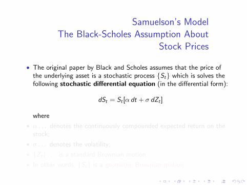
Samuelson’s ModelThe Black-Scholes Assumption About
Stock Prices
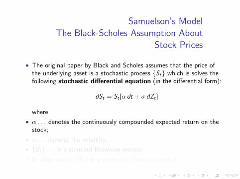
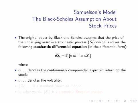
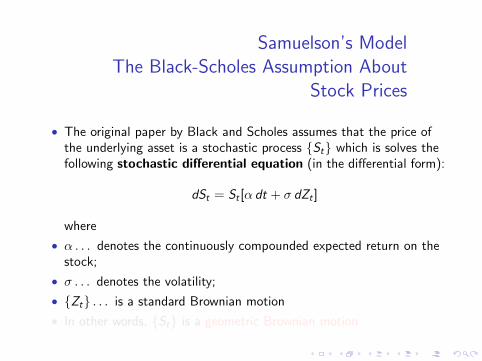
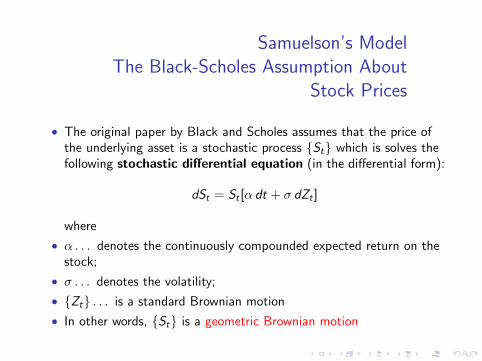
• The original paper by Black and Scholes assumes that the price ofthe underlying asset is a stochastic process {St} which is solves thefollowing stochastic differential equation (in the differential form):
dSt = St [α dt + σ dZt ]
where
• α . . . denotes the continuously compounded expected return on thestock;
• σ . . . denotes the volatility;
• {Zt} . . . is a standard Brownian motion
• In other words, {St} is a geometric Brownian motion
Samuelson’s ModelThe Black-Scholes Assumption About
Stock Prices
• The original paper by Black and Scholes assumes that the price ofthe underlying asset is a stochastic process {St} which is solves thefollowing stochastic differential equation (in the differential form):
dSt = St [α dt + σ dZt ]
where
• α . . . denotes the continuously compounded expected return on thestock;
• σ . . . denotes the volatility;
• {Zt} . . . is a standard Brownian motion
• In other words, {St} is a geometric Brownian motion
On the distribution of the stock price at agiven time
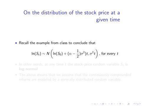
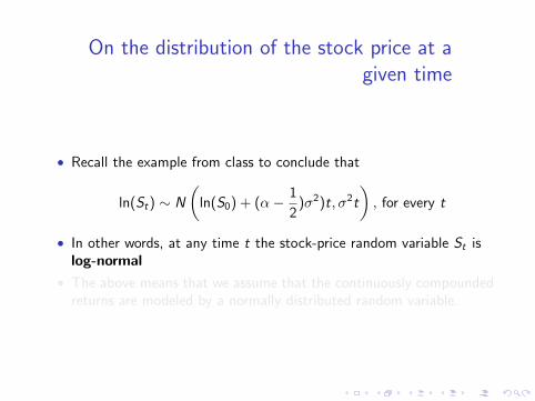
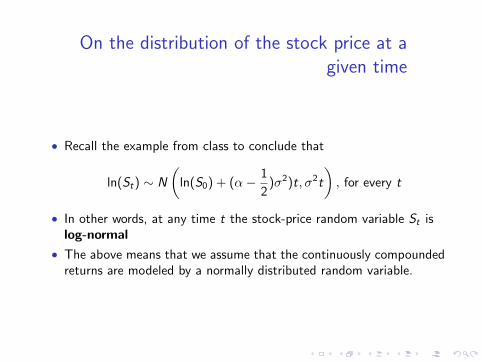
• Recall the example from class to conclude that
ln(St) ∼ N
(ln(S0) + (α− 1
2)σ2)t, σ2t
), for every t
• In other words, at any time t the stock-price random variable St islog-normal
• The above means that we assume that the continuously compoundedreturns are modeled by a normally distributed random variable.
On the distribution of the stock price at agiven time
• Recall the example from class to conclude that
ln(St) ∼ N
(ln(S0) + (α− 1
2)σ2)t, σ2t
), for every t
• In other words, at any time t the stock-price random variable St islog-normal
• The above means that we assume that the continuously compoundedreturns are modeled by a normally distributed random variable.
Brownian Motion and Ito’s Lemma
1 Introduction
2 Geometric Brownian Motion
3 Ito’s Product Rule
4 Some Properties of the Stochastic Integral
5 Correlated Stock Prices
6 The Ornstein-Uhlenbeck Process
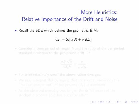
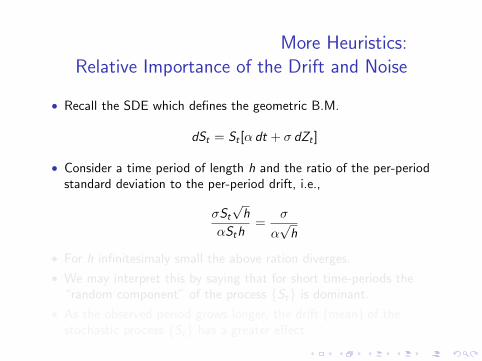
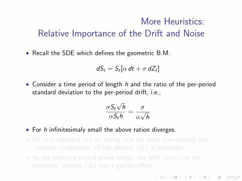
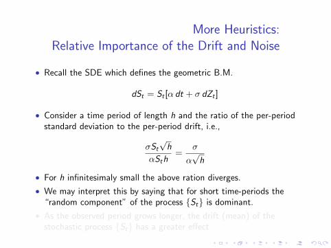
More Heuristics:Relative Importance of the Drift and Noise
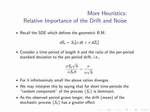
• Recall the SDE which defines the geometric B.M.
dSt = St [α dt + σ dZt ]
• Consider a time period of length h and the ratio of the per-periodstandard deviation to the per-period drift, i.e.,
σSt
√h
αSth=
σ
α√
h
• For h infinitesimaly small the above ration diverges.
• We may interpret this by saying that for short time-periods the“random component” of the process {St} is dominant.
• As the observed period grows longer, the drift (mean) of thestochastic process {St} has a greater effect
More Heuristics:Relative Importance of the Drift and Noise
• Recall the SDE which defines the geometric B.M.
dSt = St [α dt + σ dZt ]
• Consider a time period of length h and the ratio of the per-periodstandard deviation to the per-period drift, i.e.,
σSt
√h
αSth=
σ
α√
h
• For h infinitesimaly small the above ration diverges.
• We may interpret this by saying that for short time-periods the“random component” of the process {St} is dominant.
• As the observed period grows longer, the drift (mean) of thestochastic process {St} has a greater effect
Brownian Motion and Ito’s Lemma
1 Introduction
2 Geometric Brownian Motion
3 Ito’s Product Rule
4 Some Properties of the Stochastic Integral
5 Correlated Stock Prices
6 The Ornstein-Uhlenbeck Process
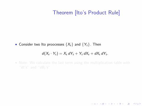
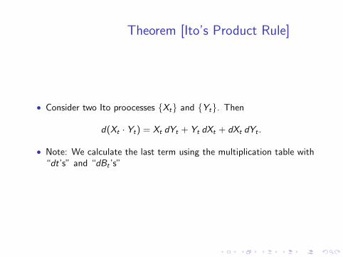
Theorem [Ito’s Product Rule]
• Consider two Ito proocesses {Xt} and {Yt}. Then
d(Xt · Yt) = Xt dYt + Yt dXt + dXt dYt .
• Note: We calculate the last term using the multiplication table with“dt’s” and “dBt ’s”
Theorem [Ito’s Product Rule]
• Consider two Ito proocesses {Xt} and {Yt}. Then
d(Xt · Yt) = Xt dYt + Yt dXt + dXt dYt .
• Note: We calculate the last term using the multiplication table with“dt’s” and “dBt ’s”
Brownian Motion and Ito’s Lemma
1 Introduction
2 Geometric Brownian Motion
3 Ito’s Product Rule
4 Some Properties of the Stochastic Integral
5 Correlated Stock Prices
6 The Ornstein-Uhlenbeck Process
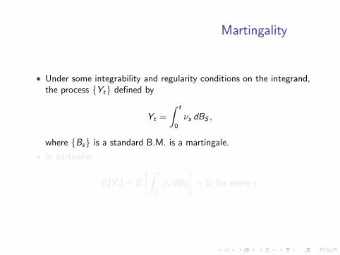
Martingality
• Under some integrability and regularity conditions on the integrand,the process {Yt} defined by
Yt =
∫ t
0
νs dBS ,
where {Bs} is a standard B.M. is a martingale.
• In particular
E[Yt ] = E[∫ t
0
νs dBS
]= 0, for every t
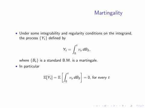
Martingality
• Under some integrability and regularity conditions on the integrand,the process {Yt} defined by
Yt =
∫ t
0
νs dBS ,
where {Bs} is a standard B.M. is a martingale.
• In particular
E[Yt ] = E[∫ t
0
νs dBS
]= 0, for every t
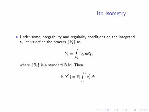
Ito Isometry
• Under some integrability and regularity conditions on the integrandν, let us define the process {Yt} as
Yt =
∫ t
0
νs dBS ,
where {Bs} is a standard B.M. Then
E[Y 2t ] = E[
∫ t
0
ν2s ds]
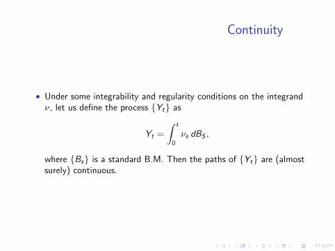
Continuity
• Under some integrability and regularity conditions on the integrandν, let us define the process {Yt} as
Yt =
∫ t
0
νs dBS ,
where {Bs} is a standard B.M. Then the paths of {Yt} are (almostsurely) continuous.
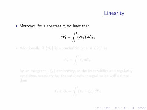
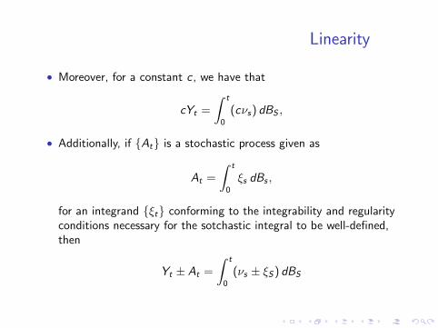
Linearity
• Moreover, for a constant c , we have that
cYt =
∫ t
0
(cνs) dBS ,
• Additionally, if {At} is a stochastic process given as
At =
∫ t
0
ξs dBs ,
for an integrand {ξt} conforming to the integrability and regularityconditions necessary for the sotchastic integral to be well-defined,then
Yt ± At =
∫ t
0
(νs ± ξS) dBS
Brownian Motion and Ito’s Lemma
1 Introduction
2 Geometric Brownian Motion
3 Ito’s Product Rule
4 Some Properties of the Stochastic Integral
5 Correlated Stock Prices
6 The Ornstein-Uhlenbeck Process
The Set-Up
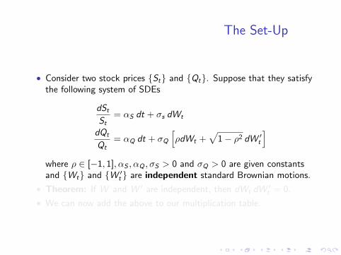
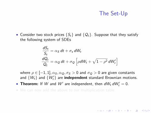
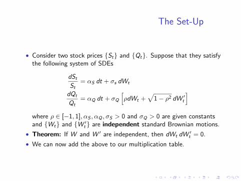
• Consider two stock prices {St} and {Qt}. Suppose that they satisfythe following system of SDEs
dSt
St= αS dt + σs dWt
dQt
Qt= αQ dt + σQ
[ρdWt +
√1− ρ2 dW ′
t
]where ρ ∈ [−1, 1], αS , αQ , σS > 0 and σQ > 0 are given constantsand {Wt} and {W ′
t } are independent standard Brownian motions.
• Theorem: If W and W ′ are independent, then dWt dW ′t = 0.
• We can now add the above to our multiplication table.
The Set-Up
• Consider two stock prices {St} and {Qt}. Suppose that they satisfythe following system of SDEs
dSt
St= αS dt + σs dWt
dQt
Qt= αQ dt + σQ
[ρdWt +
√1− ρ2 dW ′
t
]where ρ ∈ [−1, 1], αS , αQ , σS > 0 and σQ > 0 are given constantsand {Wt} and {W ′
t } are independent standard Brownian motions.
• Theorem: If W and W ′ are independent, then dWt dW ′t = 0.
• We can now add the above to our multiplication table.
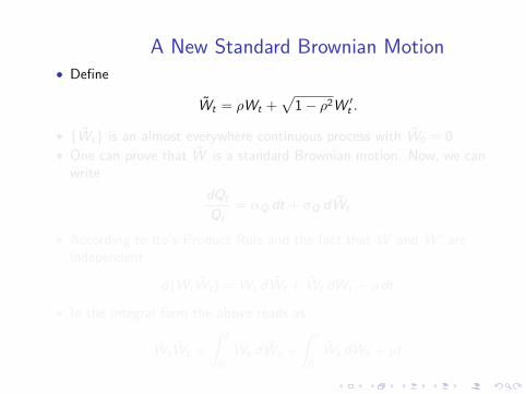
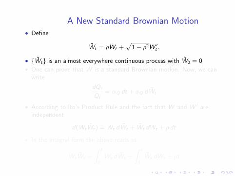
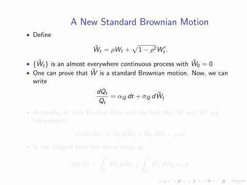
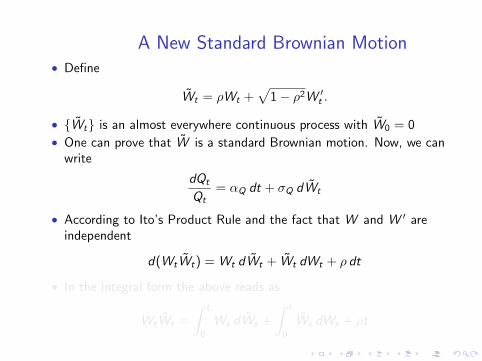
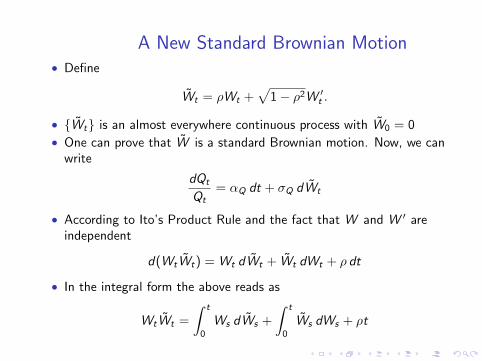
A New Standard Brownian Motion• Define
W̃t = ρWt +√
1− ρ2W ′t .
• {W̃t} is an almost everywhere continuous process with W̃0 = 0
• One can prove that W̃ is a standard Brownian motion. Now, we canwrite
dQt
Qt= αQ dt + σQ dW̃t
• According to Ito’s Product Rule and the fact that W and W ′ areindependent
d(WtW̃t) = Wt dW̃t + W̃t dWt + ρ dt
• In the integral form the above reads as
WtW̃t =
∫ t
0
Ws dW̃s +
∫ t
0
W̃s dWs + ρt
On the Correlation of the two BrownianMotions
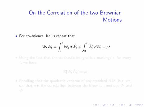
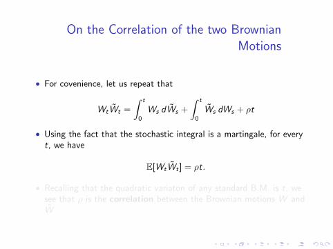
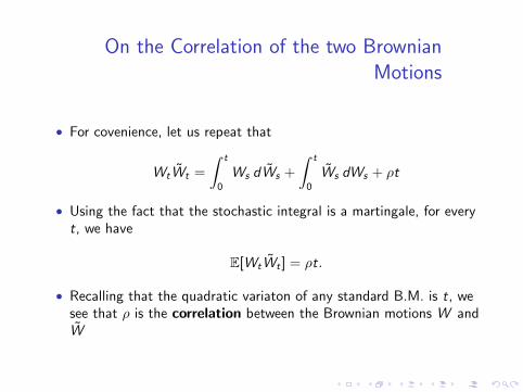
• For covenience, let us repeat that
WtW̃t =
∫ t
0
Ws dW̃s +
∫ t
0
W̃s dWs + ρt
• Using the fact that the stochastic integral is a martingale, for everyt, we have
E[WtW̃t ] = ρt.
• Recalling that the quadratic variaton of any standard B.M. is t, wesee that ρ is the correlation between the Brownian motions W andW̃
On the Correlation of the two BrownianMotions
• For covenience, let us repeat that
WtW̃t =
∫ t
0
Ws dW̃s +
∫ t
0
W̃s dWs + ρt
• Using the fact that the stochastic integral is a martingale, for everyt, we have
E[WtW̃t ] = ρt.
• Recalling that the quadratic variaton of any standard B.M. is t, wesee that ρ is the correlation between the Brownian motions W andW̃
Brownian Motion and Ito’s Lemma
1 Introduction
2 Geometric Brownian Motion
3 Ito’s Product Rule
4 Some Properties of the Stochastic Integral
5 Correlated Stock Prices
6 The Ornstein-Uhlenbeck Process
The Ornstein-Uhlenbeck Process
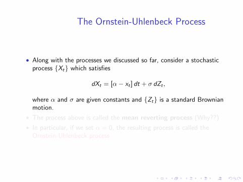
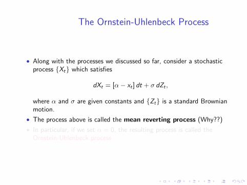
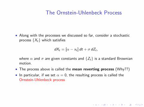
• Along with the processes we discussed so far, consider a stochasticprocess {Xt} which satisfies
dXt = [α− xt ] dt + σ dZt ,
where α and σ are given constants and {Zt} is a standard Brownianmotion.
• The process above is called the mean reverting process (Why??)
• In particular, if we set α = 0, the resulting process is called theOrnstein-Uhlenbeck process
The Ornstein-Uhlenbeck Process
• Along with the processes we discussed so far, consider a stochasticprocess {Xt} which satisfies
dXt = [α− xt ] dt + σ dZt ,
where α and σ are given constants and {Zt} is a standard Brownianmotion.
• The process above is called the mean reverting process (Why??)
• In particular, if we set α = 0, the resulting process is called theOrnstein-Uhlenbeck process