MatchIt: Nonparametric Preprocessing for Parametric Causal ... · MatchIt is an R program, and also...

JSS Journal of Statistical SoftwareMay 2011, Volume 42, Issue 8. http://www.jstatsoft.org/

MatchIt: Nonparametric Preprocessing for

Parametric Causal Inference

Daniel E. HoStanford Law School

Kosuke ImaiPrinceton University

Gary KingHarvard University

Elizabeth A. StuartJohns Hopkins University

Abstract

MatchIt implements the suggestions of Ho, Imai, King, and Stuart (2007) for improv-ing parametric statistical models by preprocessing data with nonparametric matchingmethods. MatchIt implements a wide range of sophisticated matching methods, makingit possible to greatly reduce the dependence of causal inferences on hard-to-justify, butcommonly made, statistical modeling assumptions. The software also easily fits into ex-isting research practices since, after preprocessing data with MatchIt, researchers can usewhatever parametric model they would have used without MatchIt, but produce infer-ences with substantially more robustness and less sensitivity to modeling assumptions.MatchIt is an R program, and also works seamlessly with Zelig.

Keywords: matching methods, causal inference, balance, preprocessing, R.

1. Introduction

1.1. What MatchIt does

MatchIt implements the suggestions of Ho, Imai, King, and Stuart (2007) for improvingparametric statistical models and reducing model dependence by preprocessing data withsemi-parametric and non-parametric matching methods. After appropriately preprocessingdata with MatchIt, researchers can use whatever parametric model and software they wouldhave used without MatchIt, without other modification, and produce inferences that aremore robust and less sensitive to modeling assumptions. MatchIt reduces the dependence of

http://www.jstatsoft.org/

2 MatchIt: Nonparametric Preprocessing for Parametric Causal Inference

causal inferences on commonly made, but hard-to-justify, statistical modeling assumptionsvia the largest range of sophisticated matching methods of any software we know of. Theprogram includes most existing approaches to matching and even enables users to accessmethods implemented in other programs through its single, unified, and easy-to-use interface.In addition, we have written MatchIt so that adding new matching methods to the softwareis as easy for anyone with the inclination as it is for us.

1.2. Software requirements

MatchIt works in conjunction with the R programming language and statistical software RDevelopment Core Team (2011) and will run on any platform where R is installed (Windows,Unix, or Mac OS X). MatchIt is available from the Comprehensive R Archive Network athttp://CRAN.R-project.org/package=MatchIt. MatchIt has been tested on the most re-cent version of R. A good way to learn R, if you do not know it already, is to learn Zelig whichincludes a self-contained introduction to R and can be used to analyze the matched data afterrunning MatchIt (Imai, King, and Lau 2011, 2008a).

2. Overview

MatchIt is designed for causal inference with a dichotomous treatment variable and a set ofpretreatment control variables. Any number or type of dependent variables can be used. (Ifyou are interested in the causal effect of more than one variable in your data set, run MatchItseparately for each one; it is unlikely that any one parametric model will produce valid causalinferences for more than one treatment variable at a time.) MatchIt can be used for othertypes of causal variables by dichotomizing them, perhaps in multiple ways (see also Imai andvan Dyk 2004). MatchIt works for experimental data, but is usually used for observationalstudies where the treatment variable is not randomly assigned by the investigator, or therandom assignment goes awry.

We adopt the same notation as in Ho, Imai, King, and Stuart (2007). Unless otherwise noted,let i index the n units in the data set, n1 denote the number of treated units, n0 denote thenumber of control units (such that n = n0 + n1), and xi indicate a vector of pretreatment(or control) variables for unit i. Let ti = 1 when unit i is assigned treatment, and ti = 0when unit i is assigned control. (The labels “treatment” and “control” and values 1 and 0respectively are arbitrary and can be switched for convenience, except that some methodsof matching are keyed to the definition of the treated group.) Denote yi(1) as the potentialoutcome of unit i under treatment — the value the outcome variable would take if ti wereequal to 1, whether or not ti in fact is 0 or 1 – and yi(0) the potential outcome of unit iunder control — the value the outcome variable would take if ti were equal to 0, regardlessof its value in fact. The variables yi(1) and yi(0) are jointly unobservable, and for each i, weobserve one yi = tiyi(1) + (1− ti)yi(0), and not the other.

Also denote a fixed vector of exogenous confounders (measured at pretreatment) as Xi. Thesevariables are defined in the hope or under the assumption that conditioning on them appro-priately will make inferences ignorable; see Ho, Imai, King, and Stuart (2007) for details.Measures of balance should be computed with respect to all of X, even if some methods ofmatching only use some components.

http://CRAN.R-project.org/package=MatchIt

Journal of Statistical Software 3

2.1. Preprocessing via matching

If ti and Xi were independent, we would not need to control for Xi, and any parametricanalysis would effectively reduce to a difference in means of Y for the treated and controlgroups. The goal of matching is to preprocess the data prior to the parametric analysis sothat the actual relationship between ti and Xi is eliminated or reduced without introducingbias and or increasing inefficiency too much.

When matching we select, duplicate, or selectively drop observations from our data, and wedo so without inducing bias as long as we use a rule that is a function only of ti and Xi anddoes not depend on the outcome variable Yi. Many methods that offer this preprocessingare included here, including exact, subclassification, nearest neighbor, optimal, and geneticmatching. For many of these methods the propensity score — defined as the probability ofreceiving the treatment given the covariates — is a key tool. In order to avoid changing thequantity of interest, most MatchIt routines work by retaining all treated units and selecting(or weighting) control units to include in the final data set; this enables one to estimate theaverage treatment effect on the treated (the purpose of which is described in Section 2.3).

MatchIt implements and evaluates the choice of the rules for matching. Matching sometimesincreases efficiency by eliminating heterogeneity or deleting observations outside of an areawhere a model can reasonably be used to extrapolate, but one needs to be careful not to losetoo many observations in matching or efficiency will drop more than the reduction in biasthat is achieved.

The simplest way to obtain good matches (as defined above) is to use one-to-one exact match-ing, which pairs each treated unit with one control unit for which the values of Xi are identi-cal. However, with many covariates and finite numbers of potential matches, sufficient exactmatches often cannot be found. Indeed, many of the other methods implemented in MatchItattempt to balance the overall covariate distributions as much as possible, when sufficientone-to-one exact matches are not available.

A key point in Ho, Imai, King, and Stuart (2007) is that matching methods by themselves arenot methods of estimation: every use of matching in the literature involves an analysis stepfollowing the matching procedure, but almost all analyses use a simple difference in means.This procedure is appropriate only if exact matching was conducted. In almost all other cases,some adjustment is required, and there is no reason to degrade your inferences by using aninferior method of analysis such as a difference in means even when improving your inferencesvia preprocessing. Thus, with MatchIt, you can improve your analyses in two ways. MatchItanalyses are “doubly robust” in that if either the matching analysis or the analysis model iscorrect (but not necessarily both) your inferences will be statistically consistent. In practice,the modeling choices you make at the analysis stage will be much less consequential if youmatch first.

2.2. Checking balance

The goal of matching is to create a data set that looks closer to one that would result from aperfectly blocked (and possibly randomized) experiment. When we get close to attaining thisgoal, we break the link between the treatment variable and the pre-treatment controls, whichmakes the parametric form of the analysis model less relevant or irrelevant entirely. To breakthis link, we need the distribution of covariates to be the same within the matched treatedand control groups.


A crucial part of any matching procedure is, therefore, to assess how close the (empirical)covariate distributions are in the two groups, which is known as “balance.” Because theoutcome variable is not used in the matching procedure, any number of matching methodscan be tried and evaluated, and the one matching procedure that leads to the best balancecan be chosen.

MatchIt provides a number of ways to assess the balance of covariates after matching, includ-ing numerical summaries such as the mean Diff. (difference in means) or the difference inmeans divided by the treated group standard deviation, and summaries based on quantile-quantile plots that compare the empirical distributions of each covariate. The widely usedprocedure of doing t-tests of the difference in means is highly misleading and should never beused to assess balance; see Imai, King, and Stuart (2008b). These balance diagnostics shouldbe performed on all variables in X, even if some are excluded from one of the matchingprocedures.

2.3. Conducting analyses after matching

The most common way that parametric analyses are used to compute quantities of interest(without matching) is by (statistically) holding constant some explanatory variables, changingothers, and computing predicted or expected values and taking the difference or ratio, all byusing the parametric functional form. In the case of causal inference, this would mean lookingat the effect on the expected value of the outcome variable when changing T from 0 to 1,while holding constant the pretreatment control variables X at their means or medians. This,and indeed any other appropriate analysis procedure, would be a perfectly reasonable way toproceed with analysis after matching. If it is the chosen way to proceed, then either treated orcontrol units may be deleted during the matching stage, since the same parametric structureis assumed to apply to all observations.

In other instances, researchers wish to reduce the assumptions inherent in their statisticalmodel and so want to allow for the possibility that their treatment effect varies over observa-tions. In this situation, one popular quantity of interest used is the average treatment effect onthe treated (ATT). For example, for the treated group, the potential outcomes under control,Yi(0), are missing, whereas the outcomes under treatment, Yi(1), are observed, and the goalof the analysis is to impute the missing outcomes, Yi(0) for observations with Ti = 1. Wedo this via simulation using a parametric statistical model such as linear regression, logit, orothers (as described below). Once those potential outcomes are imputed from the model, theestimate of individual i’s treatment effect is Yi(1)− Yi(0) where Yi(0) is a predicted value ofthe dependent variable for unit i under the counterfactual condition where Ti = 0. The in-sample average treatment effect for the treated individuals can then be obtained by averagingthis difference over all observations i where in fact Ti = 1. Most MatchIt algorithms retainall treated units, and choose some subset of or repeated units from the control group, sothat estimating the ATT is straightforward. If one chooses options that allow matching withreplacement, or any solution that has different numbers of controls (or treateds) within eachsubclass or strata (such as full matching), then the parametric analysis following matchingmust accommodate these procedures, such as by using fixed effects or weights, as appropriate.(Similar procedures can also be used to estimate various other quantities of interest such asthe average treatment effect by computing it for all observations, but then one must be awarethat the quantity of interest may change during the matching procedure as some control units


may be dropped.)

The imputation from the model can be done in at least two ways. Recall that the model isused to impute the value that the outcome variable would take among the treated units if thosetreated units were actually controls. Thus, one reasonable approach would be to fit a modelto the matched data and create simulated predicted values of the dependent variable for thetreated units with Ti switched counterfactually from 1 to 0. An alternative approach would beto fit a model without T by using only the outcomes of the matched control units (i.e., usingonly observations where Ti = 0). Then, given this fitted model, the missing outcomes Yi(0)are imputed for the matched treated units by using the values of the explanatory variables forthe treated units. The first approach will usually have lower variance, since all observationsare used, and the second may have less bias, since no assumption of constant parametersacross the models of the potential outcomes under treatment and control is needed. See Ho,Imai, King, and Stuart (2007) for more details.

Other quantities of interest can also be computed at the parametric stage, following anyprocedures you would have followed in the absence of matching. The advantage is that ifmatching is done well your answers will be more robust to many small changes in parametricspecification.

3. User’s guide to MatchIt

3.1. Preprocessing via matching

Quick overview

The main command matchit() implements the matching procedures. A general syntax is:

R> m.out <- matchit(treat ~ x1 + x2, data = mydata)

where treat is the dichotomous treatment variable, and x1 and x2 are pre-treatment co-variates, all of which are contained in the data frame mydata. The dependent variable (orvariables) may be included in mydata for convenience but is never used by MatchIt or includedin the formula. This command creates the MatchIt object called m.out. Passing the name ofthe object will produce a quick summary of the results:

R> m.out

Examples

To run any of the examples below, you first must load the library and and data:

R> library("MatchIt")

R> data("lalonde")

Our example data set is a subset of the job training program analyzed in Lalonde (1986)and Dehejia and Wahba (1999). MatchIt includes a subsample of the original data consisting


of the National Supported Work Demonstration (NSW) treated group and the comparisonsample from the Population Survey of Income Dynamics (PSID).1 The variables in this dataset include participation in the job training program (treat, which is equal to 1 if participatedin the program, and 0 otherwise), age (age), years of education (educ), race (black which isequal to 1 if black, and 0 otherwise; hispan which is equal to 1 if hispanic, and 0 otherwise),marital status (married, which is equal to 1 if married, 0 otherwise), high school degree(nodegree, which is equal to 1 if no degree, 0 otherwise), 1974 real earnings (re74), 1975 realearnings (re75), and the main outcome variable, 1978 real earnings (re78).

Exact matching

The simplest version of matching is exact. This technique matches each treated unit to allpossible control units with exactly the same values on all the covariates, forming subclassessuch that within each subclass all units (treatment and control) have the same covariate values.Exact matching is implemented in MatchIt using method = "exact". Exact matching will bedone on all covariates included on the right-hand side of the formula specified in the MatchItcall. There are no additional options for exact matching. (Exact restrictions on a subsetof covariates can also be specified in nearest neighbor matching; see below.) The followingexample can be run by typing demo("exact") at the R prompt,

R> m.out <- matchit(treat ~ educ + black + hispan, data = lalonde,

+ method = "exact")

Subclassification

When there are many covariates (or some covariates can take a large number of values),finding sufficient exact matches will often be impossible. The goal of subclassification is toform subclasses, such that in each the distribution (rather than the exact values) of covariatesfor the treated and control groups are as similar as possible. Various subclassification schemesexist, including the one based on a scalar distance measure such as the propensity scoreestimated using the distance option (see Section 4.1.3). Subclassification is implemented inMatchIt using method = "subclass".

The following example script can be run by typing demo("subclass") at the R prompt,

R> m.out <- matchit(treat ~ re74 + re75 + educ + black + hispan + age,

+ data = lalonde, method = "subclass")

The above syntax forms 6 subclasses, which is the default number of subclasses, based on adistance measure (the propensity score) estimated using logistic regression. By default, eachsubclass will have approximately the same number of treated units.

Subclassification may also be used in conjunction with nearest neighbor matching describedbelow, by leaving the default of method = "nearest" but adding the option subclass. Whenyou choose this option, MatchIt selects matches using nearest neighbor matching, but afterthe nearest neighbor matches are chosen it places them into subclasses, and adds a variableto the output object indicating subclass membership.

1This data set, lalonde, was created using NSWRE74_TREATED.TXT and CPS3_CONTROLS.TXT.


Nearest neighbor matching

Nearest neighbor matching selects the r (default = 1) best control matches for each individualin the treatment group (excluding those discarded using the discard option). Matching isdone using a distance measure specified by the distance option (default = logit, i.e., alogistic regression model is used to estimate the propensity score, defined as the probabilityof receiving treatment, conditional on the covariates). Matches are chosen for each treatedunit one at a time, with the order specified by the m.order command (default = largest tosmallest). At each matching step we choose the control unit that is not yet matched but isclosest to the treated unit on the distance measure.

Nearest neighbor matching is implemented in MatchIt using the method = "nearest" option.The following example script can be run by typing demo("nearest"):

R> m.out <- matchit(treat ~ re74 + re75 + educ + black + hispan + age,

+ data = lalonde, method = "nearest")

Optimal matching

The default nearest neighbor matching method in MatchIt is “greedy” matching, where theclosest control match for each treated unit is chosen one at a time, without trying to minimizea global distance measure. In contrast, “optimal”matching finds the matched samples with thesmallest average absolute distance across all the matched pairs. Gu and Rosenbaum (1993)find that greedy and optimal matching approaches generally choose the same sets of controlsfor the overall matched samples, but optimal matching does a better job of minimizing thedistance within each pair. In addition, optimal matching can be helpful when there are notmany appropriate control matches for the treated units.

Optimal matching is performed with MatchIt by setting method = "optimal", which auto-matically loads an add-on package called optmatch (Hansen 2004). The following examplecan also be run by typing demo("optimal") at the R prompt. We conduct 2:1 optimal ratiomatching based on the propensity score from the logistic regression.

R> m.out <- matchit(treat ~ re74 + re75 + age + educ, data = lalonde,

+ method = "optimal", ratio = 2)

Full matching

Full matching is a particular type of subclassification that forms the subclasses in an optimalway (Rosenbaum 2002; Hansen 2004). A fully matched sample is composed of matched sets,where each matched set contains one treated unit and one or more controls (or one controlunit and one or more treated units). As with subclassification, the only units not placed intoa subclass will be those discarded (if a discard option is specified) because they are outsidethe range of common support. Full matching is optimal in terms of minimizing a weightedaverage of the estimated distance measure between each treated subject and each controlsubject within each subclass.

Full matching can be performed with MatchIt by setting method = "full". Just as withoptimal matching, we use the optmatch package (Hansen 2004), which automatically loadswhen needed. The following example with full matching (using the default propensity scorebased on logistic regression) can also be run by typing demo("full") at the R prompt:


R> m.out <- matchit(treat ~ age + educ + black + hispan + married +

+ nodegree + re74 + re75, data = lalonde, method = "full")

Genetic matching

Genetic matching automates the process of finding a good matching solution (Diamond andSekhon 2010). The idea is to use a genetic search algorithm to find a set of weights foreach covariate such that the a version of optimal balance is achieved after matching. Ascurrently implemented, matching is done with replacement using the matching method ofAbadie and Imbens (2006) and balance is determined by two univariate tests, paired t-testsfor dichotomous variables and a Kolmogorov-Smirnov test for multinomial and continuousvariables, but these options can be changed.

Genetic matching can be performed with MatchIt by setting method = "genetic", whichautomatically loads the Matching (Sekhon 2011) package. The following example of geneticmatching (using the estimated propensity score based on logistic regression as one of thecovariates) can also be run by typing demo("genetic"):

R> m.out <- matchit(treat ~ age + educ + black + hispan + married +

+ nodegree + re74 + re75, data = lalonde, method = "genetic")

3.2. Checking balance

Quick overview

To check balance, use summary(m.out) for numerical summaries and plot(m.out) for graph-ical summaries.

The summary() command

The summary() command gives measures of the balance between the treated and controlgroups in the full (original) data set, and then in the matched data set. If the matchingworked well, the measures of balance should be smaller in the matched data set (smallervalues of the measures indicate better balance).

The summary() output for subclassification is the same as that for other types of matching,except that the balance statistics are shown separately for each subclass, and the overallbalance in the matched samples is calculated by aggregating across the subclasses, whereeach subclass is weighted by the number of units in the subclass. For exact matching, thecovariate values within each subclass are guaranteed to be the same, and so the measures ofbalance are not output for exact matching; only the sample sizes in each subclass are shown.

� Balance statistics: The statistics the summary() command provides include means,the original control group standard deviation (where applicable), mean differences, stan-dardized mean differences, and (median, mean and maximum) quantile-quantile (Q-Q)plot differences. In addition, the summary() command will report (a) the matched call,(b) how many units were matched, unmatched, or discarded due to the discard option(described below), and (c) the percent improvement in balance for each of the balance


measures, defined as 100((|a| − |b|)/|a|), where a is the balance before and b is the bal-ance after matching. For each set of units (original and matched data sets, with weightsused as appropriate in the matched data sets), the following statistics are provided:

1. Means Treated and Means Control show the weighted means in the treated andcontrol groups

2. SD Control is the standard deviation calculated in the control group (where ap-plicable)

3. Mean Diff. is the difference in means between the groups

4. The final three columns of the summary output give summary statistics of a Q-Qplot (see below for more information on these plots). Those columns give the me-dian, mean, and maximum distance between the two empirical quantile functions(treated and control groups). Values greater than 0 indicate deviations betweenthe groups in some part of the empirical distributions. The plots of the two empiri-cal quantile functions themselves, described below, can provide further insight intowhich part of the covariate distribution has differences between the two groups.

� Additional options: Three options to the summary() command can also help withassessing balance and respecifying the propensity score model, as necessary. First, theinteractions = TRUE option with summary() shows the balance of all squares andinteractions of the covariates used in the matching procedure. Large differences inhigher order interactions usually are a good indication that the propensity score model(the distance measure) needs to be respecified. Similarly, the addlvariables optionwith summary() will provide balance measures on additional variables not included in theoriginal matching procedure. If a variable (or interaction of variables) not included in theoriginal propensity score model has large imbalances in the matched groups, includingthat variable in the next model specification may improve the resulting balance on thatvariable. Because the outcome variable is not used in the matching procedure, a varietyof matching methods can be tried, and the one that leads to the best resulting balancechosen. Finally, the standardize = TRUE option will print out standardized versionsof the balance measures, where the mean difference is standardized (divided) by thestandard deviation in the original treated group.

The plot() command

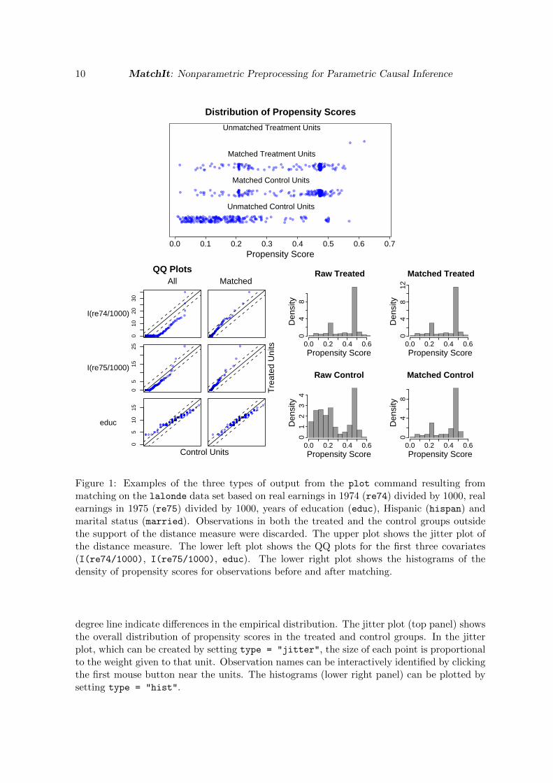
We can also examine the balance graphically using the plot() command, which providesthree types of plots: jitter plots of the distance measure, Q-Q plots of each covariate, andhistograms of the distance measure. For subclassification, separate Q-Q plots can be printedfor each subclass. The jitter plot for subclassification is the same as that for other typesof matching, with the addition of vertical lines indicating the subclass cut-points. With thehistogram option, 4 histograms are provided: the original treated and control groups and thematched treated and control groups. For the Q-Q plots and the histograms, the weights thatresult after matching are used to create the plots.

Three examples of the output from the plot() command are shown in Figure 1. If theempirical distributions are the same in the treated and control groups, the points in the Q-Qplots would all lie on the 45 degree line (lower left panel of Figure 1). Deviations from the 45


Distribution of Propensity Scores

Propensity Score0.0 0.1 0.2 0.3 0.4 0.5 0.6 0.7

Unmatched Treatment Units

Matched Treatment Units

Matched Control Units

Unmatched Control Units

Index

QQ PlotsAll Matched

Control Units

Tre

ated

Uni

ts

I(re74/1000)

010

2030

Index

I(re75/1000)

05

1525

educ

05

1015

Raw Treated

Propensity Score

Den

sity

0.0 0.2 0.4 0.6

04

8

Matched Treated

Propensity Score

Den

sity

0.0 0.2 0.4 0.6

04

812

Raw Control

Propensity Score

Den

sity

0.0 0.2 0.4 0.6

01

23

4

Matched Control

Propensity Score

Den

sity

0.0 0.2 0.4 0.6

04

8

Figure 1: Examples of the three types of output from the plot command resulting frommatching on the lalonde data set based on real earnings in 1974 (re74) divided by 1000, realearnings in 1975 (re75) divided by 1000, years of education (educ), Hispanic (hispan) andmarital status (married). Observations in both the treated and the control groups outsidethe support of the distance measure were discarded. The upper plot shows the jitter plot ofthe distance measure. The lower left plot shows the QQ plots for the first three covariates(I(re74/1000), I(re75/1000), educ). The lower right plot shows the histograms of thedensity of propensity scores for observations before and after matching.

degree line indicate differences in the empirical distribution. The jitter plot (top panel) showsthe overall distribution of propensity scores in the treated and control groups. In the jitterplot, which can be created by setting type = "jitter", the size of each point is proportionalto the weight given to that unit. Observation names can be interactively identified by clickingthe first mouse button near the units. The histograms (lower right panel) can be plotted bysetting type = "hist".


3.3. Conducting analyses after matching

Any software package may be used for parametric analysis following MatchIt. This includesany of the relevant R packages, or other statistical software by exporting the resulting matcheddata sets using R commands such as write.csv() and write.table() for ASCII files orwrite.dta() in the foreign package for a Stata binary file.

When variable numbers of treated and control units have been matched to each other (e.g.,through exact matching, full matching, or k:1 matching with replacement), the weights createdby MatchIt should be used (e.g., in a weighted regression) to ensure that the matched treatedand control groups are weighted up to be similar. Users should also remember that theweights created by MatchIt estimate the average treatment effect on the treated, with thecontrol units weighted to resemble the treated units. See below for more detail on the weights.With subclassification, estimates should be obtained within each subclass and then aggregatedacross subclasses. When it is not possible to calculate an effect within each subclass, againthe weights can be used to weight the matched units.

In this section, we show how to use Zelig with MatchIt.Zelig (Imai, King, and Lau 2011) isan R package that implements a large variety of statistical models (using numerous existing Rpackages) with a single easy-to-use interface, gives easily interpretable results by simulatingquantities of interest, provides numerical and graphical summaries, and is easily extensible toinclude new methods.

Quick overview

The general syntax is as follows. First, we use match.data() to create the matched data fromthe MatchIt output object (m.out) by excluding unmatched units from the original data, andincluding information produced by the particular matching procedure (i.e., primarily a newdata set, but also information that may result such as weights, subclasses, or the distancemeasure).

R> m.data <- match.data(m.out)

where m.data is the resulting matched data. Zelig analyses all use three commands — zelig,setx, and sim. For example, the basic statistical analysis is performed first:

R> z.out <- zelig(Y ~ treat + x1 + x2, model = mymodel, data = m.data)

where Y is the outcome variable, mymodel is the selected model, and z.out is the outputobject from zelig. This output object includes estimated coefficients, standard errors, andother typical outputs from your chosen statistical model. Its contents can be examined viasummary(z.out) or plot(z.out), but the idea of Zelig is that these statistical results aretypically only intermediate quantities needed to compute your ultimate quantities of interest,which in the case of matching are usually causal inferences. To get these causal quantities, weuse Zelig’s other two commands. Thus, we can set the explanatory variables at their means(the default) and change the treatment variable from a 0 to a 1:

R> x.out0 <- setx(z.out0, treat = 0)

R> x1.out0 <- setx(z.out0, treat = 1)

and finally compute the resulting estimates of the causal effects and examine a summary:


R> s.out0 <- sim(z.out1, x = x.out1)

R> summary(s.out0)

Examples

We now give four examples using the Lalonde data. They are meant to be read sequentially.You can run these example commands by typing demo("analysis"). Although we use thelinear least squares model in these examples, a wide range of other models are availablein Zelig (for the list of supported models, see http://gking.harvard.edu/zelig/docs/

Models_Zelig_Can.html).

To load the Zelig package after installing it, type

R> library("Zelig")

Model-based estimates In our first example, we conduct a standard parametric analysisand compute quantities of interest in the most common way. We begin with nearestneighbor matching with a logistic regression-based propensity score, discarding with thehull.control option (King and Zeng 2006, 2007):

R> m.out0 <- matchit(treat ~ age + educ + black + hispan + nodegree +

+ married + re74 + re75, method = "nearest", discard = "hull.control",

+ data = lalonde)

Then we check balance using the summary and plot procedures (which we do not showhere). When the best balance is achieved, we run the parametric analysis (two variablesare dropped because they are exactly matched):

R> z.out0 <- zelig(re78 ~ treat + age + educ + black + nodegree +

+ re74 + re75, data = match.data(m.out0), model = "ls")

and then set the explanatory variables at their means (the default) and change thetreatment variable from a 0 to a 1:

R> x.out0 <- setx(z.out0, treat = 0)

R> x1.out0 <- setx(z.out0, treat = 1)

and finally compute the result and examine a summary:

R> s.out0 <- sim(z.out0, x = x.out0, x1 = x1.out0)

R> summary(s.out0)

Average treatment effect on the treated We illustrate now how to estimate the averagetreatment effect on the treated in a way that is quite robust. We do this by estimatingthe coefficients in the control group alone.

We begin by conducting nearest neighbor matching with a logistic regression-basedpropensity score:


+ married + re74 + re75, method = "nearest", data = lalonde)

http://gking.harvard.edu/zelig/docs/Models_Zelig_Can.html

http://gking.harvard.edu/zelig/docs/Models_Zelig_Can.html


Then we check balance using the summary and plot procedures (which we do not showhere). We reestimate the matching procedure until we achieve the best balance possible.The running examples here are meant merely to illustrate, not to suggest that we’veachieved the best balance. Then we go to Zelig, and in this case choose to fit a linearleast squares model to the control group only:

R> z.out1 <- zelig(re78 ~ age + educ + black + hispan + nodegree +

+ married + re74 + re75, data = match.data(m.out1, "control"),

+ model = "ls")

where the "control" option in match.data() extracts only the matched control unitsand ls specifies least squares regression. In a smaller data set, this example should prob-ably be changed to include all the data in this estimation (using data =

match.data(m.out1) for the data) and by including the treatment indicator (whichis excluded in the example since its a constant in the control group.) Next, we use thecoefficients estimated in this way from the control group, and combine them with thevalues of the covariates set to the values of the treated units. We do this by choosingconditional prediction (which means use the observed values) in setx(). The sim()

command does the imputation.

R> x.out1 <- setx(z.out1, data = match.data(m.out1, "treat"),

+ cond = TRUE)


Finally, we obtain a summary of the results by

R> summary(s.out1)

Average treatment effect (overall) To estimate the average treatment effect, we continuewith the previous example and fit the linear model to the treatment group:

R> z.out2 <- zelig(re78 ~ age + educ + black + hispan + nodegree +

+ married + re74 + re75, data = match.data(m.out1, "treat"),

+ model = "ls")

We then conduct the same simulation procedure in order to impute the counterfactualoutcome for the control group,

R> x.out2 <- setx(z.out2, data = match.data(m.out1, "control"),

+ cond = TRUE)


In this calculation, Zelig is computing the difference between observed and the expectedvalues. This means that the treatment effect for the control units is the effect of con-trol (observed control outcome minus the imputed outcome under treatment from themodel). Hence, to combine treatment effects just reverse the signs of the estimatedtreatment effect of controls.

R> ate.all <- c(s.out1$qi$att.ev, -s.out2$qi$att.ev)

The point estimate, its standard error, and the 95% confidence interval is given by


R> mean(ate.all)

R> sd(ate.all)

R> quantile(ate.all, c(0.025, 0.975))

Subclassification In subclassification, the average treatment effect estimates are obtainedseparately for each subclass, and then aggregated for an overall estimate. Estimatingthe treatment effects separately for each subclass, and then aggregating across sub-classes, can increase the robustness of the ultimate results since the parametric analysiswithin each subclass requires only local rather than global assumptions. However, fewerobservations are obviously available within each subclass, and so this option is normallychosen for larger data sets.

We begin this example by conducting subclassification with four subclasses,


+ married + re74 + re75, data = lalonde, method = "subclass",

+ subclass = 4)

When balance is as good as we can get it, we then fit a linear regression within eachsubclass by controlling for the estimated propensity score (called distance) and othercovariates. In most software, this would involve running four separate regressions andthen combining the results. In Zelig, however, all we need to do is to use the by option:

R> z.out3 <- zelig(re78 ~ re74 + re75 + distance, data =

+ match.data(m.out2, "control"), model = "ls", by = "subclass")

The same set of commands as in the first example are used to do the imputation of thecounterfactual outcomes for the treated units:

R> x.out3 <- setx(z.out3, data = match.data(m.out2, "treat"), fn = NULL,

+ cond = TRUE)


R> summary(s.out3)

It is also possible to get the summary result for each subclass. For example, the followingcommand summarizes the result for the second subclass.

R> summary(s.out3, subset = 2)

How adjustment after exact matching has no effect Regression adjustment after ex-act one-to-one exact matching gives the identical answer as a simple, unadjusted differ-ence in means. General exact matching, as implemented in MatchIt, allows one-to-manymatches, so to see the same result we must weight when adjusting. In other words:weighted regression adjustment after general exact matching gives the identical answeras a simple, unadjusted weighted difference in means. For example:

R> m.out <- matchit(treat ~ educ + black + hispan, data = lalonde,

+ method = "exact")

R> m.data <- match.data(m.out)

R> weighted.mean(m.data$re78[m.data$treat == 1],

+ m.data$weights[m.data$treat == 1]) -


+ weighted.mean(m.data$re78[m.data$treat == 0],

+ m.data$weights[m.data$treat == 0])

[1] 807

R> zelig(re78 ~ treat, data = m.data, model = "ls",

+ weights = "weights")

Call:

zelig(formula = re78 ~ treat, model = "ls", data = m.data,

weights = "weights")

Coefficients:

(Intercept) treat

5524 807

R> zelig(re78 ~ treat + black + hispan + educ, data = m.data,

+ model = "ls", weights = "weights")

Call:

zelig(formula = re78 ~ treat + black + hispan + educ, model = "ls",

data = m.data, weights = "weights")

Coefficients:

(Intercept) treat black hispan educ

314 807 -1882 258 657

4. Reference manual

4.1. matchit: Implementation of matching methods

Use matchit() to implement a variety of matching procedures including exact matching,nearest neighbor matching, subclassification, optimal matching, genetic matching, and fullmatching. The output of matchit() can be analyzed via any standard R package, by exportingthe data for use in another program, or most simply via Zelig in R.

Syntax

m.out <- matchit(formula, data, method = "nearest", verbose = FALSE, ...)

Arguments for all matching methods

� formula: formula used to calculate the distance measure for matching (e.g., the propen-sity score model). It takes the usual syntax of R formulas, treat ~ x1 + x2, where


treat is a binary treatment indicator, and x1 and x2 are the pre-treatment covari-ates. Both the treatment indicator and pre-treatment covariates must be containedin the same data frame, which is specified as data (see below). All of the usual Rsyntax for formulas work here. For example, x1:x2 represents the first order interac-tion term between x1 and x2, and I(x1 ^ 2) represents the square term of x1. Seehelp("formula") for details.

� data: the data frame containing the variables called in formula.

� method: the matching method (default = "nearest", nearest neighbor matching). Cur-rently, "exact" (exact matching), "full" (full matching), "nearest" (nearest neigh-bor matching), "optimal" (optimal matching), "subclass" (subclassification), and"genetic" (genetic matching) are available. Note that within each of these match-ing methods, MatchIt offers a variety of options. See below for more details.

� verbose: a logical value indicating whether to print the status of the matching algorithm(default = FALSE).

Additional arguments for specification of distance measures

The following arguments specify distance measures that are used for matching methods. Thesearguments apply to all matching methods except exact matching.

� distance: the method used to estimate the distance measure (default = "logit",logistic regression) or a numerical vector of user’s own distance measure. Before usingany of these techniques, it is best to understand the theoretical groundings of thesetechniques and to evaluate the results. Most of these methods (such as logistic or probitregression) define the distance by first estimating the propensity score, defined as theprobability of receiving treatment, conditional on the covariates. Available methodsinclude:

– "mahalanobis": the Mahalanobis distance measure.

– binomial generalized linear models with one of the following link functions:

* "logit": logistic link

* "linear.logit": logistic link with linear propensity score2

* "probit": probit link

* "linear.probit": probit link with linear propensity score

* "cloglog": complementary log-log link

* "linear.cloglog": complementary log-log link with linear propensity score

* "log": log link

* "linear.log": log link with linear propensity score

* "cauchit" Cauchy CDF link

* "linear.cauchit" Cauchy CDF link with linear propensity score

– Choose one of the following generalized additive models (see help("gam") for moreoptions).

2The linear propensity scores are obtained by transforming back onto a linear scale.


* "GAMlogit": logistic link

* "GAMlinear.logit": logistic link with linear propensity score

* "GAMprobit": probit link

* "GAMlinear.probit": probit link with linear propensity score

* "GAMcloglog": complementary log-log link

* "GAMlinear.cloglog": complementary log-log link with linear propensityscore

* "GAMlog": log link

* "GAMlinear.log": log link with linear propensity score,

* "GAMcauchit": Cauchy CDF link

* "GAMlinear.cauchit": Cauchy CDF link with linear propensity score

– "nnet": neural network model. See help("nnet") for more options.

– "rpart": classification trees. See help("rpart") for more options.

� distance.options: optional arguments for estimating the distance measure. The in-put to this argument should be a list. For example, if the distance measure is esti-mated with a logistic regression, users can increase the maximum IWLS iterations bydistance.options = list(maxit = 5000). Find additional options for general lin-ear models using help("glm") or help("family"), for general additive models usinghelp("gam"), for neutral network models help("nnet"), and for classification treeshelp("rpart").

� discard: specifies whether to discard units that fall outside some measure of supportof the distance measure (default = "none", discard no units). Discarding units maychange the quantity of interest being estimated by changing the observations left in theanalysis. Enter a logical vector indicating which unit should be discarded or choosefrom the following options:

– "none": no units will be discarded before matching. Use this option when theunits to be matched are substantially similar, such as in the case of matchingtreatment and control units from a field experiment that was close to (but notfully) randomized (e.g., Imai 2005), when caliper matching will restrict the donorpool, or when you do not wish to change the quantity of interest and the parametricmethods to be used post-matching can be trusted to extrapolate.

– "hull.both": all units that are not within the convex hull will be discarded. SeeKing and Zeng (2006, 2007) for information about the convex hull in this contextand as a measure of model dependence.

– "both": all units (treated and control) that are outside the support of the distancemeasure will be discarded.

– "hull.control": only control units that are not within the convex hull of thetreated units will be discarded.

– "control": only control units outside the support of the distance measure ofthe treated units will be discarded. Use this option when the average treatmenteffect on the treated is of most interest and when you are unwilling to discardnon-overlapping treatment units (which would change the quantity of interest).


– "hull.treat": only treated units that are not within the convex hull of the controlunits will be discarded.

– "treat": only treated units outside the support of the distance measure of thecontrol units will be discarded. Use this option when the average treatment effecton the control units is of most interest and when unwilling to discard control units.

� reestimate: If FALSE (default), the model for the distance measure will not be re-estimated after units are discarded. The input must be a logical value. Re-estimationmay be desirable for efficiency reasons, especially if many units were discarded and sothe post-discard samples are quite different from the original samples.

Additional arguments for subclassification

� sub.by: criteria for subclassification. Choose from: "treat" (default), the number oftreatment units; "control", the number of control units; or "all", the total number ofunits. Changing the default will likely also signal a change in your quantity of interestfrom the average treatment effect on the treated to other quantities.

� subclass: either a scalar specifying the number of subclasses, or a vector of probabilitiesbounded between 0 and 1, which create quantiles of the distance measure using the unitsin the group specified by sub.by (default = subclass = 6).

Additional arguments for nearest neighbor matching

� m.order: the order in which to match treatment units with control units.

– "largest" (default): matches from the largest value of the distance measure tothe smallest.

– "smallest": matches from the smallest value of the distance measure to thelargest.

– "random": matches in random order.

� replace: logical value indicating whether each control unit can be matched to more thanone treated unit (default = replace = FALSE, each control unit is used at most once– i.e., sampling without replacement). For matching with replacement, use replace =

TRUE. After matching with replacement, the weights can be used to reflect the frequencywith which each control unit was matched.

� ratio: the number of control units to match to each treated unit (default = 1). Ifmatching is done without replacement and there are fewer control units than ratio

times the number of eligible treated units (i.e., there are not enough control units forthe specified method), then the higher ratios will have NA in place of the matching unitnumber in match.matrix.


� exact: variables on which to perform exact matching within the nearest neighbor match-ing (default = NULL, no exact matching). If exact is specified, only matches that exactlymatch on the covariates in exact will be allowed. Within the matches that match on thevariables in exact, the match with the closest distance measure will be chosen. exact

should be entered as a vector of variable names (e.g., exact = c("X1", "X2")).

� caliper: the number of standard deviations of the distance measure within which todraw control units (default = 0, no caliper matching). If a caliper is specified, a controlunit within the caliper for a treated unit is randomly selected as the match for thattreated unit. If caliper != 0, there are two additional options:

– calclosest: whether to take the nearest available match if no matches are avail-able within the caliper (default = FALSE).

– mahvars: variables on which to perform Mahalanobis-metric matching within eachcaliper (default = NULL). Variables should be entered as a vector of variable names(e.g., mahvars = c("X1", "X2")). If mahvars is specified without caliper, thecaliper is set to 0.25.

� subclass and sub.by: See the options for subclassification for more details on theseoptions. If a subclass is specified within method = "nearest", the matched units willbe placed into subclasses after the nearest neighbor matching is completed.

Additional arguments for optimal matching

� ratio: the number of control units to be matched to each treatment unit (default = 1).

� ...: additional inputs that can be passed to the fullmatch() function in the opt-match package. See help("fullmatch") or http://www.stat.lsa.umich.edu/~bbh/

optmatch.html for details.

Additional arguments for full matching

See help("fullmatch") (part of this information is copied below) or http://www.stat.lsa.umich.edu/~bbh/optmatch.html for details.

� min.controls: The minimum ratio of controls to treatments that is to be permittedwithin a matched set: should be nonnegative and finite. If min.controls is not a wholenumber, the reciprocal of a whole number, or zero, then it is rounded down to thenearest whole number or reciprocal of a whole number.

� max.controls: The maximum ratio of controls to treatments that is to be permittedwithin a matched set: should be positive and numeric. If max.controls is not a wholenumber, the reciprocal of a whole number, or Inf, then it is rounded up to the nearestwhole number or reciprocal of a whole number.

http://www.stat.lsa.umich.edu/~bbh/optmatch.html





� omit.fraction: Optionally, specify what fraction of controls or treated subjects are tobe rejected. If omit.fraction is a positive fraction less than one, then fullmatch()

leaves up to that fraction of the control reservoir unmatched. If omit.fraction is anegative number greater than −1, then fullmatch() leaves up to |omit.fraction| ofthe treated group unmatched. Positive values are only accepted if max.controls >= 1;negative values, only if min.controls <= 1. If omit.fraction is not specified, then onlythose treated and control subjects without permissible matches among the control andtreated subjects, respectively, are omitted.

� ...: Additional inputs that can be passed to the fullmatch() function in the optmatchpackage.

Additional arguments for genetic matching

The available options are listed below.

� ratio: the number of control units to be matched to each treatment unit (default = 1).

� ...: additional minor inputs that can be passed to the GenMatch() function in theMatching package. See help("GenMatch") orhttp://sekhon.polisci.berkeley.edu/library/Matching/html/GenMatch.html fordetails.

Output values

Regardless of the type of matching performed, the matchit output object contains the fol-lowing elements:3

� call: the original matchit() call.

� formula: the formula used to specify the model for estimating the distance measure.

� model: the output of the model used to estimate the distance measure. summary(

m.out$model) will give the summary of the model where m.out is the output objectfrom matchit().

� match.matrix: an n1× ratio matrix where:

– the row names represent the names of the treatment units (which match the rownames of the data frame specified in data).

– each column stores the name(s) of the control unit(s) matched to the treatmentunit of that row. For example, when the ratio input for nearest neighbor oroptimal matching is specified as 3, the three columns of match.matrix representthe three control units matched to one treatment unit).

– NA indicates that the treatment unit was not matched.

3When inapplicable or unnecessary, these elements may equal NULL. For example, when exact matching,match.matrix = NULL.

http://sekhon.polisci.berkeley.edu/library/Matching/html/GenMatch.html


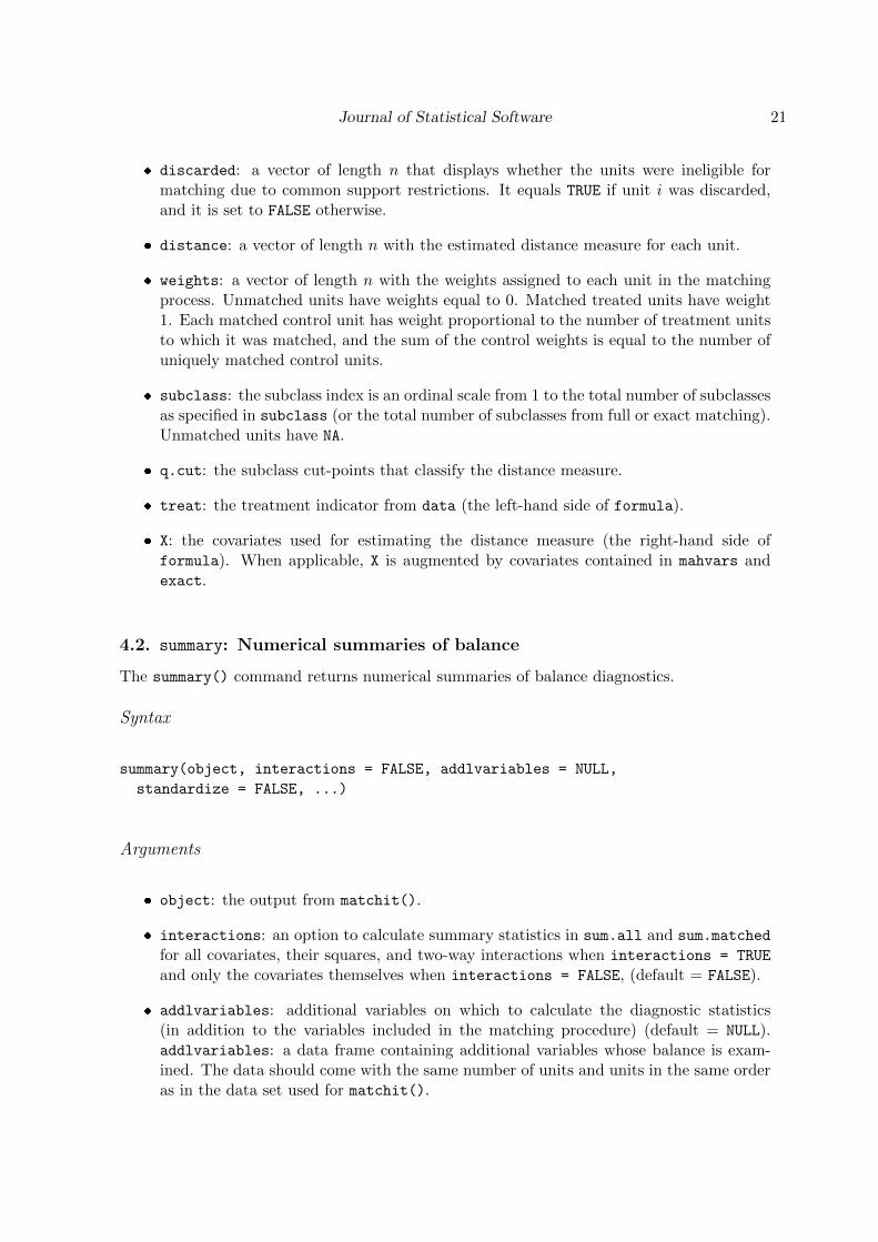
� discarded: a vector of length n that displays whether the units were ineligible formatching due to common support restrictions. It equals TRUE if unit i was discarded,and it is set to FALSE otherwise.

� distance: a vector of length n with the estimated distance measure for each unit.

� weights: a vector of length n with the weights assigned to each unit in the matchingprocess. Unmatched units have weights equal to 0. Matched treated units have weight1. Each matched control unit has weight proportional to the number of treatment unitsto which it was matched, and the sum of the control weights is equal to the number ofuniquely matched control units.

� subclass: the subclass index is an ordinal scale from 1 to the total number of subclassesas specified in subclass (or the total number of subclasses from full or exact matching).Unmatched units have NA.

� q.cut: the subclass cut-points that classify the distance measure.

� treat: the treatment indicator from data (the left-hand side of formula).

� X: the covariates used for estimating the distance measure (the right-hand side offormula). When applicable, X is augmented by covariates contained in mahvars andexact.

4.2. summary: Numerical summaries of balance

The summary() command returns numerical summaries of balance diagnostics.

Syntax

summary(object, interactions = FALSE, addlvariables = NULL,

standardize = FALSE, ...)

Arguments

� object: the output from matchit().

� interactions: an option to calculate summary statistics in sum.all and sum.matched

for all covariates, their squares, and two-way interactions when interactions = TRUE

and only the covariates themselves when interactions = FALSE, (default = FALSE).

� addlvariables: additional variables on which to calculate the diagnostic statistics(in addition to the variables included in the matching procedure) (default = NULL).addlvariables: a data frame containing additional variables whose balance is exam-ined. The data should come with the same number of units and units in the same orderas in the data set used for matchit().


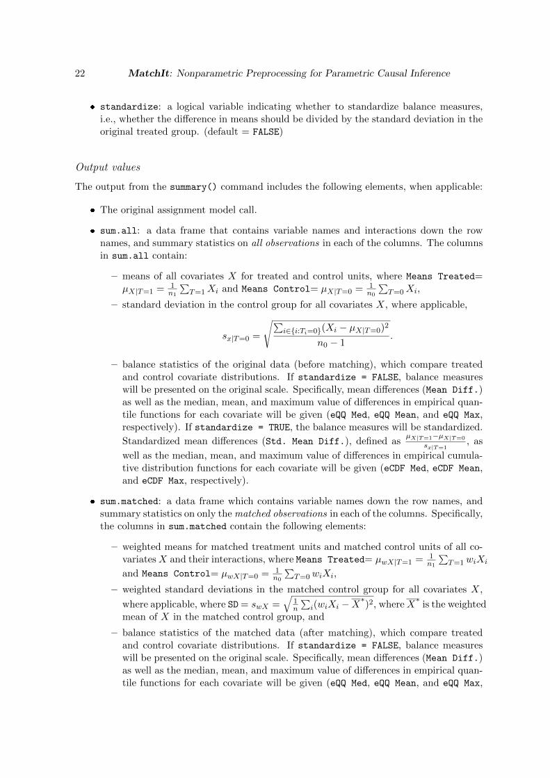
� standardize: a logical variable indicating whether to standardize balance measures,i.e., whether the difference in means should be divided by the standard deviation in theoriginal treated group. (default = FALSE)

Output values

The output from the summary() command includes the following elements, when applicable:

� The original assignment model call.

� sum.all: a data frame that contains variable names and interactions down the rownames, and summary statistics on all observations in each of the columns. The columnsin sum.all contain:

– means of all covariates X for treated and control units, where Means Treated=µX|T=1 = 1

n1

∑T=1Xi and Means Control= µX|T=0 = 1

n0

∑T=0Xi,

– standard deviation in the control group for all covariates X, where applicable,

sx|T=0 =

√∑i∈{i:Ti=0}(Xi − µX|T=0)2

n0 − 1.

– balance statistics of the original data (before matching), which compare treatedand control covariate distributions. If standardize = FALSE, balance measureswill be presented on the original scale. Specifically, mean differences (Mean Diff.)as well as the median, mean, and maximum value of differences in empirical quan-tile functions for each covariate will be given (eQQ Med, eQQ Mean, and eQQ Max,respectively). If standardize = TRUE, the balance measures will be standardized.

Standardized mean differences (Std. Mean Diff.), defined asµX|T=1−µX|T=0

sx|T=1, as

well as the median, mean, and maximum value of differences in empirical cumula-tive distribution functions for each covariate will be given (eCDF Med, eCDF Mean,and eCDF Max, respectively).

� sum.matched: a data frame which contains variable names down the row names, andsummary statistics on only the matched observations in each of the columns. Specifically,the columns in sum.matched contain the following elements:

– weighted means for matched treatment units and matched control units of all co-variatesX and their interactions, where Means Treated= µwX|T=1 = 1

n1

∑T=1wiXi

and Means Control= µwX|T=0 = 1n0

∑T=0wiXi,

– weighted standard deviations in the matched control group for all covariates X,

where applicable, where SD = swX =√

1n

∑i(wiXi −X

∗)2, whereX

∗is the weighted

mean of X in the matched control group, and

– balance statistics of the matched data (after matching), which compare treatedand control covariate distributions. If standardize = FALSE, balance measureswill be presented on the original scale. Specifically, mean differences (Mean Diff.)as well as the median, mean, and maximum value of differences in empirical quan-tile functions for each covariate will be given (eQQ Med, eQQ Mean, and eQQ Max,


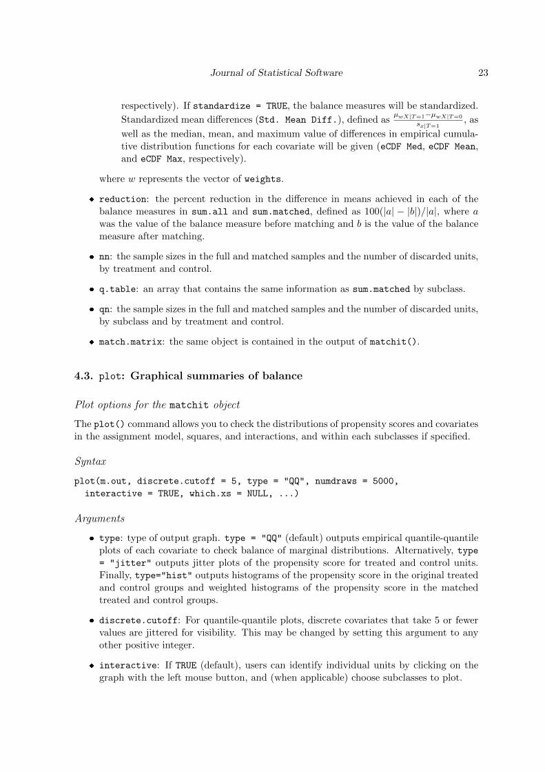
respectively). If standardize = TRUE, the balance measures will be standardized.

Standardized mean differences (Std. Mean Diff.), defined asµwX|T=1−µwX|T=0

sx|T=1, as

well as the median, mean, and maximum value of differences in empirical cumula-tive distribution functions for each covariate will be given (eCDF Med, eCDF Mean,and eCDF Max, respectively).

where w represents the vector of weights.

� reduction: the percent reduction in the difference in means achieved in each of thebalance measures in sum.all and sum.matched, defined as 100(|a| − |b|)/|a|, where awas the value of the balance measure before matching and b is the value of the balancemeasure after matching.

� nn: the sample sizes in the full and matched samples and the number of discarded units,by treatment and control.

� q.table: an array that contains the same information as sum.matched by subclass.

� qn: the sample sizes in the full and matched samples and the number of discarded units,by subclass and by treatment and control.

� match.matrix: the same object is contained in the output of matchit().

4.3. plot: Graphical summaries of balance

Plot options for the matchit object

The plot() command allows you to check the distributions of propensity scores and covariatesin the assignment model, squares, and interactions, and within each subclasses if specified.

Syntax

plot(m.out, discrete.cutoff = 5, type = "QQ", numdraws = 5000,

interactive = TRUE, which.xs = NULL, ...)

Arguments

� type: type of output graph. type = "QQ" (default) outputs empirical quantile-quantileplots of each covariate to check balance of marginal distributions. Alternatively, type= "jitter" outputs jitter plots of the propensity score for treated and control units.Finally, type="hist" outputs histograms of the propensity score in the original treatedand control groups and weighted histograms of the propensity score in the matchedtreated and control groups.

� discrete.cutoff: For quantile-quantile plots, discrete covariates that take 5 or fewervalues are jittered for visibility. This may be changed by setting this argument to anyother positive integer.

� interactive: If TRUE (default), users can identify individual units by clicking on thegraph with the left mouse button, and (when applicable) choose subclasses to plot.


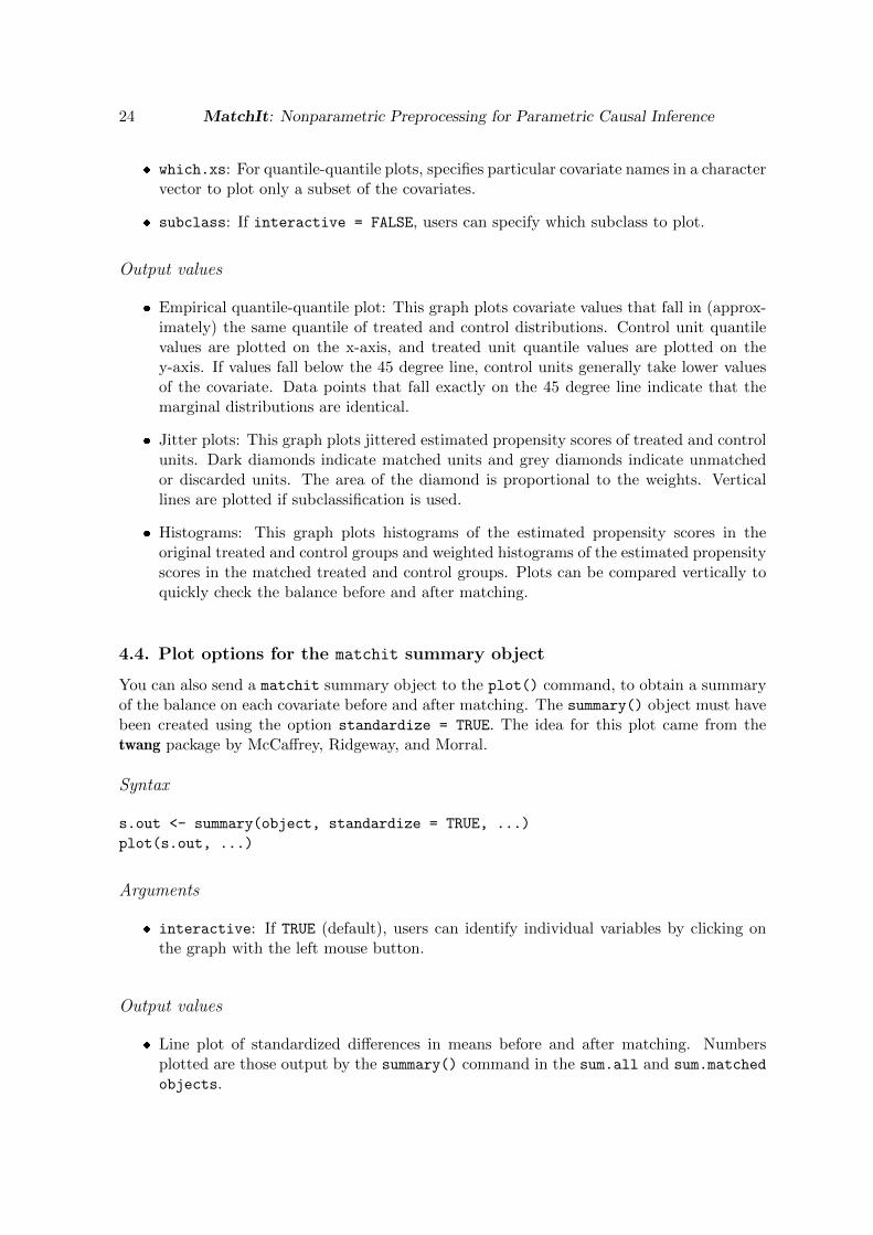
� which.xs: For quantile-quantile plots, specifies particular covariate names in a charactervector to plot only a subset of the covariates.

� subclass: If interactive = FALSE, users can specify which subclass to plot.

Output values

� Empirical quantile-quantile plot: This graph plots covariate values that fall in (approx-imately) the same quantile of treated and control distributions. Control unit quantilevalues are plotted on the x-axis, and treated unit quantile values are plotted on they-axis. If values fall below the 45 degree line, control units generally take lower valuesof the covariate. Data points that fall exactly on the 45 degree line indicate that themarginal distributions are identical.

� Jitter plots: This graph plots jittered estimated propensity scores of treated and controlunits. Dark diamonds indicate matched units and grey diamonds indicate unmatchedor discarded units. The area of the diamond is proportional to the weights. Verticallines are plotted if subclassification is used.

� Histograms: This graph plots histograms of the estimated propensity scores in theoriginal treated and control groups and weighted histograms of the estimated propensityscores in the matched treated and control groups. Plots can be compared vertically toquickly check the balance before and after matching.

4.4. Plot options for the matchit summary object

You can also send a matchit summary object to the plot() command, to obtain a summaryof the balance on each covariate before and after matching. The summary() object must havebeen created using the option standardize = TRUE. The idea for this plot came from thetwang package by McCaffrey, Ridgeway, and Morral.

Syntax

s.out <- summary(object, standardize = TRUE, ...)

plot(s.out, ...)

Arguments

� interactive: If TRUE (default), users can identify individual variables by clicking onthe graph with the left mouse button.

Output values

� Line plot of standardized differences in means before and after matching. Numbersplotted are those output by the summary() command in the sum.all and sum.matched

objects.


4.5. match.data: Extracting the matched data set

Usage

To extract the matched data set for subsequent analyses from the output object (as describedin Section 3.3), we provide the function match.data(). This is used as follows:

m.data <- match.data(object, group = "all", distance = "distance",

weights = "weights", subclass = "subclass")

The output of the function match.data() is the original data frame where additional infor-mation about matching (i.e., distance measure as well as resulting weights and subclasses) isadded, restricted to units that were matched.

4.6. Arguments

match.data() takes the following inputs:

1. object is the output object from matchit(). This is a required input.

2. group specifies for which matched group the user wants to extract the data. Availableoptions are "all" (all matched units), "treat" (matched units in the treatment group),and "control" (matched units in the control group). The default is "all".

3. distance specifies the variable name used to store the distance measure. The defaultis "distance".

4. weights specifies the variable name used to store the resulting weights from matching.The default is "weights". See Section 3.3.2 for more details on the weights.

5. subclass specifies the variable name used to store the subclass indicator. The defaultis "subclass".

4.7. Examples

Here, we present examples for using match.data(). Users can run these commands by typingdemo("match.data") at the R prompt. First, we load the Lalonde data,

data("lalonde")

The next line performs nearest neighbor matching based on the estimated propensity scorefrom the logistic regression,

R> m.out1 <- matchit(treat ~ re74 + re75 + age + educ, data = lalonde,

+ method = "nearest", distance = "logit")

To obtain matched data, type the following command,

R> m.data1 <- match.data(m.out1)


It is easy to summarize the resulting matched data,

R> summary(m.data1)

To obtain matched data for the treatment or control group, specify the option group asfollows,

R> m.data2 <- match.data(m.out1, group = "treat")

R> summary(m.data2)

R> m.data3 <- match.data(m.out1, group = "control")

R> summary(m.data3)

We can also use the function to return unmatched data:

R> unmatched.data <-

+ lalonde[!row.names(lalonde) %in% row.names(match.data(m.out1)), ]

We can also specify different names for the subclass indicator, the weight variable, and theestimated distance measure. The following example first does a subclassification method,obtains the matched data with specified names for those three variables, and then print outthe names of all variables in the resulting matched data.

R> m.out2 <- matchit(treat ~ re74 + re75 + age + educ, data = lalonde,

+ method = "subclass")

R> m.data4 <- match.data(m.out2, subclass = "block", weights = "w",

+ distance = "pscore")

R> names(m.data4)

Acknowledgments

We thank Olivia Lau for helpful suggestions about incorporating MatchIt into Zelig andMichael Donnelly, Allie Dunworth, and Olga Zverovich for research assistance. Many thanksalso for financial support from the National Science Foundation (SES-0550873, SES-0752050),the National Institute of Mental Health and the National Institute on Drug Abuse (MH066247),and the Princeton University Committee on Research in the Humanities and Social Sciences.

References

Abadie A, Imbens GW (2006). “Large Sample Properties of Matching Estimators for AverageTreatment Effects.” Econometrica, 74(1), 235–267.

Dehejia RH, Wahba S (1999). “Causal Effects in Nonexperimental Studies: Re-Evaluatingthe Evaluation of Training Programs.” Journal of the American Statistical Association,94(448), 1053–62.


Diamond A, Sekhon J (2010). “Genetic Matching for Estimating Causal Effects: A GeneralMultivariate Matching Method for Achieving Balance in Observational Studies.” URLhttp://sekhon.berkeley.edu/papers/GenMatch.pdf.

Gu X, Rosenbaum PR (1993). “Comparison of Multivariate Matching Methods: Structures,Distances, and Algorithms.” Journal of Computational and Graphical Statistics, 2(4), 405–420.

Hansen BB (2004). “Full Matching in an Observational Study of Coaching for the SAT.”Journal of the American Statistical Association, 99(467), 609–618.

Ho D, Imai K, King G, Stuart E (2007). “Matching as Nonparametric Preprocessing forReducing Model Dependence in Parametric Causal Inference.” Political Analysis, 15(3),199–236.

Imai K (2005). “Do Get-Out-The-Vote Calls Reduce Turnout? The Importance of StatisticalMethods for Field Experiments.” American Political Science Review, 99(2), 283–300.

Imai K, King G, Lau O (2008a). “Toward a Common Framework for Statistical Analysis andDevelopment.” Journal of Computational and Graphical Statistics, 17(4), 1–22.

Imai K, King G, Lau O (2011). Zelig: Everyone’s Statistical Software. R package version 3.5,URL http://CRAN.R-project.org/package=Zelig.

Imai K, King G, Stuart E (2008b). “Misunderstandings among Experimentalists and Obser-vationalists about Causal Inference.” Journal of the Royal Statistical Society A, 171(2),481–502.

Imai K, van Dyk DA (2004). “Causal Inference with General Treatment Treatment Regimes:Generalizing the Propensity Score.” Journal of the American Statistical Association,99(467), 854–866.

King G, Zeng L (2006). “The Dangers of Extreme Counterfactuals.” Political Analysis, 14(2),131–159.

King G, Zeng L (2007). “When Can History Be Our Guide? The Pitfalls of CounterfactualInference.” International Studies Quarterly, pp. 183–210.

Lalonde R (1986). “Evaluating the Econometric Evaluations of Training Programs.” AmericanEconomic Review, 76(4), 604–620.

R Development Core Team (2011). R: A Language and Environment for Statistical Computing.R Foundation for Statistical Computing, Vienna, Austria. ISBN 3-900051-07-0, URL http:

//www.R-project.org/.

Rosenbaum PR (2002). Observational Studies. 2nd edition. Springer-Verlag, New York.

Sekhon JS (2011). “Multivariate and Propensity Score Matching Software with AutomatedBalance Optimization: The Matching Package for R.” Journal of Statistical Software, 42(7),1–52. URL http://www.jstatsoft.org/v42/i07/.

http://sekhon.berkeley.edu/papers/GenMatch.pdf

http://CRAN.R-project.org/package=Zelig

http://www.R-project.org/

http://www.R-project.org/

http://www.jstatsoft.org/v42/i07/


Affiliation:

Daniel E. HoStanford Law School559 Nathan Abbott WayStanford, CA 94305, United States of AmericaE-mail: [email protected]: http://dho.stanford.edu/Telephone: +1-650-723-9560Fax: +1-650-725-0253

Kosuke ImaiDepartment of PoliticsPrinceton UniversityPrinceton, NJ 08544, United States of AmericaE-mail: [email protected]: http://imai.princeton.edu/Telephone: +1-609-258-6601Fax: +1-609-258-1110

Gary KingDepartment of GovernmentHarvard University1737 Cambridge StreetCambridge, MA 02138, United States of AmericaE-mail: [email protected]: http://gking.harvard.edu/Telephone: +1-617-495-2027Fax: +1-617-812-8581

Elizabeth A. StuartDepartments of Mental Health and BiostatisticsJohns Hopkins Bloomberg School of Public Health624 North Broadway, Room 804Baltimore, MD 21205, United States of AmericaE-mail: [email protected]: http://faculty.jhsph.edu/default.cfm?faculty_id=1792Telephone: +1-410-502-6222Fax: +1-410-955-9088

Journal of Statistical Software http://www.jstatsoft.org/

published by the American Statistical Association http://www.amstat.org/

Volume 42, Issue 8 Submitted: 2006-07-28May 2011 Accepted: 2008-01-17

mailto:[email protected]

http://dho.stanford.edu/


http://imai.princeton.edu/


http://gking.harvard.edu/


http://faculty.jhsph.edu/default.cfm?faculty_id=1792

http://www.jstatsoft.org/

http://www.amstat.org/

MatchIt: Nonparametric Preprocessing for Parametric Causal ... · MatchIt is an R program, and also...

Documents

Transcript of MatchIt: Nonparametric Preprocessing for Parametric Causal ... · MatchIt is an R program, and also...