Matching as Nonparametric Preprocessing for Reducing - Gary King

Matching as Nonparametric Preprocessing forReducing Model Dependence in Parametric

Causal Inference

Daniel E. Ho

Stanford Law School, 559 Nathan Abbott Way, Stanford, CA 94305

e-mail: [email protected]

Kosuke Imai

Department of Politics, Princeton University,

Princeton, NJ 08544


Gary King

Department of Government, Harvard University,

1737 Cambridge Street, Cambridge, MA 02138

e-mail: [email protected] (corresponding author)

Elizabeth A. Stuart

Departments of Mental Health and Biostatistics,

Johns Hopkins Bloomberg School of Public Health,

624 North Broadway, Room 804, Baltimore, MD 21205


Although published works rarely include causal estimates from more than a few model

specifications, authors usually choose the presented estimates from numerous trial runs

readers never see. Given the often large variation in estimates across choices of control

variables, functional forms, and other modeling assumptions, how can researchers ensure

that the few estimates presented are accurate or representative? How do readers know that

publications are not merely demonstrations that it is possible to find a specification that fits

the author’s favorite hypothesis? And how do we evaluate or even define statistical prop-

erties like unbiasedness or mean squared error when no unique model or estimator even

exists? Matching methods, which offer the promise of causal inference with fewer assump-

tions, constitute one possible way forward, but crucial results in this fast-growing method-

ological literature are often grossly misinterpreted. We explain how to avoid these

Authors’ note: Our thanks to Dan Carpenter and Jeff Koch for data; Alberto Abadie, Neal Beck, Sam Cook,Alexis Diamond, Ben Hansen, Guido Imbens, Olivia Lau, Gabe Lenz, Paul Rosenbaum, Don Rubin, and JasSekhon for many helpful comments; and the National Institutes of Aging (P01 AG17625-01), the NationalInstitute of Mental Health (MH066247), the National Science Foundation (SES-0318275, IIS-9874747, SES-0550873), and the Princeton University Committee on Research in the Humanities and Social Sciences forresearch support. Software to implement the methods in this paper is available at http://GKing.Harvard.edu/matchit and a replication data file is available as Ho et al. (2006).

� The Author 2007. Published by Oxford University Press on behalf of the Society for Political Methodology.All rights reserved. For Permissions, please email: [email protected]

199

Advance Access publication January 31, 2007 Political Analysis (2007) 15:199–236doi:10.1093/pan/mpl013

http://GKing.Harvard.edu/matchit

http://GKing.Harvard.edu/matchit

misinterpretations and propose a unified approach that makes it possible for researchers to

preprocess data with matching (such as with the easy-to-use software we offer) and then to

apply the best parametric techniques they would have used anyway. This procedure makes

parametric models produce more accurate and considerably less model-dependent causal

inferences.

1 Introduction

Political science research typically begins by first spending considerable time collecting,correcting, recollecting, merging, and recoding data. When all the data are finally availablein the right format and loaded into one’s favorite statistical package, researchers obtaina causal estimate by running some parametric statistical procedure—linear regression,logit, probit, duration models, structural equation models, count models, etc. This runtypically takes only a few seconds and, according to some textbooks, it would be time towrite up the results. Of course, this never happens. Instead, we do a second run withdifferent control variables, a third with a different functional form, a fourth with a differentmeasure of our key causal variable, one with different sample periods or observationsubsets, and then each of these and others are repeated with slight variations over andover again. Although this usual procedure produces hundreds or thousands of alternativeestimates of our single causal effect, we typically only choose one, and rarely more than5–10, to present in a paper. Yet, we know that our estimates depend on their correspondingmodeling assumptions and that different specifications can yield very different causalinferences.

Most causal effect estimates given in the literature are thus model dependent, at leastto some degree, but at the same time the statistical properties of most estimators usedby political scientists depend on the assumption that we know the single correctmodel. Model dependence combined with likelihood, Bayesian, or other methods thatcondition on a single model, framework, or specification mean that we cannot logicallyeven ask whether an estimator has desirable properties, such as unbiasedness, consistency,efficiency, mean squared error, etc., since a unique estimator must exist before it can beevaluated. The related practical problem for researchers is how to convince readers that wepicked the right specification rather than the one that most supported our favorite hypoth-esis. What does it even mean to choose ‘‘the right’’ parametric model estimates when anychosen model depends on assumptions we cannot verify? When we read a publishedarticle, how do we know whether the causal effect presented is accurate or whether thearticle merely constitutes a demonstration that it is possible to find a specification consis-tent with the author’s prior expectations? King and Zeng (2006) offer methods to detect theproblem of model dependence; we show how to ameliorate it, when possible.

We begin where virtually all causal inference methods based on observational databegin, by making the ignorability (or no omitted variable bias) assumption and condition-ing on the definition of a key causal (or ‘‘treatment’’) variable and a set of variables wechoose to control for. From this common starting point, we offer an easy method ofadjusting for as much of the information in these control variables as possible withoutparametric assumptions. We do this by preprocessing a data set with matching methods sothat the treated group is as similar as possible to the control group. In the preprocessed dataset, the treatment variable is closer to being independent of the background covariates,which renders any subsequent parametric adjustment either irrelevant or less important.

This inferential strategy has three key advantages. First, the approach is easy to usesince researchers need not give up their familiar parametric analysis methods. Instead, they

200 Daniel E. Ho et al.

merely add a simple preprocessing step before the parametric analysis procedures theywould have used anyway (or should have used anyway if they are not already followingbest practices). All of the intuition, diagnostics, uncertainty estimates, and knowledgeabout parametric procedures can then be used as before. Second, by breaking or reducingthe link between the treatment variable and control variables, preprocessing makes esti-mates based on the subsequent parametric analyses far less dependent on modelingchoices and specifications. When the data are of sufficiently high quality so that propermatches are available (in a manner we define below), causal effect estimates do not varymuch even when changing parametric modeling assumptions. Finally, since most of theadjustment for potentially confounding control variables is done nonparametrically, thepotential for bias is greatly reduced compared to parametric analyses based on raw data.Furthermore, in many situations, the same preprocessing also leads to a reduction in thevariance of the estimated causal effects, and so the mean squared error will normally belower too.

In a sense, our recommendations already constitute current best practice since matchingalone is not a method of estimation and always requires some technique after matching tocompute estimates. The problem is that the method most commonly chosen after matchinghas been a simple difference in means without any controls for potential confoundingvariables. We simply point out that, except in the extraordinary case where matching isexact, common parametric procedures have the potential to greatly improve causal infer-ences even after matching.

The fast-growing matching literature is theoretically sophisticated, but, from the pointof view of the practical researcher, it looks like a cacophony of conflicting techniques,practices, conventions, and rules of thumb. Confusion reigns over computing standarderrors and confidence intervals due to apparently contradictory differences stemming fromalternative nonparametric and parametric perspectives. Many theoretical results do notapply to practical applications unless unknown theoretical quantities or specificationsare somehow divined. Perhaps as a consequence, some of the most important theoreticalresults are routinely misinterpreted in applied research and even in some theoreticalstatistical work. Coherent guidelines for practice are often conflicting, absent, or mis-understood. We try to clarify the key misunderstandings in this literature and to presenta coherent unified perspective for applied research.1

Our approach is similar in spirit to, or a generalization of the ideas in, Cochran andRubin (1973), Rubin (1973, 1979), Rosenbaum and Rubin (1984), Rubin and Thomas(2000), and Imai and van Dyk (2004) who each recommend matching followed by a dif-ferent form of parametric adjustment, as well as strategies used in applied research prob-lems by Rosenbaum (1986) and others, as discussed in Glazerman, Levy, and Myers(2003).2 To our knowledge, the present paper is the first to propose and work out the

1Although matching methods now comprise a substantial fraction of the empirical work in observational studiesin some disciplines, such as epidemiology and medicine, the diversity of substantive applications and theconflicting methodological languages used to describe the same underlying concepts have limited the spreadof these powerful techniques to much of the social sciences. However, the misunderstandings we discuss here areno less prevalent in these other areas.2It is also similar to Heckman, Ichimura, and Todd (1998) who developed forms of matching combined withsemiparametric (kernel weighting) analyses, as well as to the parametric bias adjustment for one form ofmatching by Abadie and Imbens (2006b), except that, to avoid inducing new biases, we recommend below thatmatching be evaluated prior to examining the dependent variable, which is not the case with these latterapproaches as generally implemented. Our idea is also similar in spirit to methods in other areas that preprocessdata so that subsequent analyses can be improved without modifying existing techniques, such as multipleimputation (Rubin 1987; King et al. 2001) and outlier and feature detection (Bishop 1995, chap. 8).

Matching as Nonparametric Preprocessing for Reducing Model Dependence 201

conditions for matching as a general method of nonparametric preprocessing, suitable forimproving any parametric method.

Our general preprocessing strategy also made it possible for us to write easy-to-usesoftware that implements all the ideas discussed in this paper and incorporates mostexisting approaches described in the literature. The program, called MatchIt, is availableas an open source and free R package at http://gking.harvard.edu/matchit (see Appendix);MatchIt also works seamlessly with the general purpose R statistics package called Zelig(Imai, King, and Lau 2006).

Other approaches to reducing model dependence include weighting (Hirano, Imbens,and Ridder 2003; Robins and Rotnitzky forthcoming), nonparametric techniques, robustestimation, and fitting checks for parametric models. Although when used properly each ofthese approaches can reduce model dependence, matching may be simpler to use andunderstand and would work as we suggest here to improve all the parametric modelsnow used for making causal inferences in the social sciences. More importantly, sincethese alternative approaches also involve specification or modeling decisions, preprocess-ing via matching works well in combination with these approaches too, and so they shouldnot be considered competitors. Other seemingly possible alternatives, such as Bayesianmodel averaging (Hoeting et al. 1999; Imai and King 2004) and cross-validation (Blackand Smith 2004), are useful for predictive inference but not directly applicable in thecontext of causal inference.

2 Definition of Causal Effects

The notation, ideas, and running example in this section parallel that in King, Keohane,and Verba (1994, sec. 3.1.1), but key aspects of the ideas originate with many others,especially Neyman (1923), Fisher (1935), Cox (1958), Rubin (1974), and Holland (1986)in statistics; Roy (1951) and Quandt (1972) in econometrics; and Lewis (1973) in philos-ophy. The most important idea in this section is that a causal effect is a theoretical quantity,defined independently of any empirical method that might be used to estimate it fromreal data.

Our running example in this section is estimating the electoral advantage of incum-bency for Democrats in the U.S. House of Representatives. In most of the methodologicalliterature on causal inference, researchers simplify the exposition by considering onlya single dichotomous causal (or treatment) variable. We do the same and label it Ti, whichtakes a value of 1 if congressional district i ði5 1; . . . ; nÞ receives the treatment and 0 if i isuntreated (the ‘‘control condition’’). In our example, the treatment is whether the Demo-cratic incumbent receives the party’s nomination in district i.

The observed outcome (or ‘‘dependent’’) variable is yi, which in our case is the Dem-ocratic proportion of the two-party vote in district i. Finally, each district i has a variety ofcharacteristics determined prior to the incumbent’s decision to run for election and theparty’s decision to renominate the incumbent, some of which we measure and collect ina vector denoted Xi. Whether preprocessing or not, variables that are even in part a con-sequence of the treatment variable should never be controlled for when estimating a causaleffect (see Cox 1958, sec. 4.2; Rosenbaum 1984; Rosenbaum 2002, 73–4). This is ofcourse a critical point since controlling for the consequences of a causal variable canseverely bias a causal inference. For example, controlling for aggregate voting intentionsthe day before the election would obviously control away, and thus bias, the estimatedincumbency effect. This ‘‘posttreatment bias’’ problem is far too common in many areas ofpolitical science (King and Zeng 2007).


http://gking.harvard.edu/matchit

To clarify our inferential goals, we begin by defining the ‘‘fixed causal effect,’’ which isthe simplest in-sample definition available, in that it is the closest to the data. We thengeneralize the definition to include features of random causal effects that are useful forunderstanding connections between nonparametric preprocessing and parametric models,define causal effects of interest at the population level, and discuss multiple and nonbinarytreatments.

2.1 Fixed Causal Effects

Because of pretreatment differences among the districts (both measured, Xi, and unmea-sured), the causal effect may also differ across the districts. We therefore define the casualeffect at the district (i.e., observation) level.

A causal effect is a function of potential outcomes: let yi(1) [ yi(Ti 5 1) be the vote wewould observe in district i in say the 2008 election if in fact the Democratic incumbentreceives his or her party’s nomination (i.e., Ti 5 1), and let yi(0) [ yi(Ti 5 0) be the votewe would observe if the Democratic Party nominates a nonincumbent (i.e., Ti 5 0). (Eachof the potential vote outcomes in district i is thus a function of the incumbency status in thesame district, Ti, and not a function of candidates in other districts.) The use of parenthesesin this notation denotes that the outcome is potential, and so not necessarily observed, andthat it depends on the value of the variable in parentheses. Since these are potential out-comes, their values remain the same regardless of whether the treatment is in fact appliedin district i or not.

The difference between the two potential outcomes defines the fixed (or unit specific)causal effect

Fixed causal effect for unit i[ yið1Þ � yið0Þ: ð1Þ

(This quantity is an unobserved realization of a random variable to be defined below.)Since the Democratic Party will either nominate (Ti 5 1) or not nominate (Ti 5 0) anincumbent to run in district i, one of these potential outcomes is always a counterfactualand thus never observed. This is known as the ‘‘fundamental problem of causal inference’’(Holland 1986).

2.2 Random Causal Effects

Now, imagine that the potential outcomes in equation (1) are realizations of correspondingrandom variables (for which we use the corresponding capital letters). This produces therandom causal effect

Random causal effect for unit i[Yið1Þ � Yið0Þ; ð2Þ

features of which constitute alternative quantities of interest. For example, our secondcausal effect is the mean causal effect, which is the average over repeated hypotheticaldraws of the random causal effect

Mean causal effect[Eðrandom causal effectÞ ð3Þ

5E½Yið1Þ � Yið0Þ�5l1 � l0;

ð4Þ

where l1 [ E[Yi(1)] and l0 [ E[Yi(0)].


2.3 Average Quantities of Interest

In most applications, estimating the treatment effect for each observation is unnecessary;instead, the goal is to estimate the average effect over all observations, for some subset ofobservations or for a particular population. This leads to several choices for quantities ofinterest, each of which is defined for either fixed (in-sample) or population causal effects.We focus on in-sample effects—that is, based on quantities of interest for all or a subset ofunits in our data—since they are closer to the data than effects for averages of specifiedpopulations or population subgroups. However, even for survey researchers and othersinterested in population quantities, the practical difference between population and in-sample estimators is not normally important since a good estimator for one is ‘‘automat-ically a good estimator for the other’’ (Imbens 2004, 6).

Among in-sample effects, we consider two choices. The first is the average treatmenteffect or ATE

ATE[1

n

Xn

i51

E½Yið1Þ � Yið0Þ j Xi�

51

n

Xn

i51

l1ðXiÞ � l0ðXiÞ;ð5Þ

where l0ðXiÞ[E½Yið0ÞjXi� and l1ðXiÞ[E½Yið1ÞjXi�. This quantity is the mean causaleffect for a unit whose characteristics are represented by Xi, averaged over all units (sothat the expectation operator in the first-line averages over the random causal effects foreach unit with the values of the pretreatment variable equal to Xi, and the summation over iin both lines refers to the observed sample).

Often, of more interest substantively is the average treatment effect on the treated orATT

ATT[1Pn

i51 Ti

Xn

i51

TiE½Yið1Þ � Yið0Þ j Xi�

51Pn

i51 Ti

Xn

i51

Ti½l1ðXiÞ � l0ðXiÞ�:ð6Þ

In our example, this is the average causal effect in districts in which the Democratic Partynominated the incumbent member of the House. From one perspective, we might want toknow this treatment effect on the treated (the ATT) since obviously this is the group ofdistricts where the treatment was applied. In other words, the ATT is the effect of thetreatment actually applied. Medical studies typically use the ATT as the designated quan-tity of interest because they often only care about the causal effect of drugs for patients thatreceive or would receive the drugs. For another example, in job training programs, we arenot normally interested in assigning employed people to have this training (Heckman,Ichimura, and Todd 1998). In the social sciences, the ATE is often a reasonable choice, asis the ATT. In our example, we might be interested not only in the effect of incumbencywhen the incumbent is nominated, but we can also imagine what might have happened ifan incumbent were nominated in a district in which he or she did not actually receive thenomination. In this paper, we usually focus on ATT as the quantity of interest when it isconceptually or algebraically simpler, but we also show how to compute the ATE. If causaleffects are constant over i, then the ATT and the ATE are identical.


The ATE and ATT defined above are each in-sample, unconditional estimates. Alter-native quantities of interest are defined by making the choice of unconditional versusconditional and in-sample versus population quantities. In contrast to the unconditionalquantities above, conditional ATE and ATT quantities get even closer to the data byconditioning each on yi. The result is that Yi(1) and Yi(0) in the expressions above arereplaced by yi(1) and yi(0), for each i. Then for each i, only one of the counterfactualoutcomes, yi(1) or yi(0), is estimated and the other is set to the observed yi. These condi-tional, in-sample ATE and ATT quantities are reasonable alternatives that we often use.

Similarly, to change from in-sample quantities in the expressions above to the popula-tion ATE, we average it over (i.e., weight by) the population distribution of X; for the ATT,we average over the conditional distribution of X given T 5 1. Point estimates for thepopulation and sample are normally identical, although the variances for the populationestimates are usually larger.

2.4 Nonbinary and Multiple Treatments

Projects with a causal variable that has more than two categories or is continuous or mixedcan dichotomize (perhaps in several alternative ways) or use more complicated methodsdesigned especially for these variables (Imai and van Dyk 2004). Those with more thanone causal variable of interest can follow all the advice herein for one variable at a time,which would involve matching separately for each and working hard to avoid posttreat-ment bias in the process. We stick to a single binary treatment here since it greatlysimplifies the exposition and improves intuition even for those who will ultimately usemore sophisticated treatments.

3 Assumptions and Data Collection Mechanisms

We now describe the assumptions necessary for making causal inferences in experimentaland observational research. Some version of these assumptions, or some way to deal withthe information in them, is necessary no matter what statistical methods are used forestimation. Any specific statistical method chosen will make additional assumptions,but the ones discussed here affect essentially all methods.

3.1 Experimental Research

Although classical randomized experiments are only rarely conducted in political science,they remain a useful ideal type for understanding other research designs. Indeed, thepreprocessing procedures we recommend alter the data to make them more like whatwe would have seen if an experiment had been conducted.

Valid and relatively straightforward causal inferences can be achieved via classicalrandomized experiments. Such experiments have three critical features: (1) random se-lection of units to be observed from a given population, (2) random assignment of valuesof the treatment to each observed unit,3 and (3) large n (sample size).

Feature (1) avoids selection bias by identifying a given population and guaranteeingthat the probability of selection from this population is related to the potential outcomesonly by random chance. Combining Feature (1) with the large n from Feature (3) guar-antees that the chance that something will go wrong is vanishingly small.

3Below, we assume a classical randomized experiment with simple random assignment rather than randomassignment based on some pretreatment covariates. If treatment assignment depends on observed values ofthe covariates, those covariates should be taken into account in subsequent analyses.


Random assignment in Feature (2) guarantees the absence of omitted variable bias evenwithout any control variables included. To see this, recall that under the usual econometricconditions for omitted variable bias, a variable Xi must be controlled for if it is causallyprior to Ti, empirically related to Ti, and affects Yi conditional on Ti. If instead one or moreof the three conditions do not hold, then Xi may be omitted without any resulting bias(although the variance may increase). Random assignment guarantees that Ti is indepen-dent of any Xi, whether measured or not, except by random chance. Moreover, the largen in Feature (3) guarantees that this chance is vanishingly small.

Classical randomized experiments are a true ideal type, particularly in relation to mostsocial science research, which almost always fails to meet at least one of the three features.Even most social science laboratory experiments have random assignment but no randomselection and often a small n. Traditional survey research has what is intended to berandom selection (although with dramatically increasing nonresponse rates and cell phoneusage, this is a less plausible claim) and certainly has a large n, but random assignment,except when the treatment involves the wording of survey questions, is usually impossible.

3.2 Observational Research

We define observational data collection mechanisms as any process generating data thatdoes not meet all three features of a classical randomized experiment. Scholars trying touse the experimental paradigm attempt to design research to meet all three features dis-cussed in the previous section. Researchers analyzing observational data are instead forcedto make assumptions that, if correct, help them avoid various threats to the validity of theircausal inferences.4

In this paper, we assume data are selected in a manner that does not generate selectionbias. Observations need not be selected at random, as in an experiment, but the probabilityof selection must not depend on potential outcomes. This can be satisfied by carefullyconsidering and controlling for the sample selection process (as in case-control designs) orby changing the quantity of interest to be that reflected by the sample. However it is done,avoiding selection bias is the subject of a great deal of concern and study in a large varietyof methodological and substantive literatures. We mention it here to emphasize that all thewell-known concerns about selecting on the dependent variable should remain a concernto researchers even when adopting our approach of preprocessing data via nonparametricmatching procedures.

We also assume that researchers analyzing observational data have sufficient in-formation in their measured pretreatment control variables Xi so that it is possible viasome method to make valid causal inferences. This is known in political methodologyand econometrics as the absence of ‘‘omitted variable bias,’’ so that Xi must include allvariables that are causally prior to Ti, associated with Ti, and affect Yi conditional onTi (Goldberger 1991; King, Keohane, and Verba 1994), or ‘‘selection on observables’’(Heckman and Robb 1985). In statistics, this same condition is known as ‘‘ignorability,’’which means that Ti and the unobserved potential outcomes are independent after condi-tioning on Xi and the observed potential outcomes, and so we can literally ignore allunobserved variables (Rubin 1978). In biostatistics, it is known as the absence of ‘‘un-measured confounding,’’ and in several fields it is known as ‘‘conditional independence.’’Whatever the name, it is a strong condition, but it is one about which social scientists are

4Our definition of ‘‘observational data’’ is more expansive than some. In some fields, only deviations from randomassignment would be called observational. Our definition emphasizes the necessity of assumptions in generalrather than any ones in particular.


deeply knowledgeable and it is the central methodological concern of many substantivescholarly articles. We emphasize this assumption to make clear that our procedures containno magic: They do not help us control for variables that are not measured.

In the context of the no selection or omitted variable bias assumptions, we haveimplicitly made three others that are worth additional emphasis here. First, the pretreat-ment covariates Xi are truly pretreatment and are thus not consequences of Ti. Second, weassume the independence of units, which is the equivalent of assuming the absence of timeseries or spatial autocorrelation across units (or in other words that the two potentialoutcomes for observation i and the treatment for observation j are independent, for alli 6¼ j). We have also assumed that the treatment administered to each unit is the same. Thisassumption would be violated in our example if incumbency status meant somethingdifferent across districts.5

Satisfying the assumptions discussed in this section still leaves many other assumptionsto be made when choosing a specific statistical inference method. We now focus on thispoint in the context of commonly used parametric methods.

4 Parametric Analysis Methods

Researchers willing to assume that a particular parametric model (up to some unknownparameters) generated their data should specify and directly estimate this model. Prepro-cessing data with matching procedures will not help in this situation. Of course, fewresearchers with observational data sets have this kind of knowledge, and as a result somechoices need to be made among the range of possible parametric models. The dilemma isthat although researchers using parametric methods do not know the true parametricmodel, they must proceed as if they do.

We begin by specifying a single but general parametric model that characterizes therange of models that researchers might choose from. The special cases of this modelinclude almost all parametric models that have been used in the social sciences. First,define the chosen stochastic component for the model as YijTi;Xi ; pðlTiðXiÞ; hÞ for prob-ability density pð�Þ, mean lTiðXiÞ; and vector of ancillary parameters h. Then, denote thesystematic component as lTiðXiÞ[E½YijTi;Xi�5 gðaþ Tibþ XicÞ for some specifiedfunctional form gð�Þ and with intercept a and coefficients b and c. The ancillary param-eters may also be specified to vary over observations as a function of Xi or other covariates.This framework includes all generalized linear models (McCullagh and Nelder 1989), aswell as many others. For example, if pð�Þ is normal and g(c)5 c, we have linear regression;if pð�Þ is Bernoulli and g(c) 5 1/(1 þ e�c), the model reduces to a logistic regression.

We define the ATT in equation (6) under this model by substituting in the definitionsof the potential outcomes from the systematic component, with Ti taking on values 1 and 0,respectively

l1ðXiÞ[E½Yið1Þ j Ti 5 1; Xi�5 gðaþ bþ XicÞ;l0ðXiÞ[E½Yið0Þ j Ti 5 0; Xi�5 gðaþ XicÞ:

ð7Þ

We can produce estimates of these quantities by assuming independence over observationsand forming a likelihood function

5These last two assumptions are sometimes known as the ‘‘stable unit treatment value assumption’’ or SUTVA(Rubin 1974).


Lða; b; c; h jY ;T ;XÞ5Yn

i51

pðYi j gðaþ Tibþ XicÞ; hÞ; ð8Þ

the maximum of which gives parameter estimates, or via Bayesian or other inferentialmethods.

We now turn to the difficulties in making causal inferences from experimental versusobservational data under this general model and conclude this section with an illustrationand formal definition of model dependence.

4.1 Experimental Data

In experimental data, random assignment guarantees (among other things) that Ti and(any observed or unobserved) Xi are independent. In this situation, Xi cannot be a con-founding factor when estimating the effect of Ti, and we drop Xi and replace equation (7)with

E½Yið1Þ j Ti 5 1�[ l1 5 gðaþ bÞ;E½Yið0Þ j Ti 5 0�[ l0 5 gðaÞ

ð9Þ

and the ATT in equation (6) with

ATT5 gðaþ bÞ � gðaÞ; ð10Þ

which importantly no longer has a summation sign over i.The systematic components in equation (9) are now scalar constants for all i. This is

a key result since the functional form gð�Þ no longer models a high-dimensional spacerepresenting how the mean varies over i as a function of all the variables in Xi but insteadnow merely amounts to a simple scalar reparameterization. The fact that gð�Þ is nowa scalar is central: Since maximum likelihood is invariant to reparameterization—mean-ing, for example, that the maximum likelihood estimate (MLE) of a is the same as thepositive square root of the MLE of a2 (King 1989, 75–6)—we get the same estimate of theexpected potential outcomes no matter how gð�Þ is defined.6 When l0 and l1 are a functionof Xi, the choice of gð�Þ is a difficult substantive decision typically requiring more knowl-edge than is available. In contrast, in experimental data, because we can now drop Xi, thechoice of gð�Þ reduces to an easy computational issue with no substantive import. More-over, given any chosen stochastic component, this result holds for a wide range of para-metric models, including all the special cases of the general model given above.

Since the specific maximum likelihood estimator of the population mean for manycommon probability densities is merely the sample mean, the analysis of classical ran-domized experiments typically comes down to taking the difference in the sample meansof Yi for the treatment and control groups. But even if one chooses to run a parametricmodel (for reasons of efficiency, conducting conditional inferences, or because of knowl-edge of the functional form), the absence of model dependence means that the choice fora functional form will not matter: The results will be almost the same no matter whatchoice one makes for the functional form.

6To rule out degenerate cases such as g(a) 5 8, we require that the image of gð�Þ and the range of the potentialoutcomes be the same.


4.2 Observational Data

In experiments, random assignment breaks the link between Ti and Xi, eliminatingthe problem of model dependence. When analyzing observational data with parametricmethods, we are not so fortunate. We cannot reduce equation (7) to equation (9) and soare left having to model the full functional relationship that connects the mean as itvaries as a function of Ti and Xi over observations. Since Xi is typically multidimen-sional, this is a surprisingly difficult task with rather severe consequences for researchpractice.

The problem is the curse of dimensionality and the consequence in practice is modeldependence. We begin with the former and for simplicity suppose that we have a contin-uous dependent variable and one 10-category explanatory variable, and our goal is to uselinear regression to estimate the functional relationship without actually making functionalform assumptions. To do this, we represent the 10 categories with 10 parameters (aconstant and nine dummy variables or equivalently 10 mean indicator variables). Incontrast, the usual approach to estimation is to assume linearity by directly includingthe 10-category variable. This enables us to enter not 10 indicator variables, but ratheronly a constant term and one slope coefficient. How do we get from 10 parameters to onlytwo? Pure assumption. If we have some sense that the relationship is indeed linear or closeto linear, this is a good use of external information to reduce the number of parameters thatmust be estimated. If not, then we still have the best linear approximation to the condi-tional expectation function, but the relationship we estimate can be far off. If we arerunning this regression for the purpose of estimating a causal effect, then the treatmentvariable is also in the regression, and its coefficient can be biased to any degree if thefunctional relationship with the control variables is misspecified.

This problem quickly becomes more serious as the number of explanatory variablesincreases. For example, estimation without functional form assumptions with two 10-category explanatory variables would require not 20 parameters but 100. In this case,the usual approach would include a constant term and two slope coefficients, reducing100 parameters to three by pure assumption. And with multiple explanatory variables,claims about external knowledge constraining the functional form much become dubious.In this example, by what theory would we know that 97 parameters, representing everyform of nonlinearity and interaction, should be set to exactly zero? Including a linearinteraction would not help much since it would merely add one more parameter to esti-mate, and so we would still need to make assumptions about the remaining 96 parameters.

Estimating rather than making assumptions about all these extra parameters is obvi-ously not possible under the standard regression approach since social science data sets donot come with anywhere near enough observations. We cannot avoid the problem withnonlinear or nonnormal statistical models since these pose the same curse of dimension-ality as linear regression. The assumption of ignorability, which enables us to make thepositivist assumption that we have measured and observed all necessary variables, isinsufficient.

Instead, we are led to the inescapable conclusion that, in parametric causal inference ofobservational data, many assumptions about many parameters are frequently necessary,and only rarely do we have sufficient external information to make these assumptionsbased on genuine knowledge. The frequent, unavoidable consequence is high levels ofmodel dependence, with no good reason to choose one set of assumptions over another.Residual and other diagnostics will uncover some forms of misspecification, but the curseof dimensionality prevents any simple parametric solution to the problem.


4.3 Model Dependence in Observational Data

We first illustrate the problem of sensitivity to model specification and then give a moreformal definition of model dependence. The left graph of Figure 1 plots artificial data foroutcome Yi on the vertical axis and a pretreatment covariate Xi on the horizontal axis (wediscuss the right graph in Section 5.2). This data set was designed to illustrate the problem;in real examples, aspects of the problem we portray here often appear, but they may bemore difficult to see given the simultaneous presence of other methodological problems.In addition, although a good data analyst could easily identify outliers in this one-dimensional case, doing so is harder in the usual situation with many covariates. In thisfigure, each data point is plotted as a ‘‘T’’ for treated units (Ti 5 1) and ‘‘C’’ for controlunits (Ti 5 0). We then fit two regressions to these data. The first is a linear regression ofYi on a constant, Ti, and Xi: E[Yi | Ti, Xi] 5 a þ Tib þ Xic. The fitted values for thisregression are portrayed in two parallel solid lines, the dark solid line for the treated group,E[Yi | Ti 5 1, Xi]5 aþ bþ Xic, and the gray solid line for the controls, E[Yi | Ti 5 0, Xi]5a þ Xic. The positive vertical distance between the two straight lines is this parametricmodel’s causal effect estimate.

Model dependence is easy to see by also fitting a quadratic model to the same data,which merely involves adding an X2

i term to the original linear regression. Fitted values forthe quadratic regression appear as dashed curves in the same left graph, again gray for thecontrols and solid black for the treated. Clearly, these fit the same data markedly differ-ently from the original regression. Not only is the overall shape completely different, but

Fig. 1 Model sensitivity of ATE estimates for imbalanced raw and balanced matched data. Thisfigure presents an artificial data set of treated units represented by ‘‘T’’ and control units representedby ‘‘C.’’ The vertical axis plots Yi and the horizontal axis plots Xi. The panels depict estimates of theATE for a linear and quadratic specification, represented by the difference between parallel lines andparabolas, respectively. Dark lines are fitted to the treated points and gray to the controls. In the rawdata, plotted in the left panel, some of the control units are far outside the range of the treated units,and these outlying control units are influential in the parametric models. In the matched data, plottedin the right panel, treated units are matched with control units that are close in Xi (gray units arediscarded), and as a result treatment effect estimates are similar regardless of model specification.The two linear and two quadratic lines also appear on the right graph (on top of one another),truncated to the location of the matched data.


the causal effect has now switched signs, which can be seen because the gray solid line isbelow the dark solid line, whereas the gray dashed curve is above the dark dashed curve.

Ultimately, these two models estimate the causal effect by the average vertical distancebetween the C’s and T’s. They differ only in how they compute this average. In this case,the linear model estimates a causal effect of 0.05, whereas the quadratic model estimatesa causal effect of �0.04, and of course other models would yield other estimates. A keyproblem that generates this model dependence is the presence of control units far outsidethe range of the treated units. The model estimation thus extrapolates over a range of datathat do not include treated and control units and so is particularly sensitive to the set ofcontrol units that do not look similar to the treated units. These extrapolations make causaleffect estimates exquisitely sensitive to minor modifications in the statistical model (Kingand Zeng 2007).

Some researchers surely respond to this diversity of possible models by inadvertentlychoosing specifications that support their favored hypotheses. Current best practice is toportray forthrightly at least some aspects of specification uncertainty in published work bygiving results for multiple specifications and evaluating how model dependent the sub-stantive results are. But researchers of course do not often go very far in portraying thesensitivity of their causal inferences to model specification, and conveying all the sensi-tivity is essentially impossible.

In attempting to develop methods that indicate the degree of model dependence thatcould possibly occur given only a set of explanatory variables, King and Zeng (2006)‘‘define model dependence at point x as the difference, or distance, between the predictedoutcome values from any two plausible alternative models . . . . By ‘plausible’ alternativemodels, we mean models that fit the data reasonably well and, in particular, they fit aboutequally well around either the ‘center’ of the data (such as a multivariate mean or median)or the center of a sufficiently large cluster of data nearest the counterfactual x of interest.’’In our case, the predicted outcome values are predicted potential outcomes, Yi(0) and Yi(1),which in our framework can be modeled separately at the parametric stage and each ofwhich may have issues with model dependence. In practice, of course, additional modeldependence will occur when models are chosen that do not fit the data. The left graph inFigure 1 obviously combines both sources of model dependence.

5 Nonparametric Preprocessing

The goal of matching in general and our specific nonparametric preprocessing approach inparticular is to adjust the data prior to the parametric analysis so that (1) the relationshipbetween Ti and Xi is eliminated or reduced and (2) little bias and inefficiency is induced. Ifwe are able to adjust the data so that Ti and Xi are completely unrelated (which makes thecontrol and treatment groups identical with respect to Xi), we will have moved a good dealof the way from Section 4.2 to Section 4.1. An assumption of ignorability is still necessary,but we would no longer need to model the full parametric relationship between the de-pendent variable and the multidimensional Xi. This also eliminates an important source ofmodel dependence in the resulting parametric analysis stemming from the functional formspecification and the curse of dimensionality. For data sets where preprocessing reducesthe extent of the relationship between Ti and Xi, but is unable to make them completelyunrelated, model dependence is not eliminated but will normally be greatly reduced. Ifnonparametric preprocessing results in no reduction of model dependence, then it is likelythat the data have little information to support causal inferences by any method, which ofcourse would also be useful information.


5.1 The Immediate Goal of Preprocessing

How can we adjust the data without inducing bias in our causal estimates? The key to thisproblem is that the fundamental rule for avoiding selection bias—not selecting on thedependent variable—does not prevent us from selecting observations on the explanatoryvariables (Ti or Xi). (Random or other physical assignments that depend on observedcovariates, such as matched pair or randomized block designs, in experiments and strat-ified sampling in surveys are other examples of valid data collection mechanisms thatselect observations given chosen values of the explanatory variables.) We can also select,duplicate, or selectively drop observations from an existing sample without bias, as long aswe do so using a rule that is a function only of Ti and Xi. Our preprocessed data set willtherefore include a selected subset of the observed sample for which Ti and Xi are un-related, meaning that the treatment and control groups have the same background char-acteristics, or in other words that this relationship holds

pðX j T 5 1Þ5 pðX j T 5 0Þ; ð11Þ

where p(�) refers to the observed empirical density of the data, rather than a populationdensity.7 The simplest way to understand how we can satisfy equation (11) by preprocess-ing is via one-to-one exact matching. The idea is to match each treated unit with onecontrol unit for which all the values of Xi are identical. Our preprocessed data set thus is thesame as the original data set with any unmatched control units discarded and thus with Ti

and Xi now independent. If all treated units are matched, this procedure eliminates alldependence on the functional form in the parametric analysis. (If some treated units cannotbe matched, then they either need to be adjusted during parametric modeling, which ofcourse risks extrapolation bias, or dropped, which can change the quantity of interest.) It isalso highly intuitive since it directly parallels an experiment where we find pairs of unitsthat are identical in all observable ways and assign one from each pair to be treated and theother to be a control. Then no matter what effect Xi has on Yi, we can ignore it entirely sinceXi is literally held constant within each pair of units.

Although one-to-one exact matching can eliminate model dependence and any biasfrom incorrect assumptions made during the parametric stage of analysis, it is not the onlyway to break the link between Ti and Xi, since satisfying equation (11) only requires thedistributions to be equivalent. Thus, to be clear, matching does not require pairing ob-servations (indeed, there might have been less confusion if the technique had been called‘‘pruning’’); only the distributions need be matched as closely as possible. Moreover, exactmatching has the disadvantage in many applications of using relatively little of the data.Finding matches is often most severe if Xi is high dimensional (another effect of the curseof dimensionality) or contains continuous variables. The result may then be a preprocesseddata set with very few observations that leads to a parametric analysis with large standarderrors. If this occurs, common practice is to use some form of inexact matching thatbalances as well as possible, which thus effectively sacrifices some bias reduction forthe increased efficiency that comes from having more observations in the preprocesseddata set. In our approach, if we lose some opportunity for bias reduction, we do soonly in the preprocessing stage; the researcher’s second-stage parametric analysis stillhas a chance to eliminate the remaining bias. Details about how to match when exact

7To be more specific, the empirical density is defined as pðxÞ5 #fi 2 f1; 2; . . . ; ng : Xi 5 xg=n; for all x, where#A is the number of elements in the set A. The corresponding denominator n is

Pni51 Ti on the left side andPn

i5 1ð1� TiÞ on the right of equation (11).


one-to-one matching is infeasible appear in our software documentation; common mis-understandings of the theoretical literature on approximate matching appear in Section 6.

A key point about matching as nonparametric preprocessing is that matching is nota method of estimation: obtaining causal effect estimates from matching requires that itbe paired with some analysis method. In the vast majority of applications, the analysismethod has been a simple difference in means between the treatment and control groups.This method certainly makes sense in the case of exact one-to-one matching since mostparametric procedures applied to exactly matched data would give the same estimates.However, with matching that is not exact, using the difference in means estimator is equiv-alent to assuming that any remaining imbalance in the matched sample is strictly unrelatedto the treatment, which we know is false, or has no effect on the outcome, which we have noevidence about before consulting the outcome variable, and we will often have good evi-dence to the contrary in real analyses. Thus, we recommend that scholars make use of theirdecades of experience with parametric models to adjust (i.e., to interpolate or slightlyextrapolate) the matched sample. The adjustment necessary is far less onerous, model de-pendent, and thus much more empirical than what would be necessary without matching.

5.2 Illustration

We now offer an example, in the right graph in Figure 1, of the reduction in modeldependence produced by matching that is not exact. The data in this panel are the sameas that for which the parametric analysis in the left graph gives highly model-dependentresults. This is merely an illustration, easy to see in this one-dimensional case, of patternsthat would be difficult to detect without matching in data sets with many variables andother methodological issues.

The difference is that the matching procedure deleted the observations that wouldrequire substantial extrapolation (marked as gray C’s) and produce the imbalance. Withthese deletions, the data set is now highly balanced, and as such the linear model and thequadratic model give essentially identical causal effects. In the matched data, both para-metric models yield estimates of approximately 0.001 (which is close to the true effectof 0 we used to generate the data). Preprocessing has therefore made the functional formassumption about whether to include X2

i in the regression largely irrelevant. Indeed, fora large range of models, this preprocessed data set will be mostly insensitive to the choiceof functional form assumptions and so will return highly similar causal effect estimates.(We truncated the lines in the right graph to emphasize that we avoid extrapolation to drawcausal inferences here and also limit our inferences to data in this region.)

5.3 The Ultimate Goal of Preprocessing

The ultimate goal of preprocessing is to help obtain accurate causal effect estimates, suchas with small bias and variance. The standard approach to estimation in the social sciencespresently involves parametric modeling of raw data, where a single correct model must bechosen but multiple candidate models are usually available, and so a unique estimator isnot even specified ex ante and thus not well defined. Compounding the problem of definingformal properties for estimators like these in practice is that the specific choice of a model,and thus estimator, is picked by the analyst as a function of almost anything the analystwishes, including the dependent variable or the causal effect estimates themselves. More-over, this function is not stated.

Thus, except in unusual situations where the correct model is known, the standardparametric-only approach to causal effect estimation cannot be described as having any


formal statistical properties other than some degree of model dependence (although insome situations, it may be possible to characterize quantities such as the maximum degreeof bias). To get to the point where we can consider known properties of estimators, andultimately produce estimates with low bias and variance, we first need to reduce modeldependence.

We know from the results in Section 5.1 that matching which achieves good balancewill reduce or eliminate model dependence. We also know from theoretical and simulationresults that, in a wide range of scenarios, using matched samples can result in substantialbias and variance reduction, compared with using random samples of the same size (Rubinand Thomas 1992, 1996). Similarly, Imai and van Dyk (2004) found reductions in bothbias and variance when using subclassification on estimated propensity scores, comparedwith analyses based on the full data.

To be more specific, the basic setting for which the theoretical results hold is that ofaffinely invariant matching methods (such as matching using the propensity score) withellipsoidally symmetric covariate distributions (such as the normal or t distribution).8 Thekey result is that matching in this setting is ‘‘equal percent bias reducing,’’ meaning that itwill reduce bias in all dimensions of X by the same amount. Matching in this setting thusreduces bias in any function of the X’s, including the outcome of interest (Rubin andThomas 1992). The findings also lead to approximations for the reduction in the biasand variance that is possible when using matching with normally distributed covariatesand a linear relationship between the covariates and the outcome, including results show-ing that matching on estimated propensity scores can result in additional variance reduc-tions, relative to using the true propensity score (Rubin and Thomas 1996). The amount ofbias and variance reduction possible depends on the covariate distributions in the treatmentand control groups, the size of the initial bias in X, the original sample sizes, the number ofmatches selected, and the correlation between X and the outcome.

We now offer an intuitive explanation of the paradoxical advantages of discarding datafor reducing variance, in addition to bias. Consider first a simple linear regression withone treatment variable, Ti, and one covariate, Xi. The variance of the coefficient on thetreatment variable (i.e., of the causal effect) is equal to r2=½nð1� cÞs2T � where r2 is theconditional variance of the dependent variable, n is the number of observations, s2T isthe sample variance of the treatment variable, and c is the coefficient from regressing Xi

on Ti. If matching improves balance, then the dependence between Ti and Xi will drop,c will be smaller than in the original sample, and hence the variance will be smaller. Ananalogous situation applies to nonlinear data generation processes.

The only issue is that this advantage in reducing variance by reducing c can be over-come by dropping n too much in the process. In most situations, a little judgment andcareful analysis can easily avoid the problem. We explain in four ways. First, in applica-tions with many more control than treated units, the variance of the causal effect is mostlya function of the number of treated units, and so losing control units until their numberapproximates the number of treated units will not reduce the variance much, while stillreducing bias. Second, for applications with roughly the same number of treatment andcontrol units, reductions in c by much more than 50% due to matching are not uncommon,whereas proper matching in this situation would not normally lose anywhere near as large

8Simulation results indicate that the results hold much more generally (Rubin and Thomas 1996), and thetheoretical results also hold in more general settings, including conditionally ellipsoidally symmetric distribu-tions (such as general location models for continuous covariates with distributions like the normal or t withinclasses defined by categorical covariates; Rubin and Thomas 1996), as well as ‘‘discriminant mixtures of pro-portional ellipsoidally symmetric distributions’’ (Rubin and Stuart 2006).


a fraction of observations, and so variance usually does drop following properly appliedmatching.

Third, the ultimate goal of any causal estimation procedure is to reduce something likemean squared error, which is squared bias plus variance (although in observational studiesbias is normally more of a concern than variance because, unlike in an experimentalsetting, unbiasedness is not guaranteed). Thus, even if n is reduced so much that thevariance increases (even as c decreases), matching will still be advantageous in meansquared error unless we drop n to an even lower level so that it outweighs not only thereduction in variance that would otherwise occur but also the squared bias reduction. Insimulations, the reduction in n required to overcome the advantages in mean squared erroris usually quite substantial (Rubin and Thomas 1996; Imai and van Dyk 2004). The resultis that when applied carefully so that n is not much smaller in the matched sample than theoriginal sample, matching will generally reduce both bias and variance of estimates fromsubsequent parametric analyses.

Finally we note that, although matching discards data, it can actually increase theefficiency of estimates (Smith 1997). This may seem counterintuitive, as it would seemto violate a first principle of statistics, informally described as ‘‘more data are better.’’However, more data are in fact better only when using an estimator that is ‘‘self-efficient’’(Meng and Romero 2003), which roughly speaking is an estimator which is based ona model that is correct (or sufficiently correct to make use of more data to improveinferences). Estimators that are not self-efficient can have variance reductions when dis-carding data. For a simple example, consider data generated from a univariate heteroske-dastic linear-normal regression model, Yi ;Nðb0 þ gTi þ b1Xi;r2

i Þ; for i5 1; . . . ; 1000,and variance r2

i equaling h for Xi � 5 and 500h for Xi . 5, where h . 0 and say 50observations reside at Xi . 5. With data generated from this model, weighted least squaresis a self-efficient estimator, and thus dropping data would increase standard errors. Incontrast, the least squares estimator would not be self-efficient, which can be seen becausedropping the 50 observations with 500 times the variance would greatly reduce heteroge-neity and thus reduce estimated standard errors. If we know the correct model, this is notan issue, but if as is usually the case we do not know the correct model and have a range ofpotential parametric models we might consider, self-efficiency cannot be assumed, and sodropping data can be beneficial.9

An advantage of our two-step procedure is that it is doubly robust in the sense that underweak conditions (such as ruling out extreme cases where matching leads to nonidentificationeven though the correct parametric model is specified), if either the matching or the para-metric model is correct, but not necessarily both, causal estimates will still be consistent (seeRobins and Rotnitzky 2001). That is, if the parametric model is misspecified, but thematching is correct, or if the matching is inadequate but the parametric model is correctlyspecified, then estimates will still be consistent. The common procedure of matching fol-lowed by an unadjusted difference inmeans does not possess this double robustness property.

5.4 Summary

The immediate goal of matching is to improve balance, the degree to which the treatmentand control covariate distributions resemble each other as in equation (11), without losing

9Although we introduce this simple example to illustrate circumstances where discarding data can be beneficial,we can also use this example to illustrate another benefit of matching. In general, good balance makes Xirrelevant, and in this example least squares and weighted least squares would both give very similar estimatesof the coefficient on T, which in this model is the estimated causal effect.


too many observations in the process. The result of this process, when done appropriately,is considerably less model dependence, reduced potential for bias, less variance, and asa result lower mean squared error.

The main diagnostic of success in matching is also balance, as well as the numberof observations remaining after matching. Trying different matching methods is not liketrying different models, some of which are right and some wrong, since balance providesa reasonably straightforward objective function to maximize and choose matching solu-tions. Just as we iteratively evaluate a likelihood function to its optimal parameter values(and ignore any intermediate parameter values on the way to the MLEs), one should try asmany matching solutions as possible and choose the one with the best balance as the finalpreprocessed data set. Although this point is often misunderstood (such as by occasionalmistaken claims in the literature that differences across matching solutions should con-tribute to uncertainty estimates), matching solutions with suboptimal balance are in factirrelevant and should play no part in our ultimate inferences.10

To ensure that selection during preprocessing depends only on Xi (to prevent inducingbias), the outcome variable Yi should not be examined during the preprocessing stage.As long as Yi is not consulted and is not part of the rule by which one drops observations,preprocessing cannot result in stacking the deck one way or another. Experimenterstypically follow a similar procedure by repeating randomization as often as desired beforecollecting the outcome data; if an undesirable randomization is obtained, such as with allmen in the treated group and all women in the control group, they merely discard the firstrandomization and do it again until better balance is obtained (see Rubin 2001).

6 Misinterpretations and Practical Implications of theTheoretical Matching Literature

In this section, we correct instances where the theoretical literature on matching in sta-tistics, economics, epidemiology, medicine, and biostatistics has been misunderstoodby applied researchers in these and other fields. (For technical literature reviews, seeRosenbaum (2002), Imbens (2004), and Stuart (2004) and the detailed user’s guide tothe software that accompanies this paper described in the Appendix). We describe theseissues for the ATT, so that matching is designed to choose control units that look most likethe treated units.

6.1 Selecting Covariates

All variables in Xi that would have been included in a parametric model without prepro-cessing should be included in the matching procedure. By the usual rules for avoidingomitted variable bias, these should include all variables that affect both the treatmentassignment and, controlling for the treatment, the dependent variable. To avoid posttreat-ment bias, we should exclude variables affected by the treatment.

The theoretical literature emphasizes that including variables only weakly related totreatment assignment usually reduces bias more than it will increase variance (Rubin andThomas 1996; Heckman et al. 1998), and so most believe that all available control var-iables should always be included. However, the theoretical literature has focused primarilyon the case where the pool of potential control units is considerably larger than the set of

10If uncertainty remains about how to measure balance, and several solutions have almost the same balance,then one might wish to include this in our uncertainty estimates, but the decision to do so is a normative oneand should be left to the investigator since all uncertainty estimation techniques exclude some sources ofuncertainty.


treated units. Some researchers seem to have incorrectly generalized this advice to all datasets. If, as is often the case, the pool of potential control units is not much larger than thepool of treated units, then always including all available control variables is bad advice.Instead, the familiar econometric rules apply about the trade-off between the bias ofexcluding relevant variables and the inefficiency of including irrelevant ones: researchersshould not include every pretreatment covariate available.

6.2 Exact Matching

Exact matching is a powerful technique but is misunderstood in at least two ways. First, thetechnique is to match all control units with exactly the same covariate values. Manyconfuse this with one-to-one exact matching, which is unnecessarily more limited, as ituses only one control unit for each treated unit. Using all exact control matches for eachtreated unit reduces variance further without any increase in bias and so dominates one-to-one matching. Second, some researchers only use exact matches, even if the number isvery small. This procedure is flawed because it minimizes bias without regard to varianceand can also lead to biased estimates of the ATT if many treated units have to be discardedbecause no matches are available (Rosenbaum and Rubin 1985).

If, after exact matching, a large number of units are exactly matched, then we haveexact balance with little inefficiency and further matching procedures are unnecessary.Indeed, exact balance means that a difference in means is sufficient for the analysis (but toaccount for the difference in the number of treatment and control units, a weighted dif-ference in means across exactly matched subclasses should be used). If an insufficientnumber of matches are found, we either repeat exact matching with fewer covariates orswitch to other methods. In the former, we balance the included variables but do notbalance at all on the rest. The excluded variables may be partially balanced due tocorrelations with the included variables, but some balance will be absent. In contrast,other methods, such as propensity score matching, use all variables but only approximatelymatch.

6.3 Common Support Problems

Finding balance is traditionally broken into two components: ensuring common supportby pruning observations where the empirical density of the control units and that for thetreated units do not overlap and additional selection (or later adjustment) to make theportions of the densities that do overlap have the same heights. Areas outside of commonsupport are particularly problematic since they require extrapolation, which can generateconsiderable model dependence. And indeed the farther the extrapolation is from the data,the larger model dependence can become. For example, asking in 2001 what Iraq would belike if the United States attempted to impose democracy there was pure extrapolationsince the United States had not previously attempted the same thing in another countrylike Iraq in all relevant respects. Such an inference could only be made on the basis oftheoretical modeling assumptions because relevant empirical observations from the con-trol group did not exist.

In the applied literature, researchers often skip common support checks, which can bea major mistake.11 After all, balance can always be improved and potential model

11Some try to find common support by using the ‘‘propensity score,’’ which we describe below. This approach maynot be appropriate, however, since the propensity score can only be used to find common support when it isvalidated, but validation cannot occur when the data include observations outside common support (see Kingand Zeng 2007, and the discussion below).


dependence reduced by removing units that require extrapolation. Part of the reason thisstep is skipped so often is that it has not until recently been clear how to identify unitsthat require extrapolation. One conservative approach, developed by King and Zeng(2007) is to prune observations from the control group that are outside of the‘‘convex hull’’ of the treatment group. With one pretreatment covariate, the convexhull of the treatment group is merely the range of the subset of observations of X thatare in the treatment group, so control units with Xi greater than max(X | T 5 1) or less thanmin(X | T 5 1) are discarded. The general definition of the convex hull (which is moresophisticated than the range in multiple dimensions) also works to define regions ofextrapolation with any number of covariates.12 Across this and the other methods ofchecking common support, the more conservative the approach that defines commonsupport more restrictively, the less model dependence. Of course, more conservativeapproaches also leave fewer observations. For other recent ideas on identifying commonsupport, see Iacus and Porro (2006).

6.4 The Propensity Score Tautology

A commonly used matching procedure is to summarize all the variables in X with a singlevariable called the propensity score (Rosenbaum and Rubin 1983). The propensity scoreis the true probability of unit i receiving treatment, given the covariates Xi, e(Xi)5 p(Ti 5

1 | Xi). It is usually estimated via a logistic regression of Ti on a constant term and Xi

(without regard to Yi). Unfortunately, the role of the propensity score in the theoreticalliterature differs profoundly from the way it has been widely used in practice. Understandingthis disconnect, an explanation of which to our knowledge has not explicitly appeared beforein the literature, is fundamental to making good practical use of this important concept.

Theoretically, the true propensity score is valuable because it is a ‘‘balancing score,’’meaning that if the treatment and control groups have identical propensity score distribu-tions, then all the covariates will be balanced between the two groups.13 In addition, iftreatment assignment is strongly ignorable given the covariates Xi, then it is also ignorablegiven only the propensity score. This means that matching can be done using just the one-dimensional propensity score, instead of all the variables in X. Using the true propensityscore in this way, as does much of the applied literature, would thus apparently solve thecurse of dimensionality for matching.

In practice, however, we do not know the true propensity score (except in unusualsituations like experiments). Wewould still be able to appeal to some of the true propensityscore’s theoretical properties if we had a consistent estimate of it, but such an estimatewould require knowing the correct functional form for the assignment model, which ishighly unlikely. Moreover, few useful theoretical results exist for the case when the trueform of the propensity score equation remains unknown. These theoretical results wouldtherefore seem to be entirely self-defeating: In order to use nonparametric matching toavoid parametric modeling assumptions, we must know the parametric functional form ofthe propensity score equation.

Fortunately, there is a way out. We suggest, first, looking past the theoretical propertiesof the propensity score, except for the purpose of motivating the goal of better propensity

12Similarly, if any treated units fall outside the convex hull of the control units, these too are often discarded.Dropping treated units changes the causal effect being estimated, and so should be done with more caution, butif it remains a relevant quantity of interest, at least it can be estimated in a reasonable way.

13The propensity score is one of many balancing scores. For example, X itself is a balancing score, which explainswhy exact matching works.


score specification, and, second and more importantly, recognizing the value of what wecall the propensity score tautology. The propensity score tautology in our view is the mainjustification for using this technology in practice: The estimated propensity score is a bal-ancing score when we have a consistent estimate of the true propensity score. We know wehave a consistent estimate of the propensity score when matching on the propensity scorebalances the raw covariates. Of course, once we have balance on the covariates, we aredone and do not need to look back. That is, it works when it works, and when it does notwork, it does not work (and when it does not work, keep working at it).

The tautology thus provides a way to make irrelevant the knowledge of whether wehave satisfied the conditions necessary to use the theoretical results about the true orconsistently estimated score. The goal of matching is to achieve the best balance for a largenumber of observations, using any method of matching that is a function of Xi, so long aswe do not consult Yi. As it turns out, and for whatever reason, one such method thatresearchers sometimes find useful in some applications is based on propensity scores.The reason the propensity score approach often works in practice to balance the covariatesrelatively quickly may be related to its as yet unproven theoretical properties, but thisconjecture is irrelevant to making valid causal inferences. At least given the current state ofthe literature, only the propensity score tautology is useful in practice. Other theoreticalresults have no direct bearing on practice.

In applications, the usual practice is to estimate the propensity score by a logisticregression of Ti on Xi. Since we are in the situation where exact matching is insufficient,a common procedure is to match each treated unit to the control unit with the most similarvalue of the estimated propensity score eðXiÞ (which is known as nearest neighbor match-ing on the propensity score).14 If this procedure balances X (and thus satisfies the proce-dures for checking balance we describe below), we use it. If not, then we respecify thelogistic regression by adding interactions or squared terms and match again. If that works,then we use it. If not, we try even more elaborate specifications (such as other functionalforms such as CART, neural network analyses, or others) or more sophisticated matchingmethods (Frolich 2004; Smith and Todd 2005).

6.5 Deciding Which Observations to Match

The collective wisdom of the theoretical literature recommends the following three pro-cedures for the actual process of choosing matched data sets. Unfortunately, most match-ing applications merely use software defaults and miss the advantages of these moresophisticated techniques.

First, if many more control than treatment units are available, choosing more than onecontrol match for each treated unit will increase the efficiency of the procedure (althougheach match past the first usually reduces the variance less than the previous one) and can insome instances greatly reduce the bias too (Smith 1997). If, instead, fewer controls areavailable than those treated, then matching with replacement—allowing each control unitto be matched to more than one treated unit—is a good option (Dehejia and Wahba 1999).Alternatively, we can consider switching the definition of treatment and control groups

14When matching without replacement, two different approaches of matching nearest neighbors are available.The first, known as ‘‘greedy’’ matching, starts with some treated unit and matches the closest control unit thathas not yet been matched. This approach, although slightly faster and easier to understand, is not invariant to theorder in which units are matched. A second approach, known as ‘‘optimal’’ matching, avoids this issue byminimizing the total distance within matched units (e.g., Rosenbaum 1989). Our software implements both,incorporating optimal matching code provided by Hansen (2005).


(although, if using ATT, this will change the substantive definition of the causal effectunless one uses more sophisticated estimators; Lechner 2000).

Second, we are sometimes in the situation of suspecting from prior evidence (but notfrom the present data set) that some covariates have a disproportionately large effect onour outcome variable. When this is the case, even slightly mismatching on these variablesmay severely bias our causal effect. To avoid this problem, we suggest matching using twoseparate metrics, one for the large-effect variables and another for the rest. If feasible, wecreate pools of exact matches on the large-effect variables and then use nearest neighbormatching based on the remaining variables to choose specific matches within these pools.If exact matching does not turn up sufficient observations, then we can choose the nearestneighbor on the large-effect variables, defined by the Mahalanobis distance, among allunits within say 0.25 standard deviations (also known as ‘‘calipers’’) of the propensityscore computed from all variables.15 If some of the variables in X represent binary vari-ables with very few in one category, common practice is to include them in the propensityscore but not in the Mahalanobis distance calculation (Gu and Rosenbaum 1993; Rubinand Thomas 2000).

Finally, if finding a matching procedure with good balance and a large number ofobservations is difficult, subclassification can be a useful technique (Imai and van Dyk2004). In subclassification, we form groups in which the distributions of covariates are thesame, even though across the subclasses the distributions of covariates may be quitedifferent. Subclassification can be accomplished by dividing the units into roughly equallysized subclasses where the estimated propensity score is, by construction, approximatelyconstant and thus balanced. Many rely on the theoretical result that five or six subclassesare sufficient to adjust for a univariate covariate such as the propensity score (Cochran1968; Rosenbaum and Rubin 1984), but applied researchers have not fully appreciatedthat as n increases more subclasses are generally preferable. In addition, the number anddefinition of the subclasses should be tuned to the nature of the empirical distributions toensure adequate treatment and control units in each subclass. A useful alternative is ‘‘fullmatching,’’ which offers variable numbers of matches in each subclass (Hansen 2004).

6.6 The Balance Test Fallacy

A good matching procedure reduces bias by increasing balance, decreases the variance orat least does not increase it much, and prevents inducing new biases by matching onlybased on X without consulting y until the analysis stage. We assume that matching isbased only on X, and checking the number of observations remaining after matching iseasy. Thus, the main issue we address in this section and the next is how to evaluatebalance. Conceptually, verifying balance involves checking whether equation (11),pðXijTi 5 1Þ5 pðXijTi 5 0Þ; holds. One way to think about this process is to imagine,for all the variables in Xi, forming a multidimensional histogram for all the treated unitsand comparing it to another multidimensional histogram of all the control units. Becauseof the curse of dimensionality, multidimensional histograms with more than a few cova-riates tend to be very coarse or have many empty bins and so are difficult to evaluate andcompare. Thus, researchers usually examine various low-dimensional summaries instead.If a low-dimensional summary differs between the treated and control groups, then weknow equation (11) does not hold. The risk of course is that even if the treatment andcontrol groups match according to some low-dimensional summaries, we still cannot be

15The 0.25 standard deviation figure, although not a universal constant of nature, is the most common recom-mendation in the literature; it appears to have been interpolated from the results in Cochran and Rubin (1973).


certain that equation (11) holds since it is a multivariate concept, and so using severaldifferent checks is always a good idea.

Here we describe what Imai, King, and Stuart (2006) call the balance test fallacy, whichunfortunately afflicts numerous applications of matching in most fields. The critical mis-understood point is that balance is a characteristic of the observed sample, not somehypothetical population. The idea that hypothesis tests are useful for checking balanceis therefore incorrect, and t statistics below 2 and p values above 0.05 have no specialrelevance for assessing balance. But in addition, the fallacy has several serious implica-tions. First, balance tests do not provide levels below which imbalance can be ignored:The closer the two observed treatment and control groups in the sample, the better. Theproblem that has been ignored is that if imbalance, no matter how small, occurs fora variable that happens to have a large enough effect on Y, then this tiny or ‘‘insignificant’’imbalance can translate into a large bias and/or inefficiency in our causal estimates, sothere is no reason to stop if you can find better balance.

More serious is that balance tests can also be highly misleading, even when using themas objective functions to optimize. In particular, pruning too many observations reducesthe statistical power of a hypothesis test (i.e., the probability of rejecting the null hypoth-esis) and thus affects the test, even if this pruning does not improve balance at all. Imai,King, and Stuart (2006) illustrate this danger by creating a sequence of matched data setsby randomly pruning increasing numbers of control group observations. Random match-ing has no systematic effect on balance, but the test statistic indicates that the more datayou randomly discard, the better balance gets, which is a fatal flaw. In fact, since hypoth-esis tests are driven in part by factors other than balance (including the number of remain-ing observations, the ratio of remaining treated to control units, and the variance of thetreated and control groups), they are not even monotonic functions of balance: the t testcan get apparently better while balance gets worse, or vice versa.

6.7 Better Matching Evaluations

Instead of using hypothesis tests for assessing balance, we need to assess the differencein the multivariate empirical densities of X for the treatment and control groups. Sinceworking with multivariate densities is difficult, we follow the common procedure ofworking with lower dimensional summaries, but we do so by directly assessing differ-ences. We also recommend that the measures applied be presented in the units of theoriginal variables, so that the substance of the problem is emphasized and the relationshipbetween the size of the remaining imbalance can be compared to one’s views about thepotential importance of the variable in question.

One particularly simple low-dimensional summary compares the mean of each variablein X for the treated group with the mean of each variable in the control group. The smallerthese differences are the better. One rule of thumb that has been offered is if one or more ofthese differ by more than a quarter of a standard deviation of the respective X variable, thenbetter balance is needed (Cochran 1968), but finding ‘‘small’’ imbalance in the originalunits is the real goal. It is also useful to compare the standard deviations of each variablebetween the two groups, as well as interactions or higher order moments. Another usefulprocedure is to compare treatment and control histograms one variable at a time or in pairsif enough data are available.

Our preferred approach is to use an empirical quantile-quantile plot, or QQ plot, foreach variable (and often their interactions) to compare the full empirical distributions forthe treated and control groups for each variable. QQ plots are usually the best way to


compare two univariate distributions: They plot the quantiles of a variable of the treatmentgroup against that of the control group in a square plot (we give an example in Section 7).We also numerically summarize these plots with mean and maximum deviation betweenthe two distributions on the scale of the variables being measured (which is the average ormaximum deviation from the 45-degree line).16 (If one wishes to compare the balanceacross different covariate dimensions, then differences in empirical cumulative distribu-tion functions can be used, instead.)

A paradoxical but sometimes useful procedure is to examine the QQ plot of the pro-pensity scores of the control and treated units. This is paradoxical (and part of the pro-pensity score tautology) because it relies on the propensity score as a summary of the datato check whether propensity score matching is adequate. It is useful nonetheless as oneof our procedures for checking balance because it offers a low-dimensional summary notobviously worse than examining the variables one at a time. Indeed, for the reasonsdiscussed above, it is often a good low-dimensional summary.

The immediate goal of matching is balance, which involves adjusting the data setto reduce dependence between Ti and Xi. Since for feasibility scholars will use one-dimensional summaries to substitute for the comparison of multidimensional histograms,evaluating balance should always be done in multiple ways. Relying on any one measureto assess balance will never be adequate (unless matching is exact). In addition, theultimate goal of matching is not merely balance but reducing bias and model dependencein estimating the causal effect of Ti on Yi. We exclude any information from Yi in thematching procedure so as to avoid selection bias, but the key is that causal estimation biasand model dependence is a function of both imbalance in our covariates and our best priorinformation about the importance of each covariate (the effect of Xi on Yi controlling forTi). Obtaining good balance on covariates that are likely to be important is more crucialthan those that have less of an effect since important covariates will inflate any remainingimbalance to produce more model dependence. Thus, obtaining a good matched data setrequires careful assessment and evaluation through multiple objective functions (none ofwhich involve balance hypothesis tests), as well as the combination of the quantitativemeasures discussed above and available prior information about the likely relative impor-tance of each of one’s covariates. Automated searches can also be useful in this regard,such as the promising approach of Diamond and Sekhon (2005), whose software makes itpossible to choose appropriate balance measures (and is also incorporated in MatchIt).

If some covariates are omitted from some of the matching procedures, the balance onthem should still be checked. Doing so is often a good way to discover that some covariatesare indeed important, since researchers frequently have good qualitative knowledge ofvariables not coded in Xi, especially in nonsurvey data on countries or regions andcan check balance qualitatively even when quantitative measures are not available tomatch on (Rosenbaum 2002, chap. 3). Indeed, preprocessing can help researchers betterunderstand their data when supplemented by good qualitative information and research(e.g., Rosenbaum and Silber 2001).

If meeting these criteria for balance proves impossible, we then need to recognizethat preprocessing by matching may not be helpful. Unfortunately, if preprocessing is

16For example, the maximum distance of quantile functions is given by max0,a,1jF�1Xt ðaÞ � F�1

Xc ðaÞj; where FXt

and FXc are the empirical cumulative probability distribution functions of a single variable X for the matchedtreatment and matched control groups, respectively. That is, FXtðxÞ5 1

n*t

Pn*

i51 IfXi�xgTi and FXcðxÞ51n*c

Pn*

i51 IfXi�xgð1� TiÞ; where n*t 5Pn*

i51 Ti and n*c 5Pn*

i51ð1� TiÞ; are the size of matched treatment andmatched control groups, respectively, n* 5 n*t þ n*c is the size of matched data, and If�g denotes the indicatorfunction.


unhelpful, then any parametric procedure will likely require severe extrapolation andhence will be highly model dependent. In the unusual situation where particular parametricassumptions are somehow justified and verified, then it may be reasonable to proceed. Inmost applications, however, model sensitivity that cannot be improved by preprocessingbecause balance is too hard to achieve marks a data set that is too fragile for making robustcausal inferences by any means.

6.8 Parametric Outcome Analysis

After choosing the final matched sample, preferably with maximum balance, reducedheterogeneity, and a large number of observations remaining, the parametric analysiscan then proceed. Unfortunately, with few exceptions the parametric analysis chosen inpractice by applied researchers after matching has been a simple difference in means (orthe equivalent of a regression of Yi on Ti without any control variables). This is unfortunatesince the procedure assumes that Ti and Xi are unrelated. If the assumption is false, and it isfalse except in the rare case when exact matching is possible for all observations, then theresult is the same for omitted variable bias that occurs whenever a potential confoundingvariable is ignored.

Thus, a better procedure is to use the same parametric analysis on the preprocessed dataas would have been used to analyze the original raw data set without preprocessing. Thiscan include the same maximization algorithms, the same software, the same model check-ing and fit procedures, and the same methods of computing and interpreting quantities ofinterest. The only reason to change these procedures is if best practices in statisticalmodeling were not followed, such as forgetting to focus on a single causal variable at atime, not avoiding posttreatment bias, etc.17 Using preprocessed data should reduce modeldependence, and this too is worth checking: as one should even without preprocessing, weshould check the sensitivity of causal effect estimates to changes in the specification.

6.9 Computing Uncertainty Estimates

Parsing what the theoretical literature on matching-based estimators says about propermethods of computing uncertainty estimates, such as standard errors or confidence intervals,is difficult without understanding a fundamental difference in perspectives that is rarelydiscussed. Neither perspective is right or wrong, and each is useful in some circumstances.

In the matching literature, some proposed nonparametric estimators—such as a differ-ence in means with bias adjustment—are used to estimate the ATE after matching. Sincethe goal of nonparametric estimation is to make as few assumptions as possible, thevariance estimation as well as point estimation tend to be based on complicated andsometimes application-specific procedures (e.g., Abadie and Imbens 2006a).

In contrast, our perspective (which is similar to the special cases analyzed by somestatisticians; for example, Rubin and Thomas 2000) is to begin with what social scientistsare now doing, which is estimating some form of parametric (usually regression type)model. We then ask how matching as nonparametric preprocessing can improve this current

17Standard parametric data analysis procedures only need to be changed when using subclassification, fullmatching, or matching with replacement. In the latter two, we must use weights to ensure that the parametricanalysis reflects the actual observations. For subclassification, parametric analyses should be conducted sepa-rately within each subclass and the results combined by taking a weighted average (with weights based on thenumber of units in each subclass) or, if insufficient observations exist within each subclass, fit an overall modelwith fixed or random effects for the subclasses (Imai and van Dyk 2004).


practice. Thus, since social scientists are already making parametric assumptions, we do notask anyone following best practices to change their assumptions, and we do not reduce themeither; we merely ask how to compute variance estimates in social scientists’ current para-metric models if the data are also preprocessed. The answer turns out to be simple: use thesame variance estimator as one would normally do in using a parametric analysis.

We thus take advantage of a common feature of all the methods of computing un-certainty estimates associated with regression-type parametric methods: They are allconditional on the pretreatment variables Xi (and Ti), which are therefore treated as fixedand exogenous.18 Since our preprocessing procedures modify the raw data only in waysthat are solely a function of X, a reasonable method for defining uncertainty is to continueto treat X, and thus our entire preprocessing procedures, as fixed. The advantage of thisdefinition is that we can easily compute standard errors and confidence intervals using thesame methods researchers have been using with their parametric methods all along, butapplied to the preprocessed instead of the raw data.

Thus, when estimating the ATT or ATE, we compute estimates of l1(Xi) and l0(Xi) andtheir uncertainty as usual from a parametric model applied to the preprocessed data. Ifcomputing conditional causal effects (either on average over all observations or just theaverage for the treated units), we set l1(Xi)5 yi if Ti 5 1 and use the parametric model toestimate l0(Xi) and its uncertainty, whereas if Ti 5 0, we set l0(Xi) 5 yi and use theparametric model to estimate l1(Xi) and its uncertainty estimate.

7 Empirical Illustrations

We now offer two empirical illustrations of how preprocessing raw data via nonparametricmatching can reduce model dependence. For pedagogical reasons, and to save space, weuse different methods of checking balance via equation (11) in our two applications.A replication data file for these analyses is available in Ho et al. (2006).

7.1 Democratic Senate Majorities and Food and Drug AdministrationDrug Approval Time

An influential article by Carpenter (2002) tests a key hypothesis in the literature on in-stitutional and partisan determinants of regulatory policy by examining several determi-nants of approval times for new drugs by the U.S. Food and Drug Administration (FDA).Here, for purposes of illustration, we focus on a portion of Carpenter’s Hypothesis 1,which suggests that Democratic oversight of the FDA should lead to slower approval ofnew drugs (p. 495) and the specification of Model 1 of Table 2 (p. 499).

To test this hypothesis, Carpenter uses a log-normal survival model of approval timesregressed on several causal variables of political oversight (median-adjusted Americansfor Democratic Action (ADA) scores for House and Senate Committees as well as forHouse and Senate floors, Democratic majority in House and Senate, and DemocraticPresidency) and 18 control variables including clinical and epidemiology factors and firmcharacteristics.19 The data set consists of 408 new drugs reviewed by the FDA, 262 of whichwere eventually approved. The remaining 146 drug applications were still pending at the

18These include methods based on using the asymptotic normal approximation to the likelihood function, directsimulation from the finite sampling distribution or posterior density, various frequentist bias corrections, robustBayesian analysis involving classes of posteriors, and even nonparametric bootstrapping, among others.

19In the original paper, Carpenter (2002) uses a log-normal frailty model with a common (ungrouped) randomeffect. For computational simplicity, we drop the random effect. This has small effects on the quantities weestimate and no effect on our conclusions.


time of data collection and hence are treated as right-censored observations. (Inferencesfrom the censored observations are necessarily model dependent by design, and so thisaspect of the problem is not influenced by the methods we introduce.) Approval time ismeasured in months passed from the submission of an application.

We focus on the causal effect of a Democratic majority in the Senate, one of the sevenoversight variables. In particular, we estimate the in-sample (conditional) ATT. In theoriginal analysis, the reported coefficient for the Democratic Senate majority variable isin the opposite direction of Carpenter’s hypothesis and imprecisely estimated. Althoughnot the central finding of the original article, for our purposes this variable is of particularinterest because Carpenter (2002, 498) finds that ‘‘[t]he coefficient estimate for this vari-able [Democratic Senate majority] is not significant in other regressions, and evenswitches sign when firm variables are added.’’ We therefore examine whether the modelsensitivity that prevented Carpenter from drawing solid conclusions about the DemocraticSenate majority variable is reduced by preprocessing the data.

King and Zeng (2006) show that bias in making causal inferences can be decomposedinto four terms: omitted variable bias, posttreatment bias, interpolation bias, and extrap-olation bias. Before we analyze the data, we address each source of bias. We first considerthe possibility of posttreatment bias. Carpenter’s remaining six oversight variables areconceptually and statistically highly related and seem likely to be in part consequences ofa Democratic Senate majority. For example, the change in the majority party of the Senatemay well affect the median-adjusted ADA score in the Senate Committee. As such, weomit these variables to avoid posttreatment bias. (Posttreatment bias may still exist in thisresearch design if other variables controlled for are consequences of a Democratic Senatemajority. For example, if media coverage of a particular disease is affected by Democraticcontrol, bias would be induced.) Although posttreatment bias is a critical issue in accu-rately estimating causal effects, it would affect parametric models with or without pre-processing and so is separate from our present goal of reducing model dependence; we donot pursue it further here.

Next, we examine extrapolation bias. As an initial cut, we examine whether the controlunits are in the convex hull of the treated units, using the method developed by King andZeng (2006). None are. Of course this is a conservative test for common support, but itexplains in part why Carpenter (2002) finds the results are highly model dependent. Thissituation makes Carpenter’s analysis an especially difficult inference—and a hard case forus in trying to reduce model dependence—but it also informs our analysis. Since neitherextrapolation bias nor omitted variable bias can be entirely eliminated without more datacollection, we focus on reducing model dependence in interpolation bias and hence theoverall bias by preprocessing the data.

To proceed, we estimate the propensity score using logistic regression with all covariatesas linear predictors. We then discard 15 control units and 2 treated units that are outside ofthe common support of the estimated propensity score. Finally, we conduct one-to-onenearest neighbor propensity score matching (without replacement) while placing exactrestrictions on the six binary variables (whether primary indication is a lethal condition,acute condition, and/or results in hospitalization; whether disease mainly affects men,women, and/or children). We choose one-to-one matching rather than one-to-many match-ing or full matching because our convex hull analysis indicates that most of the observationsare likely to be outside of common support, and we want to make sure we keep only themost comparable units. This preprocessing procedure discards 102 units (10 treated unitsand 92 control units) from the original sample that would have required substantial, model-dependent extrapolations. The matched data set then consists of 306 observations.


Table 1 summarizes how preprocessing can improve covariate balance. The tablepresents three balance measures after matching for each covariate and their percent im-provement as compared to the original balance before matching. Matching substantiallyimproves the balance of each covariate. Exact restrictions with six binary variables maketheir balance perfect, which is indicated by the fact that the values of all the balancemeasures are zero and their percent improvements are 100. Mean differences are consid-erably smaller for all but one covariate; empirical quantile measures also indicate a largeimprovement in balance for most variables. Preprocessing slightly increases the values ofempirical quantile measures in two cases. Uniform improvement of balance for all cova-riates and all measures is unlikely unless exact matching is possible for all covariates. Inthis particular example, the lack of common support in the original data makes matchingmore difficult. Therefore, we adjust the remaining sample differences by fitting the para-metric models to the preprocessed data. By choosing the matched set of control units thatlook most similar to the treated units, the treated-control comparison will take place onlyamong units similar on the background variables and thus will not be affected as much bythe model specification.

We now run the same log-normal survival analysis as Carpenter using the preprocesseddata set. We use the same model as Carpenter’s, with the exceptions noted above, such asthe exclusion of the other six oversight variables. Since nothing changed other than theremoval of observations that would have required highly model-dependent inferences andposttreatment variables that would have introduced another source of bias, we do not needany change in his analysis procedures. We compute MLEs, standard errors, and confidenceintervals using the same procedures Carpenter did on the raw data. By applying thisprocedure to the preprocessed data, the estimated ATT is approximately �33.5 monthswith an estimated standard error of 7.5, indicating that a Democratic Senate majoritysignificantly decreases the average approval time of new drugs. This result is of thesame sign as Carpenter’s estimate and thus continues to contradict the initially positedhypothesis.

Although data analysis would end here for those interested in the substantive researchquestion at hand, for our methodological purposes we go a step further to study modeldependence. For simplicity, we portray model dependence by the variability in maximumlikelihood (point) estimates of the conditional in-sample ATT across different specifica-tions of pretreatment covariates, although the same conclusions apply to most otherquantities of interest too.

We obtain the MLE of the ATT for every possible specification in which the 18 cova-riates enter the model with the treatment indicator (i.e., all possible subsets of covariatesfrom the 18). Even though we ignored interactions and nonlinearities (which are of courseadditional key aspects of model dependence), this amounts to 262; 143ð5 P18

i5118

i

� ��sur-

vival analyses, all of which we ran on the raw data and then again on the preprocessed data.In practice, scholars may of course have substantive knowledge to narrow down these262,143 specifications, but for our investigation we run each of these models on the rawdata and on the preprocessed (matched) data. Figure 2 presents a kernel density plot(a smoothed histogram) for the two sets of results. The key result here is that estimatesare far more model dependent using the raw data than using the matched data. For example,the variance across estimated point ATTs from the matched data (the solid curve) isless than one-tenth the size of that from the raw data (the dashed curve). The distributionof estimates for the matched data is also closer to the density of the normal distribution,which will happen when control variables included are having effects only due to randomerror.


Table 1 Remaining covariate imbalance after matching for the FDA data

Variable names

Empirical quantile measures

Mean difference Mean difference Maximum difference

Imbalance % Improvement Imbalance % Improvement Imbalance % Improvement

Estimated propensity score 0.04 56.76 0.04 56.20 0.09 52.85Clinical/epidemiological variables

Incidence of primary indication 0.07 19.91 0.07 12.53 0.50 80.11Primary indication is lethal condition 0.00 100.00 0.00 100.00 0.00 100.00Death rate, primary indication �0.00 99.90 0.01 71.26 0.29 86.56Primary indication is acute condition 0.00 100.00 0.00 100.00 0.00 100.00Primary indication results in hospitalization 0.00 100.00 0.00 100.00 0.00 100.00Hospitalizations associated with indication 0.13 2.56 0.15 5.91 3.01 �1.37Disease mainly affects women 0.00 100.00 0.00 100.00 0.00 100.00Disease mainly affects men 0.00 100.00 0.00 100.00 0.00 100.00Disease mainly affects children 0.00 100.00 0.00 100.00 0.00 100.00Orphan drug �0.01 51.21 0.01 57.39 1.00 0.00

Disease politics (groups and media) variables

National and regional groups �0.00 89.60 0.02 53.07 0.80 26.61Nightly television news disease stories �0.14 �15.63 0.14 �27.60 3.23 �11.21Washington Post disease stories �0.13 49.06 0.14 42.33 1.68 8.84Days of congressional hearings �0.02 20.22 0.07 29.66 1.70 38.55Order of disease market entry 0.05 34.02 0.23 �17.66 1.00 16.67

FDA variable

CDER staff �0.68 10.77 1.57 5.78 3.06 17.96

Note. The table presents three different measures of resulting imbalance after matching—sample mean differences and mean and maximum values of differences in empirical quantile

functions—as well as their percent balance improvement over the raw data. In almost all dimensions and across three different measures, matching substantially improves balance.

227

Figure 2 illustrates reduced sensitivity of the point estimate of the ATE. However,preprocessing also leads to a decrease in model sensitivity of the variance of the esti-mated treatment effect. We do not show the confidence intervals associated with eachpoint in the density plots, however, despite the fact that matching drops more than100 observations, preprocessing the data improves statistical efficiency. For example,the mean length of the resulting 95% confidence interval for the estimated in-sampleATT (averaged over all the 262,143 specifications) is only 43.7 for preprocessed data,which is approximately 20% shorter than the average length for the raw data. Similarly,the maximum length is 44.7 for the matched data, which is also substantially shorter thanthat for the raw data (63.3).

In his original analysis, Carpenter was unable to draw conclusions from the raw datadue to high levels of model dependence. However, our preprocessing shows that there doesexist sufficient information in the data to draw conclusions without difficult-to-justifyfunctional form assumptions. Contrary to the original hypothesis, a Democratic Senatemajority reduces the average approval time of new drugs. Using the raw data, Carpenternotes large model sensitivity, concluding that oversight covariates appear not to matter.However, the result from the matched data seems to indicate that the actual result may berelatively more firm than indicated by the usual parametric approach. One might of coursestill wonder why the matched estimates appear to suggest less of a difference in approvaltimes between Democratic and Republican Senate majorities (i.e., a smaller treatmenteffect) than did the raw data. Two substantive explanations may be that imbalance in theraw data stemmed from the facts that the size of FDA staff and media coverage weresubstantially higher under Republican Senate majorities. Since staff levels and mediacoverage tend to decrease approval times, in the raw data more delay may have beeninappropriately attributed to Democratic Senate majorities.

Fig. 2 Kernel density plot (a smoothed histogram) of point estimates of the in-sample ATT of theDemocratic Senate majority on FDA drug approval time across 262,143 specifications. The solid linepresents a density plot of the MLEs of ATT using the matched data set, whereas the dashed line isbased on the raw data. The vertical arrow shows the point estimate from Carpenter’s Model 1 basedon the raw data. The estimate does not match Carpenter’s estimate exactly because it is on a differentscale and also because of the slightly different set of predictors used, as discussed above. The figureshows that ATT estimates are considerably more sensitive to model specification using the raw dataas compared with the preprocessed matched data.


7.2 Causal Effect of Visibility on Candidate Evaluations

For our second application, we reanalyze a study of citizen evaluations of the ideologicalpositions of candidates for the U.S. House of Representatives by Koch (2002). The quan-tity of interest is the causal effect of candidate visibility on citizen voter evaluations of thecandidate’s ideology (scored as a seven-point ordinal scale, where high scores indicategreater conservatism).20 We confine ourselves to studying the effect of visibility onRepublican male candidates21—crucial, but not identical, to the study of differences invisibility effects across gender in Koch (2002). We began by replicating the originalanalysis, which we did successfully.

Since randomly assigning visibility to candidates in real elections is infeasible, Koch(2002) collects observational data with pretreatment covariates including candidateideology, voter perception of party ideology, respondent ideology, candidate feelingthermometer, and political awareness. Koch uses least squares to adjust for these cova-riates, making three typical assumptions,22 which, for our purposes, we do not challenge.Instead, we focus on the sensitivity of inferences to differences in specification, realizingof course that in practice qualitative evidence may help narrow the set of models. Evenwith a relatively small number of covariates, the curse of dimensionality looms large.Given the combinations that can be created by the unique values of these covariates andthe treatment, it is easy to calculate that a parametric model that imposes no unverifiedfunctional form assumptions would require estimating 263,938,500 parameters—a prob-lem of course in a data set with only 1203 observations. Koch reduces these parameters toonly six (five main effects and one interaction term), assuming no other interactions ornonlinearities.23

The parametric adjustments are important since more and less visible Republican malecandidates differ appreciably in terms of background explanatory covariates. More visiblecandidates on average are more liberal than less visible candidates, who are rated 0.19 ona scale from 0 to 1 (roughly one-third of a standard deviation lower than the average ratingof 0.23 of more visible candidates). In addition, more visible candidates score on averagealmost two-fifths of a standard deviation higher on a feeling thermometer than less visiblecandidates. Figure 3 gives one summary of these differences in the QQ plot of the pro-pensity score. The QQ plot of the raw data (in black) is consistently below the 45-degreeline, indicating that treated units are substantially different than control units. Modeldependence is therefore likely to be a serious problem.

The original data include 853 respondents for more visible Republican male candidates,compared to only 350 respondents for less visible ones. We therefore redefine the treat-ment to examine the impact of a candidate being less visible on those 350 respondents.

20Visibility is measured originally by whether a candidate had campaign expenditures exceeding more than$750,000. For simplicity and to maintain comparison to Koch (2002), we stipulate, rather than evaluate theappropriateness of, these and other measurements and methods.

21This corresponds to estimates presented in Table 2, Column 4, of Koch (2002). So as not to compare visiblemale candidates with less visible female candidates, we condition on gender in this illustration and focus onvisibility as the key causal variable.

22First, the study assumes that visibility does not itself affect any of the pretreatment covariates. This might beviolated, for example, if visibility influences the affect felt for a candidate as measured by the feeling thermom-eter. Controlling for the feeling thermometer would thereby induce posttreatment bias. Second, the study assumesthat the visibility of one candidate does not affect the potential outcomes of another candidate. Visibility ofa candidate might, for example, detract local media attention from a candidate in an adjoining district, violatingindependence. Third, the study assumes that ‘‘visibility’’ is the same treatment for all candidates.

23As originally modeled, the analysis interacts gender and visibility as the treatment of interest, but as wecondition on gender the treatment becomes visibility alone.


Through experimentation, we find that propensity score matching improves balancesubstantially. We estimate the propensity score via a logistic regression of visibility onall six pretreatment covariates. We conduct one-to-one nearest neighbor matching basedon the estimated propensity score, resulting in 350 respondents for more visible candidatesmatched with 350 respondents for less visible candidates. As Figure 3 demonstrates,matching leads to treatment and control group values of the estimated propensity scorebeing identical at almost every quantile, with gray dots lining up along the 45-degree line.The percent balance improvement in mean differences is substantial, ranging at worst fromapproximately 75% in perception of party ideology, political awareness, and respondentideology, and at best to 96.0–98.3% for the remaining covariates.

With this preprocessed data set, we can now run the comparable least squares analysisas in Koch (2002). The only difference is that we run the analysis for the matched dataset. This analysis yields an estimated ATE of �0.04 with an estimated standard error of0.07, suggesting that there is not much of an effect of less visibility on Republican malecandidates.

We now turn to our main (methodological) purpose of evaluating model sensitivity bystudying the variance of causal effect point estimates for 63 5

P6i51

�6

i

� ��regressions con-

taining all possible subsets of Koch’s six covariates, again for simplicity restricting our-selves to only permutations of the possible main effects. We thereby estimate 63 separatepoint estimates for the raw and for the preprocessed data.

Fig. 3 QQ plot of propensity score for candidate visibility. The black dots represent empirical QQestimates for the raw data. The gray dots represent QQ estimates for the matched data. The 45-degreeline indicates identical distributions. The propensity score is estimated with a logistic regression oftreatment (less visibility) on candidate ideology, voter perception of party ideology, respondentideology, candidate feeling thermometer, and political awareness.


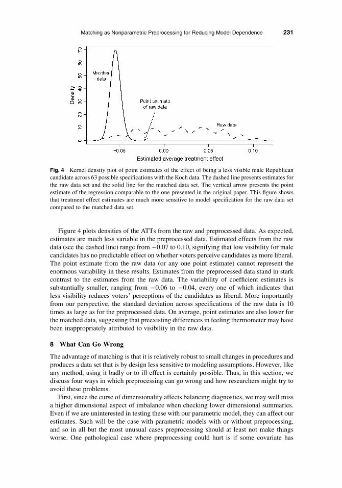
Figure 4 plots densities of the ATTs from the raw and preprocessed data. As expected,estimates are much less variable in the preprocessed data. Estimated effects from the rawdata (see the dashed line) range from �0.07 to 0.10, signifying that low visibility for malecandidates has no predictable effect on whether voters perceive candidates as more liberal.The point estimate from the raw data (or any one point estimate) cannot represent theenormous variability in these results. Estimates from the preprocessed data stand in starkcontrast to the estimates from the raw data. The variability of coefficient estimates issubstantially smaller, ranging from �0.06 to �0.04, every one of which indicates thatless visibility reduces voters’ perceptions of the candidates as liberal. More importantlyfrom our perspective, the standard deviation across specifications of the raw data is 10times as large as for the preprocessed data. On average, point estimates are also lower forthe matched data, suggesting that preexisting differences in feeling thermometer may havebeen inappropriately attributed to visibility in the raw data.

8 What Can Go Wrong

The advantage of matching is that it is relatively robust to small changes in procedures andproduces a data set that is by design less sensitive to modeling assumptions. However, likeany method, using it badly or to ill effect is certainly possible. Thus, in this section, wediscuss four ways in which preprocessing can go wrong and how researchers might try toavoid these problems.

First, since the curse of dimensionality affects balancing diagnostics, we may well missa higher dimensional aspect of imbalance when checking lower dimensional summaries.Even if we are uninterested in testing these with our parametric model, they can affect ourestimates. Such will be the case with parametric models with or without preprocessing,and so in all but the most unusual cases preprocessing should at least not make thingsworse. One pathological case where preprocessing could hurt is if some covariate has

Fig. 4 Kernel density plot of point estimates of the effect of being a less visible male Republicancandidate across 63 possible specifications with the Koch data. The dashed line presents estimates forthe raw data set and the solid line for the matched data set. The vertical arrow presents the pointestimate of the regression comparable to the one presented in the original paper. This figure showsthat treatment effect estimates are much more sensitive to model specification for the raw data setcompared to the matched data set.


a huge effect on the outcome variable and preprocessing slightly reduces balance on thisvariable but improves it for all the others. A researcher might be fooled into choosinga matching trade-off like this if he or she were not aware of the large effect of thiscovariate. Carefully evaluating what covariates are likely to have the largest effects, andusing multiple measures of balance, are essential to avoid this pitfall.

Second, as with all statistical methods, a bias-variance trade-off exists for matching.If we drop many observations during preprocessing, and balance is not substantiallyimproved, the mean squared error (or other mean-variance summary) of the estimatedcausal effect might actually increase. Users must pay close attention to this trade-offduring the process of matching, but unfortunately no precise rules exist for how to makethese choices. In particular, the methodological literature offers no formal estimates ofmean squared error and so in marginal cases it can be difficult to know whether or howmuch preprocessing will help. Of course, dropping observations does not necessarily meanthat preprocessing is worse since improving balance can also increase efficiency, and inany event including imbalanced observations requiring extrapolation in a parametric anal-ysis merely produces false precision. So although estimated standard errors may increasein some cases with preprocessing, they would likely be more accurate. Moreover, in manysituations, eliminating observations far from the rest of the data as matching does willreduce heterogeneity and thereby further reduce variance.

Third, the matching literature offers a large number of possible and seemingly ad hocprocedures. From one perspective, we might be concerned about the sensitivity of ourresults to changes in this process, just as we have been concerned with the sensitivity ofcausal effect estimates to parametric modeling assumptions. This is not normally viewedas a major issue since the right procedure is the one that maximizes balance (with n aslarge as possible), no matter how many procedures we try. By applying this criterion ina disciplined way (i.e., without consulting Y) to a large number of possible matchingprocedures, no choices are open to the analyst. Instead, researchers should merely runas many as possible and choose by maximizing balance. Unlike parametric modelingexercises, we need not choose this matching procedure or another; we merely run as manyas feasible, particularly those most likely to reduce bias and model dependence, and applythis criterion.

Finally, by dropping observations, we may wind up losing some critically importantcases or may change either the information base of our sample or, in special cases such aswhen dropping treated units, the definition of the causal effect. Examining the droppedcases provides an easy diagnostic for this problem. However, we must be alert to theproblem that if we learn that some critical units are dropped, then it may mean that noappropriate matches can be found for them. In this situation, we may be forced to concludethat the data do not contain sufficient information to answer the questions posed, no matterwhat method is chosen.

9 Concluding Remarks

Anyone using a parametric statistical technique for long enough (and it does not take verylong) will recognize the difficulty of choosing which of hundreds of possible regressions topresent in a written work. This choice is difficult, fraught with ethical and methodologicaldilemmas, and not covered in any serious way in classical statistics texts. Parametricmethods merely assume that we know the correct specification. In practice, the ‘‘correct’’specification is chosen after looking at the estimates, and so it is never clear to a readerwhether an article is a true test of a hypothesis, in the sense that the author was vulnerable


to being proved wrong, or whether the article is merely a proof of the existence of at leastone specification consistent with the author’s favored hypothesis. Researchers are oftenfrustrated with how their key causal estimates depend on specification decisions they havenot thought about and on which they have few real opinions.

We provide a way around at least part of this problem. Preprocessing raw data with thematching procedures we recommend makes familiar parametric methods a much morereliable tool of empirical analysis and, in particular, causal effect estimates become farmore insensitive to seemingly arbitrary choices in model specification. If we read an articledemonstrating that balance has been achieved for a data set, readers can worry consider-ably less that slightly different specifications than those discussed in the text will greatlyalter its empirical conclusions. Analysts using preprocessing have two chances to get theiranalyses right, in that if either the matching procedure or the subsequent parametricanalysis is specified correctly (and even if one of the two is incorrectly specified), causalestimates will still be consistent.

10 Appendix: Matching Software

A variety of excellent software is available to perform matching (Parsons 2000, 2001;Abadie et al. 2002; Becker and Ichino 2002; Bergstralh and Kosanke 2003; Leuven andSianesi 2004; Sekhon 2004; Hansen 2005). However, each program implements onlya specialized subset of available statistical procedures. Moreover, they are spread overa range of different languages and packages, which normally makes it impractical to usemore than one for any applied project. Thus, as a companion to and in the same spirit asthis paper, we have written software (called MatchIt, available at http://gking.harvard.edu/matchit) that implements the vast majority of the matching procedures suggested in thediverse scholarly literatures on this subject. Where possible, MatchIt builds on and incor-porates existing packages and, across all the specialized techniques, MatchIt offers a sin-gle, simple, and unified syntax. Adding procedures to MatchIt is also easy.

MatchIt operates with a single command that takes an existing data set and produces asoutput a single preprocessed matched data set. The preprocessed data set can then be usedby standard parametric software just as one would have used the original data set. MatchItalso works seamlessly with the general-purpose statistics program, Zelig (Imai, King, andLau 2006), so that output from MatchIt can be fed into Zelig without any extra steps.MatchIt and Zelig are freely available and run under many operating systems via the opensource and free statistical program R.

References

Abadie, Alberto, David Druckker, Jane Leber Herr, and Guido W. Imbens. 2002. Implementing matching

estimators for average treatment effects in stata. The Stata Journal 1:1–18.

Abadie, Alberto, and Guido Imbens. 2006a. Estimation of the conditional variance in paired experiments. KSG

working paper. http://ksghome.harvard.edu/;.aabadie.academic.ksg/cve.pdf (accessed September 1, 2006).

———. 2006b. Large sample properties of matching estimators for average treatment effects. Econometrica

74:235–67.

Becker, Sascha O., and Andrea Ichino. 2002. Estimation of average treatment effects based on propensity scores.

The Stata Journal 2:358–77.

Bergstralh, Erik, and Jon Kosanke. 2003. dist, gmatch, and vmatch: SAS macros. Mayo Clinic, Division of

Biostatistics. http://mayoresearch.mayo.edu/mayo/research/biostat/sasmacros.cfm (accessed September 1, 2006).

Bishop, Christopher M. 1995. Neural networks for pattern recognition. Oxford: Oxford University Press.

Black, Dan A., and Jeffrey A. Smith. 2004. How robust is the evidence on the effects of college quality?

Evidence from matching. Journal of Econometrics 121:99–124.




http://ksghome.harvard.edu/~.aabadie.academic.ksg/cve.pdf

http://mayoresearch.mayo.edu/mayo/research/biostat/sasmacros.cfm

Carpenter, Daniel P. 2002. Groups, the media, agency waiting costs, and FDA drug approval. American Journal

of Political Science 46(July):490–505.

Cochran, William G. 1968. The effectiveness of adjustment by subclassification in removing bias in observa-

tional studies. Biometrics 24:295–313.

Cochran, William G., and Donald B. Rubin. 1973. Controlling bias in observational studies: A review. Sankhya:

The Indian Journal of Statistics, Series A 35(Part 4):417–66.

Cox, David R. 1958. Planning of experiments. New York: John Wiley.

Dehejia, Rajeev H., and Sadek Wahba. 1999. Causal effects in nonexperimental studies: Re-evaluating the

evaluation of training programs. Journal of the American Statistical Association 94(December):1053–62.

Diamond, Alexis, and Jasjeet Sekhon. 2005. Genetic matching for estimating causal effects: A new method of

achieving balance in observational studies. http://sekhon.berkeley.edu/ (accessed September 1, 2006).

Fisher, Ronald A. 1935. The design of experiments. London: Oliver and Boyd.

Frolich, Markus. 2004. Finite sample properties of propensity score matching and weighting estimators. Review

of Econometrics and Statistics 86:77–90.

Glazerman, Steve, Dan M. Levy, and David Myers. 2003. Nonexperimental versus experimental estimates

of earnings impacts. The Annals of the American Academy of Political and Social Science 589(September):

63–93.

Goldberger, Arthur. 1991. A course in econometrics. Cambridge, MA: Harvard University Press.

Gu, Xing S., and Paul R. Rosenbaum. 1993. Comparison of multivariate matching methods: Structures, dis-

tances, and algorithms. Journal of Computational and Graphical Statistics 2:405–20.

Hansen, Ben B. 2004. Full matching in an observational study of coaching for the SAT. Journal of the American

Statistical Association 99:609–18.

———. 2005. Optmatch: Software for optimal matching. http://www.stat.lsa.umich.edu/;bh/optmatch.html

(accessed September 1, 2006).

Heckman, James J., Hidehiko Ichimura, Jeffrey A. Smith, and Petra E. Todd. 1998. Characterizing selection bias

using experimental data. Econometrica 66:1017–98.

Heckman, James J., Hidehiko Ichimura, and Petra E. Todd. 1997. Matching as an econometric evaluation

estimator: Evidence from evaluating a job training program. Review of Economic Studies 64:605–54.

Heckman, James J., and Richard Robb. 1985. Alternative methods for evaluating the impacts of interventions. In

Longitudinal analysis of labor market data, ed. J.Heckman andB.Singer;Cambridge:CambridgeUniversityPress.

Hirano, Keisuke, Guido W. Imbens, and Geert Ridder. 2003. Efficient estimation of average treatment effects

using the estimated propensity score. Econometrica 71(July):1161–89.

Ho, Daniel E., Kosuke Imai, Gary King, and Elizabeth A. Stuart. 2006. Replication data set for ‘matching

as nonparametric preprocessing for reducing model dependence in parametric causal inference’. http://

id.thedata.org/hdl%3A1902.1%2FYVDZEQIYDS hdl:1902.1/YVDZEQIYDS UNF:3:QV0mYCd8eVþmJg

WDnYct5g55 Murray Research Archive [distributed by DDI].

Hoeting, Jennifer A., David Madigan, Adrian E. Raftery, and Chris T. Volinsky. 1999. Bayesian model aver-

aging: A tutorial. Statistical Science 14:382–417.

Holland, PaulW. 1986. Statistics and causal inference. Journal of the American Statistical Association 81:945–60.

Iacus, Stefano, and Giuseppe Porro. 2006. Random recursive partitioning: A matching method for the estimation

of the average treatment effect. UNIMI—Research Papers in Economics, Business, and Statistics. Economics.

Working paper 9. http://services.bepress.com/unimi/economics/art9 (accessed September 1, 2006).

Imai, Kosuke, and Gary King. 2004. Did illegal overseas absentee ballots decide the 2000 U.S. presidential

election? Perspectives on Politics 2(September):537–49.

Imai, Kosuke, Gary King, and Olivia Lau. 2006. Zelig: Everyone’s statistical software. http://gking.harvard.edu/

zelig (accessed September 1, 2006).

Imai, Kosuke, Gary King, and Elizabeth A. Stuart. 2006. Misunderstandings among experimentalists and obser-

vationalists: Balance test fallacies in causal inference. http://gking.harvard.edu/files/abs/matchse-abs.shtml

(accessed September 1, 2006).

Imai, Kosuke, and David A. van Dyk. 2004. Causal inference with general treatment regimes: Generalizing the

propensity score. Journal of the American Statistical Association 99(September):854–66.

Imbens, Guido W. 2004. Nonparametric estimation of average treatment effects under exogeneity: A review.

Review of Economics and Statistics 86:4–29.

King, Gary. 1989. Unifying political methodology: The likelihood theory of statistical inference. Ann Arbor:

Michigan University Press.

King, Gary, James Honaker, Anne Joseph, and Kenneth Scheve. 2001. Analyzing incomplete political science

data: An alternative algorithm for multiple imputation. American Political Science Review 95(March):49–69.

http://gking.harvard.edu/files/abs/evil-abs.shtml (accessed September 1, 2006).


http://sekhon.berkeley.edu/

http://www.stat.lsa.umich.edu/~bh/optmatch.html

http://id.thedata.org/hdl%3A1902.1%2FYVDZEQIYDS

http://id.thedata.org/hdl%3A1902.1%2FYVDZEQIYDS

http://services.bepress.com/unimi/economics/art9

http://gking.harvard.edu/zelig

http://gking.harvard.edu/zelig

http://gking.harvard.edu/files/abs/matchse-abs.shtml

http://gking.harvard.edu/files/abs/evil-abs.shtml

bmacmillen

Sticky Note

CORRECTION: Ho Daniel E, Imai Kosuke, King Gary, Stuart Elizabeth A. "Replication data set for matching as nonparametric preprocessing for reducing model dependence in parametric causal inference". (2006) http://id.thedata.org/hdl%3A1902.1%2FYVDZEQIYDS hdl:1902.1/YVDZEQIYDS UNF:3:QV0mYCd8eV+mJgWDnYct5g== Murray Research Archive [Distributor]

King, Gary, Robert O. Keohane, and Sidney Verba. 1994. Designing social inquiry: Scientific inference in

qualitative research. Princeton, NJ: Princeton University Press.

King, Gary, and Langche Zeng. 2006. The dangers of extreme counterfactuals. Political Analysis 14:131–59.

http://gking.harvard.edu/files/abs/counterft-abs.shtml (accessed September 1, 2006).

———. 2007. When can history be our guide? The pitfalls of counterfactual inference. International Studies

Quarterly (March). http://gking.harvard.edu/files/abs/counterf-abs.shtml.

Koch, Jeffrey M. 2002. Gender stereotypes and citizens’ impressions of house candidates’ ideological orienta-

tion. American Journal of Political Science 46:453–62.

Lechner, Michael. 2000. A note on the common support problem in applied evaluation studies. University of

St. Galen. http://www.siaw.unisg.ch/lechner (accessed September 1, 2006).

Leuven, Edwin, and Barbara Sianesi. 2004. PSMATCH2: Stata module to perform full Mahalanobis and pro-

pensity score matching, common support graphing, and covariate imbalance testing. EconPapers. http://

econpapers.repec.org/software/bocbocode/S432001.htm (accessed September 1, 2006).

Lewis, David K. 1973. Counterfactuals. Cambridge, MA: Harvard University Press.

McCullagh, Peter, and James A. Nelder. 1989. Generalized linear models. 2nd ed. Monograph on statistics and

applied probability 37. New York (NY): Chapman & Hall/CRC.

Meng, Xiao-Li, and Martin Romero. 2003. Discussion: Efficiency and self-efficiency with multiple imputation

inference. International Statistical Review 71:607–18.

Neyman, Jerzy. 1935. Statistical problems in agricultural experiments. Supplement to the Journal of the Royal

Statistical Society 2:107–80.

Parsons, Lori S. 2000. Using SAS software to perform a case-control match on propensity score in an obser-

vational study. http://www2.sas.com/proceedings/sugi25/25/po/25p225.pdf (accessed September 1, 2006).

———. 2001. Reducing bias in a propensity score matched-pair sample using greedy matching techniques.

http://www2.sas.com/proceedings/sugi26/p214-26.pdf (accessed September 1, 2006).

Quandt, Richard. 1972. Methods of estimating switching regressions. Journal of the American Statistical

Association 67:306–10.

Robins, James M., and Andrea Rotnitzky. 2001. Comment on the Peter J. Bickel and Jaimyoung Kwon,

‘Inference for semiparametric models: Some questions and an answer’. Statistica Sinica 11:920–36.

———. Forthcoming. Inverse probability weighting estimation in survival analysis. Encyclopedia of

Biostatistics.

Rosenbaum, Paul R. 1984. The consequences of adjusting for a concomitant variable that has been affected by

the treatment. Journal of the Royal Statistical Society, Series A 147:656–66.

———. 1986. Dropping out of high school in the United States: An observational study. Journal of Educational

Statistics 11:207–24.

———. 1989. Optimal matching for observational studies. Journal of the American Statistical Association

84:1024–32.

———. 2002. Observational studies. 2nd ed. New York: Springer.

Rosenbaum, Paul R., and Donald B. Rubin. 1983. The central role of the propensity score in observational

studies for causal effects. Biometrika 70:41–55.

———. 1984. Reducing bias in observational studies using subclassification on the propensity score. Journal of

the American Statistical Association 79:516–24.

———. 1985. The bias due to incomplete matching. Biometrics 41:103–16.

Rosenbaum, Paul R., and Jeffrey H. Silber. 2001. Matching and thick description in an observational study of

mortality after surgery. Biostatistics 2:217–32.

Roy, A. D. 1951. Some thoughts on the distribution of earnings. Oxford Economic Papers 3:135–46.

Rubin, Donald B. 1973. The use of matched sampling and regression adjustment to remove bias in observational

studies. Biometrics 29:185–203.

———. 1974. Estimating causal effects of treatments in randomized and nonrandomized studies. Journal of

Educational Psychology 6:688–701.

———. 1978. Bayesian inference for causal effects: The role of randomization. The Annals of Statistics 6:

34–58.

———. 1979. Using multivariate matched sampling and regression adjustment to control bias in observational

studies. Journal of the American Statistical Association 74:318–28.

———. 1987. Multiple imputation for nonresponse in surveys. New York: John Wiley.

———. 2001. Using propensity scores to help design observational studies: Application to the tobacco litiga-

tion. Health Services & Outcomes Research Methodology 2(December):169–88.

Rubin, Donald B., and Elizabeth A. Stuart. 2006. Affinely invariant matching methods with discriminant

mixtures of proportional ellipsoidally symmetric distributions. Annals of Statistics 34:1814–1826.


http://gking.harvard.edu/files/abs/counterft-abs.shtml

http://gking.harvard.edu/files/abs/counterf-abs.shtml

http://www.siaw.unisg.ch/lechner

http://econpapers.repec.org/software/bocbocode/S432001.htm

http://econpapers.repec.org/software/bocbocode/S432001.htm

http://www2.sas.com/proceedings/sugi25/25/po/25p225.pdf

http://www2.sas.com/proceedings/sugi26/p214-26.pdf

Rubin, Donald B., and Neal Thomas. 1992. Characterizing the effect of matching using linear propensity score

methods with normal distributions. Biometrika 79:797–809.

———. 1996. Matching using estimated propensity scores, relating theory to practice. Biometrics 52:249–64.

———. 2000. Combining propensity score matching with additional adjustments for prognostic covariates.

Journal of the American Statistical Association 95:573–85.

Sekhon, Jasjeet S. 2004. Multivariate and propensity score matching software. http://jsekhon.fas.harvard.edu/

matching/ (accessed September 1, 2006).

Smith, Herbert L. 1997. Matching with multiple controls to estimate treatment effects in observational studies.

Sociological Methodology 27:325–53.

Smith, Jeffrey A., and Petra E. Todd. 2005. Does matching overcome LaLonde’s critique of nonexperimental

estimators? Journal of Econometrics 125(March–April):305–53.

Stuart, Elizabeth A. 2004. Matching methods for estimating causal effects using multiple control groups. Ph.D.

thesis, Department of Statistics, Harvard University.


http://jsekhon.fas.harvard.edu/matching/

http://jsekhon.fas.harvard.edu/matching/

Matching as Nonparametric Preprocessing for Reducing - Gary King

Documents

Transcript of Matching as Nonparametric Preprocessing for Reducing - Gary King