Score matching and nonparametric estimators of drift...
54
Score matching and nonparametric estimators of drift functions for stochastic differential equations Manfred Opper joint work with Philip Batz, Andreas Ruttor, April 13, 2016 Manfred Opper joint work with Philip Batz, Andreas Ruttor, Nonparametric estimation of drift April 13, 2016 1 / 29
Transcript of Score matching and nonparametric estimators of drift...

Score matching and nonparametric estimators of driftfunctions for stochastic differential equations
Manfred Opper
joint work with Philip Batz, Andreas Ruttor,
April 13, 2016
Manfred Opper joint work with Philip Batz, Andreas Ruttor, (AI group, TU Berlin)Nonparametric estimation of drift April 13, 2016 1 / 29

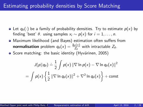
Estimating probability densities by Score Matching
Let qθ(·) be a family of probability densities. Try to estimate p(x) byfinding ’best’ θ. using samples xi ∼ p(x) for i = 1, . . . , n.
Maximum likelihood (and Bayes) estimation often suffers from
normalisation problem qθ(x) = qθ(x)Zθ
with intractable Zθ.
Score matching: the basic identity (Hyvarinen, 2005)
J(p‖qθ).
=1
2
∫p(x) ‖∇ ln p(x)−∇ ln qθ(x)‖2
=
∫p(x)
{1
2‖∇ ln qθ(x)‖2 +∇2 ln qθ(x)
}+ const
Manfred Opper joint work with Philip Batz, Andreas Ruttor, (AI group, TU Berlin)Nonparametric estimation of drift April 13, 2016 2 / 29

Use minimisation of empirical loss
n∑i=1
{1
2‖∇ ln qθ(xi )‖2 +∇2 ln qθ(xi )
}independent of Zθ !
Nonparametric extension (Sriperumbudur, Fukumizu, Kumar, Grettonand Hyvarinen, 2014). Set ψ(x)
.= ln q(x)
n∑i=1
{1
2‖∇ψ(xi )‖2 +∇2ψ(xi )
}+
1
2‖ψ(·)‖2
RKHS
yields estimate of ∇ ln p(x) !
Manfred Opper joint work with Philip Batz, Andreas Ruttor, (AI group, TU Berlin)Nonparametric estimation of drift April 13, 2016 3 / 29

Some applications of score matching
Learning structure of graphical models
Finding modes of probability densities
Gradient free Hamiltonian Monte Carlo
Sequential importance sampling
...
Manfred Opper joint work with Philip Batz, Andreas Ruttor, (AI group, TU Berlin)Nonparametric estimation of drift April 13, 2016 4 / 29

Outline
Problem of learning drift functions for stochastic differential equations
Nonparametric estimates using a generalisation of score matching
Applications to Langevin models
Relation to Maximum likelihood and Bayes
Kullback–Leibler divergence, control and a normalizer
Future work and open problems
Manfred Opper joint work with Philip Batz, Andreas Ruttor, (AI group, TU Berlin)Nonparametric estimation of drift April 13, 2016 5 / 29

Stochastic differential equations
Dynamics defined by SDEs for Z ∈ Rd .
dZt = g(Zt)︸ ︷︷ ︸Drift
dt + σ(Zt)︸ ︷︷ ︸Diffusion
× dWt︸︷︷︸Wiener process
Limit of discrete time process
Zt+∆ − Zt = g(Zt)∆ + σ(Zt)√
∆ εt .
with εt i.i.d. Gaussian for ∆→ 0.
Learn the function g(·) from a set of (noise free) observationsz(t1), z(t2), . . . , z(tn).
Manfred Opper joint work with Philip Batz, Andreas Ruttor, (AI group, TU Berlin)Nonparametric estimation of drift April 13, 2016 6 / 29

Nonparametric (Gaussian process) approach
Use a Gaussian Process prior g(·) ∼ GP(0,K (z , z ′)) over drift functions.(Papaspilioupoulis, Pokern, Roberts and Stuart 2012).
0 10 20 30 40 50 60 70 80 90 100!2
!1.5
!1
!0.5
0
0.5
1
1.5
2
2.5
Manfred Opper joint work with Philip Batz, Andreas Ruttor, (AI group, TU Berlin)Nonparametric estimation of drift April 13, 2016 7 / 29

Likelihood for densely observed path
In Euler discretization the SDE looks likeZt+∆t − Zt = g(Zt)∆ +
√∆ εt , for ∆→ 0.
Hence the likelihood for the drift is
p(Z0:T |g) ∝ exp
[− 1
2∆
∑t
||Zt+∆ − Zt ||2]×
exp
[−1
2
∑t
||g(Zt)||2 ∆ +∑
t
g(Zt) · (Zt+∆ − Zt)
].
allows for simple GP based estimation of the function g(·).
This essentially leads to the estimate
g(z) ≈ E[
Zt+∆−Zt
∆ |Zt = z]. Works well for ∆→ 0.
Manfred Opper joint work with Philip Batz, Andreas Ruttor, (AI group, TU Berlin)Nonparametric estimation of drift April 13, 2016 8 / 29

For not so small ∆ it does not work well ! Data fromdz = (z − z3)dt + dW .
199.5 200.0 200.5 201.0 201.5
−1.
4−
1.2
−1.
0−
0.8
t
X(t
)
●
●
●
●
●
−2 −1 0 1 2
−6
−4
−2
02
46
xf(
x)
Estimation from sparse observations in time not trivial ! Approximationusing imputation of hidden process possible (Ruttor, Batz and Opper,2013).
Manfred Opper joint work with Philip Batz, Andreas Ruttor, (AI group, TU Berlin)Nonparametric estimation of drift April 13, 2016 9 / 29

Drift estimation from empirical density only
Given stationary density p(z) of the process. Determine the drift g ?Assume that σ(·) is known and g(z) = r(z) + f (z), with r(z) known.
Partial answer:’minimal’ solution minimising a quadratic functional
1
2
∫p(z) f (z) · A−1(z)f (z) dz
Lagrange–functional
1
2
∫f (z) · A−1(z)f (z) dz −
∫ψ(z) {Lp(z)−∇ · (f (z)p(z))} dz
with Fokker–Planck operator corresponding to r(z)
Lp(z) = −∇ · (r(z)p(z)) +1
2tr[∇∇>(D(z)p(z))
]with D(z)
.= σ(z)σ(z)>.
Manfred Opper joint work with Philip Batz, Andreas Ruttor, (AI group, TU Berlin)Nonparametric estimation of drift April 13, 2016 10 / 29

Variation yields f (z) = A(z)∇ψ(z). Inserting back into Lagrangean yieldsdual functional
ε[ψ] =
∫ {1
2∇ψ(z) · A(z) ∇ψ(z) + L∗ψ(z)
}p(z)dz
with L∗ adjoint operator which fulfils∫ψ(z)Lp(z)dz =
∫p(z)L∗ψ(z)dz
and is given by
L∗ψ(z) = r(z) · ∇ψ(z) +1
2tr[D(z)∇∇>ψ(z)
]For ’thermal equilibrium’ A = I and D = 2I and r = 0 this corresponds toscore matching ! Stationary density p(z) ∝ e2ψ(z) and f (z) = ∇ψ(x)
Manfred Opper joint work with Philip Batz, Andreas Ruttor, (AI group, TU Berlin)Nonparametric estimation of drift April 13, 2016 11 / 29
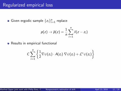
Regularized empirical loss
Given ergodic sample {zi}ni=1 replace
p(z)→ p(z) =1
n
n∑i=1
δ(z − zi )
Results in empirical functional
Cn∑
i=1
{1
2∇ψ(zi ) · A(zi ) ∇ψ(zi ) + L∗ψ(zi )
}
+1
2
∫ ∫ψ(z)K−1(z , z ′)ψ(z ′) dzdz ′
regularised by kernel K .
Manfred Opper joint work with Philip Batz, Andreas Ruttor, (AI group, TU Berlin)Nonparametric estimation of drift April 13, 2016 12 / 29

Regularized empirical loss
Given ergodic sample {zi}ni=1 replace
p(z)→ p(z) =1
n
n∑i=1
δ(z − zi )
Results in empirical functional
Cn∑
i=1
{1
2∇ψ(zi ) · A(zi ) ∇ψ(zi ) + L∗ψ(zi )
}+
1
2
∫ ∫ψ(z)K−1(z , z ′)ψ(z ′) dzdz ′
regularised by kernel K .
Manfred Opper joint work with Philip Batz, Andreas Ruttor, (AI group, TU Berlin)Nonparametric estimation of drift April 13, 2016 12 / 29

Variation wrt ψ yields
ψ(z) + Cn∑
j=1
L∗z ′ [ψ] K (z , z ′)z ′=zj= 0
regularised version of equation (valid for any function h(·))∫p(z ′)L∗z ′ [ψ]h(z ′)dz ′ =
∫h(z ′)Lz ′ [ψ]p(z ′)dz ′ = 0
applied to p → p and hz (z ′) = K (z , z ′).
If ∇ψ(z) known at all sample points z = zi , get ψ(z) for all z .
Take gradient
∇ψ(zi ) + Cn∑
j=1
L∗z ′ [ψ]∇zK (z , z ′)z=zi ,z ′=zj= 0
Manfred Opper joint work with Philip Batz, Andreas Ruttor, (AI group, TU Berlin)Nonparametric estimation of drift April 13, 2016 13 / 29

Langevin dynamics
Classical mechanics in terms of (generalized) coordinates andvelocities X ,V ∈ Rd
dXt = Vtdt, dVt = gv (Xt ,Vt)dt + σv (Xt ,Vt)dWt .
If drift is of the form gv (x , v) = rv (x , y) +∇vψ(x , v) use functionalfor estimation
ε[ψ] =
∫p(x , v)
{L∗ψ(x , v) +
1
2(∇vψ(x , v))2
}dx dv
where
L∗ψ(x , v) =
(v · ∇x + rv (x , v) · ∇v +
1
2tr(Dv (x , v)∇>v ∇v )
)ψ(x , v) .
Manfred Opper joint work with Philip Batz, Andreas Ruttor, (AI group, TU Berlin)Nonparametric estimation of drift April 13, 2016 14 / 29

Condition fv (x , v) = ∇vφ(x , v) restricts the velocity dependency!
Possible choice
fv (x , v) = f (x)− Λv = ∇v
{v · f (x)− 1
2v · Λv
},
Note: If rv = −Λv then L∗ψ(x , v) = L∗(v · f (x)) is independent ofthe diffusion term Dv (x , v):→ Estimate f (x) without knowing the diffusion.
Manfred Opper joint work with Philip Batz, Andreas Ruttor, (AI group, TU Berlin)Nonparametric estimation of drift April 13, 2016 15 / 29

Example: Double well
f (x , v) = 4(x − x3)− λv
−1.5 −0.5 0.5 1.0 1.5
−6
−2
24
6
x
f(x,
v)
v = −1v = 0v = 1
●
● ●
● ● ●● ● ●
●●●
●●
●●●●
●●●●●●●●●●●●●
500 1000 2000 50000.
10.
20.
51.
02.
0
Obs No.
MS
E
Manfred Opper joint work with Philip Batz, Andreas Ruttor, (AI group, TU Berlin)Nonparametric estimation of drift April 13, 2016 16 / 29

Example: Nonconservative force
f (1)(x) = x (1)(1− (x (1))2 − (x (2))2)− x (2)
f (2)(x) = x (2)(1− (x (1))2 − (x (2))2)− x (1)
Polynomial kernel with p = 4 and n = 2000
−3 −2 −1 0 1 2 3
−3
−1
01
23
Manfred Opper joint work with Philip Batz, Andreas Ruttor, (AI group, TU Berlin)Nonparametric estimation of drift April 13, 2016 17 / 29

Cart and Pole model
q
f (x) = a sin x and r(v) = −λv and diffusion Dv = (σ cos(x))2.
0 2 4 6 8 10
−4
04
t
X(t
)
●
●
●●●●●●●
●●●●
●
●●●
●
●●
●
●●●
●●●●●
●●●●
●
●●
●
●
●●
●
●
●
●●
●
●
●●
●
●
●●
●
●
●●
●
●
●●●
●
●●●●●
●●●
●
●●●
●
●●●
●
●●●
●
●
●●
●
●
●●
●
●
●●
●
●
●●●
●●●●●
●●●
●
●
●●
●
●
●●
●
●
●●
●
●
●●
●
●
●●
●
●
●●●
●
●
●●
●
●
●●●
●
●
●●
●
●
●●
●
●
●
●●
●
●
●●
●
●
●
●
●
●
●
●●
●
●●●
●
●●●●
●
●
●●
●
●
●●
●
●
●●●
●
●●●
●
●
●●
●
●
●●
●
●
●
●
●
●
●
●●
●
●
●
●
●
●
●
●●
●
●
●
●●
●
●
●●
●
●
●
●●
●
●
●
●●
●
●
●
●
●
●
●
●●
●
●
●
●
●
●
●
●●
●
●
●
●●
●
●
●●
●
●
●
●●
●
●
●
●
●
●
●
●●
●
●
●
●
●
●
●
●●
●
●
●
●●
●
●
●
●●
●
●
●●
●
●
●
●●
●
●
●
●
●
●
●
●●
●
●
●
●●
●
●
●●
●
●
●
●
●
●
●
●●
●
●
●●
●
●
●●
●
●●●
●●●
●
●
●●
●
●
●●●
●
●●
●
●
●●
●
●●●
●
●●
●
●
●
●
●
●●●
●
●
●●
●
●
●●
●
●●●
●●●
●
●●●
●
●●●●
●
●
●●
●
●
●●
●
●
●●●
●
●●
●
●
●●
●
●
●●
●
●
●●
●
●
●●
●
●
●●
●
●
●
●
●
●
●
●●
●
●
●
●●
●
●
●
●
●
●
●
●
●
●●
●
●
●
●●
●
●
●
●
●●
●
●
●
●
●●
●
●
●
●●
●
●
●
●
●
●
●
●
●
●●
●
●
●
●
●
●
●
●
●
●
●
●●
●
●
●
●
●
●●
●
●
●
●
●
●
●
●
●
●
●
●
●
●
●
●●
●
●
●
●●
●
●
●
●●
●
●
●
●
●
●
●
●●
●
●
●
●●
●
●
●
●
●
●
●
●●
●
●
●●
●
●
●●●
●
●
●●
●
●
●●
●
●
●●
●
●
●●
●
●
●●
●
●
●●
●
●
●●
●
●
●●
●
●
●●
●
●
●
●●
●
●
●
●
●
●
●
●●
●
●
●
●●
●
●
●
●●
●
●
●
●●
●
●
●
●
●
●
●
●●
●
●
●●
●
●
●●
●
●
●●
●
●
●
●●
●
●
●●
●
●
●●●
●
●●
●
●
●●
●
●
●
●●
●
●
●●
●
●
●●
●
●
●
●
●
●
●
●●
●
●
●
●●
●
●
●
●●
●
●
●
●
●
●
●
●
●
●
●
●
●●
●
●
●
●●
●
●
●
●●
●
●
●
●
●●●
●
●
●
●
●
●
●
●
●
●
●
●
●
●
●
●
●
●●●
●
●
●
●
●
●●
●
●
●
●
●●
●
●
●
●
●●
●
●
●
●●
●
●
●
●
●
●
●
●
●
●●
●
●
●
●
●
●
●
●
●
●●
●
●
●
●●
●
●
●
●●
●
●
●
●●
●
●
●
●●
●
●
●
●●
●
●
●
●●
●
●
●
●
●
●
●
●●
●
●
●
●●
●
●
●
●
●
●
●
●
●●
●
●
●
●
●
●
●
●
●●
●
●
●
●●
●
●
●
●●
●
●
●●
●
●
●
●●
●
●
●
●●
●
●
●
●
●●
●
●
●
●
●
●
●
●
●
●●
●
●
●
●
●●
●
●
●
●
●
●●●●
●
●
●
●
●●
●
●
●
●
●
●
●
●
●
●●
●
●
●
●
●
●●●●●
●
●
●
●
●
●●
●
●
●
●
●
●●
●
●
●
●
●
●●
●
●
●
●
●
●
●
●
●
●
●
●●●●
●
●
●
●
●
●
●●
●
●
●
●
●
●●
●
●
●
●
●
●
●
●
●
●
●
●
●●
●
●
●
●
●●
●
●
●
●●
●
●
●
●●
●
●
●
●●
●
●
●
●●
●
●
●
●
●
●
●
●
●
●
●
●●
●
●
●
●
●●
●
●
●
●
●●
●
●
●
●
●
●●
●
●
●
●
●
●●●●
●
●
●
●
●
●●
●
●
●
●
●●
●
●
●
●
●●
●
●
●
●
●
●
●
●
●
●
●
●
●
●
●
●
●
●
●●●
●
●
●
●
●
●●●
●
●
●
●
●
●
●
●
●
●
●
●
●●
●
●
●
●
●
●
●
●●
●
●
●
●
●
●
●
●
●
●
●
●
●
●●●●●●
●
●
●
●
●
●●
●
●
●
●
●●
●
●
●
●
●
●
●
●
●
●●
●
●
●●
●
●
●
●
●
●
●
●●
●
●
●●
●
●
●
●●
●
●
●
●●
●
●
●
●●
●
●
●
●
●
●
●
●
●●
●
●
●
●
●
●
●
●
●
●●
●
●
●
●●
●
●
●
●●
●
●
●
●●
●
●
●
●●
●
●
●
●●
●
●
●
●
●
●
●
●
●
●
●
●
●
●
●
●
●
●
●●
●
●
●
●●
●
●
●
●●
●
●
●
●●
●
●
●
●
●
●
●
●
●
●●
●
●
●
●
●●
●
●
●
●
●
●
●
●
●●
●
●
●
●
●
●
●
●
●
●
●
●●
●
●
●
●
●
●●
●
●
●
●
●
●
●
●
●
●
●
●
●
●
●
●
●
●
●
●
●
●
●
●
●
●
●
●
●
●
●
●
●
●
●
●
●
●
●
●
●
●
●●●
●
●
●
●
●●
●
●
●
●
●●
●
●
●
●
●
●
●
●
●
●
●
●
●
●
●●●
●
●
●
●
●
●
●
●
●
●
●●
●
●
●
●
●●
●
●
●
●●
●
●
●
●
●●
●
●
●
●●
●
●
●
●
●●
●
●
●
●●
●
●
●
●
●
●
●
●
●
●●
●
●
●
●●
●
●
●
●●
●
●
●
●
●●
●
●
●
●
●
●
●
●●
●
●
●●
●
●
●●
●
●
●
●●
●
●
●
●
●
●
●
●●
●
●
●
●
●
●
●
●
●
●
●
●
●
●
●
●
●
●
●
●
●●
●
●
●●●●●●●
●
●●●●
●●●
●●●
●●●
●
●●
●
●
●●
●
●
●●
●
●
●
●●
●
●
●
●●
●
●
●
●
●
●
●
●
●
●
●
●
●
●
●
●
●
●●
●
●
●
●●
●
●
●
●
●
●
●
●●
●
●
●
●●
●
●
●
●
●
●
●
●
●●
●
●
●
●
●
●
●
●
●
●
●
●●●
●
●
●
●
●
●●●
●
●
●
●
●
●●
●
●
●
●●
●
●
●
●●
●
●
●
●●
●
●
●●
●
●
●
●●
●
●
●●
●
●
●
●
●
●
●
●
●
●●
●
●
●
●
●●●
●
●
●
●
●●
●
●
●
●
●
●
●
●
●●
●
●
●
●●
●
●
●
●
●
●
●
●●
●
●
●
●●
●
●
●
●
●
●
●
●●
●
●
●●
●
●
●
●●
●
●
●●
●
●
●
●●
●
●
●
●●
●
●
●●
●
●
●
●●
●
●
●●
●
●
●
●●
●
●
●
●
●
●
●
●●
●
●
●●
●
●
●●●
●
●●●●●
●●●●●
●
●
●●
●
●
●●
●
●
●●
●
●
●●
●
●
●
●●
●
●
●●●
●
●●
●
●●●●●●
●
●●●●
●
●●
●
●●●
●
●
●
●
●
●
●
●
●
●
●●
●
●
●
●
●
●
●
●
●●
●
●
●
●●
●
●
●
●●
●
●
●
●
●
●
●
●●
●
●
●
●●
●
●
●
●●
●
●
●
●
●
●
●
●●
●
●
●
●
●●
●
●
●
●●
●
●
●
●●
●
●
●
●
●●
●
●
●
●
●●
●
●
●
●
●●
●
●
●
●●
●
●
●
●●
●
●
0 2 4 6 8 10
−5
5
t
V(t
)
●●
●●●●●
●●●
●●
●
●
●
●●
●
●
●●●
●
●
●
●
●●
●●●
●
●
●
●
●
●●
●
●
●●
●
●
●●
●
●
●●
●
●
●
●●
●
●●●
●
●
●●●
●
●●●●
●
●
●
●
●
●
●
●
●
●●
●
●
●
●●
●
●
●●
●
●
●●●
●
●●●
●
●●
●●●
●●
●
●
●●
●
●
●●
●
●
●
●
●
●
●
●
●
●●●
●
●
●●
●
●
●
●●
●
●
●●
●
●
●
●
●
●
●
●
●
●
●
●●●
●
●
●●
●
●
●
●
●
●
●
●
●
●
●
●
●
●
●
●
●●
●
●●●●
●
●●
●
●
●
●
●
●
●
●●
●
●
●●
●
●
●●
●
●
●●
●
●
●
●●
●
●
●●
●
●
●
●
●
●
●
●
●
●
●
●
●●
●
●
●
●
●
●
●
●
●
●
●
●
●●
●
●
●
●
●
●
●
●●
●
●
●
●●
●
●
●
●
●
●
●
●●
●
●
●
●
●
●
●
●
●
●
●
●
●●
●
●
●
●
●
●
●
●●
●
●
●
●
●
●
●
●●●
●
●
●●
●
●
●
●
●
●
●
●●
●
●
●
●
●
●
●
●
●
●
●
●
●●
●
●
●●
●
●
●
●
●
●
●
●●
●
●
●●
●
●
●
●
●
●
●
●
●
●●●
●
●
●
●
●
●
●
●
●
●
●
●
●●
●
●
●
●
●
●
●●
●
●●
●
●
●
●●
●
●
●●
●
●
●
●
●●●
●
●●●
●
●
●●●●
●
●●
●
●
●
●
●
●●●
●
●
●
●
●
●
●
●●
●
●●
●
●
●●
●
●
●
●
●
●
●●
●
●
●
●
●
●
●
●
●
●
●
●
●●
●
●
●
●●
●
●
●
●●
●
●
●
●
●
●
●
●
●
●
●
●
●
●
●
●
●
●
●
●
●
●
●
●
●
●
●●
●
●
●
●
●
●
●
●
●
●
●
●
●
●
●
●
●
●
●
●
●
●
●
●
●
●
●
●
●
●
●
●
●
●
●
●
●
●
●
●
●
●
●
●
●
●
●
●
●
●
●
●
●
●
●
●●
●
●
●
●
●
●
●
●
●
●
●
●
●
●
●
●
●
●
●
●
●
●●
●
●
●●●
●●
●●
●
●
●●
●
●
●
●
●
●
●●
●
●
●●
●
●
●●
●
●
●
●
●
●
●
●
●
●
●●
●
●
●
●
●
●
●
●●
●
●
●
●●
●
●
●
●
●
●
●
●
●
●
●
●
●
●
●
●
●
●●
●
●
●
●●
●
●
●●
●
●
●●
●
●
●●
●
●
●●
●
●
●
●●●
●
●●
●
●
●●●
●
●●
●
●
●
●●
●
●
●●
●
●
●
●
●
●
●
●
●
●
●
●●
●
●
●
●
●
●
●
●
●
●
●
●
●
●
●
●
●
●●
●
●
●
●
●
●
●
●
●
●
●
●
●
●
●
●
●
●
●●
●
●
●
●
●
●
●
●
●
●
●
●●
●
●●
●
●
●
●
●
●
●
●
●
●
●
●
●
●
●
●
●●
●
●
●
●
●●
●
●
●
●
●
●
●
●
●
●●
●
●
●
●
●
●
●
●
●
●●
●
●
●
●
●
●
●
●
●
●
●
●
●
●
●
●
●
●
●
●
●
●
●
●
●
●
●
●
●
●
●
●
●
●
●
●
●
●
●●
●
●
●
●
●
●
●
●
●
●
●
●
●
●
●
●
●
●●
●
●
●
●●
●
●
●
●
●
●
●
●
●
●
●
●
●
●
●
●
●
●
●●
●
●
●
●
●
●
●
●
●
●
●
●
●
●●
●
●
●
●
●
●
●
●
●
●
●
●
●
●
●
●
●
●
●
●
●
●
●
●
●
●
●
●●
●
●
●
●
●
●
●
●●
●
●
●
●●
●
●
●
●
●
●
●
●●●●●
●
●
●
●●
●
●
●
●
●
●
●
●
●
●
●
●
●
●
●
●
●
●
●
●
●
●
●
●
●
●
●
●
●
●
●
●
●
●
●●
●
●
●
●
●
●
●
●
●
●
●
●
●
●
●
●
●●●
●
●
●
●
●
●
●
●●
●
●
●
●
●
●
●
●
●
●
●
●
●
●
●
●
●
●
●
●
●
●
●
●
●●
●
●●
●
●
●●
●
●
●
●
●●
●
●
●
●
●
●
●
●
●
●
●
●
●
●
●
●
●
●●
●
●●
●
●●
●
●
●
●
●
●
●
●
●●
●
●
●
●
●●
●
●
●
●
●
●
●
●●
●
●
●●
●
●●
●
●
●
●
●
●
●
●
●
●
●
●
●
●
●●
●
●
●
●
●
●
●
●
●
●
●
●
●
●
●
●
●
●
●
●
●●●
●
●
●
●
●
●●●
●
●●
●
●
●
●
●●●
●
●
●
●
●
●
●
●
●
●●
●
●
●
●
●●
●
●
●
●
●
●
●
●
●●
●
●
●
●
●
●
●
●
●
●
●
●●
●
●
●
●●
●
●
●
●
●
●
●
●
●
●
●
●
●●
●
●
●
●●
●
●
●
●
●
●
●
●
●
●
●
●
●
●
●
●
●
●
●
●
●
●
●
●
●
●
●
●
●
●
●●
●
●
●
●
●
●
●
●
●
●
●
●
●●
●
●
●
●●
●
●
●
●●
●
●
●
●
●
●
●
●
●
●
●
●
●
●
●
●
●
●
●
●
●
●
●
●
●●
●
●
●
●
●●
●
●
●
●
●
●
●
●
●
●
●
●
●
●
●
●
●
●
●
●
●
●
●
●
●
●
●
●●
●
●
●
●
●
●
●●
●
●
●●
●
●●
●●
●
●
●
●●
●
●
●
●
●
●
●
●
●
●
●
●
●
●●
●●
●
●
●
●●
●
●
●
●
●
●
●
●
●
●
●
●
●
●
●
●
●
●
●
●
●
●
●●
●
●
●
●
●
●
●
●●
●
●
●
●
●
●
●
●
●
●
●
●
●
●
●
●
●
●
●
●
●
●
●
●
●
●
●
●
●
●
●
●
●
●
●
●
●●
●
●
●
●
●
●
●
●
●
●
●
●
●
●
●
●
●
●
●
●
●
●
●
●
●
●
●
●
●
●
●●
●
●
●
●●
●
●
●
●
●
●
●
●●
●
●
●●
●
●●●●
●
●
●
●●
●
●
●●
●
●
●
●
●
●
●
●●
●
●
●
●
●
●
●
●
●
●
●
●
●
●
●
●●
●
●●
●
●●
●
●
●●●
●●
●●●
●
●●
●
●
●
●
●
●●
●
●
●●
●
●
●
●
●
●
●
●
●
●
●
●
●
●
●
●
●
●●
●
●
●
●●
●
●
●
●●
●
●
●
●
●
●
●
●●
●
●
●
●
●
●
●
●
●
●
●
●
●
●
●
●
●
●
●
●
●
●
●
●
●
●
●●
●
●
●
●
●
●
●
●
●
●●
●
●
●●●
●
●
●
●
●
●
●
●
●
●
●
●
●
●
●
●
●
●●
●
●
●
●
●
●
●
●
●
●
●
●
●
●
●
●
●
●
●
●
●
●
●
●
●
●
●
●
●
●
●
●
●
●
●
●●
●
●
●
●
●●
●
●
●
●
●
●
●
●
●
●
●
●
●●
●
●
●
●
●
●
●
●
●
●
●
●
●
●
●
●
●
●●
●
●
●●
●
●
●
●
●
●
●
●●
●
●
●
●●
●
●
●
●
●
●
●
●●
●
●
●
●
●
●
●
●●
●
●
●●
●
●
●
●●
●
●
●
●●
●
●
●●
●
●
●
●
●
●
●
●
●
●●
●●●●●
●
●
●
●
●
●
●
●
●
●
●
●
●
●●●
●
●
●●●
●
●
●●
●
●
●●
●
●●●●●
●
●
●
●●●●
●
●
●
●
●
●
●
●
●●
●
●
●
●
●
●
●
●
●
●
●
●
●
●
●
●●
●
●
●
●
●●
●
●
●
●●
●
●
●
●
●
●
●
●●
●
●
●
●
●
●
●
●
●
●
●
●
●●
●
●
●
●●
●
●
●
●●
●
●
●
●
●
●
●
●
●
●
●
●
●
●
●●
●
●
●
●
●
●
●
●
●
●
●●
●
●
●
●
●
●
●
●
●
●
●
●
●
●●
−6 −4 −2 0 2 4 6
−10
−5
05
10
x
f(x)
Manfred Opper joint work with Philip Batz, Andreas Ruttor, (AI group, TU Berlin)Nonparametric estimation of drift April 13, 2016 18 / 29

Kernel density estimators as alternative ?
Explicit solutions to drift for Langevin models
f (i)(x) =d∑
j=1
∂E [v (i)v (j)|x ]
∂x (j)+
d∑j=1
E [v (i)v (j)|x ]∂ ln p(x)
∂x (j)− E [r (i)|x ] ,
Simplifies only for ’thermal equilibrium’ f (x) = ∇φ and Dv ∝ Σ, r = −Λvwhere Λ and Σ are diagonal with 2λi
σ2i
= β. One has then
E [v (i)v (j)|x ] = 12β δij and E [r (i)|x ] = 0.
Manfred Opper joint work with Philip Batz, Andreas Ruttor, (AI group, TU Berlin)Nonparametric estimation of drift April 13, 2016 19 / 29

Extension: Other evolution equations
Replace white noise σv (X ,V )dW → U(t)dt where U(t) Markovian.
Include noise in state variable Z = (X ,V ,U)
Example: U(t) = ±1 random telegraph process and x , v , u ∈ R withdrift gv (x , v) = −λv + f (x)
Fokker Planck → Master equation
0 = −∂x (vp(x , v , u)− ∂v [(f (x)− λv + u)p(x , v , u)]
+γ (p(x , v ,−u)− p(x , v , u))
Adjoint operator
L∗ψ = {v∂x + (u − λv)∂v}ψ + γ (ψ(x , v ,−1)− ψ(x , v , 1))
Parametrisation ψ(x , v) = vf (x) leads to functional
ε[f ] =1
2
∑u=±1
∫p(x , v , u)
{f 2(x) + 2f ′(x)v2 + 2f (x)(u − λv)
}dxdv
Manfred Opper joint work with Philip Batz, Andreas Ruttor, (AI group, TU Berlin)Nonparametric estimation of drift April 13, 2016 20 / 29

The case A = D: Likelihood for densely observed path
− ln p(Z0:T |g) =1
2
∑t
{||g(Zt)||2∆t − 2〈g(Zt), (Zt+∆t − Zt)〉
}+ const
with 〈u, v〉 .= u>D−1v .
Assume g = r + D∇ψ take ∆t → 0 and apply Itoformula
= const +1
2
∫ T
0{∇ψ · D ∇ψ dt + 2r · ∇ψ dt − 2∇ψ · dZt}
=1
2
∫ T
0
{∇ψ · D ∇ψ + 2r · ∇ψ + tr(D∇∇>ψ)
}dt − ψ(ZT ) + ψ(Z0)
' T
2
∫ {∇ψ · D ∇ψ + 2r · ∇ψ + tr(D∇∇>ψ)
}p(z)dz
Manfred Opper joint work with Philip Batz, Andreas Ruttor, (AI group, TU Berlin)Nonparametric estimation of drift April 13, 2016 21 / 29

The case A = D: Likelihood for densely observed path
− ln p(Z0:T |g) =1
2
∑t
{||g(Zt)||2∆t − 2〈g(Zt), (Zt+∆t − Zt)〉
}+ const
with 〈u, v〉 .= u>D−1v . Assume g = r + D∇ψ take ∆t → 0 and apply Itoformula
= const +1
2
∫ T
0{∇ψ · D ∇ψ dt + 2r · ∇ψ dt − 2∇ψ · dZt}
=1
2
∫ T
0
{∇ψ · D ∇ψ + 2r · ∇ψ + tr(D∇∇>ψ)
}dt − ψ(ZT ) + ψ(Z0)
' T
2
∫ {∇ψ · D ∇ψ + 2r · ∇ψ + tr(D∇∇>ψ)
}p(z)dz
Manfred Opper joint work with Philip Batz, Andreas Ruttor, (AI group, TU Berlin)Nonparametric estimation of drift April 13, 2016 21 / 29

Back to the optimisation problem
We considered minimisation of
1
2
∫p(z) f (z) · A−1(z)f (z) dz
under the linear constraint that
−∇ · (r(z)p(z)) +1
2tr[∇∇>(D(z)p(z))
]= 0
Manfred Opper joint work with Philip Batz, Andreas Ruttor, (AI group, TU Berlin)Nonparametric estimation of drift April 13, 2016 22 / 29

The case A = D: Kullback Leibler divergence
Kullback-Leibler (KL) divergence between the path probabilities fordiffusion processes with drifts g(z) = r(z) + f (z) and r(z):
D(p(Z0:T |r + f )||p(Z0:T |r)) =1
2
∫ T
0dt
∫pt(z)f (z) · D−1(z)f (z)dz
assuming equal diffusions D(z).
For T →∞ the relative entropy rate is
limT→∞
1
TD(p(Zr+f 0 : T )||pr (Z0:T |r) =
1
2
∫p(z)f (z) · D−1(z)f (z)dz .
Hence, the choice A = D may be understood as a generalized asminimum relative entropy solution where the stationary density isgiven as a constraint.
Manfred Opper joint work with Philip Batz, Andreas Ruttor, (AI group, TU Berlin)Nonparametric estimation of drift April 13, 2016 23 / 29

KL control problem and normalizer
Find extra drift (control) f (·) such that the cost rate
C [f ].
= limT→∞
1
TD(pr+f (Z0:T )||pr (Z0:T ) +
∫pr+f (z)U(z)dz
is minimized ! U(z) are state costs.
Note that for the finite T problem the controlled path probabilitiessatisfies
pr+f (Z0:T =1
ζTpr (Z0:T )e−
∫ T0 U(Zt )dt
where the normaliser is given by
ζT = Er
[e−
∫ T0 U(Zt )dt
](1)
Manfred Opper joint work with Philip Batz, Andreas Ruttor, (AI group, TU Berlin)Nonparametric estimation of drift April 13, 2016 24 / 29

KL control problem contd
If the stationary controlled density p is known (or we can sample from it)we can compute
the log–normalizer in the limit via
− limT→∞
1
Tln ζT =
∫p(z)U(z)dz −
minψ
∫ {1
2∇ψ(z) · A(z) ∇ψ(z) + L∗ψ(z)
}p(z)dz
and the control viaf (z) = D(z)∇ lnψ(z)
Manfred Opper joint work with Philip Batz, Andreas Ruttor, (AI group, TU Berlin)Nonparametric estimation of drift April 13, 2016 25 / 29

Could this be helpful to solve the control problem ?
Sampling from the ’smoothing density’ p(z) is not easy.
Sampling from the ’filtering density’ pfiltt (z)
.= p(z |U(Zτ ), τ ≤ t) is
possible using particle filters.
In certain cases estimates of ∇ ln pfiltt (z) can be related to ∇ ln p(z)
Manfred Opper joint work with Philip Batz, Andreas Ruttor, (AI group, TU Berlin)Nonparametric estimation of drift April 13, 2016 26 / 29

Analytically solvable example: Uncontrolled drift r(z) = 4z(1− z2) andpath costs U(z) = βr(z).
Manfred Opper joint work with Philip Batz, Andreas Ruttor, (AI group, TU Berlin)Nonparametric estimation of drift April 13, 2016 27 / 29

Manfred Opper joint work with Philip Batz, Andreas Ruttor, (AI group, TU Berlin)Nonparametric estimation of drift April 13, 2016 28 / 29

Future work and open problems
Generalisation to dynamics
Other Markov processes
Relation to Bayes and hyper parameter selection
Convergence rates for non i.i.d. data
Inclusion of noise in data ?
Unobserved variables ?
Inclusion of information from time order of data ?
Manfred Opper joint work with Philip Batz, Andreas Ruttor, (AI group, TU Berlin)Nonparametric estimation of drift April 13, 2016 29 / 29