Nonparametric Confidence Intervals: Nonparametric Bootstrap

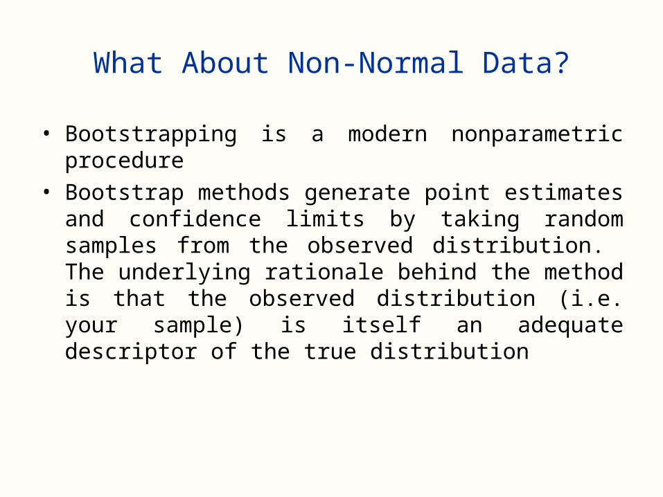
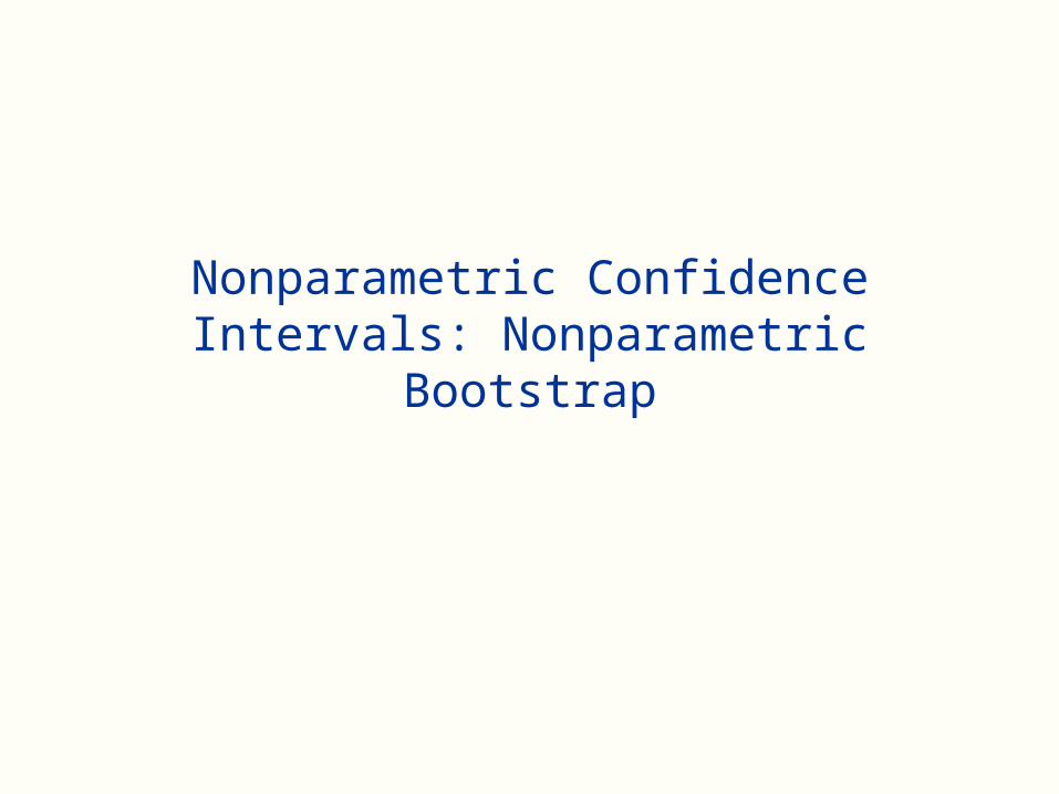
What About Non-Normal Data?

• Bootstrapping is a modern nonparametric procedure

• Bootstrap methods generate point estimates and confidence limits by taking random samples from the observed distribution. The underlying rationale behind the method is that the observed distribution (i.e. your sample) is itself an adequate descriptor of the true distribution

Non-Normal Data…

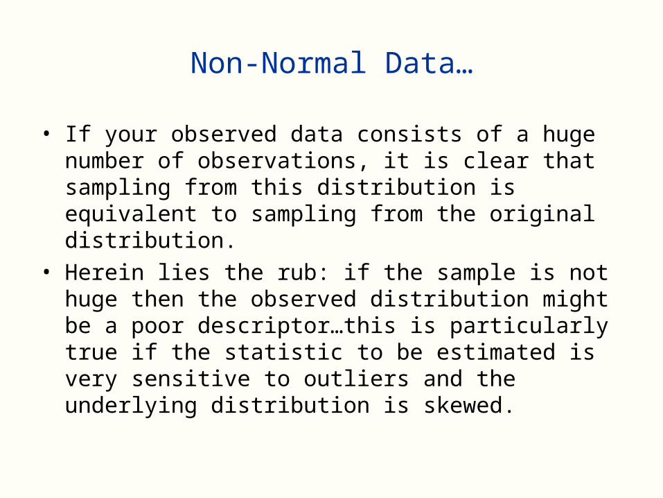
• If your observed data consists of a huge number of observations, it is clear that sampling from this distribution is equivalent to sampling from the original distribution.

• Herein lies the rub: if the sample is not huge then the observed distribution might be a poor descriptor…this is particularly true if the statistic to be estimated is very sensitive to outliers and the underlying distribution is skewed.

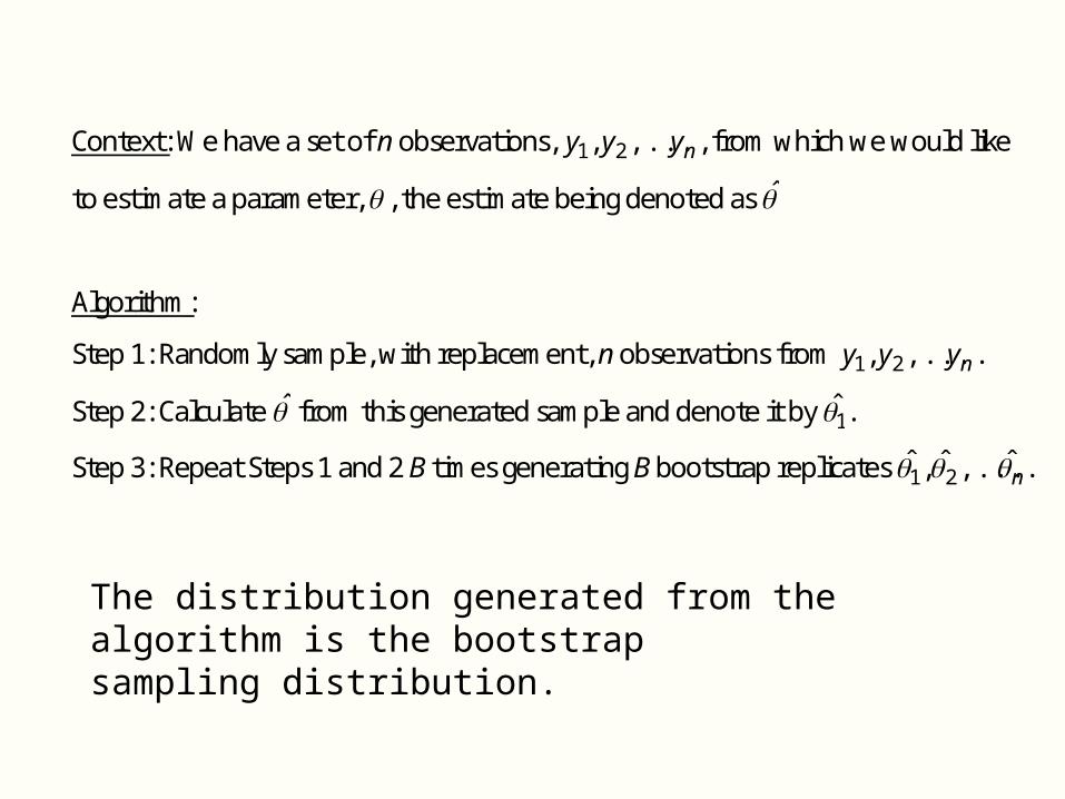
Context: We have a set of n observations, nyyy ,...,, 21 , from which we would like

to estimate a parameter, , the estimate being denoted as ̂

Algorithm:

Step 1: Randomly sample, with replacement, n observations from nyyy ,...,, 21 .

Step 2: Calculate ̂ from this generated sample and denote it by 1̂ .

Step 3: Repeat Steps 1 and 2 B times generating B bootstrap replicates n ˆ,...,ˆ,ˆ21 .

The distribution generated from the algorithm is the bootstrapsampling distribution.

The Rock Wren is a rare, threatened native bird in NZ

Ian Westbrooke provided the data from Murchison Mountains in Fiordland National Park

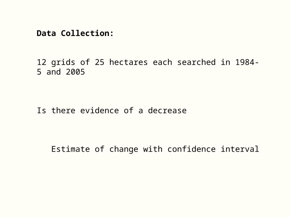
Data Collection:

12 grids of 25 hectares each searched in 1984-5 and 2005

Is there evidence of a decrease

Estimate of change with confidence interval

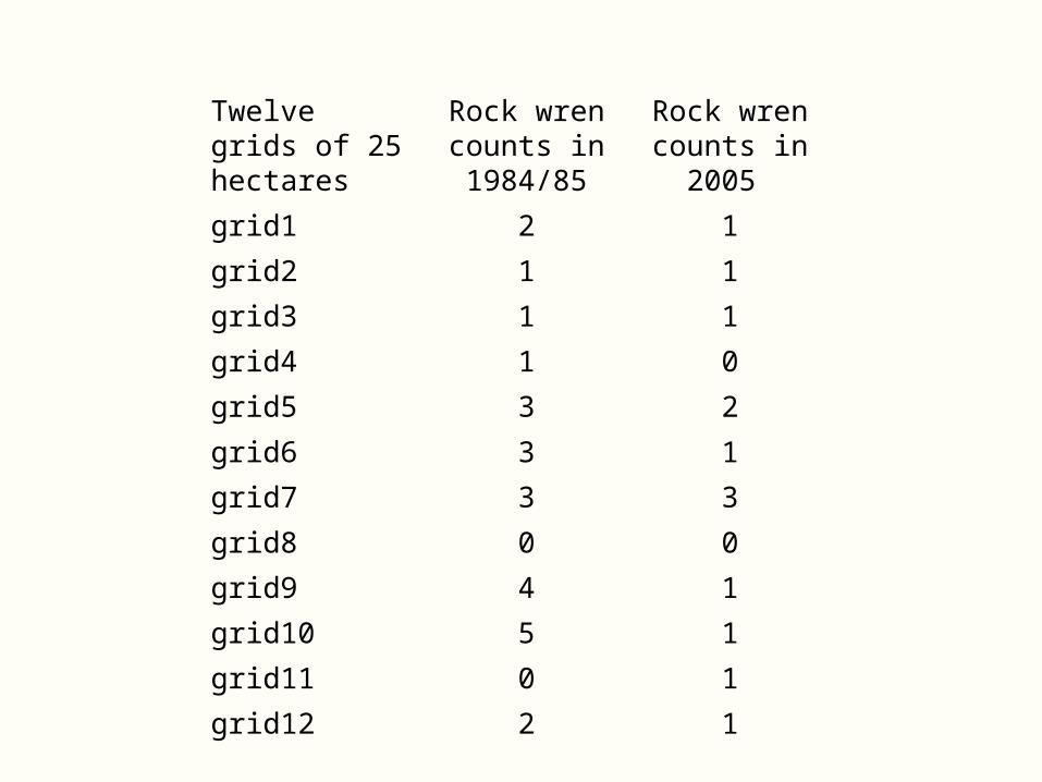
Twelve grids of 25 hectares

Rock wren counts in 1984/85

Rock wren counts in

2005

grid1 2 1

grid2 1 1

grid3 1 1

grid4 1 0

grid5 3 2

grid6 3 1

grid7 3 3

grid8 0 0

grid9 4 1

grid10 5 1

grid11 0 1

grid12 2 1

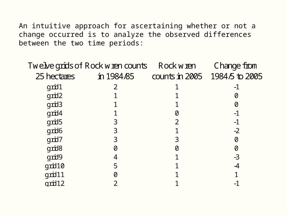
An intuitive approach for ascertaining whether or not a change occurred is to analyze the observed differences between the two time periods:

Twelve grids of 25 hectares

Rock wren counts in 1984/85

Rock wren counts in 2005

Change from 1984/5 to 2005

grid1 2 1 -1grid2 1 1 0grid3 1 1 0grid4 1 0 -1grid5 3 2 -1grid6 3 1 -2grid7 3 3 0grid8 0 0 0grid9 4 1 -3grid10 5 1 -4grid11 0 1 1grid12 2 1 -1

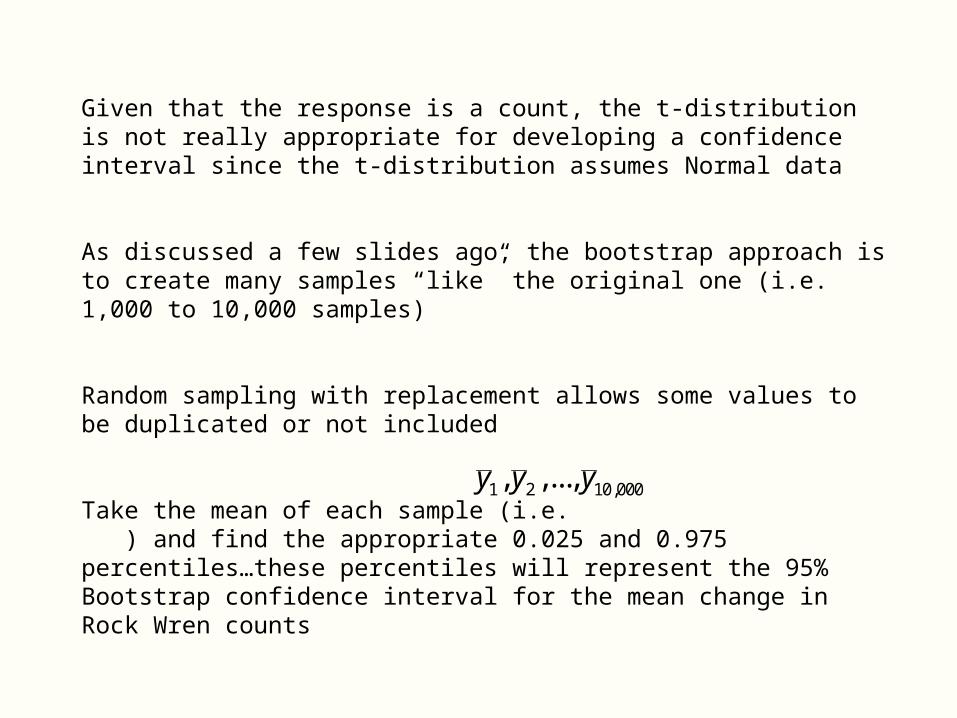
Given that the response is a count, the t-distribution is not really appropriate for developing a confidence interval since the t-distribution assumes Normal data

As discussed a few slides ago, the bootstrap approach is to create many samples “like” the original one (i.e. 1,000 to 10,000 samples)

Random sampling with replacement allows some values to be duplicated or not included

Take the mean of each sample (i.e. ) and find the appropriate 0.025 and 0.975 percentiles…these percentiles will represent the 95% Bootstrap confidence interval for the mean change in Rock Wren counts

1 2 10,000, ,...,y y y

The following function in R bootstraps a sample of data ‘B’ timeswith sample size ‘sampsize’ and computes both the mean and median of each of the boostrap samples:

bootf <- function(pop,sampsize,B){meanvec <- 1:Bmedvec <- 1:Bfor (i in 1:B){samp <- sample(pop,sampsize, replace=TRUE)mnsamp <- mean(samp)meanvec[i] <- mnsampmdsamp <- median(samp)medvec[i] <- mdsamp} # end of i loopreturn (list(meanvec,medvec))

} #end of function bootf

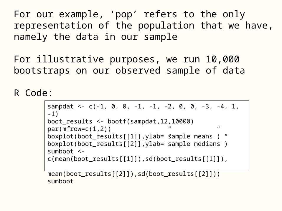
For our example, ‘pop’ refers to the only representation of the population that we have, namely the data in our sample

For illustrative purposes, we run 10,000 bootstraps on our observed sample of data

R Code:

sampdat <- c(-1, 0, 0, -1, -1, -2, 0, 0, -3, -4, 1, -1)boot_results <- bootf(sampdat,12,10000)par(mfrow=c(1,2))boxplot(boot_results[[1]],ylab=”sample means”)boxplot(boot_results[[2]],ylab=”sample medians”)sumboot <- c(mean(boot_results[[1]]),sd(boot_results[[1]]), mean(boot_results[[2]]),sd(boot_results[[2]]))sumboot

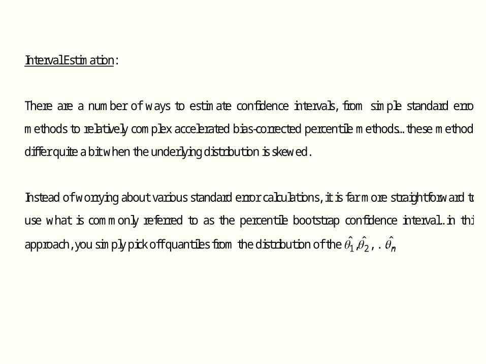
Interval Estimation:

There are a number of ways to estimate confidence intervals, from simple standard error

methods to relatively complex accelerated bias-corrected percentile methods…these methods

differ quite a bit when the underlying distribution is skewed.

Instead of worrying about various standard error calculations, it is far more straightforward to

use what is commonly referred to as the percentile bootstrap confidence interval…in this

approach, you simply pick off quantiles from the distribution of the n ˆ,...,ˆ,ˆ21

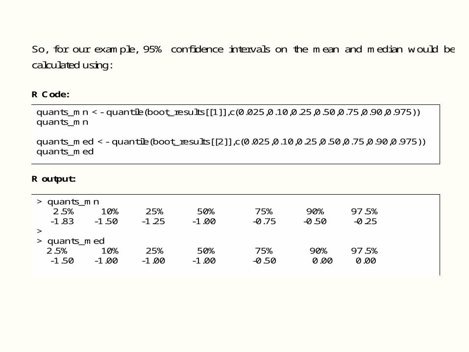
So, for our example, 95% confidence intervals on the mean and median would be

calculated using:

R Code:

R output:

quants_mn <- quantile(boot_results[[1]],c(0.025,0.10,0.25,0.50,0.75,0.90,0.975)) quants_mn quants_med <- quantile(boot_results[[2]],c(0.025,0.10,0.25,0.50,0.75,0.90,0.975)) quants_med

> quants_mn 2.5% 10% 25% 50% 75% 90% 97.5% -1.83 -1.50 -1.25 -1.00 -0.75 -0.50 -0.25 > > quants_med 2.5% 10% 25% 50% 75% 90% 97.5% -1.50 -1.00 -1.00 -1.00 -0.50 0.00 0.00

Estimating Ratios and Totals With an Auxilliary

Variable

Estimating Ratios and Totals

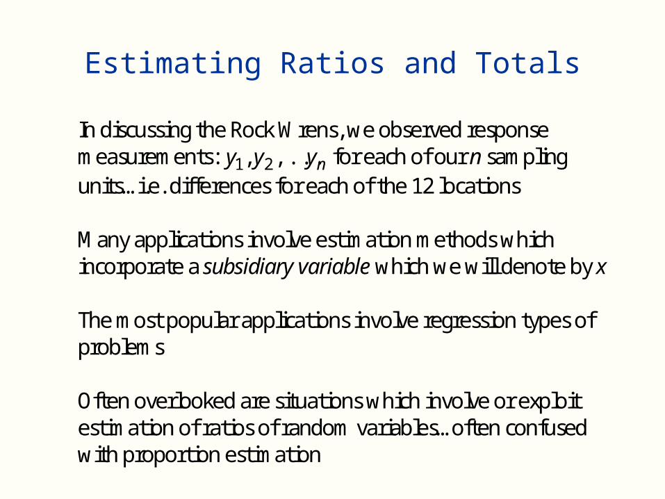
In discussing the Rock Wrens, we observed response measurements: nyyy ,...,, 21 for each of our n sampling units…i.e. differences for each of the 12 locations Many applications involve estimation methods which incorporate a subsidiary variable which we will denote by x The most popular applications involve regression types of problems Often overlooked are situations which involve or exploit estimation of ratios of random variables…often confused with proportion estimation

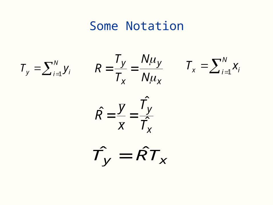
Some Notation

N

i iy yT1

N

i ix xT1

x

y

x

y

N

N

T

TR

x

y

T

T

xy

R ˆ

ˆˆ

xy TRT ˆˆ

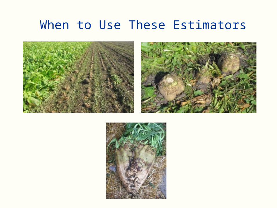
When to Use These Estimators

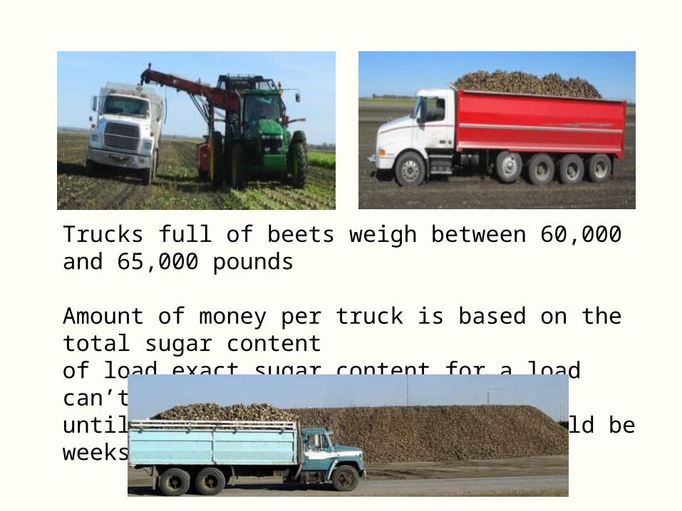
Trucks full of beets weigh between 60,000 and 65,000 pounds

Amount of money per truck is based on the total sugar contentof load…exact sugar content for a load can’t be determineduntil the extraction process…this could be weeks later

What we can compute…

1. Sugar content for a few beets…so get a sample of beets from a rancher’s field and measure sugar for each beet:

nyyy ,...,, 21 2. Next, record the weights of each of the beets selected: nxxx ,...,, 21 3. We now can compute y = average sugar content per beet, x= average

weight of each beet, and we can measure the total weight of the truck, x .

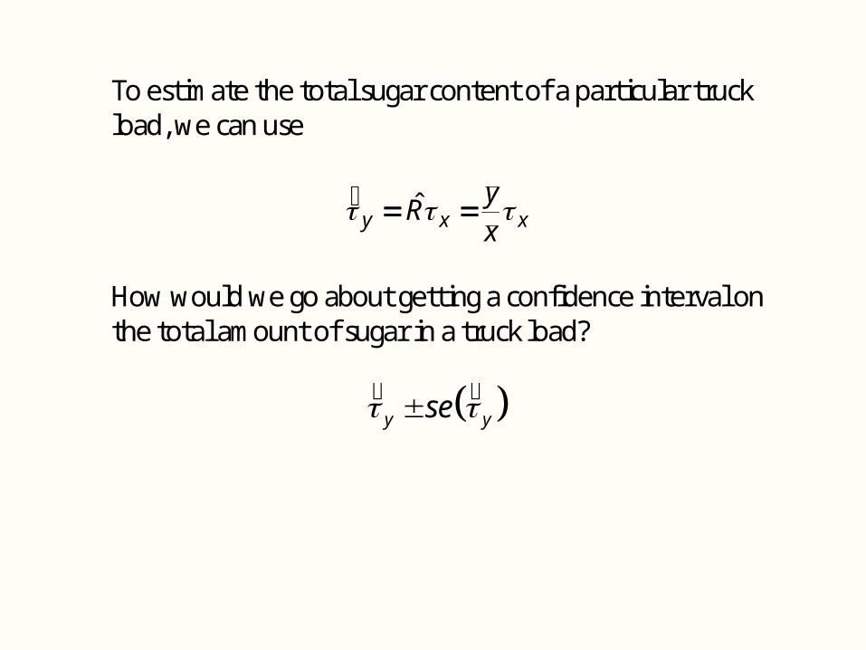
To estimate the total sugar content of a particular truck load, we can use

xxy xy

R ˆ

How would we go about getting a confidence interval on the total amount of sugar in a truck load?

y yse

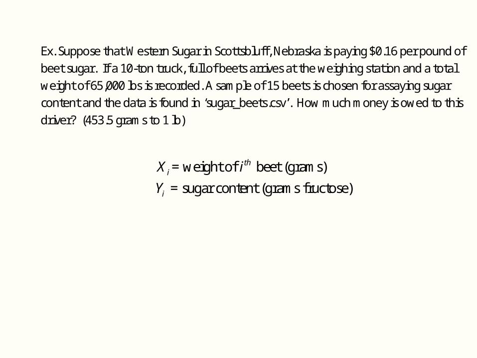
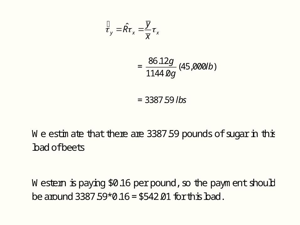
Ex. Suppose that Western Sugar in Scottsbluff, Nebraska is paying $0.16 per pound of beet sugar. If a 10-ton truck, full of beets arrives at the weighing station and a total weight of 65,000 lbs is recorded. A sample of 15 beets is chosen for assaying sugar content and the data is found in ‘sugar_beets.csv’. How much money is owed to this driver? (453.5 grams to 1 lb)

= weight of beet (grams)

= sugar content (grams fructose)

thi

i

X i

Y

ˆ

86.12 = (45,000 )

1144.0

= 3387.59

y x x

yR

x

glb

g

lbs

We estimate that there are 3387.59 pounds of sugar in this load of beets

Western is paying $0.16 per pound, so the payment should be around 3387.59*0.16 = $542.01 for this load.

How do we get a confidence interval on the total amountof sugar on this truck?

Standard error formulas exist for this type of problem BUTthey rely on lots of assumptions…bootstrapping can bea viable alternative here.

How do we go about writing a bootstrap algorithm forobtaining the confidence interval?

A few important notes on this type of use of an auxiliary

variable:

1. Commonly used when the auxiliary variable is a variable which is easily measured on the whole population (i.e. weight of beets) while the response variable is harder to measure and is obtained only from a SRS of the population

2. Useful when i iy rx are “small”…if i iy rx , then there is a linear relationship between y and x through the origin

Ex. Beet of no weight has no sugar

3. Always examine the relationship between x and y via a scatterplot

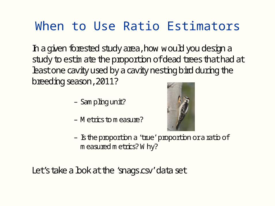
When to Use Ratio Estimators

In a given forested study area, how would you design a study to estimate the proportion of dead trees that had at least one cavity used by a cavity nesting bird during the breeding season, 2011?

– Sampling unit?

– Metrics to measure?

– Is the proportion a ‘true’ proportion or a ratio of measured metrics? Why?

Let’s take a look at the ‘snags.csv’ data set

Quadrat Num_Snags Num_Success_Snag Prop_Used1 2 1 0.52 4 2 0.53 1 1 14 2 2 15 3 2 0.666666676 4 3 0.757 4 4 18 2 2 19 0 0 #DIV/0!

10 2 2 111 4 3 0.7512 5 3 0.613 2 2 114 5 4 0.815 1 1 116 1 1 117 7 5 0.7142857118 6 4 0.6666666719 4 4 120 1 1 1

Totals 60 47 0.78333333

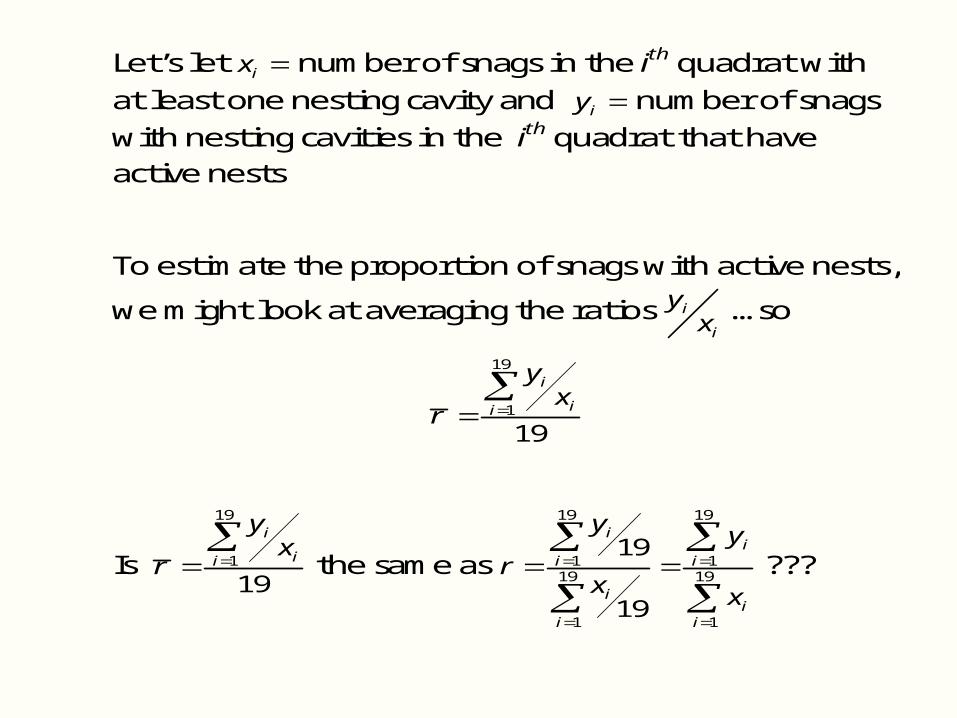
Let’s let ix number of snags in the ith quadrat with at least one nesting cavity and iy number of snags with nesting cavities in the ith quadrat that have active nests

To estimate the proportion of snags with active nests,

we might look at averaging the ratios i

i

yx …so

19

1

19

i

ii

yx

r

Is

19

1

19

i

ii

yx

r

the same as

19 19

1 119 19

1 1

19

19

ii

i i

ii

i i

y yr

x x

???

Mean of ratios is NOT the same as ratio of means

In this example,

19

1 0.83919

i

ii

yx

r

whereas

19 19

1 119 19

1 1

19 470.783

6019

ii

i i

ii

i i

y yr

x x

For this particular problem, r is the estimator that you are interested in because we are not particularly interested in this proportion at the sampling unit level…there is nothing special about the sampling units themselves

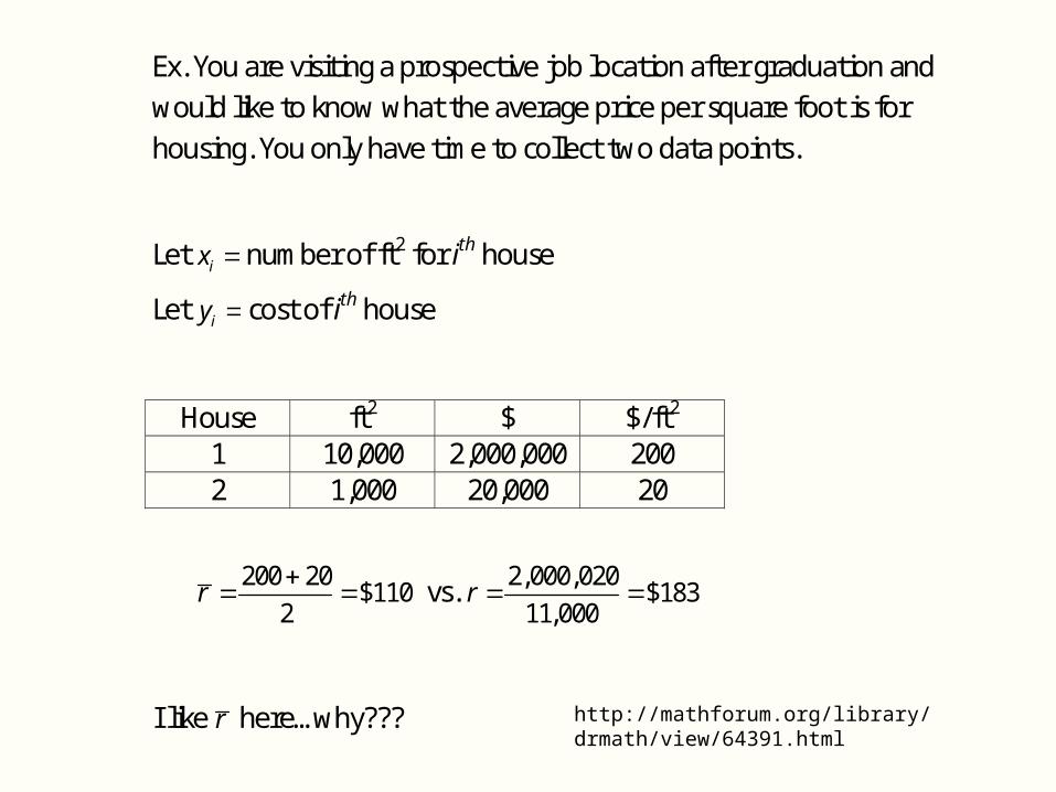
Ex. You are visiting a prospective job location after graduation and would like to know what the average price per square foot is for housing. You only have time to collect two data points.

Let ix number of ft2 for ith house

Let iy cost of ith house

House ft2 $ $/ft2

1 10,000 2,000,000 200 2 1,000 20,000 20

200 20$110

2r

vs. 2,000,020

$18311,000

r

I like r here…why??? http://mathforum.org/library/drmath/view/64391.html

The interpretation of r involves the cost per ft2 of the average house but the interpretation of r is the cost of an average ft2.

What pulls the value of r higher is the fact that the bigger house had the bigger price per square foot…since we counted each ft2 equally, the numerous high priced ft2 overshadowed the lower cost ft2

The computation of r treats all 10,000 of the expensive ft2 equally with the mere 1,000 ft2, so the smaller house pulled the average down.

Its important to note that both numbers, r and r are potentially meaningful…both are reasonably called “average cost per square foot” but which is more meaningful depends upon how you want to use it. One might be interested in the average price per square foot of floor space in the entire area…in this case, r is what you would be interested in How would you go about obtaining a confidence interval on r ? What is the difference between r and p̂ ?