MACROECONOMICSecondse.org/wp-content/uploads/2016/01/Macro-Reading1-Keynes... · the central bank...
40
MACROECONOMICS Imperfections, Institutions 8 Policies Wendy Carlin David Soskice INDIAN EDITION
-
Upload
duongquynh -
Category
Documents
-
view
214 -
download
1
Transcript of MACROECONOMICSecondse.org/wp-content/uploads/2016/01/Macro-Reading1-Keynes... · the central bank...

MACROECONOMICS Imperfections Institutions 8 Policies
Wendy Carlin David Soskice
INDIAN EDITION
Aggregate Demand2 Aggregate Supply and Business Cycles
This chapter begins the process of setting out the short- to medium-run macro model The fnst aim of the chapter is to explain how the level of output and employment is determined by the level of aggregate demand in the short run-Leo when wages and prices are sticky This provides a model of the business cycle ie how the level of output and employment fluctuates in response to changes inaggregate demand We begin with the standard approach of introducing the goods market equilibrium and then the money market equilibtium in the ISLM model The IS refers to the goods market and the LM
to the money market There are two broad ways of thinking about how monetary policy is implemented by governments or central banks and hence about the usefulness of the LM analysis On the one hand the government or central banllt can be modelled as implementing monetary policy through its control over the level or the growth rate of the money supply We shall see that this approach is best handled using the LM On the other hand the government or central bank can be seen as setting the interest rate so as to stabilize the economy and steer it toward an inflation target This is the so-called monetary rule (MR) approach developed in Chapter 3
Given the increasing prevalence of monetary rules in monetary policy-making the question arises as to why should we bother with presenting the LM analysis at all
bull First if we are to understand why governments and central banks have moved toward the use of monetary rules it is useful to have a sound understanding of the LM approach as a benchmark Moreover even if the central bank is using the MR approach theLM still exists since it represents equilibrium in the money market
bull Second the LM approach is helpful in analysing problems of deflation-Leo when prices are falling in the economy Even if the central bank uses a monetary rule to adjust the interest rate to achieve an inflation target we need to understand the circumstances under which this may be ineffective An important example is the situation where the nominal interest rate is close to zero and the economy is characterized by a falling price levelas has characterized theJapanese economy for nearly a decade
bull Third as we shall see in Chapter 9 much open economy analysis is conducted using the ISLM modeL
All three reasons suggest that even if the LM is less relevant for practical policy analysis than was once thought it remains a useful modelling tool The ISjLM model can be used
28 me MACROECONOMIC MODn
for anaJysing the deterrnirwnts of output in the short run when the government controls the money supply It also provides components that are useful later on We shall see that the lS curve is a key part of the 3middotcquation IS-PC-MR macro model developed in Chapter 3 for use with a monetary rule
In the second part of this lthaptel the focus shifts from aggregate demand to aggregate supply As we shall sec in the medium run wages and prices respond to changes in the level of activity (ie to changes in output and employment) The second task of the chapshytcr is therefore to pin down the determinants of the medium-run level of employment at which the labour market is in equilibrium and pressures for wages and prices to change are absent The integration of the short- and medium-run components is introduced in the final section of the chapter through the use of the aggregate demand and aggregate supply framework
We contrast the explanation of business cycle fluctuations based on shifts in aggregate demand in the presence of sticky wages and prices on which we concentrate in this book with a completely different one where it is shifts on the supply side of the economy such as technological change that produce booms and recessions This second approach is called the Real Business Cycle model
1 Aggregate demand
To understand how the level of output is determined in the short run we look for the sources of changes in the aggregate demand for output The short run is defined here as the period during which prices and wages are given There are a number of ways of explaining why prices and wages might not respond immediately to changes in demand Institutional arran~ements normally mean that wages are reviewed periodically and not continuously Acommon argument in support of price stickiness is that there are costs associated with changing prices which are referred to as menu-costs It is also useful to remember that it is profitable for firms in imperfectly competitive markets to increase output in response to higher demand even if the price remains unchanged For the moment we just assume that wages and prices are sticky-they do hot respond to changes in employment or output in the short run A more detailed discussion of the implications of price and wage behaviour for macroeconomics is presented in Chapter 15 The following terms are used by different authors to refer to this assumption nominal rigidity sticky wages prices fix-price
The standard model that is used to summarize the way in which the level of output is determined by aggregate demand in the short run (ie with sticky wages and prices) is the ISLM modeL1 It consists of two parts the goods market and the money market We think of a short-run eqUilibrium in the economy as a situation in which both the goods and the money market are in equilibrium The goods market part is labelled IS after the Investmen t-Savings version of the goods market eqUilibrium condition planned investshyment must be equal to planned savings for equilibrium in the goods market The money
1 The model was introduced by John Hicks in 1937 (Hicks 1937) For a concise and interesting discussion of its origins and impact see Lrijonhufvud (1987)
SUIPty tND BUSINESS CYCLES 29
market part is labelled LM after Ih( equality between rnoney demand (L-iquidity) and Money supply when the money market is itl equilibrium In ISILM equilibrium the level of output (and employment) and 11)( interest )at( lJre constant
The model is useful I)(middotcausc it allows us to work out what happens to output and to the interest rate when there is a change in aggregate dernand or when the government changes its polIcies On the IS side we can analyse
bull shifts in consumption or investment
bull changes in fiscal policy Le in government expenditure or taxation
On the LM side we can analyse
bull shifts in money demand
bull changes in monetary policy eg in the money supply
2 The goods market the IS curve
The IS curve shows the combinations of the interest rate and output level at which there is equilibrium in the goods market For goods market equilibrium the aggregate demand for goods (and services) must equal the supply Since we assume that wages and prices are fixed the supply of output will adjust to any change in aggregate demand
Aggregate demand refers to the planned real expenditure on goods and services in the economy as a whole Equilibrium requires that planned real expenditure on goods and services is equal to real output
(goods market equilibrium)
where yO is planned real expenditure and y is real output Aggregate demand is made up ofplanned expenditure onconsumption and investment
by the private sector and planned government spending It can be written as
yD c(y t wealth) + J(r A) +g (aggregate demand)
where C is consumption J is investment andg is government spending all in real terms t is total taxation r is the real rate of interest and A refers to other (non-interest rate) determinants of investment In general we use lower case letters to refer to real variables and upper case ones to refer to nominal variables so y is real output and Y is output in money terms (eg in euros or dollars) However this is not always possible we use i for the nominal interest rate and I for real investment
Some important features of the short-run macroeconomic model can be shown most easily ifwe assume linear functions We shall use a simple linear consumption function thatsays consumption is a function of current post-tax (ie disposable) income and other factors such as wealth that are summarized in a term labelled autonom(ms consumption which is assumed to be constant
C = Co + Cy(y - t) (consumption function)
)0 THE MACROECONOMIC MODEl
where en is (lutonOlllOtl$ consumption and cj is the constant proportion of current disposable income that is consurned 0 ( cj 1 The term cj is called the marginal propensIty to consume out of disposable income Disposable income is income minus taxation (y t) t is the total tax HVeI1Ue and if we taklgt ulincar tax function then
(tax function)
where 0 lt t) 1 Thus if we substitute the tax function into the consumption function and rearrang(~ the terms the consumption function is
C Co + c) (J Iy )y
A notable feature of this consumption function is that consumption is affected by the current level of activity in the economy In Chapter 7 we look at the microfoundationsof consumption behaviour to see why current and expected tJiure income are likely to be relshyevant for consumption expenditure The Simplest way to incorporate the inSights of the forward-looking model of consumption is by including in Co thedeterminants of expected future income The consumption function shifts when expected future income changes The empirical evidence discussed in Chapter 7 confirms that current and expectedfuture income inJ]uence current consumption
Investment is assumed to depend negatively on the reallate of interest and positively on expected future profitability the determinants of which areproxied by the termA The simple idea is that firms are faced with an array of investment projects which are ranked by their expected return If the interest rate falls then this reduces the cost of capital and makes some projects profitable that would not otherwise have been undertaken Similarly if the expected return on projects rises (because there is a surge of optimism in the economy) then at any given interest rate more projects will be undertaken We can write this investment function
1= I(rA) (investment)
It is sometimes handy to use a linear form I = A ar where a is a constant Expectatiorial or confidence factors are often considered crucial determinants of investment behaviour This would imply that shifts of the investment function arising from changes in A could be of greater significance than movements along the investment function in response to interest rate changes A deeper examination of investment behaviour based on microshyeconomic foundations is to be found in Chapter 7
The IS curve is defined by the goods market equilibrium condition (fP = y) To derive an explicit form for the IS curve we use the linear versiqns of the consumption and investment functions and substitute them into the planned expenditure equation
(planned expenditure)
The planned expenditure equation is then substituted into the goods market eq uilibrium condition We rearrange using the fact that in the goods market equilibrium)1) y and replacing (1 cy) by the marginal propensity to save Sy to define an equilibrium locus of
AND lWSINIESS CYClES 31
combinations of the interest rate and output
~ e)i [co -+ (A ar) +gj
1 -Ico --1- (A ar) 1shysF -+ C)lt ---v---
multipl ier
The IS curve states that for a given interest rate the level of investment is fixed to this level of investment is added autonomous consumption and government spending and the associated level of output is found by multiplying the sum by the constant S)-1C
y l
which is known as the multiplier Savings and taxation both represent leakages from the feedback from income to expenditure The reason that the tax leakage (ty) is multiplied by cy is that only that part of tax revenue that would have been spent constitutes an extra leakage over and above savings The IS curve is downward sloping because a low interest rate generates high investment which will be associated with high output By contrast when the interest rate is high investment and hence equilibrium output is low
The IS curve is derived graphically in Fig 21 At rH investment (10 A arH)
autonomous consumption and government spending are shown Multiplying 10 +Co +go by the multiplier gives output equal to planned expenditure Yo on the IS curve Using the same logic at a low interest rate planned expenditure will be high owing to high investment Goods market equilibrium dictates a correspondingly high output level
Investment function
Investment plus autonomous consumption and government spending
((r
1--shy
I I
10 Yo yl
Note that lo=A -a -Hand It=A amiddot TL
Figure 21 Deriving the IS curve
32 n~E MAClWECONOIVIlC MODEl
Using the IS curve equation and 11le diagram we can separate the deterlllinants of the slope and position ofthe lS curve into three groups
(1) Any change in the size of the multiplier will change the slope of the IS curve For example a rise in the proP(gtnsity to consume will increase the multiplier making the IS flatter it rotates counterclockwise from the intercept on the vertical axis
(2) Any ch~nge in the interest sensitivity ofinvestment (a) will lead to a consequential change in the slope of the IS curve a less interest-elastic investment function will be rellected in a steeper IS curve
(3) Any change in autonomous cOl1swnptiol1 or in government expenditure (co g) will cause the IS curve to shift by the change in autonomous spending times the multiplier A change in the variable A in the investment function also shifts IS2
Policy can be used to manipulate the IS curve through channels 1 and 3 For example if income tax is proportional ie if t = ty)l a lower tax rate increases the size of the multiplier and as in 1 above swings the IS to the right making it flatter Any change in government spending will shift the IS in the manner described in (3) above
A feature of the IS model of the goods market is that quantities adjust through the multiplier process to take the economy to a stable short-run equilibrium For example a fall in planned investment leads to a multiple contraction of output and employment until the level of income has fallen to the extent required to make saving equal to the lower level of investment Initially income falls by the fall in investment fI As the result of the fall in income and assuming ty = 0 consumption declines by fc = cyfI
This fall in consumption in tum reduces income and in the next round consumption falls once more fc = cy(cyfl) = cfI To calculate the total drop in income we sum the series3
fy = fI + cyfI + cfI + c~fI + = (1 + cy + c + c~ + )fI
1=--middotfI
1 - cy
= ~ fI = multiplier x fI Sy
The change in output is equal to the multiplier (Le 1jsy) times the change in investment
2 In the Appendix to this chapter we show how the statements 1-3 can be made precise in the case of linear functions by working through the algebra and geometry of the IS curve
3 This is the sum of a geometric series We want to find an expression for the series 1 + Cy + c + c)~ + which we call x If we put
X = 1 + Cy + Cy 2 + Cy
3 + (21) then
Cy x = Cy + Cy 2 + Cy
3 + (22) and if we subtract 22 from 21 we have
x(l-cy)=l
1 =gtx=--
1 - cy
AND BUSINESS (leugt 33
r Excess supply of goods yf) lt co )J
1 x
z
Excess clernand for goods yOgt YYI
IS
Figure 22 Adjustment to goods market equilibrium excess demand at point X leads to a rise in output excess supply at point Z leads to a fall in output
Another way of focusing on quantity adjustment to a new goods market equilibrium is to characterize positions off the IS curve (Fig 22) At pOint X with output Yx to the left of the LS curve there is excess demand in the goods market because at the interest rate rl planned expenditure is equal to Yl With aggregate demand in excess of output stocks will fall and output will rise until Y = yD on the IS curve
3 The nloney market the LM curve
The LM curve represents the combinations of the interest rate and output at which the money market is in equilibrium so the focus here is on the way the money market works Throughout the chapter it is assumed that the central bank controls the money supply-~we model central banks using an interest rate based monetary rule in Chapter 3
31 Demand for money
A common confusion that arises when first studying macroeconomics is between the decision to save and the decision to hold money The decision to save refers to the use that is made of the flow of income Of the income received in any given period (eg a month) from working and from other sources such as interest income there is a proportion that is saved and a proportion that is consumed If consumption exceeds income then the individual is dissaving-Le they are borrowing and accumulating debts
What then is the demand for money Whereas the saving decision is an income allocation decision the demand for money is a decision about the form in which to hold your wealth Should you hold it as money or as another asset To answer this it is necessary to know the difference between money and other assets When someone asks how much money you have you might answer by counting the notes or coins in your wallet or you
34
might include the balance in your cheque account because you havtinstant access to this money by writing a cheque or using a debit G1H1You luigl1t also add in the balances on your 0111(1 higher illter(sl bank accotll1ts~the term accounts for which you have to give a certain notice period if you want to withdrnw money witbout a penalty All of these are money and they range from a narrow definition (notes and coins) to a broad one (term deposits) As we move from narrow to broad money there is a gain in the interest return and a loss in liquidity
Note that throughout the discussion of money demand and money supply the relevant interest ratt~ is the nominal interest rate i One characteristic common to all forms of money is that it is a very or fairly liquid asset and therefore indispensable for carrying out transactions in the economy Second if you have eurol 000 in your account then as long as you do not withdraw any of it the value in money terms does not fall This means that money is capital-safe in nominal terms If the money is in an interest bearing account then the nominal amount will rise as interest accrues
311 Money and bonds
Although some forms of money do pay interest there are other assets available in the economy that offer a higher return than a term deposit as long as you are prepared to take on some risk In addition to supplying money the government can borrow from the general public by selling government bonds The key difference between government bonds and money is that bonds are not capital-safe in nominal terms if there is a rise in the rate of interest then the market value of the bond falls
To understand the inverse relationship between the market price of a bond and the interest rate consider a bond that is issued by the government at a face value of euro100 and that pays euro5 per annum in perpetuity If the market interest rate is 4 then the price the bond will sell for in the market (the market price) will be such as to make the yield of euro5 represent a market return of 4 The market value of the bond will be where O04x = 5 Le x = 5004 = euro125 An interest rate lower than 5 implies a market value higher than the face value of the bond If the interest rate is even lower at say 2 then x 5002 euro250 and similarly if the interest rate is higher at say 8 then the market value is euro6250 There is an inverse relationship between the market value of the bond (Ie the price at which it will sell in the market) and the market interest rate It is clear that only if the interest rate is 5 is the market value of the bond exactly equal to its face value So unlike euro100 in cash the nominal market value of a euro100 bond will go up whenever the nominal interest rate falls and vice versa
312 Demand for money versus bonds
Consider the choice between holding ones assets in the form of money or in bonds for example from the perspective of a business deciding how to manage its cash (As we shall see in Chapter 8 the discussion is not fundamentally different when additional assets such as equities are introduced) Money is needed in order to carry out transactions in a market economy Since desired transactions vary with the level of income so will the demand for money But the cost of holding assets in the form of money is that interest income is foregone A rise in the interest rate will shift the balance of advantage in favour of interest-bearing assets including bonds
I)f~MANI) SUPPIV AND BUSiNESS CYClES 35
We can summarize the demand for lnoney as follows
(demand for money)
where i is the nominal interest rate We return to the question of the difference between the real interest rate r that features in the 15 equation and the nominal interest i that features in the money market We are dealing here with the iL part of the LM where the tU refers to the demand for liquidity A rise in the level of income holding the intershyest rate unchanged will raise the demand for money (ie aLlaygt 0) and a rise in the interest rate holding the level of income unchanged will lower the demand for money (ie DLlai lt 0) Note that the demand for money is expressed in real terms ie (MIP) since it is normally assumed that a rise in the price level wiil raise the nominal demand for money in proportion
Just as in the analysis of the goods market it is sometimes helpful to express the demand for money as a linear function of the level of income and the interest rate
(demand for money)L(y i) =
asset demand trltmsactions demand
where I VT and Ii are positive constants The term (1 Iii) reflects the asset motive for holding money and the term y) reflects the transactions motive for holding money In the famous theory called the Quantity Theory of Money the only determinant of the demand for real money balances is the level of output In other words only the
transactions motive is present The Quantity Theory of Money can be stated as ~D =
t y where v is the constant velocity of circulation We use the now standard more general demand for money function in which the transactions demand is only one part of the demand for money Hence although the transactions velocity VT is constant the overall relationship between money demand and output is not it will vary with changes in the interest rate
313 Asset and speculative motives
Two of the explanations given for the inverse relationship between the demand for money and the interest rate are known as the asset motive and the speculative motive Both relate to the choice between holding money and bonds Keynes argued for the relshyevance of the speculative motive as follows if an individual believes that the current interest rate is above the level she considers normal then she will expect the interest rate to fall to normal in due course Under these circumstances she will choose to hold finanshycial assets over and above the money required for transactions in the form of bonds She doesthis because she will expect to reap a capital gain on the bonds when the interest rate falls to its normal level The converse would be true for a current interest rate believed to be below normal Keynes believed that the subjective assessment of the normal interest rate would vary across the population producing a smooth inverse relationship between the interest rate and the aggregate demand for speculative balances Moreover a central implication of Keyness argument is that expectations drive financial markets and that
36 rifE MACROECONOMIC MODEl
shifts in expectations have a self-fulfilling character If bondholders suddenly believe that the interest rate will be higher in the future than they had previously believed they will exptct capital losses and will sell their bonds driving bond prices down and interest rates up~the expectation of a rise in the interest rate is fulfilled This feature of financial markets is of great importance for monetary policy
A more general rationale for the negative dependence of the demand for money on the interest rate was developed by James Tobin in 1958 Instead of assuming as had Keynes that each individual is certain about what she expects the future rate of interest on bonds to be Tobin focused on the implications of investor uncertainty In the simplest version of Tobins model risk-averse4 individuals allocate their POlifolio between a riskless asset that pays no interest (money) and a risky one with a positive expected return (bonds) The individuals utility depends positively on the return from holding the asset and negatively on the risk ofholding it To maximize utility the individual will hold a mixture of the two assets trading off the benefits of a higher expected return against the aSSOCiated risk according to her own preferences A higher interest rate would lead her to substitute bonds for money (reduce the demand for money) because the higher expected return would offset the additional risk incurred This produces an inverse relationship between the demand for money and the interest rate A more detailed discussion of the speculative and asset motives can be found in Chapter 8
32 Money market equilibrium
Money market eqUilibrium requires the demand and supply of money to be equal
M SMD (money market equilibrium) p p
money demand = money supply
where the demand for money depends on the nominal interest rate and the level of output as defined above and the supply of money is assumed to be fixed by the monetary authorities at MS In Chapter 8 we examine critically the assumption that the monetary authority can fix the supply of money for now we assume that this is possible This assumption allows us to develop a useful benchmark modeL If we substitute the demand for money function and the fixed money supply into the equilibrium condition
MS L(y i) = P (money market equilibrium)
we can define an upward sloping locus of money supply equal to money demand equilibria~the LM curve in the interest rate-output diagram
The upward-sloping LM curve can be explained as follows At a low level of income the transactions demand for money is low because less money has to be held to finance
4 Someone is risk averse if when offered a fair bet would refuse it ie if offered the choice between receiving euro100 with certainty or the chance of euro200 (or zero) on the outcome of the toss of a fair coin the individual would always take the certain euro100 In other words the individual prefers a certain value of euro100 to an uncertair return with an expected value of euro100
DEMJUIO SUPtV AND BUSINESS CYClES 37
transactions Since the supply of money is ftxed for supply to equal dernand in the money market there must be a correspondingly high asset (or speculative) demand for money A low interest rate will ensure thb since the returns from bondholding relative to the risks involved are low The converse argument clssociates a high income level with a high interest rates
Using a linear demand for money function there is a neat way of deriving the LM curve so that it is easy to see how shifts in tbe demand for money or changes in the interest sensitivity of the demand for money or changes in the money supply will affect the LM curve The method is shown in Fig 23 in two steps Working through this diagram is a
iiS-p(a) i
I1irst at ill the interest-sensitive demand for money (1-1 i) is low and is shown by the distance c
-------~~----__L W MD Second for -p- ==-F at lilt the distance ii is the transactions demand for money(-t-middot y)
11
Step 1 M P
(b) i
aiH +-------------
I
x
LM(~)
z I I
Step 2 Yo MyP
Figure 23 Deriving the LM curve
5 The explicit form of the LM equation using the linear demand for money function is
_1 1
1(shy MS) + 1 P 1 VT
y (LM equation)
38 TIU
good rnethod of securing your undprstanding of
bull til( transacUons (k~UHlnd for ll1()m~y and the role of Jr
bull the asset (or speculative) demand forrnoney and the role of
bull the role of the hgtvel of the money supply set by the central bank or the government AIl and
bull the equilibrium condition in the money market L ~f~
In step 1 draw in the vertical real money supply Jine6 Now draw in the interestshysensitive component of the demand for money backwards Le relative to the money supply line as shown in Fig 2 3 As we know when the interest rate is high the demand for money for asset purposes will be low (in the diagram this is the distance c) Now make use of the money market equilibrium condition ~~ Ii + i~ y For money
market equilibrium asset demand for money (7 -- ld) plus the transactions demand for
money (~ 1) are equal to the money supply Hence we can see how large the transshyactions demand for money must be for money market equilibrium at the interest rate hi in Fig 23 This is shown as the distance a Once we know the transactions demand for money that is associated with the interest rate iu ie the distance a then since VT is a constant it is straightforward to take the second step of calculating the level of output y that is consistent with generating this demand for money Yl = VI X (transacshytion demand for money at iIi) This fixes the level of output )J at which the money market is in equilibrium when the interest rate is hi point X in the bottom panel Point Y can be derived in the same way By joining points X and Y the LM curve is drawn
From the derivation of the LM curve there are four ways in which the position andor the slope of the LM curve can be affected
(1) A change in the transactions velocity ofcirculation The transactions velocity of circushylation VI is the constant reflecting the proportional relationship between income and the demand for transactions balances It is the number of units of income that one unit of transactions balances can finance Any rise in the transactions velocity as the result of financial innovation (eg introduction of credit cards development of non-bank finanshycial institutions) will rotate the LM to the right (clockwise) making it flatter
(2) A change in the interest sensitivity of the asset demand for money Ii A more interestshysensitive demand for money reflecting the fact that small changes in the interest rate will have large effects on the portfolio mix between money and bonds will produce a flatter LM curve bull A special case arises when the interest-sensitive demand for money becomes perfectly
elastic in which case the LM curve becomes horizontal The simplest interpretation of this is in terms of speculative demand if it is the case that no one believes that the normal interest rate is lower than the actual interest rate pound then the speculative demand for money is perfectly elastic at i because nobody is prepared to use spare cash
6 If you want to see what happens if the supply of money is also sensitive to the interest nlti~ you can modify the method at this pOint
DEMAJOf SUPPIV ANO BUSiNESS CYClES 39
balances to furthe Irlel up the bond price Under such conditions the interest rate Is so low that everyone belit~ves it will rise to its nornlaJ level (opinions will differ on what that l10nnaJ JeveJ is) In Pig 23 if i f th(~ intereslsensitive money demand and the LM curves would turn horizontal at it This is the famous liquidity trap case to which we return at the end of section 42 (see Fig 26)
(3) A change in the money supply An increase in the money supply will shift the LM curve to the right since at any interest rate with a given asset demand for money a higher money supply will require higher transactions balances to bring money demand into line with the higher supply A higher output level will generate the higher transactions demand
(4) A change in the price level For a given interest rate with a higher price level the available transactions balances can only finance a lower amount of output The LM curve shifts to the left
The simple mathematics and geometry of the LM curve required to specify statements 1-4 are presented in the Appendix to this chapter
At a point such as X above the LM curve in Fig 24 with the output level yo and interest rate ix money balances are too high for money market eqUilibrium We can see that the disequilibrium could be eliminated either by a rise in the level of output or by a fall in the interest rate When there is excess supply of money (excess demand for bonds) the excess money balances are channelled into the bond market the bond price is bid up and the interest rate reduced (recall the earlier discussion of the inverse relationship between the interest rate and the price of bonds) The converse situation of excess demand for money is true of a point such as Z below the LM curve This will be cleared by the sale of bonds which pushes down the bond price and raises the interest rate
LM(~)Excess supply of money
(w MD) ITgtp ~lw ~ X
I
~ ~
I
i t Excess demand of money t (W MD) jZ pltp ~l
iz
yYo
Figure 24 Adjustment to money market equilibrium excess supply of money at point X leads to a fall in
the nominal interest rate excess demand for money at point Z leads to a rise in the nominal interest rate
40 nuz MACROECONOMIC fvlODEt
4 Putting together the IS and the LM
By combining the goods and money markets the interest rate and the short-run equilib dum level of output for a given price level are determined Before that there is one tricky problem that needs to be addressed In the derivation of the IS curve it is the real interest rate r that is relevant since investment spending depends on the real rate of interest In the derivation of the LM curve it is the nominal interest rate i that is relevant since the demand for money depends on the nominal interest rate
41 Real and nominal interest rates
To clarify why it is the real rather than the nominal interest rate that affects real expenshyditure decisions in the economy think about a firm considering an investment project A higher money or nominal rate of interest will not impose a greater real burden on the firm if it is balanced by correspondingly higher inflation because the expected profits from the ill vestment project will be higher in money terms and the balance between the real cost and the real return on the project will not have changed
The real interest rate is defined in terms of goods and the nominal interest rate interms of money Thinking of a consumer good the real rate of interest r is how much extra in terms of this good would have to be paid in the future in order to have one of the goods tOday 1 good = (1 + r)goodt + 1 where the subscript t refers to today and t + 1 to one period later 1be nominal rate of interest is how much extra in euros would have to be paid in the future in order to have one euro today 1 euro (1+i)eurot-j-l If goods prices remain constant then it is clear that the real and nominal interest rates are the same if you lent one euro today you would be able to buy (1 + r) goods in the future In general
1 + r = (1 + i) P
where it is the expected price level in the future (pr+l) that cOJnesinto play since at time t we do not know what the price level will be at t + 1 If we use the following definition of expected inflation
Eif
then
P 1 1 + ifE
By rearranging the above expression it follows that
(1 ) = (1 + i)+ r (1 + ifE)
IlEMAND SUPPLY AND BUSINESS CYCUS 41
and therefore that
r
When expected inflation is low the denominator of this expression is close to 1 and we have the standard approximation for the relationship between the real and the nominal rate of interest
gt~ r + 71E
Inflation expectations will drive the divergence between the real and nominal intershyest rates It should be noted that only one of these three terms is observable the nomishynal interest rate The real interest rate can be estimated from historical data on the nomishyna) interest rate and the rate of inflation this gives a measure of the so-called ex post real rate of interest Alternatively an ex ante measure can be derived from a model that is able to predict inflation Finally if bonds have been issued in the economy that are protected against inflation because the face value is indexed by the rate of inflation then the yield on such a bond is a real rate of interest and can provide a third measure But there are only a few countries that have issued index-linked or inflation-proof bonds (UK in 1981 the USA in 1997 France in 1998)
42 The ISILM model
So as to avoid (temporarily) the problem of the IS depending on the real and the LM on the nominal interest rate we concentrate on how the ISILM model works when the real and nominal rates are identicaL This requires us to assume that inflation is zero and is expected to remain so To remind us that two different interest rate concepts are involved we draw the ISILM diagram with both I and i on the vertical axis We shall return to show how to amend the ISILM model when inflation is different from zero in Chapter 3
Now that both the IS and the LM relationships have been derived the short-run equishylibrium interest rate and level of output will be determined by the intersection of the two curves To see how the ISILM model works the initial [SILM equilibrium is disturbed by changing one of the exogenous variables First we consider the character of the new short-run equilibrium and as a second we discuss the likely adjustment ofthe economyto it The path of adjustment of the economy in the face of a disturbance will depend on the speed of adjustment in each market The most plausible simple assumption is that money market disequilibria are cleared very rapidly in relation to disequilibria in the goods and services market In the ISILM diagram this means that the economy returns to the relshyevant LM curve rapidly-the adjustment occurs through changes in the price of bonds in the financial markets and therefore in market interest rates Goods market adjustment takes place less quickly since it involves adjustments to production and employment
We look at two examples of government policy changes In the first example (Fig 25) government spending rises The new IS is IS(gd to the right of the original one The new short-run equilibrium is at the point A output is higher and so is the interest rate Higher government spending will generate higher aggregate demand and a higher output leveL
42 THE MACROECONOMIC MODEl
(a) r ~
LM(~O)
Aft
y
(b) r
LM(~)
B C
y
Figure 25 Comparative statics in the ISILM model sluggish adjustment in the goods market and rapid adjustment in the money market
(a) Fiscal pollcy rise in government spending
(b) Monetary policy rise in the money supply
Higher incomes will mean a higher demand for money but sinlte monetary policy is unchanged (ie the LM curve remains fixed) a higher interest rate will be required in the new equilibrium to dampen the asset demand for money
Let us now think about the likely process of adjustment to the new equilibrium In the first instance the rise in government spending produces excess demand for goods and results in unplanned inventory decumulation or in longer waiting times for services If the rise in demand is sustained then employment is increased The economy moves from A to B The rise in real income associated with higher output boosts the transacshytions demand for money with the result that there is excess demand for money balances
SUPPLY Alii) BiJSINESS CYClES 43
at B Bcmds are sold causing the bond price to fall and tIle jnt(~rest rate to rise (15 to C) The risc in the interest rate dnmraquocn)) til xcess demand for goods by reducing investment demand n(v(~rtheless at C there remains excess demand owing to increased consumpshytion associated with the HIU) tiplier effects of the rise in government spending Output and employm(~nt rise funIwr (C to D) The adjustment process continues until the new equishylibrium atA I is attained 1l1e full multiplier expansion of output (A to All) does not occur because when there is a flscal expansion without any change in thtgt money supply the increase in the interest rate causes a fall in interest-sensitive spending The implications of financing an increase in government expenditure by (i) taxation (ii) bond finance as in the above example and (iii) money flnance are compared using the [SILM model in Chapter 6
In the second example (Fig 25) the government or central bank increases the money supply through the qse of open market operations This means that it enters the money market purchasing bonds in exchange for newly printed money The LM
curve shifts to the right to LM(~1) Once again we first consider the new short-run equishylibrium which has a higher level of output and a lower interest rate With a higher money supply the higher demand for money in the new equilibrium will require a lower interest rate A lower interest rate will be associated with a higher level of investment and output (point AI in the lower panel of (Flg 25raquo
We tum now to the adjustment from point A to the new short-run equilibrium at AI The immediate effect of the monetary authoritys action is to create excess supply of money the implied excess demand for bonds raises bond prices and lowers the interest rate The economy moves from A to 13 immediately attaining the new money market
equilibrium along LM( 1) Tl~e fall in the interest rate creates excess demand in the goods market by stimulating investment Higher investment demand pushes up output and employment raising output from B to C At C there is once again money market disequilibrium as excess demand for money accompanies the rise in output The interest rate rises (C to D) Adjustment of output and the interest rate will continue until the new equilibrium at AI is reached
Fig 26 shows why expansionary monetary policy may not raise output even in the short run If the interest rate is i the LM curve is flat When the central bank enters the money market to purchase bonds there is no impact on the price of bonds if everyshyone believes the only direction for the interest rate in the future is up this implies they believe that bond prices will fal1 Bondholders therefore willingly sell bonds at the existshying price being indifferent between money and bonds as the prospective capital loss on bonds just offsets the interest received with the result that there is no rise in the bond price and no fall in the interest rate The economy is in a liqUidity trap where new money pumped into the economy is willingly held as money balances The central bank is thereshyfore powerless to use monetary policy to shift the economy to a higher level of output For decades the case of the liqUidity trap was viewed as a theoretical possibility with little practical relevance but the re-emergence of an era with very low nominal interest rates in the 1990s has revived interest in it Since the nominal interest rate cannot fall below zero the notion that everyone believes the interest rate will rise becomes plausible The liquidity trap plays a role in the analysis of the long]apanese slump in the 1990s and is discussed further in Chapters 5 and 17
44 THE MACROECONOMIC MODEl
y
Figure 26 The liquidity trap
5 Aggregate supply
We turn now to setting out systematically the structure of the supply side of the economy that will be used to create an integrated short- and medium-run model We begin by noting briefly how the supply side looks in a competitive model before moving to the more general model of imperfect competition with which we mainly work
51 Equilibrium in the competitive labour market
In the competitive labour market the demand for labour and the supply of labour depend on the real wage The downward-sloping labour demand curve shows the labour demanded at a given real wage With a fixed capital stock as we assume is the case in the short and medium runoutput is a positive function of the level of employment ie
y = f(E)
where ris the short- (and medium-) run production function The standard assumption is that the production function is characterized by diminishing returns which means that as more workers are employed the increment in output declines In short the marginal product of labour which can be written as ~r or MPL declines as employment rises The labour demand curve is often referred to as the MPL curve since under perfect comshypetHion firms take the real wage as given and employ labour up to the point at which the marginal product of labour is equal to the real wage
The supply of labour is upward sloping and is derived from the optimizing behaviour of households as they allocate their time between work and leisure to maximize their
utility The real wage is taken as given and the worker chooses the amount of labour to supply
In a competitive labour market the market clears establishing the market-clearing real wage and level of employmen t This is shown in Fig 27 with the real wage Wo and employshyment EeE (for Competitive Equilibrium) Any temporary displacement of the economy
I)IMAND SUPPLY AND BUSINESS evetES 45
HI7
Wo -
Excess supply of lahour
L E
Figure 21 Equilibrium in the competitive labour market equilibrium values of the real wage and employment
from equilibrium is assumed to be eliminated by a movement in real wages For example if the real wage rises above the market-dearing level (due say to an unexpected fall in the price level) then labour supplyexceeds labour demand at that real wage (WI) The excess supply of labour will result in falling money wages until the unique competitive eqUilibrium is re-established with the real wage at Wo and employment at ECi In this model the only people who will be unemployed will be those voluntarily unemployed in the sense that at the going real wage they prefer searching for a job or leisure over the goods obtainable through working In Jltig 27 the labour force which can be thought of as the maximum amount of labour that could be supplied is shown by the vertical line The competitive equilibrium rate of unemployment is UCE L where L is the labour force ie the sum of the empioyed and the unemployed It is important to remember that the economy is at a welfare optimum in the competitive equilibrium so the voluntary unemshyployment that exists does not signify a problem Rather it reflects the choice by workers about whether and how much to work at the existing real wage
6 Supply side in the imperfect competition model
A major task of macroeconomics is to analyse the causes and consequences of involuntary unemployment Unless there are imperfections in the labour market it is not possible for there to be involuntary unemployment when the labour market is in equilibrium since wages would fall to clear the market This is prevented in an imperfectly competitive labour market in which the wage is set either by employers by unions or as a result of bargaining between employer and union Labow is not bought and sold in a spot market (like wheat) there are wage contracts that set the wage above the market-clearing level As we have seen in Chapter 1 collective bargaining affects wage setting for a substantial proportion of workers in most OECD countries (see Appendix Table 41 Chapter 4 for the extent to which workers wages are covered by collective bargaining in the full list
46 nu MACIlOSCONOMIC Moon
of OECD countries) Even in the absence of unions problems of motivating workers to work efficiently mean that wages are set by employers above the market-clearing level In imperfectly competitive product markets nnns set prices with a mark-up over their costs The real wage is therefore the outcome of wage- and price-setting decisions across 1he economy In an open economy model th(~ price level of imports will also affect wage and price setting but this issue is not addressed until later The first section of Chapter 10 can he read in parallel with this section to see how the openness of the economy affects wage setting price setting and equilibrium unemployment In the imperfect competishytion model the ERU is the unemployment rate at which the real wage is consistent with the real wage expectations of both wage and price setters
61 Wage setting
Under imperfect competition there is an upward-sloping wage setting (WS) curve that is the counterpart of the labour supply curve in the competitive model Because of labour market imperfections the wage setting curve lies above the labour supply curve In Fig 28 if the real wage is equal to Wl then the competitive labour supply is E1 bull But with labour market imperfections W] will be set at the lower level of employment Eo despite the fact that an additional number of workers (EJ Eo) would be prepared to work at that wage Similarly if E = Eo then this supply of labour is consistent with a real wage of wo but under imperfect competition a higher wage WI is set at that level of employment
Conditions in the labour market are the key determinant of the wage setting real wage In terms of money wages the wage setting equation is
W = p b(E) (wage equation)
where P is the price level E is the level of employment and b is a rising function of employment When wages are set by unions employers or through bargaining it is the
w p
Wo ----------shy
L E
Figure 28 The wage setting real wage curve WS curve and the labour supply curve
nominal (Le money) wage that is fixed 1lowever worllaquofs will evaluate wage offers in terms of the real wage that they are expected to deHver~~middotmiddotie it is the money wage relative to the expected consumer price level that affects the standard of living and hence the workers utility
Assuming that the actual and expected price level are equal the wage equation can be written in terms of real wages to defiIH the upwllldmiddotsloping wage-setting curve in the labour market diagram (see Fig 28)
(wage-setting real wage)
wherew ws WIP The excess of the real wage on the WS curve above that on the labour supply curve at
any level of employment is the mark-up per worker (in real terms) associated with labour market imperfections
Two common interpretations of this mark-up both relying on imperfect competition are
(1) wage s(~tting by unions and
(2) effiCiency wage setting by firms
611 Wage setting by unions In unionized workplaces wages are set through negotiations between the employer and the union A simplified model of union wage setting takes the case of the so-called monopoly union where the union can unilaterally set the wage The union sets the wage in the interests of its members who are concerned with both the real wage and employment It aims to strike a balance between (i) too high a wage which will push up the price of the firms product and decrease demand for the firms output and hence employment and (ii) too Iowa wage which will fail to use the unions monopoly power to secure better living standards This results in the union setting a wage at a given employshyment level that is higher than the competitive wage (the difference is referred to as the union wage mark-up) and produces a positively sloped wage setting curve that lies above the competitive labour supply curve The details of how to derive the wage setting curve in the monopoly union model are set out graphically in Chapter 4 and in more detail in Chapter 15
612 Efficiency wage setting by firms Efficiency wage setting is quite different here it is firms that set wages At first sight it is counter-intuitive that an employer should voluntarily set a wage above the minimum at which it can hire labour in the market The argument is that by setting a wage above the competitive one the employer is able to retain a well-qualified and cooperative workforce The term efficiency wages arises from the notion that the firm sets a wage that allows it to efficiently solve its motivation recruitment andor retention problems These problems arise because it is generally not possible to specify fully what a worker does ie the employer cannot observe accurately the workers effort The employer must therefore use the wage to motivate the worker to perform well As the labour rparket tightens
ie as unernployment falls it beCOlnes more difficult for the film to solve these problems because workers can ltasHy leave the finn mId flnd work elsewhere 1he result is that the eI11ployel sets a wage above the C()mpetitiv(~ wage and this efficiency wage rises as unemployment falls This is therefore a second way of understanding the wage setting curve The details of how to derive the wage setting curve in efficiency wage models can be found in the appendix to Chapter 15 and can be understood without reading the rest of Chapter 15
62 Price setting
Under perfect competition) the real wage implied by competitive pricing by firms is the marginal product of labour (or labour demand) curve Firms take the market price P and set it equal to their marginal cost
P Me
w MPL W
= =- MPL
By contrast under imperfect competition finns set a price to maximize profits The markshyup on marginal cost will depend on the elasticity of demand as the elasticity of demand rises the marllt-up falls until we get to the special case of perfect competition where the elasticity of demand is infinite
If we take the simplest case of monopoly then profits are maximized when marginal revenue is equal to marginal cost If the (absolute value of the) elasticity of demand (E
called epsilon) is constant then there is a constant mark-up greater than one of euro~l and we have the standard monopoly pricing formula
WP= t E-1 MPL
and the price-setting real wage is
Fig 29 illustrates the PS curve in the monopoly case because --1 lt 1 the price-setting real wage is a fraction of the marginal product of labour
More generally any type of product market imperfection causes the PS curve to lie below the competitive labour demand curve The excess of the real wage on the labour demand curve above that on the PS curve at any level of employment is the supernormal profits per worker (in real terms) associated with the imperfect competition in the product market
We shall normally use a horizontal rather than a downward-sloping PS curve As we have seenswitching from perfect to imperfect competition does not in itself lead to a
OIpoundMANO SUPPLY AND BUSINESS CYCLES 49
MPt
PS curve (lt=3) shy PS curve (euro= 2)
E
Figure 29 Relationship between the MPL the price elasticity of demand and the PS curve
horizontal PS curve Additional assumptions are required Three alternatives are
bull if the marginal product of labour is constant (which implies that it is equal to the average product) and the mark-up is constant the price-setting real wage is equal to a constant fraction of labour productivity
bull if the marginal product of labour declines but the mark-up is counter-cyclical (Le the mark-up shrinks as employment rises) then the PS curve will flatten The mark-up would be counter-cyclical if for example new entry was encouraged by a boom heightening product market competition
bull if firms set their prices using a rule of thumb basing their price on their average costs over the business cycle (Le as the economy moves from recession to boom and vice versa) the PS curve would also flatten Such a normal cost pricing rule might result from firms wishing to limit the extent to which they modify their prices in response to changes in cost aSSOciated with changes in demand Frequent price changes in response to changes in demand are costly in themselves (these are the so-called menu costs of price changes) and firms may also wish to avoid them for strategiC reasons
When looking explicitly at different patterns of how the real wage moves over the course of the business cycle or at the implications of supply-side poliCies for real wages we should consider the more general downward-sloping PS curve In other cases it is more straightforward to use a flat PS curve The flat PS curve offers a useful simplification because it implies that firms do not change their prices in response to fluctuations in output (in line with our assumption of sticky prices in the short run) rather they change their prices only when their costs change eg as a consequence of a change in wages On the reasonable assumption that wage changes occur relatively infrequently (eg at the annual wage round or the periodic wage review in the case Of individual contracts) it is wage changes that provide the natural trigger for the end of the short run in the modeL
In this baseline case we use simple assumptions to deliver a flat PS curve a constant marginal product and a constant mark-up Given these assumptions if firms set prices to deliver a specific profit margin then the fixed amount of output per worker is split
50
lnto two parts ploflts per worker and real wages per worker The real age lrnplied by pliciog 1)(havlolJf is tlwrefore constant and the 18 curve is flat Price setting can then be SUl11Jllariz(~d as the marking up of unit labour costs by a ftxed percentage Ii (pronOllTlCed
i mew hat) on unit labour costs
pc (1 + jj) (~) (mark-up pricing rule)
where unit labour costs are the cost of labour per unit of output ie W x E divided by y We define t (output per worker) as A (lambda labour productivity)
It is handy to express the mark-up in a slightly different way when setting up the macro
model If we let p 1(1 + 1) then the pricing equation can be written as
1 W (price-setting equation)
- 11middot
where we refer to It as the mark-up from now on This means thatas the extent of comshypetition faced by the firm increases the size of the mark-up falls Dividingeach side by P and rearranging gives
W PA+ p
output per head real profIts per head + real wages per head
In other words given the mark-up the level of labour productivity and the money wage the price level set by finns implies a specific value of the real wage This is the price-setting real wage (see Fig 210)
PS W w = P A (1 - 11) (price-setting real wage)
w p
A -
p A=real profits per head j--------f--------------- PS curve
~=real wage
E
Figure 210 The price-setting real wage curve PS curve
DEMAND SUPPLY AND BUSINESS CYCLES 51
wF
A
L
Figure 211 Equilibrium employment and unemployment U1CE and EIGIl
63 Equilibrium in the labour market under imperfect competition
The labour market under imperfect competition is characterized by an upward-sloping WS curve and a fIat or downward-sloping PS curve The labour market is in equilibrium where the curves cross (see Eg 211)
b(E) = A (1 - fL)
(labour market equilibrium imperfect competition)
and defines the unique equilibrium level of employment EICE where ICB stands for impershyfect competition equilibrium The associated equilibrium rate of unemployment (the ERU) is UICEIL where L is the labour force
The assumption that prices are set straight after wages (ie without a lag) means that the real wage is always on the PS curve whereas as noted above workers are on the WS curve believing that the current price level is at its expected level To take an example suppose that employment rises to El as a consequence of an expansionary fiscal policy At the next wage setting round this provokes a money wage rise as wage setters aim for point A However the immediate adjustment of prices to the cost increase means that prices rise in line with the wage increase and the economy moves to point AI The timing assumption means that the economy is normally on the PS curvei ifP gt pE workers will be on the PS curve to the right of the equilibrium and if P lt pE they will be oil the PS curve to the left of the equilibrium It follows that if lags in price setting were introduced the real wage would lie in between the WSand PS curves
The contrast between the competitive and imperfectiy competitive eqUilibrium rates of unemployment is shown in Fig 212 which superimposes the WS and PS curves on the labour market diagram showing the competitive labour supply and marginal product of labour curves The WS curve lies above the labour supply curve to reflect the market imperfection Similarly the PS curve lies beneath the marginal product of labour curve
52 niE MACIfIOICONOMIC MOOEt
~~ PS1 __ 1
W I WScurve
tP1 curve
WIC urve
- 1
__-~---wraquo~ I
--~~-~ UICE 1~ curve lt1-----1_-+-__----+
ltI -ltII-~-----+~ Involuntary Voluntary
11 11
1 1 1 UCE +~__-+~ All of which
~ voluntary
L E
Figure 212 Concepts of unemployment
if there is imperfect competition in the product market with firms making supernormal profits workers will be paid less than their marginal product
If the labour market is imperfectly competitive unemployment at theERU (equilibrium rate of unemployment) will necessarily include some involuntary unemployment In other words there will be individuals prepared to take a job at the going real wage who are unable to find a vacancy How do we know this The labour supply curve indicates the real wage at which an individual is prepared to work Since the labour supply curve lies beneath the wage setting curve we know that there are people who would be willing to work at the real wage WICE who are not employed when employment is at its equilibrium level EcE
Since there is involuntary unemployment at UIC] it is not the ideal rate from a welfare perspective Rather given the institutions and practices in the economy that lie behind the wage and price setting curves the ERU is the unemployment rate that constitutes an equilibrium in the sense that wage and price setters have no reason to change their behaviour The split between involuntary and voluntary unemployment in the imperfect competition model is shown in the diagram 7
The equilibrium rate of unemployment is the outcome of structural or supply-side features of the economy that lie behind the wage setting and price-setting curves It can therefore in principle bemiddot changed by supply-side policies or structural changes For example changes in legislation to weaken trade unions could lead to a reduction of union bargaining power and this would lower the expected real wage that could be negoshytiated by workers at any level of unemployment lowering b(E) and shifting the WS
curve down Holding all other features of the economy constant this would lower the equilibrium rate of unemployment Alternatively an increase in the degree of product market competition-as a result say of changes in the application oicompetition policy or because the internet makes it easier to compare prices-would produce a lower profit
7 For a recent exploration of different concepts of unemployment see de Vroey (2004a) A summary can be found in de Vroey (2004b)
margin (fl) and a hjglHr real wage at each level of employment (the PS curve would shift up) Similarly any governrnent policy change thai affects wage anel price-setting outmiddot comes will shift equilibrium unemployrnent Policies related to unelnp)oyment bendits taxation labour and product market regulatioll and incornes accords are all relevant It is thus easy to imagine that international differences in policy and in institutional stnK tures produce differences in equilibrium unemployment We return to analyse supply side shifts in Chapter 4
7 Aggregate demand and aggregate supply
In many presentations of short- and medium-run macroeconomics the two components of aggregate demand and supply are brought together using a diagram with the price level on the vertical axis and output on the horizontal one We shall not make extensive use of this diagram in this book because it is not a particularly good way of analysing shocks and policy responses However it does serve a couple of useful purposes first it provides a simple way of seeing how the price level is determim~d and second it provides another Jens through which macro models can be compared
71 Aggregate demand from the ISliM diagram to the AD curve
The goods and money market equilibrium conditions can be transfered to a diagram with the price level on the vertical axis and output on the horizontal axis In the top panel of Hg 213 the economy begins at point A (Note that the LM curve is indexed by the real money supply If which means that the position of the LM curve is fixed by the
real money supply defined by 1f1 ) Next we hold the nominal money supply constant
and lower the price level to Po the new money market equilibrium is shown by LM( If) The increase in the value of the real money balances in the hands of the public creates disequilibrium in the money market with too much money households rebalance their portfolios by buying bonds This pushes up the bond price and lowers the interest rate This is known as the Keynes effect The new equilibrium is at point B with higher output The equilibria atA and B are mapped into the diagram beneath with P on the vertical and yon the horizontal axis The combined goods and money market equilibria for different price levels produce the AD curve as shown It follows from this derivation that anything that shifts the IS or LM curves apart from a change in the price level shifts the AD curve
The AD curve has a completely different character from a demand curve in a microshyeconomic market where the demand curve relates the quantity demanded to the price of a particular commoditys By contrast the AD curve represents two sets of equilibrium conditions When the price level P changes it disturbs the equilibrium in the money market which triggers a change in behaviour that leads the interest rate to change This in
8 Why does a lower price level not mean that people are better off and therefore buy more The fallacy in this argument is that a lower general price level implies lower money incomes in the economy since these makeup the price level Hence a lower price level does not imply higher real incomes and spending
54 HIE MA(IWEC(IIIIJlMiC MODEL
r
y p
-- -- shyPo
y
Figure 213 Deriving the AD curve
turn creates a disequilibrium in the goods market and output changes as equilibrium is restored
We have already encountered indirectly the case in which a fall in the price level is not associated with a rise in output the liquidity trap If the LM curve is horizontal then a fall inp shifts the horizontal section of the LM to the right and the interest rate does not change Thereason is that households are happy to hold on to the higher real money balances because they believe that the interest rate can fall no further Under such circumstances falling prices fail to stimulate the economy This is one way of interpreting the]apanese slump in the early 2000s
When Keynes argued for the relevance of the liquidity trap in the 1930s some economists responded by claiming that even if the interest rate did not respond to a fall in the price level there was another route to the revival of demand The soshycalled Pigou effect depends on the response of consumption to changes in real wealth If the Pigou effect is at work falling prices raise real wealth and stimulate consumption thereby restoring the downward slope to the AD curve But there seems to be a reverse
55
Pigou effect at work in Japan whefe it is reported that falling prices leads consumers to hoard money in the expectation thaI prices will faJ] Cven further consumption is postpoIled and not boosted
72 Aggregate supply from the labour market diagram to the AS curve
Information about the labour market equilibrium can also be transferred into the soshycalled AD-AS diagram In both the compltitive and imperfectly competitive models there is a unique employment level consistent with labour market equilibrium The short-run production function is used to convert that level of employment into the medium-run equilibrium level of output Since the labour market equilibrium is defined in real terms changes in the price level do not affect the equilibrium
The aggregate supply curve is therefore vertical at YCE or Y1CE which is at the output level yo in Fig 214 The diagram can be interpreted as representing either the competitive or the imperfectly competitive case A rightward shift in the aggregate demand curve because of a rise in autonomous consumption for example would be associated with labour market equilibrium only at the unchanged YCE or Y1CE If the price level jumps up as shown in Fig 214 then the economy moves straight from A toZ
This specUll case of the immediate adjustment of wages and prices is summarized by the AD curve combined with a vertical AS curve An economy of this kind experiences fluctushyations in output only as a consequence of changes on the supply-side since fluctuations in aggregate demand shift the AD curve (eg fiscal policy monetary policy or private sector shocks) which affects the price level but not output and employment We return to Fig 214 below butfirst we look more closely at a model of business cycles where they are driven by the supply side
73 Two approaches to business cycles
731 The Real Business Cycle model supply shocks The idea that the fluctuations in employment that we observe in the economy as it moves from recession to boom and back again are due purely to supply-side factors rather than to fluctuations in aggregate demand is central to the so-called Real Business Cycle (RBC) mode19 In this model the labour market is always in equilibrium We shall see that this contrasts with the situation in a model in which the business cycle is driven by fluctuations in aggregate demand where in a boom employment is above the equilibrium and in a recession employment is below it In the RBC model it is supply-side factors such as changes in technology that drive the business cycle Tosee how this works we assume that in Fig 215 the economy is initially at point A A positive technology shock such as a wave of innovation then shifts the marginal product of labour curve to the right (to MPLH) and the economy moves to pOint B this is qboom The opportunity for workers to earn higher wages as a consequence of the new technology leads them to
9 The Nobel Prize in economics in 2004 was awarded to the economists that developed the real business cycle approach Finn Kydland and Edward C Prescott Their prize lectures and other useful material can be found at
httpnobelprizeorgeconomicslaureates2004
56 THE MACROECONOMiC MOO
p AS
Y
ED (or PS)
E
LM(W)Po
Yo Yt Y
Figure 214 The AD and AS curves
supply more labour ie to move up the labour supply curve B is therefore also a position of labour market equilibrium A negative supply shock eg a sudden scarcity of a key raw material would take the economy into a recession as the MPL curve shifted to the left leading to a new equilibrium at point C At C workers choose to supply less labour The fall in employment is entirely voluntary in the sense that given the new circumstances
WIP
c
E
Figure 215 The Real Business Cycle model equilibrium fluctuations due to technology shocks
facing them following the leftward shift in the marginal product of labour curve workers choose to supply less labour Workers choose to shift the timing of their supply of labour in response to the shifts in demand by working more in good times and less in bad times This is called the intertemporal substitution of labour
Many economists remain sceptical about the idea that
bull supply-side forces are the dominant source of business cycle fluctuations and that
bull business cycles are purely equilibrium phenomena
As we shall see in Chapters 13 and 14 technological change plays the key role in explanations of the long-run growth of living standards However it seems less plaUSible that fluctuations in the rate of technical progress lie behind the pattern of booms and recessions that characterize economies When an economy recovers from a recession productivity typically rises relative to its long-run trend with the reverse characterizing a recession However this does not mean that it is technical change that is causing the boom and recession-a simpler explanation consistent with the aggregate demand-based view of business cycles is that when aggregate demand falls firms hold on to workers in the hope that the recession will be short-lived It is costly to hire and fire workers so labour hoarding is to be expected This will produce the outcome that productivity falls in recessions (employment is reduced by less than output falls) and rises in booms
From Fig 215 it is clear that for the RBC mechanism to be able to explain the subshystantial changes in employment that take place over the business cycle a small change in the real wage must lead to a large change in the supply of labour ie the labour sup~ ply curve needs to be very elastic However this does not fit the empirical evidence which shows that for the main earner in the household the intertemporal elasticity of labour supply is quite low 10Although the RBC approach is not the mainstream view of
10 Recent evidence is presented in Ham and Reilly (2002) and in French (2004)
what driws lH1Siness cycles it has had a rnajo) JnlhlltIlCC on the rnethodology of modern macroeconornics at the research frcmtieJ This is discussed in rnore detail in ClJapter] 5
732 Busil1Q~s cycles aggregate demand shocks plus sticky wages and prices At the opposite extreIT1C from a world of ]apiclJy adjusting wages and prices is the lSLM
model when we aSSllrne that wages and prices do not adjust at all in the short run Retuming to Fig 2] 4 the sluggish adjustment of nominal wages and of prices implies the economy does not move directly from A to Z in response to an aggregate demand shock In Fig 214 the short-run adjustment due to the rightward shift of the IS curve is shown in the bottom panel and in tl)e ADmiddotAS diagram as the movement from A to B with the price level unchanged at Po in the top panel It is clear from the middle panel that the labour market is not in equilibrium when employment is at E
The short run comes to an end as wages and prices begin to adjust in response to the disshyequilibrium in the labour market The nature ofthe disequilibrium is clear the prevailing real wage w() is on neither the labour supply nor labour demand curve in the competshyitive interpretation of Fig 214 nor is it on tile WS or the PS curve in the imperfectly competitiveinterpretation The real wage is too low to elicit a supply of labour El and too high for the employment of E workers to be profitable Under imperfect competition wage setters will not be satisfied with a real wage of Wo if employment is as high as E and if the higher employment is accompanied by falling marginal productivity then the profit margin cannot be maintained if the real wage remains at Woo (If the PS curve was flat price-setters would still be in equilibrium at B but wage setters would not)
One way of explaining what happens once wages and prices begin to adjust is to assume that money wages go up by c~-we assume this is interpreted as a real wage increase based on their view of the prevailing price level But subsequently prices rise by ex + f3 to restore equilibrium on the price-setting side of the labour market This leaves the economy at pOint BI in the labour market and AD-AS diagrams II
The line through A and BI in the AD-AS diagram defines a short-run aggregate supply curve the SAS(P_ I = Po) The SAS curve is indexed by last periods price level P_ I to capture the assumption that when the money wage rises the implications for the real wage are interpreted by workers in terms of the pre-existing price level Po The slope of the SAS depends on the size of ex and f3 and hence on the slope of the labour supply and labour demand curves (or the WS and PS curves) A flat PS curve produces a flatter SAS
(since (3 = 0) In fact the economy moves from pOint B to C rather than to BI because of the impact
of the higher price level on aggregate demand A rise in the price level leads to a fall in the real money supply and the interest rate rises reducing aggregat~ demand (the LM shifts left the economy moves north-west up the AD curve) When the economy is at point C the disequilibrium in the labour market is smaller than before but has not completely disappeared The adjustment from C to Z occurs through the upward shifting of the
11 We make the simplifying assumption that money wages change first and that prices change immediately afterwards This implies that the real wage is on the labour demand (or PS) curve By introducing different rags in wage and price adjustment the real wage during the adjustment from B to Zcan be anywhere between the labour demand curve and the labour supply curve or the PS and WS at the prevailing level of employment Differences in lag patterns affect the real wage employment outcomes as the economy adjusts from B to Z
59
SAS curves as tlle higher price level is incolpolat(l(j intel the next periods labour marlet decisions EVen Iually the price level rises to Jz ane tlle SAS(P 1 Pz ) crosses the AS curve at Z At equilibrium is restored in the labour mark(
To sUlnmarize when the ISLM model is combinltd with sluggish adjustment on the supply side the results of a positive IS shock are as follows
the IS curve shjfts to the right and output and enlployment rise with the price and wage level unchanged in the short run This is a business cycle boom (To analyse a receSSion work through the case of a negative IS shock)
in the labour market there is disequilibrium and eventually wages and prices move in response
the higher price level leads in turn to a reduction in aggregate demand via the Keynes effect
workers update the price level on the basis of which they behave which shifts the SAS upwards
bull in the long rUll equilibrium is restored with unemployment at the ElW a higher real interest rate (and a change in the composition of output from investment to in tbis example consumption) and a higher price leveL
As a final example it is interesting to consider two policy experiments-a change in the nominal money supply MS and a fiscal expansion A monetary expansion shifts the LM curve and the AD curve to the right The new medium-run equilibrium is at the ERU real wages are unchanged and the price level and nominal wage level are higher In the ISLM diagram the new and old equilibria coincide the impact of the increase on the money supply on the LM curve is reversed by the subsequent rise in the price level By contrast after a fiscal expansion output returns in the medium run to its initial level but its composition is diff~rent as the higher government spending crowds out some interest-sensitive private expenditure
8 Conclusions
In this chapter we have come quite a long way in setting out a macroeconomic model for short- and medium-run analysiS We can summarize the findings of the chapter as follows
bull In the short run the level of employment and output is determined by the level of aggregate demand which is analysed using the ISLM model This means that business cycles ie booms and recessions are due to fluctuations in the level of aggregate demand Such fluctuations affect employment and output because of the nominal rigidities in the economy Le the stickiness of wages and prices
bull Equilibrium in the labour marketoccurs where the labour supply and labour demand curves cross in a competitive economy and where the price-setting and wage setshyting curves cross in an imperfectly competitive economy At the competitive equilibrium
60 THE MACIWeCONOMIC MODEl
any unemployment is voluntary whereas at the imperfectly competitive equilibrium there is a mixture of voluntary and involuntary unemployment
bull wage-setting curve lies above the labour supply curve and it will be further above it the greater are the imperfections in the labour market Similarly the price-setting curve lies below the marginal product of labour curve and it will be further below the greater are the product market imperfections With labour andor product market imperfections the equilibrium unemployment rate ishigher than the competitive one Structural and institutional features ofthe labour and product markets including government regulation affect the slope and position of the WS and PS curves
bull The aggregate demand and aggregate supply sides of the model are brought together in the AD-AS model Under normal circumstances the AD curve is downward slopshying because a lower price level leads to the rebalancing of portfolios and a fall in the interest rate which stimulates demand The AD curve is vertical if there is a liquidity trap
bull There is a vertical aggregate supply curve at the level of output associated with labour market equilibrium If priCes and wages adjust immediately to any aggregate demand shock the economy moves vertically up or down the AS curve and unemployment remains at the BRU However we normally assume there is no adjustment of wages and prices in the short run When adjustment does take place the economy moves along the SAS curve which shows how wages adjust given the pre-existing price level prices are assumed to adjust immediately after wages The SAS shifts upwards and the economy eventually reaches the medium-run equilibrium
bull When the economy is in labour market equilibrium (at the ERU) the price level is the outcome of the factors that determine aggregate demand and aggregate supply a shift on either side implies a new price level at labour market equilibrium A change in the money supply leads to a new medium-run equilibrium characterized by a pure change in the price level with no change in either the level or composition of output
bull The economy fluctuates around the ERU as a result of shifts in aggregate demand (ie due to factors incorporated in the IS or LM curves) Business cycles are therefore disequilibrium phenomena In the perfectly competitive economy all unemployment when the economy is at the supply-side equilibrium is voluntary involuntary unemshyployment arises in the short run when a fall in aggregate demand leads to a reduction in employment below equilibrium Le while prices and wages are fixed In the imperfect competition model there is a mixture of voluntary and involuntary unemployment at theERU and there is a rise in involuntaryunemployment when a fall in aggregate demand pushes output and employment below the equilibrium
bull A completely different interpretation of business cycles is provided by the Real Busishyness Cycle model According to the RBC approach fluctuations on the supply side lie behind cycles Shifts in the MPL curve due to technology shocks generate cycles These cycles are equilibrium phenomena since the econqmy is always in labour market equilibshyrium irrespective of whether employment is buoyant or depressed There is no involunshytary unemployment
DISMHw[) SUPPLY AND BUSINESS CYClES 61
ro take the analysi~ of husiness cycles closer to that of contemporary economies we need to incolporat(gt inflation and an i nOation-targeting central bank Into the model This is done in (~hal)tel 3
II QUESTION~
Checklist questions
(1) What is the IS curve Why does it slope downward Why does an increase in government spending shift it to the right What happens to the IS curve when the marginal propensity to consume rises [Explain using words and either diagrams or equations see the Appendix for the equations]
(2) Assume that the interest rate is constant Explain in words what happens when there is an increase in government spending In so doing explain the concept of the multiplier
(3) What is the LM curve and why does it slope upward What happens to theLM curve when (a) there is an increase in the demand for money (at a given level of income and interest rate) (b) the interest elasticity of the demand for money rises
(4) Briefly explain why it is the real interest rate that is relevant for the IS curve and the nominal interest rate for the LM curve
(5) ~rovide two different explanations for why the PS curve may be flat
(6) Why is the WS curve upward sloping (a) when wages are set by unions and (b) when wages are set by firms
(7) What is being assumed about the timing of wage setting and price setting that enables us to say that the economy is always on the PS curve but only on the WS curve in a medium-run equilibrium What timing assumptions would deliver the result that the economy is always on theWS curve but only on the PS curve in a medium-run equilibrium
(8) Discuss the plausibility of the assumptions in the previous q~estion Discuss the implications of the timing assumptions for the way real wages move in response to fluctuations in aggregate demand
(9) What are the similarities aNd differences between the characteristics oflabour market equilibrium under perfect as compared with imperfect competition
(10) Show the likely effects on price- andor wage setting behaviour as reflected in the WSPS diagram of the following (a) workers become more worried about losing theirjobs at any given level of
employment
(b) the government intervenes to protect domestic firms from foreign competition
(c) higher social security contributions paid by employers
62 THE MACIH)ECONOMI( MOl)H
(d) a reductIon in the proportion of ernployees covered by union wag(1 agreements (eg as the result of a decline in industries in the econorny that are heavily unionized)
(11) In the context of t1i partite negotiations between unions employers associations and the governrnent union bosses strike a deal whereby they agree to make lower wage demands Show the effect in the WSPS diagram if they do so in return for (a) a reduction in the Itngth of the working week so that workers finish at lunchtime
on Fjidays (assume that wages and productivity on the vertical axis are measured per week)
(b) statutory improvements in working conditions that boost morale
(12) Does th~ aggregate demand curve for the whole economy slope down for the same reason as does the demand curve for DVDs
(13) Explain why the long-run aggregate supply curve is vertical but the short-run one is not
Problems and questions for discussion
QUESTION A In an ISILM mode] of the economy why does the slope of the IS curve matter for macroecononomic policy analysis Choose a policy instrument that will change the slope of the IS and explain why What can you conclude from this example about how fiscal and monetary policy may interact
QUESTION I3 Suppose that there is a large temporary fall in private sector investment What would you expect the effect of this to be What would you expect to determine how long the effect lasts
QUESTION C Use the ISILM model and compare the short-run implications of the use of two different monetary policies Policy 1 is to keep the interest rate constant and Policy 2 is to keep the money supply constant Choose a private sector IS shock that depresses the level of equilibrium output Compare the implications for output of the use of Policies 1 and 2 Now choose a private sector LM shock that lowers equilibrium output and complete the same exercise as above lithe authorities are interested in stabilizing the economy would you recommend that they adoptPolicy 1 or Policy 21
QUESTION D Real wages are mildly procyclical in most industrial economies Explore which models of wage and price formation and which sources of fluctuations in economic activity are consistent with this observation
QUESTION E Keynes emphasizes the weakness of the self-equilibrating forces in a capitalist economy and highlights the roJe of government in stabilization Milton Friedman argues that Keyness influence on public policy was enormous
Keynes believed that economists (and others) could best contribute to the improvement of society by investigating how to manipulate the levers actually or potentially under control of the political authorities so as to achieve desirable ends and then persuading benevolent civil servants and elected officials to follow their adVice The role of voters is to elect persons with the right moral values to office and then let them run the country12
12 Friedma11 (1997)
63
Thinllt about Prildrnans argum(nl and consider what it suggests is tbe plOP(middot 10]( ror economists In policy making Do you agree with hirn
APPENDIX SIMPLE MATHS OF ISILM
The IS curve
Assume lhat the consurnptiol1 investment and lax functions are linear
c Co + cy(r I )
where Co is autonomous consumption and cy is the constant proportion of current disposable income that is consumed () cy 1
(tax [unction)
where () ty ] Thus if we substitute the tax function into the consumption function and rearrange the terms the consumption function is
(consumption function)
The investment function is
(investment function)
where a is a constant In goods market equilibrium
Y =yD
co+c(l ty)y+A--ar+g
Solving for y gives
Co +A -1- g a y -~middot-middotr (IS curve)
Sy + Cyt) Sy + crt)
Construct the IS curve in r -- y space by first setting r = 0 to get the intercept of the IS curve on the y-axiS (Fig 216) when r 0
c()+A+y= ---~ Sy +
similarly for the intercept of the IS curve on the r-axis when y 0
r= ---- a
(1) Change in the size of the multiplier An increase in the multiplier has no effect on with the result that the r-interceptis unaffected A rise in the multiplier simply shifts c~)1c)j to right along the horizontal axis The IS rotates counter-clockwise as shown in Fig 216
64 THE MACIHH(ONOMIC MODEL
r fall in a
IS --
ltshy
- Rise in multiplier shy
y
Figure 216 The IS curve
(2) Change in the interest-sensitivity of investment A reduction in the interest-sensitivity of investment has no effect on the y-intercept il simply shifts up the vertical axis The IS curve rotates clockwise as shown in Fig 216
(3) Change in the components of autonomous spending An increase in co A org produces a parallel outward shift of the IS curve since its slope is unchanged
The LM curve
Assume that the demand for money function is linear and write it in real terms
MS - 1 - = 1-11 + - yP VT
Solving for i gives
1- MS 1 p 1= -~- + -yo (LM curve)
I vTI
Construct the LM curve in i y space by first setting i = degto get the intercept of the LM curve on the y-axis (Fig 217) when i 0
Similarly for the intercept of the LM curve on the i-axis when y = 0
65
LM
~~~ in transactions lty Of~IClaton
~iseinl~ - ~
Figure 211 The LM curve
(1) Change in the transactions velocity of circulation A rise in the transactions velocity of circulation VT as the result for example of fmancial innovation means that the intercept of the LM with the vertical axis is unchanged while the intersection with the horizontal axis moves to the right Thus the LM rotates clockwise becoming flatter as shown in Fig 217
(2) Change in the interest sensitivity of the demand for money A rise in 1 the interestsensitivity of the demand for money has no effect on the intercept of the LM with the y-axis It shifts the intercept with the vertical axis upward Thus the LM rotates in a clockwise direction about the horizontal intercept becoming flatter (Fig 217)
(3) Change in the money supply A rise in the money supply shifts the LM rightwards with no change in the slope The size of the shift will be vT(tgtM~ P)
(4) Change in the price level A rise in the price level shifts the LM leftwards with no change in the slope The size of the shift will be vr(M s tgtP)
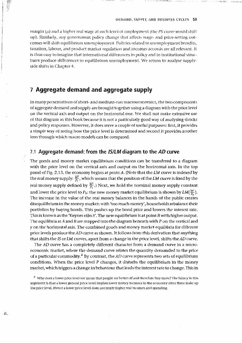
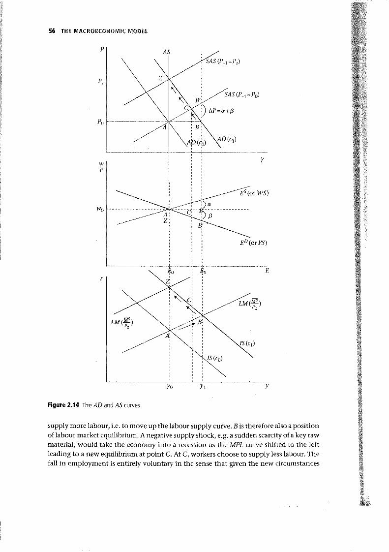