LOCALLY REFINED SPLINES FOR COMPACT …

LOCALLY REFINED SPLINES FOR COMPACT REPRESENTATION AND ANALYSES OF GEOSPATIAL BIG DATATor Dokken, Vibeke Skytt and Oliver BarrowcloughDepartment of Mathematics and Cybernetics SINTEF Digital, Oslo, Norway

Mathematical Models and Methods in Earth and Space Science, Rome Tor Vergata - 19-22 March 2019

Background • SINTEF has addressed research on and industrial uses of polynomial splines

for four decades in cooperation with the University of Oslo

• In the start the focus was Computer Aided Design. Now applications are within Big Data representation and Analysis, Artificial Intelligence, Additive Manufacturing (Representation, design and simulation)

• 2012- 2016 fp7 IP IQmulus targeting big geospatial data (Lidar, sonar,…). • SINTEF focus on compact representation and analysis of sea bottom data

• 2017-2021 IKTPluss ANALYST (Norwegian AI and big data project)• Hydrographic office of the Norwegian Mapping Authorities as partner.

2


Polynomial splines

• A freeform curve (e.g., contour curve in a map) can be represented as a sequence of polynomial segments (degree 1, 2, 3 or higher) where adjacent segments meet with a specified continuity

• A sculptured surface can be represented as a patchwork of bi-variate polynomial patches where adjacent patches meet a specified continuity

• For smooth curves and surfaces piecewise polynomial representation (splines) are much more compact than linear pieces (chains of straight lines or triangulations)

• B-splines are regarded as well suited for the representation of polynomial splines

3


Tensor product B-splines surfaces

• Traditionally B-splines surfaces have been represented using spline spaces that are a tensor product of two univariate spline spaces

• The resulting parameter domain will have a regular grid structure

• Refinement (adding new degrees of freedom) will have effect across the domain

4


Locally refined spline surfaces – add degrees of freedom where needed

5

Surface Polynomial patches, locally refined spline surface

Polynomial patches, tensor-product spline surface version


• At the start of the video we have a bi-variate tensor product B-spline space of bi-degree (2,2)

• Each yellow button represent the vertex (coefficient) of a B-spline. (At the start a regular grid)

• Successive knotline segments are inserted, splitting B-splines and adding new vertices.

• Note: The right continuity over T-joints is coded into the B-splines.

6

LR B-spline refinement

Please click the link below to view the video of K.A. Johannessen, SINTEF Digitalhttps://youtu.be/vFyXs-72qYY


https://youtu.be/vFyXs-72qYY

Starting from tensor product spline space of bi-degree (2,2) – open knots

7


Split one B-spline – increase by one degree of freedom

8


Split from boundary - insert three degrees of freedom

9


Example of B-spline

10


Additional refinements

11


Iterative algorithm for LR B-spline surface approximation

• Input: point cloud, threshold, maximum number of iterations

• Algorithm:• Make a lean approximation on a regular grid

• Compute distances between points and surface approximation

• While (max err > threshold AND number of iterations < max number)

• Refine the surface in regions where the error is above threshold• Compute approximation given the current degrees of freedom

• Output: LR B-spline surface, accuracy information

12


The examples are based on point clouds acquired by single- and multi-beam sonar

• The point clouds consequently have a striped structure

• Multiple point clouds have been registered into the same coordinate system

• We have experienced that making smooth surface approximations of geospatial data highlight features, outliers and registration problems.

13


Examples from IQmulus fp7 IPBritish Channel

• Work performed together with HR Wallingford

• Data courtesy HR Wallingford, SeaZone• 14.6 Million points (280 Mbyte)

• Tolerance 0.5 m

• 6 levels of refinement

• Starting from a tensor product B-spline space that is trimmed to only address the areas that are covered by points.

• Bi-degree (2,2) LR B-spline approximation

14


Initial approximation of 14.6 mill points(280 Mbyte)

15

Number of points 14.6 mill

No. of coefs. 196

Surface file size 26 KB

Max. dist 12.8 m.

Average dist 1.42 m.

# points, dist > 0.5 m 9.9 mill

Polynomial patches in the parameter domain of the surface (bi-quadratic)

Approximating surface

Green points at least 0.5m below surfaceWhite points within 0.5 m of surfaceRed points at least 0.5 m above surface

Data courtesy HR Wallingford, SeaZone

Elevation interval: ~50 m.



No. of coefs. 507


Max. dist 10.5 m.



First iteration

16Polynomial patches in the parameter domain of the surface







No. of coefs. 1336


Max. dist 8.13 m.



Second iteration








No. of coefs. 3563


Max. dist 6.1 m.



Third iteration








No. of coefs. 9273


Max. dist 6.0 m.



Fourth iteration








No. of coefs. 23002

Surface file size 1.6 MB

Max. dist 5.3 m.


# points, dist > 0.5 m 244 850

Fifth iteration








No. of coefs. 23002


Max. dist 5.3 m.


# points, dist > 0.5 m 244 850

Sixth iteration







No. of coefs. 52595


Max. dist 5.4 m.


# points, dist > 0.5 m 75 832


Running through the iterations

28

196 coefficients (9.9 mill outside tol.)

507 coefficients(7.3 mill outside tol.)

1 336 coefficients(3.9 mill outside tol.)



23 002 coefficients(244 850 outside tol.)

52 595 coefficients(75 832 outside tol.)


• Green points at least 0.5m below surface

• White points within 0.5 m of surface

• Red points at least 0.5 m above surface


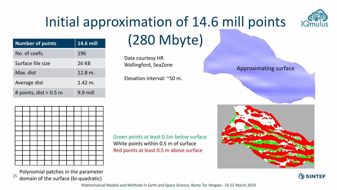
• The Norwegian Hydrographic Service is the authoritative source for nautical publications in Norwegian marine areas, at total of 2.3 million square km.

• Data acquisition rates for bathymetry alone is in the range of multiple petabytes (Pb) per year.29

Small example from a large data set from Søre Sunnmøre, Norway

Images generated using the web-pages of the Norwegian Mapping Authorityhttps://www.kartverket.no/en/


https://www.kartverket.no/en/

Details from pointset with outliers.Idea: Approximate smooth part of point set

30


Example: Extraction of the smooth component

We use a small data set to be able to show visual details

• Data set 641 141 points , file size 26 Mbyte

• LR B-spline approximation on the complete data set: Surface 7.3 Mbyte

Comparing with approximation where non-smooth data points are removed

• Compute rough LR B-spline approximation on the complete data set

• Identify and remove points outside of tolerance, 623 722 points remain

• Calculate the smooth component by using LR B-spline approximation on resulting data set of 25Mbyte giving a LR B-spline surface of 1.7 Mbyte

31


Total data set. In the reduced (smooth) dataset red and green points are removed, white are kept

32

White means higher density of points

Red/green structure related to variable angular accuracy of sonar?


Approximation of whole point set (26 Mbyte) Resulting surface 7.3 Mbyte

Approximation of smooth component (25 Mbyte) Resulting surface 1.7 Mbyte

33

Whole point set vs smooth subset: Surface


Approximation of whole data set

# points approximated 641 141

# coefficients 106 789

⁄# coefficients # points approximated 16,66%

# of elements 122 063

Max distance (Note: Large outlier) 23.7m

Average distance 0.08m

Average distancepoints outside tolerance

0.91m

# Original points outside tolerance 9 350

Surface size 7.3 Mbyte

Approximation of smooth subset

# points approximated 623 722

# coefficients 24 837

⁄# coefficients # points approximated 3.98%

# of elements 28 473

Max distance (Note: No large outlier) 0.80m

Average distance 0.068m

Average distancepoints outside tolerance

0.55m

# Original points outside tolerance 18 002

Surface size 1.7 Mbyte

34

Comparison of surfaces




35

Whole point set vs smooth subset: Surface


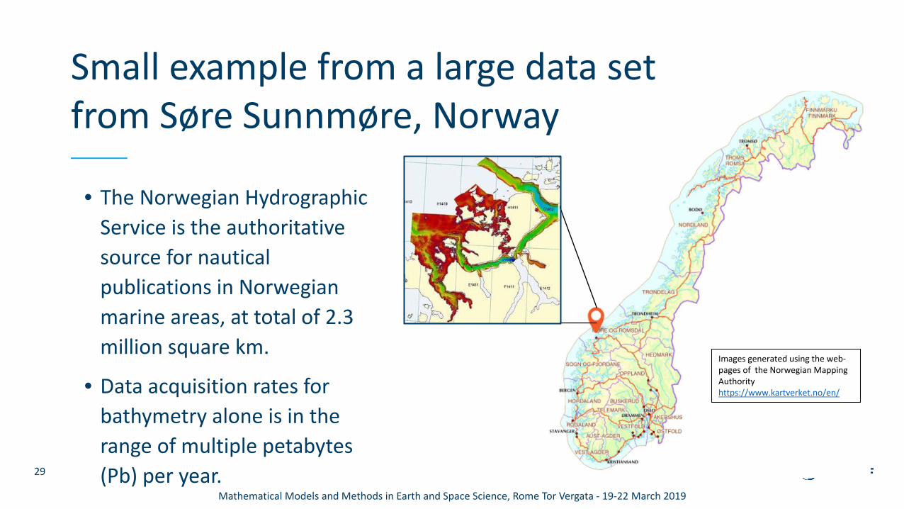
Approximation of whole point set (26 Mbyte) Resulting surface 7.3 Mbyte (122 063 elements)

Approximation of smooth component (25 Mbyte) Resulting surface 1.7 Mbyte (28 473 elements)

36

Whole vs smooth subset: Polynomial pieces


37




38

Points outside toleranceComparison with complete data set

White means higher density of points

Rocky surface not soft. Better to use parametric surface

Red/green structure related to variable angular accuracy of sonar?




39

Whole vs smooth subset: Rocky portion

The many extra degrees of freedom to the left might introduce oscillations giving artificial details.




40

Whole vs smooth subset: Points outside tol.

Alternative handling of points outside tolerance either local triangulation or local parametric surface.


Surface size versus point cloud size• Original data set contains approx. 58 million points• We perform successive thinning of the point cloud and approximate

with fixed parameters: • 0.5 m threshold, 6 iteration levels• Results are very stable showing that the resulting LR B-spline grid is

more dependent on the features of the terrain than the number of points in a scan.

41

Surface size ≈ 3.7 MB

No. points File size No. coefs. Max. error Average error Average outside Prop. OOT points

58 578 420 1.1 GB 53 454 5.55 0.092 0.66 0.56%

29 289 210 559 MB 52 709 5.39 0.092 0.66 0.55 %

14 644 406 280 MB 52 595 5.39 0.093 0.65 0.52 %

7 322 302 140 MB 52 611 5.33 0.093 0.65 0.47 %

3 661 151 70 MB 53 628 5.25 0.093 0.65 0.41%

1 830 575 35 MB 51 124 3.24 0.094 0.65 0.40 %Mathematical Models and Methods in Earth and Space Science, Rome Tor Vergata - 19-22 March 2019

Relevance of LR B-spline approximations for grid structured data

• Each wavelength in a multispectral image can be approximated individually or simultaneously with LR B-splines

• In scattered data there are holes in the data coverage, grid structured data has less holes

• Multi imagery can be put in a common coordinate system and a reference LR B-spline model calculated combining information from the individual images

• Later check for changes can be performed by (fast) evaluation of the LR B-spline model

42


Local spline approximation technologies

• T-splines (2003). Refinement in the B-spline vertex mesh, works well for bi-cubic surfaces.

• Truncated Hierarchical B-splines (THB) (2012). Refinement based on uniform spline spaces defined over dyadic sequence of grids. Works for all degrees and dimensions. Enforces many extra degrees of freedom.

• Locally Refined B-splines (LRB) (2013). Direct refinement of the spline space by insertion of "mesh rectangles". Works for all degrees and dimensions. Allows lean refinements.

LR B-spline the most flexible approach and contains the spline spaces of T-splines and THB.

43


Conclusion

• Approximation of big data by locally refined spline spaces allows compact representation of the smooth component of the data

• The difference between the smooth component and the original dataset highlights the none smooth components. The can represent:• Outliers and noise in the data

• Problems in registration of multiple data sets into the same coordinate system

• Actual none smooth features in the data set

44


Technology for a better society

LOCALLY REFINED SPLINES FOR COMPACT …

Documents

Transcript of LOCALLY REFINED SPLINES FOR COMPACT …