Interpolating Splines
32
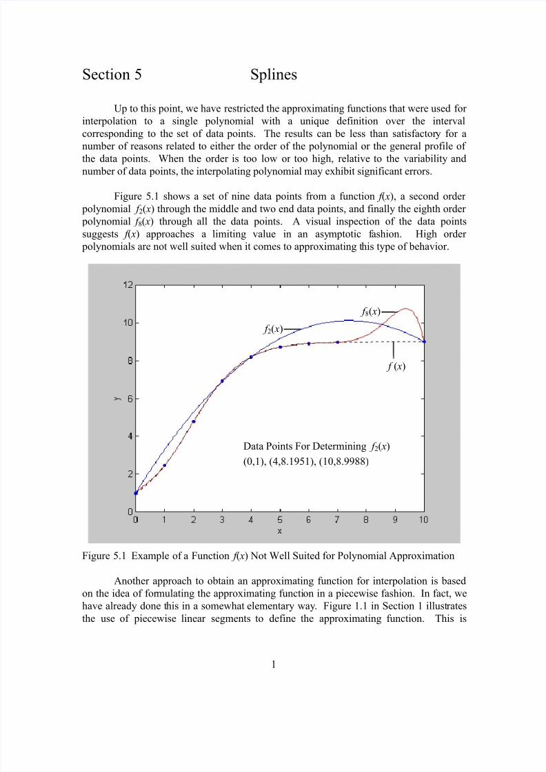
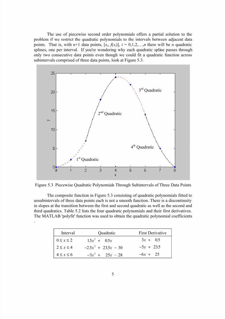
1 Section 5 Splines Up to this point, we have restricted the approximating functions that were used for interpolation to a single polynomial with a unique definition over the interval corresponding to the set of data points. The results can be less than satisfactor y for a number of reasons related to either the order of the polynomial or the general profile of the data points. When the order is too low or too high, relative to the variability and number of data points, the interpolating polynomial may exhibit significant errors. Figure 5.1 shows a set of nine data points from a function f ( x), a second order polynomial f 2 ( x) through the middle and two end data points, and finally the eighth order polynomial f 8 ( x) through all the data points. A visual inspection of the data points suggests f ( x) approaches a limiting value in an asy mptotic f ashion. High order polynomials are not well suited when it comes to approximating t his type of behavior. Figure 5.1 Example of a Function f ( x) Not Well Suited for Polynomial Approximation Another approach to obtain an approximating function for interpolation is based on the idea of for mulating the approximating functi on in a piecewise fashion. In fact, we have already done t his in a somewhat elementary way. Figure 1.1 in Section 1 illust rates the use of piecewise linear segments to define the approximating function. This is f 2 ( x) f ( x) Data Points For Determining f 2 ( x) (0,1), (4,8.1951), (10,8.9988) f 8 ( x)
-
Upload
mykingboody2156 -
Category
Documents
-
view
250 -
download
0
Transcript of Interpolating Splines
8/13/2019 Interpolating Splines
http://slidepdf.com/reader/full/interpolating-splines 1/32
1
Section 5 Splines
Up to this point, we have restricted the approximating functions that were used for
interpolation to a single polynomial with a unique definition over the interval
corresponding to the set of data points. The results can be less than satisfactory for anumber of reasons related to either the order of the polynomial or the general profile of
the data points. When the order is too low or too high, relative to the variability and
number of data points, the interpolating polynomial may exhibit significant errors.
Figure 5.1 shows a set of nine data points from a function f ( x), a second order
polynomial f 2( x) through the middle and two end data points, and finally the eighth order
polynomial f 8( x) through all the data points. A visual inspection of the data points
suggests f ( x) approaches a limiting value in an asymptotic fashion. High order
polynomials are not well suited when it comes to approximating this type of behavior.
Figure 5.1 Example of a Function f ( x) Not Well Suited for Polynomial Approximation
Another approach to obtain an approximating function for interpolation is based
on the idea of formulating the approximating function in a piecewise fashion. In fact, we
have already done this in a somewhat elementary way. Figure 1.1 in Section 1 illustrates
the use of piecewise linear segments to define the approximating function. This is
f 2( x)
f ( x)
Data Points For Determining f 2( x)
(0,1), (4,8.1951), (10,8.9988)
f 8( x)
8/13/2019 Interpolating Splines
http://slidepdf.com/reader/full/interpolating-splines 2/32
2
equivalent to using multiple first order interpolating polynomials restricted to intervals
between adjacent data points.
Suppose we wish to approximate a function f ( x), defined in tabular form by a set
of data points [ xi, f ( xi)], i = 0,1,2,…,n with lower order polynomials, each valid for a
limited portion of the interval x0 ≤ x ≤ xn. These lower order polynomials are referred toas spline functions. The term originates from drafting where a smooth curve is drawn
through a set of control points using a flexible strip called a "spline". The spline is
weighted at various points along its length to keep it in contact with the drafting surface
as the curve is drawn. The simplest implementation is to use linear splines in the
intervals between consecutive data points. Doing this, we denote the approximating
function F 1( x) and the "n" linear splines which comprise it as f 1,i( x). This leads to
F x
f x x x x
f x x x x
f x x x x
i i i
n n n
1
1 1 0 1
1 1
1 1
( )
( ),
( ),
( ),
,
,
,
=
≤ ≤
≤ ≤
≤ ≤
R
S
||
|||
T
|||||
−
−
(5.1)
Using Newton first order divided-difference interpolating polynomials for the
linear splines,
F x
a b x x x x x
a b x x x x x
a b x x x x x
i i i i i
n n n n n
1
1 1 0 0 1
1 1
1 1
( )
( ),
( ),
( ),
=
+ − ≤ ≤
+ − ≤ ≤
+ − ≤ ≤
R
S
|||||
T
|||||
− −
− −
(5.2)
The coefficients ai and bi define the individual splines f xi1, ( ) and are given by
a f x i ni i= =−( ), , , ,...,1 1 2 3 (5.3)
b f x f x
x xi ni
i i
i i
= −
−=−
−
( ) ( ), , , ,...1
1
1 2 3 (5.3a)
8/13/2019 Interpolating Splines
http://slidepdf.com/reader/full/interpolating-splines 3/32
8/13/2019 Interpolating Splines
http://slidepdf.com/reader/full/interpolating-splines 4/32
4
»xint=0.5:1:9.5»Fint=interp1(x,F_x,xint)
xint = 0.5000 1.5000 2.5000 3.5000 4.5000 5.5000 6.5000 7.5000 8.5000 9.5000
Fint = 1.7285 3.6140 5.8602 7.5723 8.4551 8.8091 8.9353 8.9727 8.9831 8.9936
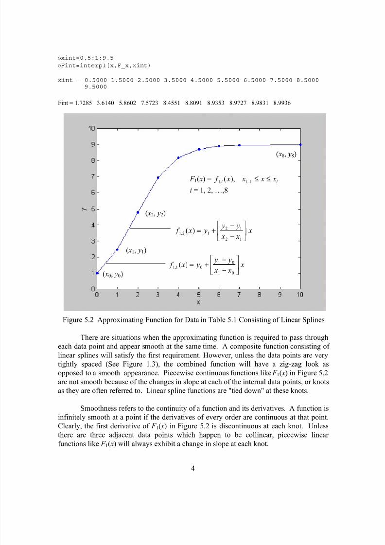
Figure 5.2 Approximating Function for Data in Table 5.1 Consisting of Linear Splines
There are situations when the approximating function is required to pass through
each data point and appear smooth at the same time. A composite function consisting of
linear splines will satisfy the first requirement. However, unless the data points are very
tightly spaced (See Figure 1.3), the combined function will have a zig-zag look as
opposed to a smooth appearance. Piecewise continuous functions like F 1( x) in Figure 5.2
are not smooth because of the changes in slope at each of the internal data points, or knotsas they are often referred to. Linear spline functions are "tied down" at these knots.
Smoothness refers to the continuity of a function and its derivatives. A function is
infinitely smooth at a point if the derivatives of every order are continuous at that point.
Clearly, the first derivative of F 1( x) in Figure 5.2 is discontinuous at each knot. Unless
there are three adjacent data points which happen to be collinear, piecewise linear
functions like F 1( x) will always exhibit a change in slope at each knot.
( x0, y0)
( x1, y1)
( x2, y2)
( x8, y8)
f x y y y
x x x1 2 1
2 1
2 1
, ( ) = + −
−
L
NM
O
QP
f x y y y
x x x1 1 0
1 0
1 0
, ( ) = + −
−
L
NM
O
QP
F 1( x) = f x x x xi i i1 1, ( ), − ≤ ≤
i = 1, 2, …,8
8/13/2019 Interpolating Splines
http://slidepdf.com/reader/full/interpolating-splines 5/32
8/13/2019 Interpolating Splines
http://slidepdf.com/reader/full/interpolating-splines 6/32
6
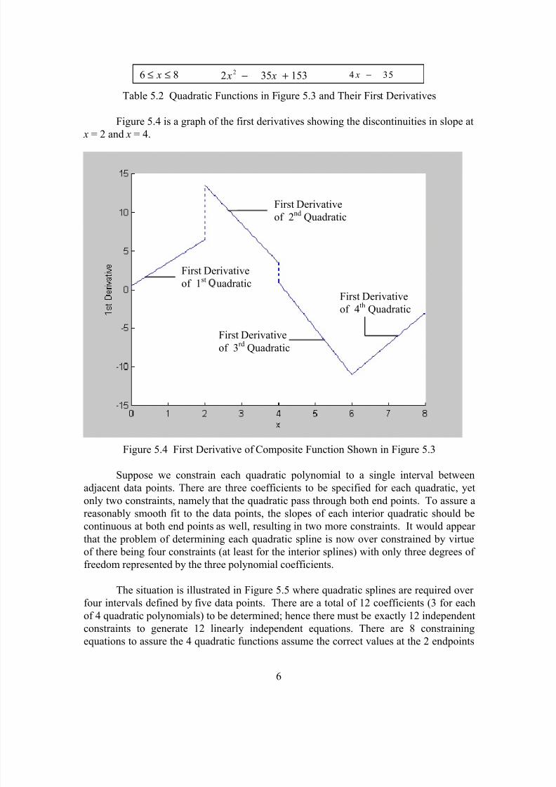
6 8≤ ≤ x 2 35 1532 x x− + 4 35 x −
Table 5.2 Quadratic Functions in Figure 5.3 and Their First Derivatives
Figure 5.4 is a graph of the first derivatives showing the discontinuities in slope at
x = 2 and x = 4.
Figure 5.4 First Derivative of Composite Function Shown in Figure 5.3
Suppose we constrain each quadratic polynomial to a single interval between
adjacent data points. There are three coefficients to be specified for each quadratic, yet
only two constraints, namely that the quadratic pass through both end points. To assure a
reasonably smooth fit to the data points, the slopes of each interior quadratic should be
continuous at both end points as well, resulting in two more constraints. It would appear
that the problem of determining each quadratic spline is now over constrained by virtue
of there being four constraints (at least for the interior splines) with only three degrees of freedom represented by the three polynomial coefficients.
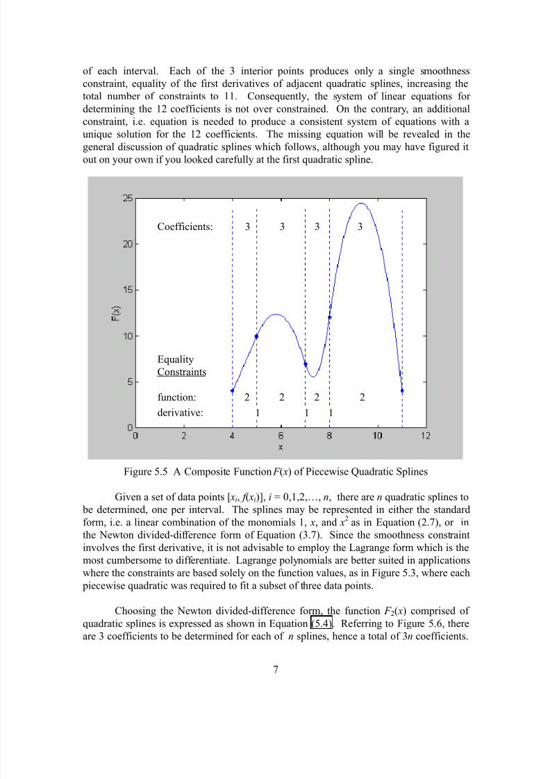
The situation is illustrated in Figure 5.5 where quadratic splines are required over
four intervals defined by five data points. There are a total of 12 coefficients (3 for each
of 4 quadratic polynomials) to be determined; hence there must be exactly 12 independent
constraints to generate 12 linearly independent equations. There are 8 constraining
equations to assure the 4 quadratic functions assume the correct values at the 2 endpoints
First Derivativeof 1st uadratic
First Derivative
of 2nd Quadratic
First Derivative
of 3rd Quadratic
First Derivative
of 4th Quadratic
8/13/2019 Interpolating Splines
http://slidepdf.com/reader/full/interpolating-splines 7/32
7
of each interval. Each of the 3 interior points produces only a single smoothness
constraint, equality of the first derivatives of adjacent quadratic splines, increasing the
total number of constraints to 11. Consequently, the system of linear equations for
determining the 12 coefficients is not over constrained. On the contrary, an additional
constraint, i.e. equation is needed to produce a consistent system of equations with a
unique solution for the 12 coefficients. The missing equation will be revealed in thegeneral discussion of quadratic splines which follows, although you may have figured it
out on your own if you looked carefully at the first quadratic spline.
Figure 5.5 A Composite Function F ( x) of Piecewise Quadratic Splines
Given a set of data points [ xi, f ( xi)], i = 0,1,2,…, n, there are n quadratic splines to
be determined, one per interval. The splines may be represented in either the standard
form, i.e. a linear combination of the monomials 1, x, and x2 as in Equation (2.7), or in
the Newton divided-difference form of Equation (3.7). Since the smoothness constraint
involves the first derivative, it is not advisable to employ the Lagrange form which is themost cumbersome to differentiate. Lagrange polynomials are better suited in applications
where the constraints are based solely on the function values, as in Figure 5.3, where each
piecewise quadratic was required to fit a subset of three data points.
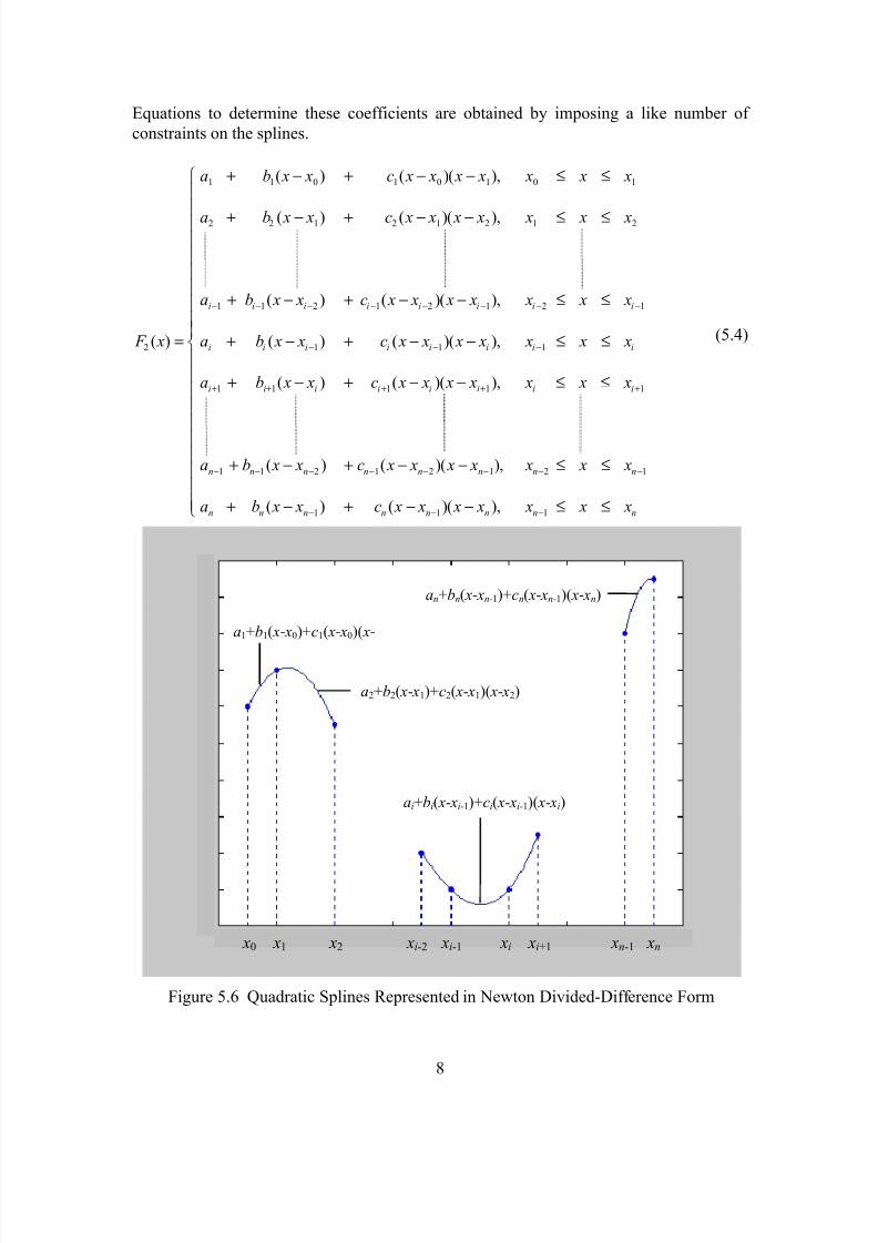
Choosing the Newton divided-difference form, the function F 2( x) comprised of
quadratic splines is expressed as shown in Equation (5.4). Referring to Figure 5.6, there
are 3 coefficients to be determined for each of n splines, hence a total of 3n coefficients.
Coefficients: 3 3 3 3
Equality
Constraints
function: 2 2 2 2
derivative: 1 1 1
8/13/2019 Interpolating Splines
http://slidepdf.com/reader/full/interpolating-splines 8/32
8
Equations to determine these coefficients are obtained by imposing a like number of
constraints on the splines.
F x
a b x x c x x x x x x x
a b x x c x x x x x x x
a b x x c x x x x x x x
a b x x c x x x x x x x
a b x x c x x
i i i i i i i i
i i i i i i i i
i i i i i
2
1 1 0 1 0 1 0 1
2 2 1 2 1 2 1 2
1 1 2 1 2 1 2 1
1 1 1
1 1 1
( )
( ) ( )( ),
( ) ( )( ),
( ) ( )( ),
( ) ( )( ),
( ) (
=
+ − + − − ≤ ≤
+ − + − − ≤ ≤
+ − + − − ≤ ≤
+ − + − − ≤ ≤
+ − + −
− − − − − − − −
− − −
+ + + )( ),
( ) ( )( ),
( ) ( )( ),
x x x x x
a b x x c x x x x x x x
a b x x c x x x x x x x
i i i
n n n n n n n n
n n n n n n n n
− ≤ ≤
+ − + − − ≤ ≤
+ − + − − ≤ ≤
R
S
|
|||||||||
T
||||||||||
+ +
− − − − − − − −
− − −
1 1
1 1 2 1 2 1 2 1
1 1 1
(5.4)
Figure 5.6 Quadratic Splines Represented in Newton Divided-Difference Form
a1+b1( x- x0)+c1( x- x0)( x-
a2+b2( x- x1)+c2( x- x1)( x- x2)
an+bn( x- xn-1)+cn( x- xn-1)( x- xn)
ai+bi( x- xi-1)+ci( x- xi-1)( x- xi)
x0 x1 x2 xi-2 xi-1 xi xi+1 xn-1 xn
8/13/2019 Interpolating Splines
http://slidepdf.com/reader/full/interpolating-splines 9/32
9
The first set of equations constrain the quadratic splines to the data point function
values at the end points of their respective intervals. This assures F 2( x) will be a
piecewise continuous function through the entire set of data points.
I. Interval End Point Function Values Must Equal Data Point Values:
F 2( xi) = f ( xi), i = 0, 1, 2, …, n (5.5)
For the first interval,
F x a b x x c x x x x2 0 1 1 0 0 1 0 0 0 1( ) ( ) ( )( )= + − + − − (5.6)
f x a( )0 1= (5.7)
F x a b x x c x x x x2 1 1 1 1 0 1 1 0 1 1( ) ( ) ( )( )= + − + − − (5.8)
f x f x b x x( ) ( ) ( )1 0 1 1 0= + − (5.9)
b f x f x
x x1
1 0
1 0
= −
−
( ) ( )(5.10)
Evaluating the second quadratic spline at the end points of its interval gives
F x a b x x c x x x x2 1 2 2 1 1 2 1 1 1 2( ) ( ) ( )( )= + − + − − (5.11)
f x a( )1 2= (5.12)
F x a b x x c x x x x2 2 2 2 2 1 2 2 1 2 2( ) ( ) ( )( )= + − + − − (5.13)
f x f x b x x( ) ( ) ( )2 1 2 2 1= + − (5.14)
b f x f x
x x2
2 1
2 1
= −
−
( ) ( )(5.15)
Similar constraints apply to the remaining splines. The general form of the
equations are given below.
F x a b x x c x x x xi i i i i i i i i i2 1 1 1 1 1 1( ) ( ) ( )( )− − − − − −= + − + − − (5.16)
a f x i ni i= =−( ), , , ,...,1 1 2 3 (5.17)
F x a b x x c x x x xi i i i i i i i i i2 1 1( ) ( ) ( )( )= + − + − −− − (5.18)
8/13/2019 Interpolating Splines
http://slidepdf.com/reader/full/interpolating-splines 10/32
8/13/2019 Interpolating Splines
http://slidepdf.com/reader/full/interpolating-splines 11/32
11
Example 5.2
A highway engineer must design a new road which will connect two existing
roads. In order to maintain safe clearances from a lake and several structures,measurements were taken to determine several points along the centerline of the proposed
road. The geographical locations of these points, relative to some point of reference, are
given in Table 5.3. Quadratic splines are to be used to specify the equations of the
centerlines for each road segment.
i xi (miles) yi (miles)
0 0.0 1.0
1 0.2 1.0
2 0.6 1.2
3 1.0 1.1
4 1.4 0.6
5 1.6 0.5
6 1.8 0.5
7 2.0 0.5
Table 5.3 End Point Data for Segments of Proposed Roadway
The following MATLAB m-file was written to plot the given centerline points,
determine the quadratic splines, and plot the continuous centerline comprised of the those
splines. The results are illustrated in Figure 5.7 which shows the smooth centerline
trajectory of the proposed connector between the existing roads. (Despite the smooth
appearance of the connecting road, the curvature at certain points may not conform to
existing civil engineering standards for roadway design.)
% Example 5.3x=[0 0.2 0.6 1 1.4 1.6 1.8 2]; % Centerliney=[1 1 1.2 1.1 0.6 0.5 0.5 0.5]; % Data Pointsv=[0 2 0 1.6];plot(x,y,'.') % Plot Centerline Data Pointsxlabel('x (miles)')
ylabel('y (miles')axis(v)hold onaxis manualn=8;% Find Newton Polynomial Coefficientsfor i=1:n-1 a(i)=y(i); b(i)=(y(i+1)-y(i))/(x(i+1)-x(i));end
8/13/2019 Interpolating Splines
http://slidepdf.com/reader/full/interpolating-splines 12/32
12
c(1)=0;for i=2:n-1 factor1=(x(i)-x(i-1))/(x(i)-x(i+1)); factor2=(b(i-1)-b(i))/(x(i)-x(i+1)); c(i)=factor1*c(i-1)+factor2;end % Plot Quadratic Splines
for i=1:n-1 xi=linspace(x(i),x(i+1),100); f2=a(i)+b(i)*(xi-x(i))+c(i)*(xi-x(i)).*(xi-x(i+1)); plot(xi,f2,'-')end
Figure 5.7 Roadway Centerline Consisting of Quadratic Splines
When the data points are equally spaced, i.e.
x x i ni i+ − = = −1 0 1 2 1∆, , , ,..., (5.27)
Equations (5.20) and (5.26) simplify to
b f x f x
i nii i=
−=−( ) ( )
, , ,...,1 1 2 3∆
(5.28)
c c f x f x f x i ni i i i i+ + −= − + − + = −1 2 1 1
12 1 2 3 1
∆( ) ( ) ( ) , , , ,..., (5.29)
Lake
Newton
Lake
Isaac
Mall
Apartments
ExistingRoad
Existing
Road
8/13/2019 Interpolating Splines
http://slidepdf.com/reader/full/interpolating-splines 13/32
13
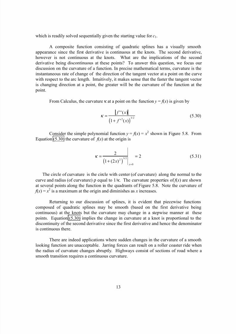
which is readily solved sequentially given the starting value for c1.
A composite function consisting of quadratic splines has a visually smooth
appearance since the first derivative is continuous at the knots. The second derivative,
however is not continuous at the knots. What are the implications of the secondderivative being discontinuous at these points? To answer this question, we focus our
discussion on the curvature of a function. In precise mathematical terms, curvature is the
instantaneous rate of change of the direction of the tangent vector at a point on the curve
with respect to the arc length. Intuitively, it makes sense that the faster the tangent vector
is changing direction at a point, the greater will be the curvature of the function at the
point.
From Calculus, the curvature κ at a point on the function y = f ( x) is given by
κ = +
f x
f x
' ' ( )
' ( )/
1 2 3 2
c h (5.30)
Consider the simple polynomial function y = f ( x) = x2 shown in Figure 5.8. From
Equation (5.30) the curvature of f ( x) at the origin is
κ =+
=
=
2
1 22
23 2
0( )
/
x x
c h(5.31)
The circle of curvature is the circle with center (of curvature) along the normal to thecurve and radius (of curvature) ρ equal to 1/κ . The curvature properties of f ( x) are shown
at several points along the function in the quadrants of Figure 5.8. Note the curvature of
f ( x) = x2 is a maximum at the origin and diminishes as x increases.
Returning to our discussion of splines, it is evident that piecewise functions
composed of quadratic splines may be smooth (based on the first derivative being
continuous) at the knots but the curvature may change in a stepwise manner at these
points. Equation (5.30) implies the change in curvature at a knot is proportional to the
discontinuity of the second derivative since the first derivative and hence the denominator
is continuous there.
There are indeed applications where sudden changes in the curvature of a smooth
looking function are unacceptable. Jarring forces can result on a roller coaster ride when
the radius of curvature changes abruptly. Highways consist of sections of road where a
smooth transition requires a continuous curvature.
8/13/2019 Interpolating Splines
http://slidepdf.com/reader/full/interpolating-splines 14/32
14
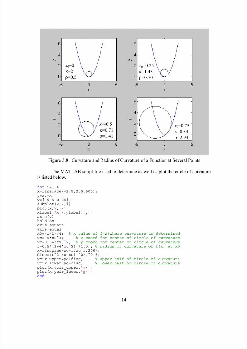
Figure 5.8 Curvature and Radius of Curvature of a Function at Several Points
The MATLAB script file used to determine as well as plot the circle of curvature
is listed below.
for i=1:4x=linspace(-2.5,2.5,500);y=x.*x;v=[-5 5 0 10];subplot(2,2,i)plot(x,y,'-')xlabel('x'),ylabel('y')axis(v)hold onaxis squareaxis equalx0=(i-1)/4; % x value of f(x)where curvature is determinedxc=-4*x0^3; % x coord for center of circle of curvatureyc=0.5+3*x0^2; % y coord for center of circle of curvaturer=0.5*(1+4*x0^2)^(1.5); % radius of curvature of f(x) at x0x=linspace(xc-r,xc+r,200);disc=(r^2-(x-xc).^2).^0.5;ycir_upper=yc+disc; % upper half of circle of curvatureycir_lower=yc-disc; % lower half of circle of curvatureplot(x,ycir_upper,'g-')plot(x,ycir_lower,'g-')end
x0=0
κ =2
ρ=0.5
x0=0.25
κ =1.43
ρ=0.70
x0=0.5
κ =0.71
ρ=1.41
x0=0.75
κ =0.34
ρ=2.93
8/13/2019 Interpolating Splines
http://slidepdf.com/reader/full/interpolating-splines 15/32
8/13/2019 Interpolating Splines
http://slidepdf.com/reader/full/interpolating-splines 16/32
16
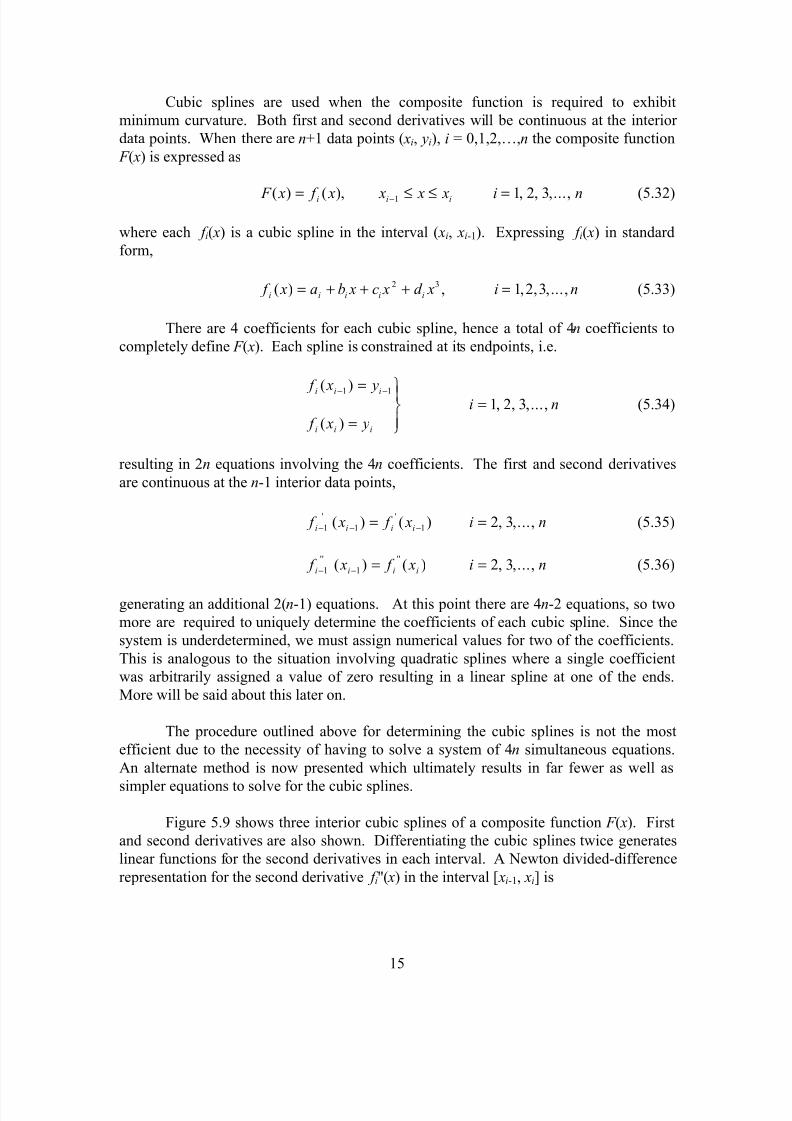
f x A x x A A
x xi i i
i i
i i
' ' ( ) ( )= + − −
−− −
−
−
1 11
1
(5.37)
where Ai-1 and Ai are the numerical values, yet to be determined, of the second derivative
at xi-1 and xi respectively, (See Figure 5.9).
Figure 5.9 Cubic Splines and Their First Two Derivatives
Integrating the second derivative in Equation (5.37) twice, yields expressions for
f i'( x) and f i( x) with constants of integration present.
f x A A
x x
x x A x xi
i i
i i
i
i i i' ( ) ( )= −
−
F H G
I K J
−+ − +−
−
−
− −1
1
1
2
1 12
b gα (5.38)
f x A A
x x
x x A
x x x xi
i i
i i
i
i
i
i i i( ) ( )= −
−
F H G
I K J
−+
−+ − +−
−
−
−
−
−1
1
1
3
1
1
2
16 2
b g b gα β (5.39)
The constants of integration are determined from the endpoint constraints of
Equation (5.34). The result is
xi-2 xi-1 xi xi+1
xi-2 xi-1 xi xi+1
i-2 xi-1 xi xi+1
F "( x)
F '( x)
F ( x)
Ai-2
Ai-1
Ai
yi-2
yi-1
yi
f i( x)
f i-1( x)
8/13/2019 Interpolating Splines
http://slidepdf.com/reader/full/interpolating-splines 17/32
17
β i i y i n= =−1 1 2 3, , , ,..., (5.40)
α ii i
i i
i ii i
y y
x x
A A x x i n=
−
−−
+F H G
I K J
− =−
−
−−
1
1
11
2
61 2 3b g, , , ,..., (5.41)
Substituting Equations (5.40) and (5.41) into Equation (5.39) yields expressions
for the cubic splines which pass through the data points ( xi, yi), i = 0,1,2,…, n.
f x A A
x x x x
A x xi
i i
i i
ii
i( ) ( ) ( )= −
−
L
NM
O
QP − + −−
−
−−
−1
1
1
3 11
2
6 2b g(5.42)
+ −
−−
+F H G
I K J
−L
NM
O
QP − + =−
−
−− − −
y y
x x
A A x x x x y i ni i
i i
i i
i i i i
1
1
11 1 1
2
61 2 3b g ( ) , , , ,...,
At first glance it appears that we may have complicated things unnecessarily due
to the presence of the second derivative terms Ai and Ai-1 in Equation (5.42). On the
positive side, however, we are not confronted with a system of 4n simultaneous equations
as would be the case if we employed the standard polynomial form to represent the cubic
splines. In fact, all that remains is a way of determining the constants Ai, i = 0, 1, 2, …, n.
Equations for these constants are obtained by imposing the continuity requirement
of the first derivative at the knots, Equation (5.35). Note, continuity of the second
derivative at each knot is assured by virtue of Equation (5.37). The process is
straightforward but tedious due to the manipulation of numerous terms appearing in the
expressions for the first derivatives ′− − f xi i1 1( ) and ′ − f xi i( )1 . After much simplification,the result is
x x A
x x A
x x A
y y
x x
y y
x x
i ii
i ii
i i
ii i
i i
i i
i i
−F H G
I K J
+ −F
H G I
K J +
−F H G
I K J
= −
−−
−
−− −
−− −
−−
−
− −
− −
1 21
1 2
21
1
1 2
1 26 3 6(5.43)
Equation (5.43) applies for i = 2,3,…,n which accounts for n-1 equations relating
the n+1 constants Ai, i = 0,1,2,…,n. It is customary to select or compute numerical
values for A0 and An based on additional information or requirements imposed on the
endmost splines. For example, choosing A0 = An = 0, produces what is referred to as a
"natural" cubic spline. In this case, the spline is relaxed at both ends approaching straight
lines at the endpoints. A "clamped" cubic spline results when the endpoint constants A0
and An are calculated based on known values for the first derivatives at the endpoints, i.e.
′ f x1 0( ) and ′ f xn n( ). Alternatively, A0 and An can be extrapolated values based on A1, A2
and An-2, An-1 respectively. Finally, selecting A0 = A1 and An = An-1 forces the two end
splines to reduce to quadratics (see Equation (5.37)).
8/13/2019 Interpolating Splines
http://slidepdf.com/reader/full/interpolating-splines 18/32
18
Composite functions made up of cubic splines are reasonably smooth in
appearance because the curvature of the individual splines connecting the data points is
moderate in comparison to that of a single high order polynomial defined over the entire
range of data points. Recall from Equation (5.30) that the curvature of a function is
directly related to the second derivative. Clearly, large second derivatives imply the first
derivative is changing rapidly and therefore the slope of the tangent vector is doinglikewise, resulting in significant curvature. In other words, given the choice of two
interpolating functions, the one with the smaller (in some average sense) second
derivative is preferable. It can be shown that of all possible interpolating functions which
are twice differentiable, the natural cubic spline has the least curvature in the mean square
sense. In mathematical terms, the integral g x dx x
xn
( )2
0
z is a minimum when the integrand
g ( x) is a natural cubic spline.
Example 5.3
In Example 5.2, a company is planning on bidding for the contract to build the
proposed road. In order to estimate the cost, it must know the length of road to be
constructed. Cubic splines are to be used to describe the road geometry and calculate its
length.
An m-file was written to produce a natural spline fit through the data points from
Table 5.3. From Equation (5.43), a 6 6× coefficient matrix X and 6 1× constant vector
b are created. The 6 1× vector a of second derivatives is the solution to the system of
equationsXa b= where
= = =
1
2
3
4
5
6
X b a
15
115
115
415
115
115
415
115
115
15
130
130
215
130
115
215
12
34
34
12
0 0 0 0
0 0 0
0 0 0
0 0 0
0 0 0
0 0 0 0
1
0
L
N
MMMMMMMM
O
Q
PPPPPPPP
−
−
L
N
MMMMMMMM
O
Q
PPPPPPPP
L
N
MMMMMMM
O
Q
PPPPPPP
A
A
A
A
A
A
The cubic splines are then determined from Equation (5.42) and plotted in Figure
5.10 along with the data points. For comparison, the road using quadratic splines
determined in Example 5.2 and plotted in Figure 5.7 is redrawn. The m-file listingfollows.
% Example 5.3 and Figure 5.10% A natural cubic spline is fit to the data points defined% by vectors x and y. A0 and An in Equation (5.43)are both zero.x=[0 0.2 0.6 1 1.4 1.6 1.8 2];y=[1 1 1.2 1.1 0.6 0.5 0.5 0.5];v=[0 2 0 1.6];
8/13/2019 Interpolating Splines
http://slidepdf.com/reader/full/interpolating-splines 19/32
19
plot(x,y,'.')axis(v)axis manualhold onn=7; % Number of data pointsX=zeros(n-1,n-1); % X is (n-1) by (n-1)%Create first row of X matrix and b vector
X(1,1)=(x(3)-x(1))/3;X(1,2)=(x(3)-x(2))/6;b(1)=(y(3)-y(2))/(x(3)-x(2)) - (y(2)-y(1))/(x(2)-x(1));% Create rows 2 thru n-2 of X matrix and b vector for i=2:n-2 X(i,i-1)=(x(i+1)-x(i))/6; X(i,i)=(x(i+2)-x(i))/3; X(i,i+1)=(x(i+2)-x(i+1))/6; b(i)=(y(i+2)-y(i+1))/(x(i+2)-x(i+1)) - (y(i+1)-y(i))/(x(i+1)-x(i)); end% Create (n-1)st row of X matrix and b vectorX(n-1,n-2)=(x(n)-x(n-2))/6;X(n-1,n-1)=(x(n+1)-x(n-1))/3;b(n-1)=(y(n+1)-y(n))/(x(n+1)-x(n)) - (y(n)-y(n-1))/(x(n)-x(n-1));a=inv(X)*b'; % Find a=[A(1)....A(n-1)]for i=1:n dx=x(i+1)-x(i); dy=y(i+1)-y(i); xspace=linspace(x(i),x(i+1),75); xx=xspace-x(i); if (i==1) T1=(1/6)*(a(1)/dx)*xx.^3; T3=((dy/dx)-(a(1)/6)*dx)*xx + y(1); f_1=T1+T3; plot(xspace,f_1,'-') % Plot 1st cubic spline elseif(i~=1&i~=n) T1=(1/6)*((a(i)-a(i-1))/dx)*xx.^3; T2=(a(i-1)/2)*xx.^2; T3=((dy/dx)-((a(i)+2*a(i-1))/6)*dx)*xx + y(i);
f_i=T1+T2+T3; plot(xspace,f_i,'-') % Plot 2nd thru (n-1)st cubic spline elseif(i==n) T1=(1/6)*(-a(n-1)/dx)*xx.^3; T2=(a(i-1)/2)*xx.^2; T3=((dy/dx)-(a(n-1)/3)*dx)*xx + y(n); f_n=T1+T2+T3; plot(xspace,f_n,'-') % Plot nth cubic spline endend
As you might expect MATLAB has its own built-in routine for cubic splines. The
statement yi = spline(x, y, xi) invokes the cubic spline function where arrays x and y
define the data points while (xi, yi) are the smoothed point(s) in between them. Instead of a natural spline, MATLAB constrains the third derivatives of the first two and last two
cubic splines to be equal. The constants A0 and An are not zero; however the vector a =
[ A0 A1…. An]T is uniquely determined. The 'spline' function exploits the sparse nature of
the coefficient matrix obtained from Equation (5.43) and is therefore more efficient than
matrix inversion to solve the equations.
8/13/2019 Interpolating Splines
http://slidepdf.com/reader/full/interpolating-splines 20/32
20
Figure 5.10 Roadway Centerline Determined From Quadratic and Cubic Splines
If you're curious about the coefficients for each cubic spline, you can call 'spline'
with arguments x and y only and it returns a 'pp' or piecewise polynomial array form
which can be decomposed using 'unmkpp' to reveal the polynomial coefficients and other useful information. To illustrate, suppose we use the data points from Example 5.3.
»x=[0 0.2 0.6 1 1.4 1.6 1.8 2];»y=[1 1 1.2 1.1 0.6 0.5 0.5 0.5];pp=spline(x,y);[x_values,spline_coefs,num_splines,num_coefs]=unmkpp(pp)
The following output results.
x _values = 0 0.2000 0.6000 1.0000 1.4000 1.6000 1.8000 2.0000
spline_coefs = -2.0032 2.4359 -0.4070 1.0000 -2.0032 1.2340 0.3269 1.0000 -0.8416 -1.1698 0.3526 1.2000 3.8069 -2.1797 -0.9872 1.1000 -1.8512 2.3886 -0.9037 0.6000 -2.1298 1.2779 -0.1704 0.5000
-2.1298 0.0000 0.0852 0.5000
num_splines = 7
Quadratic Splines
(Example 5.2)
Cubic Splines
(Example 5.3)
8/13/2019 Interpolating Splines
http://slidepdf.com/reader/full/interpolating-splines 21/32
21
num_coefs = 4
Note, the 'pp' array can be used multiple times for interpolation using 'ppval'
without having to recompute the cubic spline coefficients, in the same way the array
resulting from a 'polyfit' call can be used repeatedly with 'polyval'. For example, if we
need the second cubic spline evaluated at 10 equally spaced points or the compositefunction evaluated at 20 equally spaced points, we could write
»yi=ppval(pp,linspace(0.2,0.6,10))»yi=ppval(pp,linspace(0,2,20))
yi=1.0000 1.0168 1.0374 1.0608 1.0859 1.1116 1.1369 1.1608 1.1822 1.2000
yi=1.0000 0.9818 1.0036 1.0513 1.1109 1.1685 1.2099 1.2242 1.2048 1.1460 1.0426 0.9048 0.7586 0.6308 0.5456 0.5042 0.4934 0.4991 0.5063 0.5000
We have yet to calculate the road length as required in Example 5.3. Since 'pp'
describes the entire composite function of cubic splines, its ideal for computing the length
of any section or the entire length of the roadway. A simple procedure for estimating alength of section from x = a to x = b is now presented.
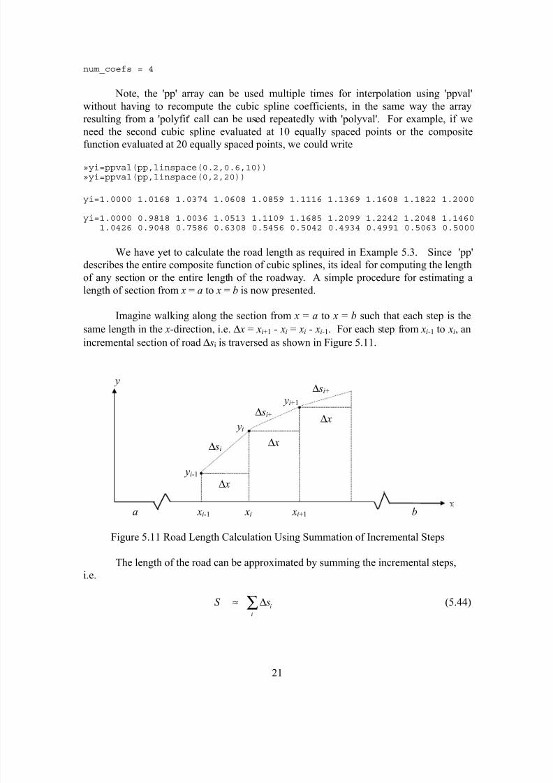
Imagine walking along the section from x = a to x = b such that each step is the
same length in the x-direction, i.e. ∆ x = xi+1 - xi = xi - xi-1. For each step from xi-1 to xi, an
incremental section of road ∆ si is traversed as shown in Figure 5.11.
Figure 5.11 Road Length Calculation Using Summation of Incremental Steps
The length of the road can be approximated by summing the incremental steps,
i.e.
S si
i
≈ ∑ ∆ (5.44)
a xi-1 xi xi+1 b
∆ x
∆ x
∆ x
∆ si
∆ si+
∆ si+
yi
yi+1
yi-1
y
8/13/2019 Interpolating Splines
http://slidepdf.com/reader/full/interpolating-splines 22/32
22
S x yi
i
≈ +∑ ∆ ∆b g b g2 2
12
(5.45)
Note how the 'pp' array is used with the function 'ppval' in the following m-file
listing to find the y coordinates of each step. Since a = 0 and b = 2 correspond to theendpoints, the value for "length" represents the length of the entire road. Also note, the
file was executed twice with different values of "n" to ensure the accuracy of the answer.
%Road Length Calculationx=[0 0.2 0.6 1 1.4 1.6 1.8 2];y=[1 1 1.2 1.1 0.6 0.5 0.5 0.5];pp=spline(x,y);a=0;b=2;n=1000 % Number of points. There are n-1 steps.xi=linspace(a,b,n);dx=xi(2)-xi(1);yi=ppval(pp,xi);
s=0;for i=1:n-1 dyi=yi(i+1)-yi(i); dsi=(dx*dx + dyi.*dyi).^0.5; s=s+dsi;endlength=s
n = 100length = 2.3597
n = 1000length = 2.3599
You probably recognize Equation (5.45) as a step along the way to obtaining anintegral expression. Further discussion of integration and approximation methods is
deferred until the chapter on Numerical Integration.
The next example illustrates the use of splines and low order interpolating
polynomials as a way of representing the thermodynamic properties of a substance.
Example 5.4
The refrigerant in refrigeration system circulates in a closed system existing in
different states with specific thermodynamic properties. The refrigeration cycle is best
understood when viewed on a diagram which portrays the refrigerant's properties of
pressure ( P ) and enthalpy (h) in the liquid and vapor states. The table below contains the
properties of Refrigerant 22 in its liquid and vapor states. (Source: Refrigerating and Air-
Conditioning, ARI Institute, Prentice-Hall)
Our first step will be to draw a portion of the P vs h chart, also called a Mollier
diagram, for R-22 from the data in Table 5.4.
8/13/2019 Interpolating Splines
http://slidepdf.com/reader/full/interpolating-splines 23/32
23
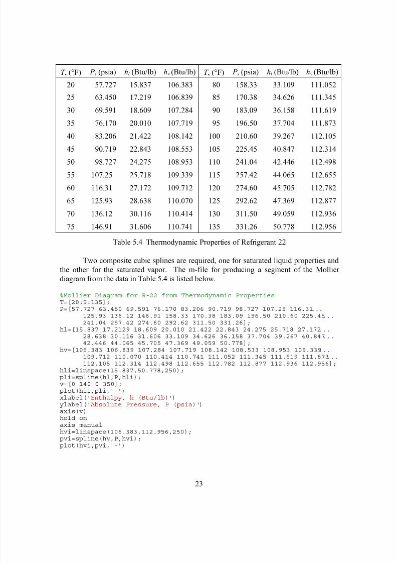
T , (°F) P , (psia) hl (Btu/lb) hv (Btu/lb) T , (°F) P , (psia) hl (Btu/lb) hv (Btu/lb)
20 57.727 15.837 106.383 80 158.33 33.109 111.052
25 63.450 17.219 106.839 85 170.38 34.626 111.34530 69.591 18.609 107.284 90 183.09 36.158 111.619
35 76.170 20.010 107.719 95 196.50 37.704 111.873
40 83.206 21.422 108.142 100 210.60 39.267 112.105
45 90.719 22.843 108.553 105 225.45 40.847 112.314
50 98.727 24.275 108.953 110 241.04 42.446 112.498
55 107.25 25.718 109.339 115 257.42 44.065 112.655
60 116.31 27.172 109.712 120 274.60 45.705 112.782
65 125.93 28.638 110.070 125 292.62 47.369 112.877
70 136.12 30.116 110.414 130 311.50 49.059 112.936
75 146.91 31.606 110.741 135 331.26 50.778 112.956
Table 5.4 Thermodynamic Properties of Refrigerant 22
Two composite cubic splines are required, one for saturated liquid properties and
the other for the saturated vapor. The m-file for producing a segment of the Mollier
diagram from the data in Table 5.4 is listed below.
%Mollier Diagram for R-22 from Thermodynamic PropertiesT=[20:5:135];P=[57.727 63.450 69.591 76.170 83.206 90.719 98.727 107.25 116.31... 125.93 136.12 146.91 158.33 170.38 183.09 196.50 210.60 225.45... 241.04 257.42 274.60 292.62 311.50 331.26];hl=[15.837 17.2129 18.609 20.010 21.422 22.843 24.275 25.718 27.172... 28.638 30.116 31.606 33.109 34.626 36.158 37.704 39.267 40.847... 42.446 44.065 45.705 47.369 49.059 50.778];hv=[106.383 106.839 107.284 107.719 108.142 108.533 108.953 109.339... 109.712 110.070 110.414 110.741 111.052 111.345 111.619 111.873... 112.105 112.314 112.498 112.655 112.782 112.877 112.936 112.956];hli=linspace(15.837,50.778,250);pli=spline(hl,P,hli);v=[0 140 0 350];plot(hli,pli,'-')xlabel('Enthalpy, h (Btu/lb)')ylabel('Absolute Pressure, P (psia)')axis(v)hold onaxis manualhvi=linspace(106.383,112.956,250);pvi=spline(hv,P,hvi);plot(hvi,pvi,'-')
8/13/2019 Interpolating Splines
http://slidepdf.com/reader/full/interpolating-splines 24/32
24
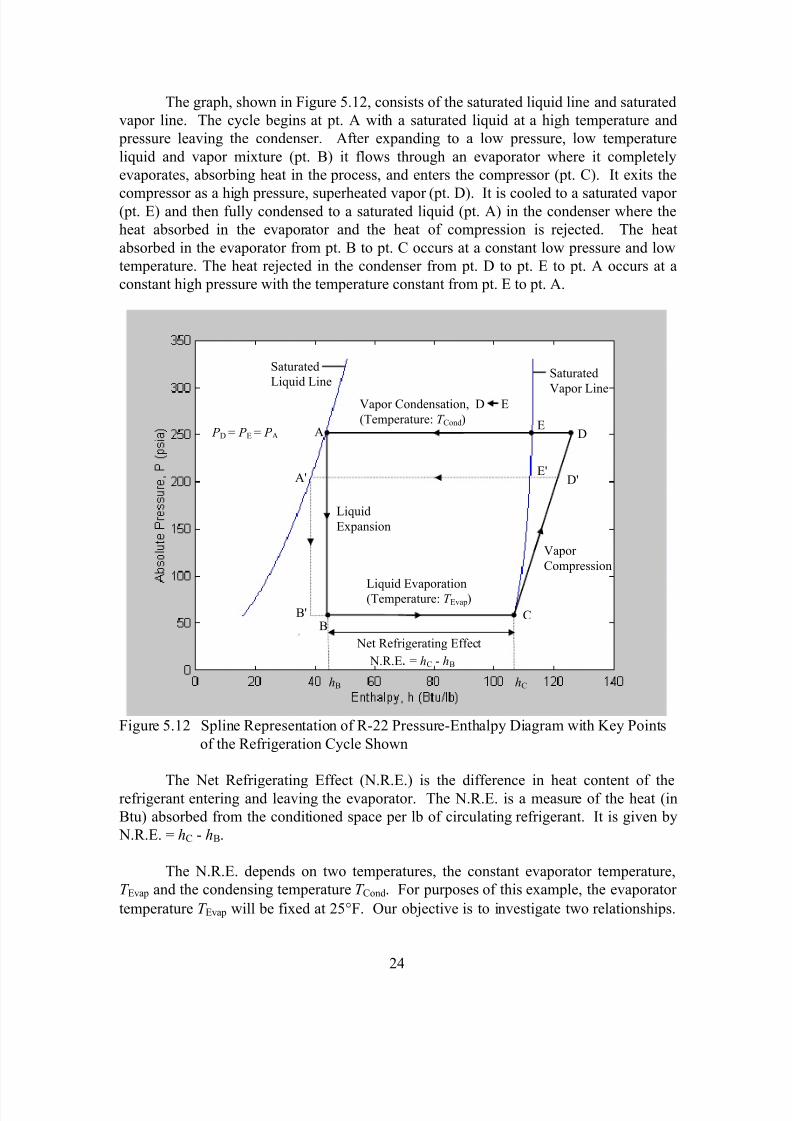
The graph, shown in Figure 5.12, consists of the saturated liquid line and saturated
vapor line. The cycle begins at pt. A with a saturated liquid at a high temperature and
pressure leaving the condenser. After expanding to a low pressure, low temperature
liquid and vapor mixture (pt. B) it flows through an evaporator where it completely
evaporates, absorbing heat in the process, and enters the compressor (pt. C). It exits the
compressor as a high pressure, superheated vapor (pt. D). It is cooled to a saturated vapor (pt. E) and then fully condensed to a saturated liquid (pt. A) in the condenser where the
heat absorbed in the evaporator and the heat of compression is rejected. The heat
absorbed in the evaporator from pt. B to pt. C occurs at a constant low pressure and low
temperature. The heat rejected in the condenser from pt. D to pt. E to pt. A occurs at a
constant high pressure with the temperature constant from pt. E to pt. A.
Figure 5.12 Spline Representation of R-22 Pressure-Enthalpy Diagram with Key Points
of the Refrigeration Cycle Shown
The Net Refrigerating Effect (N.R.E.) is the difference in heat content of therefrigerant entering and leaving the evaporator. The N.R.E. is a measure of the heat (in
Btu) absorbed from the conditioned space per lb of circulating refrigerant. It is given by
N.R.E. = hC - hB.
The N.R.E. depends on two temperatures, the constant evaporator temperature,
T Evap and the condensing temperature T Cond. For purposes of this example, the evaporator
temperature T Evap will be fixed at 25°F. Our objective is to investigate two relationships.
Net Refrigerating Effect
N.R.E. = hC - hB
A
BC
DE
Liquid Evaporation(Temperature: T Evap)
Vapor Condensation, D E
(Temperature: T Cond)
Liquid
Expansion
Vapor
Compression
SaturatedLiquid Line
Saturated
Vapor Line
hChB
P D = P E = P A
A'E'
D'
B'
8/13/2019 Interpolating Splines
http://slidepdf.com/reader/full/interpolating-splines 25/32
25
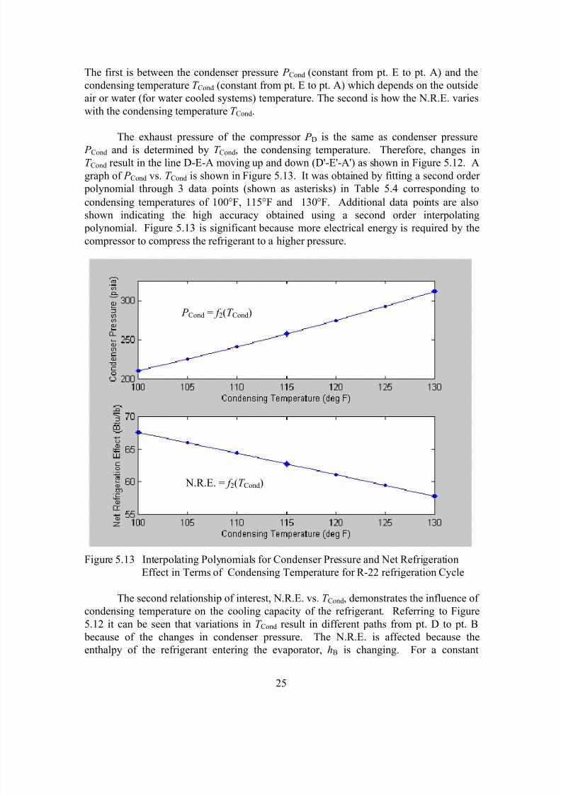
The first is between the condenser pressure P Cond (constant from pt. E to pt. A) and the
condensing temperature T Cond (constant from pt. E to pt. A) which depends on the outside
air or water (for water cooled systems) temperature. The second is how the N.R.E. varies
with the condensing temperature T Cond.
The exhaust pressure of the compressor P D is the same as condenser pressure P Cond and is determined by T Cond, the condensing temperature. Therefore, changes in
T Cond result in the line D-E-A moving up and down (D'-E'-A') as shown in Figure 5.12. A
graph of P Cond vs. T Cond is shown in Figure 5.13. It was obtained by fitting a second order
polynomial through 3 data points (shown as asterisks) in Table 5.4 corresponding to
condensing temperatures of 100°F, 115°F and 130°F. Additional data points are also
shown indicating the high accuracy obtained using a second order interpolating
polynomial. Figure 5.13 is significant because more electrical energy is required by the
compressor to compress the refrigerant to a higher pressure.
Figure 5.13 Interpolating Polynomials for Condenser Pressure and Net RefrigerationEffect in Terms of Condensing Temperature for R-22 refrigeration Cycle
The second relationship of interest, N.R.E. vs. T Cond, demonstrates the influence of
condensing temperature on the cooling capacity of the refrigerant. Referring to Figure
5.12 it can be seen that variations in T Cond result in different paths from pt. D to pt. B
because of the changes in condenser pressure. The N.R.E. is affected because the
enthalpy of the refrigerant entering the evaporator, hB is changing. For a constant
N.R.E. = f 2(T Cond)
P Cond = f 2(T Cond)
8/13/2019 Interpolating Splines
http://slidepdf.com/reader/full/interpolating-splines 26/32
8/13/2019 Interpolating Splines
http://slidepdf.com/reader/full/interpolating-splines 27/32
27
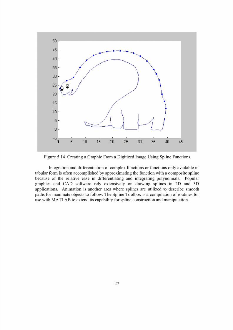
Figure 5.14 Creating a Graphic From a Digitized Image Using Spline Functions
Integration and differentiation of complex functions or functions only available in
tabular form is often accomplished by approximating the function with a composite spline because of the relative ease in differentiating and integrating polynomials. Popular
graphics and CAD software rely extensively on drawing splines in 2D and 3D
applications. Animation is another area where splines are utilized to describe smooth
paths for inanimate objects to follow. The Spline Toolbox is a compilation of routines for
use with MATLAB to extend its capability for spline construction and manipulation.
8/13/2019 Interpolating Splines
http://slidepdf.com/reader/full/interpolating-splines 28/32
8/13/2019 Interpolating Splines
http://slidepdf.com/reader/full/interpolating-splines 29/32
8/13/2019 Interpolating Splines
http://slidepdf.com/reader/full/interpolating-splines 30/32
8/13/2019 Interpolating Splines
http://slidepdf.com/reader/full/interpolating-splines 31/32
31
9. The graphs shown summarizes test results of a hermetic reciprocating compressor
using R-22 running at a constant speed. Capacity refers to the refrigeration effect that
can be achieved by the compressor. Power is the electrical power required by the
compressor motor.
Graphs for Problem 5.9
a) On a new set of graphs (one for Power and one for Capacity) plot the data points
and composite spline functions for each condensing temperature similar to the
dotted curves shown.
b) The EER (Energy Efficiency Ratio) of a refrigeration system is a measure of
performance defined as
EER = Capacity, in Btu / hrPower Input, in watts
Use the results of Part a) to prepare a set of performance curves (one for each
condensing temperature) relating the EER and the evaporating temperature.
c) Use the original set of data points to plot on separate graphs composite splines
curves of Capacity vs. Condensing Temperature and Power Input vs. Condensing
Condensing
Temperature = 130 °F
115 °F
100 °F
Condensing
Temperature = 100 °F
115 °F
130 °F

8/13/2019 Interpolating Splines
http://slidepdf.com/reader/full/interpolating-splines 32/32
Temperature. Each graph contains five curves corresponding to Evaporator
temperatures of 10 °F, 20 °F, 30°F, 40 °F and 50 °F.
d) Use the results of Part c) to prepare a set of performance curves (one for each
evaporating temperature) relating the EER and the condensing temperature.
10. Import a clip art graphic or scan a simple figure. Digitize it and represent it with a setof composite cubic splines. Display the original graphic and the cubic spline
representation along side each other.


![Chapitre II Interpolation et Approximation - unige.chhairer/poly/chap2.pdf · C. de Boor (1978): A Practical Guide to Splines. Springer-Verlag. [MA 65/141] G.D. Knott (2000): Interpolating](https://static.fdocuments.net/doc/165x107/5ab8f0ec7f8b9ac10d8d93e4/chapitre-ii-interpolation-et-approximation-unigech-hairerpolychap2pdfc-de.jpg)
![Rootsbender.astro.sunysb.edu/.../interpolation-roots.pdf · Cubic Splines Cubic splines: 3rd order polynomial in [x i, xi+1] – 1. Start by linearly interpolating second derivatives](https://static.fdocuments.net/doc/165x107/5f0661bf7e708231d417b6bd/cubic-splines-cubic-splines-3rd-order-polynomial-in-x-i-xi1-a-1-start-by.jpg)