Local Spatiotemporal Modelling of House Prices - …eprints.gla.ac.uk/107215/1/107215.pdf · Local...
31
1 Local Spatiotemporal Modelling of House Prices: A Mixed Model Approach Jing Yao 1* , A.Stewart Fotheringham 2 1 Urban Big Data Centre, School of Social and Political Sciences, University of Glasgow, Glasgow, G12 8RZ, UK. 2 GeoDa Centre for Geospatial Analysis and Computation, School of Geographical Sciences and Urban Planning, Arizona State University, Tempe, AZ 85281, USA. * Correspondence: Dr. Jing Yao Urban Big Data Centre School of Social and Political Sciences 7 Lilybank Gardens University of Glasgow Glasgow, UK G12 8RZ Phone: +44 (0) 141 330 2368 Email: [email protected] (JY), [email protected] (ASF)
Transcript of Local Spatiotemporal Modelling of House Prices - …eprints.gla.ac.uk/107215/1/107215.pdf · Local...

1
Local Spatiotemporal Modelling of House Prices:
A Mixed Model Approach
Jing Yao1*
, A.Stewart Fotheringham2
1Urban Big Data Centre, School of Social and Political Sciences, University of Glasgow,
Glasgow, G12 8RZ, UK.
2GeoDa Centre for Geospatial Analysis and Computation, School of Geographical Sciences
and Urban Planning, Arizona State University, Tempe, AZ 85281, USA.
*Correspondence:
Dr. Jing Yao
Urban Big Data Centre
School of Social and Political Sciences
7 Lilybank Gardens
University of Glasgow
Glasgow, UK G12 8RZ
Phone: +44 (0) 141 330 2368
Email: [email protected] (JY), [email protected] (ASF)

2
Local Spatiotemporal Modelling of House Prices:
A Mixed Model Approach
Abstract:
The real estate market has long provided an active application area for spatial-temporal
modelling and analysis and it is well known that house prices tend to be not only spatially
but also temporally correlated. In the spatial dimension, nearby properties tend to have
similar values because they tend to share similar characteristics but house prices tend to
vary over space due to differences in these characteristics. In the temporal dimension,
current house prices tend to be based on property values from previous years and in the
spatial-temporal dimension, the properties on which current prices are based tend to be in
close spatial proximity. To date, however, most research work on house prices has adopted
either a spatial perspective or a temporal one. Relative few efforts have been devoted to
the situation where both spatial and temporal effects coexist. Even fewer analyses have
allowed for both spatial and temporal variations in the determinants of house prices. Using
10-years of house price data in Fife, Scotland (2003-2012), this research applies a mixed
model approach, semi-parametric geographically weighted regression (GWR), to explore,
model and analyse the spatiotemporal variations in the relationships between house prices
and associated determinants. The study demonstrates the mixed modelling technique
provides better results than standard approaches to predicting house prices by accounting
for spatiotemporal relationships at both global and local scales.
Keywords: House price; Semi-parametric GWR; Spatiotemporal modelling; GIS

3
The real estate market has provided an active application area for both spatial and spatial-
temporal modelling and analysis (Meen 2001; Goodman and Thibodeau 2003; Bitter,
Mulligan, and Dall'erba 2007; Huang, Wu, and Barry 2010; Helbich, Vaz, and Nijkamp 2014;
Wu, Li, and Huang 2014). Unlike traditional hedonic price analysis, which usually attempts to
explain house prices in terms of property attributes, neighbourhood characteristics and
geographic locations through global models, spatial models in general explicitly account for
two major spatial effects in housing prices typically ignored in global models: spatial
dependency and spatial heterogeneity (Anselin 1988). The former refers to the similarity
commonly observed in the values of nearby properties whilst the latter indicates that the
processes generating house prices might vary over space, usually reflecting housing
submarkets or variations in household preferences (Bitter, Mulligan, and Dall'erba 2007).
Parameter estimates from traditional hedonic price models, which represent the
relationships between property prices and associated characteristics, can be biased in the
presence of spatial effects. As a result, extensive efforts have been devoted to incorporating
such spatial effects into hedonic house price analysis and many spatial statistical techniques
have been developed in the last a few decades (Anselin, Florax, and Rey 2004).
Several models applied in the spatial analysis of real estate data have been constructed to
address spatial dependence and/or spatial heterogeneity. Examples include spatial lag and
spatial error models (Anselin 1988; Can 1992; Dubin 1992), and geographically weighted
regression (GWR) (Fotheringham, Brunsdon, and Charlton 2002). Recently, spatiotemporal
models have been developed in order to incorporate the temporal dimension into hedonic
house price analysis as housing price processes evolve not only over space but also over
time (Case et al. 2004; Smith and Wu 2009; Huang, Wu, and Barry 2010; Wu, Li, and Huang
2014).
However, it is worth noting that both spatial effects (spatial dependence and spatial
heterogeneity) frequently coexist in many spatial processes (Anselin 1999) and there is
strong evidence indicating the presence of both spatial effects in the housing market
(Goodman and Thibodeau 2003). In this case, accurate parameter estimates cannot be
obtained from either global or local models which consider one effect in isolation from the
other. Instead, models capable of addressing both spatial effects become a desirable option.
To this end, of primary interest here is to understand both spatial effects in housing price
processes through the application of a mixed model method, semi-parametric GWR
(Fotheringham, Brunsdon, and Charlton 2002; Nakaya et al. 2005). Using a 10-year (2003 -
2012) house price dataset in Fife, Scotland, this research seeks to explore, model and
analyse spatiotemporal variations in house prices and their relationships with associated
determinants. Important in this study is the identification of which relationships tend to be
globally stable and which tend to vary over space, and whether spatial variations in house
price determinants are temporally stable.

4
The remainder of the paper is organized as follows. The subsequent section provides a
review of spatial statistical approaches for housing price research. This is followed by a
description of a 10-year house price dataset in Fife, Scotland. Then, the application of semi-
parametric GWR to examine both temporal and spatial variations in the determinants of
house prices is described. The paper concludes with the major findings and the significance
of this research.
Spatial Hedonic Models for House Price Analysis
Hedonic price analysis has long been widely applied in property assessment (Can 1992;
Meen 2001; Fotheringham, Brunsdon, and Charlton 2002). In general, hedonic price
modelling relates the value of goods to a set of their characteristics (Goodman 1998). In real
estate studies, hedonic house price models aim to estimate the market value of properties
based upon a set of associated characteristics which generally include structural attributes
(e.g. number of rooms, floor area and dwelling age), neighbourhood attributes (e.g. quality
of public education, unemployed rate and racial diversity) and locational attributes (e.g.
proximity to workplaces, accessibility to pleasant landscapes and public facilities) (Basu and
Thibodeau 1998). Then property prices can be defined as a function of the above three basic
categories of characteristics, which can be expressed as:
p = f(S, N, L) (1)
Where p represents property price; S represents a set of variables describing structural
attributes of the property; N represents a set of neighbourhood characteristics; and L
represents a set of location attributes The function f is usually expressed in a traditional
linear regression form and calibrated using ordinary least squares (OLS) technique.
However, as mentioned, the hedonic price model in (1) typically ignores the spatial effects
commonly existing in housing prices. The awareness of limitations of traditional hedonic
price analysis has led to a wide range of models accounting for spatial effects in residential
datasets (Tse 2002; Farber and Yates 2006; Bitter, Mulligan, and Dall'erba 2007; Helbich, Vaz,
and Nijkamp 2014). In general, such models can be considered global or local according to
whether they deal with spatial dependency or spatial heterogeneity. The remainder of this
section provides a brief review of two types of models as well as their applications in
housing price analysis.
Global spatial models address spatial dependence or spatial autocorrelation in spatial
processes. A comprehensive discussion of well-known such models can be found in Anselin
(1988), Haining (1990), Anselin, Florax, and Rey (2004) and LeSage and Pace (2009). For
example, the widely utilized specification provided by Anselin (1988) assumes spatial
autocorrelation is in either the response variable or the error terms, and the corresponding
models are usually calibrated by maximum likelihood (ML) rather than OLS technique as
some OLS assumptions (e.g. independently and identically distributed residuals) are violated.

5
Unlike the spatial lag or error model, Tse (2002) specified spatial autocorrelation through
the constant term using a stochastic approach.
In addition to the spatial dimension, dependence in time has also received much research
interest. For instance, Pace et al. (2000) formulated a spatiotemporal autoregression model
and applied it in a study of housing prices in Baton Rouge, Louisiana, by modelling both
spatial and temporal dependence in the errors. Gelfand et al. (2004) proposed a class of
spatiotemporal hedonic models under a Bayesian statistical framework and examined the
spatiotemporal differences related to single versus multiple residential sales. Smith and Wu
(2009) developed a spatiotemporal model allowing for both spatial and temporal lag effects,
which was applied to study housing price trends in the Philadelphia area, USA.
Although these global spatial models represent a substantial improvement over traditional
hedonic models, a major issue is that the housing price processes are assumed to be
constant or stationary over space, which is not necessarily the case in reality. In order to
capture spatial variations in housing price processes, numerous local spatial models have
been proposed. Common local models include the spatial expansion method (Casetti 1972),
moving window regression (MWR) (Farber and Yeats 2006), multilevel models (Duncan and
Jones 2000) and geographically weighted regression (GWR) (Fotheringham, Brunsdon, and
Charlton 2002). These can be considered to be generalizations of standard linear models,
where parameter estimates are allowed to vary over space in order to better represent the
processes generating house prices (Fotheringham, Brunsdon, and Charlton 2002). For
example, Farber and Yeats (2006) found GWR outperformed other local modelling
approaches with regard to explaining spatial variations in housing prices in a study of the
real estate market in Toronto, Canada. Similarly, Bitter, Mulligan, and Dall'erba (2007)
compared two local models, the spatial expansion method and GWR, in a research of
housing market in Tucson, Arizona, USA, concluding that GWR is superior in terms of the
capability of identifying spatial heterogeneity in several housing attributes. Páez, Long, and
Farber (2008) compared MWR, GWR, and the moving windows Kriging (MWK) approaches
in relation to different spatial effects, highlighting the importance of market segmentation
in housing price processes.
Beyond space, time has also been incorporated into local models to account for temporal
effects on housing processes. For example, Crespo (2009) and Huang, Wu, and Barry (2010)
extend traditional GWR to a spatiotemporal GWR (GTWR) by developing a spatiotemporal
kernel function in local model calibration. Wu, Li, and Huang (2014) further extended GTWR
by accounting for auto-correlated effects.
It can be seen, from the discussion above, that existing global and local spatial models are
both extensive and diverse. Empirical applications in real estate markets in various spatial
settings have shown their effectiveness in explaining spatial dependence or spatial
heterogeneity. In contrast, mixed models dealing with both spatial effects have received less
attention, particularly for hedonic house price analysis. This research will contribute to the

6
literature by utilizing a mixed model, semi-parametric GWR, to investigate both global and
local relationships between house prices and associated influencing factors, as well as their
variations over time.
Data and Study Area
The data used in this research are provided by Registers of Scotland (ROS) and consist of
sales prices for houses during 2003-2012 in Fife, Scotland. Fife is located in southeast
Scotland as shown in Figure 1 and it covers an area about 1,325 km2 with a population
around 276/km2 (estimated in 2012). St Andrews, a historic town renowned as the “home of
golf”, is on the northeast coast. It is also home to the University of St Andrews which
generates a high demand for accommodations and creates a distinctive local housing
market.
Figure 1 about here
The geographical data are geo-referenced points defined by (x, y) coordinates representing
the spatial location of houses. Each house has an associated attribute – property value – at
the time of transaction. Figure 2 depicts the spatial distribution of house prices for 2012,
where the points in Figure 2A represent the location of houses with the heights indicating
the relative property values. Shown in Figure 2B is a continuous surface generated from
those points, from which the general spatial pattern of house prices can be observed.
Residences in the north east coast, mainly clustered around St Andrews, tend to be more
expensive than those in rests of Fife. Another area having higher house prices is around
Dunfermline, the 2nd largest town by population in Fife. All the other areas, in contrast, have
relatively lower house prices.
Figure 2 about here
Table 1 summarizes the number of houses sold in each year, the mean house price and the
inflation-adjusted mean house price. The number of houses sold peaked in 2006 and then
declined rapidly, leading to and following from the economic crash in 2008. Inflation-
adjusted house prices peaked in 2008 and declined each year thereafter. As after 2007 the
average number of sales per zone drops to about 10, one concern here is about the
potential impact of houses per zone on the validity of the zonal average. However, over the
study time period (2003-2012), more than 90% of data zones contain <40 properties. Also,
the average house prices on each data zone largely have similar distribution over time for
the zones containing <40 properties. Thus, the number of houses per zone should not have
great impacts in terms of model calibration.
Table 1 about here
7
Since the structural characteristics for each property are not available, relevant socio-
economic data were obtained from the Scottish Neighbourhood Statistics (SNS)1 in order to
help understand the underlying housing price processes. These data are summarized
statistics on small-area statistical geographies – data zones –which are nested within local
authority boundaries and have a population of 500 – 1,000 household residents. In total
there are 453 data zones in Fife. Accordingly, house prices are also aggregated to derive the
average house prices for each data zone.
In the subsequent regression analysis, the dependent variable is the average house price
within each of the 453 data zones and the definition of the covariates, X, are presented in
Table 2. In addition to neighbourhood characteristics such as population density and crime
rates, and property mix variables, two spatial variables, “distance to St Andrews” and
“distance to coast”, are considered given the spatial context in the study area. The former
accounts for the potential effects from the historic town St Andrews and the latter
recognizes buyers’ preference for sea view properties. Also, given the spatial and temporal
dependences commonly existing in house prices, a spatiotemporal lag variable is added to
the model. A spatial lag can be calculated as the average house price of the neighbours
(Anselin 1988). A spatiotemporal lag is therefore defined as the average house price of the
neighbours in the previous year. In this case, the spatiotemporal lag is first calculated on
neighboring houses and then aggregated at the data zone level.
Table 2 about here
Methods
This research investigates spatiotemporal variations in housing prices using a mixed spatial
model, semi-parametric GWR (Fotheringham, Brunsdon, and Charlton 2002; Nakaya et al.
2005), which is an extension of a local spatial modelling technique, traditional GWR
(Fotheringham, Brunsdon, and Charlton 2002). In this case, semi-parametric GWR is utilized
to examine both global and local spatial relationships between house prices and a set of
associated attributes for each year and the temporal variations in the coefficients are
obtained through a series of independent cross-sectional estimations. In addition, the
performance of three models, the traditional global model, GWR and semi-parametric GWR
is compared.
Before defining semi-parametric GWR, it is helpful to first describe a traditional global
hedonic model and traditional GWR in the context of housing market studies. A global
hedonic house price model can be formulated as in (2):
∑ (2)
1 http://www.sns.gov.uk/

8
where i and j are index of observations and covariates, respectively; P represents house
prices; X represents covariates; and represents parameters associated with the various
covariates. According to (2), the parameter is constant across all observations. That is, the
relationship between the jth covariate and house prices is considered invariant over space.
In contrast, such relationships are allowed to vary across space in GWR which can be
expressed in (3):
∑ (3)
where ) represents the geographic location of the ith observation. Thus, the
parameter is a function of ), denoted as . The local parameters are
estimated with the aid of data in the neighbourhood, which is usually realized by a weight
matrix. Commonly, the weights are defined by Gaussian or bi-square kernel functions where
the size of neighbourhood is determined by an optimised bandwidth (e.g. distance or
number of nearest neighbours) (Fotheringham, Brunsdon, and Charlton 2002). As a result,
smaller bandwidths indicate more local processes whereas larger bandwidths indicate more
regional processes with a bandwidth tending to infinity replicating a global model.
Built upon the above formulations, the semi-parametric GWR model can be defined as in (4):
∑ ∑ (4)
where k is an index of covariates that have a global relationship with house prices and j is
an index of covariates whose relationship to house prices varies spatially. Thus, semi-
parametric GWR allows some parameters to be fixed over space and the other parameters
to vary across space, representing stationary and non-stationary spatial
relationships/processes simultaneously. The model in (4) is usually calibrated using an
iterative procedure by estimating global and local parameters in turn repeatedly until some
convergence condition is satisfied (Fotheringham, Brunsdon, and Charlton 2002; Nakaya et
al. 2005).
In this research, the semi-parametric GWR model in (4) is used to study the 10-year house
price dataset in Fife, Scotland. The aggregated house prices and all the values of covariates
are transformed using the natural logarithm function to ensure the parameter estimation is
free from scale effects. In other words, the particular mixed hedonic house price model in
this research is defined as in (5):
∑ ∑ (5)
There are two important issues involved in the calibration of model (5). First, a bandwidth
needs to be determined for the weight matrix construction. Also, variables need to be
selected as global or local. In this research, a bi-square kernel function is used to define the
weight matrix with the bandwidth specified by the number of nearest neighbours. The
optimal bandwidth size is chosen such that the corresponding model has the smallest value

9
for the corrected Akaike information criterion (AICc) (Akaike 1974). AICc is widely applied in
model selection with smaller values indicating better models. This procedure is repeated for
annual house price data to ensure the best model is found for each year. The second issue is
addressed by a local to global variable selection routine which can be summarized as follows:
Step 1. Define two sets of variables, G and L, and initialize G = , and L contains all
the variables. That is, L = {x1, x2, …, x13}. Construct a GWR model defined in (3)
using variable sets G and L. Denote this model as model_old;
Step 2. Solve model_old and get the corresponding AICc, recorded as AICc_old;
Step 3. Take a variable, e.g. xi, out of set L and put it into set G. Construct a semi-
parametric GWR using the variables defined by L and G. Denote this model as
model_new;
Step 4. Solve model_new and get the corresponding AICc, recorded as AICc_new;
Step 5. If AICc_new < AICc_old, keep xi in G and let AICc_old = AICc_new; otherwise,
put xi back to L;
Step 6. Repeat Step 3 – Step 5, until every variable in L is examined;
Step 7. If there is at least one variable moved from L to G during Step 3 – Step 6,
repeat Step 3 – Step 6; otherwise, stop.
It is worth noting that an optimal bandwidth search is implicitly contained in each model
calibration procedure, which further complicates the above variable selection because more
computation processing is required. The bandwidth search, variable selection and
parameter estimation involved in model (5) are all carried out in GWR 42, a package for local
spatial modelling and analysis.
Once the parameter estimates are derived, it is critical to assess whether the measured
relationships between house prices and associated determinants are intrinsically differences
across space or simply caused by random sampling variations. This is carried out through
stationarity tests of each local parameter in the semi-parametric GWR models. Specifically,
two approaches are employed here: variability tests of local parameter estimates and
Monte-Carlo (MC) tests (Fotheringham, Brunsdon, and Charlton 2002). The former is based
on the inter-quartile range (IQR) of local estimates and the standard errors (SE) of global
estimates. Empirically we can consider the 2*SE as the expected variations in the values as it
contains about 60% of all the estimates. Thus, it indicates a possible non-stationary process
if IQR (which includes 50% of values) is larger than 2*SE. The latter measures the variance of
the local parameters, which can be defined as in (6):
2 http://www.st-andrews.ac.uk/geoinformatics/gwr/gwr-software/

10
∑ (
∑ )
(6)
where is the variance of the jth parameter; n is the total number of observations; is
the local estimate for observation i and parameter j. The MC tests are implemented in the
following steps:
Step 1. Obtain local parameter estimates and calculate for each local parameter;
Step 2. Rearrange data randomly across the zones (keeping Yi and Xi) together;
Step 3. Compute a new set of local parameter estimates based on the rearranged
data and calculate ;
Step 4. Repeat steps 2 and 3 for N times, each time computing the variance of the
local estimates;
Step 5. Compare the variance of local parameter estimates in step 1 with those from
steps 2 and 3;
Step 6. The p value associated with step 1 is then the proportion of variances that lie
above that for step 1 in a list of variances sorted high to low.
If there is no significant pattern in the parameters, there should be no significant changes in
the variations in the local estimates regardless of the permutation of the observations
against their locations. As it is difficult to obtain the null distribution of the variance
analytically, the MC method is commonly considered an effective option. Thus, N values of
the variance of a parameter obtained from the MC test represent an experimental
distribution, and a p value (experimental significance level) can be derived by comparing the
actual value of the variance against that list of N values. Generally, IQR test is quite easy and
straightforward but is more informal. In contrast, MC test is more rigorous but limited in
repetitions due to computational time.
Finally, the coefficient of variation (CV) is employed to investigate the spatiotemporal
variations of local parameter estimates. Specifically, a CV is calculated using the local
estimates for each year, from which a set of CVs can be derived to demonstrate the spatial
variations in the relationships between house prices and the covariates over time. Also, a CV
is calculated for each data zone based on the local estimates across the study period (2003-
2012), from which the temporal variations in the relationships between house prices and
the covariates over space can be generated.
Results
For the purpose of model comparison, global models, GWR models as well as semi-
parametric GWR models are fitted in this research. First, a global model is calibrated to

11
explore the general relationships between house prices and the associated attributes. Then,
results from the semi-parametric GWR model are presented, including estimates for fixed
and local parameters with spatiotemporal variations in local parameter estimates
highlighted. Finally, the performances of different models are compared using a common
model selection criterion AICc.
Parameter estimates for the global model are given by Table 3. In total, nine models are
calibrated using OLS for the years 2004 – 2012 because the spatiotemporal lag is not
available for year 2003. It should be noted that the spatial lag in this case is temporal and
excludes the properties from the current year on the RHS in (5). Thus, it is appropriate to
use OLS for estimating the spatiotemporal lag parameter. According to the R2 (around 0.7),
the overall model fit is quite satisfactory for every year except 2007 (R2 = 0.38). Seven
variables have reasonably consistent significant effects on house prices: x1 (population
density), x7 (% of dwellings with 1-3 rooms, i.e. small houses), x8 (% of dwellings with 7-9
rooms, i.e. big houses), x9 (% of household ownership), x11 (distance to St Andrews), x12
(distance to coast) and x13 (spatiotemporal lag). For example, the value of varies from -
0.074 (2007) to -0.040 (2004), which indicates that house prices tend to be lower, ceteris
paribus, in areas of higher population density. This effect strengthened up to 2007 and
thereafter has weakened. Similarly, according to the values of (-0.088 ~ -0.157), the
properties tend to have higher values the closer they are to St Andrews, ceteris paribus. In
contrast, some variables almost have no significant effects on house prices at all except for a
particular year, such as x2 (% of pensionable age population), x3 (% of working age
population) and x4 (% of semi-detached properties). The impacts of the other variables are
inconsistent.
Table 3 about here
Figure 3 describes the temporal variations in the seven consistently significant parameter
estimates. It can be seen that the estimates are reassuringly consistent over time with the
exception of the estimates associated with the variables x9 (% of household ownership) and
x13 (spatiotemporal lag) which both show a pronounced spike in value in 2007 as the
economic crisis loomed.
Figure 3 about here
The best semi-parametric GWR model is chosen for each year based on the variable
selection procedure described in the previous section. This produces for each year a set of
spatially varying parameter estimates for those variables whose effect on house prices
varies over space and a set of spatially invariant estimates for those variables whose effect
on house prices is constant over space. In each year only one or two variables appear to
have a constant impact on house prices with the exception of 2006 and 2007 with 4 and 5
parameters being fixed over space. There was no consistency in which variables exhibited a
fixed effect over time.

12
With regard to the local parameters, two tests were undertaken to identify if the spatial
variation in their values was significant. For each year, tests based on IQR of local estimates
and MC simulation (with repetition N=10003) are implemented. The results are shown in
Table 4. As can be seen, different sets of significant local parameters are found for each year.
In general, the local parameters specified by the local to global variable selection routine
described in Section 4 do not all have significant local variability. For example, for year 2004,
the variable selection routine suggests that only x1 (population density) is fixed while the
IQR test indicates the estimates for another three parameters do not significantly vary
across space: x5 (% of terraced properties), x6 (% of flats) and x8 (% of dwellings with 7-9
rooms) and the MC test suggests only four sets of parameter estimates exhibit significant
spatial variation – , , and .
Generally, the results of the IQR and the MC tests are reassuringly similar and where
discrepancies exist, the MC test appears to be more rigorous. Three variables exhibit
significant spatial variation in their impact on house prices throughout the 9 time periods.
These are distance to St Andrews, distance to the coast and the spatial-temporal lag variable.
Interestingly, crime rates appear to have a spatially varying impact on house prices up to
2008 but thereafter do not exhibit any significant spatial variation. The remaining variables
exhibit no consistency in the significance of the spatial variation of their effects.
Table 4 about here
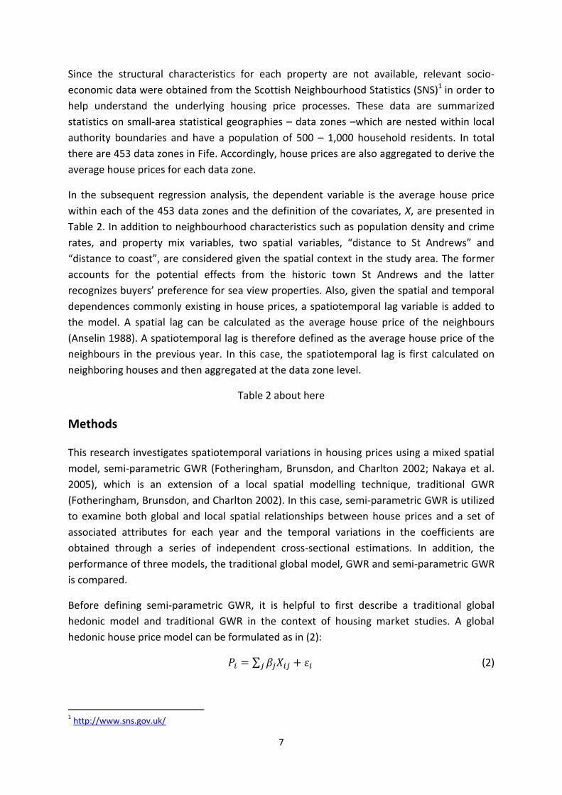
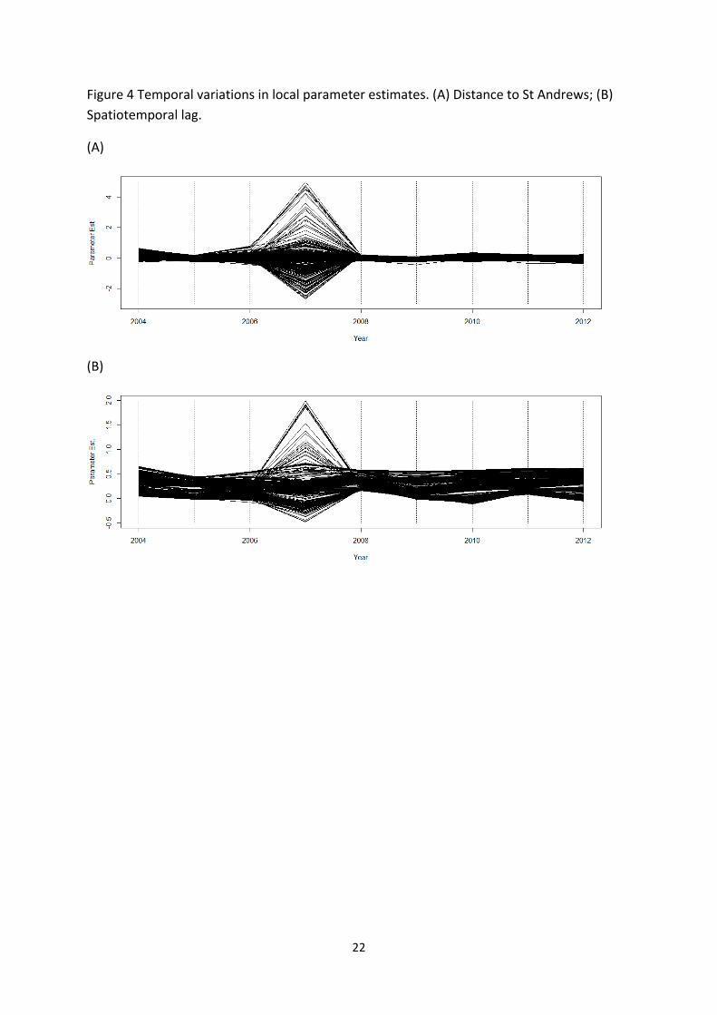
Accordingly, two variables x11 (distance to St Andrews) and x13 (spatiotemporal lag) are
selected for further discussion here because they generally exhibit significant variation in
the local estimates. For each variable and for each year, there are 453 local parameter
estimates describing the impact of that variable on house prices in the vicinity of location i
in time t. In Figure 4 the values of each of the 453 estimates across the 9 time periods is
connected by a straight line across the 9 time periods. This is done separately for the
parameter estimate associated with the variable “Distance to St Andrews” and the
parameter estimate associated with the spatiotemporal lag variable. The local parameter
estimates show remarkable consistency through time but the most noticeable feature is
that for the year 2007, the local parameter estimates exhibit a vastly increased spatial
variation. This is the year leading to the housing-led economic crisis when presumably the
housing market was in the throes of impending turmoil. It is very interesting that this is
exhibited in advance of the full-blown crisis being recognised and the turmoil in the
determination of house prices is only for this one time period and not for the full period of
the crisis.
Figure 4 about here
3 We use N=1000 because of the computational complexity. We also run the MC test with N=100 which gave similar results as those from N=1000, which indicates the MC test is rigorous.

13
To examine this effect further, the local parameter estimates for these two variables are
mapped for each of the nine periods as shown in Figure 5. However, to aid clarity, only
those local parameter estimates which were significant are depicted. In this case,
significance is defined using the adjusted critical t value (Byrne, Charlton, and Fotheringham
2009) equated with an original significance level of 0.05, which addresses the issue of
multiple hypothesis testing in GWR.
Figure 5 about here
Figure 5A depicts the significant local parameter estimates for the variable “Distance to St
Andrews”. These are all negative indicating the region around St Andrews where house
prices fall as distance to St Andrews increases, cateris paribus. In effect, these maps indicate
the spatial extent of the local St Andrews housing market in each time period. In general
there is remarkable consistency over time in this housing market with the exception of 2007
when it disappears altogether and in 2012 when the southern portion disappears. In 2007,
the location of St Andrews had no effect on house prices anywhere in Fife. In 2012 it had an
impact only on those houses in an area to the north and west of the city. In other years the
area of impact is consistently the whole of north-east Fife with a radius of approximately
20kms from St Andrews. This technique this usefully quantifies the spatial extent of the
housing market around an urban area and could easily be extended to other features
deemed to have an impact on house prices such as airports or pollution sites.
Figure 5B depicts the spatial extent of neighbourhood effects in housing prices which are
consistently significant only in the north-east half of Fife. The only exception to this again is
the year 2007 when very little spatial lag effect is present anywhere in the county. The
interpretation of this is that house prices are strongly related to neighbouring house prices
only in the north-east of Fife – in the rest of the county, there is no spatial lag affect present
in house prices. This may indicate again two very different housing regimes in the county
and indeed, north-east Fife is quite different economically and socially from south-west Fife.
In addition, the extent to which the local estimates vary over space and time is also explored
using the CV mentioned previously. Take the variable “spatiotemporal lag” as an example,
Figure 6 shows the spatial variation of the CVs over time, where a CV is calculated for the
453 local estimates for every year. It can be seen that the value in 2007 is much higher than
those in all the other years, indicating unusual spatial variation in the neighbourhood effects
on house prices as observed in Figure 4B. Interestingly, in 2008 when the financial crisis
occurred, the CV has the lowest value compared those in the other years. Further, the
temporal variation of the CVs for the same variable is shown in Figure 7. In general, the
values gradually decline towards southwest Fife, indicating decreasing temporal variations
in neighbourhood effects. Also noteworthy is that north Fife has the relatively fewer
temporal variations in the local estimates which, as shown in Figure 5B, are consistently
significant across the study time period (except 2007).

14
Figure 6 about here
Figure 7 about here
Finally, a model comparison is undertaken out based on the AICc values as shown in Table 5.
The AICc values cannot be compared across years but for each year, the lower the AICc, the
better the model fit with differences of 3 or more generally deemed to indicate a significant
difference. For all 9 time periods semi-parametric GWR consistently outperforms GWR
which in turn is superior to the global model, implying improvements in modelling both
global and local relationships underlying housing price processes.
Table 5 about here
Discussion and Conclusions
It is well known that housing markets are characterized by both spatial dependence and
spatial heterogeneity. The literature on spatial hedonic house price analysis so far has
largely focused on either global models or local models and has either ignored both effects
or treated them independently. This research accounts for both spatial effects in housing
markets using a mixed model method, semi-parametric GWR. Particularly, spatiotemporal
variations in neighbourhood effects (i.e. spatial dependence) on housing prices are
investigated. The results demonstrate that semi-parametric GWR is capable of dealing with
both global and local spatial relationships and therefore can produce more accurate
estimates for parameters in hedonic house price models.
The most important contribution of this research is the specification of both global and local
relationships between housing prices and the associated covariates, as well as their
variations over both space and time. For example, the spatial/temporal lag is widely used in
the global models and the extent of neighbourhood effects are traditionally considered
invariant over space. This is reflected in Table 3 where the coefficients of spatiotemporal lag
are all positive across the study time period. In fact, such neighbourhood effects can vary
over space and time, which is revealed by Figure 5B. That is, only the prices of the
residences in north eastern Fife are significantly affected by their neighbours’ prices and
such effects tend to increase from the northwest to the northeast. Meanwhile, the global
parameters also have changed over time. For example, population density is found
negatively related to housing prices in the global models (Table 3) but the mixed models
suggest that this only holds for years 2004, 2007, 2008 and 2011, and the regression
coefficients are only significant for year 2008.
Also worth noting is that this technique has quantified a local housing market effect – in this
case on the basis the effect of distance to St Andrews has on house prices. St Andrews is
the location of the University of St Andrews and has the unique features such as being the
home of the Royal and Ancient Golf Club. Given the consistent high accommodation

15
demand, St Andrews has formed a distinct housing market and the housing prices are
usually higher than those in other areas. Figure 5A describes the spatial extent of this effect.
That is, generally only the houses up to 20km away from St Andrews are subject to such an
effect in terms of housing prices. This technique could easily be expanded to other urban
centres to compare their impact on house prices and to other features such as airports and
landfill sites which are suspected to cause decreases in house prices but to what distance is
largely unknown.
Another interesting finding is the distinction of spatiotemporal patterns before and after the
financial crisis. As is well known, the residential real estate markets suffered greatly from
the financial and economic crisis in 2008. This is reflected in Table 1 where the housing
prices have an increasing trend before 2008 and a declining trend afterwards. Particularly,
based on the unusual parameter estimates from both the global model (Table 3 and Figure 3)
and the mixed model (Figures 4, 5 and 6), it would appear that the housing market in 2007
had detected some signs of the coming crisis and house prices in that year suddenly became
much less predictable. Furthermore, Figures 5B suggest quite different spatial distributions
of significant local estimates before and after the financial crisis. One concern here is that
the “breakdown” of parameter estimates in 2007 might be caused by the covariates as
different sets of coefficients are held constant in different years in the semi-parametric
GWR models. This is further investigated by the variations in local estimates obtained from
GWR, particularly for the two variables “Distance to St Andrews” and “Spatiotemporal lag”.
The results from GWR are very similar to those shown in Figures 4 and 5, which suggest the
covariates in semi-parametric GWR, particularly the fixed variables, have little impacts on
the variations in local estimates.
One limitation of this research is that both housing prices and associated influencing
characteristics are aggregated data based on data zones. It is well recognized that analyses
using aggregated data are subject to the choice of geographic units, and the resulting
conclusions might conceal the detailed information for underlying individual objects, which
is known in geography as the modifiable area unit problem (MAUP) (Openshaw, 1984).
Nevertheless, given that data zones are the only available geographic districts containing
local statistics and they have reasonable sizes (covering 500 – 1,000 household residents),
conclusions from this research still can provide useful insights regarding the general
spatiotemporal patterns in housing prices and social-economic factors.
In summary, housing market remains a great concern of government, real estate developers
and general population as it is a main component of macro-economy and also closely
related to social equity. GIS based spatial analysis, particularly spatial statistics, offers a set
of powerful tools to study housing price processes by explicitly accounting for spatial
dependency and spatial heterogeneity. This research demonstrates the advantages of a
mixed model method, semi-parametric GWR, in modelling both spatial effects as well as
both global and local relationships in housing price processes.

16
Though semi-parametric GWR in this research has been used to study the spatiotemporal
variations in the local housing market in Fife, Scotland, it can be employed in a wider field of
hedonic price modelling wherever both global and local spatial relationships are of concern.
Undoubtedly, semi-parametric GWR offers an effective way for spatial analysis and
modelling by its capability of capturing both spatial stationary and non-stationary processes.
References
Akaike, H. 1974. A new look at the statistical model identification. IEEE Transactions on
Automatic Control 19 (6): 716–723.
Anselin, L. 1988. Spatial Econometrics: Methods and Models. Kluwer Academic Publishers,
Dordrecht, The Netherlands.
Anselin, L. 1999. Spatial econometrics. In: A Companion to Theoretical Econometrics, ed. B.H.
Baltagi, 310–330. Oxford: Blackwell.
Anselin, L., Florax, R. J., and Rey, S. J. 2004. Advances in Spatial Econometrics. Methodology,
Tools and Applications. Berlin: Springer-Verlag.
Basu, S. and Thibodeau, T.G. 1998. Analysis of spatial autocorrelation in house prices.
Journal of Real Estate Finance and Economics 17(1): 61-85.
Bitter, C., Mulligan, G.F., and Dall’erba, S. 2007. Incorporating spatial variation in housing
attribute prices: a comparison of geographically weighted regression and the spatial
expansion method. Journal of Geographical Systems 9(1): 7–27.
Byrne, G., Charlton, M., and Fotheringham, A.S. 2009. Multiple dependent hypothesis tests
in geographically weighted regression. Paper presented at the 10th International
Conference on GeoComputation, Sydney, Australia, November 30-Decemeber 2, 2009.
Can, A. 1992. Specification and estimation of hedonic housing price models. Regional
Science and Urban Economics 22(3): 453-474.
Case, B., Clapp, J., Dubin, R., and Rodriguez, M. 2004. Modeling spatial and temporal house
price patterns: a comparison of four models. Journal of Real Estate Finance and
Economics 29(2): 167–191.
Casetti, E. 1972. Generating models by the expansion method: applications to geographic
research. Geographical Analysis 4: 81–91.
Crespo, R. 2009. Statistical Extensions of GWR: Spatial Interpolation and a Spatiotemporal
Approach. PhD thesis, National Centre for Geocomputation, University of Ireland,
Maynooth.

17
Dubin, R.A. 1992. Spatial autocorrelation and neighborhood quality. Regional Science and
Urban Economics 22: 432–452.
Duncan, C. and Jones, K. 2000. Using multilevel models to model heterogeneity: potential
and pitfalls. Geographical Analysis 32: 279-305.
Farber, S. and Yates, M. 2006. A Comparison of Localized Regression Models in a Hedonic
Price Context. Canadian Journal of Regional Science 29(3): 405-419.
Fotheringham, A.S., Brunsdon, C. and Charlton, M. 2002. Geographically weighted
regression: the analysis of spatially varying relationships. Chichester: Wiley.
Gelfand, A.E., Ecker, M.D., Knight, J.R., and Sirmans, C.F. 2004. The dynamics of location in
home prices. Journal of Real Estate Finance and Economics 29, 149–166.
Goodman, A.C. 1998. Andrew Court and the invention of hedonic price analysis. Journal of
Urban Economics 44(2): 291-298.
Goodman, A.C. and Thibodeau, T.G. 2003. Housing market segmentation and hedonic
prediction accuracy. Journal of Housing Economics 12(3): 181-201.
Haining, R. 1990. Spatial Data Analysis in the Social and Environmental Sciences. Cambridge
University Press, Cambridge.
Helbich, M., Vaz, E., and Nijkamp, P. 2014. Spatial Hedonic Models to Estimate Single Family
Home Prices in Austria. Urban Studies 51(2): 390-411.
Huang, B., Wu, B., and Barry, M. 2010. Geographically and temporally weighted regression
for modelling spatio-temporal variation in house prices. International Journal of
Geographical Information Science 24(3): 383-401.
LeSage, J.P. and Pace, R.K. 2009. Introduction to Spatial Econometrics. CRC Press, Boca Raton,
FL.
Meen, G. 2001. Modelling Spatial Housing Markets: Theory, Analysis and Policy. Boston:
Kluwer Academic Publishers.
Nakaya, T., Fotheringham, A.S., Brunsdon, C., Charlton, M. 2005. Geographically weighted
Poisson regression for disease association mapping. Statistics in Medicine 24(17), 2695-
2717.
Openshaw, S. 1984. The Modifiable Areal Unit Problem. CATMOG, 38. Norwich, England:
Geobooks.
Pace, R.K., Barry, R., Gilley, O.W., and Sirmans, C.F. 2000. A method for spatial–temporal
forecasting with an application to real estate prices. International Journal of Forecasting
16: 229-246.

18
Páez, A., Long, F., and Farber, S. 2008. Moving window approaches for hedonic price
estimation: an empirical comparison of modeling techniques. Urban Studies 45(8):
1565–1581.
Smith, T.E. and Wu, P. 2009. A spatio-temporal model of housing prices based on individual
sales transactions over time. Journal of Geographical Systems 11: 333–355.
Tse, R.Y.C. 2002. Estimating neighbourhood effects in house prices: towards a new hedonic
model approach. Urban Studies 39: 1165–1180.
Wu, B., Li, R., and Huang, B. 2014. A geographically and temporally weighted autoregressive
model with application to housing prices. International Journal of Geographical
Information Science 28(5): 1186-1204.

19
Figure 1 Study area: Fife, Scotland

20
Figure 2 Spatial distributions of house prices in 2012. (A) Discrete point; (B) Continuous
surface.
(A)
(B)

21
Figure 3 Temporal variations in global parameter estimates
22
Figure 4 Temporal variations in local parameter estimates. (A) Distance to St Andrews; (B)
Spatiotemporal lag.
(A)
(B)

23
Figure 5 Spatial variations in significant local parameter estimates. (A) Distance to St Andrews; (B) Spatiotemporal lag.

24

25
Figure 6 Spatial variations in local estimates of “Spatiotemporal lag” over time
0.00
0.20
0.40
0.60
0.80
1.00
1.20
1.40
1.60
1.80
2004 2005 2006 2007 2008 2009 2010 2011 2012
Co
eff
icie
nt
of
Var
iati
on
Year

26
Figure 7 Temporal variations in local estimates of “Spatiotemporal lag” over space

27
Table 1 Descriptive statistics of house prices
Year Sample Size House price (£)
Mean Adj. Mean
2003 8,398 82,841 110,897
2004 9,579 98,211 127,668
2005 10,081 108,355 136,968
2006 10,901 121,667 149,059
2007 10,731 136,697 160,583
2008 6,422 143,039 161,618
2009 4,757 136,990 155,580
2010 5,006 137,466 149,237
2011 4,846 136,304 140,660
2012 4,939 133,494 133,494

28
Table 2 Definition of covariates
Covariates Description
x1 Population density
x2 Percentage of pensionable age population
x3 Percentage of working age population
x4 Percentage of dwellings which are semi-detached
x5 Percentage of dwellings which are terraced
x6 Percentage of dwellings which are flats
x7 Percentage of dwellings with 1 to 3 rooms
x8 Percentage of dwellings with 7 to 9 rooms
x9 Percentage of household ownership
x10 Number of SIMD crimes per 10,000 of the population
x11 Distance to St Andrews
x12 Distance to coast
x13 Spatial-temporal lag
Note: SIMD = Scottish Index of Multiple Deprivation.

29
Table 3 Parameter estimates for the global model
2004 2005 2006 2007 2008 2009 2010 2011 2012
constant 6.736* 8.488* 8.481* 7.560* 7.765* 8.919* 8.230* 7.791* 7.490*
-0.040* -0.044* -0.047* -0.074* -0.072* -0.058* -0.056* -0.060* -0.058*
-0.087 -0.032 -0.019 0.098 -0.023 -0.095 0.006 -0.042 -0.223*
-0.018 0.076 0.090 0.910 0.156 -0.207 0.247 0.209 -0.392
-0.001 -0.001 -0.001 -0.003 0.000 0.011* 0.005 -0.002 0.004
-0.004 -0.006 -0.007* -0.006 -0.005 -0.001 -0.005 -0.005 -0.001
0.004 0.004 0.005 0.008 0.005 0.005 0.009* 0.006* 0.007*
-0.165* -0.158* -0.129* -0.112 -0.121* -0.111* -0.129* -0.160* -0.151*
0.013* 0.014* 0.013* -0.001 0.007* 0.011* 0.010* 0.010* 0.013*
0.447* 0.407* 0.361* 0.597* 0.432* 0.384* 0.397* 0.299* 0.403*
0.002 -0.001 -0.001 -0.002 -0.002 -0.003 -0.005* -0.002 -0.004
-0.121* -0.127* -0.126* -0.088* -0.117* -0.154* -0.136* -0.114* -0.157*
-0.017 -0.028* -0.018* -0.053* -0.020* -0.025* -0.015 -0.039* -0.021*
0.453* 0.320* 0.330* 0.468* 0.401* 0.284* 0.369* 0.385* 0.379*
0.75 0.76 0.76 0.38 0.73 0.71 0.71 0.71 0.71
*: p<0.05

30
Table 4 Stationarity test results for local parameters in semi-GWR models
Parameter 2004 2005 2006 2007 2008 2009 2010 2011 2012
IQR MC IQR MC IQR MC IQR MC IQR MC IQR MC IQR MC IQR MC IQR MC
Constant √ √ √ √ √ √ √
√
√ √ √ √ √ √ √ √
F F
√ √ F F F F √
F F
√
√ √ √
√
√
√
√
√
√ √ √
√
√ √ √
√
√ √
F F F F √
√
√
√
F F √
√
F F √
√
F F F F F F
√
√
√
√
F F
√
F F
F F
√
√ √ F F
√
√ √ √
√
√
√ √ √ √ √ √
√ √ √ F F F F
√ √ √ √ √ √ √ √ √ √ √ √ √ √ √ √ √ √
√
√ √ √ √ F F
√
√ √ √ √ √ √
√ √ √ √ √ √ √
√ √ √ √ √ √ √ √ √ √
Note: IQR D interquartile range; MC D Monte Carlo; F D fixed variable.

31
Table 5 AICc values for different models
Note: GWR = geographically weighted regression
Year Global model GWR Semi-parametric
GWR
2004 86.454 55.704 45.166
2005 -6.959 -48.246 -50.566
2006 -81.502 -90.672 -115.836
2007 757.513 660.499 644.008
2008 6.544 -19.860 -33.796
2009 15.175 -1.883 -5.416
2010 88.658 35.989 31.993
2011 58.043 44.235 37.442
2012 122.913 108.591 107.477