Life-Cycle Cost/Benefit Assessment of Expedite Departure ...

NASA/CR—2005-212836

Life-Cycle Cost/Benefit Assessment of Expedite DeparturePath (EDP)

Jianzhong Jay Wang, Paul Chang, and Koushik Dattabd Systems Inc.Ames Research CenterMoffett Field, California

February 2005

Prepared forAdvanced Air TransportationTechnologies ProjectAmes Research CenterMoffett Field, Californiaunder Contract No. NAS2-98074

Since its founding, NASA has been dedicated to theadvancement of aeronautics and space science. TheNASA Scientific and Technical Information (STI)Program Office plays a key part in helping NASAmaintain this important role.

The NASA STI Program Office is operated byLangley Research Center, the Lead Center forNASA’s scientific and technical information. TheNASA STI Program Office provides access to theNASA STI Database, the largest collection ofaeronautical and space science STI in the world.The Program Office is also NASA’s institutionalmechanism for disseminating the results of itsresearch and development activities. These resultsare published by NASA in the NASA STI ReportSeries, which includes the following report types:

• TECHNICAL PUBLICATION. Reports ofcompleted research or a major significant phaseof research that present the results of NASAprograms and include extensive data or theoreti-cal analysis. Includes compilations of significantscientific and technical data and informationdeemed to be of continuing reference value.NASA’s counterpart of peer-reviewed formalprofessional papers but has less stringentlimitations on manuscript length and extentof graphic presentations.

• TECHNICAL MEMORANDUM. Scientific andtechnical findings that are preliminary or ofspecialized interest, e.g., quick release reports,working papers, and bibliographies that containminimal annotation. Does not contain extensiveanalysis.

• CONTRACTOR REPORT. Scientific andtechnical findings by NASA-sponsoredcontractors and grantees.

The NASA STI Program Office . . . in Profile

• CONFERENCE PUBLICATION. Collectedpapers from scientific and technical confer-ences, symposia, seminars, or other meetingssponsored or cosponsored by NASA.

• SPECIAL PUBLICATION. Scientific, technical,or historical information from NASA programs,projects, and missions, often concerned withsubjects having substantial public interest.

• TECHNICAL TRANSLATION. English-language translations of foreign scientific andtechnical material pertinent to NASA’s mission.

Specialized services that complement the STIProgram Office’s diverse offerings include creatingcustom thesauri, building customized databases,organizing and publishing research results . . . evenproviding videos.

For more information about the NASA STIProgram Office, see the following:

• Access the NASA STI Program Home Page athttp://www.sti.nasa.gov

• E-mail your question via the Internet [email protected]

• Fax your question to the NASA Access HelpDesk at (301) 621-0134

• Telephone the NASA Access Help Desk at(301) 621-0390

• Write to:NASA Access Help DeskNASA Center for AeroSpace Information7121 Standard DriveHanover, MD 21076-1320

NASA/CR—2005-212836

Life-Cycle Cost/Benefit Assessment of Expedite DeparturePath (EDP)

Jianzhong Jay Wang, Paul Chang, and Koushik Dattabd Systems Inc.Ames Research CenterMoffett Field, California

February 2005

National Aeronautics andSpace Administration

Ames Research CenterMoffett Field, California 94035-1000

Prepared forAdvanced Air TransportationTechnologies ProjectAmes Research CenterMoffett Field, Californiaunder Contract No. NAS2-98074

Available from:

NASA Center for AeroSpace Information National Technical Information Service7121 Standard Drive 5285 Port Royal RoadHanover, MD 21076-1320 Springfield, VA 22161(301) 621-0390 (703) 487-4650

AcknowledgmentsThis work was sponsored by the Advanced Air Transportation Technologies Project Office, NASAAmes Research Center, Moffett Field, California, under contract number NAS2-98074. Mr. DanielKozarsky was the NASA technical monitor and provided information and comments valuable tothe successful completion of this project.

The authors feel grateful to Mr. Douglas Isaacson and Mr. Yoon Jung, both of NASA Ames Re-search Center, for providing valuable information regarding EDP. We would also like to thank thefollowing FAA personnel for all the help we received during our visit to the FAA facilities in theWashington Metro area: Mr. William Carver and Mr. Charles Dudley of Potomac ConsolidatedTRACON, Mr. James Gomoka and Mr. Michael Klinker of Washington ARTCC. Their knowledgeand willingness to help greatly increased our understanding of the complex operation in that areaand the potential benefits of EDP.

Last, but by no means the least, we wish to thank Mr. Carver for providing the TAAM simulationmodel of Potomac TRACON and answering questions on various occasions. His help was crucialto this project.

Mr. Craig Barrington reviewed this report and provided useful comments.

iii

TABLE OF CONTENTS

EXECUTIVE SUMMARY ...........................................................................................................1

Methodology Overview .............................................................................................................1

Single-Year Benefits..................................................................................................................2

Life-Cycle Cost and Benefit ......................................................................................................3

Life-Cycle Cost Contributors.....................................................................................................6

Life-Cycle Cost/Benefit Economic Metrics...............................................................................6

Discussion .................................................................................................................................7

1. INTRODUCTION ...............................................................................................................9

1.1. Background..................................................................................................................9

1.2. Objectives ....................................................................................................................9

1.3. Previous Work ...........................................................................................................10

1.4. Report Organization...................................................................................................11

2. EDP FUNCTIONALITY AND BENEFIT MECHANISMS.............................................12

2.1. Operational Concept ..................................................................................................12

2.2. Functionality ..............................................................................................................14

2.3. Benefit Mechanisms and Metrics...............................................................................14

2.3.1. Climb Advisories ...................................................................................................14

2.3.2. Merging Advisories ...............................................................................................15

2.3.3. Tactical Advisories ................................................................................................18

2.3.4. Accurate Time-to-fly Estimates .............................................................................19

2.3.5. Direct Route Advisories.........................................................................................19

3. LIFE-CYCLE COST/BENEFIT ASSESSMENT METHODOLOGY ..............................21

iv

3.1. Methodology Overview .............................................................................................21

3.2. Site Selection .............................................................................................................21

3.3. Site Deployment Schedule .........................................................................................26

3.4. Cost Assessment ........................................................................................................26

3.5. Benefit Assessment....................................................................................................27

3.5.1. Functions, Benefit Mechanisms and Metrics Chosen to be Studied.......................27

3.5.2. Benefit Assessment Methodology..........................................................................28

3.5.3. Benefit Extrapolation Methodology.......................................................................38

3.6. Life-Cycle Cost/Benefit .............................................................................................39

4. TAAM SIMULATION AND BENEFITS ANALYSIS ....................................................41

4.1. Benefits Assessment Simulations ..............................................................................41

4.1.1. Characteristics of TAAM Simulation Models........................................................41

4.1.2. Simulation Model Descriptions..............................................................................44

4.2. Simulation Results .....................................................................................................47

4.2.1. Baseline Simulation Results...................................................................................47

4.2.2. EDP Expedited Climb Profiles Simulation Results................................................53

4.2.3. EDP Precision Spacing Simulation Results ...........................................................57

4.2.4. Combined EDP Simulation Results .......................................................................60

4.2.5. Conflict Counts ......................................................................................................61

4.3. EDP Benefits Analysis...............................................................................................62

5. EDP COST ANALYSIS....................................................................................................64

5.1. LCC Phase .................................................................................................................64

5.2. Coverage of Costs ......................................................................................................65

v

5.3. Cost Estimation..........................................................................................................66

5.3.1. Software-Related Cost Estimation .........................................................................66

5.3.2. Hardware-Related Cost Estimation ........................................................................70

5.3.3. Other Cost Estimations ..........................................................................................71

6. EDP LCCBA RESULTS AND DISCUSSION .................................................................75

6.1. EDP Life-Cycle Cost .................................................................................................75

6.2. EDP Life-Cycle Benefit .............................................................................................78

6.3. Life-Cycle Cost/Benefit Assessment .........................................................................79

6.4. Individual Site Life-Cycle Cost/Benefit Analysis ......................................................81

6.5. Discussion..................................................................................................................83

7. SUMMARY ......................................................................................................................87

REFERENCES............................................................................................................................89

vi

LIST OF FIGURES

Figure S-1. Overview of EDP benefits simulation methodology.........................................................1

Figure S-2. Functions, benefit mechanisms and metrics of EDP studied in this report........................2

Figure S-3. EDP annual and cumulative costs at 14 sites (before discounting). ..................................4

Figure S-4. EDP-Climb w/o SMS annual and cumulative benefits (14 sites, before discounting). .....5

Figure S-5. EDP-Climb w/o SMS discounted life-cycle benefits of each site (year 2000 $M). ..........5

Figure S-6. EDP cumulative discounted life-cycle costs and benefits (14-site scenario).....................8

Figure 2-1. EDP system overview. ...................................................................................................13

Figure 2-2. Climb advisories from EDP. ..........................................................................................15

Figure 2-3. Benefit mechanisms and metrics due to climb advisories with EDP..............................15

Figure 2-4. Merging over a fix with EDP – removes unnecessary constraints. ................................16

Figure 2-5. Merging over a fix with EDP – reduces inefficient sequencing. ....................................16

Figure 2-6. Merging over an oceanic fix with EDP – reduces non-recoverable delay. .....................17

Figure 2-7. Merging over a departure gate with EDP – reduces inefficient spacing.........................18

Figure 2-8. Benefit mechanisms and metrics due to merging advisories with EDP..........................18

Figure 2-9. Benefit mechanisms and metrics due to tactical advisories with EDP. ..........................19

Figure 2-10. Benefit mechanisms and metrics due to accurate time-to-fly estimates of EDP...........19

Figure 2-11. Benefit mechanisms and metrics due to direct route advisories with EDP...................20

Figure 3-1. Overview of life-cycle cost-benefit assessment methodology.........................................21

Figure 3-2. Ordering of EDP Relative Potential Benefits ranking. ....................................................25

Figure 3-3. Functions, benefit mechanisms and metrics of EDP studied in this report......................27

Figure 3-4. Air traffic simulation tool – TAAM. ...............................................................................29

Figure 3-5. Overview of EDP benefits simulation methodology. ......................................................31

vii

Figure 3-6. DC metro area traffic flows.............................................................................................32

Figure 3-7. BWI, DCA, and IAD departures. ....................................................................................34

Figure 3-8. BWI, DCA, and IAD arrivals..........................................................................................34

Figure 3-9. Departure gate used at PCT.............................................................................................35

Figure 4-1. Departure fixes utilization...............................................................................................44

Figure 4-2. Example SID with altitude restrictions............................................................................45

Figure 4-3. Example flight plan entry with altitude restrictions. .......................................................46

Figure 4-4. ADW departure comparison (Baseline vs. FAA). ...........................................................49

Figure 4-5. ADW arrival comparison (Baseline vs. FAA).................................................................49

Figure 4-6. BWI departure comparison (Baseline vs. FAA)..............................................................50

Figure 4-7. BWI arrival comparison (Baseline vs. FAA). .................................................................50

Figure 4-8. DCA departure comparison (Baseline vs. FAA). ............................................................51

Figure 4-9. DCA arrival comparison (Baseline vs. FAA)..................................................................51

Figure 4-10. IAD departure comparison (Baseline vs. FAA). ...........................................................52

Figure 4-11. IAD arrival comparison (Baseline vs. FAA). ................................................................52

Figure 4-12. Flight distribution of time to cruise altitude differences................................................54

Figure 4-13. Flight distribution of distance to cruise altitude differences..........................................54

Figure 4-14. Altitude-Time profiles of a flight with average savings in reaching cruise. ..................55

Figure 4-15. Altitude-Distance profiles of a flight with average savings in reaching cruise..............55

Figure 4-16. Altitude-Time profiles of the flight with the most savings in reaching cruise...............56

Figure 4-17. Altitude-Distance profiles of the flight with the most savings in reaching cruise. ........56

Figure 4-18. In-trail separation distance comparison (Baseline and EDP-Merge). ............................57

Figure 4-19. In-trail separation distance comparison (“loaded” case). ..............................................59

viii

Figure 4-20. In-trail separation distance comparison (Baseline, EDP-Merge, and EDP-Both). ........61

Figure 5-1. Example of a DST life cycle. ..........................................................................................65

Figure 5-2. Nonlinear reuse effects....................................................................................................67

Figure 5-3. Learning curve. ...............................................................................................................68

Figure 6-1. EDP annual and cumulative costs at 14 sites (before discounting). ................................76

Figure 6-2. EDP annual and cumulative costs at 9 sites (before discounting). ..................................76

Figure 6-3. Breakdown of EDP life-cycle costs at 14 sites (after discounting)..................................77

Figure 6-4. Breakdown of EDP life-cycle costs at 9 sites (after discounting)....................................77

Figure 6-5. EDP-Climb w/o SMS annual and cumulative benefits (14 sites, before discounting)....78

Figure 6-6. EDP-Climb w/o SMS annual and cumulative benefits (9 sites, before discounting).......79

Figure 6-7. EDP cumulative discounted life-cycle costs and benefits (14-site scenario)...................80

Figure 6-8. EDP cumulative discounted life-cycle costs and benefits (9-site scenario).....................81

Figure 6-9. B/C ratios of the 14 sites individually for the EDP-Climb w/o SMS case. .....................82

Figure 6-10. EDP-Climb w/o SMS discounted life-cycle benefits of each site (year 2000 $M)........83

ix

LIST OF TABLES

Table S-1. 2005 single-year EDP potential benefits (Year 2000 $M)..................................................3

Table S-2. EDP cost factors (Year 2000 $M, discounted). ..................................................................6

Table S-3. Key cost/benefit metrics for EDP.......................................................................................7

Table 3-1. Potential EDP deployment sites – primary airport information (ref. 10). .........................23

Table 3-2. Potential EDP deployment sites – secondary airport information. ...................................24

Table 3-3. Normalized EDP Relative Potential Benefits (RPB) for the year 2000. ...........................25

Table 3-4. Economic conversion factors for airborne hours (refs. 16 and 2) (year 2000 $)...............37

Table 3-5. Economic conversion factors for ground hours (year 2000 $)..........................................38

Table 4-1. Runway usage under a North/North/North/West TRACON configuration. .....................42

Table 4-2. Runway activity for an engineered day in 2005. ..............................................................43

Table 4-3. Fleet mix of engineered day in 2005. ...............................................................................43

Table 4-4. Baseline and FAA simulation flight times (h:mm:ss).......................................................48

Table 4-5. EDP-Climb and Baseline simulation flight times (h:mm:ss). ...........................................53

Table 4-6. Time and distance to cruise altitude comparison (Baseline – EDP-Climb). .....................53

Table 4-7. EDP-Merge and Baseline simulation flight times (h:mm:ss). ..........................................57

Table 4-8. Combination of departure fixes in “loaded” case. ............................................................58

Table 4-9. “Loaded” EDP-Merge and “Loaded” Baseline simulation flight times (h:mm:ss). ..........59

Table 4-10. Arrival runway usage comparison (number of aircraft)..................................................60

Table 4-11. EDP-Both and Baseline simulation flight times (h:mm:ss). ...........................................60

Table 4-12. Conflict count comparison. ............................................................................................62

Table 4-13. TAAM conflict severity definition. ................................................................................62

Table 4-14. Potential EDP benefits at PCT calculated from simulation results (Year 2000 $)..........63

x

Table 4-15. Estimated EDP potential benefits for the year 2005 (Year 2000 $M). ...........................63

Table 5-1. Cost elements and factors quantified in EDP life cycle cost evaluation. ..........................65

Table 5-2. FAA software development cost estimation inputs (14-site scenario). .............................69

Table 5-3. Unit costs and frequencies of various cost factors. ...........................................................74

Table 6-1. EDP life cycle cost results (Year 2000 $M). ....................................................................75

Table 6-2. EDP life-cycle benefit results (Year 2000 $M). ...............................................................78

Table 6-3. EDP life-cycle cost/benefit assessment results. ................................................................80

Table 6-4. Individual site life-cycle cost/benefit results (14-site, EDP-Climb w/o SMS)..................81

Table 6-5. EDP and McTMA cost elements comparison (Year 2000 $M, discounted). ....................84

xi

ABBREVIATIONS

A80 Atlanta TRACON A90 Boston TRACON AATT Advanced Air Transportation Technologies ADW Andrews Air Force Base Airport aFAST active Final Approach Spacing Tool ARTCC Air Route Traffic Control Center ATC Air Traffic Control ATM Air Traffic Management B/C Ratio Benefit to Cost Ratio BEP Break-Even Point BWI Baltimore-Washington International Airport C90 Chicago TRACON CER Cost Estimating Relationship COCOMO COnstructive COst MOdel CODAS Consolidated Operations and Delay Analysis System COTS Commercial Off-The-Shelf CTAS Center/TRACON Automation System D01 Denver TRACON D10 Dallas Ft. Worth TRACON D21 Detroit TRACON DCA Ronald Reagan Washington National Airport DSI Developed Source Instructions DST Decision Support Tool EDP Expedite Departure Path ESL Economic Service Life ETMS Enhanced Traffic Management System FAA Federal Aviation Administration FAST Final Approach Spacing Tool FFP1 Free Flight Phase 1 FFP2 Free Flight Phase 2 FFPO Free Flight Program Office FY Fiscal Year HW Hardware I90 Houston TRACON IAD Washington Dulles International Airport IDU Initial Daily Use ILS Integrated Logistic Support IOT&E Initial Operational Test & Evaluation IV&V Independent Verification & Validation KDSI thousand lines of Developed Source Instructions LCC Life-Cycle Cost LCCBA Life-Cycle Cost/Benefit Assessment M98 Minneapolis TRACON

xii

MAS Management and Administrative Support McTMA Multi-center Traffic Management Advisor MIA Miami TRACON N90 New York TRACON NAS National Airspace System NASA National Aeronautics and Space Administration NCT Northern California TRACON NPV Net Present Value O&M Operation & Maintenance PCA Planned Capability Available pFAST passive Final Approach Spacing Tool PCT Potomac TRACON PIT Pittsburgh TRACON PMO Program Management Office R&D Research & Development SCT Southern California TRACON SLOC Source Lines Of Code SMS Surface Management System SW Software TAAM Total Airspace and Airport Modeller TAF Terminal Area Forecast TMA (TMA-SC) Traffic Management Advisor TMC Traffic Management Coordinator TRACON Terminal Radar Approach Control TRL Technology Readiness Level TT Technology Transfer

1

EXECUTIVE SUMMARY

This report presents a life-cycle cost/benefit assessment (LCCBA) for Expedite Departure Path (EDP). EDP is an air traffic control Decision Support Tool (DST) under development by NASA that provides Terminal Radar Approach Control (TRACON) departure controllers with advisories for tactical control of departure traffic. Specifically, the EDP advisories will help to efficiently sequence, space and merge departure aircraft into en route traffic streams.

This assessment considers two EDP deployment scenarios—a 14-site case and a 9-site case. Using the EDP LCCBA methodology developed for this study, three key economic metrics (Net Present Value, benefit to cost ratio, and breakeven point) are assessed.

Methodology Overview

The LCCBA methodology used in this report (Figure S-1) was derived from a previous LCCBA of seven Advanced Air Traffic Technologies (AATT) DSTs, including EDP, performed in 2001 (ref. 1). The current methodology, like the previous one, included a site selection analysis, site deployment schedule development, and cost and benefit assessment models. The site selection analysis provided an ordered list of deployment sites for EDP. Using the ordered list of deployment sites and the site deployment methodology, a site schedule was developed. Given this assumed schedule of deployment at the various sites, the EDP annual costs and benefits were estimated.

In this report the EDP sites and their deployment order were based on input from NASA’s EDP developers and a revised EDP site-selection methodology. A potential EDP site is a TRACON with multiple airports. The site selection methodology uses filters to include only those airports at an EDP site that would have sizeable impact on the potential benefits of EDP. These filters consider the number of “EDP-affected” operations at an airport and the interaction between that airport and the primary airport(s) in the TRACON. The EDP deployment order is the relative order in which EDP is assumed to be deployed and was decided based on the Relative Potential Benefit (RPB) at each site. The RPB of each site was calculated as the sum of the products of an airspace complexity factor and the number of “EDP-affected” operations at each chosen airport. The airspace complexity factor was selected to be the number of “uncoordinated” major departure runways of an airport.

With minor modifications, the site deployment scheduling methodology from reference 1 was used in this report. The deployment schedule for EDP was based on patterns observed during Free Flight Phase 1 and 2 (FFP1 & FFP2) deployment of Traffic Management Advisor (TMA).

The EDP cost assessment uses the life cycle cost (LCC) estimation methodology of reference 13. This methodology addresses the three key cost characteristics⎯consideration of all cost types

Site Selection

SiteDeployment

Schedule

BenefitAssessment

CostAssessment

Life CycleCost Benefit

Site deployment order

Figure S-1. Overview of life cycle cost-benefit assessment methodology.

2

(coverage), quantification of these costs (estimation), and establishment of cost timing (LCC phase). In 2002, this model was applied to the LCC assessment of McTMA, another DST in NASA’s CTAS tool suite. The McTMA LCC results were judged by the FAA Free Flight Program metrics team lead to be "at least in the ballpark” and “very realistic” (ref. 13). The LCC model was revised slightly and updated to suit specific EDP cost-estimation needs.

The estimated life-cycle potential benefits of EDP in the previous LCCBA effort (ref. 1) were based on an earlier potential benefits assessment (ref. 2). Reference 2 applied a methodology that used unrealistic assumptions and resulted in overly optimistic estimates. This study employs an air traffic simulation approach to provide a more realistic prediction of the potential benefits from the implementation of EDP. A Total Airspace and Airport Modeller (TAAM) model of the Potomac TRACON (PCT) was obtained from the FAA and used to simulate the potential impacts of EDP at PCT. TAAM is a fast-time, gate-to-gate simulation package that uses an air traffic schedule, and aircraft trajectory and performance characteristics to simulate air traffic in user-defined airspace or airports. Unlike previous studies of EDP benefits, this approach addresses the operational issues and traffic flow at and around the study site. The EDP functionality and benefit mechanisms used to guide construction of the simulation were also updated based upon the latest available information.

The results of the cost and benefit analyses were then integrated into a life-cycle cost/benefit assessment in the last step of this study. Although integration with Surface Management System (SMS) is assumed in order to assess potential EDP benefits due to reduction of departure queue delay/taxi delay, the costs associated with the integration effort between the two DSTs are not estimated. Thus, the “with SMS” LCCBA results should be viewed with this in mind.

Single-Year Benefits

Based on discussions with EDP developers, the functions of EDP, as well as its benefit mechanisms and potential benefits were studied. EDP’s climb advisories, merging advisories and accurate time-to-fly estimates were chosen as the basis for quantified, potential benefits. These EDP functions and their benefit mechanisms and expected benefits are summarized in Figure S-2.

Figure S-2. Functions, benefit mechanisms and metrics of EDP studied in this report.

The information gathered during a site visit to PCT and Washington Center lead to a better understanding of the complexity of operation around the Washington DC metro area. The PCT TAAM model was then modified slightly to serve as the EDP simulation Baseline model. This study employed the following methods to simulate the EDP functions in TAAM: 1) removing the

Climb advisories Expedited climb profilesReduced flight time

Reduced fuel burn

Reduced departure queue delay/taxi delay

Reduced arrival delay (for dual use runways)

Merging advisories Precision spacing

Accurate time-to-fly estimates

Improved departuresequencing


Reduced fuel burn






3

procedural altitude restrictions to allow unrestricted climb, 2) “combining” airports to better coordinate merging traffic streams, and 3) reducing in-trail separation distance at departure fixes. According to the simulations, two of EDP’s major benefit mechanisms, namely precision spacing and improved departure sequencing, produce benefits on the ground that are only realizable through the integrated use of EDP with a surface DST like SMS. The lack of airborne benefits from these benefit mechanisms can be attributed to the fact that PCT does not have a constraining level of departure traffic through its departure fixes. The other major benefit mechanism, expedited climb profiles, is responsible for benefits in the air. Thus, the potential EDP benefits were categorized by different EDP functionality: Climb without SMS, Climb with SMS, Merge with SMS, and Climb & Merge with SMS. The single year potential benefits at PCT for the year 2005, as estimated from simulation results, are listed in Table S-1.

These potential benefits at PCT were then used as the basis for benefits extrapolation to other years and at other sites. The RPB at each site was used to perform this extrapolation. We believe that this is a better extrapolation scheme than simply using projected operations. The year 2005 single-year EDP potential benefits for the 14-site and 9-site scenarios are also shown in Table S-1. They represent the potential benefit of EDP in the year 2005, if it was fully deployed at all 14 probable sites or at a smaller set of 9 sites. The 9-site scenario includes the following TRACONs: D10 (Dallas-Ft. Worth, assumed to be the NASA demonstration site), N90 (New York), SCT (Southern California), PCT (Potomac), NCT (Northern California), I90 (Houston), C90 (Chicago), A80 (Atlanta), and MIA (Miami). The additional sites considered in the 14-site case are: D01 (Denver), D21 (Detroit), M98 (Minneapolis), A90 (Boston), and PIT (Pittsburgh). This sequence also indicates the assumed deployment order.

Table S-1. 2005 single-year EDP potential benefits (Year 2000 $M).

Deployment scenario

Climb w/o SMS

Climb with SMS

Merge with SMS

Climb & Merge with SMS

PCT $6.6 $9.3 $10.1 $19.3

14-site $39.4 $55.9 $60.5 $115.49-site $36.4 $51.6 $55.8 $106.6

The estimated economic benefit values represent airline direct operating cost savings, and do not include the savings in passenger value of time. The direct operating cost savings may not account for the full value of arrival and departure delay savings to airlines during rush periods, because this savings does not account for many operational implications, such as missed crew, passenger, baggage connections, etc, nor does it consider effects of off-nominal operating conditions such as adverse weather. Other possible potential benefits of EDP not included in this assessment include: reduced noise impact, and reduced emissions.

Life-Cycle Cost and Benefit

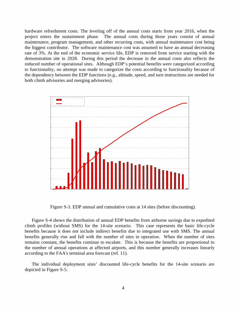
Estimated annual EDP costs in year 2000 dollars (before discounting) for the 14-site case are shown in Figure S-3. The figure shows the initial R&D costs, then increasing implementation costs, then a leveling off, followed by generally decreasing costs with occasional peaks representing

4

hardware refreshment costs. The leveling off of the annual costs starts from year 2016, when the project enters the sustainment phase. The annual costs during those years consist of annual maintenance, program management, and other recurring costs, with annual maintenance cost being the biggest contributor. The software maintenance cost was assumed to have an annual decreasing rate of 3%. At the end of the economic service life, EDP is removed from service starting with the demonstration site in 2028. During this period the decrease in the annual costs also reflects the reduced number of operational sites. Although EDP’s potential benefits were categorized according to functionality, no attempt was made to categorize the costs according to functionality because of the dependency between the EDP functions (e.g., altitude, speed, and turn instructions are needed for both climb advisories and merging advisories).

Figure S-3. EDP annual and cumulative costs at 14 sites (before discounting).

Figure S-4 shows the distribution of annual EDP benefits from airborne savings due to expedited climb profiles (without SMS) for the 14-site scenario. This case represents the basic life-cycle benefits because it does not include indirect benefits due to integrated use with SMS. The annual benefits generally rise and fall with the number of sites in operation. When the number of sites remains constant, the benefits continue to escalate. This is because the benefits are proportional to the number of annual operations at affected airports, and this number generally increases linearly according to the FAA's terminal area forecast (ref. 11).

The individual deployment sites’ discounted life-cycle benefits for the 14-site scenario are depicted in Figure S-5.

$0

$5

$10

$15

$20

$25

$30

$35

$40

$45

2002 2004 2006 2008 2010 2012 2014 2016 2018 2020 2022 2024 2026 2028 2030 2032 2034 2036

Year

An

nu

al C

ost

s (Y

r200

0$M

)

$0

$50

$100

$150

$200

$250

$300

$350

$400

$450

Cu

mu

lati

ve C

ost

s (Y

r200

0$M

)

Annual Costs

Cumulative Costs

5

Figure S-4. EDP-Climb w/o SMS annual and cumulative benefits at 14 sites (before discounting).

Figure S-5. EDP-Climb w/o SMS discounted life-cycle benefits of each site (year 2000 $M).

$0

$15

$30

$45

$60

$75

2002 2004 2006 2008 2010 2012 2014 2016 2018 2020 2022 2024 2026 2028 2030 2032 2034 2036

Year

An

nu

al B

enef

its

(Yr2

000$

M)

$0

$250

$500

$750

$1,000

$1,250

Cu

mu

lati

ve B

enef

its

(Yr2

000$

M)

Annual Benefits (EDP-Climb w/o SMS)

Cumulative Benefits

PCT

A90N90

A80

MIA

D21PIT

M98

C90

D10

I90

x D01NCT

SCT $9.2

$72.7

$67.2

$54.0

$31.7

$15.9

$8.5

$6.2

$5.3

$4.6

$2.5

$2.6$16.4

$4.2

x

x

x

x

x

x

x

x

x

x

xx

x

PCT

A90N90

A80

MIA

D21PIT

M98

C90

D10

I90

x D01NCT

SCT $9.2

$72.7

$67.2

$54.0

$31.7

$15.9

$8.5

$6.2

$5.3

$4.6

$2.5

$2.6$16.4

$4.2

x

x

x

x

x

x

x

x

x

x

xx

x

6

Life-Cycle Cost Contributors

Table S-2 shows the EDP life cycle cost distribution of the identified cost factors (after discounting). The most important cost factors in both the 9-site and 14-site scenarios are software maintenance, FAA program management (including program management/technical support, management personnel, supplies and travel, miscellaneous studies, contract award process, and independent verification and validation costs), and FAA software development (including development, management and administrative services, integrated logistic support, and training development). The highlighted entries in the 14-site column denote a reversal in rank against the 9-site case. This reversal is partly due to the time-value of money (e.g., the software maintenance phase for the 14-site case starts 3 years later than for the 9-site case). The presumed negligible cost associated to the integration with SMS, necessary to the realization of ground savings, is not assessed.

Table S-2. EDP cost factors (Year 2000 $M, discounted).

Cost Factors 9-site 14-site Software Maintenance $29.5 $24.1 FAA Program Management $24.4 $26.3 FAA Software Development $23.7 $26.0 Implementation $11.7 $15.7 Hardware $11.2 $15.8 Systems Engineering $8.5 $10.9 NASA Development Costs $6.5 $6.5 In-Service management $5.0 $5.1 Test and evaluation $4.3 $6.1 In-Service Support $3.5 $4.9 Adaptation $3.0 $4.2 Integration $1.9 $2.7 Configuration Management $1.2 $1.5 Software License $0.8 $1.1 IOT&E $0.6 $0.9

Total $135.6 $151.7

Life-Cycle Cost/Benefit Economic Metrics

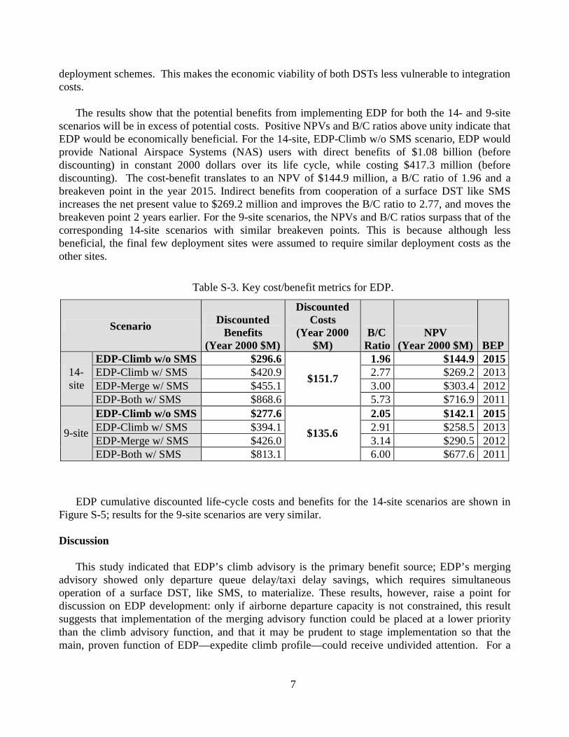
Table S-3 shows the economic metrics, including Net Present Value (NPV), Benefit to Cost ratio (B/C ratio), and Breakeven Point (BEP), for both scenarios. Under either the 14-, or the 9-site deployment scenario, EDP-Climb without SMS, EDP-Climb with SMS, EDP-Merge with SMS, and EDP-Climb&Merge with SMS are evaluated separately. As mentioned in the last paragraph, because we did not estimate EDP’s integration costs with SMS, only one LCC each for the 14- and 9-site scenarios were assessed. Therefore, the LCCBA results for the “with SMS” cases are of relatively low precision. Note that a recent LCCBA of SMS (ref. 31) estimated generally higher potential benefits and B/C ratio for SMS than the values for EDP shown in Table S-3 with similar

7

deployment schemes. This makes the economic viability of both DSTs less vulnerable to integration costs.

The results show that the potential benefits from implementing EDP for both the 14- and 9-site scenarios will be in excess of potential costs. Positive NPVs and B/C ratios above unity indicate that EDP would be economically beneficial. For the 14-site, EDP-Climb w/o SMS scenario, EDP would provide National Airspace Systems (NAS) users with direct benefits of $1.08 billion (before discounting) in constant 2000 dollars over its life cycle, while costing $417.3 million (before discounting). The cost-benefit translates to an NPV of $144.9 million, a B/C ratio of 1.96 and a breakeven point in the year 2015. Indirect benefits from cooperation of a surface DST like SMS increases the net present value to $269.2 million and improves the B/C ratio to 2.77, and moves the breakeven point 2 years earlier. For the 9-site scenarios, the NPVs and B/C ratios surpass that of the corresponding 14-site scenarios with similar breakeven points. This is because although less beneficial, the final few deployment sites were assumed to require similar deployment costs as the other sites.

Table S-3. Key cost/benefit metrics for EDP.

Scenario Discounted

Benefits (Year 2000 $M)

Discounted Costs

(Year 2000 $M)

B/C Ratio

NPV (Year 2000 $M) BEP

EDP-Climb w/o SMS $296.6 1.96 $144.9 2015EDP-Climb w/ SMS $420.9 2.77 $269.2 2013EDP-Merge w/ SMS $455.1 3.00 $303.4 2012

14-site

EDP-Both w/ SMS $868.6

$151.7

5.73 $716.9 2011


9-site


$135.6

6.00 $677.6 2011

EDP cumulative discounted life-cycle costs and benefits for the 14-site scenarios are shown in Figure S-5; results for the 9-site scenarios are very similar.

Discussion

This study indicated that EDP’s climb advisory is the primary benefit source; EDP’s merging advisory showed only departure queue delay/taxi delay savings, which requires simultaneous operation of a surface DST, like SMS, to materialize. These results, however, raise a point for discussion on EDP development: only if airborne departure capacity is not constrained, this result suggests that implementation of the merging advisory function could be placed at a lower priority than the climb advisory function, and that it may be prudent to stage implementation so that the main, proven function of EDP—expedite climb profile—could receive undivided attention. For a

8

definitive conclusion, additional simulations could be run and coupled with other types of studies, such as a Cost as an Independent Variable analysis.

Figure S-6. EDP cumulative discounted life-cycle costs and benefits for the 14-site scenario.

$0

$100

$200

$300

$400

$500

$600

$700

$800

$900

2002 2004 2006 2008 2010 2012 2014 2016 2018 2020 2022 2024 2026 2028 2030 2032 2034 2036

Year

Ben

efit

s&C

ost

s ($

M, D

isco

un

ted

7%

/Yr)

Discounted Cumulative Costs

Discounted Cumulative Benefits (EDP-Climb w/ SMS)

Discounted Cumulative Benefits (EDP-Merge w/ SMS)

Discounted Cumulative Benefits (EDP-Both w/ SMS)

Discounted Cumulative Benefits (EDP-Climb w/o SMS)

9

1. INTRODUCTION

1.1. Background

The Advanced Air Transportation Technologies (AATT) Project is part of the National Aeronautics and Space Administration’s (NASA’s) Airspace Systems Program. Its objective is to develop Decision Support Tools (DSTs) that are computer-based analysis, prediction, and display aids for air traffic controllers. These tools will facilitate substantial increases in the effectiveness of the national air transportation system. The AATT project is responsible for defining, exploring, and developing the DSTs to a level suitable for pre-production prototype assessment by the Federal Aviation Administration (FAA). During the course of the NASA research and development effort, NASA conducts life-cycle cost/benefit studies at several stages of maturity to indicate whether the DST will have a positive return on investment if deployed by the FAA.

One of these DSTs, Expedite Departure Path (EDP), is currently in the technology development phase at NASA Ames Research Center. EDP is aimed at providing Terminal Radar Approach Control (TRACON) Traffic Management Coordinators (TMCs) with appropriate departure traffic demand and scheduling information, and providing departure controllers with advisories for tactical control of TRACON departure traffic. The EDP advisories will assist TRACON departure controllers in efficiently sequencing, spacing and merging departure aircraft into en route traffic streams.

We performed an initial life-cycle cost/benefit assessment (LCCBA) of seven AATT DSTs, including EDP, for NASA in fiscal year 2001 (ref. 1). The estimated life-cycle potential benefits of EDP in reference 1 were based on an earlier potential benefits assessment (ref. 2). This previous EDP potential benefits assessment was based on a methodology that resulted in overly optimistic estimates. This report documents a refined benefits assessment for EDP. The life-cycle cost (LCC) assessment was also updated based on information obtained from the FAA that more accurately captures the FAA’s DST acquisition characteristics (ref. 3). Adjustments were also made to the site selection and deployment scheduling methodology to include airspace complexity as a factor. This technique was also applied to the benefit-extrapolation methodology to estimate potential benefits for other years, and at other sites.

From here on, unless stated otherwise, the terms “cost” and “benefit” in this report refer to “potential cost” and “potential benefit,” respectively.

1.2. Objectives

The primary objective of this report is to provide a refined LCCBA for EDP.

This study is, for the most part, a “non-integrated” assessment, in that it does not generally take into account the differential cost and benefit of having other DSTs already functioning at a site. However, for some EDP functionality, it was very easy to also assess the EDP benefits that would occur if EDP were integrated with a departure planning and managing system like Surface Management System (SMS). These incremental EDP benefits (indirect benefits) are also provided

10

in the report, and are the exception to the “non-integrated” assessment. However, the costs associated with the DSTs’ integration effort are not estimated. Thus, whenever possible, the LCCBA study without the influence of SMS is used as the illustrative example; the “w/SMS” LCCBA results should be viewed with this in mind.

1.3. Previous Work

There have been three previous studies of EDP benefits (refs. 2, 4, and 5).

A 1998 study (ref. 4) reported two EDP benefit mechanisms: 1) providing suggested clearances to controllers that balance flows to departure fixes; and 2) pointing out to controllers opportunities for efficient climb-out paths during simultaneous arrival and departure operations. The benefits assessment methodology included analysis of times-to-climb for departures from busy and less-busy airports, and then assessed corresponding EDP benefits as a reduction of daily average times-to-climb at busy airports to values characteristic of less-busy airports. The study predicted a mean reduction in departure time spent in the TRACON of 3 minutes. This resulted in a $232 million (1996 $) annually at 16 airports for the year 2005 according to reference 4. This approach was suitable at that time, because the EDP functionality was not fully defined during the basic technology research phase.

A 1999 study (ref. 5) reported five EDP benefit mechanisms:

• Provide sequencing and spacing advisories that enable reduced spacing buffers,

• Improve runway system utilization by coordinating sequencing and spacing action between arrival and departure traffic,

• Expedite climbs with user-preferred speed and departure profiles due to improved trajectory control,

• Coordinate scheduling of gate departures, takeoff, and departure fix crossing to reduce ground and airspace delay, and

• Facilitate efficient merging of departures from satellite airports with traffic streams of major airports.

The benefit assessment methodology of reference 5 involved determining the sensitivity of EDP and supporting technologies to various trajectory accuracy parameters and evaluating the resulting, enhanced capability of the Air Traffic Management (ATM) system to predict and control trajectories. The improved prediction and control resulted in decreased total delay, changes in delay distribution, and improved flight schedules and trajectories. Assessment was performed using a computer-based simulation model, and showed delay savings of 6 minutes per IFR departure; 1 minute per IFR arrival; 1 minute per VFR departure; and 2 minutes per VFR arrival. These savings translated into $278 million (1996 $) annually at 10 airports for the year 1996, and $2.47 billion (1996 $) annually at 43 airports for the year 2015.

11

A 2001 study (ref. 2) reported 17 EDP benefit mechanisms, and quantitatively assessed only the three primary benefit mechanisms: reduction of climb-out time due to unrestricted climb, optimal merging of departures due to tactical speed and heading advisories, and reduction of taxi-out delay due to EDP advisories interfacing with ground DSTs. The study used Enhanced Traffic Management System (ETMS) data to generate a baseline demand, and assessed EDP benefits as applying to all restricted climbs, which were flights that were delayed in reaching cruise altitude, flights that were cleared to a lower than optimal altitude, and flights that filed for a lower than optimal altitude. Stand-alone EDP benefits were assessed in terms of reduced climb-out times and fuel burn. Taxi-out delay benefits, which would require presence of another DST, were analyzed using Consolidated Operations and Delay Analysis System (CODAS) data in comparison to airport capacity data. In 1999, individual aircraft delays ranged from roughly 0 to 2 minutes during the climb-out phase, and from 0 to 9 minutes during taxi-out. The collective, potential EDP benefits at ten deployment sites, within the system of 42 airports considered, was assessed to be $921 million (1997 $) for 1999 ($189 million without ground delay savings) and $1.15 billion (1997 $) for 2015. The direct EDP potential benefits (without those due to taxi-out delay savings) for the 2015 time frame was not given.

Among the three reports, reference 2 is the most recent and detailed. However, it provided only the upper bound of potential benefits achievable by EDP. It was also the only study that considered ground-delay savings. The single year EDP benefit estimated in this study was used in the previous LCCBA of EDP (ref. 1). This LCCBA used ten deployment sites, and is now believed to be inaccurate with inflated benefits and underestimated costs, yielding a NPV of $859 million (year 2000$), and benefit to cost ratio of 21.

The progress in EDP development and additional cost information on similar DSTs promote a refined LCCBA study of EDP.

1.4. Report Organization

Functionality of EDP is described briefly in Section 2, which also includes a discussion of EDP’s operational concept, benefit mechanisms, and benefit metrics. Section 3 presents the LCCBA methodology used in this study. Section 4 provides EDP simulation methods and benefits results. This is followed by a section with a brief account of cost analysis. Section 6 presents EDP LCCBA assessment results and discusses those results. Unless otherwise noted, all monetary results are expressed in year 2000 dollars. A summary is provided in Section 7, which concludes this report.

12

2. EDP FUNCTIONALITY AND BENEFIT MECHANISMS

The goal of EDP is to provide assistance that enhances the controllers’ ability to efficiently direct traffic into en route streams. EDP is designed to provide departure controllers with optimized schedules and advisories, while meeting constraints from flow control and ensuring the efficient and safe flow of outbound traffic from airports into en route control sectors. Specifically, EDP will provide departure controllers with climb profile and lateral path guidance advisories to facilitate efficient, uninterrupted climb-out, and safe merging of aircraft into en route traffic.

2.1. Operational Concept

A significant portion of the following description has been taken directly from various EDP documents (ref. 6-9).

EDP is currently in the technology development phase. Some concept development work, initial human-factors studies, and preliminary potential benefits studies have been completed. A few controller-in-the-loop simulations have also been conducted at the time that this report was written. The functions and benefits listed in this report are based on the envisioned full functionality of EDP and are described in the future tense.

EDP will be a terminal area DST for assisting controllers in managing airborne departure traffic in congested terminal airspace. EDP will also assist the controller in expediting conflict-free trajectories to aircraft equipped with automatic, 4-D tracking capability (data-linked FMS). The purposes of EDP are to:

• Increase the efficiency of departure operations while maintaining or increasing current levels of safety,

• Facilitate reductions in fuel burn, noise impact, and terminal area emissions with respect to current departure-traffic management practices,

• Provide accurate pre-departure time-to-fly estimates to ground-based departure planning tools that will result in reduced departure queue delay/taxi delays because of their combined, enhanced ability to match airspace throughput to capacity.

The EDP network (see Figure 2-1) uses aircraft flight plans and position data from FAA computers, inputs from TRACON departure controllers, and current weather predictions to produce advisories that assist controllers in managing departure traffic. TRACON departure controllers interact with EDP, both receiving advisories and providing inputs through standard FAA hardware. EDP will provide departure controllers with timely textual and graphical advisories for efficient control of airborne departure aircraft. Heading, speed, and altitude advisories will be presented in a tactical manner, to be issued by the controller as control directives to the flight deck. The EDP human interface may include a mean for the controller to provide feedback by indicating to the system when he/she has issued an advised control instruction to the aircraft. Since this would improve the trajectory prediction accuracy of EDP and therefore increase its efficiency benefits, the

13

EDP developers would like to include this feature, however its presence will depend on whether controllers would accept and use this interface. Center TMCs receive strategic information and input facility operational data (e.g., airspace configuration, surface conditions, inter-facility miles-in-trail constraints, etc.), but do not provide feedback to EDP. Both Center and TRACON TMCs receive information from EDP through a dedicated display.

Figure 2-1. EDP system overview.

EDP will be part of the CTAS tool suite; it will share the 4-D trajectory prediction software module based on aircraft performance models with Traffic Management Advisor (TMA) and Descent Advisor (DA). Trajectory profile selection and clearance advisories developed for Final Approach Spacing Tool (FAST) will be employed in EDP’s TRACON-tool component. EDP will employ conflict prediction technology developed for the DA and Direct-to DSTs, as well as a knowledge-based conflict resolution scheme shared by active Final Approach Spacing Tool (aFAST).

14

2.2. Functionality

The following functionality has been proposed for EDP:

• Climb Advisories: EDP will utilize conflict probe functionality to expedite departures that cross arrival routes by determining when unrestricted climbs can be given to specified aircraft (in TRACON airspace).

• Merging Advisories: EDP will provide metering and/or clearance advisories for departing aircraft that will merge with en route traffic over a given fix. The merging advisories lead to precise spacing over departure fixes or departure gates that deliver aircraft along conflict-free trajectories into en route traffic streams. This type of advisory may be replaced by direct route advisories in the future (see below).

• Tactical Advisories: EDP will provide conflict-free, fuel-efficient speed and turn advisories to improve utilization of terminal airspace and provide precision trajectory tracking.

• Accurate Time-to-fly Estimates: EDP will provide accurate flying time estimates to surface-based departure planning systems. This allows airborne delays to be transferred to the departure queue on the ground, and is manifested as improved departure sequencing.

• Direct Route Advisories: This function is a future EDP capability. EDP will provide advisories that will support direct route transition to en route flight by eliminating routing restrictions.

2.3. Benefit Mechanisms and Metrics

The various EDP functions previously described give rise to specific benefit mechanisms that can be measured by appropriate benefit metrics. These are discussed for each EDP function.

2.3.1. Climb Advisories

Many major TRACONs procedurally restrict departure paths below arrival paths. This restriction is often made when there is an intersection between an arrival route and a departure route close to the airport. In these cases, controllers restrict the departing aircraft to an altitude below the incoming arrival stream until the controller is sure that there is no chance for a conflict. There is a tendency for controllers to restrict departures in order to ensure separation even when separation is otherwise assured by the 4-dimensional geometry of a situation (see Figure 2-2). This conservative procedure is called “tunneling.” Tunneling interrupts optimal climb profiles.

By providing tactical advisories for control of departure aircraft, EDP is able to accurately predict their future position. With the knowledge of aircraft flight plans and arrival procedures, EDP is also able to accurately predict future positions of arrival and en route aircraft. With accurate positional information of both arrivals and departures, EDP is able to identify opportunities to safely advise expedited climbs for some aircraft (see Figure 2-2), thereby removing the procedural restriction of tunneling.

15

Expedition of climb is a benefit mechanism that facilitates reductions in flight time, fuel burn, departure queue delay/taxi delay1, arrival delay (for dual use runways), noise impact and near-ground emissions. The effect of climb advisories is summarized in Figure 2-3.

Figure 2-2. Climb advisories from EDP.

Figure 2-3. Benefit mechanisms and metrics due to climb advisories with EDP.

2.3.2. Merging Advisories

Merging over a Fix Under current operating conditions, it is often the case that different departure controllers are

working separate aircraft bound for the same fix. To accommodate this situation, controllers are required to space their departures using miles-in-trail constraints, which creates gaps in the streams of aircraft to allow for potential merges. Often, no attempt is made to sequence or space the traffic

1 Although both are delays on the ground, departure queue delay is incurred only when an aircraft is waiting in the departure queue. However, it is hard to distinguish between the two sometimes. This study treats departure queue delay and taxi delay the same and assumes they are possible potential benefits when EDP and SMS operate together.

< 250 kts

Current: Unnecessarily restrict departureaircraft under arrival (“tunneling”). With EDP: Unrestricted climbs.

Climb advisories Expedited climb profiles

Reduced flight time

Reduced fuel burn



Reduced emission

Reduced noise impact

Climb advisories Expedited climb profiles

Reduced flight time

Reduced fuel burn



Reduced emission


16

on an aircraft-by-aircraft basis. This can create situations where one departure stream is empty while another is unnecessarily constrained (see Figure 2-4).

Even if there are no unnecessary constraints, there are cases when aircraft directed by multiple departure controllers would arrive over a fix at the same time (see Figure 2-5). This causes additional workload on the controller trying to sequence and space the aircraft beyond the fix, which often leads to placement of additional miles-in-trail constraints.

EDP merging advisories are designed to reduce these inefficiencies and create precision spacing. EDP calculates and compares the trajectories for each departing aircraft bound for a fix. With EDP’s speed and heading advisories, aircraft can ensure crossing the fix in the correct sequence and with the appropriate spacing. EDP’s algorithms generate a precision 4-D schedule that sequences and spaces the traffic within a quantifiable tolerance of the desired spacing (see Figure 2-4 and Figure 2-5).

Figure 2-4. Merging over a fix with EDP – removes unnecessary constraints.

Figure 2-5. Merging over a fix with EDP – reduces inefficient sequencing.

Excess Spacing

Current: One departure route empty, while the otheris unnecessarily constrained.

With EDP: Spaces the traffic as close to the desiredresult as feasible.

Current: Sequencing and spacing required beyond the fix often lead to additional miles-in-trail constraints.

With EDP: Speed and vector advisories allow for departure aircraft to be sequenced and spaced laterally

for a smooth transition into the en route system.

Different altit

udes

Different altit

udes

Current: Sequencing and spacing required beyond the fix often lead to additional miles-in-trail constraints.

With EDP: Speed and vector advisories allow for departure aircraft to be sequenced and spaced laterally

for a smooth transition into the en route system.

Different altit

udes

Different altit

udes

17

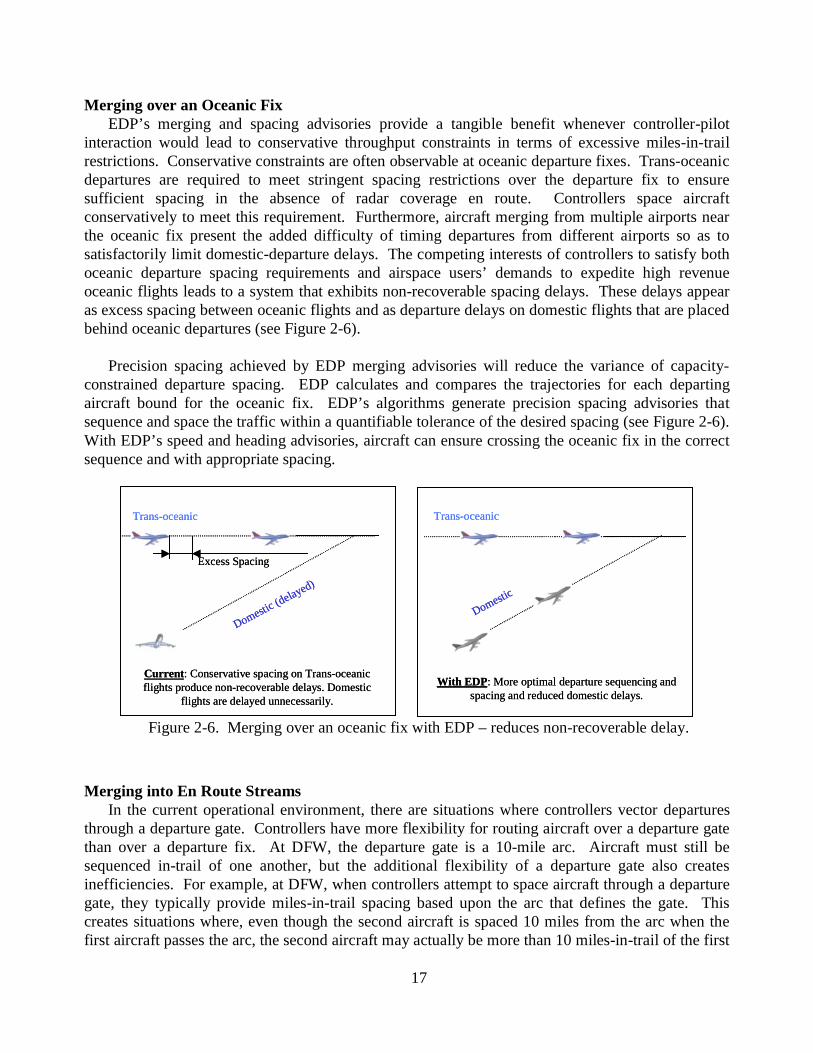
Merging over an Oceanic Fix EDP’s merging and spacing advisories provide a tangible benefit whenever controller-pilot

interaction would lead to conservative throughput constraints in terms of excessive miles-in-trail restrictions. Conservative constraints are often observable at oceanic departure fixes. Trans-oceanic departures are required to meet stringent spacing restrictions over the departure fix to ensure sufficient spacing in the absence of radar coverage en route. Controllers space aircraft conservatively to meet this requirement. Furthermore, aircraft merging from multiple airports near the oceanic fix present the added difficulty of timing departures from different airports so as to satisfactorily limit domestic-departure delays. The competing interests of controllers to satisfy both oceanic departure spacing requirements and airspace users’ demands to expedite high revenue oceanic flights leads to a system that exhibits non-recoverable spacing delays. These delays appear as excess spacing between oceanic flights and as departure delays on domestic flights that are placed behind oceanic departures (see Figure 2-6).

Precision spacing achieved by EDP merging advisories will reduce the variance of capacity-constrained departure spacing. EDP calculates and compares the trajectories for each departing aircraft bound for the oceanic fix. EDP’s algorithms generate precision spacing advisories that sequence and space the traffic within a quantifiable tolerance of the desired spacing (see Figure 2-6). With EDP’s speed and heading advisories, aircraft can ensure crossing the oceanic fix in the correct sequence and with appropriate spacing.

Figure 2-6. Merging over an oceanic fix with EDP – reduces non-recoverable delay.

Merging into En Route Streams

In the current operational environment, there are situations where controllers vector departures through a departure gate. Controllers have more flexibility for routing aircraft over a departure gate than over a departure fix. At DFW, the departure gate is a 10-mile arc. Aircraft must still be sequenced in-trail of one another, but the additional flexibility of a departure gate also creates inefficiencies. For example, at DFW, when controllers attempt to space aircraft through a departure gate, they typically provide miles-in-trail spacing based upon the arc that defines the gate. This creates situations where, even though the second aircraft is spaced 10 miles from the arc when the first aircraft passes the arc, the second aircraft may actually be more than 10 miles-in-trail of the first

Current: Conservative spacing on Trans-oceanic flights produce non-recoverable delays. Domestic

flights are delayed unnecessarily.

Excess Spacing

With EDP: More optimal departure sequencing and spacing and reduced domestic delays.

Trans-oceanicTrans-oceanic

Domestic

Domestic (d

elayed)

Current: Conservative spacing on Trans-oceanic flights produce non-recoverable delays. Domestic

flights are delayed unnecessarily.

Excess Spacing

With EDP: More optimal departure sequencing and spacing and reduced domestic delays.

Trans-oceanicTrans-oceanic

Domestic

Domestic (d

elayed)

18

aircraft based on a direct measurement (see Figure 2-7). Precision merging advisories provided by EDP will enable more efficient spacing procedures. The precise calculations of EDP advisories can also reduce the number of clearances required to achieve the desired spacing or sequencing.

Figure 2-7. Merging over a departure gate with EDP – reduces inefficient spacing.

Precision spacing performed with EDP is a benefit mechanism that facilitates reductions in flight time, fuel burn, departure queue delay/taxi delay, arrival delay for dual use runways, and emissions. The beneficial effects of merging advisories that facilitate precision spacing for merges either over a fix, or a departure gate, are summarized in Figure 2-8.

Figure 2-8. Benefit mechanisms and metrics due to merging advisories with EDP.

2.3.3. Tactical Advisories

EDP’s tactical speed and heading advisories facilitate precision tracking of prescribed trajectories that are conflict-free and meet schedule, fuel efficiency, and/or noise mitigation objectives. These advisories also enable EDP to meet merging constraints.

Benefits associated with meeting scheduling and fuel efficiency objectives are manifested in precision spacing and expedited climb benefit mechanisms. EDP can proactively minimize

Current: Even though the second aircraft is spaced 10 miles away from the gate (arc), it may be > 10 miles

away from the first aircraft.

Departure Gate (sometimes a 10

mile arc)10 mi

> 10 mi


mile arc)

With EDP: Aircraft are spaced from the aircraft that they will follow after merging instead of from the arc.

10 mi

Current: Even though the second aircraft is spaced 10 miles away from the gate (arc), it may be > 10 miles

away from the first aircraft.


mile arc)10 mi

> 10 mi


mile arc)

With EDP: Aircraft are spaced from the aircraft that they will follow after merging instead of from the arc.

10 mi


Reduced flight time

Reduced fuel burn



Reduced emission


Reduced flight time

Reduced fuel burn



Reduced emission

19

community noise impact and reduce cost of environmental impact studies. EDP would issue tactical advisories, based on the noise optimal path it calculated, to insure that aircraft follow this path precisely. Noise mitigating profiles generally do not have direct operating cost associated with them, but they do affect the cost of community improvements falling within the noise-footprint of an airport. While emissions are not currently measured, tracked, or penalized in the same manner as noise, it is conceiveable that future systems will attempt to do just that. Precision trajectory tracking, which is enabled by EDP’s tactical advisories is, therefore, a benefit mechanism for reduced noise and emission impact. This relationship is summarized in Figure 2-9.

Figure 2-9. Benefit mechanisms and metrics due to tactical advisories with EDP.

2.3.4. Accurate Time-to-fly Estimates

EDP’s trajectory estimates are of much higher quality than those provided by departure sequencing tools currently in use. EDP produces high quality predictions of when aircraft will reach departure fixes or gates. These accurate, departure time-to-fly estimates can be used by departure sequencing tools in forming departure sequences that will optimize the airport throughput. The improved departure sequence reduces airborne delay and accurately propagates delay back to the departure queue on the ground. Thus, the improved departure sequencing benefit mechanism leads to reduced airborne departure delay, reduced arrival delay on dual use runways, reduced departure queue delay/taxi delays (will also result in reduced fuel burn costs), and reduced emissions (see Figure 2-10).

Figure 2-10. Benefit mechanisms and metrics due to accurate time-to-fly estimates of EDP.

2.3.5. Direct Route Advisories

Direct en route transition is anticipated as a future EDP capability. Flexibility offered by elimination of routing restrictions with EDP’s direct route advisories will increase the potential value of wind-optimal routes to the airspace user. Eliminating routing restrictions is a benefit mechanism for reduced flight time, reduced fuel burn, reduced departure queue delay/taxi delay,





Reduced emission

Reduced fuel burn





Reduced emission

Reduced fuel burn

Tactical advisoriesPrecision trajectorytracking

Reduced emission


20

reduced arrival delay on dual use runways, reduced emissions, and reduced noise impact (see Figure 2-11).

Figure 2-11. Benefit mechanisms and metrics due to direct route advisories with EDP.

Direct route advisoriesEliminate routing restrictions

Reduced flight time

Reduced fuel burn


Reduced arrival delay (for dual use runway)

Reduced emission


Direct route advisoriesEliminate routing restrictions

Reduced flight time

Reduced fuel burn


Reduced arrival delay (for dual use runway)

Reduced emission


21

3. LIFE-CYCLE COST/BENEFIT ASSESSMENT METHODOLOGY

3.1. Methodology Overview

The LCCBA methodology used in this report, and summarized in Figure 3-1, is derived from a previous LCCBA of seven AATT DSTs performed in 2001 (ref. 1). The methodology includes site selection analysis, site deployment schedule development, cost and benefit assessment models, and is followed by the life-cycle cost/benefit assessment. The site selection analysis provides a prioritized list of deployment sites for EDP. A site schedule was developed for EDP deployment using this ordered list and the site deployment scheduling methodology. Given the schedule of deployment at the various sites, EDP annual costs and benefits were assessed. The costs and benefits were combined in a life-cycle cost/benefit analysis.

Figure 3-1. Overview of life-cycle cost-benefit assessment methodology.

3.2. Site Selection

NASA’s EDP developers identified the following 14 sites (TRACONs) as possible future EDP deployment sites: Southern California (SCT), New York (N90), Potomac (PCT), Northern California (NCT), Chicago (C90), Atlanta (A80), Dallas Ft. Worth (D10), Denver (D01), Houston (I90), Boston (A90), Detroit (D21), Miami (MIA), Minneapolis (M98), and Pittsburgh (PIT). The developers predicted that there would be three groups (banks) of deployment sites. To reflect this, these sites were sorted into three groups according to likelihood of generating potential EDP benefits. NASA EDP engineers and the authors agreed that complexity of and volume of operations in the TRACON airspace are key factors in determining deployment priority.

In an earlier exploration of methodology to categorize NAS deployment of AATT DSTs (ref. 10), we identified the number of departure stream merges together with the total number of operations as measures of the potential benefit of EDP at a site. The first parameter was approximated by the number of possible pairings of “EDP-affected” airports that could be selected

Site Selection

SiteDeployment

Schedule

BenefitAssessment

CostAssessment

Life-CycleCost/Benefit

Site deployment order

22

from the collection of airports within a TRACON, i.e., C(n,2)2. This approximation is based on the assumption that there are roughly equal interactions between each pair of airports. It was then assumed that potential EDP benefits at a TRACON are directly proportional to the product of C(n,2) and the total number of operations at that site.

We modified that methodology for this study by using a slightly different representation of airspace complexity. Rather than deriving the airspace complexity parameter from the combination number of all airports, the number of “uncoordinated” departure runways of neighboring airports within the TRACON for a given airport “ i ,” im was used. An “uncoordinated” runway is defined from the perspective of a specific airport as a departure-only or a mixed-use runway at another airport within its surrounding TRACON. Despite its simplicity, we believe that the number of “uncoordinated” departure runways within a TRACON is a key indicator of the potential for EDP to produce benefits for a given airport. In summary, the following steps were taken to determine the order of site deployment:

• Calculate the total number of “uncoordinated” departure runways for “EDP-affected” airport “ i ,” im .

• Determine the number of “EDP-affected” operations for that airport, iEDPn , .

• After multiplying the above two factors for each airport at the site, sum the products to yield a value signifying the Relative Potential Benefits (RPB) of EDP.

∑ ×=i iiEDPEDP mnRPB )( ,

The above procedure is very straightforward excepting the following two issues: how to determine which airports at a site are “EDP-affected,” and what constitutes an “EDP-affected” operation (will be referred simply as “EDP” operations hereon). These issues are briefly addressed below.

For this assessment, we decided to use the NASA-provided set of 42 airports in the NAS as the “primary” “EDP-affected” airports3 (see Table 3-1). However, a “screen” was needed so that we could include consideration for other airports that would have a sizeable impact on the potential benefit of EDP. These will be referred to as “secondary” “EDP-affected” airports. Ideally, all flights that share the use of the busiest airspace (mostly jets) within the terminal area where EDP is designed to provide benefits would be included. Operations in this airspace are typically air carrier and air taxi. Special consideration will be given to airports with a large number of jet operations, even if the number of air carrier and air taxi operations is small. In other words, this assessment assumes all jet-engine aircraft operations at an “EDP-affected” airport as “EDP” operations.

2 Read this as “the possible number of unique combinations of two items, taken from a set of n unique items; with replacement.” C(n,2) = [n × (n-1)] / 2.

3 The only exception is Long Beach (LGB) in Southern California TRACON. The reason will be explained shortly.

23

Table 3-1. Potential EDP deployment sites – primary airport information (ref. 10).

Nominal Flow – Runway Used Site ID

Airport ID

Nominal Traffic Flow Arrival Departure Mixed

2000 Total

Operations

LAX West Flow (>90%) 24R, 25L 24L, 25R 781,418SCT

SAN West Flow 27 208,894EWR SW Flow 22L 22R 11 458,677JFK SE Flow 13R 13L 358,977LGA South Flow 22 13 378,018HPN N/S (50% Each) 16/34 217,939

N90

TEB South Flow 19 24 270,301IAD North Flow 01R 30 01L 495,717DCA North Flow 33 03, 01 344,092PCT BWI West Flow 33L 28 33R 309,516SFO West Flow 01R, 01L 28R, 28L 437,763

NCT OAK West Flow 29 478,558ORD East Flow 04R, 09R 04L, 32L 09L 906,326

C90 MDW NW Flow 31C 301,879

A80 ATL West Flow (63%) 26R, 27L 26L, 27R 922,016

D10 DFW South Flow (>70%) 13R, 18R, 17C, 17L

13L, 18L, 17R

875,673

D01 DEN South Flow 16, 26 17R 520,882IAH West Flow 27 14L 26 483,806

I90 HOU West Flow 30L 22 254,900

A90 BOS South Flow 15R 22L, 22R 510,113D21 DTW South Flow 21R 21L 21C 561,123

MIA East Flow 09R, 12 09L 516,009MIA

FLL East Flow 09L 287,094M98 MSP North Flow (51%) 30L, 30R 524,261PIT PIT West Flow 28L, 28R 28C 449,168

Thus, for most “primary” airports, where General Aviation (GA) flights are sparse, all operations are assumed to be “EDP” operations. Arrival operations are included to account for possible benefits on arrivals. These operation numbers were obtained from the FAA’s Terminal Area Forecast website (ref. 11). For the “secondary” airports, the larger of the air carrier/air taxi operations (ref. 11) and the deduced number of jet operations was used as the number of “EDP” operations. It was further assumed that the percentage of jet operations at an airport is proportional to the percentage of jet aircraft based at the airport which is available from reference 12.

During the site visit to the Potomac TRACON, we were told that the operations at Andrews Air Force Base (ADW) would be important to the simulation of traffic of the Washington metro area, but its contribution to the potential benefits of EDP would be marginal. Furthermore, the operations at ADW are primarily jets. Thus, we decided to construct a filter to remove airports that would have less impact than ADW from consideration. The ratio of projected departure operations at ADW to

24

the projected total of departure operations from the primary airports of the Potomac TRACON (IAD, BWI, and DCA) was the lower bound. This ratio is referred to as TRACON Operations Ratio or TOR. As calculated from the TAAM simulation model obtained from the FAA, the lower bound of TOR is roughly 6.5%. This filter excludes airports with primarily general aviation operations such as Love Field airport near DFW (TOR of 0.5% for the year 2000). This filter also identifies Long Beach airport (LGB) in the Southern California TRACON as a special case among the 42 NASA-provided airports: its TOR is projected to be 2.0% as calculated for the year 2000, and is not included in this assessment. A second filter was constructed and used to exclude airports that are far away from the “primary” airport(s). In such cases, these airports do not have significant interaction with other traffic within the TRACON. A representative case is the Sacramento area airports in Northern California TRACON4. For non-primary airports that passed the “screens,” it was assumed that they each have one runway used for departure. These “secondary” airports are listed in Table 3-2, along with their number of “EDP” operations (arrivals plus departures) for year 2000.

Table 3-2. Potential EDP deployment sites – secondary airport information.

Site ID

Airport ID

Departure Runways (assumed)

2000 “EDP” Operations

2000 TOR

BUR 1 88,310 8.9%ONT 1 122,301 12.4%SNA 1 99,266 10.0%

SCT

VNY 1 87,901 8.9%N90 - - -PCT ADW 1 69,773 6.5%NCT SJC 1 156,620 17.1%C90 - - -A80 - - -D10 - - -

D01 APA 1 45,427 8.7%I90 EFD 1 48,592 6.6%A90 - - -D21 - - -MIA - - -M98 - - -PIT - - -

Using the above information, the RPB for each site is calculated and plotted in Figure 3-2. As can be seen, a rough grouping of 4, 5, and 5 sites can be identified. Thus, the first bank of deployment sites was chosen to be N90, SCT, PCT, and NCT, with the second bank being C90,

4 Although San Diego airport (SAN) is far away from the number one airport in Southern California TRACON—Los Angeles (LAX), there is enough traffic between them to make SAN important to be included in the assessment of EDP. These flights are sometimes called “TRACON en route” flights.

25

A80, D10, I90, and MIA, and the third bank being D01, D21, A90, PIT, and M98. However, since D10 (DFW) is assumed to be the NASA demonstration site, it was moved up to be the first deployment site. The RPBs from each site for the year 2000 were collected, and normalized to that of PCT and listed in Table 3-3.

Figure 3-2. Ordering of EDP Relative Potential Benefits ranking.

Table 3-3. Normalized EDP Relative Potential Benefits (RPB) for the year 2000.

Site ID RPB

N90 1.29SCT 1.22PCT 1.00NCT 0.66I90 0.30C90 0.29A80 0.15D10 0.14MIA 0.13D01 0.09D21 0.09M98 0.09A90 0.08

PIT 0.07

N90 SCT PCT NCT I90 C90 A80 D10 MIA D01 D21 M98 A90 PIT

Rel

ativ

e P

ote

nti

al B

enef

its

Bank 1Bank 2Bank 3


Rel

ativ

e P

ote

nti

al B

enef

its

Bank 1Bank 2Bank 3

26

A partial deployment scenario involving only the first 2 banks of 9 sites will be studied along with the full 14-site scenario. The TRACONs excluded in the 9-site case are: Denver (D01), Detroit (D21), Minneapolis (M98), Boston (A90), and Pittsburgh (PIT).

3.3. Site Deployment Schedule

A previously developed site deployment scheduling methodology (ref. 1 and 13) was used in this report. In general, the deployment schedules were based on the patterns observed during Free Flight Phase 1 deployment of TMA. The milestones used in the resulting schedule include: Technology Readiness Level (TRL), Initial Daily Use (IDU), Planned Capability Available (PCA), and Installation. The schedule assumptions are summarized below:

• Time between TRL 6 completion to IDU at the 1st site: 0.5 years

• Time between IDU and PCA at a site: 0.5 years

• Time between Installation and IDU at a site: 1.0 years

• Time between Installation of the 1st site and 2nd site: 1.5 years

• Time between Installations of the rest of sites: 0.5 years

• Time between Installation at the last site of a group and the first site of the next group:1.0 years

According to NASA, EDP is currently at TRL 4, and expected to reach TRL 4 completion at the end of this fiscal year (end of 9/2003). Based on experience with Multi-Center TMA (McTMA), the time interval between TRL 4 completion and TRL 6 completion is assumed to be three-and-a-half years.

3.4. Cost Assessment

The life cycle cost (LCC) estimation methodology of reference 14 was used in this report. LCCs are the sums of every cost incurred for a particular system over its lifetime, excepting sunk costs5. LCCs usually include R&D, fabrication and testing, operation, maintenance, and disposal costs. The LCC methodology of reference 14 addressed the three key cost characteristics: (1) consideration of all cost types (coverage); (2) quantification of these costs (estimation); and (3) establishment of temporal schedules to incur these costs (LCC phase). The cost assessment model used a combination of parametric, analogy, and expert opinion techniques, where the parametric technique was used to estimate software related costs. Using Free Flight Phase 1 (FFP1) and Free Flight Phase 2 (FFP2) cost information for Single Center Traffic Management Advisor (TMA or TMA-SC), the cost assessment model was updated and calibrated to reflect actual FAA DST deployment costs (ref.

5 Sunk costs are costs already incurred. The resources represented by these costs have already been consumed and cannot be recovered. According to OMB Circular A-94 (ref. 19), sunk costs shall not be included in the life cycle cost.

27

13). The calibrated cost assessment model of reference 13, with EDP-appropriate input parameters, is used to assess the life cycle costs of EDP in this report.

3.5. Benefit Assessment

3.5.1. Functions, Benefit Mechanisms and Metrics Chosen to be Studied

NASA’s EDP developers suggested that the largest benefits would be derived from climb and merge advisories. In consultation with EDP developers and the NASA technical monitor, it was decided not to examine noise and emission impacts. By not examining noise and emission impacts, some benefits of EDP’s tactical advisories were excluded from this study. It was also decided not to examine the benefits due to direct route advisories because this EDP function is a potential future enhancement to EDP.

As a result of these decisions, only EDP’s climb advisories, merging advisories and accurate time-to-fly estimates were chosen as the basis for quantified, potential benefits. These EDP functions lead to the benefit mechanisms of expedited climb profiles, precision spacing, and improved departure sequencing. EDP benefits will only be measured in terms of reduced flight time, reduced fuel burn, reduced departure queue delay/taxi delay, and reduced arrival delay (for dual use runways). This is summarized in Figure 3-3.

Figure 3-3. Functions, benefit mechanisms and metrics of EDP studied in this report.

Assessing potential EDP benefits from reduction of arrival delay for dual use runways poses additional problems. It is believed that EDP could only help for arrival delays caused by the departure aircraft. Furthermore, EDP would not issue any advisories to arriving aircraft. The simulation software used for this study does not have explicit ways to vary treatment of delays caused by different reasons. It is then assumed in this report that arrivals would not be affected greatly from the use of EDP. However, this assumption may be conservative because a recent study of another DST in the NASA Center/TRACON Automation System (CTAS) tool suite, passive Final Approach Spacing Tool (pFAST), produced savings on departing flights although it focuses on arrival aircraft during final approach.


Reduced fuel burn







Reduced fuel burn






28

3.5.2. Benefit Assessment Methodology

In Section 1.3, methodologies used in previous attempts to assess potential benefits of EDP were briefly described. Although each method has its own advantages, all methodologies had major drawbacks and resulted in optimistic “upper bound” benefits estimates.

The methodology used in reference 4 was developed very early in the effort to define EDP. As a result, it considered only benefits from expedited climb profiles, and was only suitable until additional benefit mechanisms were defined. It also did not account for the operational differences between locations; rather, it assumed that all busy airports will behave like less-busy airports.

Reference 5 attempted to evaluate effects of EDP enabling technologies on the ATM system. This work considered improved capability to predict and control trajectories, and used a dedicated computer simulation approach to determine the sensitivity of various trajectory accuracy parameters of EDP and other decision support tools. However, this work did not consider operational issues and real traffic flows at and around the studied airports.

The most recent assessment of EDP potential benefits was performed in reference 2, and provided an upper bound for potential dollar savings as intended, but used unsatisfactory assumptions. Principal faults were the assumption that “implementation of EDP could eliminate the described delays in the system entirely,” failure to distinguish between causes of delays, and a failure to estimate the effectiveness of EDP under the anticipated range of operational circumstances. For example, we learned from our site visit to Washington DC area FAA air traffic control facilities that, if an aircraft did not fly its optimal cruise altitude due to upper airspace congestion (either because it filed a lower altitude or was delayed at a lower altitude), there is very little chance that a DST like EDP would provide direct improvement. Although reference 2 is believed to provide the most accurate assessment of EDP to date, and includes the most detail6, the methodology needed improvement.

We chose to adopt a fast-time air traffic simulation approach for the benefit assessment of EDP in order to overcome the lack of detail seen in previous studies. It has been shown that fast-time air traffic simulation is a valid approach in air traffic control studies. The particular tool chosen will address the operational issues and traffic flow at and around the study site, including detail that was lacking in previous benefit assessments of EDP. The next section briefly describes the software tool used for the simulation.

Software Selection This study required the use of a software package that simulates air traffic within various ATM

situations, and that provides analysis and visualization tools that can be used to verify simulation results. The software package chosen was the Total Airspace and Airport Modeller (TAAM), a commercial product developed by Preston Aviation Solutions, a wholly owned subsidiary of the Boeing Company. TAAM allows one to go from a qualitative analysis to a quantitative assessment.

6 Reference 2 is the only study that considered ground delay savings.

29

TAAM was also readily available to the authors, and so the model was developed in, and the simulation results were obtained from TAAM Plus, Version 1.1.2 (ref. 15).

TAAM is generally used for fast-time simulations of airport and airspace operations. A TAAM simulation consists of a collection of user-provided data that describe four-dimensional air-traffic scenarios and fulfill all other modeling requirements of the simulation tool. The airport and the airspace environment are built from geographical data, waypoints, airports, routes, sectors, and terrain in the interactive data input system of TAAM. Maps and airport layouts are built using the graphics tool set of TAAM. The factors regulating and limiting air traffic are drawn from a rule-base that includes separation and wake-turbulence spacing criteria, conflict detection and resolution rules, and sequencing decision parameters. The input data are passed to the simulation program where they are processed by TAAM algorithms. Once the TAAM simulation has been successfully started, graphics windows and panels are created. TAAM simulates the air traffic in the environment using an air traffic schedule, aircraft trajectory, and performance-characteristics files. During a simulation, statistics are gathered by a reporting module of TAAM and are written to a report file. A third-party software package converted the report file to a database that was used to examine the results. Figure 3-4 is a simplified schematic of TAAM.

Figure 3-4. Air traffic simulation tool – TAAM.

Experimental Procedure Overview As the first step, this study establishes a baseline traffic simulation of a representative period of

time. The conflict resolution representation in TAAM is controversial, due to a lack of standard conflict resolution strategies among ATC facilities, among controllers, and under different situations and times. For this reason, our initial plan for this study was to use two baseline models; one with- and one without the use of TAAM’s conflict resolution feature. For the baseline with conflict

Environment Description - Airport Parameters - Airspace Parameters - Aircraft Performance Data Tables - Geography

Aircraft Trajectory

Air Traffic Control - Airport Control Rules - Airspace Control Rules - Hockey Puck Shaped Aircraft Protection Zone - One-on-one Conflict Resolution Rules

Output ControlEg: Flight DataRecording

Output - Metrics Reporting - Error Reporting - Visualization of the Simulation

Air Traffic Schedule

TAAM

- Airport Usage- Airspace Usage- Conflict Detection- Conflict “Resolution”- Aggregate Metrics Calculation- Limited Traffic Flow Rules

Parametric Analysis

Limited Weather, Limited Wind

30

resolution enforced, we would use a conflict resolution strategy developed by a fellow TAAM user. He interviewed a number of air traffic controllers, especially departure controllers, and studied their actions in various situations. The resulting resolution strategy is believed to be better than TAAM’s default strategy (itself, a user input). However, time constraints and “limitations” within TAAM prevented us from implementing the set of simulations using the conflict resolution feature. See Section 6.5 for detailed explanation on this matter. Even without conflict resolution enforced, TAAM can track the number and severity of conflicts that occur in a simulation. We compare these records between the baseline and the EDP simulations to make sure that a certain level of safety is maintained.

Once a baseline traffic simulation has been established, sets of traffic scenarios can be specified to imitate the performance of EDP as described in the EDP potential benefit mechanisms section. The simulations include:

1. Simulation of Expedite Climb Profiles:

Expedite climb profiles of EDP were simulated by removing the procedural altitude restrictions prescribed in Standard Instrument Departures (SIDs) specific to the individual airports. These SIDs were used in the baseline simulation according to existing departure control procedures and generally agree with as-flown traffic data. The altitude restriction at the departure fix in the flight timetable (flight plan), if it existed, was also removed. With these modifications, the simulation engine in TAAM, which can accurately predict simulated conflicts, will automatically decide when direct climb is available for a particular flight and expedite its ascent to cruise altitude.

2. Simulation of Precision Spacing:

The precision spacing benefit mechanism of EDP was simulated by the following two measures. First, the in-trail separation requirement at the major departure fixes that was enforced in the baseline model was tightened to a value believed to be achievable by EDP without violating separation standards. Second, the major airports within the area of interest, either within a single TRACON, or a consolidated TRACON (a TRACON constructed from, and replacing, more than one original TRACON), were combined to create a fictitious “super airport”. The merge points between departure streams and en route streams became the “departure fixes” of the “super airport”. This second measure took advantage of TAAM’s capability of properly sequencing merging departure traffic originated from the same airport at a departure fix. This way, the major departure runways from different airports develop complex interdependencies and become “coordinated,” giving departure flights longer look-ahead time.

3. Simulation of Improved Departure Sequencing:

A separate simulation was not required to assess the benefits from EDP’s ability to improve departure sequencing; it was achieved alongside the other two EDP simulations (see 1 and 2 above). However, the reduced departure queue delay/taxi delay savings derived from the combination of all three benefit mechanisms were only attainable with the presence of a surface DST (such as SMS). Thus, the results of the EDP simulations can be interpreted in two ways, with the difference being

31

interpretation of the ground departure/ground arrival delay savings as either potential benefits (assumed as benefits with SMS), or added airborne delay costs.

4. Simulation of all EDP Benefit Mechanisms:

Simulations 1 and 2 are then combined to simulate the overall performance of EDP.

The results from the EDP simulations are then compared with the baseline results. The differences in the total airborne time and taxi time of the flights to and from the studied airports are converted to dollar amounts using the FAA’s economic values for evaluation of investment and regulatory programs (FAA-APO-98-8, ref. 16).

The above procedure is schematically depicted in Figure 3-5.

Figure 3-5. Overview of EDP benefits simulation methodology.

An airspace simulation produces a simplified version of the reality to help air traffic analyses, and one should not expect any simulation tool to match the performance of every flight to observation. The time-average results of a TAAM simulation are believed to be more reliable than the individual time results. TAAM can be used to generate effects in the simulation on the same scale as in reality when appropriate parameters (operation conditions) are adjusted. From the outset of this study, this is what we hoped to achieve.

Crew Time Savings * Economic Conversion Factor

Fuel Savings * Economic Conversion FactorEconomic Benefits =

Maintenance Savings * Economic Conversion Factor

+

+

Taxi Time Savings * Economic Conversion Factor+

{

ExpeditedClimb

Profiles

Precision Spacing

Improved Departure

Sequencing

Simulations of Washington airportsAir traffic data

EDP benefit mechanisms

Baseline simulation

EDP simulation

Performance improvement due to EDP

FAA-APO-98-8

Crew Time Savings * Economic Conversion Factor

Fuel Savings * Economic Conversion FactorEconomic Benefits =

Maintenance Savings * Economic Conversion Factor

+

+

Taxi Time Savings * Economic Conversion Factor+

{

ExpeditedClimb

Profiles

Precision Spacing

Improved Departure

Sequencing

Simulations of Washington airportsAir traffic data

EDP benefit mechanisms

Baseline simulation

EDP simulation

Performance improvement due to EDP

FAA-APO-98-8

32

Simulation Area Selection (Washington Area Airports) The Washington DC area has one of most complicated air traffic flows in the entire United

States. Figure 3-6 is used by the Washington ARTCC to show the departure and arrival flows around the DC metro area. There are three major airports (IAD, DCA, and BWI), Andrews Air Force Base (ADW) and a few dozen more small airports in the now-consolidated Potomac TRACON (PCT). There are also many prohibited and restricted areas such as P-56 (airspace from surface to 18,000 ft around the Washington Monument). The consolidation effort joined four originally separate TRACONs (ADW, BWI, DCA, and IAD), into a single facility (PCT). The airspaces of the original TRACONS now correspond to sectors. However, the applicable airspace procedures for each of the new sectors are still based on the old airspace design. As a consequence, most departures and arrivals must still be handed-off to controllers in adjacent TRACON sectors until they can be transferred to the Center controllers.

Figure 3-6. DC metro area traffic flows.

From discussions with NASA’s EDP developers, the sites most likely to benefit from EDP should possess the following characteristics:

DC METRO ARRIVALS

DC METRO DEPARTURES

DC METRO ARRIVALS

DC METRO DEPARTURES

33

1. Frequently used low-altitude paths (“tunneling,” not Low Altitude Alternate Departure Routes or LADDR procedures),

2. TRACONs control departures from multiple airports,

3. Airports that have dual-use runways,

4. Traffic streams from multiple airports which merge over an oceanic fix (desirable, but not required).

The Potomac TRACON airspace was selected as the site for this EDP benefit study because it appears to exhibit almost every known favorable characteristic of an EDP deployment site. For example:

• The airspace is complex. PCT coordinates traffic streams from/to multiple airports (a total of 3 major and 34 satellite airports).

• The perpetual interference between the traffic generated altitude constraints termed “tunneling,” “capping,” or “shelving” by the controllers, where the departures are kept below the arrival traffic and other departure traffic.

• Merging of several traffic streams occurs over the departure fixes or gates. Figure 3-7 and Figure 3-8 depict actual, respective departure and arrival traffic tracks for BWI, DCA, and IAD.

• The three major airports and ADW each have dual-use runways.

During April of 2003, we visited the Potomac TRACON and the Washington ARTCC. The trip helped in understanding the nature of the complex situation present in that area. We confirmed that the arrival and departure streams are procedurally separated by altitude when those flows are crossing each other. For example:

• BWI departures to the PALEO departure fix are kept below 5,000 ft when they cross DCA arrivals arriving from fix MXE, while those DCA arrivals are kept above 10,000 ft for jets, and 6,000 ft for props.

• ADW departures to the LDN departure fix are kept below 3,000 ft when they cross DCA arrivals arriving from fix MXE, while those arrivals are kept above 4,000 ft.

• DCA departures to the west departure fixes (LDN and AML271030) must reach 9,000 ft before making the left turn to ensure separation with traffic arriving from fix DRUZZ, while those arrivals are descending from 8,000 ft to 6,000 ft.

34

Figure 3-7. BWI, DCA, and IAD departures.

Figure 3-8. BWI, DCA, and IAD arrivals.

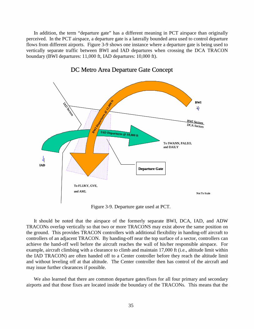
35

In addition, the term “departure gate” has a different meaning in PCT airspace than originally perceived. In the PCT airspace, a departure gate is a laterally bounded area used to control departure flows from different airports. Figure 3-9 shows one instance where a departure gate is being used to vertically separate traffic between BWI and IAD departures when crossing the DCA TRACON boundary (BWI departures: 11,000 ft, IAD departures: 10,000 ft).

Figure 3-9. Departure gate used at PCT.

It should be noted that the airspace of the formerly separate BWI, DCA, IAD, and ADW TRACONs overlap vertically so that two or more TRACONS may exist above the same position on the ground. This provides TRACON controllers with additional flexibility in handing-off aircraft to controllers of an adjacent TRACON. By handing-off near the top surface of a sector, controllers can achieve the hand-off well before the aircraft reaches the wall of his/her responsible airspace. For example, aircraft climbing with a clearance to climb and maintain 17,000 ft (i.e., altitude limit within the IAD TRACON) are often handed off to a Center controller before they reach the altitude limit and without leveling off at that altitude. The Center controller then has control of the aircraft and may issue further clearances if possible.

We also learned that there are common departure gates/fixes for all four primary and secondary airports and that those fixes are located inside the boundary of the TRACONs. This means that the

IAD

BWI

DC Metro Area Departure Gate Concept

Not To Scale

BW

I D

epar

ture

s @

11,

000

ft

IAD Departures @ 10,000 ft

BWI SectorsDCA Sectors

IAD

Sectors

Departure Gate

To SWANN, PALEO, and DAILY

To FLUKY, GVE,

and AML

IAD

BWI

DC Metro Area Departure Gate Concept

Not To Scale

BW

I D

epar

ture

s @

11,

000

ft

IAD Departures @ 10,000 ft

BWI SectorsDCA Sectors

IAD

Sectors

Departure Gate

To SWANN, PALEO, and DAILY

To FLUKY, GVE,

and AML

36

TRACON departure controllers are responsible for merging departure flows over those fixes. There are nine major departure fixes:

• East: SWANN (primarily jets, heavy afternoon pushes including international flights), and PALEO (some turboprops);

• Southeast: DAILY (light traffic);

• Southwest: HAFNR, and FLUKY;

• West: LDN, and AML271030 (created for TAAM simulation purpose);

• Northwest: BUFFR, and JERES.

Although the in-trail separation standard is 5 nautical miles, a survey of the TRACON and ARTCC controllers revealed that the spacing generally ranges from 7 to 10 nautical miles in practice due to the lack of a precise control tool or spacing method. The TRACON controllers on the average give 7 nm. Center controllers, on the other hand, generally believe that 7 nm is too close and tend to prefer as much as 10 nm. Generally though, the center controllers think the number should be between 8 and 9 nm for en route flights (where speeds are more stabilized). The spacing methods that PCT controllers use are altitude change, vectoring, and speed control. Most of the time, one method is preferred over the others. Among the three common actions, speed control is probably the least favored method. During busier times, it is easier to adjust altitude, so altitude change is probably the most popular method among PCT controllers. For spacing departure aircraft that merge into en route streams, vectoring is often used in order to accommodate the required in-trail separation for aircraft flying at about the same speed. For example, westbound departures from IAD and DCA joining jet route J149 are merged to the west of IAD. Aircraft departing DCA are advised to head southwest first and to cross the DCA/IAD TRACON boundary at or above 11,000 ft, and then turn right, heading northwest, and finally to merge with jet route J149.

All four major airports in the DC metro area have dual-use runways. For example, during a NNNW flow pattern7, 01L and 01R at ADW, 01, 03, and 33 at DCA, 01L and 01R at IAD, and 33R at BWI are used for both departure and arrival purposes.

We learned during the site visit to the Washington DC area that neither the TRACON nor the Center is responsible for separating trans-Atlantic flights. Those flights are spaced when they near the oceanic fixes in the NY center airspace. Therefore, PCT would not be able to experience this targeted EDP benefit.

Economic Conversion The ground departure time (including taxi-out time and delays in lineup queue, and takeoff run

time) and the airborne time of major DC airport departure flights, and the ground arrival time

7 North flow at ADW, DCA, and IAD, and west flow at BWI.

37

(including taxi-in time and landing roll time) and airborne time of the arrival flights are compared between the baseline, climb, merge, and combined EDP simulations. The aircraft are grouped into the following categories: four engine wide body jet, four engine narrow body jet, three engine wide body jet, three engine narrow body jet, two engine wide body jet, two engine narrow body jet, turboprop with under 20 seats, turboprop with 20 or more seats, piston with one engine, and pistons with two engines weighing less or more than 12,500 pounds, etc. This procedure is performed using information from Appendix A (Aircraft Information Fixed Wing) of FAA Order 7110.65M (ref. 17) and Appendix A (Aircraft Types) of reference 2. Fixed wing aircraft designators information in the FAA’s Altoona Automated Flight Service Station (ref. 29) is also used to identify some types of aircraft. The differences in airborne time were then converted to dollar values using the airborne time economic conversion factors from the FAA’s guide for evaluation of investment and regulatory programs (ref. 16) and Appendix B (Economic Conversion Factors) of reference 28 (see Table 3-4). Conversion from ground time savings to dollars is more problematic because no official reference is available. By studying the fuel consumption rates during cruise and taxi for a number of aircraft, we derived that the average ratio of the two rates is 1.7 (ref. 18). This factor is used to obtain taxi fuel and oil cost from the fuel and oil cost given in the FAA’s guide. It is assumed that the crew cost and maintenance costs are the same for cruise and taxi (see Table 3-5). The referenced economic conversion factors, originally in 1996 and 1997 dollar amounts, are converted to year 2000 dollars using the Consumer Price Index (CPI) values published by the Bureau of Labor Statistics of the Departure of Labor (ref. 30).

Table 3-4. Economic conversion factors for airborne hours (refs. 16 and 2) (year 2000 $).

Per Airborne Hour Cost ($/hr) Economics Values Class

Crew Fuel & Oil Maintenance

Total

Two Engine Narrow Body Jet $1,018 $730 $565 $2,314Two Engine Wide Body Jet $1,634 $1,264 $856 $3,755Three Engine Narrow Body Jet $1,304 $1,125 $781 $3,210

Three Engine Wide Body Jet $2,174 $2,005 $1,601 $5,781

Four Engine Narrow Body Jet $639 $910 $1,087 $2,635

Four Engine Wide Body Jet $2,731 $2,967 $1,865 $7,562

Turboprops Under 20 Seats $164 $127 $157 $448

Turboprops Over 20 Seats $250 $159 $349 $758

Piston 1 Engine $63 $29 $32 $124

Piston 2 Engine < 12500 lbs. $83 $74 $91 $248

Piston 2 Engine > 12500 lbs. $83 $86 $99 $268

8 Mainly used for grouped piston aircraft (Piston 1 Engine, Piston 2 Engine < 12500 lbs, and Piston 2 Engine > 12500 lbs, etc.); ref. 16 only has specific piston aircraft listed. Block hour conversion factors for piston aircraft in reference 2 were used.

38

Table 3-5. Economic conversion factors for ground hours (year 2000 $).

Per Ground Hour Cost ($/hr) Economics Values Class

Crew Fuel & Oil (/1.7) Maintenance Total

Two Engine Narrow Body Jet $853 $358 $471 $1,681Two Engine Wide Body Jet $1,479 $672 $774 $2,925Three Engine Narrow Body Jet $1,078 $543 $642 $2,263

Three Engine Wide Body Jet $1,951 $1,058 $1,438 $4,447

Four Engine Narrow Body Jet $519 $435 $881 $1,835

Four Engine Wide Body Jet $2,578 $1,647 $1,760 $5,986

Turboprops Under 20 Seats $125 $574 $121 $303

Turboprops Over 20 Seats $199 $74 $274 $547

Piston 1 Engine $63 $17 $32 $112

Piston 2 Engine < 12500 lbs. $83 $43 $91 $217

Piston 2 Engine > 12500 lbs. $83 $50 $99 $232

Direct EDP benefits are expected to be in the form of reduced airborne time of the departure flights. Thus, the converted airborne values for all DC area departure flights are summed to yield the direct potential benefit of EDP. When operated together with a surface DST such as SMS, EDP is also expected to help reduce departure queue delay/taxi delay. This indirect form of savings is reflected in the converted ground values for departure flights.

3.5.3. Benefit Extrapolation Methodology

Once the potential EDP benefits for a typical day in 2005 at the Washington site are assessed, they are first annualized to that full year. This is done by simply multiplying the daily value by 365:

365,2005, ×= DailyPCTPCT BB

Where: 2005,PCTB is the total annual potential benefit of EDP at PCT in the year 2005.

DailyPCTB , is the total daily potential benefit of EDP at PCT in the year 2005.

This annual benefit value is then used as the basis for extrapolation to other sites and for other years. To do that, we assumed that the benefit is directly proportional to the Relative Potential Benefit (RPB) values at a site for the years it is assumed to have EDP in operation. Relative Potential Benefit values are calculated using the procedure outlined in Section 3.2. For the projected volume of total operations at an airport, this report uses the number published in the FAA’s Terminal Area Forecast (TAF, ref. 11). The TAF published in 2003 only predict to the year 2020. However, demand forecasts for all airports are linear after 2015, thus we assume this trend will be maintained beyond 2020. The benefit extrapolation method can be expressed by the equation:

2005,,2005,, / PCTjiPCTji RPBRPBBB ×=

39

Where: jiB , is the total annual potential benefit of EDP at site “ i ” in year “ j ”.

jiRPB , is the Relative Potential Benefit of EDP at site “ i ” in year “ j ”.

For a given site and year, the EDP benefits are assumed to be either zero, or the full, annualized value obtained from the benefit assessment methodology. Benefits of EDP during TRL 1 to TRL 6 development and during technology transfer were not included in the assessment. So, for each site it is assumed that when EDP reaches PCA (Planned Capability Available) during a given year, then that year is the first year that will produce benefits. This LCCBA analysis is performed with a granularity of one-year. Although the granularity of the timing of benefits could be made smaller, a finer granularity is not justified, considering the precision of this study.

3.6. Life-Cycle Cost/Benefit

Two deployment scenarios were considered by this assessment: a full 14-site deployment and a partial, 9-site scenario. We will consider both direct and indirect EDP potential benefits for each scenario. The following types of LCCBA results are provided for all cases studied:

• Annual Costs and Benefits.

• Net Present Value (NPV): This is the difference between the discounted present value of benefits and the discounted present value of costs. Discounting is a method of evaluating an investment by estimating future cash flows and taking into consideration the time value of money. The present value of benefits and costs is the base-year-value of the benefits and costs over the various years discounted at an appropriate discount rate. If profitable, an investment will have a NPV greater than zero.

• Benefit to Cost ratio (B/C ratio): This is the ratio of the present value of benefits to the present value of costs. This ratio must be greater than 1 to justify a project. A DST with higher benefit to cost ratio is a better investment option than a DST with a lower benefit to cost ratio.

• Break Even Point (BEP): The break-even point is the year at which the DST's net present value of benefit just equals its net present value of cost. Generally, it is the time required to recoup the initial investment made for acquiring and implementing the alternative technology.

As part of the LCCBA methodology, it is important to determine the base year of analysis, the economic service life (ESL) of the system, and the discount rate for NPV calculations. If the estimated costs are not assessed at the base year dollar values, then conversion to base year costs requires knowledge of the deflation/inflation rate. These parameters used by this report are discussed next.

• All costs and benefits are to be expressed in year 2000 dollars.

• Costs to date (year 2003) are to be considered sunk costs and, in accordance with OMB Circular A-94 (ref. 19), are not considered in the LCCBA.

40

• The discount rate will be 7%, as per OMB Circular A-94 (ref. 19).

• In the LCCBA, the deflation/inflation rate is assumed to be the same as the CPI (ref. 30), and EDP is assumed to have an ESL of 20 years (ref. 28).

As mentioned before, this assessment is of potential costs and benefits and not of actual costs and benefits. The likelihood that the DST will be able to achieve the potential costs and benefits was not analyzed in this report.

An added analysis for this study, requested by the EDP developers, is to “break-up” the EDP costs by year 2000 normalized EDP Relative Potential Benefit ratios as shown in Table 3-3. This will enable a site-by-site cost/benefit analysis. We did not justify the validity of this cost appropriation method; these results are only provided as a reference.

41

4. TAAM SIMULATION AND BENEFITS ANALYSIS

4.1. Benefits Assessment Simulations

This section begins by describing some details of the TAAM simulation models used in this study. Simulation results will be given in Section 4.2.

4.1.1. Characteristics of TAAM Simulation Models

The baseline TAAM model used in this study was derived from the model that the FAA used to conduct the Environmental Impact Study before the consolidation of TRACONs BWI, IAD, DCA, and ADW into PCT. As received from the FAA, the simulation satisfactorily modeled the traffic of the Washington DC area for a typical day in the 2005 time frame. Our FAA contact at the Potomac TRACON believes that the model reflects the real traffic situation. The creation of the model was documented in detail by the FAA (ref. 20). Their effort going into preparation of the baseline traffic schedule along with descriptions of typical traffic flow patterns around the major DC area airports will be briefly discussed.

The operating details essential to air traffic simulation include types of operations (Air Carrier, Air Taxi, General Aviation and Military, or AC, AT, GA and M), aircraft type(s), traffic routes, radar ground track(s), fix loading by operation type, and traffic volume variability. The Potomac TRACON (PCT) Airspace Team (PAT) gathered this information to construct their Potomac TAAM simulation models.

During development of the Potomac air traffic simulations by the PAT, the diurnal traffic patterns were characterized and extrapolated to support development of an engineered day of traffic. This engineered day approach was sufficiently developed to address routing detail where aircraft enter and leave the terminal ATC environment. Assessment of actual traffic flown over a number of days was effected to determine the fraction of aircraft utilizing the arrival and departure fixes of the individual airports. Traffic volume was then assessed from historical records to arrive at a 90th percentile aircraft volume day for each type of operation (AC, AT, GA and M), for each facility.

The three primary DC metro area airports and ADW operate in various airport configurations, depending on weather patterns and facility demand. The pattern of operations occurring on the airport’s runways is referred to as the airport’s configuration, and is typically designated by directions of the traffic flow. For example, configurations of each of the four basis airports in PCT are typically designated as North, South, East, or West. Thus, a number of TRACON-wide combinations of airport configurations are possible, given that each of the basis airports can have at least four configurations. However, most TRACON configurations are rarely used due to the proximity of, and therefore, interdependence of the basis airports. The PAT team decided that the most representative TRACON configurations would be North/North/North/West and South/South/South/East for ADW/DCA/IAD/BWI, with the first of these configurations slightly dominant. For the assessment of potential EDP benefits, we chose to use only the first configuration and assume that it is representative. The runway usage under this TRACON configuration is listed in Table 4-1.

42

Table 4-1. Runway usage under a North/North/North/West TRACON configuration.

Major Airports Runways Usage

01L Mixed ADW

01R Mixed 28 Departure 33L Arrival BWI 33R Mixed 03 Mixed 33 Mixed DCA 01 Mixed 01L Mixed 01R Mixed IAD 30 Departure

After determining the airspace and runway configurations for the engineered day, the visual approach procedures in the terminal environment for each airport were modeled by the FAA. For the traffic volume, Enhanced Traffic Management System (ETMS), Automated Radar Terminal System data, as well as the Official Airline Guide were assessed to ensure complete coverage of city-pair traffic. Individual aircraft flight operating norms with city pair, routing, aircraft type, and schedule were characterized from actual ETMS traffic observations spanning several days9. The 90th percentile traffic volume (from 1998 statistics) was correlated with operations types (AC, AT, GA and M) for each primary facility and secondary, or satellite airports from this ETMS data to arrive at 1998 “source” flight data. This “source” flight data was then escalated to project traffic in future years, e.g., 2005. This forecasting considered socioeconomic trends, domestic airfare trends, and passenger air traffic trends, and used a bottom-up approach to develop the passenger and cargo aircraft forecast. This forecast provides the daily operations for all aircraft flying IFR arriving at and departing from all airports in the greater Baltimore-Washington area. In addition to the four basis airports, 26 satellite airports were also included. Specifically for ADW, BWI, DCA, and IAD, forecasted daily operation in a typical day in 2005 is shown in Table 4-2. The fleet mix of the 4200 arrivals and departures at the four basis airports is given in Table 4-3, broken down by the economic value class. There are 9 major departure fixes used by the Potomac TRACON (see Section 3.5.2). Their utilization by Washington area departure fixes is shown in Figure 4-1.

To minimize interruption of traffic flow, the engineered day’s traffic actually continues into the second day. However, the number of operations beyond 24-hours is insignificant. Furthermore, these operations do not show noticeable benefits due to the use of EDP. Hence, this report assumes that the engineered day equals a calendar day when performing benefit annualization. Extrapolating this engineered day’s traffic volume yields higher annual traffic counts than that from the FAA TAF (ref. 11). This is because it represents the 90th percentile day’s traffic (37th busiest day). Due to the uncertainties in forecasting future traffic amounts, we did not perform further analysis on this matter.

9 According to reference 20, these days are 11/19/98, 11/20/98, 11/24/98, and 11/25/98.

43

There were a total of 153 Standard Instrument Departures (SIDs) included in the TAAM simulation model, which corresponded to operating procedures and radar tracks. Most SIDs corresponded to the nine departure fixes. Likewise, 124 Standard Terminal Arrival Routes (STARs) were used to describe the paths flown by the arrival flights from the arrival fixes to the heads of the runways. The separation of departure/arrival streams, and sometimes departure/departure streams was controlled by setting altitude restrictions on appropriate SIDs and STARs. There were 279 “Do Not Climb Above” restrictions within the 153 SIDs. Sometimes there were as many as 5 such clauses for a single SID, and it was common to have four. The presence of these restrictions reflects the complexity of operations in the Potomac TRACON.

Table 4-2. Runway activity for an engineered day in 2005.

Airport Runway Departure Operations Arrival Operations Totals 01L 54 54 10801R 73 73 146ADW

Subtotals 127 127 25433L 0 379 37933R 116 131 24728 388 0 388

BWI

Subtotals 504 510 1,014

01 287 341 62803 122 49 17133 99 120 219

DCA

Subtotals 508 510 1,018

01L 180 540 72001R 346 420 76630 428 0 428

IAD

Subtotals 954 960 1,914

Table 4-3. Fleet mix of engineered day in 2005.

Economics Values Class Number of Departures Number of Arrivals

Two Engine Narrow Body Jet 1,585 1,594Two Engine Wide Body Jet 44 44Three Engine Narrow Body Jet 33 37Three Engine Wide Body Jet 9 9Four Engine Narrow Body Jet 11 11Four Engine Wide Body Jet 22 21Turboprops Under 20 Seats 86 78Turboprops Over 20 Seats 214 213Piston 1 Engine 36 46Piston 2 Engine < 12500 lbs. 53 54Piston 2 Engine > 12500 lbs. 0 0

44

Figure 4-1. Departure fixes utilization.

4.1.2. Simulation Model Descriptions

Only a few, minor modifications were made to the FAA model to allow it to serve as the baseline model for this assessment. Most of these modifications were necessary to resolve software compatibility issues that developed in the interim since the model was last used. However, four changes were required for more substantial reasons:

• The original FAA simulation model did not use in-trail separation. Using the information we gathered during the visit to the Potomac TRACON and the Washington ARTCC, we enabled the in-trail separation function in TAAM and used 8 miles in-trail for the nine major departure fixes to represent current operations (see Figure 4-1 for the names of these fixes).

• The original FAA simulation model mistakenly used slightly different values for desired final approach speeds at the four major DC area airports. When these airports are “combined” in the simulation of EDP’s merge advisories, only one value can be used. As a result, arrival operations at an airport would be penalized or favored unrealistically. Thus, the desired final approach speed settings at DCA, BWI, and ADW were adjusted to the same values as those at IAD.

SWANN

PALEO

402

215

DAILY178

HAFNR

FLUKY

173

165

LDN

AML271030167

272

JERES

BUFFR

189

75

BWI

ADWDCA

IAD

SWANN

PALEO

402

215

DAILY178

HAFNR

FLUKY

173

165

LDN

AML271030167

272

JERES

BUFFR

189

75

BWI

ADWDCA

IAD

BWI

ADWDCA

IAD

45

• We learned from the EDP developers that EDP should not have significant influence on arrivals. To simulate this characteristic to a degree of satisfaction, the “landing queue threshold,” “sequencing action threshold,” and the “sequencing fixed threshold” settings of the four basis DC metro area airports (IAD, DCA, BWI, and ADW) were adjusted.

• Based on software manufacturer’s recommendation, the sharp turns used in the original SIDs were rounded to improve simulation fidelity.

In spite of all these changes, the averaged flight times of the EDP study baseline model did not stray significantly from the original FAA model.

The FAA simulation does not have detailed ground traffic modeled at any airports. Excepting IAD, airports do not have gates, aprons, taxiways, etc. No usage rules exist at any airports. Ideally, ground traffic simulation is needed to evaluate taxi delay savings. However, we did not have the time during this project to accomplish this.

Expedited Climb Profiles Simulation Model The expedited climb profiles of EDP was simulated using the following two measures:

1. Remove altitude restrictions from the SIDs.

As mentioned earlier, the baseline model contains Standard Instrument Departures (SIDs) that were constructed according to operating procedures and traffic observation data. The “tunneling,” “capping,” or “shelving” of traffic streams are enforced by altitude restrictions on the SIDs. Thus, one measure we took to simulate the expedite climb of EDP was to remove these restrictions. One such SID (from runway 01R at IAD to departure fix SWANN) is given as an example below (Figure 4-2), with the highlighted clauses denoting the removed restrictions in the EDP simulation:

Figure 4-2. Example SID with altitude restrictions.

Maintain runway heading When crossing 40 deg radial AML VOR turn auto track directly to IA01R VOR At 0.0 DME IA01R turn auto track directly to I010 VOR At 0.0 DME I010 turn auto track directly to I011 VOR At 0.0 DME I011 turn auto track directly to I090 VOR At 0.0 DME I090 turn auto track directly to B019 VOR At 0.0 DME B019 turn auto track directly to POT508 VOR At 0.0 DME POT508 turn auto track directly to A001 VOR At 0.0 DME A001 turn auto track directly to W094 VOR At 0.0 DME W094 turn auto track directly to SWANN VOR Reach 5500 ft or above by I010 VOR Reach 10000 ft or above by I090 VOR Do not climb above 10000 ft until 0.0 DME POT508 Reach 11000 ft or above by A001 VOR Reach 14000 ft or above by W094 VOR Do not climb above 19000 ft until 0.0 DME SWANN

46

2. Remove altitude restrictions from the flight plan.

Similarly, there might be altitude restrictions in the flight plan for a specific flight. In such a case, the altitude restriction at the departure fix (the first waypoint of the flight plan in TAAM is always the departure fix) is removed. One such example is shown in Figure 4-3.

Figure 4-3. Example flight plan entry with altitude restrictions.

Precision Spacing Simulation Model To improve conflict checking and coordinate departure runways at different airports, we

replaced the TAAM models of the four major airports with a composite airport: “Washington Combined,” or WAS, in TAAM. WAS contains all the runways at IAD, DCA, BWI, and ADW. Under the nominal NNNW flow pattern, these runways are: 01L, 01R, and 30 (IAD), 01, 03, and 33 (DCA), 04, 28, 33L, and 33R (BWI), 01L and 01R (ADW10). In a nutshell, this process involves the following steps11:

1. Create an airport with the above-mentioned runways. The airport properties that must be resolved are the geographic coordinates, the surface elevation, and the local magnetic declination. The latitude and longitude of the new airport were taken to be that of IAD. Because TAAM only uses these coordinates for preflight calculation, they will not impact simulation results. To obtain surface elevation and magnetic declination, traffic-weighted averages of values from the four basis Washington airports were used.

2. Establish correct relationships between runways (e.g., 01L, originally of IAD, and 01, originally of DCA should operate independently).

3. Modify the route file to be consistent with the combined airport.

4. Modify the flight plans to be consistent with the combined airport.

10 Because TAAM does not support two runways at the same airport having the same designation, the ADW runways were renamed to 02L and 02R in this simulation model.

11 The actual procedures are rather technical and will not be described in detail here.

UAL1038_E B777 KIAD-EBBR.J 310 01,22:15, 02,05:25 @SID ? ? @STAR ? ? @R KIAD-EBBR.J

KIAD ? 0 0 0 SWANN 19000 0 0 0 GOLDA 21000 0 0 0 BROSS 23000 0 0 0 OOD ? 0 0 0

…

47

5. Modify runway usage rules so that they are consistent with those in the baseline model.

6. Create new runway usage rules so that departures and arrivals behave appropriately.

7. For flights between the four basis airports, the use of runways (departure and/or arrival) is adjusted in flight plans to match baseline simulation results.

As described in Section 3.5.2, another measure required to simulate the precision spacing mechanisms of EDP is simply reducing the miles-in-trail restriction at the departure fixes. However, NASA’s EDP developers did not provide us with a miles-in-trail value that EDP is expected to achieve. Although we attempted to obtain as-flown in-trail separation distributions from ETMS data covering the Washington D.C. area, the ETMS data proved to be too sparse in the vicinity of departure fixes to yield meaningful aircraft separation targets. It was then decided, with the consensus of the EDP developers, to model the performance of EDP in achieving in-trail separation by assuming that the in-trail separation distribution for departures is similar to the inter-arrival separation at the runway head. In a recent aFAST potential benefit assessment performed (ref. 21), examination of traffic observation data at DFW showed that the best spacing achieved during VMC is a near normal distribution with a mean of 3.5 nautical miles for large-large pairs of aircraft. This is achieved when the standard wake turbulence separation between a pair of large aircraft under dry runway conditions is 2.5 nautical miles. The aFAST potential benefit alternatives considered in reference 21 include matching this best-observed VMC inter-arrival distance separation (mean and standard deviation), and reducing the mean and/or the standard deviation. However, it was found by reference 21 that reducing the standard deviation (spread) of the distribution did not bring any noteworthy monetary benefits for aFAST. One of the aFAST potential benefit alternatives is to match the observed proportions below the wake turbulence standard, equivalent to a distribution with mean inter-arrival separation at 3.2 nautical miles (nmi).

In this report, we decided somewhat arbitrarily that EDP would mimic this aFAST alternative. Because the in-trail separation standard is 5 nautical miles, the one EDP potential benefit alternative we considered in this assessment is then reducing the in-trail separation setting from 8 nmi to 6.4 nmi (3.2 × 5/2.5).

Combined EDP Simulation Model The above models were combined to evaluate the effect of the three EDP benefit mechanisms,

namely, expedite climb profiles, precision spacing, and improved departure sequencing.

From here forward, these three TAAM models (simulations) will be called EDP-Climb, EDP-Merge, and EDP-Both, while the EDP study Baseline model will be simply called the Baseline.

4.2. Simulation Results

4.2.1. Baseline Simulation Results

TAAM classifies an aircraft’s simulated flight time into the following 5 categories: Gate Delay, Ground Departure Time, Airborne Time, Ground Arrival Time, and Total Time.

48

• Gate Delay: Total delay at the gate, including departure sequencing delays; delayed pushback due to traffic in apron area; arrival sequencing and flow control at destination airports, runway congestion; delays due to late arrival of next linked flight, etc.

• Ground Departure Time: The sum of taxi-out time and takeoff roll time. Taxi-out time includes movement time and delays in the lineup queue and at taxiway intersections.

• Airborne Time: Total time from wheels-off until touchdown. This includes delays due to speed control, airborne holding, radar vectoring, altitude changes, and path stretching.

• Ground Arrival Time: The sum of landing roll time and taxi-in time. Taxi-in time includes movement time, delays at taxiway intersections, and standoff delays if the arrival gate wasn't immediately available.

• Total Time: The sum of the above four times, i.e., gate-to-gate time plus gate delay.

We summed up the above 5 categories of time for all 6,402 flights and compared them between the EDP study Baseline (Baseline) and the FAA simulation (FAA) in Table 4-4. In addition, the cumulative total times for all departure and arrival operations of the 4 basis airports are also listed in the table. As can be seen, the major mismatch between the models is in the Ground Departure Time of the Washington departure flights. It is believed that this difference is artificial, and due to differences in simulation environments (mainly TAAM version and common/static file issues), and changes made to the model to ensure proper simulation of EDP functions. Also notice the difference in the Airborne Time of the Washington arrival flights. This is primarily due to the difference of the desired final airspeed used (see Section 4.1.2). However, even with these differences, the average discrepancy is insignificant (about 16 seconds per Washington flight).

Table 4-4. Baseline and FAA simulation flight times (h:mm:ss).

Simulation Gate DelayGround

Departure Airborne

Ground Arrival

Total

FAA 0:03:46 180:46:57 9737:22:09 24:30:08 9942:43:01All

Baseline 0:05:03 166:40:52 9730:28:30 24:24:06 9921:38:31FAA 0:00:00 176:27:43 2803:49:27 3:50:50 2984:08:01Washington

Departures Baseline 0:00:00 161:46:57 2801:29:16 3:46:06 2967:02:19FAA 0:03:46 3:09:47 2945:58:20 16:10:30 2965:22:23Washington

Arrivals Baseline 0:05:03 3:00:24 2944:06:56 16:09:36 2963:21:59

The numbers of departures and arrivals in 10-minute bins for the 4 basis airports of our baseline and the FAA model are compared in Figures 4-4 through 4-11, and show good agreement.

49

Figure 4-4. ADW departure comparison (Baseline vs. FAA).

Figure 4-5. ADW arrival comparison (Baseline vs. FAA).

0

1

2

3

4

5

6

0:00 2:00 4:00 6:00 8:00 10:00 12:00 14:00 16:00 18:00 20:00 22:00 0:00 2:00

Time

Fre

qu

en

cy

(c

ou

nt

of

flig

hts

)Baseline

FAA

0

1

2

3

4

5

6

0:00 2:00 4:00 6:00 8:00 10:00 12:00 14:00 16:00 18:00 20:00 22:00 0:00 2:00

Time

Fre

qu

en

cy

(c

ou

nt

of

flig

hts

)

Baseline

FAA

50

Figure 4-6. BWI departure comparison (Baseline vs. FAA).

Figure 4-7. BWI arrival comparison (Baseline vs. FAA).

0

1

2

3

4

5

6

7

8

9

10

0:00 2:00 4:00 6:00 8:00 10:00 12:00 14:00 16:00 18:00 20:00 22:00 0:00 2:00 4:00

Time

Fre

qu

en

cy

(c

ou

nt

of

flig

hts

)

Baseline

FAA

0

2

4

6

8

10

12

0:00 2:00 4:00 6:00 8:00 10:00 12:00 14:00 16:00 18:00 20:00 22:00 0:00 2:00 4:00 6:00

Time

Fre

qu

en

cy

(c

ou

nt

of

flig

hts

)

Baseline

FAA

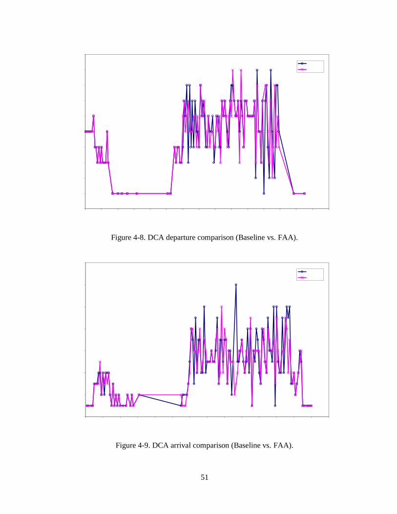
51

Figure 4-8. DCA departure comparison (Baseline vs. FAA).

Figure 4-9. DCA arrival comparison (Baseline vs. FAA).

0

1

2

3

4

5

6

7

8

9

10

0:00 2:00 4:00 6:00 8:00 10:00 12:00 14:00 16:00 18:00 20:00 22:00 0:00 2:00 4:00 6:00

Time

Fre

qu

en

cy

(c

ou

nt

of

flig

hts

)

Baseline

FAA

0

2

4

6

8

10

12

14

0:00 2:00 4:00 6:00 8:00 10:00 12:00 14:00 16:00 18:00 20:00 22:00 0:00 2:00 4:00

Time

Fre

qu

en

cy

(c

ou

nt

of

flig

hts

)

Baseline

FAA

52

Figure 4-10. IAD departure comparison (Baseline vs. FAA).

Figure 4-11. IAD arrival comparison (Baseline vs. FAA).

0

5

10

15

20

25

30

0:00 2:00 4:00 6:00 8:00 10:00 12:00 14:00 16:00 18:00 20:00 22:00 0:00 2:00 4:00

Time

Fre

qu

en

cy

(c

ou

nt

of

flig

hts

)

Baseline

FAA

0

2

4

6

8

10

12

14

16

18

0:00 2:00 4:00 6:00 8:00 10:00 12:00 14:00 16:00 18:00 20:00 22:00 0:00 2:00 4:00 6:00 8:00 10:00 12:00

Time

Fre

qu

en

cy

(c

ou

nt

of

flig

hts

)

Baseline

FAA

53

4.2.2. EDP Expedited Climb Profiles Simulation Results

Total simulated flight times are compared between the EDP Expedited Climb Profiles simulation and the Baseline (see Table 4-5). It can be seen that the EDP simulation used less airborne time and ground departure time for the Washington departures—the savings are 9.7 and 1.1 hours, respectively. When averaged, these are about 17 and 2 seconds per departure. The savings in the air result from removal of altitude restrictions from the SIDs and flight plans based on EDP’s direct climb advisory. This is evident when comparing the times and distances between take off and achievement of cruise altitude between the two simulations (see Table 4-6). Figures 4-12 and 4-13 graphically depict the distribution of these differences. On the average, there is a reduction in time to reach cruise altitude of 1.2 minutes (about 6.7 nautical miles) per departure.

Table 4-5. EDP-Climb and Baseline simulation flight times (h:mm:ss).


Departure Airborne

Ground Arrival

Total

Baseline 0:05:03 166:40:52 9730:28:30 24:24:06 9921:38:31All

Climb 0:05:03 165:33:22 9720:49:30 24:24:06 9910:52:01Baseline 0:00:00 161:46:57 2801:29:16 3:46:06 2967:02:19Washington

Departures Climb 0:00:00 160:39:15 2791:48:46 3:46:06 2956:14:07Baseline 0:05:03 3:00:24 2944:06:56 16:09:36 2963:21:59Washington

Arrivals Climb 0:05:03 3:00:24 2944:06:20 16:09:36 2963:21:23

Table 4-6. Time and distance to cruise altitude comparison (Baseline – EDP-Climb).

Baseline Climb Savings

Time (min.) 18.8 17.6 1.2Average

Distance (nmi) 97.5 90.8 6.7Time (min.) 50.3 25.9 24.4

Max. Savings Distance (nmi) 158 58 100

Time (min.) 39,347 36,797 2,550Total

Distance (nmi) 203,832 189,829 14,003

Figure 4-14 and Figure 4-15 show average Altitude-Time and Altitude-Distance profiles, respectively. Figure 4-16 and Figure 4-17 contrast extreme cases of the respective profiles. The absence of “level-off” during the ascent phase of the simulated EDP Expedite Climb flights can be clearly seen in each case. As a side effect, departure queue delays/taxi delays were also reduced due to EDP’s direct climb advisory. This is probably because direct climb better separates departing aircraft vertically, thus enabling those flights to take off that, without EDP, would have been held on the ground due to airspace congestion. On the other hand, arrival flights were essentially not affected in the EDP-Climb simulation; neither the total airborne nor ground arrival time changed from that of the Baseline’s values.

54

Figure 4-12. Flight distribution of time to cruise altitude differences.

Figure 4-13. Flight distribution of distance to cruise altitude differences.

0

100

200

300

400

500

600

700

800

-75 -60 -45 -30 -15 0 15 30 45 60 75

nautical miles saved

Fre

ue

nc

y (

co

un

t o

f fl

igh

ts)

0

100

200

300

400

500

600

700

800

900

-18 -14 -10 -6 -2 2 6 10 14 18

minutes saved

Fre

qu

en

cy

(c

ou

nt

of

flig

hts

)

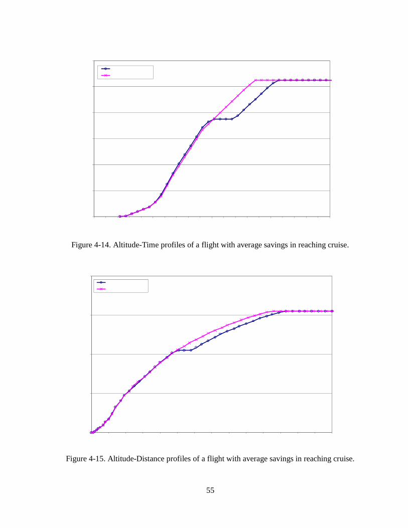
55

Figure 4-14. Altitude-Time profiles of a flight with average savings in reaching cruise.

Figure 4-15. Altitude-Distance profiles of a flight with average savings in reaching cruise.

0

10000

20000

30000

40000

0 20 40 60 80 100 120 140

Distance (nmi)

Alt

itu

de

(ft

)

USA3014_E-Baseline

USA3014_E-Climb

0

4000

8000

12000

16000

20000

24000

1:00 1:05 1:10 1:15 1:20

Time

Alt

itu

de

(ft

)DAL3002_E-Baseline

DAL3002_E-Climb

56

Figure 4-16. Altitude-Time profiles of the flight with the most savings in reaching cruise.

Figure 4-17. Altitude-Distance profiles of the flight with the most savings in reaching cruise.

0

4000

8000

12000

16000

20000

24000

28000

32000

11:55 12:00 12:05 12:10 12:15 12:20 12:25 12:30

Time

Alt

itu

de

(ft

)

S60206-Baseline

S60206-Climb

0

4000

8000

12000

16000

20000

0 20 40 60 80 100 120

Distance (nmi)

Alt

itu

de

(ft

)

N600DT#2-Baseline

N600DT#2-Climb

57

4.2.3. EDP Precision Spacing Simulation Results

Total simulated flight times were compared between the EDP Precision Spacing simulation and the Baseline in Table 4-7. Surprisingly, the anticipated savings in the form of reduced airborne times of the Washington departure flights are not seen. It seems that the combined effect of longer look-ahead time and reduced in-trail separation is reduced departure queue delay/taxi delay, a savings of over 11 hours for the 2,093 Washington departure flights, or more than 19 seconds per flight. When the in-trail separation distances for all Washington departures, as measured at the nine departure fixes, are compared between the Baseline and the EDP-Merge simulation, little improvement is observed. This can be seen in Figure 4-18. It is reasoned that this EDP function improved departure scheduling and resulted in reduced ground departure time. We believe that these deviations from the ideal are realistic and will not overestimate potential benefits.

Table 4-7. EDP-Merge and Baseline simulation flight times (h:mm:ss).


Departure Airborne

Ground Arrival

Total

Baseline 0:05:03 166:40:52 9730:28:30 24:24:06 9921:38:31All

Merge 0:03:04 154:33:51 9731:42:24 24:26:42 9910:45:20Baseline 0:00:00 161:46:57 2801:29:16 3:46:06 2967:02:19Washington

Departures Merge 0:00:00 150:30:55 2801:46:12 3:45:42 2956:02:08Baseline 0:05:03 3:00:24 2944:06:56 16:09:36 2963:21:59Washington

Arrivals Merge 0:03:04 1:50:11 2945:20:38 16:12:18 2963:26:11

Figure 4-18. In-trail separation distance comparison (Baseline and EDP-Merge).

0

10

20

30

40

50

60

70

4 7 10 13 16 19 22 25 28 31 34 37 40 43 46 49 52 55 58 61 64 67 70 73 76

In-trail Separation Distance Bin (nmi)

Fre

qu

ency

(co

un

t o

f fl

igh

ts)

Baseline

Merge

58

However, it was hypothesized that there might not be sufficient flights passing each departure fix to appreciably constrain spacing in this simulated scenario. When another site is considered for EDP’s precision spacing function, e.g., New York or Southern California, the sheer number of flights merging over a single fix could probably make a difference, and perhaps reduced airborne time from the reduction of in-trail separation would be observed. To test this hypothesis and create such a constraining case, the departure fixes around the DC area were “combined,” requiring flights previously merging over separate fixes to merge over a single fix (see Table 4-8). This sensitivity case with “loaded” departure fixes was simulated. The simulation time results are shown in Table 4-9, with in-trail separation distance comparison shown in Figure 4-19. It can be seen from the table and figure that, despite additional savings from reduction of departure queue delay/taxi delay, no significant improvements in the air can be observed for the “loaded” scenario. We reason the following as possible explanations:

• A reduction of 1.6 nautical miles in in-trail separation (from 8 to 6.4) lacks overall impact to the flight time. For example, assuming an average flight speed of 240 knots, travel time for 1.6 nmi is only about 24 seconds. Further assuming that 100 flights in the entire simulation (see first peak in Figure 4-19) could experience this savings, this would only have produced a total savings of 40 minutes, which is slightly more than a second when averaged over the 2,093 departures. On the other hand, reduction in in-trail separation from approximately 20 nmi, or 15 nmi (typical MIT constraints during adverse weather conditions) to 7 nmi or 6 nmi would definitely make a difference.

• Higher “loading” at departure fixes may be needed to appreciably constrain spacing. Conventional wisdom in scheduling of flights dictates that controllers always try to avoid high concentrations of traffic over a fix. Furthermore, this is usually a “diverging” situation as most terminal areas have more departure fixes than departure runways. We believe that if the following two conditions can be satisfied, we could see the effect of EDP’s merging advisories on airborne delay savings: 1) fixes loaded to a certain higher degree, and 2) a situation where queuing causes airborne delay. Unfortunately, there was not enough time in this study to further analyze this problem.

Table 4-8. Combination of departure fixes in “loaded” case.

Direction Departure Fix Loaded Departure FixPALEO

East SWANN

SWANN

South DAILY DAILY FLUKY

South WestHAFNR

HAFNR

LDN West

AML271030 LDN

BUFFR North West

JERES JERES

59

Table 4-9. “Loaded” EDP-Merge and “Loaded” Baseline simulation flight times (h:mm:ss).


Departure Airborne

Ground Arrival

Total

Baseline 0:05:03 167:41:46 9733:17:42 24:24:06 9925:28:37All

Merge 0:03:04 154:36:09 9734:15:54 24:26:42 9913:21:08Baseline 0:00:00 162:47:51 2804:18:28 3:46:06 2970:52:25Washington

Departures Merge 0:00:00 150:33:13 2804:19:42 3:45:42 2958:37:56Baseline 0:05:03 3:00:24 2944:06:56 16:09:36 2963:21:59Washington

Arrivals Merge 0:03:04 1:51:47 2945:20:20 16:12:18 2963:27:29

The increased total arrival airborne time is insignificant (see Table 4-7). As a first approximation, arrivals should not be substantially affected by departures. However, things get complicated when dual use runways get involved, as is the case for most of the runways at PCT. Runway availability and delay are the factors dictating runway selection for the arrivals. As the simulation results show, some aircraft changed their landing runway, resulting in different runway utilization (see Table 4-10). When only jet aircraft are considered, there is actually a savings of 28 airborne minutes, suggesting that the faster arriving airplanes could take advantage of the reduced departure queue delay/taxi delay and fill in “gaps” on the runway at the expense of additional airborne delay for slower turboprop and piston aircraft. The same phenomenon was also discovered during an earlier integrated terminal and surface DST preliminary benefit assessment study (ref. 22).

Figure 4-19. In-trail separation distance comparison (“loaded” case).

0

20

40

60

80

100

120

4 7 10 13 16 19 22 25 28 31 34 37 40 43 46 49 52 55 58 61 64 67 70 73 76


Fre

qu

en

cy

(c

ou

nt

of

flig

hts

)

Loaded Baseline

Loaded Merge

60

Table 4-10. Arrival runway usage comparison (number of aircraft).

Airport Runway Baseline Climb Merge Both 01L (mixed use) 54 54 54 54

ADW 01R (mixed use) 73 73 73 7333L (arrival) 379 379 382 382

BWI 33R (mixed use) 131 131 128 12801 (mixed use) 340 340 311 31103 (mixed use) 49 49 43 43DCA 33 (mixed use) 121 121 156 15601L (mixed use) 540 540 551 551

IAD 01R (mixed use) 420 420 409 409

4.2.4. Combined EDP Simulation Results

When the EDP functions (expedite climb profiles and precision spacing) were simulated together, the results were roughly additive. See Table 4-11 and compare the results with Table 4-5 and Table 4-7. The airborne time savings is a little over 10 hours, which is a little more than that observed from EDP-Climb simulation alone. The departure queue delay/taxi delay savings is 11.4 hours—about the same as the EDP-Merge simulation result. Departure flight time savings are 17 seconds per departure in the air and 20 seconds on the ground.

Table 4-11. EDP-Both and Baseline simulation flight times (h:mm:ss).


Departure Airborne

Ground Arrival

Total

Baseline 0:05:03 166:40:52 9730:28:30 24:24:06 9921:38:31All

Both 0:03:04 154:24:57 9721:20:54 24:27:06 9900:16:01Baseline 0:00:00 161:46:57 2801:29:16 3:46:06 2967:02:19Washington

Departures Both 0:00:00 150:22:01 2791:24:36 3:46:00 2945:32:37Baseline 0:05:03 3:00:24 2944:06:56 16:09:36 2963:21:59Washington

Arrivals Both 0:03:04 1:51:53 2945:19:08 16:12:36 2963:26:41

When the in-trail separation distance from this simulation is compared with that from the Baseline and precision spacing simulations (see Figure 4-20), two observations can be made. First, the change in the distribution of in-trail separation distance is rather “uniform.” And secondly, the overall number of aircraft pairs requiring lateral separation decreased, suggesting better utilization of vertical separation. Specifically, there were 112 fewer in-trail separations recorded in this simulation when compared with the Baseline because more aircraft are separated vertically.

61

Figure 4-20. In-trail separation distance comparison (Baseline, EDP-Merge, and EDP-Both).

4.2.5. Conflict Counts

As explained earlier, this study did not use the conflict resolution function of TAAM. Although it was assumed that conflicts would eventually be resolved by controllers, it remains necessary to assure that there will not be a dramatic increase in the number of conflicts during EDP simulations.

It was found that the number of conflicts dropped during the EDP-Climb simulation and increased in the EDP-merge and EDP-Both simulations, as expected. The conflict counts during the EDP-Both simulation again showed the additive property of benefits from the first two simulations. The EDP-Both simulation behaved very similar to the EDP-Merge simulation with regard to conflicts, and only the EDP-Merge simulation will be analyzed here-forth.

The total count of unique conflicts recorded by TAAM during each simulation is shown in Table 4-12. Although even the Baseline simulation recorded 7,007 conflicts, most of the conflicts shown in the table are actually at legal separation. This is because TAAM categorizes conflicts according to its somewhat arbitrary severity rating scale, which ranges between 1 and 6—1 representing the most severe (see Table 4-13). When grouped by TAAM’s severity level, 87% of the 7,007 conflicts recorded are severity level 3 through 6. On the other hand, 72% of the new conflicts during the EDP-Merge simulation are of severity 3 and above. A closer look of the actual conflicts revealed that more than half of the severity level 3 conflicts were actually at 100% separation. Unfortunately, TAAM did not provide a finer grade of conflict classification levels.

0

10

20

30

40

50

60

70

4 7 10 13 16 19 22 25 28 31 34 37 40 43 46 49 52 55 58 61 64 67 70 73 76


Fre

qu

ency

(co

un

t o

f fl

igh

ts)

Baseline

Merge

Both

62

Table 4-12. Conflict count comparison.

Conflicts Change % Change

Baseline 7,007 - - EDP-Climb 6,748 -259 -4% EDP-Merge 7,685 678 10% EDP-Both 7,520 513 7%

Table 4-13. TAAM conflict severity definition.

Severity Definition

1 <20% of available separation 2 20% to 50% of available separation 3 50% to 100% of available separation 4 100% to 120% of available separation 5 120% to 150% of available separation 6 150% to 200% of available separation

It was found that the additional conflicts in the EDP-Merge simulation were concentrated in a few sectors. FEN, GRACOW, IADWARN, and IADSARN account for 541 or 80% of the conflict increase. Out of the 541 new conflicts, 86% of them were between the arrival-arrival pairs of aircraft on final approach.

Generally speaking, although the total number of conflicts increases in the EDP-Merge and EDP-Both simulations, they do not seem to point to a deficiency in the simulations. From the standpoint of realistic air traffic, the EDP simulations are reasonable.

4.3. EDP Benefits Analysis

Using the simulation time difference of relevant flights and the economic conversion factors in Table 3-4 and Table 3-5, the daily and annualized EDP potential benefits for the three simulation cases were calculated. An airport surface DST, such as SMS, is required to be functioning together with EDP in order to achieve the savings on the ground. Thus, the assessed potential EDP benefits were categorized into the following groups:

• Group 1: Without SMS: Include airborne savings for departures only; count any incidental departure queue delay/taxi delay savings as added airborne delays for departures.

As shown in Section 4.2.3, the assessed potential benefit of EDP-Merge is in the form of ground departure delay savings. According to our assumption in Section 3.5.2, these savings would become a liability (increased airborne delays) without a surface DST like SMS. Thus, potential benefits of EDP-Merge w/o SMS will not be calculated. Because of the additive property of EDP-Climb and EDP-Merge benefits, the w/o SMS potential benefits were not assessed for the EDP-Both case.

63

• Group 2: With SMS: including both airborne and ground savings for departures and arrivals.

These results for Potomac TRACON are shown in Table 4-14.

Table 4-14. Potential EDP benefits at PCT calculated from simulation results (Year 2000 $).

2005 Daily 2005 AnnualW/O SMS $18,000 $6.6 M

EDP-ClimbW/ SMS $25,600 $9.3 M

EDP-Merge W/ SMS $27,700 $10.1 MEDP-Both W/ SMS $52,900 $19.3 M

Using the benefit extrapolation methodology stated in Section 3.5.3, these benefits at other airports during other years can be computed. The estimated potential EDP benefits in the year 2005 at the proposed 14 sites for the example scenario are shown in Table 4-15.

Table 4-15. Estimated EDP potential benefits for the year 2005 (Year 2000 $M).

Site ID Climb w/o

SMS Climb w/

SMS Merge w/

SMS Both w/

SMS N90 $9.3 $13.2 $14.3 $27.2SCT $8.6 $12.2 $13.2 $25.3PCT $6.6 $9.3 $10.1 $19.3NCT $4.1 $5.8 $6.3 $12.0C90 $2.3 $3.3 $3.6 $6.8A80 $2.4 $3.4 $3.7 $7.0D10 $1.2 $1.6 $1.8 $3.4D01 $1.0 $1.5 $1.6 $3.0I90 $0.9 $1.3 $1.4 $2.7A90 $0.7 $1.1 $1.1 $2.2D21 $0.7 $0.9 $1.0 $1.9MIA $0.7 $1.0 $1.0 $2.0M98 $0.5 $0.7 $0.8 $1.5PIT $0.5 $0.7 $0.7 $1.4

Total $39.4 $55.9 $60.5 $115.4

64

5. EDP COST ANALYSIS

Life cycle cost estimation of EDP follows the same methodology we used for McTMA in 2002 (ref. 13), with only small modifications made to the Cost Estimating Relationships (CERs) where necessary, in addition to slight changes in grouping cost factors. In 2002, we applied this methodology to the LCC assessment of McTMA, another DST in NASA’s CTAS tool suite. The assessment results were judged by the FAA Free Flight Program metrics team lead to be "at least in the ballpark” and “very realistic” (ref. 13). The LCC assessment methodology addressed the three key cost characteristics: 1) establishing timing of these costs (LCC phase); 2) consideration of all cost types (coverage); and 3) quantification of these costs (estimation).

As shown in Section 4, our simulation results showed that EDP could produce benefits from reduction of departure queue delay/taxi delay, which are only realizable through integrated use of a surface DST such as SMS. It is believed that there will be costs associated with integration of DSTs. That would apply to the all the “w/SMS” cases. Due to lack of information and time, we have not attempted to estimate these costs. These integration costs need to be added in the future to update the LCCBA of the “w/SMS” scenarios.

5.1. LCC Phase

Figure 5-1 schematically depicts a road map of a DST's life cycle from NASA R&D to the end of the program (not to scale). Based on the timeline of events, DST costs were categorized into one-time-only program costs for each site: recurring annual costs, recurring intermittent costs, initial costs specific to certain sites, and termination costs (not considered for EDP). For clarification, the following symbols are assigned to each category.

• One-time-only costs: OC

• Annual program costs: AP

• Initial costs at the first DST site: I1

• Initial costs at the i th DST site (i > 1): I2

• Annual costs at all DST sites: AC

• Intermittent costs at all DST sites: IC

• Termination costs at all DST sites: TC

65

Figure 5-1. Example of a DST life cycle.

The cost factors were associated with a LCC phase (see Table 5-1) and the deployment scheduling methodology was used to determine the timing (year of occurrence) of the costs related to each cost factor. Once these tasks were completed, the timing of the LCC could be determined.

5.2. Coverage of Costs

Costs were modeled using a two-level hierarchical arrangement of cost factors and cost elements. Those costs applicable to EDP are listed in Table 5-1. This table also shows the LCC phase and the cost estimating models used. The abbreviations for the cost estimating models follow:

• Software-related cost estimating: S

• Hardware-related cost estimating: H

• Other (ad hoc) cost estimating: O

Table 5-1. Cost elements and factors quantified in EDP life cycle cost evaluation.

Coverage of costs Cost element Cost factors

Estimation LCC phase

NASA's R&D R&D S or O OC FAA's program management

Program management personnel PMO support – supplies & travels Contract award process IV&V Miscellaneous studies Program management/technical support

O O O O O O

AP AP OC OC OC

I1, I2, AC Technology transfer NASA hand-off to FAA O I1 DST software development

Development Management and administrative support Integrated logistic support Training development

S S & O

O O

I1, I2 I1, I2 I1, I2 I1, I2

Adaptation Management and administrative support Knowledge base: adaptation data Training development

O O O

I1, I2 I1, I2 I1, I2

TR

L 6

Dem

o Si

te I

DU

Dem

o Si

te P

CA

2nd

Site

PC

A

Las

t Si

te P

CA

FA

A P

rogr

am E

nds

Dem

o Si

te E

nd o

f L

ife

NASARE&D

TechnologyTransfer

FA

A P

rogr

am S

tart

2nd

Site

End

of

Lif

e

Las

t Si

te E

nd o

f L

ife

Tec

h. T

rans

fer

Star

t

DST Economic Service Life

66

Table 5-1. (continued).

Coverage of costs Cost element Cost factors

Estimation LCC phase

Systems engineering Software (Prime) Adaptation (Prime)

O O

I1, I2 I1, I2

Functional integration

Functional integration O OC

Human integration Human integration O I1, I2 In-service support Training and training support

First- and second-level repair O H

AC AC

Test and evaluation Test plans, procedures, reports O I1, I2 IOT&E Initial Operational Test & Evaluation (IOT&E) O OC Configuration management

Configuration change management S & O I1, I2

Implementation Planning Deployment

O O

I1, I2 I1, I2

In-service management

Performance measurement Site support

O O

AC AC

Hardware Hardware acquisitions H I1, I2, IC Software license Software licenses H AC Operation and maintenance (O&M)

Software maintenance S AC

5.3. Cost Estimation

Every cost factor in Table 5-1 was ultimately estimated using a cost-estimating model. Some factors were part of another cost factor (subset); some were estimated with other cost factors (grouped); and some were estimated individually (singleton). These models will be briefly described and the input factors for the cost estimation of EDP will be presented.

5.3.1. Software-Related Cost Estimation

COCOMO II was used for the software-related cost estimation of EDP. For details beyond those presented here, interested readers are referred to Barry Boehm’s book, “Software Engineering Economics” (ref. 23), or COCOMO II handbooks (refs. 24 and 25).

The fundamental equation in COCOMO for the development effort estimate is:

PMnominal = A × (Size)B

Where:

PMnominal = Effort expressed in person-months; estimated without adjustment.

67

Size = Size of the software product in thousand lines of Developed Source Instructions (KDSI).

A = a constant (nominally 2.94 for COCOMO II).

B = a scale factor that is a function of project scale drivers (SFi).

The scale drivers are chosen because they are a significant source of exponential variation of the effort or productivity variation of a project. Meanwhile, cost drivers are used to capture characteristics of the software development that affect the effort to complete the project. Cost drivers that have a multiplicative effect on predicting effort are called Effort Multipliers (EMi).

PMadjusted = PMnominal × ∏i EMi

The effort equation does not account for the development of software requirements; COCOMO II suggests adding an additional seven percent to reflect the development effort.

The basic input “Size” in COCOMO is adjusted by a number of factors to account for changes in software requirements, reengineering and conversion of code using automated translation, and codes from existing software that can be reused. The size adjustment is rather complicated and close to impossible without first hand knowledge of the history of the software. It was decided to use a simplified approach employing a “reuse factor.” Analysis by Selby (ref. 26) of reuse costs across 3000 reused modules in the NASA Software Engineering Laboratory indicates that the reuse cost function is piece-wise linear, as seen in Figure 5-2.

Figure 5-2. Nonlinear reuse effects.

It has also been established that software development costs are influenced by learning. To incorporate learning effects, a Wright learning factor is used. The underlying hypothesis of a Wright learning curve is that the direct labor man-hours necessary to complete a unit of production will decrease by a constant percentage each time the production quantity is doubled (ref. 27). A schematic plot of a Wright learning curve is shown in Figure 5-3.

0.046

0.55

0.7

1.0

0.0

0.2

0.4

0.6

0.8

1.0

0% 20% 40% 60% 80% 100%

Reuse Factor

Relative Cost

0.046

0.55

0.7

1.0

0.0

0.2

0.4

0.6

0.8

1.0

0% 20% 40% 60% 80% 100%

Reuse Factor

Relative Cost

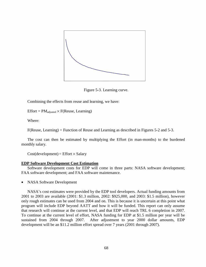
68

Figure 5-3. Learning curve.

Combining the effects from reuse and learning, we have:

Effort = PMadjusted × F(Reuse, Learning)

Where:

F(Reuse, Learning) = Function of Reuse and Learning as described in Figures 5-2 and 5-3.

The cost can then be estimated by multiplying the Effort (in man-months) to the burdened monthly salary.

Cost(development) = Effort × Salary

EDP Software Development Cost Estimation Software development costs for EDP will come in three parts: NASA software development;

FAA software development; and FAA software maintenance.

• NASA Software Development

NASA’s cost estimates were provided by the EDP tool developers. Actual funding amounts from 2001 to 2003 are available (2001: $1.3 million, 2002: $925,000, and 2003: $1.5 million), however only rough estimates can be used from 2004 and on. This is because it is uncertain at this point what program will include EDP beyond AATT and how it will be funded. This report can only assume that research will continue at the current level, and that EDP will reach TRL 6 completion in 2007. To continue at the current level of effort, NASA funding for EDP at $1.5 million per year will be sustained from 2004 through 2007. After adjustment to year 2000 dollar amounts, EDP development will be an $11.2 million effort spread over 7 years (2001 through 2007).

Learning Curve

Site Number

Relative Cost

Learning Curve

Site Number

Relative Cost

69

• FAA Software Development

We estimate FAA’s EDP software development effort in the same way as for McTMA (ref. 13). It is assumed that there will be as many FAA EDP spirals as there are deployment banks: one spiral for each deployment phase (see Section 3.3 for the assumed EDP deployment schedule). Three sets of reuse and learning factors were also selected based on our best judgment and values used in the McTMA LCCBA.

We assumed that code growth relative to each new site for EDP would be 10,000 SLOC (physical Source Lines Of Code), just as with McTMA. NASA’s EDP developers estimated that the EDP NASA baseline code size would probably be about 55,000 SLOC (roughly 17,185 logical Developed Source Instructions or DSI) more than FAA’s TMA Spiral 2 less the Dynamic Planner module which is not used by EDP. According to reference 13, FAA’s TMA Spiral 2 is estimated to be 736,350 SLOC, while the Dynamic Planner module is 46,988 SLOC. The inputs to COCOMO for calculating the FAA’s total software development costs (including cost factors such as software development, configuration management, and portions of software development Management and Administrative Support, or MAS costs) are listed in Table 5-2.

Table 5-2. FAA software development cost estimation inputs (14-site scenario).

SLOC DSI Reuse LearningNew Code 50,000 17,185 N/A N/ASpiral 1 Old Code 744,362 255,873 85% 100%New Code 40,000 13,748 N/A N/ASpiral 2 Old Code 794,362 273,061 100% 90%New Code 50,000 17,185 N/A N/ASpiral 3

Old Code 834,362 286,810 100% 90%Scale Drivers (SFi) 1.0775 Effort Multipliers (EMi) 1.3151 Labor Rate ($/month) 27,812

The total annual software development cost could then be calculated by adding the development cost of the new code (number of new sites multiplied by lines of new code in DSI each site) to a portion of the reengineering costs using COCOMO. The reengineering cost on the carried “old code” was assumed to spread evenly over the years of the corresponding deployment phase. Once this cost is obtained, the software development cost factor CDEV could be backed out using the factor F(DEV), derived from the software contractor’s Work Breakdown Structure (WBS, see ref. 13):

F(DEV) = (1 + %CM/%DEV) / (1 - %MAS_SW)

Where %CM, %DEV, and %MAS_SW denote percentage of efforts for Configuration Management, Development, and Software development portion of the MAS according to the WBS. The estimated EDP phase 1, 2, and 3 software development costs (corresponding to deployment banks 1, 2, and 3) for the 14-site scenario are $17.6, $2.5, and $2.9 million year 2000 dollars, respectively.

70

• FAA Software Maintenance (CMAI)

According to Table 5-2, the final EDP code count would be 884,362 SLOC (or 303,998 DSI) for the 14-site scenario. Based on TMA cost analysis, it is assumed that the first occurrence of software maintenance cost (the first year of the sustainment phase) sees a cost equivalent to 18% code change. Using the COCOMO equation without the factor of 1.07 to account for software development requirements, results in a cost of about $7.5 million for 2016. After that, an annual 3% decrease in cost applies until the end of Economic Service Life (ESL) of the last site.

CMAI = (1 – 3%)i-1 × $7,466,000

Where:

i is the ith year of the sustainment phase.

5.3.2. Hardware-Related Cost Estimation

As seen in Table 5-1, only three of the cost factors were estimated using a hardware cost-estimating model (first- and second-level repairs, hardware acquisitions, and software licenses). However, the costs could be substantial and should not be overlooked. The cost models for these cost factors are described in this section.

• Initial Hardware Acquisition (CIHW)

The initial hardware acquisition cost is a one-time cost at each site (TRACON). In discussions with NASA, it was determined that EDP would have hardware requirements that are very similar to TMA-Single Center. This assessment assumed that the initial hardware acquisition cost for each EDP deployment site would be the same as for TMA in FFP2, or $1 million per site. Thus:

CIHW = n × $1,000,000

Where:

n is the number of site installations for the year under consideration.

• Hardware Upgrades (CUHW)

According to the FAA, most of the commercial off-the-shelf (COTS) hardware used in a DST has an ESL of 6 years. For a 20-year life cycle, 3 hardware upgrades would be needed. However, the last upgrade would be very close to the end of life for EDP at a site. Therefore, we assumed that the intermittent EDP hardware equipment will be upgraded at the 7th and 14th year, with a per site upgrade cost of $615,000, as developed for TMA FFP1 cost profiles (ref. 13).

CUHW,i = mi × $615,000

Where:

71

mi is the total number of sites under EDP operation for year i.

• Annual Hardware Replacements (CAHW) and First- and Second-level Repairs (CRHW)

The observed TMA annual spare and repair rates (5.4% and 3% of the total hardware value) are assumed to be applicable to EDP (ref. 13).

CAHW = 5.4% × m × $1,000,000

CRHW = 3.0% × m × $1,000,000

• COTS Software Licenses (CASW)

And finally, it was assumed that EDP would have the same per-site annual COTS software license cost as TMA had in FFP1: roughly $15,000 (ref. 13).

CASW = m × $15,000

5.3.3. Other Cost Estimations

Most of the cost factors in Table 5-1 could only be assessed by other, ad hoc methods. We developed specialized cost estimating methodologies using either parametric, analogy, or expert judgment methods based on the analysis of TMA FFP1 and FFP2 costs. In most cases, CERs that had been developed from calibration of TMA cost data were adopted (ref. 13).

We believe many of the cost factors are proportional to size and complexity of the software code. Here, this report assumed the same scale of complexity for EDP as for TMA-SC. Thus, the ratio of the initial software code (or NASA baseline) was used as an adjustment factor when needed.

R(EDP/TMA) = Code Size (EDP NASA Baseline) / Code Size (TMA NASA Baseline)

• Technology Transfer

Among this group of cost factors, the main exception to the code size proportionality is the technology transfer cost. Our previous technology transfer cost estimate of approximately $1 million per year for two years (see ref. 1) was retained. The FAA’s TMA FFP1 cost profile captured only some reimbursement of travel costs for NASA employees and was deemed to be only a small portion of the total cost.

• MAS, ILS, Training Development, Systems Engineering, Configuration Management, Deployment, and Site Support of the Software Contractor

It was assumed that the EDP software contractor would use the same WBS structure as in TMA (ref. 13). The annual MAS cost, for example, can be calculated as:

CMAS_SW = CDEV × (%MAS_SW / %DEV)

72

Based on TMA cost analysis, we assumed that the total site support cost would be 10 times the contribution from the software contractor, and that it would be distributed evenly over time from the last year of software development’s level until the end of the program (ref. 13).

• MAS, Adaptation, Training Development, Systems Engineering, Configuration Management, and Deployment of the Adaptation Contractor

From the analyses of TMA cost information (ref. 13), we estimated the per-site total adaptation costs for TMA in FFP1 and FFP2 to be approximately $6.2 and $2.1 million, respectively (the difference being that the FFP1 adaptation costs included an “adaptation template” development cost). Following the same assessment method used for McTMA, it was assumed that the EDP per site adaptation cost would be that of TMA FFP2 adjusted by the factor of code size ratio, R(EDP/TMA). This makes the adaptation costs of the two DSTs roughly the same. Thus, we have the following formula:

Cost(adaptation) = p × $2,064,000 × R(EDP/TMA)

Where:

p is the number of sites adapted for that year.

The various adaptation cost factors can then be calculated using the WBS structure derived from TMA FFP2 (Table 3-16 in Section 3.4.2 of Ref. 13). For example:

CMAS_AD = Cost(adaptation) × %MAS_AD

The total deployment and configuration management costs are the sum of the costs from the software contractor and adaptation contractor.

• Site Implementation Planning

In reference 13, the TMA site implementation planning cost was derived at a little more than $1.4 million per site. Assuming that this planning cost is proportional to the code size, we have for EDP:

CSIP = p × $1,443,000 × R(EDP/TMA)

• Program Management Personnel (CPMP), Program Management Office (PMO) Support – Supplies & Travel (CPMO), and PM/Tech Support (CPMT)

Based on TMA FFP1 cost analysis results, the FAA applied 0.39 FTE of program management personnel at GSA grade 13.5 (annual cost of $120,000 per FTE) per million dollars of software and adaptation contracts during the deployment phase. This report assumes that this will be the case for EDP. Similarly, the TMA PMO support cost ratio of 34% is used to estimate EDP PMO support, consisting of supplies & travel costs (ref. 13).

73

CPMP = 0.39×$120,000× (Cost(adaptation) + Cost(development) × F(DEV) / %DEV)/1,000,000

CPMO = 0.34 × CPMP

We assume that these two cost factors will continue at the level of the last year of deployment through the end of the program (one year after the termination of the last site). All other program costs continue until termination of the last site.

The TMA annual PM/Tech Support FTE of 18.4 is adjusted by the ratio of code size and applies to the estimation of EDP PM/Tech support cost.

CPMT = 18.4 × $120,000 × R(EDP/TMA)

• Training and Training Support (CTTS)

It is assumed that the same level of effort used in training FAA personnel to operate TMA will be required for EDP: 3 FTEs per site at an hourly rate of $72.0 (ref. 13).

CTTS = ∑q 3.0 × $150,000

Where:

q is the number of sites under EDP operation for that year.

• Contract Award Process, IV&V, miscellaneous studies, functional integration, human integration, test plans, procedures, and reports, IOT&E, and performance measurement

During the McTMA LCC assessment, identical total miscellaneous studies, human integration, test plans, procedures, and reports, and performance measurement costs were assumed regardless of the sites deployed. Upon further consideration, it was decided that this group of cost factors should be related to the number of sites involved. The greater the number of deployment sites, the bigger the program. This would definitely require more effort and cost to be represented by these cost factors. Thus, these CERs are modified to reflect this functionality in the life cycle cost assessment of EDP. In additional to their direct relationship to the size of the software code, these CERs are assumed to be directly proportional to the ratio of the number of deployment sites between EDP and TMA (for TMA FFP1, there are 7 sites). Table 5-3 summarizes the per SLOC cost of each CER as observed during TMA FFP1.

Using contract award process as an illustrative example:

CCAP = Code Size(EDP NASA Baseline) × R(EDP sites/TMA sites) × $0.2

It is assumed that these costs will be evenly spread over their respective time frames. The calculated total performance measurement cost is distributed evenly within the deployment phase. During the sustainment phase, it is assumed that this cost is also proportional to the number of EDP sites in operation.

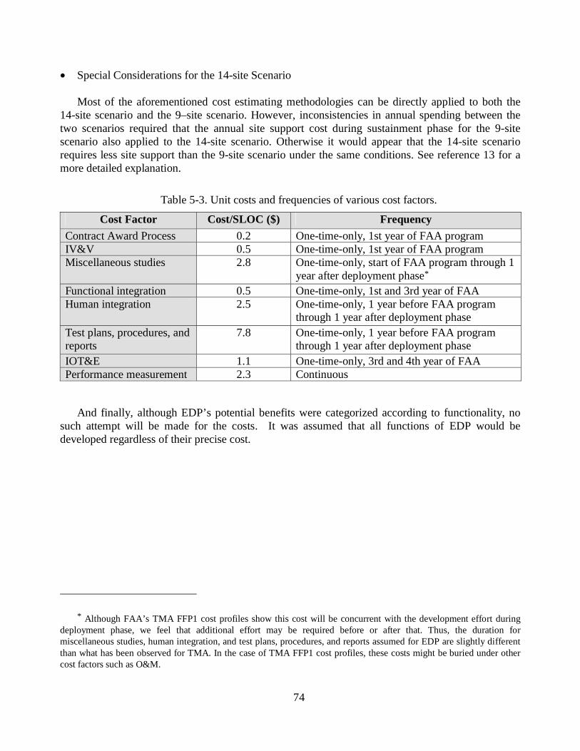
74

• Special Considerations for the 14-site Scenario

Most of the aforementioned cost estimating methodologies can be directly applied to both the 14-site scenario and the 9–site scenario. However, inconsistencies in annual spending between the two scenarios required that the annual site support cost during sustainment phase for the 9-site scenario also applied to the 14-site scenario. Otherwise it would appear that the 14-site scenario requires less site support than the 9-site scenario under the same conditions. See reference 13 for a more detailed explanation.

Table 5-3. Unit costs and frequencies of various cost factors.

Cost Factor Cost/SLOC ($) Frequency

Contract Award Process 0.2 One-time-only, 1st year of FAA programIV&V 0.5 One-time-only, 1st year of FAA programMiscellaneous studies 2.8 One-time-only, start of FAA program through 1

year after deployment phase*

Functional integration 0.5 One-time-only, 1st and 3rd year of FAA Human integration 2.5 One-time-only, 1 year before FAA program

through 1 year after deployment phase

Test plans, procedures, and reports

7.8 One-time-only, 1 year before FAA program through 1 year after deployment phase

IOT&E 1.1 One-time-only, 3rd and 4th year of FAA Performance measurement 2.3 Continuous

And finally, although EDP’s potential benefits were categorized according to functionality, no such attempt will be made for the costs. It was assumed that all functions of EDP would be developed regardless of their precise cost.

* Although FAA’s TMA FFP1 cost profiles show this cost will be concurrent with the development effort during deployment phase, we feel that additional effort may be required before or after that. Thus, the duration for miscellaneous studies, human integration, and test plans, procedures, and reports assumed for EDP are slightly different than what has been observed for TMA. In the case of TMA FFP1 cost profiles, these costs might be buried under other cost factors such as O&M.

75

6. EDP LCCBA RESULTS AND DISCUSSION

Two scenarios were studied for EDP LCCBA: a 14-site case (D10, N90, SCT, PCT, NCT, I90, C90, A80, MIA, D01, D21, M98, A90, and, PIT) and 9-site case (excluding the last 5 sites from the 14-site case). They were each evaluated over a 20-year ESL in accordance with FAA guidelines for various technologies (ref. 28). Using a 7% annual discount rate (ref. 19) and assuming the costs and benefits are uniformly spread throughout the year, the present value of the life-cycle costs and benefits were calculated according to the following formula:

[ ]5.0)1(1 −+×= nn iFVPV

Where: PV = Present Value

FVn = Future Value in the nth year

n = number (integer) of years from the base year (base year = 2000)

5.0)1(1 −+ ni is the mid-year discount factor, i = discount rate (7%)

6.1. EDP Life-Cycle Cost

The life cycle costs for the two cases considered are shown in Table 6-1.

Table 6-1. EDP life cycle cost results (Year 2000 $M).

Scenario Life-Cycle Cost

(Before Discounting) Life-Cycle Cost Present Value

(After Discounting) 14-site $417.3 $151.79-site $349.2 $135.6

Figures 6-1 and 6-2 depict the annual and cumulative costs before discounting. Figures 6-3 and 6-4 show the breakdown of the costs after discounting.

The before-discounting costs show a similar pattern. They start with the initial R&D costs, then show increasing implementation costs, then a leveling off, followed by generally decreasing costs with occasional peaks representing hardware refresh costs. The leveling off of the annual costs starts from year 2016 for the 14-site scenario when the project enters the sustainment phase (2013 for the 9-site scenario). This is because the annual costs during the DST sustainment years consist of annual maintenance, annual program management, and other recurring costs, with annual maintenance cost being the biggest contributor. We assumed that software maintenance would have an annual decreasing rate of 3%. At the end of their economic service lives, EDP installations are removed from service, beginning with the demonstration site. During this period, the annual cost decrease also reflects a reduced number of operational sites.

76

Figure 6-1. EDP annual and cumulative costs at 14 sites (before discounting).

Figure 6-2. EDP annual and cumulative costs at 9 sites (before discounting).

$0

$5

$10

$15

$20

$25

$30

$35

$40

$45

2002 2004 2006 2008 2010 2012 2014 2016 2018 2020 2022 2024 2026 2028 2030 2032 2034 2036

Year

An

nu

al

Co

sts

(Y

r20

00

$M

)

$0

$50

$100

$150

$200

$250

$300

$350

$400

$450

Cu

mu

lati

ve

Co

sts

(Y

r20

00

$M

)

Annual Costs

Cumulative Costs

$0

$5

$10

$15

$20

$25

$30

$35

$40

2001 2003 2005 2007 2009 2011 2013 2015 2017 2019 2021 2023 2025 2027 2029 2031 2033

Year

An

nu

al

Co

sts

(Y

r20

00

$M

)

$0

$50

$100

$150

$200

$250

$300

$350

$400

Cu

mu

lati

ve

Co

sts

(Y

r20

00

$M

)

Annual Costs

Cumulative Costs

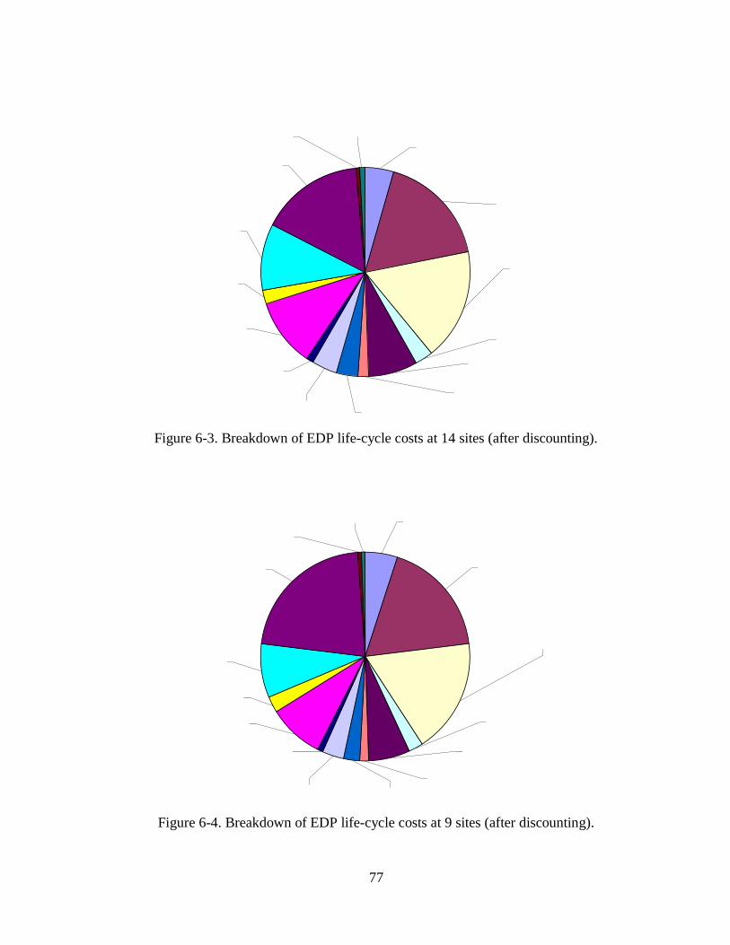
77

Figure 6-3. Breakdown of EDP life-cycle costs at 14 sites (after discounting).

Figure 6-4. Breakdown of EDP life-cycle costs at 9 sites (after discounting).

Software License0.7%IOT&E

0.6% NASA Development Costs4.3%

Software Maintenance16.1%

FAA Program Management17.5%

FAA Software Development17.4%

Adaptation2.8%

Systems Engineering7.3%

Integration1.8%

Hardware10.5%

In-Service management2.2%

Implementation10.5%

In-Service Support3.3%

Test and evaluation4.0%

Configuration Management1.0%

Software License0.6%

IOT&E0.4%

NASA Development Costs4.9%

Software Maintenance22.0%

FAA Program Management18.3%

FAA Software Development17.7%

Adaptation2.2%

Systems Engineering6.3%

Integration1.4%

Hardware8.4%

In-Service management2.3%

Implementation8.7%

In-Service Support2.6%

Test and evaluation3.2%

Configuration Management0.9%

78

6.2. EDP Life-Cycle Benefit

EDP life-cycle benefits are presented in Table 6-2, while Figures 6-5 and 6-6 show the annual and cumulative benefits before discounting for the EDP-Climb w/o SMS scenarios (these figures are representative). EDP-Climb w/o SMS represents the basic life-cycle benefits because it does not include indirect benefits due to integrated use with SMS. The annual benefits generally rise and fall with the number of sites in operation. When the number of sites remains constant, benefit continues to escalate. This is because benefits are proportional to annual operations, and annual operations increase linearly according to the FAA's terminal area forecast (ref. 11).

Table 6-2. EDP life-cycle benefit results (Year 2000 $M).

Scenario Life-Cycle Benefit

(Before Discounting) Life-Cycle Benefit Present Value

(After Discounting) EDP-Climb w/o SMS $1,078.5 $296.6EDP-Climb w/ SMS $1,530.6 $420.9EDP-Merge w/ SMS $1,654.8 $455.1

14-site

EDP-Both w/ SMS $3,158.4 $868.6

EDP-Climb w/o SMS $985.6 $277.6EDP-Climb w/ SMS $1,398.8 $394.1EDP-Merge w/ SMS $1,512.3 $426.0

9-site

EDP-Both w/ SMS $2,886.4 $813.1

Figure 6-5. EDP-Climb w/o SMS annual and cumulative benefits (14 sites, before discounting).

$0

$15

$30

$45

$60

$75

2002 2004 2006 2008 2010 2012 2014 2016 2018 2020 2022 2024 2026 2028 2030 2032 2034 2036

Year

An

nu

al B

en

efi

ts (

Yr2

000

$M

)

$0

$250

$500

$750

$1,000

$1,250

Cu

mu

lati

ve B

ene

fits

(Y

r20

00$M

)


Cumulative Benefits

79

Figure 6-6. EDP-Climb w/o SMS annual and cumulative benefits (9 sites, before discounting).

It should be noted that the economic benefit values represent airline direct operating cost savings, and do not include the savings in passenger value of time. The direct operating cost savings may not account for the full value of arrival and departure delay savings to airlines during rush periods, because this savings does not account for many operational implications, such as missed crew, passenger, baggage connections, etc, nor does it consider effects of abnormal operation conditions such as bad weather. Other possible potential benefits of EDP not included in this assessment include: reduced noise impact, and reduced emission. In other words this assessment could be conservative.

6.3. Life-Cycle Cost/Benefit Assessment

Table 6-3 summarizes the discounted costs, discounted benefits, benefit/cost ratios (B/C Ratio), Net Present Values (NPV), and Breakeven Points (BEP). Because we did not estimate EDP’s integration costs with SMS, only one LCC case each for the 14- and 9-site scenarios are assessed. Therefore, the LCCBA results for the “w/SMS” cases are of lower precision. The two “w/o SMS” cases are considered the “base case” results of this report. Note that a recent LCCBA of SMS (ref. 31) estimated generally higher potential benefits and B/C ratio for SMS than the values for EDP shown in Table 6-3. This makes the economic viability of both DSTs less vulnerable to integration costs.

The B/C ratios range from 1.96 to 5.73 for the 14-site scenarios and 2.05 to 6.00 for the 9-site scenarios. The above unity B/C ratios and positive NPV values indicate that benefits exceed costs for cases considered. The BEPs are 7, 5, 4, and 3 years after the PCA of the first site in 2008 for the

$0

$15

$30

$45

$60

$75

2001 2003 2005 2007 2009 2011 2013 2015 2017 2019 2021 2023 2025 2027 2029 2031 2033

Year

An

nu

al B

en

efi

ts (

Yr2

00

0$

M)

$0

$250

$500

$750

$1,000

$1,250

Cu

mu

lati

ve

Be

ne

fits

(Y

r20

00

$M

)


Cumulative Benefits

80

4 types of EDP benefits considered. Figures 6-7 and 6-8 are graphical representations of the discounted life-cycle costs and benefits for the 14- and 9-site scenarios, respectively.

Table 6-3. EDP life-cycle cost/benefit assessment results.

Scenario Discounted

Benefits (Year 2000 $M)

Discounted Costs

(Year 2000 $M) B/C

Ratio NPV

(Year 2000 $M) BEP EDP-Climb w/o SMS $296.6 1.96 $144.9 2015EDP-Climb w/ SMS $420.9 2.77 $269.2 2013EDP-Merge w/ SMS $455.1 3.00 $303.4 2012

14-site


$151.7

5.73 $716.9 2011


9-site


$135.6

6.00 $677.6 2011

Figure 6-7. EDP cumulative discounted life-cycle costs and benefits (14-site scenario).

$0

$100

$200

$300

$400

$500

$600

$700

$800

$900

2002 2004 2006 2008 2010 2012 2014 2016 2018 2020 2022 2024 2026 2028 2030 2032 2034 2036

Year

Ben

efit

s&C

ost

s ($

M, D

isco

un

ted

7%

/Yr)






81

Figure 6-8. EDP cumulative discounted life-cycle costs and benefits (9-site scenario).

6.4. Individual Site Life-Cycle Cost/Benefit Analysis

As described in Section 3.6, an added analysis for this study is “breaking-up” the EDP costs by the year 2000 normalized EDP Relative Potential Benefit ratios, as shown in Table 3-3, and comparing them to the life-cycle benefits for each site. This was suggested by NASA’s EDP developers as an indication of the site-by-site benefits and costs. This was done to all scenarios considered and we found that the results show certain commonality. A representative 14-site, EDP-Climb w/o SMS case is presented in Table 6-4 according to the site deployment order. The Benefit/Cost ratios of the 14 sites are plotted in Figure 6-9, with the dotted red line representing the overall B/C ratio.

Table 6-4. Individual site life-cycle cost/benefit results (14-site, EDP-Climb w/o SMS).

Site ID Life-Cycle Cost Present Value

(Year 2000 $M)

Life-Cycle Benefit Present Value

(Year 2000 $M)

NPV (Year 2000 $M)

B/C Ratio

D10 $3.8 $9.1 $5.3 2.37N90 $34.8 $71.7 $36.8 2.06SCT $33.0 $66.2 $33.2 2.01PCT $27.1 $53.2 $26.1 1.96NCT $17.7 $31.3 $13.5 1.76I90 $8.2 $15.6 $7.4 1.90C90 $7.9 $16.2 $8.3 2.04

$0

$100

$200

$300

$400

$500

$600

$700

$800

$900

2001 2003 2005 2007 2009 2011 2013 2015 2017 2019 2021 2023 2025 2027 2029 2031 2033

Year

Ben

efit

s&C

ost

s ($

M, D

isco

un

ted

7%

/Yr)






82

Table 6-4. (continued).

Site ID Life-Cycle Cost Present Value

(Year 2000 $M)

Life-Cycle Benefit Present Value

(Year 2000 $M)

NPV (Year 2000 $M)

B/C Ratio

A80 $4.0 $8.3 $4.3 2.06MIA $3.5 $6.1 $2.5 1.72D01 $2.5 $5.2 $2.7 2.10D21 $2.5 $4.5 $2.1 1.84M98 $2.3 $4.2 $1.9 1.81A90 $2.2 $2.5 $0.3 1.11PIT $2.0 $2.6 $0.6 1.30

14 sites $151.7 $296.6 $144.9 1.96

Figure 6-9. B/C ratios of the 14 sites individually for the EDP-Climb w/o SMS case.

The following can be said about Table 6-4 and Figure 6-9:

• The method used to distribute cost to each site slightly favors those with an earlier deployment schedule. This can be clearly seen in the case of D10.

• Excepting A90 and PIT, whose B/C ratios are low, all other sites have B/C ratio not too different from the overall case (represented by the dash line in the figure).

0.00

0.50

1.00

1.50

2.00

2.50


Site

B/C

Rat

io

B/C Ratios for individual sites

B/C Ratio for the overall case

83

• The ranking of sites decided by the 2000 RPB of EDP was not preserved. This was caused by the non-identical forecasted traffic growth rate at individual airports. The extreme cases are A90 and PIT, whose primary airports, BOS and PIT, have very low predicted traffic growth rates among the primary airports.

The discounted life-cycle benefits for each site in millions of year 2000 dollars are graphically shown in Figure 6-10.

Figure 6-10. EDP-Climb w/o SMS discounted life-cycle benefits of each site (year 2000 $M).

6.5. Discussion

The total EDP life cycle cost for the 9-site scenario is $135.6 million as estimated by this study. When compared with that of the 8-site scenario for McTMA, which was estimated at $208.0 million (see ref. 13, both LCCs are in year 2000 $ amounts), this estimate seems to be in-line with that of McTMA. Table 6-5 compares the major cost factors of EDP (both 9- and 14-site scenarios) and McTMA (8-site scenario), respectively. Note that the presumed negligible cost associated to the integration between EDP and SMS, necessary to the realization of ground savings, is not assessed.

PCT

A90N90

A80

MIA

D21PIT

M98

C90

D10

I90

x D01NCT

SCT $9.2

$72.7

$67.2

$54.0

$31.7

$15.9

$8.5

$6.2

$5.3

$4.6

$2.5

$2.6$16.4

$4.2

x

x

x

x

x

x

x

x

x

x

xx

x

PCT

A90N90

A80

MIA

D21PIT

M98

C90

D10

I90

x D01NCT

SCT $9.2

$72.7

$67.2

$54.0

$31.7

$15.9

$8.5

$6.2

$5.3

$4.6

$2.5

$2.6$16.4

$4.2

x

x

x

x

x

x

x

x

x

x

xx

x

84

Table 6-5. EDP and McTMA cost elements comparison (Year 2000 $M, discounted).

Cost Factors McTMA

8-site EDP 9-site

EDP 14-site

Software Maintenance $48.5 $29.5 $24.1FAA Program Management $39.1 $24.4 $26.3FAA Software Development $35.0 $23.7 $26.0Implementation $17.0 $11.7 $15.7Hardware $9.7 $11.2 $15.8Systems Engineering $13.5 $8.5 $10.9NASA Development Costs $14.0 $6.5 $6.5In-Service management $9.6 $5.0 $5.1Test and evaluation $5.1 $4.3 $6.1In-Service Support $5.7 $3.5 $4.9Adaptation $5.0 $3.0 $4.2Integration $1.9 $1.9 $2.7Configuration Management $1.9 $1.2 $1.5Software License $1.3 $0.8 $1.1IOT&E $0.7 $0.6 $0.9

Total $208.0 $135.6 $151.7

The highlighted entries in the McTMA column denote a reversal in rank when compared to the EDP 9-site case. McTMA had higher NASA development and software maintenance costs estimated because it was assumed by the McTMA developers that 200,000 lines of new code would be needed on top of the FAA’s TMA Spiral 2 (estimated at 736,350 SLOC; see ref. 13). Assumed EDP NASA baseline code size, on the other hand, is only a little more than that of FAA’s TMA Spiral 2 at 744,362 SLOC (see Section 0). Hence, NASA estimated that McTMA would have higher development cost than EDP.

Regarding our assessment of EDP’s potential benefits, one concern is the simulation of EDP’s precision spacing. This is a complicated issue concerning mainly, but not limited to, the time-step used in TAAM simulation. After adjusting settings such as in-trail separation, landing queue threshold, simulation time steps, etc., this study concluded that, if the desired change is equivalent to a change smaller than one simulation time-step (currently 6 seconds as in the FAA’s PCT simulation), TAAM could not produce consistent simulation results. However, because the FAA’s simulation model was run using the 6-second time-step and consistency with the FAA’s results was required, the values of certain settings (e.g., in-trail separation) were constrained. Given time, we would be able to re-baseline the model with a smaller time-step (the smallest currently available time step is 0.001 second, although the simulation speed suffers greatly), and produce a more extensive study on the effect of a smaller in-trail separation distance. A similar problem exists with TAAM’s conflict resolution. Based on our experiments, simulation results with enforcement of conflict resolution were not stable. Seemingly “minor” adjustments in some parameters often produced unbelievable outcomes, not unlike variation that occurs with different time steps. Furthermore, the combined effect of time-step settings and use of conflict resolution requires a lot more time to study. Thus, it was decided by the authors with the consensus of NASA’s EDP

85

engineers that this study would use the 6-second time step without enforcing conflict resolution in TAAM.

This decision helped us speed up the experimentation process and produce a set of TAAM parameters that yield reasonable results. Our a priori expectation was that the benefits from EDP’s merge advisory are in the form of reduced in-trail separation, resulting in reduced airborne time for departures. Contrary to our expectation, the simulation results show that reduced in-trail separation resulted only in reduced departure queue delay/taxi delay. The reduced departure queue delay/taxi delay is believed to be a direct result of a longer look-ahead time due to the “combination” of the Washington airports (i.e., better coordination between departure operations from separate airports).

On the arrival side, there are airborne savings on the faster jet arrivals. However, this is achieved by sacrifices taken by slower aircraft. Generally speaking, arrivals should not be affected greatly by departures. However, dual-use runways are a common occurrence at Washington airports, and we did not limit the ability of the arriving flight to switch runways at the same airport for landing during our simulations. Further study is required to fully understand this matter.

A sensitivity case was also studied where the major departure fixes were combined to create higher traffic “loading.” This is to simulate a situation where the in-trail separation in the Baseline is tighter, and hopefully generates more opportunities for EDP to improve the in-trail separation situation. With about 100% higher “load” at each “combined” fix, EDP simulation did not show the anticipated result, although more departure queue delay/taxi delay savings were observed. We suspect that at a location where even higher “loading” at the departure fixes caused delay in the air, EDP’s merging advisories would be able to reduce the in-trail separation and produce airborne time savings. However, this situation may be rare.

However, it was agreed by both the EDP developers and the authors that potential benefits due to EDP’s climb advisory is the primary benefit source. It should be noted again that a simulation tool like TAAM would not reproduce reality, and can only produce a simplified version of the reality to help air traffic analyses and studies. The time-average results are believed to be reliable. TAAM can be used to generate effects in the simulation on the same scale as in reality when certain parameters (operation conditions) are changed. We believe that this goal has been achieved in this study.

These results, however, raise an interesting question to the EDP developers. If the potential benefits from EDP’s merging advisory could only produce departure queue delay/taxi delay savings, which require simultaneous operation of a surface DST like SMS to materialize, perhaps the implementation of this particular function should be at a lower priority. We want to point out that although we believe these results, they might be inconclusive. More simulations need to be run, under different conditions, at other locations, coupled with other types of studies before a more definitive conclusion can be made. It would not hurt, though, to stage the implementation if possible so that the main, proven function of EDP—expedite climb profile—could receive undivided attention.

Recently, the Cost as an Independent Variable (CAIV) concept has gained popularity in Department of Defense and military acquisition programs. It is a process that helps to set performance objectives by performing cost-performance-schedule-risk trade-off studies. One such

86

trade-off could be performance (or potential benefit) increase and additional costs. As system performance and cost objectives are decided (on the basis of cost-performance-schedule-risk trade-offs), the requirements definition and acquisition processes will make cost more of a constraint, and less of a variable. This will nonetheless obtain the needed capability of the system, while reducing the Total Ownership Cost. In other words, it is important to identify where the “knee of the curve” is for the cost-performance-schedule-risk relationships and actively use this information in the design process. We feel, based on the results of this study, that a CAIV study of EDP is warranted.

87

7. SUMMARY

The primary objective of this report was to provide a life-cycle cost/benefit assessment (LCCBA) for EDP, an AATT computer-based analysis, prediction, and display Decision Support Tool for departure air traffic controllers.

In 2001, we performed a LCCBA study of 7 AATT DSTs, including EDP (ref. 1). However, new information regarding EDP and other, similar DSTs from various sources has enabled a more accurate LCCBA assessment. This required a revision of the LCCBA model, including the cost assessment methodology, and single-year benefit assessment, as well as benefit extrapolation methodology.

For the life cycle cost assessment, we adopted a cost assessment model calibrated with available TMA FFP1 and FFP2 cost data. This model was recently applied to a LCC assessment of McTMA, another DST in NASA’s CTAS tool suite, which was judged by the FAA Free Flight Program metrics team lead to be "at least in the ballpark” and “very realistic” (ref. 13). With minor modifications and improvements, this EDP study heavily leveraged the cost methodology used in the McTMA LCC assessment.

A fast-time simulation of air traffic at the Potomac TRACON, a possible EDP deployment site, was used to assess potential benefits of EDP. Unlike previous studies of EDP benefits, this approach addresses the operational issues and traffic flow at and around the study site. The benefit mechanisms quantified in this assessment are: expedited climb profiles, precision spacing, and improved departure queue.

To better understand EDP’s potential benefits, three simulations featuring various EDP functions were developed: 1) EDP’s climb advisories, 2) EDP’s merge advisories, and 3) both advisories. The simulation results were compared with a baseline derived from a simulation model of Potomac TRACON air traffic obtained from the FAA. The savings in time were then converted to economic benefits. The results show that EDP’s climb advisories function is the primary source of potential benefits. This agrees with EDP developer’s expectations. Airborne delay savings of a little less than 17 seconds per departure flight, and departure queue delay/taxi delay savings of a little under 2 seconds per departure flight, was achieved in simulation. EDP’s precision spacing advisory also seems to be able to generate significant savings (19 seconds per departure flight) for the departures on the ground, provided that a surface DST like SMS is operational at the site and proper linkage between the two tools is in effect. These EDP benefits were additive as demonstrated through simultaneous simulation of both EDP functions, i.e., a saving of 17 seconds in the air and 20 seconds on the ground per Washington departure flight.

Using a novel approach, EDP benefits at PCT were extrapolated to other sites and for other years. This benefits extrapolation methodology considered the combined effect of traffic growth and airspace complexity.

Using the site deployment model, this report evaluated two deployment scenarios of EDP: a 14-site scenario and a 9-site scenario. Three key economic metrics (net present value, benefit to cost

88

ratio, and breakeven point) were assessed. The life-cycle cost/benefit results were shown in the form of costs and benefits by year in year 2000 dollars. Life cycle cost characterization by cost elements was also presented. In addition, the total life cycle cost was appropriated to each EDP deployment site.

Although integrated use with SMS is assumed in order to assess potential EDP benefits due to reduction of departure queue delay/taxi delay, the costs associated with the integration effort are not estimated. Thus, the “w/SMS” LCCBA results should be viewed with this in mind.

The results show that potential benefits from implementing EDP for both the 14- and 9-site scenarios would be in excess of potential costs for every site. For the 14-site, EDP-Climb w/o SMS scenario, EDP would provide aviation users with direct benefits of $1.08 billion (before discounting) in constant 2000 dollars over its life cycle, while costing $417.3 million (before discounting). The cost-benefit translates to an NPV of $144.9 million, a B/C ratio of 1.96 and a breakeven point in the year 2015, 7 years after PCA of the first deployment site. Indirect benefits from cooperation of a surface DST like SMS increases the net present value to $269.2 million and improves the B/C ratio to 2.77, and moves the breakeven point 2 years earlier. For the 9-site scenario, the NPV and B/C ratio surpasses that of the 14-site scenario with the same breakeven point. This is because although less beneficial, the last few deployment sites require just about the same amount of deployment costs as the other sites. This can also be seen from their below-average B/C ratios when the total cost was distributed to each site using the same ratio of the benefit.

The most important cost factors in either scenario are software maintenance, FAA program management (including program management/technical support, management personnel, supplies and travel, miscellaneous studies, contract award process, and independent verification and validation costs), and FAA software development. Together these costs account for between 50 and 60 percent of the total life cycle cost after discounting. This result agrees with the assessed result of McTMA (ref. 13).

Although it was not a primary goal of this study to influence the technical aspects of the development of a DST, the results of this study suggest that more emphasis should be placed on developing and implementing the direct climb function of EDP. This is because it appears that benefits from implementing EDP’s merging advisory can only be realized through the integrated use of a surface DST if airborne departure capacity is not constrained. However, more extensive studies are needed on this subject to prove that this is universally true.

89

REFERENCES

1. Wang, Jianzhong; Barrington, Craig; and Datta, Koushik: Life Cycle Cost-Benefit Assessment of TMA, pFAST, EDP, SMA, SMS, aFAST, and McTMA. bd Systems Contract Report, Advanced Air Transportation Technologies Project, NASA Ames Research Center, Moffett Field, CA, Sept. 2001.

2. Suchkov, A.: Advanced Air Transportation Technologies RTO-48 Tasks 2 & 3 Report: Refined Benefits Assessment of Expedite Departure Path (EDP) Final Report. CSSI, Inc. Contract Report, Advanced Air Transportation Technologies Project, NASA Ames Research Center, Moffett Field, CA, 2001.

3. FAA: TMA FFP1 Cost Profiles. Spreadsheet and related information provided by the FAA. Free Flight Program Office, Federal Aviation Administration, Washington, D.C., May, 2002.

4. Lee, D., et al.: A Method for Making Cross-Comparable Estimates of the Benefits of Decision Support Technologies for Air Traffic Management. NASA/CR-1998-208455, LMI, 1998.

5. Couluris, G. J.; Weidner, T. J.: Terminal Airspace Decision Support Tool Functions Preliminary Potential Benefits Analysis. Seagull Contract Report, Advanced Air Transportation Technologies Project, NASA Ames Research Center, Moffett Field, CA, Dec. 1999.

6. Jung, Y. C.; and D. R. Isaacson: Design Concept and Development Plan of the Expedite Departure Path (EDP). AIAA Aircraft Technology, Integration, and Operations (ATIO) Conference, Los Angeles, CA, October 1-3, 2002.

7. Titan: AATT Operational Concept for ATM—Year 2002 Update. RTO-62 report from Titan Systems Corporation, Advanced Air Transportation Technologies Project, NASA Ames Research Center, Moffett Field, CA, Jan. 31, 2002.

8. NASA: Brief Expedite Departure Path Overview and Benefit Mechanisms. Internal report, Advanced Air Transportation Technologies Project, NASA Ames Research Center, Moffett Field, CA, Sept. 23, 2002.

9. NASA: Center TRACON Automation System (CTAS) – Expedite Departure Path. NASA Ames Research Center, Moffett Field, CA, April 2003. http://www.ctas.arc.nasa.gov/project_description/edp.html.

10. Datta, Koushik; Barrington, Craig; and Philip Reuter: An Initial Methodology to Categorize NAS Deployment of AATT Decision Support Tools. bd Systems Contract Report, Advanced Air Transportation Technologies Project, NASA Ames Research Center, Moffett Field, CA, Dec. 1999.

11. FAA: Terminal Area Forecast 2002. Federal Aviation Administration, Washington, D.C., 2002. http://www.apo.data.faa.gov/faatafall.htm.

90

12. AirNav, LLC: Airport Operational Statistics. AirNav, LLC, Morganville, NJ, 2002. http://www.airnav.com/airports/.

13. Wang, Jianzhong: Initial Life-Cycle Cost/Benefit Assessment of Multi-Center Traffic Management Advisor. bd Systems Contract Report, Advanced Air Transportation Technologies Project, NASA Ames Research Center, Moffett Field, CA, Aug. 30, 2002.

14. Wang, Jianzhong; and Datta, Koushik: A Life-Cycle Cost Estimating Methodology for NASA-Developed Air Traffic Control Decision Support Tools. NASA/CR-2002-211395, prepared for NASA Ames Research Center under Contract NAS2-98074, bd Systems, Inc., NASA Ames Research Center, Moffett Field, CA, Mar. 2002.

15. TPG: TAAM Plus, Fast Time Gate-to-Gate Simulation, Reference Manual. The Preston Group Pty Ltd., Richmond, Victoria 3121, Australia, 1999.

16. FAA: Economic Values for Evaluation of Federal Aviation Administration Investment and Regulatory Programs. FAA-APO-98-8, Office of Aviation Policy and Plans, Federal Aviation Administration, Washington, D.C., June 1998.

17. FAA: Air Traffic Control. FAA Order 7110.65M, Federal Aviation Administration, Washington, D.C., Feb. 2000.

18. Datta, Koushik; Karpe, Padma; and Barrington, Craig: Collaborative Departure Scheduling Benefit Assessment. Sverdrup Technology Contract Report. Advanced Air Transportation Technologies Project, NASA Ames Research Center, Moffett Field, CA, Dec. 1998.

19. OMB: Circular No. A-94, Revised Guidelines and Discount Rates for Benefit-Cost Analysis of Federal Programs. OMB Circular A-94, Office of Management and Budget, Oct. 1992.

20. FAA: Potomac Consolidated TRACON Airspace Study Report. Prepared by the Potomac Airspace Team, Federal Aviation Administration, Washington, D.C., Mar. 2001.

21. Wang, Jianzhong; Paul Chang; and Datta, Koushik: Refined Single-year Benefits Assessment of aFAST. Prepared for NASA Ames Research Center under Contract NAS2-98074, bd Systems, Inc., NASA Ames Research Center, Moffett Field, CA, Jan. 2003.

22. Barrington, Craig: Integrated Terminal and Surface Decision Support Benefit Assessment. Prepared for NASA Ames Research Center under Contract NAS2-98074, bd Systems, Inc., NASA Ames Research Center, Moffett Field, CA, Oct. 2000.

23. Boehm, Barry: Software Engineering Economics. Prentice Hall, Englewood Cliffs, NJ, 1981.

24. Center for Software Engineering, University of Southern California: COCOMO II Model Definition Manual. Updated Oct. 1998.

91

25. Center for Software Engineering, University of Southern California: USC COCOMO II Reference Manual. Updated Oct. 1998.

26. Selby, Richard W.; and Porter, Adam A.: Learning from examples – Generation and Evaluation of Decision Trees for Software Resource Analysis. IEEE Transactions on Software Engineering (ISSN 0098-5589), vol. 14, Dec. 1998, pp.1743–1757.

27. Management Concepts: Software Cost Estimating for NASA Ames Research Center. Course Handout, NASA Ames Research Center, Moffett Field, CA, Oct. 24–26, 2000.

28. FAA: FAA Acquisition System Toolset (FAST) – Investment Analysis Process. Office of Aviation Policy and Plans, Federal Aviation Administration, Washington, D.C., Sept. 2000. http://fast.faa.gov/.

29. FAA: Fixed Wing Aircraft Type Designators. Altoona Automated Flight Service Station, Federal Aviation Administration, Washington, D.C., Feb. 2000. http://www1.faa.gov/ats/afss/aooafss/plane/fixwing.htm.

30. Department of Labor: Consumer Price Index. Bureau of Labor Statistics, Department of Labor, Washington, D.C., Aug. 2003. http://data.bls.gov/cgi-bin/surveymost.

31. Raytheon Company: Advanced Air Transportation Technologies CTO-05 Task CTOD-5.15-2 Report: Initial Life-Cycle Benefits/Cost Assessment of Surface Management System (SMS). Contract Number NAS2-00015. Raytheon ATMSDI Team, Raytheon Company, 1001 Boston Post Road, Marlborough, MA 01752-3789, Oct. 2002.

REPORT DOCUMENTATION PAGEForm ApprovedOMB No. 0704-0188

Public reporting burden for this collection of information is estimated to average 1 hour per response, including the time for reviewing instructions, searching existing data sources, gatheringand maintaining the data needed, and completing and reviewing the collection of information. Send comments regarding this burden estimate or any other aspect of this collection ofinformation, including suggestions for reducing this burden, to Washington Headquarters Services, Directorate for Information Operations and Reports, 1215 Jefferson Davis Highway, Suite1204, Arlington, VA 22202-4302, and to the Office of Management and Budget, Paperwork Reduction Project (0704-0188), Washington, DC 20503.

1. AGENCY USE ONLY (Leave blank) 2. REPORT DATE02/2005

3. REPORT TYPE AND DATES COVEREDContractor Report

4. TITLE AND SUBTITLELife-Cycle Cost/Benefit Assessment of Expedite Departure Path (EDP)

5. FUNDING NUMBERSC-NAS2-98074

6. AUTHORSJianzhong Jay Wang, Paul Chang, Koushik Datta

7. PERFORMING ORGANIZATION NAME(S) AND ADDRESS(ES)bd Systems, Inc.Ames Research CenterMoffett Field, CA 94035

8. PERFORMING ORGANIZATIONREPORT NUMBER

A-0412745

9. SPONSORING/MONITORING AGENCY NAME(S) AND ADDRESS(ES)National Aeronautics and Space AdministrationWashington, DC 20546-0001

10. SPONSORING/MONITORING AGENCYREPORT NUMBER

NASA/CR–2005-212836

11. SUPPLEMENTARY NOTESPoint of Contact: Jianzhong Jay Wang, ASRC Aerospace Corp., Ames Research Center, M/S 210-15, Moffett Field, CA 94035(650) 604-3775

12a. DISTRIBUTION/AVAILABILITY STATEMENTUnclassified – UnlimitedSubject Category 03 Distribution: Non-StandardAvailability: NASA CASI (301)621-0390

12b. DISTRIBUTION CODE

13. ABSTRACT (Maximum 200 words)

This report presents a life-cycle cost/benefit assessment (LCCBA) of Expedite Departure Path (EDP)—an air traffic control DecisionSupport Tool (DST) currently under development at NASA. This assessment is an update of a previous study performed by bd Systems,Inc. (bd) during FY01, with the following revisions: The life-cycle cost assessment methodology developed by bd for the previous studywas refined and calibrated using Free Flight Phase 1 (FFP1) cost information for Traffic Management Advisor (TMA, or TMA-SC in theFAA’s terminology). Adjustments were also made to the site selection and deployment scheduling methodology to include airspacecomplexity as a factor. This technique was also applied to the benefit extrapolation methodology to better estimate potential benefits forother years, and at other sites. This study employed a new benefit estimating methodology because bd’s previous single year potentialbenefit assessment of EDP used unrealistic assumptions that resulted in optimistic estimates. This methodology uses an air trafficsimulation approach to reasonably predict the impacts from the implementation of EDP. The results of the costs and benefits analyseswere then integrated into a life-cycle cost/benefit assessment.

Presented results include annual costs and benefits, net present value, benefit-to-cost ratio, and break-even point. The results werebased on information available to bd Systems, Inc. at the time of this study.

15. NUMBER OF PAGES104

14. SUBJECT TERMSExpedite Departure Path (EDP), Life-Cycle Cost/Benefit Assessment (LCCBA), Life-Cycle Cost (LCC),Net Present Value, Benefit-to-Cost Ratio, Break-even point, Advanced Air TransportationTechnologies (AATT), Decision Support Tools (DSTs), Traffic Management Advisor (TMA), and TotalAirspace and Airport Modeller (TAAM)

16. PRICE CODE

17. SECURITY CLASSIFICATIONOF REPORT

Unclassified

18. SECURITY CLASSIFICATIONOF THIS PAGE

Unclassified

19. SECURITY CLASSIFICATIONOF ABSTRACT

Unclassified

20. LIMITATION OF ABSTRACT

Unclassified

NSN 7540-01-280-5500 Computer Generated STANDARD FORM 298 (Rev 2-89)Prescribed by ANSI Std 239-18

298-102

Life-Cycle Cost/Benefit Assessment of Expedite Departure ...

Documents

Transcript of Life-Cycle Cost/Benefit Assessment of Expedite Departure ...