Lecture 3 Regression Analysis
22
Prepared by Suwardo Regression Analysis Mathmatics and Statistics INTRODUCTION TO CHAPTER 11 REGRESSION ANALYSIS EGRESSION ANALYSIS NOTION SIMPLE LINEAR REGRESSION MODEL Model Estima ting Model Parameters Err or and Coefficient of Determination Prediction REGRESSION WITH TRANSFORMED V ARIABLES MULTIPLE LINEAR REGRESSION ANALYSIS Lecture 3
-
Upload
atina-tungga-dewi -
Category
Documents
-
view
235 -
download
0
Transcript of Lecture 3 Regression Analysis
7/28/2019 Lecture 3 Regression Analysis
http://slidepdf.com/reader/full/lecture-3-regression-analysis 1/22
Prepared by SuwardoRegression Analysis
Mathmatics and Statistics
INTRODUCTION TO CHAPTER 11
REGRESSION ANALYSISEGRESSION ANALYSIS
NOTION
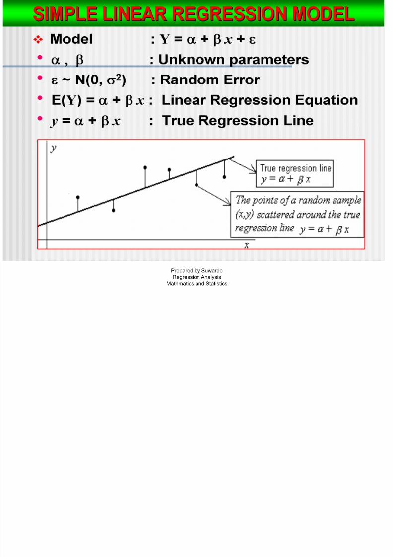
SIMPLE LINEAR REGRESSION MODEL
Model
Estimating Model Parameters
Error and Coefficient of Determination
Prediction
REGRESSION WITH TRANSFORMED VARIABLES
MULTIPLE LINEAR REGRESSION ANALYSIS
Lecture 3
7/28/2019 Lecture 3 Regression Analysis
http://slidepdf.com/reader/full/lecture-3-regression-analysis 2/22
Prepared by SuwardoRegression Analysis
Mathmatics and Statistics
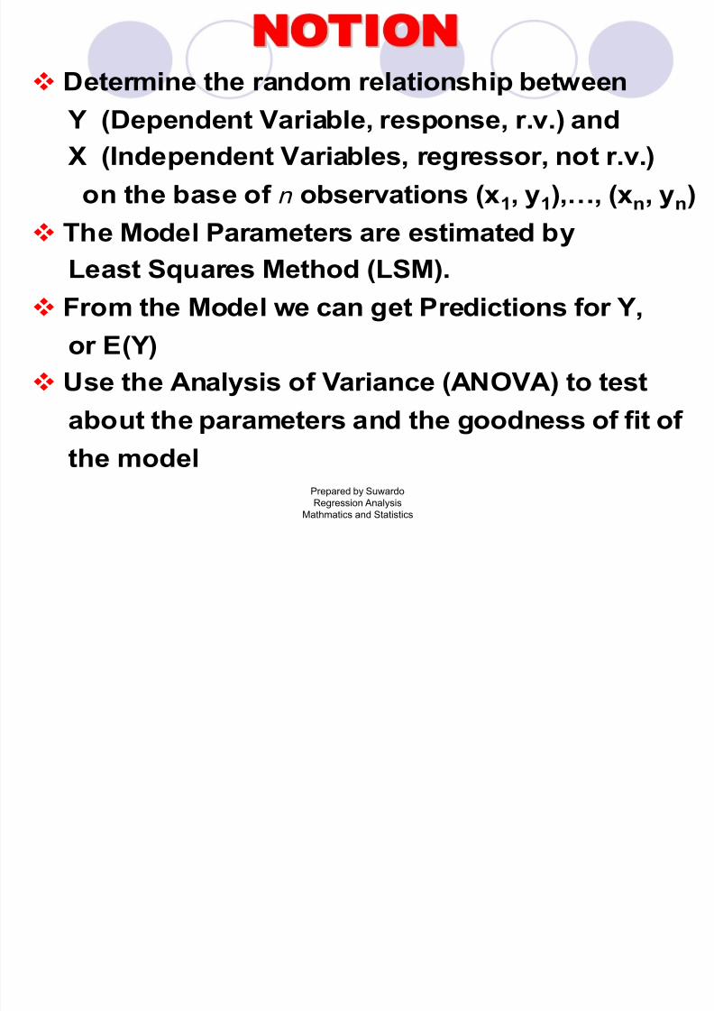
NOTIONOTION Determine the random relationship between
Y (Dependent Variable, response, r.v.) andX (Independent Variables, regressor, not r.v.)
on the base of n observations (x1, y1),…, (xn, yn)
The Model Parameters are estimated by
Least Squares Method (LSM).
From the Model we can get Predictions for Y,
or E(Y)
Use the Analysis of Variance (ANOVA) to test
about the parameters and the goodness of fit of
the model
7/28/2019 Lecture 3 Regression Analysis
http://slidepdf.com/reader/full/lecture-3-regression-analysis 3/22
Prepared by SuwardoRegression Analysis
Mathmatics and Statistics
7/28/2019 Lecture 3 Regression Analysis
http://slidepdf.com/reader/full/lecture-3-regression-analysis 4/22

7/28/2019 Lecture 3 Regression Analysis
http://slidepdf.com/reader/full/lecture-3-regression-analysis 5/22
Prepared by SuwardoRegression Analysis
Mathmatics and Statistics
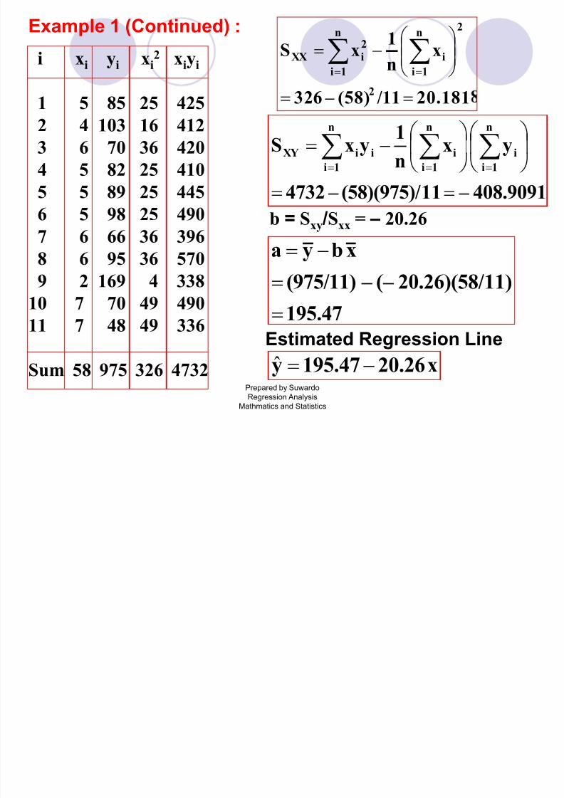
ESTIMATING MODEL PARAMETERSSTIMATING MODEL PARAMETERS
Using the Least Squares Method, are estimated
by a, b, and we get , the Estimated
Regression Line
bxay ˆ
n
1i
i
n
1i
i
n
1i
i
n
1i
iixy
n
1i
i
2n
1i
i
n
1i
2
ixx
xx
xy
n
1i
2
ii
2
i
n
1i
i
yn
1y,yx
n
1)y(xS
x
n
1x,x
n
1)(xS
where,xbyaand,SSbThen
min!)bxa(y)y(ySSE ˆ
7/28/2019 Lecture 3 Regression Analysis
http://slidepdf.com/reader/full/lecture-3-regression-analysis 6/22
7/28/2019 Lecture 3 Regression Analysis
http://slidepdf.com/reader/full/lecture-3-regression-analysis 7/22
Prepared by SuwardoRegression Analysis
Mathmatics and Statistics
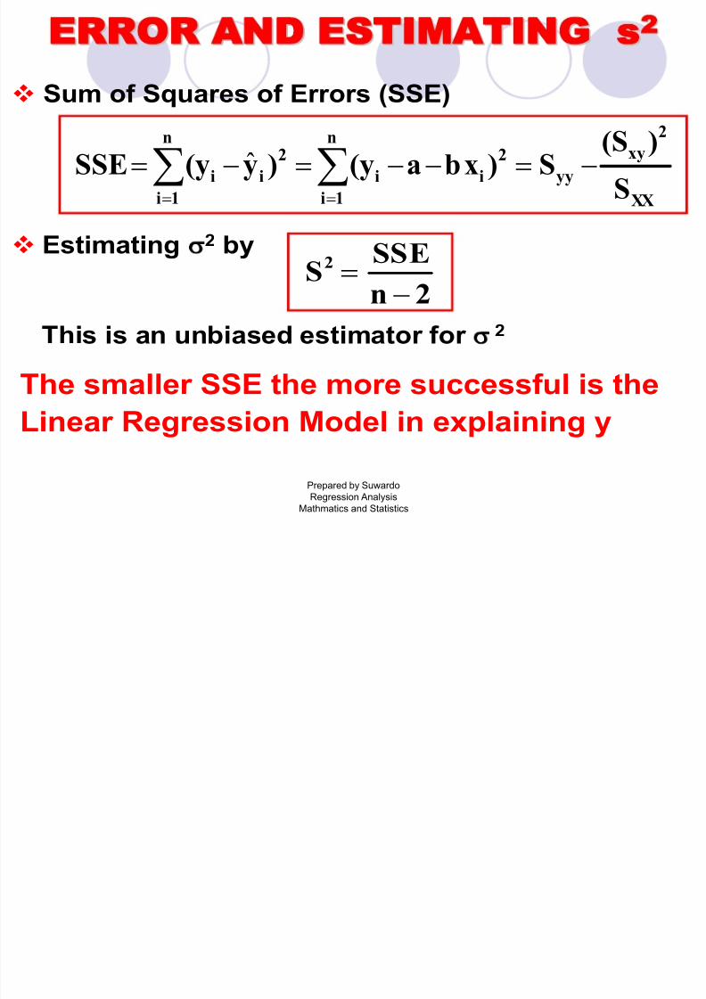
ERROR AND ESTIMATING sRROR AND ESTIMATING s2
Sum of Squares of Errors (SSE)
Estimating 2 by
This is an unbiased estimator for 2
The smaller SSE the more successful is the
Linear Regression Model in explaining y
XX
2
xy
yy
n
1i
2
ii
2
i
n
1i
iS
)(SS)xba(y)y(ySSE
ˆ
2n
SSES2
7/28/2019 Lecture 3 Regression Analysis
http://slidepdf.com/reader/full/lecture-3-regression-analysis 8/22
Prepared by SuwardoRegression Analysis
Mathmatics and Statistics
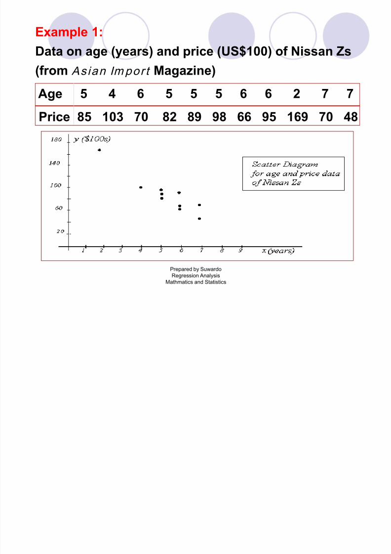
Example 1 (Continued) :
1 5 85 25 425
2 4 103 16 412
3 6 70 36 420
4 5 82 25 410
5 5 89 25 445
6 5 98 25 4907 6 66 36 396
8 6 95 36 570
9 2 169 4 338
10 7 70 49 49011 7 48 49 336
Sum 58 975 326 4732
94.16 83.9
114.42 130.5
73.90 15.2
94.16 147.9
94.16 26.6
94.16 14.773.90 62.4
73.90 445.2
154.95 197.5
53.64 267.753.64 31.8
iy2
ii )yy(
1423.5
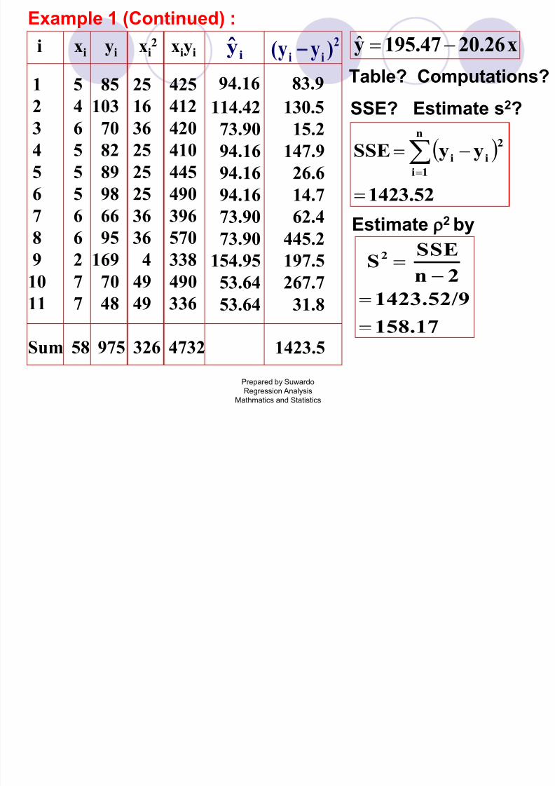
x20.26195.47y ˆ
Table? Computations?
SSE? Estimate s2?
1423.52
yySSEn
1i
2
ii
ˆ
Estimate 2 by
158.17
1423.52/9
2n
SSES
2
i xi yi xi2 xiyi
7/28/2019 Lecture 3 Regression Analysis
http://slidepdf.com/reader/full/lecture-3-regression-analysis 9/22
Prepared by SuwardoRegression Analysis
Mathmatics and Statistics
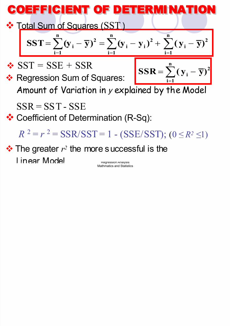
COEFFICIENT OF DETERMINATIONOEFFICIENT OF DETERMI NATION
Coefficient of Determination (R-Sq):
R 2 = r 2 = SSR/SST = 1 - (SSE/SST); (0 ≤ R2 ≤1)
The greater r 2 the more successful is the
2i
n
1i
2i
n
1i
i2
n
1i
i )yy()y(y)y(ySST
ˆˆ
2n
1i
i )yy(SSR
ˆ
Total Sum of Squares (SST )
SST = SSE + SSR
Regression Sum of Squares:Amount of Variation in y explained by the Model
SSR = SST - SSE
7/28/2019 Lecture 3 Regression Analysis
http://slidepdf.com/reader/full/lecture-3-regression-analysis 10/22
Prepared by SuwardoRegression Analysis
Mathmatics and Statistics
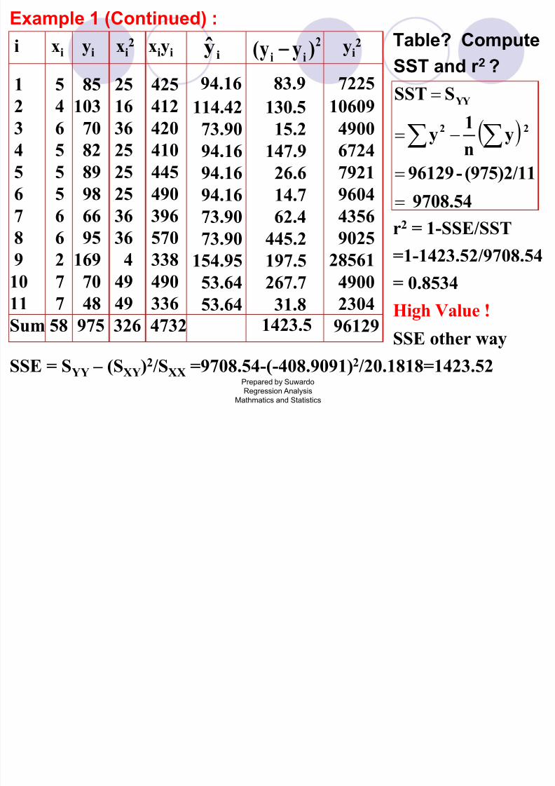
Example 1 (Continued) :
1 5 85 25 425
2 4 103 16 412
3 6 70 36 420
4 5 82 25 410
5 5 89 25 445
6 5 98 25 4907 6 66 36 396
8 6 95 36 570
9 2 169 4 338
10 7 70 49 49011 7 48 49 336
Sum 58 975 326 4732
94.16 83.9
114.42 130.5
73.90 15.2
94.16 147.9
94.16 26.6
94.16 14.773.90 62.4
73.90 445.2
154.95 197.5
53.64 267.753.64 31.8
iy2
ii )yy(
1423.5
7225
10609
4900
6724
7921
96044356
9025
28561
49002304
96129
yi2 i xi yi xi
2 xiyiTable? Compute
SST and r 2 ?
9708.54
(975)2/11-96129
yn
1y
SSST
22
YY
r2 = 1-SSE/SST
=1-1423.52/9708.54
= 0.8534High Value !
SSE = SYY – (SXY)2/SXX =9708.54-(-408.9091)2/20.1818=1423.52
SSE other way

7/28/2019 Lecture 3 Regression Analysis
http://slidepdf.com/reader/full/lecture-3-regression-analysis 11/22
Prepared by SuwardoRegression Analysis
Mathmatics and Statistics
Confidence Interval on the Slope
A 100(1-α)% CI for the parameter β in the linear regression is
xxn
S st
bb
/ where 2,2/
Hypothesis Testing on the Significance of Regression (on
the Slope)
Test the hypothesis
H0 : β = 0 ( there is no relationship between x and Y)
H1: β ≠ 0 (the straight-line model is adequate)
Test Statistic: T – distribution.
Critical Region: |T | > tα/2, n-2 . xxS S
bT
/
7/28/2019 Lecture 3 Regression Analysis
http://slidepdf.com/reader/full/lecture-3-regression-analysis 12/22
Prepared by SuwardoRegression Analysis
Mathmatics and Statistics
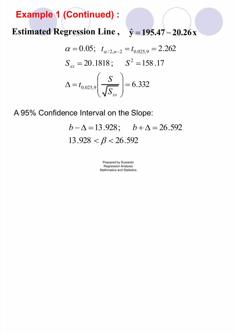
Example 1 (Continued) :
x20.26195.47y ˆ
332.6
17.158;1818.20
262.2;05.0
9,025.0
2
9,025.02,2/
xx
xx
n
S
S t
S S
t t
Estimated Regression Line ,
A 95% Confidence Interval on the Slope:
592.26928.13
592.26;928.13
bb
7/28/2019 Lecture 3 Regression Analysis
http://slidepdf.com/reader/full/lecture-3-regression-analysis 13/22
Prepared by SuwardoRegression Analysis
Mathmatics and Statistics
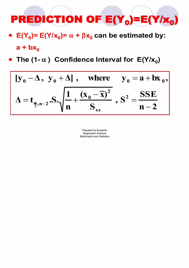
PREDICTION OF E(Y0)=E(Y/x0)
E(Y0)= E(Y/x0)= + x0 can be estimated by:
a + bx0
The (1- ) Confidence Interval for E(Y/x0)
2n
SSES,
S
)x(x
n
1.S.tΔ
,bxaywhere,Δ]y,Δy[
2
xx
2
02n,
0000
2α
ˆˆˆ
7/28/2019 Lecture 3 Regression Analysis
http://slidepdf.com/reader/full/lecture-3-regression-analysis 14/22
Prepared by Suwardo
Regression Analysis
Mathmatics and Statistics
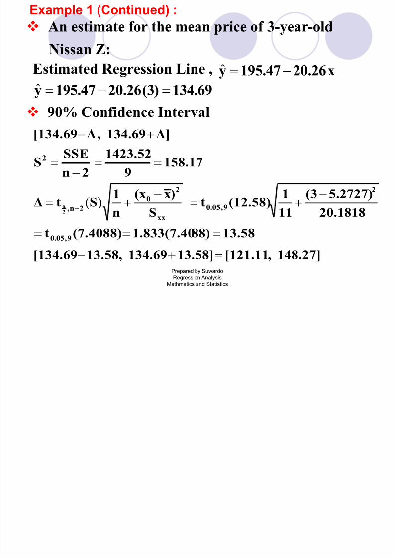
An estimate for the mean price of 3-year-old
Nissan Z:
Estimated Regression Line , x20.26195.47y ˆ134.69(3)20.26195.47y ˆ
90% Confidence Interval
148.27],[121.1113.58]134.69,13.58[134.69
13.5888)1.833(7.40(7.4088)t
20.1818
5.2727)(3
11
1
(12.58)tS
)x(x
n
1
StΔ
158.179
1423.52
2n
SSES
Δ]134.69,Δ[134.69
9,0.05
2
9,0.05
xx
2
0
2n,
2
2α
)(
Example 1 (Continued) :
7/28/2019 Lecture 3 Regression Analysis
http://slidepdf.com/reader/full/lecture-3-regression-analysis 15/22
Prepared by Suwardo
Regression Analysis
Mathmatics and Statistics
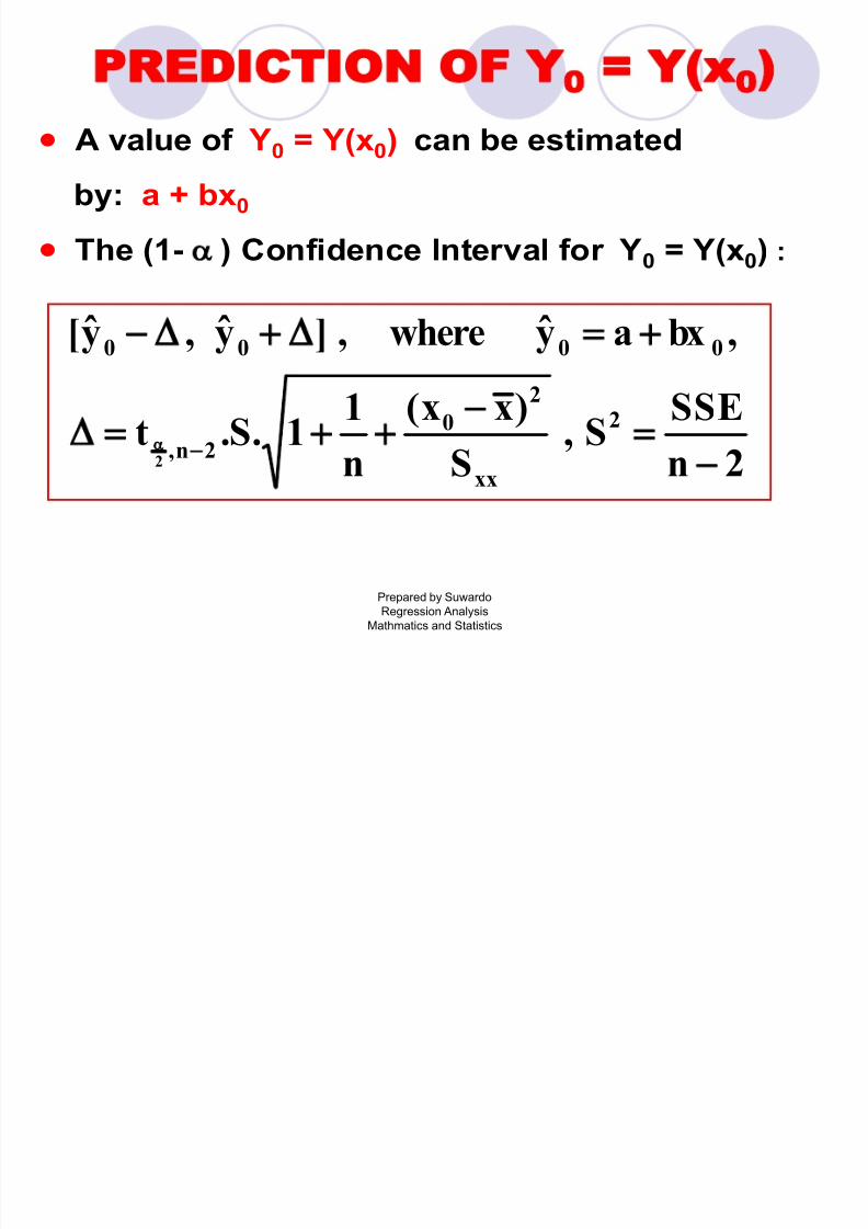
PREDICTION OF Y0 = Y(x0)
A value of Y0 = Y(x0) can be estimatedby: a + bx0
The (1- ) Confidence Interval for Y0 = Y(x0) :
2n
SSE
S,S
)xx(
n
1
1.S.t
,bxaywhere,]y,y[
2
xx
2
0
2n,
0000
2

7/28/2019 Lecture 3 Regression Analysis
http://slidepdf.com/reader/full/lecture-3-regression-analysis 16/22
Prepared by Suwardo
Regression Analysis
Mathmatics and Statistics
An estimate for the price of 3-year-old Nissan Z:
Estimated Regression Line , x20.26195.47y ˆ
134.69(3)20.26195.47y ˆ
90% Confidence Interval
161.45],[107.9326.76]134.69,26.76[134.69
26.76995)1.833(14.5(14.5995)t
20.1818
5.2727)(3
11
11(12.58)tS
)x(x
n
11StΔ
158.179
1423.52
2n
SSES
Δ]134.69,Δ[134.69
9,0.05
2
9,0.05
xx
2
0
2n,
2
2α
)(
Example 1 (Continued) :
7/28/2019 Lecture 3 Regression Analysis
http://slidepdf.com/reader/full/lecture-3-regression-analysis 17/22
7/28/2019 Lecture 3 Regression Analysis
http://slidepdf.com/reader/full/lecture-3-regression-analysis 18/22
Prepared by Suwardo
Regression Analysis
Mathmatics and Statistics
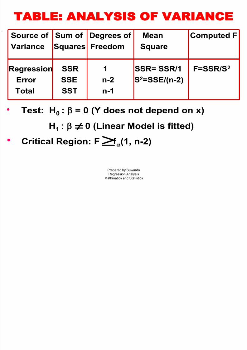
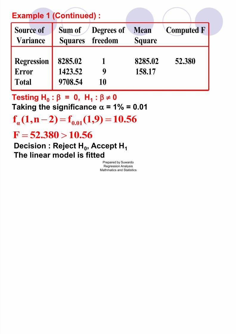
Source of Sum of Degrees of Mean Computed F
Variance Squares freedom Square
Regression 8285.02 1 8285.02 52.380
Error 1423.52 9 158.17
Total 9708.54 10
Example 1 (Continued) :
Testing H0 : = 0, H1 : 0
Taking the significance = 1% = 0.01
10.5652.380F10.56(1,9)f 2)n(1,f 0.01α
Decision : Reject H0, Accept H1 The linear model is fitted

7/28/2019 Lecture 3 Regression Analysis
http://slidepdf.com/reader/full/lecture-3-regression-analysis 19/22
Prepared by Suwardo
Regression Analysis
Mathmatics and Statistics
The regression equation is price = 195 - 20.3 age
Predictor Coef SE Coef T P
Constant 195.47 15.24 12.83 0.000
age -20.261 2.800 -7.24 0.000
S = 12.58 R-Sq = 85.3%
Analysis of Variance
Source DF SS MS F PRegression 1 8285.0 8285.0 52.38 0.000
Residual Error 9 1423.5 158.2
Total 10 9708.5
Statistical output from Minitab
7/28/2019 Lecture 3 Regression Analysis
http://slidepdf.com/reader/full/lecture-3-regression-analysis 20/22
Prepared by Suwardo
Regression Analysis
Mathmatics and Statistics
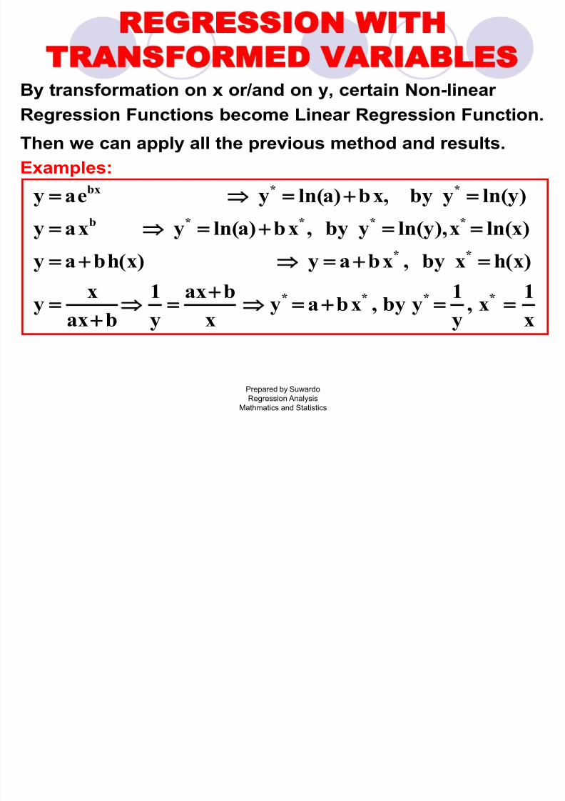
REGRESSION WITH
TRANSFORMED VARIABLESBy transformation on x or/and on y, certain Non-linear
Regression Functions become Linear Regression Function.
Then we can apply all the previous method and results.
x1x,
y1yby,xbay
xbax
y1
baxxy
)x(hxby,xbay)x(hbay
)xln(x),yln(yby,xb)aln(yxay
)yln(yby,xb)aln(yeay
****
**
****b
**bx
Examples:

7/28/2019 Lecture 3 Regression Analysis
http://slidepdf.com/reader/full/lecture-3-regression-analysis 21/22

7/28/2019 Lecture 3 Regression Analysis
http://slidepdf.com/reader/full/lecture-3-regression-analysis 22/22
Prepared by Suwardo
Regression Analysis
Mathmatics and Statistics
SUMMARY OF CHAPTER 11
REGRESSION ANALYSISEGRESSION ANALYSIS
NOTION
SIMPLE LINEAR REGRESSION MODEL
Model
Estimating Model Parameters
Error and Coefficient of Determination
Prediction
REGRESSION WITH TRANSFORMED VARIABLES MULTIPLE LINEAR REGRESSION ANALYSIS