MATH 3P82REGRESSION ANALYSIS

Lecture Notes

c° Jan Vrbik

2

3

Contents

1 PREVIEW 5

2 USING MAPLE 7Basics . . . . . . . . . . . . . . . . . . . . . . . . . . . . . . . . . . . . . 7Lists and Loops . . . . . . . . . . . . . . . . . . . . . . . . . . . . . . . . 8Variables and Polynomials . . . . . . . . . . . . . . . . . . . . . . . . . . 9Procedures . . . . . . . . . . . . . . . . . . . . . . . . . . . . . . . . . . 10Matrix Algebra . . . . . . . . . . . . . . . . . . . . . . . . . . . . . . . . 10

Other useful commands: . . . . . . . . . . . . . . . . . . . . . . . . 11Plots . . . . . . . . . . . . . . . . . . . . . . . . . . . . . . . . . . . . . . 11

3 SIMPLE REGRESSION 13Maximum Likelihood Method . . . . . . . . . . . . . . . . . . . . . . . . 13Least-Squares Technique . . . . . . . . . . . . . . . . . . . . . . . . . . . 13

Normal equations . . . . . . . . . . . . . . . . . . . . . . . . . . . . 14Statistical Properties of the three Estimators . . . . . . . . . . . . . . . . 15Confidence Intervals . . . . . . . . . . . . . . . . . . . . . . . . . . . . . 17

Regression coefficients . . . . . . . . . . . . . . . . . . . . . . . . . 18Residual variance . . . . . . . . . . . . . . . . . . . . . . . . . . . . 18Expected-value estimator . . . . . . . . . . . . . . . . . . . . . . . . 19New y value . . . . . . . . . . . . . . . . . . . . . . . . . . . . . . . 19

Hypotheses Testing . . . . . . . . . . . . . . . . . . . . . . . . . . . . . . 20Model Adequacy (Lack-of-Fit Test) . . . . . . . . . . . . . . . . . . . . . 20Weighted Regression . . . . . . . . . . . . . . . . . . . . . . . . . . . . . 22Correlation . . . . . . . . . . . . . . . . . . . . . . . . . . . . . . . . . . 24Large -Sample Theory . . . . . . . . . . . . . . . . . . . . . . . . . . . . 26

Confidence interval for the correlation coefficient . . . . . . . . . . . 27

4 MULTIVARIATE (LINEAR) REGRESSION 29Multivariate Normal Distribution . . . . . . . . . . . . . . . . . . . . . . 29

Partial correlation coefficient . . . . . . . . . . . . . . . . . . . . . . 30Multiple Regression - Main Results . . . . . . . . . . . . . . . . . . . . . 31

Various standard errors . . . . . . . . . . . . . . . . . . . . . . . . . 33Weighted-case modifications . . . . . . . . . . . . . . . . . . . . . . 34

Redundancy Test . . . . . . . . . . . . . . . . . . . . . . . . . . . . . . . 35Searching for Optimal Model . . . . . . . . . . . . . . . . . . . . . . . . 37Coefficient of Correlation (Determination) . . . . . . . . . . . . . . . . . 38

4

Polynomial Regression . . . . . . . . . . . . . . . . . . . . . . . . . . . . 39Dummy (Indicator) Variables . . . . . . . . . . . . . . . . . . . . . . . . 40Linear Versus Nonlinear Models . . . . . . . . . . . . . . . . . . . . . . . 42

5 NONLINEAR REGRESSION 43

6 ROBUST REGRESSION 47Laplace distribution . . . . . . . . . . . . . . . . . . . . . . . . . . . . . 47Cauchy Case . . . . . . . . . . . . . . . . . . . . . . . . . . . . . . . . . 50

7 TIME SERIES 53Markov Model . . . . . . . . . . . . . . . . . . . . . . . . . . . . . . . . . 53Yule Model . . . . . . . . . . . . . . . . . . . . . . . . . . . . . . . . . . 55

5

Chapter 1 PREVIEWRegression is a procedure which selects, from a certain class of functions, the onewhich best fits a given set of empirical data (usually presented as a table of x and yvalues with, inevitably, some random component). The ’independent’ variable x isusually called the regressor (there may be one or more of these), the ’dependent’variable y is the response variable.. The random components (called residuals)are usually assumed normally distributed, with the same σ and independent of eachother.The class from which the functions are selected (the model) is usually one of

the following types:

1. a linear function of x (i.e. y = a+ b x) - simple (univariate) linear regression,

2. a linear function of x1, x2, ... xk - multiple (multivariate) linear regression,

3. a polynomial function of x - polynomial regression,

4. any other type of function, with one or more parameters (e.g. y = a ebx) -nonlinear regression.

The coefficients (parameters) of these models are called regression coeffi-cients (parameters). Our main task is going to be to find good estimators ofthe regression coefficients (they should have correct expected values and variancesas small as possible), to be used for predicting values of y when new observationsare taken.Some of the related issues are:

1. How do know (can we test) whether the relationship (between y and x)is truly linear? What if it is not (we have switch to either polynomial ornonlinear model).

2. Similarly, are the residuals truly normal and independent of each other? Howdo we fix the procedure if the answer is NO.

3. Even when they are normal and independent, what if their variance changeswith x (here, we have to do the so called weighted regression).

4. Even when all the assumptions are properly met: In the multivariate casewith many independent variables, do we really need them all to make a goodprediction about y ? And, if it is possible to reduce them (usually substan-tially) to a smaller subset, how do we do it (i.e. selecting the best five,say).?

6

7

Chapter 2 USING MAPLEBasicsTyping an expression (following Maple’s > prompt) results in evaluating it.When the expression contains only integers (no decimal point), one gets the exact(rational) answer, as soon as at least one number in the expression is real (with adecimal point), the result is real (rounded off to 10 significant digits). The symbols∗, / and ˆ facilitate multiplication, division and exponentiation, respectively. Notethat each line of your input has to end with a semicolon:

> 4 ∗ 5− 3 / (5 + 2) + 2 ˆ (−3) ;110356

The result of any computation can be stored under a name (which you make up,rather arbitrarily), and used in any subsequent expression. Maple then remembersthe value, until the end of your session, or till you deliberately replace it with anew value. Note that this (giving a name to a result) is achieved by typing thename, followed by a colon and the equal sign (a group of two symbols, representinga single operation), followed by the actual expression to be stored:

> a := (3.0 + 4) ∗ (2− 6) + 2 / 3− 4 / 5 ;a := −28. 13333 333

> a/ 7 + 9 ;

4. 98095 238

> a := 14 / 6 ;

a := 73;

> a/ 7 + 9 ;

a := 283;

(from now on, we will omit the > prompt from our examples, showing onlywhat we have to type).Maple can also handle the usual functions such as sin, cos, tan, arcsin,

arccos, arctan, exp, ln, sqrt, etc. All angles are always measured in radians.

sin(3.) ; sqrt(8) ;

.14112 00081

2√2

We can also define our own functions by:

f := x− > x ˆ 2 ;

8

f := x→ x2

f(3);

9

where f is an arbitrary name.

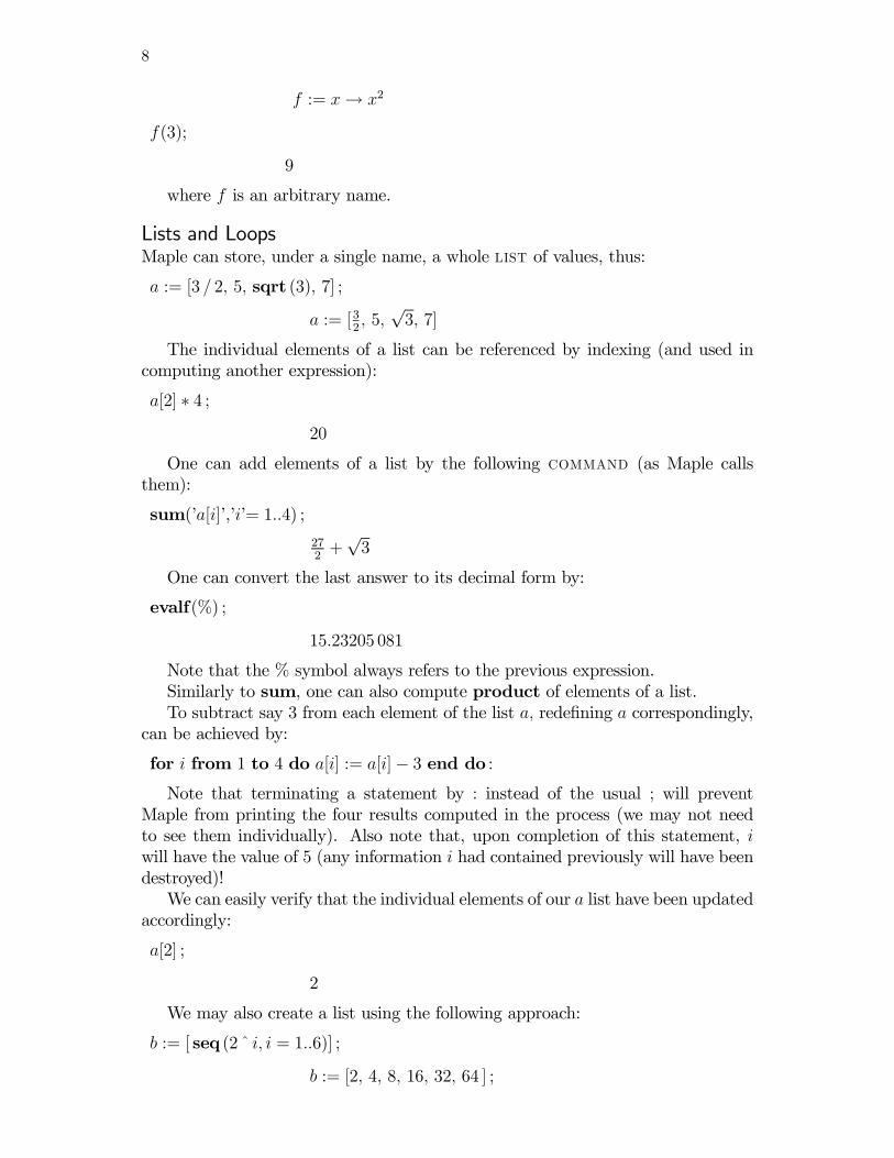
Lists and LoopsMaple can store, under a single name, a whole list of values, thus:

a := [3 / 2, 5, sqrt (3), 7] ;

a := [32, 5,√3, 7]

The individual elements of a list can be referenced by indexing (and used incomputing another expression):

a[2] ∗ 4 ;20

One can add elements of a list by the following command (as Maple callsthem):

sum(’a[i]’,’i’= 1..4) ;272+√3

One can convert the last answer to its decimal form by:

evalf(%) ;

15.23205 081

Note that the % symbol always refers to the previous expression.Similarly to sum, one can also compute product of elements of a list.To subtract say 3 from each element of the list a, redefining a correspondingly,

can be achieved by:

for i from 1 to 4 do a[i] := a[i]− 3 end do :Note that terminating a statement by : instead of the usual ; will prevent

Maple from printing the four results computed in the process (we may not needto see them individually). Also note that, upon completion of this statement, iwill have the value of 5 (any information i had contained previously will have beendestroyed)!We can easily verify that the individual elements of our a list have been updated

accordingly:

a[2] ;

2

We may also create a list using the following approach:

b := [ seq (2 ˆ i, i = 1..6)] ;

b := [2, 4, 8, 16, 32, 64 ] ;

9

Variables and PolynomialsIf a symbol, such as for example x, has not been assigned a specific value, Mapleconsiders it a variable. We may then define a to be a polynomial in x, thus:

a := 3− 2 ∗ x+ 4 ∗ xˆ2 ;

a := 3− 2x+ 4x2

A polynomial can be differentiated

diff(a, x);

−2 + 8x

integrated from, say, 0 to 3

int(a, x = 0..3) ;

36

or plotted, for a certain range of x values

plot(a, x = 0..3) ;

We can also evaluate it, substituting a specific number for x (there are actuallytwo ways of doing this):

subs(x = 3, a) ; eval(a, x = 3);

33

33

We can also multiply two polynomials (in our example, we will multiply a byitself), but to convert to a regular polynomial form, we nee to expand the answer:

a ∗ a ; expand(%) ;

(3− 2x+ 4x2)2

9− 12x+ 28x2 − 16x3 + 16x4

10

ProceduresIf some specific computation (consisting, potentially, of several steps) is to be done,more than once (e.g. we would like to be able to raise each element of a list ofvalues to a given power), we need first to design the corresponding procedure(effectively a simple computer program), for example:

RAISETO := proc(L, N) ; local K, n, i ; K := L ; n := nops(L) ;

for i from 1 to n do K[i] := K[i] ˆN end do ; K end proc :

where RAISETO is an arbitrary name of the procedure, L and N are arbitrarynames of its arguments (also called parameters), the first for the list and thesecond for the exponent, K, n and i are auxiliary names to be used in the actualcomputation (since they are local, they will not interfere with any such namesused outside the procedure). First we copy L into K (Maple does not like it if wetry to modify L directly) and find its length n (by the nops command). Then,we raise each element K to the power of N, and return (the last expression of theprocedure) the modified list. We can organize the procedure into several lines byusing Shift-Enter (to move to the next line).We can then use the procedure as follows:

SV FL([2, 5, 7, 1], 2); SV FL([3, 8, 4], −1) ;[4, 25, 49, 1]

[13, 18, 14]

Matrix AlgebraWe can define a matrix by:

a := matrix(2, 2, [1, 2, 3, 4]) :

where 2, 2 specifies its dimensions (number of rows and columns, respectively),followed by the list of its elements (row-wise).We can multiply two matrices (here, we multiply a by itself) by

evalm(a &∗ a) :

Note that we have to replace the usual ∗ by &∗. Similarly, we can add andsubtract (using + and −), and raise a to any positive integer power (using ˆ).We can also multiply a by a vector (of matching length), which can be entered

as a list:

evalm(a &∗ [2, 5]) :

Note that reversing the order of a and [2, 5] yields a different answer.We can also compute the transpose and inverse of a, but first we must ask

Maple to make these commands available by:

with(linalg) :

11

We can then perform the required operation by

transpose(a) :

etc.Similarly, to solve a set of linear equation with a being the matrix of coefficients

and [2, 3] the right hand side vector, we do:

linsolve(a, [2, 3]) :

Other useful commands:a := randmatrix (5, 5) :

creates a matrix of specified dimensions with random elements,

augument(a, [6, 2, 7, 1, 0]) :

attaches the list, making it an extra (last) column of a,

submatrix(a, 2..4, 1..2) :

reduces a to a 3 by 2 submatrix, keeping only rows 2, 3 and 4, and columns 1and 2,

swaprow(a, 2, 5) :

interchanges rows 2 and 5 of a,

addrow(a, 2, 4, 2/3) :

adds row 2 multiplied by 23to row 4 of a.

To recall the proper syntax of a command, one can always type:

?addrow

to get its whole-page description, usually with examples.

PlotsPlotting a specific function (or several functions) is easy (as we have already seen):

plot( {sin(x), x− xˆ3/6}, x = 0..P i/2) :One can also plot a scattergram of individual points (it is first necessary to ask

Maple to make to corresponding routine available, as follows:

with(plots) :

pointplot( [[0, 2], [1,−3], [3, 0], [4, 1], [7,−2]]);Note that the argument was a list of pairs of x-y values (each pair itself enclosed

in brackets).We can combine any two such plots (usually a scattergram of points together

with a fitted polynomial) by:

pic1 := pointplot( [seq( [i/5, sin(i/5)], i = 1..7)] ) :

pic2 :=plot(sin(x), x = 0..1.5) :

display(pic1, pic2) :

12

13

Chapter 3 SIMPLE REGRESSIONThe model is

yi = β0 + β1xi + εi (3.1)

where i = 1, 2, ..., n, making the following assumptions:

1. The values of x are measured ’exactly’, with no random error. This is usuallyso when we can choose them at will.

2. The εi are normally distributed, independent of each other (uncorrelated),having the expected value of 0 and variance equal to σ2 (the same for each ofthem, regardless of the value of xi). Note that the actual value of σ is usuallynot known.

The two regression coefficients are called the slope and intercept. Theiractual values are also unknown, and need to be estimated using the empirical dataat hand.To find such estimators, we use the

Maximum Likelihood Methodwhich is almost always the best tool for this kind of task. It guarantees to yieldestimators which are asymptotically unbiased, having the smallest possiblevariance. It works as follows:

1. We write down the joint probability density function of the yi’s (note thatthese are random variables).

2. Considering it a function of the parameters (β0, β1 and σ in this case) only(i.e. ’freezing’ the yi’s at their observed values), we maximize it, using theusual techniques. The values of β0, β1 and σ to yield the maximum value ofthis so called Likelihood function (usually denoted by bβ0, bβ1 and bσ) arethe actual estimators (note that they will be functions of xi and yi).

Note that instead of maximizing the likelihood function itself, we may chooseto maximize its logarithm (which must yield the same bβ0, bβ1 and bσ).Least-Squares TechniqueIn our case, the Likelihood function is:

L =1

(√2πσ)n

nYi=1

exp

·−(yi − β0 − β1xi)

2

2σ2

¸and its logarithm:

lnL = −n2log(2π)− n lnσ − 1

2σ2

nXi=1

(yi − β0 − β1xi)2

14

To maximize this expression, we first differentiate it with respect to σ, and makethe result equal to zero. This yields:

bσm =vuut nP

i=1

(yi − bβ0 − bβ1xi)2n

where bβ0 and bβ1 are the values of β0 and β1 which minimize

SS ≡nXi=1

(yi − β0 − β1xi)2

namely the sum of squares of the vertical deviations of the yi values from the fittedstraight line (this gives the technique its name).To find bβ0 and bβ1, we have to differentiate SS, separately, with respect to β0

and β1, and set each of the two answers to zero. This yields:

nXi=1

(yi − β0 − β1xi) =nXi=1

yi − nβ0 − β1

nXi=1

xi = 0

andnXi=1

xi(yi − β0 − β1xi) =nXi=1

xi yi − β0

nXi=1

xi − β1

nXi=1

x2i = 0

or equivalently, the following so called

Normal equations

nβ0 + β1

nXi=1

xi =nXi=1

yi

β0

nXi=1

xi + β1

nXi=1

x2i =nXi=1

xi yi

They can be solved easily for β0 and β1 (at this point we can start calling thembβ0 and bβ1):bβ1 = n

nPi=1

xi yi −nPi=1

xi ·nPi=1

yi

nnPi=1

x2i −µ

nPi=1

xi

¶2 =

nPi=1

(xi − x)(yi − y)

nPi=1

(xi − x)2≡ Sxy

Sxx

and bβ0 = y − bβ1x (3.2)

meaning that the regression line passes through the (x, y) point, where

x ≡

nPi=1

xi

n

15

and

y ≡

nPi=1

yi

n

Each bβ0 and bβ1 is clearly a linear combination of normally distributed randomvariables, their joint distribution is thus of the bivariate normal type.

> x := [77, 76, 75, 24, 1, 20, 2, 50, 48, 14, 66, 45, 12, 37]:> y := [338, 313, 333, 121, 41, 95, 44, 212, 232, 68, 283, 209, 102, 159]:> xbar := sum(’x[i]’,’i = 1..14’)/14.:> ybar := sum(’y[i]’,’i = 1..14’)/14.:> Sxx := sum(’(x[i]− xbar)ˆ2’,’i = 1..14’):> Sxy := sum(’(x[i]− xbar) ∗ (y[i]− ybar)’,’i = 1..14’):> β1 := Sxy/Sxx;

β1 := 3.861296955;> β0 := ybar − β1 ∗ xbar;

β0 := 31.2764689> with(plots):> pl1 := pointplot([seq([x[i], y[i]], i = 1..14)]):> pl2 := plot(β0 + β1 ∗ x, x = 0..80):>display(pl1, pl2);

Statistical Properties of the three EstimatorsFirst, we should realize that it is the yi (not xi) which are random, due to the εiterm in (3.1) - both β0 and β1 are also fixed, albeit unknown parameters. Clearlythen

E (yi − y) = β0 + β1xi − (β0 + β1x) = β1 (xi − x)

which implies

E³bβ1´ =

nPi=1

(xi − x) · E(yi − y)

nPi=1

(xi − x)2= β1

Similarly, since E(y) = β0 + β1x, we get

E³bβ0´ = β0 + β1x− β1x = β0

Both bβ0 and bβ1 are thus unbiased estimators of β0 and β1, respectively.To find their respective variance, we first note that

bβ1 =nPi=1

(xi − x)(yi − y)

nPi=1

(xi − x)2≡

nPi=1

(xi − x) yi

nPi=1

(xi − x)2

(right?), based on which

Var³bβ1´ =

nPi=1

(xi − x)2 ·Var(yi)µnPi=1

(xi − x)2¶2 =

σ2SxxS2xx

=σ2

Sxx

16

From (3.2) we get

Var³bβ0´ = Var(y)− 2xCov(y, bβ1) + x2Var

³bβ1´We already have a formula for Var

³bβ1´ , so now we needVar(y) = Var(ε) =

σ2

n

and

Cov(y, bβ1) = Cov

nPi=1

εi

n,

nPi=1

(xi − x) εi

Sxx

=

σ2nPi=1

(xi − x)

Sxx= 0

(uncorrelated). Putting these together yields:

Var³bβ0´ = σ2

µ1

n+

x2

Sxx

¶The covariance between bβ0 and bβ1 is thus equals to −xVar(bβ1), and their correla-tion coefficient is −1r

1 +1

n· Sxxx2

Both variance formulas contain σ2, which, in most situations, must be replacedby its ML estimator

bσ2m =nPi=1

(yi − bβ0 − bβ1xi)2n

≡ SSEn

where the numerator defines the so called residual (error) sum of squares.It can be rewritten in the following form (replacing bβ0 by y − bβ1x ):

SSE =nXi=1

(yi − y + bβ1x− bβ1xi)2 = nXi=1

hyi − y + bβ1(x− xi)

i2= Syy − 2bβ1Sxy + bβ21Sxx = Syy − 2Sxy

SxxSxy +

µSxySxx

¶2Sxx

= Syy − SxySxx

Sxy = Syy − bβ1Sxy ≡ Syy − bβ21SxxBased on (3.1) and y = β0 + β1x+ ε (from now on, we have to be very careful todifferentiate between β0 and bβ0, etc.), we get

E(Syy) = E

(nXi=1

[β1(xi − x) + (εi − ε)]2)= β21 Sxx + σ2(n− 1)

17

(the last term was derived in MATH 2F96). Furthermore,

E³bβ21´ = Var(bβ1)− E(bβ1)2 = σ2

Sxx− β21

Combining the two, we get

E(SSE) = σ2(n− 2)

Later on, we will be able to prove thatSSEσ2

has the χ2 distribution with n − 2degrees of freedom. It is also independent of each bβ0 and bβ1.This means that there is a slight bias in the bσ2m estimator of σ2 (even though the

bias disappears in the n→∞ limit - such estimators are called asymptoticallyunbiased). We can easily fix this by defining a new, fully unbiased

bσ2 = SSEn− 2 ≡MSE

(the so called mean square) to be used instead of bσ2m from now on.All of this implies that both

bβ0 − β0sMSE

µ1

n+

x2

Sxx

¶and bβ1 − β1r

MSESxx

(3.3)

have the Student t distribution with n − 2 degrees of freedom. This can be usedeither to construct the so called confidence interval for either β0 or β1, or totest any hypothesis concerning β0 or β1.The corresponding Maple commands (to compute SSE, MSE, and the two

standard errors - denominators of the last two formulas) are:> Syy :=sum((y[i]− ybar)ˆ2, i = 1..14):> SSE := Syy − β1ˆ2 ∗ Sxx:> MSE := SSE/12:> se1 :=sqrt(MSE/Sxx):> se2 :=sqrt(MSE/(1/14 + xbarˆ2/Sxx)):

Confidence IntervalsTo construct a confidence interval for an unknown parameter, we first choose a socalled confidence level 1 − α (the usual choice is to make it equal to 95%,with α = 0.05). This will be the probability of constructing an interval which doescontain the true value of the parameter.

18

Regression coefficientsKnowing that (3.3) has the tn−2 distribution, we must then find two values (calledcritical) such that the probability of (3.3) falling inside the corresponding in-terval (between the two values) is 1− α. At the same time, we would like to havethe interval as short as possible. This means that we will be choosing the criticalvalues symmetrically around 0; the positive one will equal to tα

2,n−2, the negative

one to −tα2,n−2 (the first index now refers to the area of the remaining tail of the

distribution) - these critical values are widely tabulated. We can also find themwith the help of Maple, by:

>with(stats):> statevalf [icdf,studentst[12]](0.975);

where icdf stands for ’inverse cumulative density function’ (’cumulative densityfunction’ being a peculiar name for ’distribution function’), and 0.975 is the valueof 1− α

2(leaving α

2for the tail).

The statement that (3.3) falls in the interval between the two critical valuesof tn−2 is equivalent (solve the corresponding equation for β1) to saying that thevalue of β1 is in the following range

bβ1 ± tα2 ,n−2r

MSESxx

which is our (1− α) · 100% confidence interval.The only trouble is that, when we make that claim, we are either 100% right

or 100% wrong, since β1 is not a random variable. The probability of ’hitting’ thecorrect value was in constructing the interval (which each of us will do differently,if we use independent samples). This is why we use the word confidence insteadof probability (we claim, with the (1− α) · 100% confidence, that the exact valueof β1 is somewhere inside the constructed interval).Similarly, we can construct a 1− α level-of-confidence interval for bβ0, thus:

bβ0 ± tα2 ,n−2sMSE

µ1

n+

x2

Sxx

¶

Note that, since bβ0 and bβ1 are not independent, making a joint statement about thetwo (with a specific level of confidence) is more complicated (one has to constructa confidence ellipse, to make it correct).

Residual varianceConstructing a 1−α confidence interval for σ2 is a touch more complicated. SinceSSEσ2

has the χ2n−2 distribution, we must first find the corresponding two critical

values. Unfortunately, the χ2 distribution is not symmetric, so for these two wehave to take χ2α

2,n−2 and χ

21−α

2,n−2. Clearly, the probability of a χ

2n−2 random variable

falling between the two values equals 1 − α. The resulting interval may not bethe shortest of all these, but we are obviously quite close to the right solution;furthermore, the choice of how to divide α between the two tails remains simpleand logical.

19

Solving for σ2 yields ÃSSE

χ21−α2,n−2

,SSEχ2α

2,n−2

!as the corresponding (1− α) · 100% confidence interval.Maple can supply the critical values:> statevalf [icdf,chisquare[12]](.975);

Expected-value estimatorSometimes we want to estimate the expected value of y obtained with a new choiceof x (let us call it x0) which should not be outside the original range of x values(no extrapolation)! This effectively means that we want a good estimator forE(y0) ≡ β0 + β1x0. Not surprisingly, we use

by0 ≡ bβ0 + bβ1x0 = y + bβ1(x0 − x)

which is clearly unbiased, normally distributed, with the variance of

σ2

n+

σ2

Sxx(x0 − x)2

since y and bβ1 are uncorrelated. This implies thatby0 − E(y0)sMSE

µ1

n+(x0 − x)2

Sxx

¶must also have the tn−2 distribution.. It should now be quite obvious as to how toconstruct a confidence interval for E(y0).

New y valueWe should also realize that predicting an actual new value of y taken at x0 (letus call it y0) is a different issue, since now an (independent) error ε0 is added toβ0 + β1x0. For the prediction itself we still have to use the same bβ0 + bβ1x0 (ourbest prediction of ε0 is its expected value 0), but the variance of y0 is the varianceof by0 plus σ2 (the variance of ε0), i.e.

σ2 +σ2

n+

σ2

Sxx(x0 − x)2

It thus follows that by0 − y0sMSE

µ1 +

1

n+(x0 − x)2

Sxx

¶also has the tn−2 distribution.. We can then construct the corresponding (1− α) ·100% prediction interval for y0. The reason why we use another name againis that now we are combining the a priori error of a confidence interval with theusual, yet-to-happen error of taking the y0 observation.

20

Hypotheses TestingRather than constructing a confidence interval for an unknown parameter, wemay like to test a specific hypothesis concerning the parameter (such as, forexample, that the exact slope is zero). The two procedures (hypotheses testingand confidence-interval construction) are computationally quite similar (even ifthe logic is different).First we have to state the so called null hypothesis H0, such as, for example,

that β1 = 0 (meaning that x does not effect y, one way or the other). This is tobe tested against the alternate hypothesis HA (β1 6= 0 in our case).To perform the test, we have compute the value of a so called test statistic

T. This is usually the corresponding estimator, ’normalized’ to have a simple dis-tribution, free from unknown parameters, when H0 is true - in our case, we woulduse (3.3) with β1 = 0, i.e.

T ≡bβ1rMSESxx

Under H0, its distribution is tn−2, otherwise (under HA) it has a more complicatednon-central distribution (the non-centricity parameter equal to the actual valueof β1).Now, based on the value of T, we have to make a decision as to whether to

go with H0 or HA. Sure enough, if H0 is true, the value of T must be relativelysmall, but how small is small? To settle that, we allow ourselves the probabilityof α (usually 5%) to make a so called Type I error (rejecting H0 when true).Out critical values will then be the same as those of the corresponding confidenceinterval (±tα

2,n−2). We reject H0 whenever the value of T enters the critical

region (outside the interval), and don’t reject (accept) H0 otherwise. Note thatthe latter is a weaker statement - it is not a proof of H0, it is more of an inabilityto disprove it! When accepting H0, we can of course be making a Type II error(accepting H0 when wrong), the probability of which now depends on the actual(non-zero) value of β1 (being, effectively, a function of these). To compute theseerrors, one would have to work with the non-central tn−2 distributions (we will notgo into that).

Model Adequacy (Lack-of-Fit Test)Let us summarize the assumptions on which the formulas of the previous sectionsare based.The first of them (called model adequacy) stipulates that the relationship

between x and y is linear. There are two ways of checking it out. One (rathersuperficial, but reasonably accurate) is to plot the resulting residuals against thexi values, and see whether there is any systematic oscillation. The other one(more ’scientific’ and quantitative) is available only when several independent yobservations are taken at each xi value. This yields and ’independent’ estimate ofour σ, which should be consistent with the size of the computed residuals (a precisetest for doing this is the topic of this section, and will be described shortly).The other three assumptions all relate to the εi’s

1. being normally distributed,

21

2. having the same (constant) standard deviation σ,

3. being independent, i.e. uncorrelated.

We would usually be able to (superficially) establish their validity by scrutiniz-ing the same ei-xi graph. In subsequent sections and chapters, we will also dealwith the corresponding remedies, should we find any of them violated.For the time being, we will assume that the last three assumptions hold, but

we are not so sure about the straight-line relationship between x and y. We havealso collected, at each xi, several independent values of y (these will be denotedyij, where j = 1, 2, ...ni).In this case, our old residual (error) sum of squares can be partitioned into two

components, thus:

SSE =mXi=1

niXj=1

(yij − byi)2 = mXi=1

niXj=1

(yij − yi)2 +

mXi=1

ni(yi − byi)2 ≡ SSPE + SSLOF

due to pure error and lack of fit, respectively. Here, m is the number ofdistinct xi values, and

yi ≡Pni

j=1 yij

niis the ’group’ mean of the y observations taken with xi. Note that the overallmean (we used to call it y, but now we switch - just for emphasis - to y, and callit the grand mean) can be computed by

y =

Pmi=1

Pnij=1 yijPm

i=1 ni≡Pm

i=1 ni yiPmi=1 ni

The old formulas for computing bβ0 and bβ1 (and their standard errors) remaincorrect, but one has to redefine

x ≡Pm

i=1 ni xiPmi=1 ni

Sxx ≡mXi=1

ni(xi − x)2

Sxy ≡mXi=1

(xi − x)niXj=1

(yij − y) =mXi=1

ni(xi − x) yi

But the primary issue now is to verify that the model is adequate.To construct the appropriate test, we first have to prove that, under the null

hypothesis (linear model correct), SSPEσ2

and SSLOFσ2

are independent, and have theχ2n−m and χ

2m−2 distribution, respectively (where n ≡

Pmi=1 ni, the total number of

y observations).

Proof: The statements about SSPEσ2

is a MATH 2F96 result. Proving that SSLOFσ2

has the χ2m−2 distribution is the result of the next section. Finally, sincePnij=1(yij−yi)

2 is independent of yi (another MATH 2F96 result), and SSPEis a sum of the former, and SSLOF is computed based on the latter (sincebyi = bβ0+ bβ1xi, and both bβ0 and bβ1 are computed using the ’group’ means yionly). ¤

22

To test the null hypothesis that the x-y relationship is linear (against all possiblealternatives), we can then use the following test statistic:

SSLOFm− 2SSPEn−m

which (underH0) has the Fm−2,n−m distribution. WhenH0 is false, SSLOF (but notSSPE) will tend to be ’noticeably’ larger than what could be ascribed to a purelyrandom variation. We will then reject H0 in favor of HA as soon as the value ofthe test statistics enters the critical (right-hand tail) region of the correspondingF distribution.

> x := [1, 3, 6, 8.]:> y := [[2.4, 3.2, 2.9, 3.1], [3.9, 4], [4.2], [4.1, 4.7, 5.6, 5.1, 4.9]]:> ng := [seq(nops(y[i]), i = 1..4)]:> n := sum(ng[i], i = 1..4):> ybar := [seq(sum(y[i][j], j = 1..ng[i])/ng[i], i = 1..4)]:> SSpe := sum(sum((y[i][j]− ybar[i])ˆ2, j = 1..ng[i]), i = 1..4):> xmean := sum(ng[i] ∗ x[i], i = 1..4)/n:> ymean := sum(ng[i] ∗ ybar[i], i = 1..4)/n:> Sxx := sum(ng[i] ∗ (x[i]− xmean)ˆ2, i = 1..4):> Sxy := sum(ng[i] ∗ (x[i]− xmean) ∗ ybar[i], i = 1..4):> beta1 := Sxy/Sxx:> beta0 := ymean− xmean ∗ beta1:> SSlof := sum(ng[i] ∗ (ybar[i]− beta0− beta1 ∗ x[i])ˆ2, i = 1..4):> (SSlof/2)/(SSpe/8);

0.9907272888> with(stats):> statevalf [icdf,fratio[2, 8]](0.95);

4.458970108> with(plots):> pl1 :=pointplot([seq(seq([x[i], y[i][j]], j = 1..ng[i]), i = 1..4)]):> pl2 :=plot(beta0 + beta1 ∗ z, z = 0.5..8.5):> display(pl1, pl2);

Weighted RegressionIn this section, we modify the procedure to accommodate the possibility that thevariance of the error terms is not constant, but it is proportional to a given functionof x, i.e.

Var(εi) = σ2 · g(xi) ≡ σ2

wi

The same modification of the variance is also encountered in a different context:When, at xi, ni observations are taken (instead of the usual one) and the resultingmean of the y observations is recorded (we will still call it yi), then (even withthe constant-σ assumption for the individual observations), we have the previoussituation with wi = ni. The wi values are calledweights (observations with higherweights are to be taken that much more seriously).

23

It is quite obvious that maximizing the likelihood function will now require tominimize the weighted sum of squares of the residuals, namely

nXi=1

wi (yi − β0 − β1xi)2

The resulting estimators of the regression coefficients are the old

bβ1 = SxySxx

and bβ0 = y − bβ1xwhere

x ≡Pn

i=1wixiPni=1wi

y ≡Pn

i=1wiyiPni=1wi

Sxx ≡nXi=1

wi(xi − x)2

Sxy ≡nXi=1

wi(xi − x)(yi − y)

One can easily show that all related formulas remain the same, except for:

Var(y) = Var(ε) =σ2Pni=1wi

Var(bβ0) = σ2µ

1Pni=1wi

+x2

Sxx

¶Corr(bβ0, bβ1) =

−1s1 +

1Pni=1wi

· Sxxx2

which require replacing n by the total weight.Similarly, for the maximum-likelihood estimator of σ2 we get

bσ2m =nPi=1

wi (yi − bβ0 − bβ1xi)2n

=Syy − bβ21Sxx

n

Since

E(Syy) = E

(nXi=1

wi [β1(xi − x) + (εi − ε)]2)= β21 Sxx + σ2(n− 1)

24

remains unchanged (note that his time we did not replace n by the total weight) -this can be seen from

E

"nXi=1

wi(εi − ε)2

#= E

"nXi=1

wi(ε2i − 2εiε+ ε2)

#=

nXi=1

wiVar(εi)− 2nXi=1

w2iVar(εi)Pn

i=1wi+Var(ε)

nXi=1

wi = σ2(n− 1)

and so does

E³bβ21´ = Var(bβ1)− E(bβ1)2 = σ2

Sxx− β21

we still get the sameE(SSE) = σ2(n− 2)

This implies that

bσ2 = Syy − bβ21Sxxn− 2

is an unbiased estimator of σ2. Late on, we will prove that it is still independentof bβ0 and bβ1, and has the χ2n−2 distribution.CorrelationSuppose now that both x and y are random, normally distributed with (bivariate)parameters µx, µy, σx, σy and ρ. We know that the conditional distribution ofy given x is also (univariate) normal, with the following conditional mean andvariance:

µy + ρ σyx− µxσx

≡ β0 + β1 x (3.4)

σ2y (1− ρ2)

Our regular regression would estimates the regression coefficients by the usual bβ0and bβ1. They are still the ’best’ (maximum-likelihood) estimators (as we will seeshortly), but their statistical properties are now substantially more complicated.

Historical comment: Note that by reversing the rôle of x and y (which is nowquite legitimate - the two variables are treated as ’equals’ by this model), weget the following regression line:

x = µx + ρ σxy − µyσy

One can easily see that this line is inconsistent with (3.4) - it is a lot steeperwhen plotted on the same graph. Ordinary regression thus tends, in this case,to distort the true relationship between x and y, making it either more flator more steep, depending on which variable is taken to be the ’independent’one.

Thus, for example, if x is the height of fathers and y that of sons, the regres-sion line will have a slope less than 45 degrees, implying a false averagingtrend (regression towards the mean, as it was originally called - and the name,

25

even though ultimately incorrect, stuck). The fallacy of this argument wasdiscovered as soon as someone got the bright idea to fit y against x, whichwould then, still falsely, imply a tendency towards increasing diversity.

One can show that the ML technique would use the usual x and y to estimate

µx and µy,q

Sxxn−1 and

qSyyn−1 to estimate σx and σy, and

r ≡ SxypSxx · Syy

(3.5)

as an estimator of ρ (for some strange reason, they like calling the estimator rrather than the usual bρ). This relates to the fact that

Sxyn− 1

is an unbiased estimator of Cov(X,Y ).

Proof:

E

(nXi=1

[xi − µx − (x− µx)]£yi − µy − (y − µy)

¤)=

nXi=1

·Cov(X,Y )− Cov(X,Y )

n− Cov(X,Y )

n+Cov(X,Y )

n

¸=

nCov(X,Y ) (1− 1n) = Cov(X,Y ) (n− 1)

One can easily verify that these estimators agree with bβ0 and bβ1 of the previoussections. Investigating their statistical properties now becomes a lot more difficult(mainly because of dividing by

√Sxx, which is random). We have to use large-

sample approach to derive asymptotic formulas only (i.e. expanded in powers of1n), something we will take up shortly.The only exact result we can derive is that

r√n− 1√1− r2

=

SxypS2xx

(n− 2)sSxxSyy − S2xy

S2xx

=bβ1rMSESxx

which we know has the tn−2 distribution, assuming that β1 = 0. We can thus useit for testing the corresponding hypothesis (the test will be effectively identical totesting H0: β1 = 0 against an alternate, using the simple model).Squaring the r estimator yields the so called coefficient of determination

r2 =Syy − Syy +

S2xySxx

Syy= 1− SSE

Syy

which tells us how much of the original y variance has been removed by fitting thebest straight line.

26

Large -Sample TheoryLarge sample theory tells us that practically all estimators are approximately nor-mal. Some of them of course approach normality a lot faster than others, and wewill discuss a way of helping to ’speed up’ this process below.To be more precise, we assume that an estimator has the form of f(X,Y , ...)

where X, Y , ... are themselves functions of individual observations, and f isanother function of their sample means (most estimators are like this), say

r =(x− x)(y − y)q

(x− x)2 ·q(y − y)2

=xy − x · yp

x2 − x2 ·qy2 − y2

To a good approximation we can (Taylor) expand f(X,Y , ...) around the corre-sponding expected values, as follows

f(X,Y , ...) ∼= f(µX , µY , ...) + ∂X f(...)(X − µX) + ∂Y f(...)(Y − µY ) + ...12∂2X,X

f(...)(X − µX)2 + 1

2∂2Y ,Y

f(...)(Y − µY )2 + ∂2

X,Yf(...)(X − µX)(Y − µY ) + ...

The corresponding expected value is

f(µX , µY , ...) +σ2X2n

∂2X,X

f(...) +σ2Y2n

∂2Y ,Y

f(...) +σXσY ρXY

n∂2X,Y

f(...) + ... (3.6)

and the variance (based on the linear terms only):

σ2Xn[∂X f(...)]2 +

σ2Yn[∂Y f(...)]2 +

2σXσY ρXY

n[∂X f(...)] [∂Y f(...)] + ... (3.7)

For example, one can show that

bβ1 = (x− x)(y − y)

(x− x)2

is approximately normal, with the mean of

σyρ

σx+

2σ4x ·2σxσyρ

σ6x+ 4σ3xσyρ ·

−1σ4x

2n+ ... =

β1 [1 + ...]

(to derive this result, we borrowed some formulas of the next section). Similarly,one can compute that the corresponding variance equals

(σ2xσ2y + σ2xσ

2yρ2) · 1

σ4x+ 2σ4x ·

σ2xσ2yρ2

σ8x+ 4σ3xσyρ ·

−σxσyρσ6x

=

σ2yσ2x(1− ρ2) + ...

divided by n.We will not investigate the statistical behavior of bβ1 and bβ0 any further, instead,

we concentrate on the issue which is usually consider primary for this kind of model,namely constructing a

27

Confidence interval for the correlation coefficientTo apply (3.6) and (3.7) to r, we first realize that the three means are

E [(xi − x)(yi − y)] = (1− 1n)σxσyρ

E£(xi − x)2

¤= (1− 1

n)σ2x

E£(yi − y)2

¤= (1− 1

n)σ2y

The corresponding variances (where, to our level of accuracy, we can already replacex by µx and y by µy) are easy to get from the following bivariate moment generatingfunction

M(tx, ty) = exp

·σ2xt

2x + σ2yt

2y + 2σxσyρtxty

2

¸They are, respectively

σ2xσ2y + 2σ

2xσ

2yρ2 − σ2xσ

2yρ2 = σ2xσ

2y + σ2xσ

2yρ2

3σ4x − σ4x = 2σ4x3σ4y − σ4y = 2σ4y

We will also need the three covariances, which are

3σ3xσyρ− σ3xσyρ = 2σ3xσyρ

3σxσ3yρ− σxσ

3yρ = 2σxσ

3yρ

σ2xσ2y + 2σ

2xσ

2yρ2 − σ2xσ

2y = 2σ2xσ

2yρ2

This means that the expected value of r equals, to a good approximation, to

ρ+

2σ4x ·3ρ

4σ4x+ 2σ4y ·

3ρ

4σ4y+ 4σ3xσyρ ·

−ρ2σ3xσyρ

+ 4σxσ3yρ ·

−ρ2σxσ3yρ

+ 4σ2xσ2yρ2 · ρ

4σ2xσ2y

2n

= ρ− 1− ρ2

2n+ ...

Similarly, the variance of r is

(σ2xσ2y + σ2xσ

2yρ2)

µρ

σxσyρ

¶2+ 2σ4x

µ−ρ2σ2x

¶2+ 2σ4y

µ−ρ2σ2y

¶2+ 4σ3xσyρ

µρ

σxσyρ

¶µ−ρ2σ2x

¶+4σxσ

3yρ

µρ

σxσyρ

¶µ−ρ2σ2y

¶+ 4σ2xσ

2yρ2

µ−ρ2σ2x

¶µ−ρ2σ2y

¶= 1− 2ρ2 + ρ4 = (1− ρ2)2 + ...

divided by n.Similarly, one could compute the third central moment of r and the corre-

sponding skewness (which would turn out to be − 6ρ√n, i.e. fairly substantial even

for relatively large samples).

One can show that integrating1p

(1− ρ2)2(in terms of ρ) results in a new

quantity whose variance (to this approximation) is constant (to understand the

28

logic, we realize that F (r) has a variance given by F 0(ρ)2·Var(r); now try to makethis a constant). The integration yields

1

2ln1 + ρ

1− ρ= arctanhρ

and, sure enough, similar analysis shows that the variance of the correspondingestimator, namely

z ≡ 12ln1 + r

1− r

is simply1

n+ ... (carrying the computation to 1

n2terms shows that 1

n−3 is a better

approximation). Its expected value is similarly

1

2ln1 + ρ

1− ρ+

ρ

2n+ ... (3.8)

and the skewness is, to this approximation equal to 0. The estimator z is thereforebecoming normal a lot faster (with increasing n) than r itself, and can be thus usedfor constructing approximate confidence intervals for ρ. This is done by adding thecritical values ofN (0, 1√

n−3) to z,making the two resulting limits equal to (3.8), andsolving for ρ (using a calculator, we usually neglect the ρ

2nterm and use tanh(...);

when Maple is available, we get the more accurate solutions).

29

Chapter 4 MULTIVARIATE (LINEAR)REGRESSION

First a little insert on

Multivariate Normal DistributionConsider n independent, standardized, Normally distributed random variables.Their joint probability density function is clearly

f(z1, z2, ..., zn) = (2π)−n/2 · exp

−nPi=1

z2i

2

≡ (2π)−n/2 · expµ−zTz2¶

(a product of the individual pdf’s). Similarly, the corresponding moment generat-ing function is

exp

nPi=1

t2i

2

≡ expµtT t2¶

The following linear transformation of these n random variables, namely

X = AZ+ µ

where A is an arbitrary (regular) n by n matrix, defines a new set of n randomvariables having a general Normal distribution. The corresponding PDF is clearly

1p(2π)n |det(A)| · exp

Ã−(x− µ)

T (A−1)TA−1(x− µ)2

!≡

1p(2π)n det(V)

· expÃ−(x− µ)

TV−1(x− µ)2

!

and the MGF

E©exp

£tT (AZ+ µ)

¤ª= exp

¡tTµ

¢ · expµtTAAT t

2

¶≡

exp¡tTµ

¢ · expµtTV t2

¶where V ≡ AAT is the corresponding variance-covariance matrix (this canbe verified directly). Note that there are many different A’s resulting in the sameV. Also note that Z = A−1(X− µ), which further implies that

(X−µ)T (A−1)TA−1(X−µ) = (X−µ)T (AAT )−1(X−µ) = (X−µ)TV−1(X−µ)

has the χ2n distribution.

30

The previous formulas hold even when A is a matrix with fewer rows thancolumns.To generate a set of normally distributed random variables having a given

variance-covariance matrix V requires us to solve for the corresponding A (Mapleprovides us with Z only, when typing: stats[random,normald](20) ). There isinfinitely many such Amatrices, one of them (easy to construct) is lower triangular.

Partial correlation coefficientThe variance-covariance matrix can be converted into the correlation matrix, whoseelements are defined by:

Cij ≡ VijpVii · Vjj

Clearly, the main diagonal elements of C are all equal to 1 (the correlation of Xi

with itself).Suppose we have three normally distributed random variables with a given

variance-covariance matrix. The conditional distribution of X2 and X3 given thatX1 = x1 has a correlation coefficient independent of the value of x1. It is called thepartial correlation coefficient, and denoted ρ23 |1. Let us find its value interms of the ordinary correlation coefficients..Any correlation coefficient is independent of scaling. We can thus choose the

three X’s to be standardized (but not independent), having the following tree-dimensional PDF:

1p(2π)3 det(C−1)

· expµ−x

TC−1x2

¶where

C =

1 ρ12 ρ13ρ12 1 ρ23ρ13 ρ23 1

Since the marginal PDF of X1 is

1√2π· exp

µ−x

21

2

¶the conditional PDF we need is

1p(2π)2 det(C−1)

· expµ−x

TC−1x− x212

¶The information about the five parameters of the corresponding bi-variate distri-bution is in

xTC−1x− x21 =Ãx2 − ρ12x1p1− ρ212

!2+

Ãx3 − ρ13x1p1− ρ213

!2− 2 ρ23 − ρ12ρ13p

1− ρ212p1− ρ213

Ãx2 − ρ12x1p1− ρ212

!Ãx3 − ρ13x1p1− ρ213

!

1−Ã

ρ23 − ρ12ρ13p1− ρ212

p1− ρ213

!2

31

which, in terms of the two conditional means and standard deviations agrees withwhat we know from MATH 2F96. The extra parameter is our partial correlationcoefficient

ρ23 |1 =ρ23 − ρ12ρ13p1− ρ212

p1− ρ213

Multiple Regression - Main ResultsThis time, we have k independent (regressor) variables x1, x2,..., xk; still only onedependent (response) variable y. The model is

yi = β0 + β1x1,i + β2x2,i + ...+ βkxk,i + εi

with i = 1, 2, ..., n, where the first index labels the variable, and the second theobservation. It is more convenient now to switch to using the following matrixnotation

y = Xβ + ε

where y and ε are (column) vectors of length n, β is a (column) vector of lengthk+1, and X is a n by k+1 matrix of observations (with its first column having allelements equal to 1, the second column being filled by the observed values of x1,etc.). Note that the exact values of β and ε are, and will always remain, unknownto us (thus, they must not appear in any of our computational formulas).Also note that your textbook calls these β’s partial correlation coefficients,

as opposed to a total correlation coefficient of a simple regression (ignoring allbut one of the independent variables).To minimize the sum of squares of the residuals (a scalar quantity), namely

(y−Xβ)T (y−Xβ) =yTy− yTXβ − βTXTy + βTXTXβ

(note that the second and third terms are identical - why?), we differentiate it withrespect to each element of β. This yields the following vector:

−2XTy+ 2XTXβ

Making these equal to zero provides the following maximum likelihood (leastsquare) estimators of the regression parameters:

bβ = (XTX)−1XTy ≡ β + (XTX)−1XTε

The last form makes it clear that bβ are unbiased estimators of β, normally dis-tributed with the variance-covariance matrix of

σ2(XTX)−1XTX(XTX)−1 = σ2(XTX)−1

The ’fitted’ values of y (let us call them by), are computed byby = X bβ = X β +X(XTX)−1XTε ≡ X β +H ε

where H is clearly symmetric and idempotent (i.e. H2 = H). Note that HX = X.

32

This means that the residuals ei are computed by

e = y− by = (I−H )ε(I − H is also idempotent). Furthermore, the covariance (matrix) between theelements of bβ − β and those of e is:

Eh(bβ − β)eTi = E £(XTX)−1XTεεT (I−H )¤ =

(XTX)−1XTE£εεT

¤(I−H ) = O

which means that the variables are uncorrelated and therefore independent (i.e.each of the regression-coefficient estimators is independent of each of the residuals— slightly counter-intuitive but correct nevertheless).The sum of squares of the residuals, namely eTe, is equal to

εT (I−H )T (I−H )ε = εT (I−H )ε

Divided by σ2:εT (I−H )ε

σ2≡ ZT (I−H )Z

where Z are standardized, independent and normal.We know (frommatrix theory) that any symmetric matrix (including our I−H )

can be written as RTDR, where D is diagonal and R is orthogonal (implyingRT ≡ R−1). We can then rewrite the previous expression as

ZTRTDRZ = eZTD eZwhere eZ ≡ RZ is still a set of standardized, independent Normal random variables(since its variance-covariance matrix equals I). Its distribution is thus χ2 if andonly if the diagonal elements of D are all equal either to 0 or 1 (the number ofdegrees being equal to the trace of D).How can we tell whether this is true for our I−H matrix (when expressed in

the RTDR form) without actually performing the diagonalization (a fairly trickyprocess). Well, such a test is not difficult to design, once we notice that (I−H)2 =RTDRRTDR = RTD2R. Clearly, D has the proper form (only 0 or 1 on the maindiagonal) if and only if D2 = D, which is the same as saying that (I−H)2 = I−H(which we already know is true). This then implies that the sum of squares of theresiduals has χ2 distribution. Now, how about its degrees of freedom? Well, sincethe trace of D is the same as the trace of RTDR (a well known property of trace),we just have to find the trace of I−H, by

Tr [I−H] = Tr (In×n )−Tr (H) = n− Tr ¡X(XTX)−1XT¢=

n−Tr ¡(XTX)−1XTX¢= n−Tr ¡I(k+1)×(k+1)¢ = n− (k + 1)

i.e. the number of observations minus the number of regression coefficients.The sum of squares of the residuals is usually denoted SSE (for ’error’ sum

of squares, even though it is usually called residual sum of squares) and

33

computed by

(y−Xbβ)T (y−Xbβ) = yTy− yTX bβ − bβTXTy+bβT

XTX bβ == yTy− yTXbβ − bβT

XTy+bβTXTy = yTy− yTX bβ ≡

yTy− bβTXTy

We have just proved that it has the χ2 distribution with n − (k + 1) degrees offreedom, and is independent of bβ. A related definition is that of a residual (error)mean square

MSE ≡ SSEn− (k + 1)

This would clearly be our unbiased estimator of σ2.> with(linalg): with(stats): with(plots):> x1 := [2, 1, 8, 4, 7, 9, 6, 9, 2, 10, 6, 4, 8, 1, 5, 6, 7]:> x2 := [62, 8, 50, 87, 99, 67, 10, 74, 82, 75, 67, 74, 43, 92, 94, 1, 12]:> x3 := [539, 914, 221, 845, 566, 392, 796, 475, 310, 361, 383, 593, 614, 278, 750, 336, 262]:> y := [334, 64, 502, 385, 537, 542, 222, 532, 450, 594, 484, 392, 392, 455, 473, 283, 344]:> X := matrix(17, 1, 1.):> X := augment(X,x1, x2, x3):> C := evalm(inverse(transpose(X)&*X)):> beta := evalm(C&* transpose(X)&*y);

β := [215.2355338, 22.41975192, 3.030186331, —0.2113464404]> e := evalm(X&*beta− y):> MSe := sum(e[’i’]ˆ2,’i’= 1..17)/13;

MSe := 101.9978001> for i to 4 do sqrt(C[i, i] ∗MSe) od;

10.838236250.91935593500.077841267450.01214698750

Various standard errorsWe would thus construct a confidence interval for any one of the β coefficients, sayβj, by bβj ± tα2 , n−k−1 ·pCjj ·MSE

where C ≡ (XTX)−1.Similarly, to test a hypothesis concerning a single βj, we would use

bβj − βi0pCjj ·MSE

as the test statistic.Since the variance-covariance matrix of bβ is σ2(XTX)−1, we know that

(bβ − β)TXTX(bβ − β)σ2

34

has the χ2k+1 distribution. Furthermore, since the β’s are independent of the resid-uals,

(bβ − β)TXTX(bβ − β)k + 1SSE

n− k − 1must have the Fk+1,n−k−1 distribution. This enables us to construct confidenceellipses (ellipsoids) simultaneously for all parameters or, correspondingly, performa single test of H0: bβ = β0.To estimate E(y0), where y0 is the value of the response variable when we choose

a brand new set of x values (let us call them x0), we will of course use

bβTx0

which yields an unbiased estimator, with the variance of

σ2 xT0 (XTX)−1x0

(recall the general formula for a variance a linear combination of random variables).To construct a corresponding confidence interval, we need to replace σ2 by MSE:

bβTx0 ± tα

2, n−k−1 ·

qxT0 Cx0 ·MSE

Predicting the actual value of y0, one has to include the ε variance (as in theunivariate case).:

bβTx0 ± tα

2, n−k−1 ·

q(1 + xT0 Cx0) ·MSE

Weighted-case modificationsWhen the variance of εi equals σ2

wior, equivalently, when the variance-covariance

matrix of ε is given byσ2W−1

where W is a matrix with the wi’s on the main diagonal and 0 everywhere else,since the εi’s remain independent (we could actually have them correlated, if thatwas the case).The maximum likelihood technique now leads to minimizing the weighted sum

of squares of the residuals, namely

SSE ≡ (y−Xβ)T W(y−Xβ)yielding bβ = (XT WX)−1XT Wy ≡ β + (XT WX)−1XT Wε

This implies that the corresponding variance-covariance matrix is now equal to

(XT WX)−1XT W(σ2W−1)WX(XT WX)−1 = σ2(XT WX)−1

The H matrix is defined by

H ≡ X(XT WX)−1XT W

35

(idempotent but no longer symmetric). One can then show that β and e remainuncorrelated (thus independent) since

(XT WX)−1XT WE£εεT

¤(I−H T ) = O

Furthermore, SSE can be now reduced to

εT (I−H )T W(I−H )ε=σ2 · ZT W−1/2(I−H )T W(I−H )W−1/2Z

Since

W−1/2(I−H )T W(I−H )W−1/2 = I−W1/2X(XT WX)−1XT W1/2

is symmetric, idempotent, and has the trace equal to n − (k + 1), SSEσ2

still has

the χ2n−(k+1) distribution (and is independent of β).

Redundancy TestHaving more than one independent variable, we may start wondering whethersome of them (especially in combination with the rest) are redundant and can beeliminated without a loss of the model’s predictive powers. In this section, wedesign a way of testing this. We will start with the full (unrestricted) model,then select one or more independent variables which we believe can be eliminated(by setting the corresponding β equal to 0). The latter (the so called restrictedor reduced model) constitutes our null hypothesis. The corresponding alternatehypothesis is the usual ”not so” set of alternatives, meaning that at least one ofthe β (i.e. not necessarily all) of the null hypothesis is nonzero.The way to carry out the test is to first compute SSE for both the full and

restricted model. (let us call the answers SSfullE and SSrest

E respectively). Clearly,SSfull

E must be smaller that SSrestE (with more independent variables, the fit can

only improve). Furthermore, one can show that SSfullE /σ2 and (SSrest

E −SSfullE )/σ2

are, under the assumptions of the null hypothesis, independent, χ2 distributed,with n− (k+1) and k− degrees of freedom respectively (where k is the numberof independent variables in the full model, and tell us how many of them are leftin the restricted model).

Proof: Let us recall the definition of H ≡ X(XTX)−1XT (symmetric and idem-potent). We can now compute two of these (for the full and restrictedmodel), say Hfull and Hrest. Clearly, SS

fullE = yT (I −Hfull)y and SSrest

E =yT (I−Hrest)y. Also,

Xrest = Xfull↓

where ↓ implies dropping the last k − columns. Now

Xfull(XTfullXfull)

−1XTfullXrest = Xfull(XT

fullXfull)−1XT

fullXfull↓ = Xfull↓ = Xrest

since AB↓ = (AB)↓. We thus have

Xfull(XTfullXfull)

−1XTfullXrest(XT

restXrest)−1XT

rest = Xrest(XTrestXrest)

−1XTrest

36

orHfullHrest = Hrest

Taking the transpose immediately shows that, also

Hrest = HfullHrest

We already know why SSfullE /σ2 has the χ2n−k−1 distribution: because I−Hfull

is idempotent, with trace of n− k − 1, and (I−Hfull)y = (I−Hfull) ε. Wewill now show that (SSrest

E − SSfullE )/σ2 has the χ2k− distribution:

The null hypothesisy = Xrest βrest + ε

implies that

(Hfull −Hrest)y = (HfullXrest −HrestXrest)βrest + (Hfull −Hrest) ε =

(Xrest −Xrest)βrest + (Hfull −Hrest) ε = (Hfull −Hrest) ε

Hfull −Hrest is idempotent, as

(Hfull −Hrest)(Hfull −Hrest) = Hfull −Hrest −Hrest +Hrest = Hfull −Hrest

and

Trace(Hfull −Hrest) = Trace(Hfull)−Trace(Hrest) =

Trace(Ifull)−Trace(Irest) = (k + 1)− ( + 1) = k −

Finally, we need to show that εT (I − Hfull)ε and εT (Hfull − Hrest)ε areindependent. Since the two matrices are symmetric and commute, i.e.

(I−Hfull)(Hfull −Hrest) = (Hfull −Hrest)(I−Hfull) = O

they can be diagonalized by the same orthogonal transformation. This im-plies that SSfull

E /σ2 and (SSrestE − SSfull

E )/σ2 can be expressed as eZTD1 eZand eZTD2 eZ respectively (using the same eZ). Furthermore, since D1 and D2remain idempotent, the issue of independence of the two quadratic forms (asthey are called) is reduced to asking whether D1 eZ and D2 eZ are independentor not. Since their covariance matrix is D1D2, independence is guaranteedby D1D2 = O. This is equivalent to (I−Hfull)(Hfull −Hrest) = O, which wealready know to by true. ¤

Knowing all this enables us to test the null hypothesis, based on the followingtest statistic:

SSrestE − SSfull

E

k −SSfull

E

n− (k + 1)whose distribution (under the null hypothesis) is Fk− ,n−k−1.When the null hypoth-esis is wrong (i.e. at least one of the independent variables we are trying to delete

37

is effecting the outcome of y), the numerator of the test statistic becomes unusually’large’. The corresponding test will thus always have only one (right-hand) ’tail’(rejection region). The actual critical value (deciding how large is ’large’) can belooked up in tables of the F distribution (or we can ask Maple).At one extreme. we can try deleting all independent variables, to see whether

any of them are relevant, at the other extreme we can test whether a specific singlexj can be removed from the model without effecting its predictive powers. In thelatter case, our last test is equivalent to the usual (two-tail) t-test of βj = 0.Later on, we will tackle the issue of removing, one by one, all irrelevant inde-

pendent variables from the model.

Searching for Optimal ModelRealizing that some of the independent variables may be irrelevant for y (by ei-ther being totally unrelated to y, or duplicating the information contained in theremaining x’s), we would normally (especially when the original number of x’s islarge) like to eliminate them from our model. But that is a very tricky issue, evenwhen we want to properly define what the ’best’ simplest model should look like.Deciding to make SSE as small as possible will not do any good - we know that

including a new x (however phoney) will always achieve some small reduction inSSE. Trying to keep only the statistically significant x’s is also quite difficult, asthe significance of a specific independent variable depends (often quite strongly)on what other x’s included or excluded (e.g. if we include two nearly identical x’s,individually, they will appear totally insignificant, but as soon as we remove oneof them, the other may be highly significant and must stay as part of the model).We will thus take a practical approach, and learn several procedures which

should get us reasonably close to selecting the ’best’ subset of the independentvariables to be kept in the model (the others will be simply discarded as irrelevant),even without properly defining what ’best’ means. The basic two are

1. Backward elimination: Starting with the full model, we eliminate the

x with the smallest t =bβj√

Cjj ·MSEvalue, assuming this t is non-significant

(using a specific α). This is repeated until all t values are significant, at whichpoint we stop and keep all the remaining x’s.

2. Forward selection: Using k models, each with a single x, we select theone with the highest t. Then we try all k − 1 models having this x, andone of the remaining ones (again, including the most significant of these).In this manner we keep on extending the model by one x at a time, untilall remaining x’s prove non-significant (at some fixed level of significance -usually 5%).

Each of these two procedures can be made a bit more sophisticated by checking,after each elimination (selection), whether any of the previously eliminated (se-lected) independent variables have become significant (non-significant), in whichcase they would be included (removed) in (from) the model. The trouble is thatsome x may then develop a nasty habit of not being able to make up their mind,and we start running in circles by repeatedly including and excluding them. One

38

can take some preventive measures against that possibility (by requiring higher sig-nificance for inclusion than for kicking a variable out), but we will not go into thesedetails. We will just mention that this modification is called stepwise (stagewise)elimination (selection). In this course, the procedure of choice will be backwardelimination.We will use data of our previous example, with the exception of the values of

y:> y := [145, 42, 355, 123, 261, 332, 193, 316, 184, 371, 283, 171, 270, 180, 188, 276, 319]:> X := matrix(17, 1, 1.):> X := augment(X,x1, x2, x3):> C := evalm(inverse(transpose(X)&*X)):> beta := evalm(C&* transpose(X)&*y);

β := [204.8944465, 23.65441498, 0.0250321373, —0.2022388198]> e :=evalm(X&*beta− y):> MSe :=sum(e[’i’]ˆ2,’i’= 1..17)/13;

MSe := 62.41228512> for i to 4 do beta[i]/sqrt(C[i, i] ∗MSe) od;

24.1675115332.891894460.4111008683—21.28414937

> statevalf [icdf ,studentst[13]](0.975);2.160368656

> X := submatrix(X, 1..17, [1, 2, 4]):

In the last command, we deleted the variable with the smallest (absolute) valueof t, since it is clearly nonsignificant (compared to the corresponding criticalvalue). We then have to go back to recomputing C etc., until all remainingt values are significant.

Coefficient of Correlation (Determination)The multiple correlation coefficient (usually called R) is computed in the mannerof (3.5) between the observed (y) and ’predicted’ (by = Hy) values of the responsevariable.First we show that by has the same mean (or, equivalently, total) as y. This can

be seen from

1TX(XTX)−1XTy = yTX(XTX)−1XT1 = yTX(XTX)−1XTX↓ = yTX↓ = yT 1

where 1 is a column vector of length n with each component equal to 1, and X↓means deleting all columns of X but the first one (equal to 1).If we call the corresponding mean (of y and by) y, the correlation coefficient

between the two is computed by

R =yTHy− y2

nr³yTH2y− y2

n

´³yTy− y2

n

´

39

Since H is idempotent, this equalsvuutyTHy− y2

n

yTy− y2

n

R2 defines the coefficient of determination, which is thus equal to

yTHy− y2

n

yTy− y2

n

=yTy− y2

n− ¡yTy− yTHy¢yTy− y2

n

=Syy − SSE

Syy≡ SSR

Syy

where SSR is the (due to) regression sum of squares (a bit confusing, sinceSSE is called residual sum of squares). It is thus best to remember the formula inthe following form:

R2 = 1− SSESyy

It represents the proportion of the original Syy removed by regression.

Polynomial RegressionThis is a special case of multivariate regression, with only one independent variablex, but an x-y relationship which is clearly nonlinear (at the same time, there is no’physical’ model to rely on). All we can do in this case is to try fitting a polynomialof a sufficiently high degree (which is ultimately capable of mimicking any curve),i.e.

yi = β0 + β1xi + β2x2i + β3x

3i + ...+ βkx

ki + εi

Effectively, this is the same as having a multivariate model with x1 ≡ x, x2 ≡ x2,x3 ≡ x3, etc., or, equivalently

X ≡

1 x1 x21 · · · xk11 x2 x22 · · · xk21 x3 x23 · · · xk3...

......

. . ....

1 xn x2n · · · xkn

All formulas of the previous section apply unchanged. The only thing we may liketo do slightly differently is our backward elimination: In each step, we will alwayscompute the t value corresponding to the currently highest degree of x only, andreduce the polynomial correspondingly when this t turns out to be non-significant.We continue until we encounter a significant power of x, stopping at that point.This clearly simplifies the procedure, and appears quite reasonable in this context.

> x := [3, 19, 24, 36, 38, 39, 43, 46, 51, 58, 61, 84, 89]:> y := [151, 143, 155, 119, 116, 127, 145, 110, 112, 118, 78, 11, 5]:> k := 5:> X := matrix(13, k):> for i to 13 do for j to k do X[i, j] := x[i]ˆ(j − 1.) od od:> C := inverse(transpose(X)&*X):> beta := evalm(C&* transpose(X)&*y):

40

> e := evalm(X&*beta− y):> MSe := sum(e[’i’]ˆ2,’i’= 1..13)/(13− k):> beta[k]/sqrt(MSe ∗ C[k, k]);

—4.268191026> statevalf [icdf,studentst[13− k]](.975);

2.228138852> k := k − 1:> pl1 := pointplot([seq([x[i], y[i]], i = 1..13)]):> pl2 := plot(beta[1] + beta[2] ∗ z + beta[3] ∗ zˆ2, z = 0..90):> display(pl1, pl2);

We have to execute the X :=matrix(13, k) to k := k−1 loop until the resulting tvalue becomes significant (which, in our program, happened when we reachedthe quadratic coefficient).

Similarly to the simple-regression case, we should never use the resulting equa-tion with an x outside the original (fitted) data (the so called extrapolation). Thismaxim becomes increasingly more imperative with higher-degree polynomials - ex-trapolation yields totally nonsensical answers even for relatively ’nearby’ values ofx.

Dummy (Indicator) VariablesSome of our independent variables may be of the ’binary’ (yes or no) type. Thisagain poses no particular problem: the yes-no (true-false, male-female, etc.) valuesmust be translated into a numerical code (usually 0 and 1), and can be then treatedas any other independent variable of the multivariate regression (and again: nonof the basic formulas change). In this context, any such x is usually called anindicator variable (indicating whether the subject is a male or a female).There are other instances when we may introduce a dummy variable (or two)

of this type on our own. For instance, we may have two sets of data (say, betweenthe age and salary), one for the male, the other for female employees of a company.We know how to fit a straight line for each set of data, but how do we test whetherthe two slopes and intercepts are identical?Assuming that the errors (εi) of both models have the same σ, we can pool

them together, if in addition to salary (y) and age (x), we also include a 0-1 typevariable (say s) which keeps track of the employee’s sex. Our new (multivariate)model then reads:

y = β0 + β1x+ β2s+ β3x s+ ε

which means that, effectively, x1 ≡ x, x2 ≡ s and x3 ≡ x s (the product of xand s). Using the usual multivariate regression, we can now find the best (least-square) estimates of the four regression coefficients. The results must be the sameas performing, separately, two simple regressions, in the following sense:

y = bβ0 + bβ1x(using our multivariate-fit bβ’s) will agree with the male simple regression (assumingmales were coded as 0), and

y = (bβ0 + bβ2) + (bβ1 + bβ3)x

41

will agree with the female simple regression. So that by itself is no big deal. Butnow we can easily test for identical slopes (β3 = 0) or intercepts (β2 = 0), bycarrying out the usual multivariate procedure. Furthermore, we have a choice ofperforming these two tests individually or, if we like. ’collectively’ (i.e. testingwhether the two straight lines are in any way different) - this of course wouldhave to be done by computing the full and reduced SSE, etc. One further advan-tage of this approach is that we would be pooling the data and thus combining(adding) the degrees of freedom of the residual sum of squares (this always makesthe corresponding test more sensitive and reliable).

Example: We will test whether two sets of x-y data can be fitted by the samestraight line or not.

> x1 := [21, 30, 35, 37, 38, 38, 44, 44, 51, 64]:> x2 := [20, 36, 38, 40, 54, 56, 56, 57, 61, 62]:> y1 := [22, 20, 28, 34, 40, 24, 35, 33, 44, 59]:> y2 := [16, 28, 33, 26, 40, 39, 43, 41, 52, 46]:> pl1 := pointplot([seq([x1[i], y1[i]], i = 1..10)]):> pl2 := pointplot([seq([x2[i], y2[i]], i = 1..10)],color = red):> display(pl1, pl2);> x := [op(x1), op(x2)]:> y := [op(y1), op(y2)]:> s := [0, 0, 0, 0, 0, 0, 0, 0, 0, 0, 1, 1, 1, 1, 1, 1, 1, 1, 1, 1]:> xs := [seq(x[i] ∗ s[i], i = 1..20)]:> X := matrix(20, 1, 1.):> X := augment(X,x, s, xs):> beta := evalm(inverse(transpose(X)&*X)&*transpose(X)&*y):> e := evalm(X&*beta− y):> SSeFull := sum(e[i]ˆ2, i = 1..20);

SSeFull := 316.4550264> X := matrix(20, 1, 1.):> X := augment(X,x):> beta := evalm(inverse(transpose(X)&*X)&* transpose(X)&*y):> e :=evalm(X&*beta− y):> SSeRest := sum(e[i]ˆ2, i = 1..20);

SSeRest := 402.0404903> ((SSeRest− SSeFull)/2)/(SSeFull/(20− 4));

2.163605107> statevalf [icdf ,fratio[2, 6]](0.95);

3.633723468

Since the resulting F2,16 value is nonsignificant, the two sets of data can be fittedby a single straight line.

42

Linear Versus Nonlinear ModelsOne should also realize that the basic (multi)-linear model

y = β0 + β1x1 + β2x2 + ...+ βkxk + ε

covers many situations which at first may appear non-linear, such as, for example

y = β0 + β1e−t + β2 ln t+ ε

y = β0 + β1e−t + β2 ln p+ ε

where t (in the first model), and t and p (in the second one) are the independentvariables (all we would have to do is to take x1 ≡ e−t and x2 ≡ ln t in the firstcase, and x1 ≡ e−t and x2 ≡ ln p in the second case, and we are back in business.The important thing to realize is that ’linear’ means linear in each of the β’s, notnecessarily linear in x.A slightly more difficult situation is

v = a · bx

where v is the dependent and x the independent variable. We can transform thisto a linear model by taking the logarithm of the equation

ln v = ln a+ x · ln b

which represents a simple linear model if we take y ≡ ln v, β0 ≡ ln a and β1 ≡ ln b.The only trouble is that we have to assume the errors to be normally distributed(with the same σ) after the transformation (making the assumptions about errorsrather complicated in the original model).Of course, there are models which will remain essentially non-linear no matter

how we transform either the independent or the dependent variable (or both), e.g.

y =a

b+ x

We will now learn how to deal with these.

43

Chapter 5 NONLINEAR REGRESSIONWe will assume the following model with one independent variable (the results canbe easily extended to several) and k unknown parameters, which we will call b1,b2, ... bk:

y = f(x,b) + ε

where f(x,b) is a specific (given) function of the independent variable and the kparameters.Similarly to linear models, we find the ’best’ estimators of the parameters by

minimizingnXi=1

[yi − f(xi,b)]2 (5.1)

The trouble is that the normal equationsnXi=1

[yi − f(xi,b)] · ∂f(xi,b)∂bj

= 0

(j = 1, 2, ...k) are now non-linear in the unknowns, and thus fairly difficult tosolve. The first two terms of the Taylor expansion (in terms of b) of the left handside, at some arbitrary point b0 (close to the exact solution), are

nXi=1

[yi − f(xi,b0)] · ∂f(xi,b)∂bj

¯b=b0

+ (5.2)ÃnXi=1

[yi − f(xi,b0)] · ∂2f(xi,b)

∂bj∂b

¯b=b0

−nXi=1

∂f(xi,b)

∂b

¯b=b0

· ∂f(xi,b)∂bj

¯b=b0

!(b − b 0) + ...

One can show that the first term in (big) parentheses is a lot smaller than the secondterm; furthermore, it would destabilize the iterative solution below. It is thus toour advantage to drop it (this also saves us computing the second derivatives).Making the previous expansion (without the offensive term) equal to zero, andsolving for b, yields

b = b0 + (XT0X0)−1XT

0 e0 (5.3)

where

X0 ≡

∂f(x1,b)

∂b1

∂f(x1,b)

∂b2· · · ∂f(x1,b)

∂bk∂f(x2,b)

∂b1

∂f(x2,b)

∂b2· · · ∂f(x2,b)

∂bk...

.... . .

...∂f(xn,b)

∂b1

∂f(xn,b)

∂b2· · · ∂f(xn,b)

∂bk

b=b0

is the matrix of all k partial derivatives, evaluated at each value of x, and

e0 ≡

y1 − f(x1,b0)y2 − f(x2,b0)

...y2 − f(x2,b0)

44

is the vector of residuals.The standard (numerical) technique for solving them iteratively is called

Levenberg-Marquardt, and it works as follows:

1. We start with some arbitrary (but reasonably sensible) initial values of theunknown parameters, say b0.We also choose (quite arbitrarily) the first valueof an iteration parameter to be λ = 1 .

2. Slightly modifying (5.3), we compute a better approximation to the solutionby

b1 = b0 + (XT0X0 + λdiagXT

0X0)−1XT0 e0 (5.4)

where ’diag’ keeps the main-diagonal elements of its argument, making therest equal to 0 (effectively, this says: multiply the diagonal elements of XT

0X0by 1+λ). If the sum of squares (5.1) increases, multiply λ by 10 and backtrackto b0, if it decreases, reduce λ by a factor of 10 and accept b1 as you newsolution.

3. Recompute (5.4) with the new λ and, possibly, new b, i.e.

b2 = b1 + (XT1X1 + λdiagXT

1X1)−1XT1 e1

where X and e are now to be evaluated using b1 (assuming it was acceptedin the previous step). Again, check whether this improved the value of (5.1),and accordingly accept (reject) the new b and adjust the value of λ.

4. Repeat these steps (iterations) until the value of (5.1) no longer decreases(within say 5 significant digits). At that point, compute (XTX)−1 using thelatest b and λ = 0.

Note that by choosing a large value of λ, the procedure will follow the directionof steepest descent (in a certain scale), a foolproof but inefficient way of min-imizing a function. On the other hand, when λ is small (or zero), the procedurefollows Newton’s technique for solving nonlinear equations - fast (quadratically)converging to the exact solution provided we are reasonably close to it (but go-ing crazy otherwise). So, Levenberg-Marquardt is trying to be conservative whenthings are not going too well, and advance rapidly when zeroing in on a nearby so-lution. The possibility of reaching a local (i.e. ’false’) rather then global minimumis, in these cases, rather remote (normally, there is only one unique minimum);furthermore, one would readily notice it by graphing the results.At this point, we may give (5.2) a slightly different interpretation: If we replace

b0 by the exact (albeit unknown) values of the parameters and b by our least-square estimators, the ei residuals become the actual εi errors, and the equationimplies (using a somehow more sophisticated version of the large-sample theory):

bb = b+ (XTX)−1XTε+ ...

indicating that bb is an asymptotically unbiased estimator of b, with the variance-covariance matrix of

(XTX)−1XT E[εεT ]X(XTX)−1 = σ2(XTX)−1

45

The best estimator of σ2 is, clearlyPni=1

hyi − f(xi, bb)i2n− k

The previous formulas apply, practically without change (we just have to replacex by x) to the case of more than one independent variable. So, the complexity ofthe problem (measured by the second dimension of X) depends on the number ofparameters, not on the number of the independent variables - for the linear model,the two numbers were closely related, but now anything can happen.

Example Assuming the following model

y =b1

b2 + x+ ε

and being given the following set of observations:

xi 82 71 98 64 77 39 86 69 22 10yi .21 .41 .16 .43 .16 .49 .14 .34 .77 1.07

56 64 58 61 75 86 17 62 8.37 .27 .29 .12 .24 .07 .64 .40 1.15

we can find the solution using the following Maple program:

> with(linalg):> x := [82, 71, ....]:> y := [.21, .41, .....]:> f := [seq(b[1]/(b[2] + x[i]), i = 1..19)]:> X := augment(diff(f, b[1]),diff(f, b[2])):> b := [1, 1]:> evalm((y − f)&*(y − f));

4.135107228> λ := 1 :> bs := evalm(b):> C := evalm(transpose(X)&*X):> for i to 2 do C[i, i] := C[i, i] ∗ (1 + λ) end do:> b := evalm(b+ inverse(C)&* transpose(X)&*(y − f)):> evalm((y − f)& ∗ (y − f));

7.394532277> b := evalm(bs):

After several iterations (due to our selection of initial values, we first have toincrease λ a few times), the procedure converges to bb1 = 21.6 ± 2.6 andbb2 = 10.7± 2.9. The two standard errors have been computed by an extra

> for i to 2 do sqrt(inverse(C)[i, i]*evalm((y − f)& ∗ (y − f))/17) end do;

It is also a good idea to display the resulting fit by:

46

> with(plots):> pl1 := pointplot([seq([x[i], y[i]], i = 1..19)]):> pl2 := plot(b[1]/(b[2] + x), x = 6..100):> display(pl1, pl2);

This can also serve, in the initial stages of the procedure, to establish ’sensible’values of b1 and b2, to be used as initial values of the iteration loop.

47

Chapter 6 ROBUST REGRESSIONIn this chapter we return to discussing the simple linear model.When there is an indication that the εi’s are not normally distributed (by

noticing several unusually large residuals - so called outliers), we can search formaximum-likelihood estimators of the regression parameters using a more appro-priate distribution. The two most common possibilities are the Laplace (doubleexponential) and Cauchy distribution.. Both of them (Cauchy in particular) tendto de-emphasize outliers and their influence on the resulting regression line, whichis quite important when dealing with data containing the occasional crazy value.Procedures of this kind are called robust (not easily influenced by outliers).

Laplace distributionWe will first assume that εi are distributed according to a distribution with thefollowing PDF..

exp(− |x |γ)

2γ

for all real values of x (the exponential distribution with its mirror reflection).Since the distribution is symmetric, the mean is equal to 0 and standard deviationis equal to

√2γ ≡ σ.

The corresponding likelihood function, or better yet its logarithm, is then

−n ln(2γ)− 1γ

nXi=1

| yi − β0 − β1xi |

The ∂∂γderivative is

−nγ+1

γ2

nXi=1

| yi − β0 − β1xi |

Making it equal to zero and solving for γ yields

bγ = Pni=1 | yi − bβ0 − bβ1xi |

n

where bβ0 and bβ1 represent the solution to the other two normal equations,namelynXi=1

sign( yi − β0 − β1xi) = 0

nXi=1

xi · sign( yi − β0 − β1xi) = 0

Solving these is a rather difficult, linear-programming problem. We will bypassthis by performing the minimization of

nXi=1

| yi − β0 − β1xi |

48

graphically, with the help of Maple.To find the mean and standard deviation of bγ, we assume that n is large (large-

sample theory) which allows us to replace ei by εi. We thus get

bγ ' Pni=1 | εi |n

which implies that

E(bγ) = Pni=1 E(| εi |)

n= γ + ...

(where the dots imply terms proportional to 1n, 1n2, etc.), sinceR∞

−∞ |x| exp(− |x|γ ) dx2γ

= γ

bγ is thus an asymptotically unbiased estimator of γ.Similarly,

Var(bγ) ' Var( | ε | )n

=γ2

n+ ...

(the dots now imply terms proportional to 1n2), sinceR∞

−∞ x2 exp(− |x|γ) dx

2γ= 2γ2

The standard deviation of bγ is thus γ√n' bγ√

n.

To perform the same kind of analysis for our (graphical) estimators of β0 andβ1, we first realize that these have been obtained by minimizing the sum of aspecific function (say F ) of the residuals:

nXi=1

F (ei)

(in this case, F represents taking the absolute value, but we are better off byconsidering the general case). The two normal equations are thus

nXi=1

F 0(ei) = 0

nXi=1

xi F0(ei) = 0

Expanding the left hand side with respect to bβ0 and bβ1 at the exact (albeit un-known) values β0 and β1 yields:

nXi=1

F 0(εi)− (bβ0 − β0)nXi=1

F 00(εi)− (bβ1 − β1)nXi=1

xiF00(εi) + ... = 0

nXi=1

xiF0(εi)− (bβ0 − β0)

nXi=1

xiF00(εi)− (bβ1 − β1)

nXi=1

x2iF00(εi) + ... = 0

49

We can easily solve for" bβ0bβ1#=

·β0β1

¸+

· Pni=1 F

00(εi)Pn

i=1 xiF00(εi)Pn

i=1 xiF00(εi)

Pni=1 x

2iF

00(εi)

¸−1 · Pni=1 F

0(εi)Pni=1 xiF

0(εi)

¸+ ...

(6.1)The large-sample theory enables us to replace the coefficient matrix by the corre-sponding expected value (this is kind of tricky here since F 00 relates to the Diracfunction), thus:" bβ0bβ1

#=

·β0β1

¸+ γ

·n

Pni=1 xiPn

i=1 xiPn

i=1 x2i

¸−1 · Pni=1 F

0(εi)Pni=1 xiF

0(εi)

¸+ ...

≡·β0β1

¸+ γ(XTX)−1XTF0

since E[F 00(εi)] = 1γ. Furthermore, based on E[F 0(εi)] = 0, we can see that the β

estimators are asymptotically unbiased. Their variance-covariance matrix equals

γ2(XTX)−1XT E[F0F0T ]X(XTX)−1 = γ2(XTX)−1 ' bγ2(XTX)−1

since E[F0F0T ] = I .

Example: In this example, we will generate our own data, using n = 25, β0 = 80,β1 = −2 and σ = 10 (the Maple program calls the regression coefficients aand b):

> with(linalg): with(stats): with(plots):> x := randvector(25,entries= rand(1..35)):> y := [seq(80− 2 ∗ x[i]+random[laplaced[0, 10]](1), i = 1..25)]:>pointplot([seq([x[i], y[i]], i = 1..25)]);> F := sum(abs(y[i]− a− b ∗ x[i]), i = 1..25) :> contourplot(log(F ), a = 80..90, b = −2.3..− 2.1,contours= 30);> a := 85: b := −2.25:> X :=augment([seq(1, i = 1..25)], x):> g := F/25;

g := 11.30304097> for i to 2 do sqrt(inverse(transpose(X)& ∗X)[i, i] ∗ gˆ2) end do;

4.5852005220.2499498573

> g∗ sqrt(2.); g∗ sqrt(2./25);15.984913833.196982767

Our estimates for β0 and β1 are thus 85± 5 and −2.25± 0.25, in good agreementwith the true values of 80 and −2. The σ estimate of 16.0 ± 3.2 is not thatimpressive (the exact value was 10), but its error is less than 2 standarderrors, which we know to be quite feasible.

50

Cauchy CaseThis time we will assume that the ε distribution is Cauchy, with the followingPDF:

1

π· σ

σ2 + x2

Note that this distribution has indefinite mean (even though its median is equalto 0), and infinite standard deviation (σ denoting its quartile deviation).The logarithm of the likelihood function is now

−n lnπ + n lnσ −nXi=1

ln[σ2 + (yi − β0 − β1xi)2]

Differentiating with respect to σ, we get

n

σ−

nXi=1

2σ

σ2 + (yi − β0 − β1xi)2

Setting it to zero yieldsnXi=1

1

1 + (eiσ)2− n

2= 0 (6.2)

where ei ≡ yi − β0 − β1xi.Similarly, making the β0 and β1 derivatives equal to 0 results in

nXi=1

eiσ2 + e2i

= 0 (6.3)

nXi=1

xieiσ2 + e2i

= 0

Maple in normally capable of solving these (nonlinear) equations for the threeparameters, but we may have to help in the following way: Rather then asking itto solve (6.2) and (6.3) simultaneously, we first provide a rough estimate for σ, andsolve (6.3) for β0 and β1 (it is always save to start with a large value of σ, whichreduces this step to a simple regression). Using these values of β0 and β1, we askMaple to solve (6.2) for σ. This cycle is repeated till convergence (σ, β0 and β1 nolonger change). The results are of course our bσ, bβ0 and bβ1 estimates.To investigate the statistical properties of the three estimators (now considered

as random variables, not the final values), we again expand the right hand sidesof the normal equations at the exact values. We should now do it with all threeequations, since

F ≡ lnσ − ln(σ2 + e2i )

is a function of all three parameters. But it is easy to see that the resultingequations decouple eventually (since the partial derivative of F with respect to σand si, namely 4σei

(σ2+e2i )2 , has, in our approximation, a zero expected value).

So it is quite legitimate to first expand (6.2), assuming that β0 and β1 are fixed:

nXi=1

σ2

σ2 + ε2i− n

2+

nXi=1

2σε2i(σ2 + ε2i )

2(bσ − σ) + ... = 0 (6.4)

51

Since

Eµ

σ2

σ2 + ε2i− 12

¶=1

π

∞Z−∞

µσ2

σ2 + x2− 12

¶σ

σ2 + x2dx = 0

bσ is clearly asymptotically unbiased. Furthermore, after dividing (6.4) by n, wemay replace the second coefficient by its expected value

1

π

∞Z−∞

2σ x2

(σ2 + x2)2· σ

σ2 + x2dx =

1

4σ

thus:nPi=1

µσ2

σ2 + ε2i− 12

¶n

+1

4σ(bσ − σ) + ... = 0

This means that the variance of bσ equals16σ2

nVar

µσ2

σ2 + ε2i− 12

¶=2σ2

n' 2bσ2

n

Similarly, (6.1) now implies (since F (εi) = − ln(σ2 + ε2i ), assuming that σ isfixed):" bβ0bβ1

#=

·β0β1

¸+

Pni=1

2(σ2−ε2i )(σ2+ε2i )

2

Pni=1 xi

2(σ2−ε2i )(σ2+ε2i )

2Pni=1 xi

2(σ2−ε2i )(σ2+ε2i )

2

Pni=1 x

2i2(σ2−ε2i )(σ2+ε2i )

2

−1 " Pni=1

2εiσ2+ε2iPn

i=1 xi2εi

σ2+ε2i

#+ ...

' 2σ2·

nPn

i=1 xiPni=1 xi

Pni=1 x

2i

¸−1 " Pni=1

2εiσ2+ε2iPn

i=1 xi2εi

σ2+ε2i

#+ ...

which demonstrates that bβ0 and bβ1 are asymptotically unbiased, having the fol-lowing variance-covariance matrix

4σ4(XTX)−1XT E[F0F0T ]X(XTX)−1 = 2σ2(XTX)−1 ' 2bσ2(XTX)−1

Example: We will use the same parameters as in the previous example, exceptnow the εi’s have the Cauchy distribution with σ = 3. The following Mapleprogram does the job:

> with(linalg): with(stats): with(plots):> x := randvector(25,entries = rand(1..35)):> y := [seq(80− 2 ∗ x[i]+random[cauchy[0, 3]](1), i = 1..25)]:>pointplot([seq([x[i], y[i]], i = 1..25)]);> F1 := sum(σˆ2/(σˆ2 + (y[i]− a− b ∗ x[i])ˆ2), i = 1..25):> F2 := sum((y[i]− a− b ∗ x[i])/(σˆ2 + (y[i]− a− b ∗ x[i])ˆ2), i = 1..25):> F3 := sum((y[i]− a− b ∗ x[i]) ∗ x[i]/(σˆ2+ (y[i]− a− b ∗ x[i])ˆ2), i = 1..25):> σ := 100:> fsolve({F2, F3}, {a = 60..100, b = −5..− 1});

{b = —1.979312306, a = 79.80522543}

52

>assign(%): σ := ’σ’:> σ := fsolve(F1− 25/2, σ = 0..100);

σ := 3.351948403> a := ’a’: b := ’b’:> X :=augment([seq(1, i = 1..25)], x):> for i to 2 do sqrt(inverse(transpose(X)& ∗X)[i, i] ∗ 2 ∗ σˆ2) end do;

1.7350266610.09386891459

> σ∗ sqrt(2./25);0.9480741785

This time, we are getting 79.8± 1.7 for β0, −1.979± 0.094 for β1 and 3.35± 0.95for σ. Note that we had to iterate (about 4 times) through the fsolve loopto reach these values.

53

Chapter 7 TIME SERIESIn this chapter we study the possibility of the ε’s being correlated with one an-other. This would normally happen when x is time, and we take a y observation(something like a stock price) every day (month, year, etc.). We will assume asimple linear (or polynomial) relationship between x and y, but the ε’s are nowgenerated by

εi = α1εi−1 + α2εi−2 + ...+ δi

where α1, α2, ... are (unknown) constants, and δi are independent, normally dis-tributed, with the mean of zero and standard deviation of σ. This is called theautoregressive model (for the ε’s). We will first look in detail at the simplestcase of the

Markov Modelnamely

εi = α1εi−1 + δi ≡ ρεi−1 + δi (7.1)

A terminology note: When the εi’s were independent, they could be seen sim-ply as a random independent sample of size n from N (0, σ). Now, whengenerated in this new, rather nontrivial manner, they constitute a so calledstochastic process. There are several kinds of stochastic processes; theones with an integer index (the time scale is discrete) and continuous statespace (values of ε) are called time series.

We will assume that this process (of generating the εi’s) is stationary, i.e. itstarted in a distant past (not just with our ε1), implying that the distribution of allthe εi’s is the same (so is the correlation coefficient between any two consecutiveεi’s, etc.). The process can be stationary only when the model parameters (ρ inthis case) fall in a specific range (meeting conditions of stability).Under this assumption, we can establish that the εi’s remain normal with the

mean of zero. We can also find their common variance by taking the variance ofeach side of (7.1):

Var(ε) = ρ2Var(ε) + σ2

(note that εi and δj are uncorrelated whenever i < j). This implies that

Var(ε) =σ2

1− ρ2

Note that the result is finite and positive only when |ρ| < 1 (this is also the stabilitycondition).To find the correlation coefficient between εi−1 and εi (the so called first

serial correlation ρ1), we multiply (7.1) by εi−1 and take the expected value,getting:

Cov(εi−1, εi) = ρVar(εi−1)

Dividing by Var(ε) yields:ρ1 = ρ

54

giving us a clear interpretation of our parameter ρ.Similarly, to establish the kth serial correlation, we multiply (7.1) by εi−k and

take the expected value:

Cov(εi−k, εi) = ρCov(εi−k, εi−1)

Dividing by the common variance yields the following recurrence formula

ρk = ρ · ρk−1which implies almost immediately that

ρk = ρk

This means that the variance-covariance matrix of ε1, ε2,....εn (and therefore ofy1, y2, .... yn) is

V =σ2

1− ρ2

1 ρ ρ2 · · · ρn−1

ρ 1 ρ · · · ρn−2

ρ2 ρ 1 · · · ρn−3...

......

. . ....

ρn−1 ρn−2 ρn−3 · · · 1

Luckily, this matrix has a rather simple (tri-diagonal) inverse:

V−1 = 1

σ2

1 −ρ 0 · · · 0−ρ 1 + ρ2 −ρ · · · 00 −ρ 1 + ρ2 · · · 0...

......

. . ....

0 0 0 · · · 1

≡1

σ2W

(check it out). Its determinant is equal toσ2n

1− ρ2.

To perform simple regression, we need to maximize the logarithm of the likeli-hood function, namely:

−n2log(2π)− n log σ +

1

2log(1− ρ2)− (y−Xβ)

TW(y−Xβ)2σ2

This will yield the usual (weighted) estimators of β and σ2, but now we also needto estimate ρ, based on

ρ

1− ρ2=(y−Xβ)TU(y−Xβ)

2σ2

where

U ≡

0 1 0 · · · 01 −2ρ 1 · · · 00 1 −2ρ · · · 0...

......

. . ....

0 0 0 · · · 0

55

or, equivalently,

ρ =

Pn−1i=1 eiei+1Pn−1

i=2 e2i +

σ2

1−ρ2(7.2)

It is clear that, so solve for the maximum-likelihood estimators, one would haveto iterate, e.g. start with ρ = 0 and do the ordinary regression, then use (7.2) toestimate ρ and come back to estimating β and σ2 by the corresponding weightedregression, etc., until the estimators no longer change.We will not derive the standard error of each of these estimators (it would be

fairly tricky - we would have to use the large-n approach).> x := [5, 10, 15, 20, 25, 30, 35, 40, 45, 50, 55, 60, 65, 70, 75, 80, 85, 90, 95, 100]:> y := [126, 114, 105, 108, 95, 102, 101, 95, 83, 71, 75, 93, 102, 84, 62, 67, 63, 55, 21, 20]:> pointplot([seq([x[i], y[i]], i = 1..20)]):> X := matrix(20, 2):> for i to 20 do X[i, 1] := 1; X[i, 2] := x[i] od:> W := matrix(20, 20, 0):> rho := 0:> for i to 19 do W [i, i+1] := −rho; W [i+1, i] := −rho; W [i, i] := 1+ rhoˆ2

od:> W [1, 1] := 1 :W [20, 20] := 1:> beta := evalm(inverse(transpose(X)&*W&*X)&*transpose(X)&*W&*y);

β := [130.0261406, —0.9337280922]> e := evalm(y −X&*beta):> var := evalm(e&*W&*e)/18;

var := 123.7606318> A := sum(e[’i’] ∗ e[’i’+1],’i’= 1..19):> B := sum(e[’i’]ˆ2,’i’= 2..19):> rho := fsolve(r = A/(B + var/(1− rˆ2)), r);

ρ := 0.5775786348Note that, to get the solution, we had to iterate (repeat the execution of the

last few lines, starting with redefining the elements of W ).

Yule ModelThe error terms are now generated by

εi = α1εi−1 + α2εi−2 + δi (7.3)

where α1 and α2 are (unknown) constants, and δi are independent N (0, σ).Multiplying by εi−1, taking the expected value and dividing by Var(X) yields

ρ1 = α1 + α2ρ1

which implies thatρ1 =

α11− α2

(7.4)

Similarly, multiplying (7.3) by εi−k (where k ≥ 2), taking the expected valueand dividing by Var(X) results in the following recurrence formula for all theremaining serial correlation coefficients:

ρk = α1ρk−1 + α2ρk−2

56

(with the understanding that ρ0 ≡ 1).Taking the variance of each side of (7.3) yields

Var(ε) = α21Var(ε) + α22Var(ε) + 2α1α2Var(X) ρ1 + σ2

With the help of (7.4), we can now solve for

Var(ε) =1− α2

(1 + α2)(1− α1 − α2)(1 + α1 − α2)σ2

One can also show that the process is stable (stationary) if and only if all threefactors in the denominator of the previous formula are positive.The logarithm of the likelihood function is now:

−n2log(2π)−n log σ+log(1+α2)+1

2log(1−α1−α2)+1

2log(1+α1−α2)−(y−Xβ)

TW(y−Xβ)2σ2

where

W =

1 −α1 −α2 0 · · · 0−α1 1 + α21 −α1(1− α2) −α2 · · · 0−α2 −α1(1− α2) 1 + α21 + α22 −α1(1− α2) · · · 00 −α2 −α1(1− α2) 1 + α21 + α22 · · · 0...

......

.... . .

...0 0 0 0 · · · 1

Setting the α1 derivative equal to 0 yields

α1σ2

(1− α1 − α2)(1 + α1 − α2)+ α1

n−1Xi=2

e2i + α2

n−2Xi=2

eiei+1 =n−1Xi=1

eiei+1

Similarly, using the α2 derivative, we get

(2α2 + α21 − 2α22)σ2(1 + α2) (−1 + α1 + α2) (1 + α1 − α2)

+ α1

n−2Xi=2

eiei+1 + α2

n−2Xi=3

e2i =n−2Xi=1

eiei+2

To a good approximation (when n is reasonably large), these can be replacedby

α1

Pni=1 e

2i

n+ α2

Pn−1i=1 eiei+1n− 1 =

Pn−1i=1 eiei+1n− 1

α1

Pn−1i=1 eiei+1n− 1 + α2

Pni=1 e

2i

n=

Pn−2i=1 eiei+2n− 2

> n := 60: eps := vector(n):> eps[n] := 0: eps[n− 1] := 0:> with(stats):with(linalg):with(plots):> eps[1] := 1.63 ∗ eps[n]− .72 ∗ eps[n− 1]+ random[normald[0, 1]](1):> eps[2] := 1.63 ∗ eps[1]− .72 ∗ eps[n]+ random[normald[0, 1]](1):

57

> for i from 3 to n do eps[i] := 1.63 ∗ eps[i − 1] − .72 ∗ eps[i − 2]+ ran-dom[normald[0, 1]](1) od:

> pointplot([seq([i, eps[i]], i = 1..n)]):> A := sum(eps[0i0] ∗ eps[0i0+ 2], 0i0 = 1..n− 2)/(n− 2):> B := sum(eps[0i0] ∗ eps[0i0+ 1], 0i0 = 1..n− 1)/(n− 1):> C := sum(eps[0i0]ˆ2, 0i0 = 1..n)/n:> linsolve(matrix(2, 2, [C,B,B,C]), [B,A]);

[1.612192917, —0.7481655896]