Regression Analysis - University of Leicester€¦ · LECTURE 2 Regression Analysis The Multiple...

LECTURE 2

Regression Analysis

The Multiple Regression Model in Matrices

Consider the regression equation

(1) y = β0 + β1x1 + · · · + βkxk + ε,

and imagine that T observations on the variables y, x1, . . . , xk are available,which are indexed by t = 1, . . . , T . Then, the T realisations of the relationshipcan be written in the following form:

(2)

⎡⎢⎢⎣

y1

y2...

yT

⎤⎥⎥⎦ =

⎡⎢⎢⎣

1 x11 . . . x1k

1 x21 . . . x2k...

......

1 xT1 . . . xTk

⎤⎥⎥⎦

⎡⎢⎢⎣

β0

β1...

βk

⎤⎥⎥⎦ +

⎡⎢⎢⎣

ε1

ε2...

εT

⎤⎥⎥⎦ .

This can be represented in summary notation by

(3) y = Xβ + ε.

Our object is to derive an expression for the ordinary least-squares es-timates of the elements of the parameter vector β = [β0, β1, . . . , βk]′. Thecriterion is to minimise a sum of squares of residuals, which can be writtenvariously as

(4)

S(β) = ε′ε

= (y − Xβ)′(y − Xβ)= y′y − y′Xβ − β′X ′y + β′X ′Xβ

= y′y − 2y′Xβ + β′X ′Xβ.

Here, to reach the final expression, we have used the identity β′X ′y = y′Xβ,which comes from the fact that the transpose of a scalar—which may be con-strued as a matrix of order 1 × 1—is the scalar itself.

1

D.S.G. POLLOCK: ECONOMETRICS

The first-order conditions for the minimisation are found by differentia-tiating the function with respect to the vector β and by setting the result tozero. According to the rules of matrix differentiation, which are easily verified,the derivative is

(5)∂S

∂β= −2y′X + 2β′X ′X.

Setting this to zero gives 0 = β′X ′X − y′X, which is transposed to provide theso-called normal equations:

(6) X ′Xβ = X ′y.

On the assumption that the inverse matrix exists, the equations have a uniquesolution, which is the vector of ordinary least-squares estimates:

(7) β = (X ′X)−1X ′y.

The Decomposition of the Sum of Squares

Ordinary least-squares regression entails the decomposition the vector yinto two mutually orthogonal components. These are the vector Py = Xβ,which estimates the systematic component of the regression equation, and theresidual vector e =y−Xβ, which estimates the disturbance vector ε. The con-dition that e should be orthogonal to the manifold of X in which the systematiccomponent resides, such that X ′e = X ′(y − Xβ) = 0, is exactly the conditionthat is expressed by the normal equations (6).

Corresponding to the decomposition of y, there is a decomposition of thesum of squares y′y. To express the latter, let us write Xβ = Py and e =y − Xβ = (I − P )y, where P = X(X ′X)−1X ′ is a symmetric idempotentmatrix, which has the properties that P = P ′ = P 2. Then, in consequence ofthese conditions and of the equivalent condition that P ′(I − P ) = 0, it followsthat

(8)

y′y ={Py + (I − P )y

}′{Py + (I − P )y

}= y′Py + y′(I − P )y

= β′X ′Xβ + e′e.

This is an instance of Pythagoras theorem; and the identity is expressed by say-ing that the total sum of squares y′y is equal to the regression sum of squares

2

REGRESSION ANALYSIS IN MATRIX ALGEBRA

y

e

γ

Xβ^

Figure 1. The vector Py = Xβ is formed by the orthogonal projection of

the vector y onto the subspace spanned by the columns of the matrix X .

β′X ′Xβ plus the residual or error sum of squares e′e. A geometric interpre-tation of the orthogonal decomposition of y and of the resulting Pythagoreanrelationship is given in Figure 1.

It is clear from intuition that, by projecting y perpendicularly onto themanifold of X, the distance between y and Py = Xβ is minimised. In order toestablish this point formally, imagine that γ = Pg is an arbitrary vector in themanifold of X. Then, the Euclidean distance from y to γ cannot be less thanthe distance from y to Xβ. The square of the former distance is

(9)(y − γ)′(y − γ) =

{(y − Xβ) + (Xβ − γ)

}′{(y − Xβ) + (Xβ − γ)}

={(I − P )y + P (y − g)

}′{(I − P )y + P (y − g)}.

The properties of the projector P , which have been used in simplifying equation(9), indicate that

(10)(y − γ)′(y − γ) = y′(I − P )y + (y − g)′P (y − g)

= e′e + (Xβ − γ)′(Xβ − γ).

Since the squared distance (Xβ − γ)′(Xβ − γ) is nonnegative, it follows that(y − γ)′(y − γ) ≥ e′e, where e = y − Xβ; and this proves the assertion.

A summary measure of the extent to which the ordinary least-squaresregression accounts for the observed vector y is provided by the coefficient of

3


determination. This is defined by

(11) R2 =β′X ′Xβ

y′y=

y′Py

y′y.

The measure is just the square of the cosine of the angle between the vectorsy and Py = Xβ; and the inequality 0 ≤ R2 ≤ 1 follows from the fact that thecosine of any angle must lie between −1 and +1.

The Partitioned Regression Model

Consider taking the regression equation of (3) in the form of

(12) y = [X1 X2 ][

β1

β2

]+ ε = X1β1 + X2β2 + ε.

Here, [X1, X2] = X and [β′1, β

′2]

′ = β are obtained by partitioning the matrixX and vector β in a conformable manner. The normal equations of (6) canbe partitioned likewise. Writing the equations without the surrounding matrixbraces gives

X ′1X1β1 + X ′

1X2β2 = X ′1y,(13)

X ′2X1β1 + X ′

2X2β2 = X ′2y.(14)

From (13), we get the equation X ′1X1β1 = X ′

1(y − X2β2) which gives an ex-pression for the leading subvector of β :

(15) β1 = (X ′1X1)−1X ′

1(y − X2β2).

To obtain an expression for β2, we must eliminate β1 from equation (14). Forthis purpose, we multiply equation (13) by X ′

2X1(X ′1X1)−1 to give

(16) X ′2X1β1 + X ′

2X1(X ′1X1)−1X ′

1X2β2 = X ′2X1(X ′

1X1)−1X ′1y.

When the latter is taken from equation (14), we get

(17){

X ′2X2 − X ′

2X1(X ′1X1)−1X ′

1X2

}β2 = X ′

2y − X ′2X1(X ′

1X1)−1X ′1y.

On defining

(18) P1 = X1(X ′1X1)−1X ′

1,

equation (17) can be written as

(19){

X ′2(I − P1)X2

}β2 = X ′

2(I − P1)y,

4


whence

(20) β2 ={

X ′2(I − P1)X2

}−1

X ′2(I − P1)y.

The Regression Model with an Intercept

Now consider again the equations

(21) yt = α + xt.β + εt, t = 1, . . . , T,

which comprise T observations of a regression model with an intercept termα, denoted by β0 in equation (1), and with k explanatory variables in xt. =[xt1, xt2, . . . , xtk]. These equations can also be represented in a matrix notationas

(22) y = ια + Zβ + ε.

Here, the vector ι = [1, 1, . . . , 1]′, which consists of T units, is described alter-natively as the dummy vector or the summation vector, whilst Z = [xtj ; t =1, . . . T ; j = 1, . . . , k] is the matrix of the observations on the explanatory vari-ables.

Equation (22) can be construed as a case of the partitioned regressionequation of (12). By setting X1 = ι and X2 = Z and by taking β1 = α,β2 = βz in equations (15) and (20), we derive the following expressions for theestimates of the parameters α, βz:

(23) α = (ι′ι)−1ι′(y − Zβz),

(24)βz =

{Z ′(I − Pι)Z

}−1Z ′(I − Pι)y, with

Pι = ι(ι′ι)−1ι′ =1T

ιι′.

To understand the effect of the operator Pι in this context, consider the follow-ing expressions:

(25)

ι′y =T∑

t=1

yt,

(ι′ι)−1ι′y =1T

T∑t=1

yt = y,

Pιy = ιy = ι(ι′ι)−1ι′y = [y, y, . . . , y]′.

5


Here, Pιy = [y, y, . . . , y]′ is a column vector containing T repetitions of thesample mean. From the expressions above, it can be understood that, if x =[x1, x2, . . . xT ]′ is vector of T elements, then

(26) x′(I − Pι)x =T∑

t=1

xt(xt − x) =T∑

t=1

(xt − x)xt =T∑

t=1

(xt − x)2.

The final equality depends on the fact that∑

(xt − x)x = x∑

(xt − x) = 0.

The Regression Model in Deviation Form

Consider the matrix of cross-products in equation (24). This is

(27) Z ′(I − Pι)Z = {(I − Pι)Z}′{Z(I − Pι)} = (Z − Z)′(Z − Z).

Here, Z = [(xj ; j = 1, . . . , k)t; t = 1, . . . , T ] is a matrix in which the generic row(x1, . . . , xk), which contains the sample means of the k explanatory variables,is repeated T times. The matrix (I − Pι)Z = (Z − Z) is the matrix of thedeviations of the data points about the sample means, and it is also the matrixof the residuals of the regressions of the vectors of Z upon the summation vectorι. The vector (I − Pι)y = (y − ιy) may be described likewise.

It follows that the estimate of βz is precisely the value which would be ob-tained by applying the technique of least-squares regression to a meta-equation

(28)

⎡⎢⎢⎣

y1 − yy2 − y

...yT − y

⎤⎥⎥⎦ =

⎡⎢⎢⎣

x11 − x1 . . . x1k − xk

x21 − x1 . . . x2k − xk...

...xT1 − x1 . . . xTk − xk

⎤⎥⎥⎦

⎡⎢⎢⎣

β1

...

βk

⎤⎥⎥⎦ +

⎡⎢⎢⎣

ε1 − εε2 − ε

...εT − ε

⎤⎥⎥⎦ ,

which lacks an intercept term. In summary notation, the equation may bedenoted by

(29) y − ιy = [Z − Z]βz + (ε − ε).

Observe that it is unnecessary to take the deviations of y. The result is thesame whether we regress y or y − ιy on [Z − Z]. The result is due to thesymmetry and idempotency of the operator (I − Pι) whereby Z ′(I − Pι)y ={(I − Pι)Z}′{(I − Pι)y}.

Once the value for β is available, the estimate for the intercept term canbe recovered from the equation (23) which can be written as

(30)

α = y − Zβz

= y −k∑

j=1

xj βj .

6


The Assumptions of the Classical Linear Model

In characterising the properties of the ordinary least-squares estimator ofthe regression parameters, some conventional assumptions are made regardingthe processes which generate the observations.

Let the regression equation be

(31) y = β0 + β1x1 + · · · + βkxk + ε,

which is equation (1) again; and imagine, as before, that there are T observa-tions on the variables. Then, these can be arrayed in the matrix form of (2)for which the summary notation is

(32) y = Xβ + ε,

where y = [y1, y2, . . . , yT ]′, ε = [ε1, ε2, . . . , εT ]′, β = [β0, β1, . . . , βk]′ and X =[xtj ] with xt0 = 1 for all t.

The first of the assumptions regarding the disturbances is that they havean expected value of zero. Thus

(33) E(ε) = 0 or, equivalently, E(εt) = 0, t = 1, . . . , T.

Next it is assumed that the disturbances are mutually uncorrelated and thatthey have a common variance. Thus(34)

D(ε) = E(εε′) = σ2I or, equivalently, E(εtεs) =

{σ2, if t = s;

0, if t �= s.

If t is a temporal index, then these assumptions imply that there is nointer-temporal correlation in the sequence of disturbances. In an econometriccontext, this is often implausible; and the assumption will be relaxed at a laterstage.

The next set of assumptions concern the matrix X of explanatory variables.A conventional assumption, borrowed from the experimental sciences, is that

(35) X is a nonstochastic matrix with linearly independent columns.

The condition of linear independence is necessary if the separate effects ofthe k variables are to be distinguishable. If the condition is not fulfilled, thenit will not be possible to estimate the parameters in β uniquely, although itmay be possible to estimate certain weighted combinations of the parameters.

Often, in the design of experiments, an attempt is made to fix the explana-tory or experimental variables in such a way that the columns of the matrixX are mutually orthogonal. The device of manipulating only one variable at a

7


time will achieve the effect. The danger of miss-attributing the effects of onevariable to another is then minimised.

In an econometric context, it is often more appropriate to regard the ele-ments of X as random variables in their own right, albeit that we are usuallyreluctant to specify in detail the nature of the processes that generate thevariables. Thus, it may be declared that

(36)The elements of X are random variables which aredistributed independently of the elements of ε.

The consequence of either of these assumptions (35) or (36) is that

(37) E(X ′ε|X) = X ′E(ε) = 0.

In fact, for present purposes, it makes little difference which of these assump-tions regarding X is adopted; and, since the assumption under (35) is morebriefly expressed, we shall adopt it in preference.

The first property to be deduced from the assumptions is that

(38)The ordinary least-square regression estimator

β = (X ′X)−1X ′y is unbiased such that E(β) = β.

To demonstrate this, we may write

(39)

β = (X ′X)−1X ′y

= (X ′X)−1X ′(Xβ + ε)

= β + (X ′X)−1X ′ε.

Taking expectations gives

(40)E(β) = β + (X ′X)−1X ′E(ε)

= β.

Notice that, in the light of this result, equation (39) now indicates that

(41) β − E(β) = (X ′X)−1X ′ε.

The next deduction is that

(42)The variance–covariance matrix of the ordinary least-squares

regression estimator is D(β) = σ2(X ′X)−1.

8


To demonstrate the latter, we may write a sequence of identities:

(43)

D(β) = E{[

β − E(β)][

β − E(β)]′}

= E{(X ′X)−1X ′εε′X(X ′X)−1

}= (X ′X)−1X ′E(εε′)X(X ′X)−1

= (X ′X)−1X ′{σ2I}X(X ′X)−1

= σ2(X ′X)−1.

The second of these equalities follows directly from equation (41).

A Note on Matrix Traces

The trace of a square matrix A = [aij ; i, j = 1, . . . , n] is just the sum of itsdiagonal elements:

(44) Trace(A) =n∑

i=1

aii.

Let A = [aij ] be a matrix of order n × m and let B = [bk�] a matrix of orderm × n. Then

(45)

AB = C = [ci�] with ci� =m∑

j=1

aijbj� and

BA = D = [dkj ] with dkj =n∑

�=1

bk�a�j .

Now,

(46)

Trace(AB) =n∑

i=1

m∑j=1

aijbji and

Trace(BA) =m∑

j=1

n∑�=1

bj�a�j =n∑

�=1

m∑j=1

a�jbj�.

But, apart from a minor change of notation, where replaces i, the expressionson the RHS are the same. It follows that Trace(AB) = Trace(BA). Theresult can be extended to cover the cyclic permutation of any number of matrixfactors. In the case of three factors A, B, C, we have

(47) Trace(ABC) = Trace(CAB) = Trace(BCA).

9


A further permutation would give Trace(BCA) = Trace(ABC), and we shouldbe back where we started.

Estimating the Variance of the Disturbance

The principle of least squares does not, of its own, suggest a means ofestimating the disturbance variance σ2 = V (εt). However it is natural to esti-mate the moments of a probability distribution by their empirical counterparts.Given that et = yt − xt.β is an estimate of εt, it follows that T−1

∑t e2

t maybe used to estimate σ2. However, it transpires that this is biased. An unbiasedestimate is provided by

(48)σ2 =

1T − k

T∑t=1

e2t

=1

T − k(y − Xβ)′(y − Xβ).

The unbiasedness of this estimate may be demonstrated by finding theexpected value of (y − Xβ)′(y − Xβ) = y′(I − P )y. Given that (I − P )y =(I − P )(Xβ + ε) = (I − P )ε in consequence of the condition (I − P )X = 0, itfollows that

(49) E{(y − Xβ)′(y − Xβ)

}= E(ε′ε) − E(ε′Pε).

The value of the first term on the RHS is given by

(50) E(ε′ε) =T∑

t=1

E(e2t ) = Tσ2.

The value of the second term on the RHS is given by

(51)

E(ε′Pε) = Trace{E(ε′Pε)

}= E

{Trace(ε′Pε)

}= E

{Trace(εε′P )

}= Trace

{E(εε′)P

}= Trace

{σ2P

}= σ2Trace(P )

= σ2k.

The final equality follows from the fact that Trace(P ) = Trace(Ik) = k. Puttingthe results of (50) and (51) into (49), gives

(52) E{(y − Xβ)′(y − Xβ)

}= σ2(T − k);

and, from this, the unbiasedness of the estimator in (48) follows directly.

10


Statistical Properties of the OLS Estimator

The expectation or mean vector of β, and its dispersion matrix as well,may be found from the expression

(53)β = (X ′X)−1X ′(Xβ + ε)

= β + (X ′X)−1X ′ε.

The expectation is

(54)E(β) = β + (X ′X)−1X ′E(ε)

= β.

Thus, β is an unbiased estimator. The deviation of β from its expected valueis β − E(β) = (X ′X)−1X ′ε. Therefore, the dispersion matrix, which containsthe variances and covariances of the elements of β, is

(55)

D(β) = E[{

β − E(β)}{

β − E(β)}′]

= (X ′X)−1X ′E(εε′)X(X ′X)−1

= σ2(X ′X)−1.

The Gauss–Markov theorem asserts that β is the unbiased linear estimatorof least dispersion. This dispersion is usually characterised in terms of thevariance of an arbitrary linear combination of the elements of β, although itmay also be characterised in terms of the determinant of the dispersion matrixD(β). Thus,

(56) If β is the ordinary least-squares estimator of β in the classicallinear regression model, and if β∗ is any other linear unbiasedestimator of β, then V (q′β∗) ≥ V (q′β), where q is any constantvector of the appropriate order.

Proof. Since β∗ = Ay is an unbiased estimator, it follows that E(β∗) =AE(y) = AXβ = β which implies that AX = I. Now let us write A =(X ′X)−1X ′ + G. Then, AX = I implies that GX = 0. It follows that

(57)

D(β∗) = AD(y)A′

= σ2{(X ′X)−1X ′ + G

}{X(X ′X)−1 + G′}

= σ2(X ′X)−1 + σ2GG′

= D(β) + σ2GG′.

11


Therefore, for any constant vector q of order k, there is the identity

(58)V (q′β∗) = q′D(β)q + σ2q′GG′q

≥ q′D(β)q = V (q′β);

and thus the inequality V (q′β∗) ≥ V (q′β) is established.

Orthogonality and Omitted-Variables Bias

Let us now investigate the effect that a condition of orthogonality amongstthe regressors might have upon the ordinary least-squares estimates of theregression parameters. Let us take the partitioned regression model of equation(12) which was written as

(59) y = [X1, X2 ][

β1

β2

]+ ε = X1β1 + X2β2 + ε.

We may assume that the variables in this equation are in deviation form. Letus imagine that the columns of X1 are orthogonal to the columns of X2 suchthat X ′

1X2 = 0. This is the same as imagining that the empirical correlationbetween variables in X1 and variables in X2 is zero.

To see the effect upon the ordinary least-squares estimator, we may exam-ine the partitioned form of the formula β = (X ′X)−1X ′y. Here, there is

(60) X ′X =[

X ′1

X ′2

][X1 X2 ] =

[X ′

1X1 X ′1X2

X ′2X1 X ′

2X2

]=

[X ′

1X1 00 X ′

2X2

],

where the final equality follows from the condition of orthogonality. The inverseof the partitioned form of X ′X in the case of X ′

1X2 = 0 is

(61) (X ′X)−1 =[

X ′1X1 00 X ′

2X2

]−1

=[

(X ′1X1)−1 0

0 (X ′2X2)−1

].

Ther is also

(62) X ′y =[

X ′1

X ′2

]y =

[X ′

1y

X ′2y

].

On combining these elements, we find that

(63)

[β1

β2

]=

[(X ′

1X1)−1 0

0 (X ′2X2)−1

] [X ′

1y

X ′2y

]=

[(X ′

1X1)−1X ′1y

(X ′2X2)−1X ′

2y

].

12


In this special case, the coefficients of the regression of y on X = [X1, X2] canbe obtained from the separate regressions of y on X1 and y on X2.

It should be recognised that this result does not hold true in general. Thegeneral formulae for β1 and β2 are those that have been given already under(15) and (20):

(64)β1 = (X ′

1X1)−1X ′1(y − X2β2),

β2 ={X ′

2(I − P1)X2

}−1X ′

2(I − P1)y, P1 = X1(X ′1X1)−1X ′

1.

It is readily confirmed that these formulae do specialise to those under (63) inthe case of X ′

1X2 = 0.The purpose of including X2 in the regression equation when, in fact, our

interest is confined to the parameters of β1 is to avoid falsely attributing theexplanatory power of the variables of X2 to those of X1.

Let us investigate the effects of erroneously excluding X2 from the regres-sion. In that case, our estimate will be

(65)

β1 = (X ′1X1)−1X ′

1y

= (X ′1X1)−1X ′

1(X1β1 + X2β2 + ε)

= β1 + (X ′1X1)−1X ′

1X2β2 + (X ′1X1)−1X ′

1ε.

On applying the expectations operator to these equations, we find that

(66) E(β1) = β1 + (X ′1X1)−1X ′

1X2β2,

since E{(X ′1X1)−1X ′

1ε} = (X ′1X1)−1X ′

1E(ε) = 0. Thus, in general, we haveE(β1) �= β1, which is to say that β1 is a biased estimator. The only circum-stances in which the estimator will be unbiased are when either X ′

1X2 = 0 orβ2 = 0. In other circumstances, the estimator will suffer from a problem whichis commonly described as omitted-variables bias.

We need to ask whether it matters that the estimated regression parame-ters are biased. The answer depends upon the use to which we wish to put theestimated regression equation. The issue is whether the equation is to be usedsimply for predicting the values of the dependent variable y or whether it is tobe used for some kind of structural analysis.

If the regression equation purports to describe a structural or a behavioralrelationship within the economy, and if some of the explanatory variables onthe RHS are destined to become the instruments of an economic policy, thenit is important to have unbiased estimators of the associated parameters. Forthese parameters indicate the leverage of the policy instruments. Examples ofsuch instruments are provided by interest rates, tax rates, exchange rates andthe like.

13


On the other hand, if the estimated regression equation is to be viewedsolely as a predictive device—that it to say, if it is simply an estimate of thefunction E(y|x1, . . . , xk) which specifies the conditional expectation of y giventhe values of x1, . . . , xn—then, provided that the underlying statistical mech-anism which has generated these variables is preserved, the question of theunbiasedness of the regression parameters does not arise.

Restricted Least-Squares Regression

Sometimes, we find that there is a set of a priori restrictions on the el-ements of the vector β of the regression coefficients which can be taken intoaccount in the process of estimation. A set of j linear restrictions on the vectorβ can be written as Rβ = r, where r is a j × k matrix of linearly independentrows, such that Rank(R) = j, and r is a vector of j elements.

To combine this a priori information with the sample information, weadopt the criterion of minimising the sum of squares (y−Xβ)′(y−Xβ) subjectto the condition that Rβ = r. This leads to the Lagrangean function

(67)L = (y − Xβ)′(y − Xβ) + 2λ′(Rβ − r)

= y′y − 2y′Xβ + β′X ′Xβ + 2λ′Rβ − 2λ′r.

On differentiating L with respect to β and setting the result to zero, we get thefollowing first-order condition ∂L/∂β = 0:

(68) 2β′X ′X − 2y′X + 2λ′R = 0,

whence, after transposing the expression, eliminating the factor 2 and rearrang-ing, we have

(69) X ′Xβ + R′λ = X ′y.

When these equations are compounded with the equations of the restrictions,which are supplied by the condition ∂L/∂λ = 0, we get the following system:

(70)[

X ′X R′

R 0

] [βλ

]=

[X ′yr

].

For the system to have a unique solution, that is to say, for the existence of anestimate of β, it is not necessary that the matrix X ′X should be invertible—itis enough that the condition

(71) Rank[

XR

]= k

14


should hold, which means that the matrix should have full column rank. Thenature of this condition can be understood by considering the possibility ofestimating β by applying ordinary least-squares regression to the equation

(72)[

yr

]=

[XR

]β +

[ε0

],

which puts the equations of the observations and the equations of the restric-tions on an equal footing. It is clear that an estimator exits on the conditionthat (X ′X + R′R)−1 exists, for which the satisfaction of the rank condition isnecessary and sufficient.

Let us simplify matters by assuming that (X ′X)−1 does exist. Then equa-tion (68) gives an expression for β in the form of

(73)β∗ = (X ′X)−1X ′y − (X ′X)−1R′λ

= β − (X ′X)−1R′λ,

where β is the unrestricted ordinary least-squares estimator. Since Rβ∗ = r,premultiplying the equation by R gives

(74) r = Rβ − R(X ′X)−1R′λ,

from which

(75) λ = {R(X ′X)−1R′}−1(Rβ − r).

On substituting this expression back into equation (73), we get

(76) β∗ = β − (X ′X)−1R′{R(X ′X)−1R′}−1(Rβ − r).

This formula is more intelligible than it might appear to be at first, for itis simply an instance of the prediction-error algorithm whereby the estimateof β is updated in the light of the information provided by the restrictions.The error, in this instance, is the divergence between Rβ and E(Rβ) = r.Also included in the formula are the terms D(Rβ) = σ2R(X ′X)−1R′ andC(β, Rβ) = σ2(X ′X)−1R′.

The sampling properties of the restricted least-squares estimator are easilyestablished. Given that E(β − β) = 0, which is to say that β is an unbiasedestimator, then, on he supposition that the restrictions are valid, it follows thatE(β∗ − β) = 0, so that β∗ is also unbiased.

Next, consider the expression

(77)β∗ − β = [I − (X ′X)−1R′{R(X ′X)−1R′}−1R](β − β)

= (I − PR)(β − β),

15


where

(78) PR = (X ′X)−1R′{R(X ′X)−1R′}−1R.

The expression comes from taking β from both sides of (76) and from recognis-ing that Rβ − r = R(β − β). It can be seen that PR is an idempotent matrixthat is subject to the conditions that

(79) PR = P 2R, PR(I − PR) = 0 and P ′

RX ′X(I − PR) = 0.

From equation (77), it can be deduced that

(80)

D(β∗) = (I − PR)E{(β − β)(β − β)′}(I − PR)

= σ2(I − PR)(X ′X)−1(I − PR)

= σ2[(X ′X)−1 − (X ′X)−1R′{R(X ′X)−1R′}−1R(X ′X)−1].

Regressions on Orthogonal Variables

The probability that two vectors of empirical observations should be pre-cisely orthogonal each other must be zero, unless such a circumstance has beencarefully contrived by designing an experiment. However, there are some impor-tant cases where the explanatory variables of a regression are artificial variablesthat are either designed to be orthogonal, or are naturally orthogonal.

An important example concerns polynomial regressions. A simple ex-periment will serve to show that a regression on the powers of the integerst = 0, 1, . . . , T , which might be intended to estimate a function that is trendingwith time, is fated to collapse if the degree of the polynomial to be estimated isin excess 3 or 4. The problem is that the matrix X = [1, t, t2, . . . , tn; t = 1, . . . T ]of the powers of the integer t is notoriously ill-conditioned. The consequence isthat cross-product matrix X ′X will be virtually singular. The proper recourseis to employ a basis set of orthogonal polynomials as the regressors.

Another important example of orthogonal regressors concerns a Fourieranalysis. Here, the explanatory variables are sampled from a set of trigon-ometric functions that have angular velocities or frequencies that are evenlydistributed in an interval running from zero to π radians per sample period.

If the sample is indexed by t = 0, 1, . . . T − 1, then the frequencies inquestion will be defined by ωj = 2πj/T ; j = 0, 1, . . . , [T/2], where [T/2] denotesthe integer quotient of the division of T by 2. These are the so-called Fourierfrequencies. The object of a Fourier analysis is to express the elements of thesample as a weighted sum of sine and cosine functions as follows:

(81) yt = α0 +[T/2]∑j=1

{αj cos(ωjt) + β sin(ωjt)} ; t = 0, 1, . . . , T − 1.

16


A trigonometric function with a frequency of ωj completes exactly j cyclesin the T periods that are spanned by the sample. Moreover, there will beexactly as many regressors as there are elements within the sample. This isevident is the case where T = 2n is an even number. At first sight, it mightappear that the are T + 2 trigonometrical functions. However, for integralvalues of t, is transpires that

(82)cos(ω0t) = cos 0 = 1, sin(ω0t) = sin 0 = 0,cos(ωnt) = cos(πt) = (−1)t, sin(ωnt) = sin(πt) = 0;

so, in fact, there are only T nonzero functions.Equally, it can be see that, in the case where T is odd, there are also exactly

T nonzero functions defined on the set of Fourier frequencies. These consist ofthe cosine function at zero frequency, which is the constant function associatedwith α0, together with sine and cosine functions at the Fourier frequenciesindexed by j = 1, . . . , (T − 1)/2.

The vectors of the generic trigonometric regressors may be denoted by

(83) cj = [c0j , c1j , . . . cT−1,j ]′ and sj = [s0j , s1j , . . . sT−1,j ]′,

where ctj = cos(ωjt) and stj = sin(ωjt). The vectors of the ordinates offunctions of different frequencies are mutually orthogonal. Therefore, amongstthese vectors, the following orthogonality conditions hold:

(84)c′icj = s′isj = 0 if i �= j,

and c′isj = 0 for all i, j.

In addition, there are some sums of squares which can be taken into accountin computing the coefficients of the Fourier decomposition:

(85)c′0c0 = ι′ι = T, s′0s0 = 0,

c′jcj = s′jsj = T/2 for j = 1, . . . , [(T − 1)/2]

Th proofs ar given in a brief appendix at the end of this section. When T = 2n,there is ωn = π and, therefore, in view of (82), there is also

(86) s′nsn = 0, and c′ncn = T.

The “regression” formulae for the Fourier coefficients can now be given.First, there is

(87) α0 = (i′i)−1i′y =1T

∑t

yt = y.

17


Then, for j = 1, . . . , [(T − 1)/2], there are

(88) αj = (c′jcj)−1c′jy =2T

∑t

yt cos ωjt,

and

(89) βj = (s′jsj)−1s′jy =2T

∑t

yt sinωjt.

If T = 2n is even, then there is no coefficient βn and there is

(90) αn = (c′ncn)−1c′ny =1T

∑t

(−1)tyt.

By pursuing the analogy of multiple regression, it can be seen, in view ofthe orthogonality relationships, that there is a complete decomposition of thesum of squares of the elements of the vector y, which is given by

(91) y′y = α20ι

′ι +[T/2]∑j=1

{α2

jc′jcj + β2

j s′jsj

}.

Now consider writing α20ι

′ι = y2ι′ι = y′y, where y′ = [y, y, . . . , y] is a vectorwhose repeated element is the sample mean y. It follows that y′y − α2

0ι′ι =

y′y− y′y = (y− y)′(y− y). Then, in the case where T = 2n is even, the equationcan be writen as

(92) (y − y)′(y − y) =T

2

n−1∑j=1

{α2

j + β2j

}+ Tα2

n =T

2

n∑j=1

ρ2j .

where ρj = α2j + β2

j for j = 1, . . . , n − 1 and ρn = 2αn. A similar expressionexists when T is odd, with the exceptions that αn is missing and that thesummation runs to (T − 1)/2. It follows that the variance of the sample canbe expressed as

(93)1T

T−1∑t=0

(yt − y)2 =12

n∑j=1

(α2j + β2

j ).

The proportion of the variance which is attributable to the component at fre-quency ωj is (α2

j + β2j )/2 = ρ2

j/2, where ρj is the amplitude of the component.The number of the Fourier frequencies increases at the same rate as the

sample size T . Therefore, if the variance of the sample remains finite, and

18


4.8

5

5.2

5.4

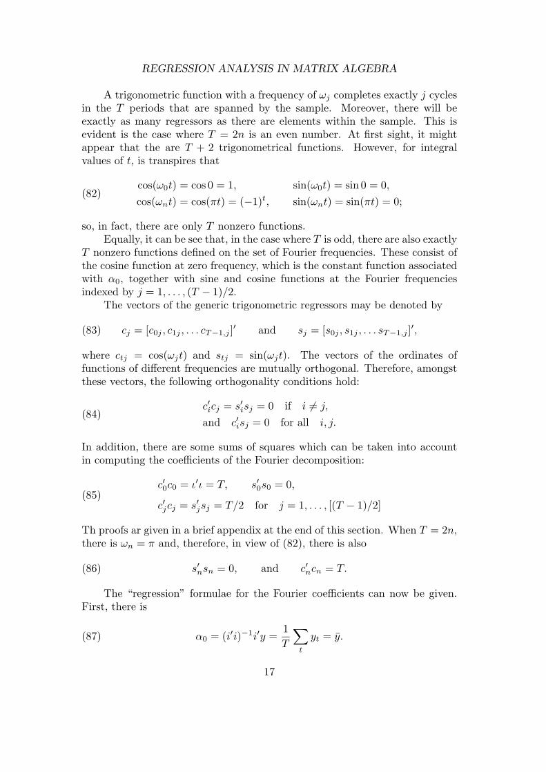
0 25 50 75 100 125Figure 9. The plot of 132 monthly observations on the U.S. money supply,

beginning in January 1960. A quadratic function has been interpolated

through the data.

0

0.005

0.01

0.015

0 π/4 π/2 3π/4 πFigure 10. The periodogram of the residuals of the logarithmic money-

supply data.

if there are no regular harmonic components in the process generating thedata, then we can expect the proportion of the variance attributed to theindividual frequencies to decline as the sample size increases. If there is sucha regular component within the process, then we can expect the proportion ofthe variance attributable to it to converge to a finite value as the sample sizeincreases.

In order provide a graphical representation of the decomposition of thesample variance, we must scale the elements of equation (36) by a factor of T .The graph of the function I(ωj) = (T/2)(α2

j +β2j ) is know as the periodogram.

Figure 9 shows the logarithms of a monthly sequence of 132 observations ofthe US money supply through which a quadratic function has been interpolated.

19


This provides a simple way of characterising the growth of the money supplyover the period in question. The pattern of seasonal fluctuations is remarkablyregular, as can be see from the residuals from the quadratic detrending.

The peridogram of the residual sequence is shown in Figure 10. This has aprominent spike at the frequency value of π/6 radians or 30 degrees per month,which is the fundamental seasonal frequency. Smaller spikes are seen at 60, 90,120, and 150 degrees, which are the harmonics of the fundamental frequency.Their presence reflects the fact that the pattern of the seasonal fluctuations ismore complicated than that of a simple sinusoidal fluctuation at the seasonalfrequency.

The peridodogram also shows a significant spectral mass within the fre-quency range [0π/6]. This mass properly belongs to the trend; and, if thetrend had been adequately estimated, then its effect would not be present inthe residual, which would then show even greater regularity. In lecture 9, wewill show how a more fitting trend function can be estimated.

Appendix: Harmonic Cycles

If a trigonometrical function completes an integral number of cycles in Tperiods, then the sum of its ordinates at the points t = 0, 1, . . . , T − 1 is zero.We state this more formally as follows:

(94) Let ωj = 2πj/T where j ∈ {0, 1, . . . , T/2}, if T is even, andj ∈ {0, 1, . . . , (T − 1)/2}, if T is odd. Then

T−1∑t=0

cos(ωjt) =T−1∑t=0

sin(ωjt) = 0.

Proof. We have

T−1∑t=0

cos(ωjt) =12

T−1∑t=0

{exp(iωjt) + exp(−iωjt)}

=12

T−1∑t=0

exp(i2πjt/T ) +12

T−1∑t=0

exp(−i2πjt/T ).

By using the formula 1 + λ + · · · + λT−1 = (1 − λT )/(1 − λ), we find that

T−1∑t=0

exp(i2πjt/T ) =1 − exp(i2πj)

1 − exp(i2πj/T ).

But Euler’s equation indicates that exp(i2πj) = cos(2πj) + i sin(2πj) = 1, sothe numerator in the expression above is zero, and hence

∑t exp(i2πj/T ) = 0.

20


By similar means, it can be show that∑

t exp(−i2πj/T ) = 0; and, therefore,it follows that

∑t cos(ωjt) = 0.

An analogous proof shows that∑

t sin(ωjt) = 0.

The proposition of (94) is used to establish the orthogonality conditionsaffecting functions with an integral number of cycles.

(95) Let ωj = 2πj/T and ψk = 2πk/T where j, k ∈ 0, 1, . . . , T/2 if Tis even and j, k ∈ 0, 1, . . . , (T − 1)/2 if T is odd. Then

(a)T−1∑t=0

cos(ωjt) cos(ψkt) = 0 ifj �= k,

T−1∑t=0

cos2(ωjt) = T/2,

(b)T−1∑t=0

sin(ωjt) sin(ψkt) = 0 ifj �= k,

T−1∑t=0

sin2(ωjt) = T/2,

(c)T−1∑t=0

cos(ωjt) sin(ψkt) = 0 ifj �= k.

Proof. From the formula cosA cos B = 12{cos(A + B) + cos(A−B)}, we have

T−1∑t=0

cos(ωjt) cos(ψkt) =12

∑{cos([ωj + ψk]t) + cos([ωj − ψk]t)}

=12

T−1∑t=0

{cos(2π[j + k]t/T ) + cos(2π[j − k]t/T )} .

We find, in consequence of (94), that if j �= k, then both terms on the RHSvanish, which gives the first part of (a). If j = k, then cos(2π[j − k]t/T ) =cos 0 = 1 and so, whilst the first term vanishes, the second terms yields thevalue of T under summation. This gives the second part of (a).

The proofs of (b) and (c) follow along similar lines once the relevanttrigonometrical identities have been invoked.

21

Regression Analysis - University of Leicester€¦ · LECTURE 2 Regression Analysis The Multiple...

Documents

Transcript of Regression Analysis - University of Leicester€¦ · LECTURE 2 Regression Analysis The Multiple...