Regression analysis Regression Models

Chapter 4

Regression Models

© 2008 Prentice-Hall, Inc.Quantitative Analysis for Management, Tenth Edition,by Render, Stair, and Hanna

Introduction

�� Regression analysisRegression analysis is a very valuable tool for a manager

� There are generally two purposes for regression analysis

4 – 2

regression analysis1. To understand the relationship between

variables� E.g. the relationship between the sales volume

and the advertising spending amount, the relationship between the price of a house and the square footage, etc.

2. To predict the value of one variable based on the value of another variable

Introduction

� Simple linear regression models have only two variables

Three types of regression models will be studied

4 – 3

only two variables� We will first develop this model

� Multiple regression models have more than two variables

� Nonlinear regression models are used when the relationships between the variables are not linear

Introduction

� The variable to be predicted is called the dependent variabledependent variable� Sometimes called the response variableresponse variable

� The value of this variable depends on the value of the independent variableindependent variable

4 – 4

the value of the independent variableindependent variable� Sometimes called the explanatoryexplanatory or

predictor variablepredictor variable

Independent variable1

Dependent variable

Independent variable2= + + ...

Prediction Relationship

Scatter Diagram

� One way to investigate the relationship between variables is by plotting the data on a graph

� Such a graph is often called a scatter scatter diagramdiagram or a scatter plotscatter plot

4 – 5

diagramdiagram or a scatter plotscatter plot� The independent variable is normally

plotted on the X axis� The dependent variable is normally

plotted on the Y axis

� Triple A Construction renovates old homes� They have found that the dollar volume of

renovation work each year is dependent on the area payroll

� Triple A’s revenues and the total wage earnings for the past six years are listed below

Triple A Construction Example

4 – 6

for the past six years are listed below

TRIPLE A’S SALES($100,000’s)

LOCAL PAYROLL($100,000,000’s)

6 38 49 65 44.5 29.5 5Table 4.1

dependentdependentvariablevariable

independentindependentvariablevariable


12 –

10 –

8 –

Sal

es (

$100

,000

)

4 – 7

Figure 4.1: Scatter Diagram for Triple A Constructi on Company Data in Table 4.1

6 –

4 –

2 –

0 –

Sal

es (

$100

,000

)

Payroll ($100 million)

| | | | | | | |0 1 2 3 4 5 6 7 8

� The graph indicates higher payroll seem to result in higher sales

� A line has been drawn to show the relationship between the payroll and the sales

� There is not a perfect relationship because not


4 – 8

� There is not a perfect relationship because not all points lie in a straight line

� Errors are involved if this line is used to predict sales based on payroll

� Many lines could be drawn through these points, but which one best represents the true relationship ?

Simple Linear Regression

� Regression models are used to find the relationship between variables – i.e. to predict the value of one variable based on the other

4 – 9

� However there is some random error that cannot be predicted

� Regression models can also be used to test if a relationship exists between variables


� The underlying simple linear regression model is:

εεεεββββββββ ++++++++==== XY 10

4 – 10

whereY = dependent variable (response)X = independent variable (predictor or

explanatory)ββββ0 = intercept (value of Y when X = 0)ββββ1 = slope of the regression line εεεε = random error


� The random error cannot be predicted. So an approximation of the model is used

XbbY 10 ++++====ˆ

4 – 11

XbbY 10 ++++====

where

Y = predicted value of YX = independent variable (predictor or

explanatory)b0 = estimate of ββββ0

b1 = estimate of ββββ1

^

Triple A Construction

� Triple A Construction is trying to predict sales based on area payroll

Y = SalesX = Area payroll

4 – 12

X = Area payroll

� The line chosen in Figure 4.1 is the one that best fits the sample data by minimizing the sum of all errors

Error = (Actual value) – (Predicted value)

YYe ˆ−−−−====


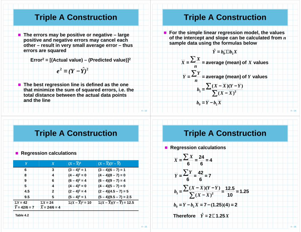
� The errors may be positive or negative – large positive and negative errors may cancel each other – result in very small average error – thus errors are squared

Error 2 = [(Actual value) – (Predicted value)] 2

4 – 13

Error 2 = [(Actual value) – (Predicted value)] 2

22 )Y(Ye ˆ−−−−====

� The best regression line is defined as the one that minimize the sum of squared errors, i.e. the total distance between the actual data points and the line


� For the simple linear regression model, the values of the intercept and slope can be calculated from nsample data using the formulas below

XbbY 10 ++++====ˆ

X∑∑∑∑

4 – 14

values of (mean) average Xn

XX ======== ∑∑∑∑

values of (mean) average Yn

YY ======== ∑∑∑∑

∑∑∑∑∑∑∑∑

−−−−−−−−−−−−

==== 21 )(

))((

XX

YYXXb

XbYb 10 −−−−====


Y X (X – X)2 (X – X)(Y – Y)

6 3 (3 – 4)2 = 1 (3 – 4)(6 – 7) = 18 4 (4 – 4)2 = 0 (4 – 4)(8 – 7) = 0

� Regression calculations

4 – 15

8 4 (4 – 4)2 = 0 (4 – 4)(8 – 7) = 09 6 (6 – 4)2 = 4 (6 – 4)(9 – 7) = 45 4 (4 – 4)2 = 0 (4 – 4)(5 – 7) = 04.5 2 (2 – 4)2 = 4 (2 – 4)(4.5 – 7) = 5

9.5 5 (5 – 4)2 = 1 (5 – 4)(9.5 – 7) = 2.5

ΣY = 42Y = 42/6 = 7

ΣX = 24X = 24/6 = 4

Σ(X – X)2 = 10 Σ(X – X)(Y – Y) = 12.5

Table 4.2


46

246

============ ∑∑∑∑X

X

742 ============ ∑∑∑∑

YY


4 – 16

7642

6============ ∑∑∑∑

YY

25110

51221 .

.)(

))((========

−−−−−−−−−−−−

====∑∑∑∑

∑∑∑∑XX

YYXXb

24251710 ====−−−−====−−−−==== ))(.(XbYb

XY 2512 .ˆ ++++====Therefore


46

246

============ ∑∑∑∑X

X

742 ============ ∑∑∑∑

YY


sales = 2 + 1.25(payroll)

If the payroll next year is $600 million

4 – 17

7642

6============ ∑∑∑∑

YY

25110

51221 .

.)(

))((========

−−−−−−−−−−−−

====∑∑∑∑

∑∑∑∑XX

YYXXb

24251710 ====−−−−====−−−−==== ))(.(XbYb

XY 2512 .ˆ ++++====Therefore

year is $600 million

000950 $ or 5962512 ,.)(.ˆ ====++++====Y

Measuring the Fit of the Regression Model

� Regression models can be developed for any variables X and Y

� How do we know the model is good enough (with small errors) in predicting Ybased on X ?

4 – 18

based on X ?� The following measures are useful in

describing the accuracy of the model� Three measures of variability

� SST – Total variability about the mean� SSE – Variability about the regression line� SSR – Total variability that is explained by the

model


� Sum of the squares total2)(∑∑∑∑ −−−−==== YYSST

� Sum of the squared error

∑∑∑∑ ∑∑∑∑ −−−−======== 22 )ˆ( YYeSSE

4 – 19

∑∑∑∑ ∑∑∑∑ −−−−======== 22 )ˆ( YYeSSE

� Sum of squares due to regression

∑∑∑∑ −−−−==== 2)ˆ( YYSSR

� An important relationshipSSESSRSST ++++====


Y X (Y – Y)2 Y (Y – Y)2 (Y – Y)2

6 3 (6 – 7)2 = 1 2 + 1.25(3) = 5.75 0.0625 1.563

8 4 (8 – 7)2 = 1 2 + 1.25(4) = 7.00 1 0

9 6 (9 – 7)2 = 4 2 + 1.25(6) = 9.50 0.25 6.25

^ ^^

4 – 20

9 6 (9 – 7)2 = 4 2 + 1.25(6) = 9.50 0.25 6.25

5 4 (5 – 7)2 = 4 2 + 1.25(4) = 7.00 4 0

4.5 2 (4.5 – 7)2 = 6.25 2 + 1.25(2) = 4.50 0 6.25

9.5 5 (9.5 – 7)2 = 6.25 2 + 1.25(5) = 8.25 1.5625 1.563

∑(Y – Y)2 = 22.5 ∑(Y – Y)2 = 6.875 ∑(Y – Y)2 = 15.625

Y = 7 SST = 22.5 SSE = 6.875 SSR = 15.625

^^

Table 4.3


� SST = 22.5 is the variability of the prediction using mean value of Y

� SSE = 6.875 is the variability of the prediction using regression line

� Prediction using regression line has reduced the

4 – 21

� Prediction using regression line has reduced the variability by 22.5 −−−− 6.875 = 15.625

� SSR = 15.625 indicates how much of the total variability in Y is explained by the regression model

� Note: SST = SSR + SSE� SSR – explained variability� SSE – unexplained variability


12 –

10 –

8 –

Sal

es (

$100

,000

)

Y = 2 + 1.25X^

Y

Y – Y^(SSE)

Y – Y^(SSR)Y – Y (SST)

4 – 22

Figure 4.2

6 –

4 –

2 –

0 –

Sal

es (

$100

,000

)

Payroll ($100 million)

| | | | | | | |0 1 2 3 4 5 6 7 8

Coefficient of Determination

� The proportion of the variability in Y explained by regression equation is called the coefficient of coefficient of determinationdetermination

� The coefficient of determination is r2

SSESSRr −−−−======== 12

4 – 23

SSTSSE

SSTSSR

r −−−−======== 12

� For Triple A Construction

69440522

625152 ..

. ========r

� About 69% of the variability in Y is explained by the equation based on payroll ( X)

� If SSE �� 0, then r 2 �� 100%

Correlation Coefficient

� The correlation coefficientcorrelation coefficient is an expression of the strength of the linear relationship between the variables

� It will always be between +1 and –1

2rr ±±±±====

4 – 24

� It will always be between +1 and –1� Negative slope �� r < 0; positive slope �� r > 0� The correlation coefficient is r� For Triple A Construction

8333069440 .. ========r

Correlation Coefficient

**

*

*

Y

* ***

*

Y

****

*

**

4 – 25

(a) Perfect PositiveCorrelation: r = +1

X

*

* *

*(c) No Correlation:

r = 0X

Y

* **

** *

* ***

(d) Perfect Negative Correlation: r = –1

X

Y

**

**

*(b) Positive

Correlation: 0 < r < 1

X

Figure 4.3

Using Computer Software for Regression

4 – 26

Program 4.1A


4 – 27

Program 4.1B


4 – 28

Program 4.1C


Correlation coefficient ( r) is Multiple R in Excel

4 – 29

Program 4.1D 1.25X2Y ++++====ˆ

Assumptions of the Regression Model

1. Errors are independent2. Errors are normally distributed

� If we make certain assumptions about the errors in a regression model, we can perform statistical tests to determine if the model is useful

4 – 30

2. Errors are normally distributed3. Errors have a mean of zero4. Errors have a constant variance

� A plot of the residuals (errors) will often highlig ht any glaring violations of the assumption

Residual Plots

� A random plot of residuals� Healthy pattern – no violations

4 – 31

Figure 4.4A

Err

or

X

Error = 0

Residual Plots

� Nonconstant error variance – violation � Errors increase as X increases, violating the

constant variance assumption

4 – 32

Figure 4.4B

Err

or

X

Error = 0

Residual Plots

� Nonlinear relationship – violation � Errors consistently increasing and then consistentl y

decreasing indicate that the model is not linear (perhaps quadratic)

4 – 33

Figure 4.4C

Err

or

X

Error = 0

Estimating the Variance

� Errors are assumed to have a constant variance ( σσσσ 2), but we usually don’t know this

� It can be estimated using the mean mean squared errorsquared error (MSEMSE), s2

4 – 34

squared errorsquared error (MSEMSE), s2

12

−−−−−−−−========

knSSE

MSEs

wheren = number of observations in the samplek = number of independent variables

Estimating the Variance

� For Triple A Construction

718814

87506116

875061

2 ... ========

−−−−−−−−====

−−−−−−−−========

knSSE

MSEs

4 – 35

� We can estimate the standard deviation, s� This is also called the standard error of the standard error of the

estimateestimate or the standard deviation of the standard deviation of the regressionregression

31171881 .. ============ MSEs

� A small s2 or s means the actual data deviate within a small range from the predicted result

Testing the Model for Significance

� Both r2 and the MSE (s2) provide a measure of accuracy in a regression model

� However when the sample size is too small, you can get good values for MSE and r2

even if there is no relationship between the

4 – 36

even if there is no relationship between the variables

� Testing the model for significance helps determine if r2 and MSE are meaningful and if a linear relationship exists between the variables

� We do this by performing a statistical hypothesis test


� We start with the general linear model

εεεεββββββββ ++++++++==== XY 10

� If ββββ1 = 0, the null hypothesis is that there is nono relationship between X and Y

4 – 37

nono relationship between X and Y� The alternate hypothesis is that there isis a

linear relationship ( ββββ1 ≠ 0)� If the null hypothesis can be rejected, we

have proven there is a linear relationship� We use the F statistic for this test

� A continuous probability distribution (Fig. 2.15)� The area underneath the curve represents

probability of the F statistic value falling within a particular interval.

� The F statistic is the ratio of two sample variances

The F Distribution

4 – 38

� The F statistic is the ratio of two sample variances� F distributions have two sets of degrees of

freedom� Degrees of freedom are based on sample size and

used to calculate the numerator and denominator

df1 = degrees of freedom for the numeratordf2 = degrees of freedom for the denominator

The F Distribution

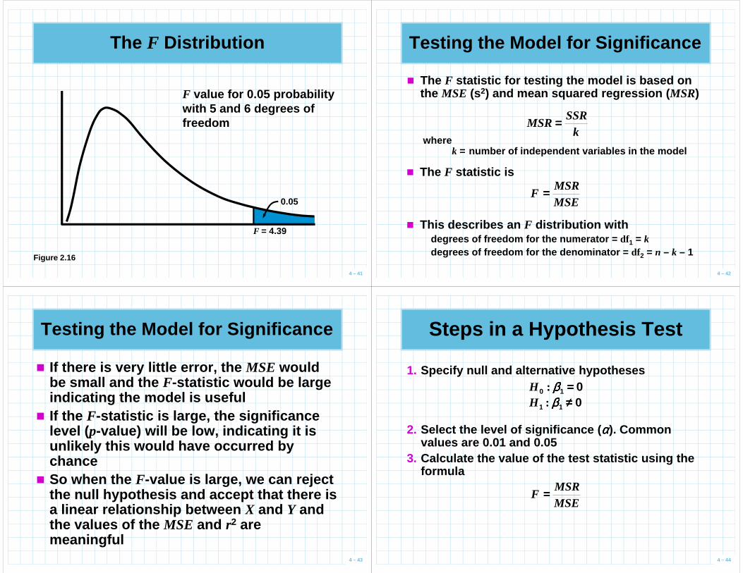
df1 = 5df2 = 6αααα = 0.05 (probability)

Consider the example:

From Appendix D, we get

4 – 39

From Appendix D, we get

Fαααα, df1, df2 = F0.05, 5, 6 = 4.39

This means

P(F > 4.39) = 0.05

There is only a 5% probability that F will exceed 4.39 (see Fig. 2.16)

The F Distribution

4 – 40

Fα

Figure 2.15

The F Distribution

F value for 0.05 probability with 5 and 6 degrees of freedom

4 – 41

Figure 2.16

F = 4.39

0.05


� The F statistic for testing the model is based on the MSE (s2) and mean squared regression ( MSR)

kSSR

MSR ====where

4 – 42

wherek = number of independent variables in the model

� The F statistic is

MSEMSR

F ====

� This describes an F distribution withdegrees of freedom for the numerator = df1 = kdegrees of freedom for the denominator = df2 = n – k – 1


� If there is very little error, the MSE would be small and the F-statistic would be large indicating the model is useful

� If the F-statistic is large, the significance level ( p-value) will be low, indicating it is

4 – 43

level ( p-value) will be low, indicating it is unlikely this would have occurred by chance

� So when the F-value is large, we can reject the null hypothesis and accept that there is a linear relationship between X and Y and the values of the MSE and r2 are meaningful

Steps in a Hypothesis Test

1. Specify null and alternative hypotheses010 ====ββββ:H011 ≠≠≠≠ββββ:H

2. Select the level of significance ( αααα). Common

4 – 44

2. Select the level of significance ( αααα). Common values are 0.01 and 0.05

3. Calculate the value of the test statistic using the formula

MSEMSR

F ====

Steps in a Hypothesis Test

4. Make a decision using one of the following methodsa) Reject the null hypothesis if the test statistic is

greater than the FF--valuevalue from the table in Appendix D. Otherwise, do not reject the null hypothesis:

4 – 45

21 ifReject dfdfcalculated FF ,,αααα>>>>

kdf ====1

12 −−−−−−−−==== kndf

b) Reject the null hypothesis if the observed signific ance level, or pp--value,value, is less than the level of significance (αααα). Otherwise, do not reject the null hypothesis:

)( statistictest calculatedvalue- >>>>==== FPpαααα<<<<value- ifReject p

Triple A ConstructionStep 1.Step 1.

H0: ββββ1 = 0 (no linear relationship between X and Y)

H1: ββββ1 ≠ 0 (linear relationship exists between X and Y)

Step 2.Step 2.

4 – 46

Step 2.Step 2.Select αααα = 0.05

6250151625015

.. ============

kSSR

MSR

09971881625015

... ============

MSEMSR

F

Step 3.Step 3.Calculate the value of the test statistic

Triple A ConstructionStep 4.Step 4.

Reject the null hypothesis if the test statistic is greater than the F-value in Appendix D

df1 = k = 1df2 = n – k – 1 = 6 – 1 – 1 = 4

4 – 47

df2 = n – k – 1 = 6 – 1 – 1 = 4

The value of F associated with a 5% level of significance and with degrees of freedom 1 and 4 is found in Appendix D

F0.05,1,4 = 7.71Fcalculated = 9.09Reject H0 because 9.09 > 7.71


� We can conclude there is a statistically significant relationship between X and Y

� The r2 value of 0.69 means about 69% of the variability in

4 – 48

F = 7.71

0.05

9.09Figure 4.5

about 69% of the variability in sales ( Y) is explained by local payroll ( X)


� The F-test determines whether or not there is a relationship between the variables

� r2 (coefficient of determination) is the best measure of the strength of the prediction

4 – 49

measure of the strength of the prediction relationship between the X and Y variables� Values closer to 1 indicate a strong prediction

relationship� Good regression models have a low

significance level for the F-test and high r2

value.

Analysis of Variance (ANOVA) Table

� When software is used to develop a regression model, an ANOVA table is typically created that shows the observed significance level ( p-value) for the calculated F value

� This can be compared to the level of significance (αααα) to make a decision

4 – 50

(αααα) to make a decision

DF SS MS F SIGNIFICANCE

Regression k SSR MSR = SSR/k MSR/MSE P(F > MSR/MSE)

Residual n - k - 1 SSE MSE = SSE/(n - k - 1)

Total n - 1 SST

Table 4.4

ANOVA for Triple A Construction

4 – 51

� Because this probability is less than 0.05, we reject the null hypothesis of no linear relationshi p and conclude there is a linear relationship between X and Y

Program 4.1D (partial)

P(F > 9.0909) = 0.0394

Multiple Regression Analysis

�� Multiple regression modelsMultiple regression models are extensions to the simple linear model and allow the creation of models with several independent variables

4 – 52

Y = ββββ0 + ββββ1X1 + ββββ2X2 + … + ββββkXk + εεεεwhere

Y = dependent variable (response variable)Xi = ith independent variable (predictor or explanatory

variable)ββββ0 = intercept (value of Y when all Xi = 0)ββββI = coefficient of the ith independent variablek = number of independent variablesεεεε = random error

Multiple Regression Analysis

� To estimate these values, samples are taken and the following equation is developed

kk XbXbXbbY ++++++++++++++++==== ...ˆ22110

4 – 53

where= predicted value of Y

b0 = sample intercept (and is an estimate of ββββ0)bi = sample coefficient of the ith variable (and is

an estimate of ββββi)

Y

Jenny Wilson Realty

� Jenny Wilson wants to develop a model to determine the suggested listing price for houses based on the size and age of the house

22110ˆ XbXbbY ++++++++====

where

4 – 54

where= predicted value of dependent variable (selling pri ce)

b0 = Y interceptX1 and X2 = value of the two independent variables (square

footage and age) respectivelyb1 and b2 = slopes for X1 and X2 respectively

Y

� She selects a few samples of the houses sold recently and records the data shown in Table 4.5

� She also saves information on house condition to be used later

Jenny Wilson RealtySELLING PRICE ($)

SQUARE FOOTAGE AGE CONDITION

95,000 1,926 30 Good

119,000 2,069 40 Excellent

124,800 1,720 30 Excellent

135,000 1,396 15 Good

142,000 1,706 32 Mint

4 – 55

142,000 1,706 32 Mint

145,000 1,847 38 Mint

159,000 1,950 27 Mint

165,000 2,323 30 Excellent

182,000 2,285 26 Mint

183,000 3,752 35 Good

200,000 2,300 18 Good

211,000 2,525 17 Good

215,000 3,800 40 Excellent

219,000 1,740 12 MintTable 4.5

Jenny Wilson Realty

4 – 56

Program 4.221 289944146631 XXY −−−−++++====ˆ

0021788.0

Evaluating Multiple Regression Models

� Evaluation is similar to simple linear regression models� The p-value for the F-test and r2 are

interpreted the same

4 – 57

� The hypothesis is different because there is more than one independent variable� The F-test is investigating whether all

the coefficients are equal to 0� If the F-test is significant, it does not

mean all independent variables are significant

Evaluating Multiple Regression Models

� To determine which independent variables are significant, tests are performed for each variable

010 ====ββββ:H

4 – 58

010 ====ββββ:H011 ≠≠≠≠ββββ:H

� The test statistic is calculated and if the p-value is lower than the level of significance ( αααα), the null hypothesis is rejected

Jenny Wilson Realty

� The model is statistically significant� The p-value for the F-test is 0.002� r2 = 0.6719 so the model explains about 67% of

the variation in selling price ( Y)� But the F-test is for the entire model and we can’t

4 – 59

� But the F-test is for the entire model and we can’t tell if one or both of the independent variables ar e significant

� By calculating the p-value of each variable, we can assess the significance of the individual variables

� Since the p-value for X1 (square footage) and X2(age) are both less than the significance level of 0.05, both null hypotheses can be rejected

Binary or Dummy Variables

�� BinaryBinary (or dummydummy or indicatorindicator) variables are special variables created for qualitative data

� A binary variable is assigned a value of 1 if a particular qualitative condition is met and

4 – 60

a particular qualitative condition is met and a value of 0 otherwise

� Adding binary variables may increase the accuracy of the regression model

� The number of binary variables must be one less than the number of categories of the qualitative variable

Jenny Wilson Realty

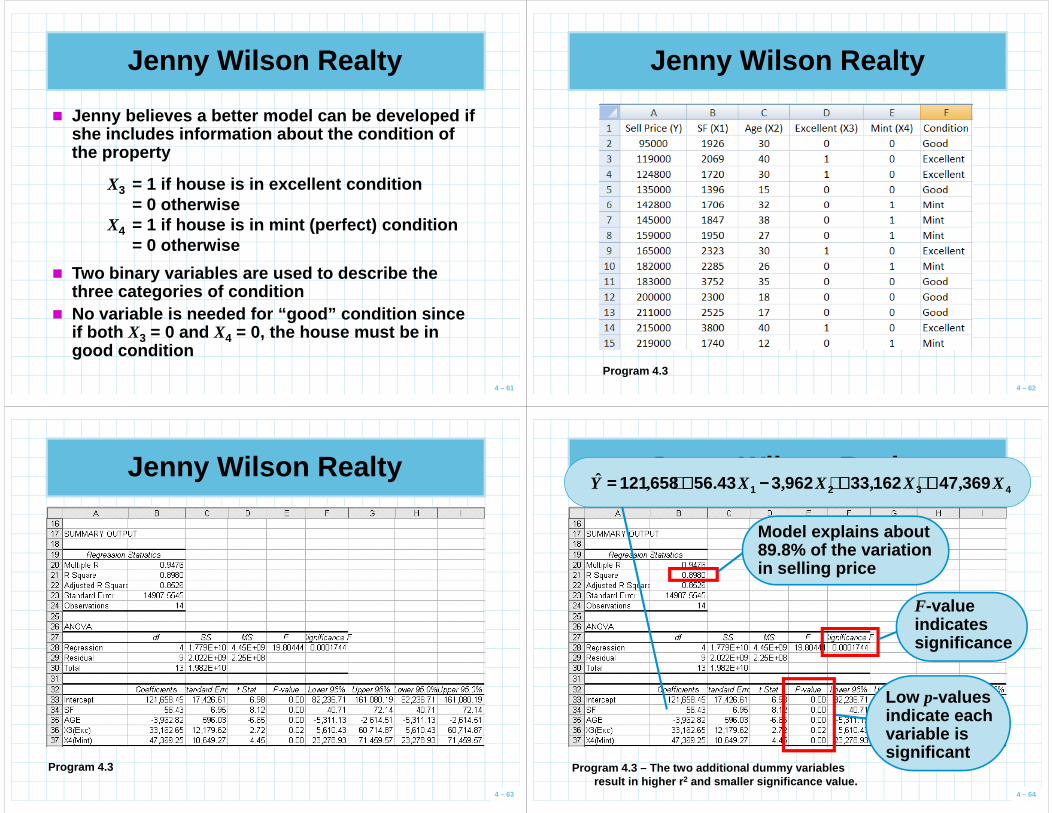
� Jenny believes a better model can be developed if she includes information about the condition of the property

X3 = 1 if house is in excellent condition= 0 otherwise

4 – 61

= 0 otherwiseX4 = 1 if house is in mint (perfect) condition

= 0 otherwise

� Two binary variables are used to describe the three categories of condition

� No variable is needed for “good” condition since if both X3 = 0 and X4 = 0, the house must be in good condition

Jenny Wilson Realty

4 – 62

Program 4.3

Jenny Wilson Realty

4 – 63

Program 4.3

Jenny Wilson Realty

Model explains about 89.8% of the variation in selling price

F-value

4321 369471623396234356658121 XXXXY ,,,.,ˆ ++++++++−−−−++++====

4 – 64

Program 4.3 – The two additional dummy variablesresult in higher r2 and smaller significance value.

F-value indicates significance

Low p-values indicate each variable is significant

Model Building

� The best model is a statistically significant model with a high r2 and few variables

� As more variables are added to the model, the r2-value usually increasesHowever more variables does not

4 – 65

� However more variables does not necessarily mean better model

� For this reason, the adjusted adjusted rr22 value is often used to determine if additional independent variable is beneficial

� The adjusted r2 takes into account the number of independent variables in the model

Model Building

SSTSSE

SSTSSR −−−−======== 12r

� The formula for r2

� The formula for adjusted r2

4 – 66

� The formula for adjusted r2

)/(SST)/(SSE

11

1 Adjusted 2

−−−−−−−−−−−−−−−−====

nkn

r

� As the number of independent variables ( k) increases, n-k-1 decreases. This causes SSE/(n-k-1)to increase and the adjusted r2 to decrease unless the extra variable causes a significant decrease in the SSE(and error) to offset the change in k

Model Building

� Note when new variables are added to the model, the value of r2 will never decrease; however the adjusted r2 may decrease

� In general, if a new variable increases the adjusted r2, it should probably be included in

4 – 67

In general, if a new variable increases the adjusted r2, it should probably be included in the model

� A variable should not be added to the model if it causes the adjusted r2 to decrease

� Compare the adjusted r2 before and after adding the two binary variables in Jenny Wilson Realty example (0.6122 vs 0.8526)

Model Building

� In some cases, variables contain duplicate information� E.g. size of the lot, # of bedrooms and # of

bathrooms might be correlated with the square footage of the house

When two independent variables are correlated,

4 – 68

� When two independent variables are correlated, they are said to be collinearcollinear

� When more than two independent variables are correlated, multicollinearitymulticollinearity exists

� The model is still good for prediction purpose when multicollinearity is present

� But hypothesis tests (p-values) for the individual variables and the interpretation of their coefficie nts are not valid

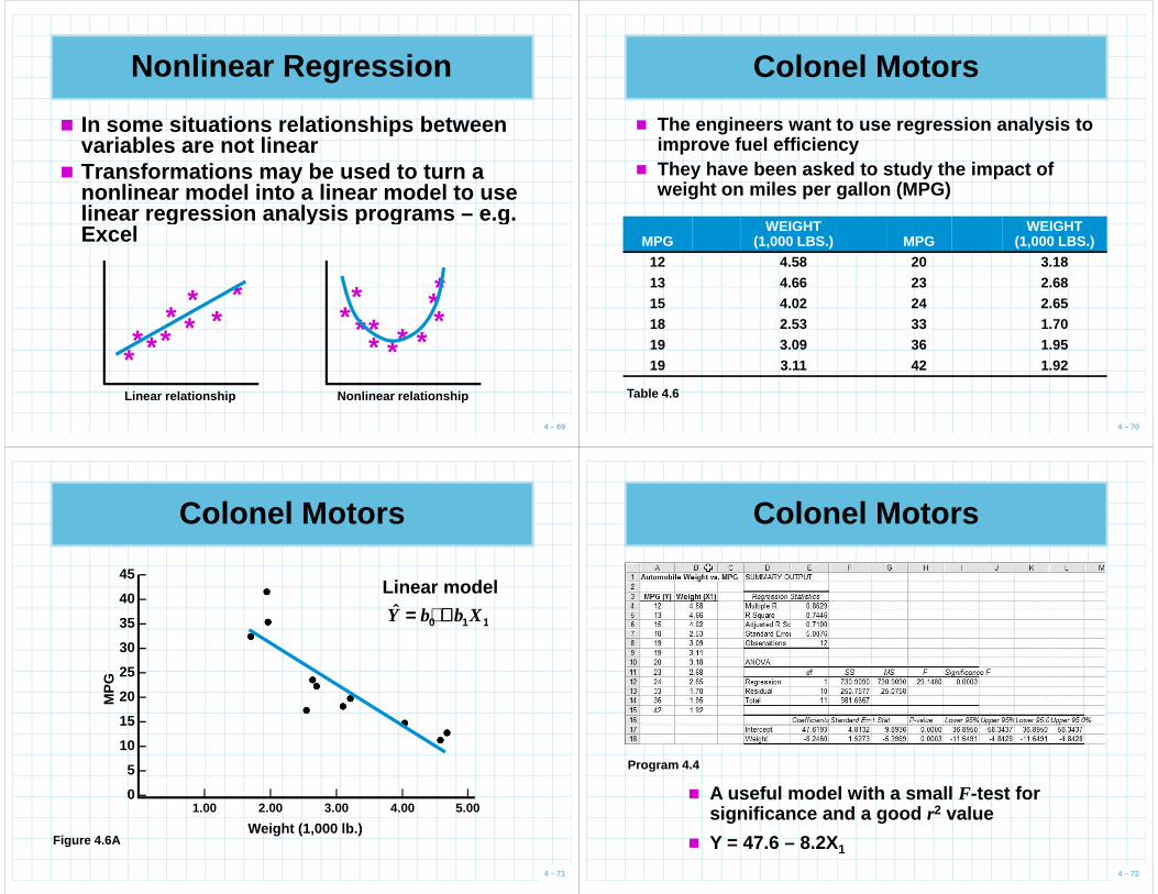
Nonlinear Regression

� In some situations relationships between variables are not linear

� Transformations may be used to turn a nonlinear model into a linear model to use linear regression analysis programs – e.g. Excel

4 – 69

linear regression analysis programs – e.g. Excel

** **

** ** *

Linear relationship Nonlinear relationship

* *** **

****

*

Colonel Motors

� The engineers want to use regression analysis to improve fuel efficiency

� They have been asked to study the impact of weight on miles per gallon (MPG)

WEIGHT WEIGHT

4 – 70

MPGWEIGHT

(1,000 LBS.) MPGWEIGHT

(1,000 LBS.)12 4.58 20 3.1813 4.66 23 2.6815 4.02 24 2.6518 2.53 33 1.7019 3.09 36 1.9519 3.11 42 1.92

Table 4.6

Colonel Motors

45 –

40 –

35 –

30 –

25 –

��

��

��

Linear model

110 XbbY ++++====ˆ

4 – 71

Figure 4.6A

25 –

20 –

15 –

10 –

5 –

0 – | | | | |

1.00 2.00 3.00 4.00 5.00

MP

G

Weight (1,000 lb.)

��

��

��

��

Colonel Motors

4 – 72

Program 4.4

� A useful model with a small F-test for significance and a good r2 value

� Y = 47.6 – 8.2X1

Colonel Motors

45 –

40 –

35 –

30 –

��

��

��

A nonlinear model seams better2

210 weightweight )()(MPG bbb ++++++++====

4 – 73

Figure 4.6B

25 –

20 –

15 –

10 –

5 –

0 – | | | | |

1.00 2.00 3.00 4.00 5.00

MP

G

Weight (1,000 lb.)

��

��

��

��

Colonel Motors

� The nonlinear model is a quadratic model� The easiest way to work with this model is to

develop a new variable

22 weight )(====X

4 – 74

2

� This gives us a model that can be solved with linear regression software

22110 XbXbbY ++++++++====ˆ

Colonel Motors

21 43230879 XXY ...ˆ ++++−−−−====

4 – 75

Program 4.5

� A better model with a smaller F-test for significance and a larger adjusted r2 value

� Interpretation of coefficients and P-values are not valid

Cautions and Pitfalls

� If the assumptions about the errors are not met, the statistical test may not be valid

� Correlation does not necessarily mean causation (e.g. price of automobiles and your annual salary)

4 – 76

your annual salary)� Multicollinearity makes interpreting

coefficients problematic, but the model may still be good

� Using a regression model beyond the range of X is questionable, the relationship may not hold outside the sample data (e.g. advertising amount and sales volume)

Cautions and Pitfalls

� t-tests for the intercept ( b0) may be ignored as this point ( X=0) is often outside the range of the model

� A linear relationship may not be the best relationship, even if the F-test returns an

4 – 77

relationship, even if the F-test returns an acceptable value

� A nonlinear relationship can exist even if a linear relationship does not

� Just because a relationship is statistically significant doesn't mean it has any practical value – r2 must also be significant

Homework Assignment

http://www.sci.brooklyn.cuny.edu/~dzhu/busn3430/

4 – 78

Regression analysis Regression Models

Documents

Transcript of Regression analysis Regression Models