Lecture 3: Loss Functions and...
85
Fei-Fei Li & Justin Johnson & Serena Yeung Lecture 3 - April 11, 2017 1 Lecture 3: Loss Functions and Optimization
Transcript of Lecture 3: Loss Functions and...

Fei-Fei Li & Justin Johnson & Serena Yeung Lecture 3 - April 11, 20171
Lecture 3:Loss Functions
and Optimization

Fei-Fei Li & Justin Johnson & Serena Yeung Lecture 3 - April 11, 2017
Administrative
Assignment 1 is released: http://cs231n.github.io/assignments2017/assignment1/
Due Thursday April 20, 11:59pm on Canvas
(Extending due date since it was released late)
2

Fei-Fei Li & Justin Johnson & Serena Yeung Lecture 3 - April 11, 2017
Administrative
Check out Project Ideas on Piazza
Schedule for Office hours is on the course website
TA specialties are posted on Piazza
3

Fei-Fei Li & Justin Johnson & Serena Yeung Lecture 3 - April 11, 2017
Administrative
4
Details about redeeming Google Cloud Credits should go out today;will be posted on Piazza
$100 per student to use for homeworks and projects

Fei-Fei Li & Justin Johnson & Serena Yeung Lecture 3 - April 11, 2017
Recall from last time: Challenges of recognition
5
This image is CC0 1.0 public domain This image by Umberto Salvagnin is licensed under CC-BY 2.0
This image by jonsson is licensed under CC-BY 2.0
Illumination Deformation Occlusion
This image is CC0 1.0 public domain
Clutter
This image is CC0 1.0 public domain
Intraclass Variation
Viewpoint
Fei-Fei Li & Justin Johnson & Serena Yeung Lecture 3 - April 11, 2017
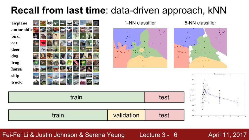
Recall from last time: data-driven approach, kNN
6
1-NN classifier 5-NN classifier
train test
train testvalidation

Fei-Fei Li & Justin Johnson & Serena Yeung Lecture 3 - April 11, 2017
Recall from last time: Linear Classifier
7
f(x,W) = Wx + b

Fei-Fei Li & Justin Johnson & Serena Yeung Lecture 3 - April 11, 2017
Recall from last time: Linear Classifier
8
1. Define a loss function that quantifies our unhappiness with the scores across the training data.
2. Come up with a way of efficiently finding the parameters that minimize the loss function. (optimization)
TODO:
Cat image by Nikita is licensed under CC-BY 2.0; Car image is CC0 1.0 public domain; Frog image is in the public domain

Fei-Fei Li & Justin Johnson & Serena Yeung Lecture 3 - April 11, 20179
cat
frog
car
3.25.1-1.7
4.91.3
2.0 -3.12.52.2
Suppose: 3 training examples, 3 classes.With some W the scores are:

Fei-Fei Li & Justin Johnson & Serena Yeung Lecture 3 - April 11, 201710
cat
frog
car
3.25.1-1.7
4.91.3
2.0 -3.12.52.2
Suppose: 3 training examples, 3 classes.With some W the scores are:
A loss function tells how good our current classifier is
Given a dataset of examples
Where is image and is (integer) label
Loss over the dataset is a sum of loss over examples:

Fei-Fei Li & Justin Johnson & Serena Yeung Lecture 3 - April 11, 201711
cat
frog
car
3.25.1-1.7
4.91.3
2.0 -3.12.52.2
Suppose: 3 training examples, 3 classes.With some W the scores are:
Multiclass SVM loss:
Given an examplewhere is the image andwhere is the (integer) label,
and using the shorthand for the scores vector:
the SVM loss has the form:

Fei-Fei Li & Justin Johnson & Serena Yeung Lecture 3 - April 11, 201712
cat
frog
car
3.25.1-1.7
4.91.3
2.0 -3.12.52.2
Suppose: 3 training examples, 3 classes.With some W the scores are:
Multiclass SVM loss:
Given an examplewhere is the image andwhere is the (integer) label,
and using the shorthand for the scores vector:
the SVM loss has the form:
“Hinge loss”

Fei-Fei Li & Justin Johnson & Serena Yeung Lecture 3 - April 11, 201713
cat
frog
car
3.25.1-1.7
4.91.3
2.0 -3.12.52.2
Suppose: 3 training examples, 3 classes.With some W the scores are:
Multiclass SVM loss:
Given an examplewhere is the image andwhere is the (integer) label,
and using the shorthand for the scores vector:
the SVM loss has the form:

Fei-Fei Li & Justin Johnson & Serena Yeung Lecture 3 - April 11, 201714
cat
frog
car
3.25.1-1.7
4.91.3
2.0 -3.12.52.2
Suppose: 3 training examples, 3 classes.With some W the scores are:
Multiclass SVM loss:
Given an examplewhere is the image andwhere is the (integer) label,
and using the shorthand for the scores vector:
the SVM loss has the form:
= max(0, 5.1 - 3.2 + 1) +max(0, -1.7 - 3.2 + 1)= max(0, 2.9) + max(0, -3.9)= 2.9 + 0= 2.9Losses: 2.9

Fei-Fei Li & Justin Johnson & Serena Yeung Lecture 3 - April 11, 201715
cat
frog
car
3.25.1-1.7
4.91.3
2.0 -3.12.52.2
Suppose: 3 training examples, 3 classes.With some W the scores are:
Multiclass SVM loss:
Given an examplewhere is the image andwhere is the (integer) label,
and using the shorthand for the scores vector:
the SVM loss has the form:
Losses:
= max(0, 1.3 - 4.9 + 1) +max(0, 2.0 - 4.9 + 1)= max(0, -2.6) + max(0, -1.9)= 0 + 0= 002.9

Fei-Fei Li & Justin Johnson & Serena Yeung Lecture 3 - April 11, 201716
cat
frog
car
3.25.1-1.7
4.91.3
2.0 -3.12.52.2
Suppose: 3 training examples, 3 classes.With some W the scores are:
Multiclass SVM loss:
Given an examplewhere is the image andwhere is the (integer) label,
and using the shorthand for the scores vector:
the SVM loss has the form:
Losses:
= max(0, 2.2 - (-3.1) + 1) +max(0, 2.5 - (-3.1) + 1)= max(0, 6.3) + max(0, 6.6)= 6.3 + 6.6= 12.912.92.9 0

Fei-Fei Li & Justin Johnson & Serena Yeung Lecture 3 - April 11, 201717
cat
frog
car
3.25.1-1.7
4.91.3
2.0 -3.12.52.2
Suppose: 3 training examples, 3 classes.With some W the scores are:
Multiclass SVM loss:
Given an examplewhere is the image andwhere is the (integer) label,
and using the shorthand for the scores vector:
the SVM loss has the form:
Loss over full dataset is average:
Losses: 12.92.9 0 L = (2.9 + 0 + 12.9)/3 = 5.27

Fei-Fei Li & Justin Johnson & Serena Yeung Lecture 3 - April 11, 201718
cat
frog
car
3.25.1-1.7
4.91.3
2.0 -3.12.52.2
Suppose: 3 training examples, 3 classes.With some W the scores are:
Multiclass SVM loss:
Given an examplewhere is the image andwhere is the (integer) label,
and using the shorthand for the scores vector:
the SVM loss has the form:
Q: What happens to loss if car scores change a bit?Losses: 12.92.9 0

Fei-Fei Li & Justin Johnson & Serena Yeung Lecture 3 - April 11, 201719
cat
frog
car
3.25.1-1.7
4.91.3
2.0 -3.12.52.2
Suppose: 3 training examples, 3 classes.With some W the scores are:
Multiclass SVM loss:
Given an examplewhere is the image andwhere is the (integer) label,
and using the shorthand for the scores vector:
the SVM loss has the form:
Q2: what is the min/max possible loss?Losses: 12.92.9 0

Fei-Fei Li & Justin Johnson & Serena Yeung Lecture 3 - April 11, 201720
cat
frog
car
3.25.1-1.7
4.91.3
2.0 -3.12.52.2
Suppose: 3 training examples, 3 classes.With some W the scores are:
Multiclass SVM loss:
Given an examplewhere is the image andwhere is the (integer) label,
and using the shorthand for the scores vector:
the SVM loss has the form:
Q3: At initialization W is small so all s ≈ 0.What is the loss?Losses: 12.92.9 0

Fei-Fei Li & Justin Johnson & Serena Yeung Lecture 3 - April 11, 201721
cat
frog
car
3.25.1-1.7
4.91.3
2.0 -3.12.52.2
Suppose: 3 training examples, 3 classes.With some W the scores are:
Multiclass SVM loss:
Given an examplewhere is the image andwhere is the (integer) label,
and using the shorthand for the scores vector:
the SVM loss has the form:
Q4: What if the sum was over all classes? (including j = y_i)Losses: 12.92.9 0

Fei-Fei Li & Justin Johnson & Serena Yeung Lecture 3 - April 11, 201722
cat
frog
car
3.25.1-1.7
4.91.3
2.0 -3.12.52.2
Suppose: 3 training examples, 3 classes.With some W the scores are:
Multiclass SVM loss:
Given an examplewhere is the image andwhere is the (integer) label,
and using the shorthand for the scores vector:
the SVM loss has the form:
Q5: What if we used mean instead of sum?Losses: 12.92.9 0

Fei-Fei Li & Justin Johnson & Serena Yeung Lecture 3 - April 11, 201723
cat
frog
car
3.25.1-1.7
4.91.3
2.0 -3.12.52.2
Suppose: 3 training examples, 3 classes.With some W the scores are:
Multiclass SVM loss:
Given an examplewhere is the image andwhere is the (integer) label,
and using the shorthand for the scores vector:
the SVM loss has the form:
Q6: What if we used
Losses: 12.92.9 0

Fei-Fei Li & Justin Johnson & Serena Yeung Lecture 3 - April 11, 2017
Multiclass SVM Loss: Example code
24

Fei-Fei Li & Justin Johnson & Serena Yeung Lecture 3 - April 11, 201725
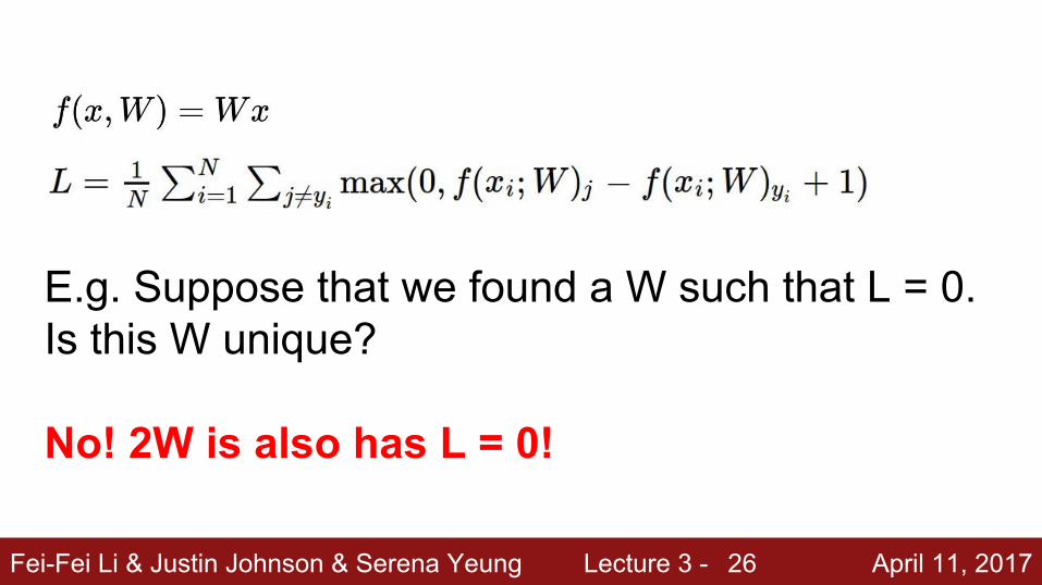
E.g. Suppose that we found a W such that L = 0. Is this W unique?
Fei-Fei Li & Justin Johnson & Serena Yeung Lecture 3 - April 11, 201726
E.g. Suppose that we found a W such that L = 0. Is this W unique?
No! 2W is also has L = 0!

Fei-Fei Li & Justin Johnson & Serena Yeung Lecture 3 - April 11, 201727
Suppose: 3 training examples, 3 classes.With some W the scores are:
cat
frog
car
3.25.1-1.7
4.91.3
2.0 -3.12.52.2
= max(0, 1.3 - 4.9 + 1) +max(0, 2.0 - 4.9 + 1)= max(0, -2.6) + max(0, -1.9)= 0 + 0= 0
0Losses: 2.9
Before:
With W twice as large:= max(0, 2.6 - 9.8 + 1) +max(0, 4.0 - 9.8 + 1)= max(0, -6.2) + max(0, -4.8)= 0 + 0= 0

Fei-Fei Li & Justin Johnson & Serena Yeung Lecture 3 - April 11, 201728
Data loss: Model predictions should match training data

Fei-Fei Li & Justin Johnson & Serena Yeung Lecture 3 - April 11, 201729
Data loss: Model predictions should match training data

Fei-Fei Li & Justin Johnson & Serena Yeung Lecture 3 - April 11, 201730
Data loss: Model predictions should match training data

Fei-Fei Li & Justin Johnson & Serena Yeung Lecture 3 - April 11, 201731
Data loss: Model predictions should match training data

Fei-Fei Li & Justin Johnson & Serena Yeung Lecture 3 - April 11, 201732
Data loss: Model predictions should match training data
Regularization: Model should be “simple”, so it works on test data

Fei-Fei Li & Justin Johnson & Serena Yeung Lecture 3 - April 11, 201733
Data loss: Model predictions should match training data
Regularization: Model should be “simple”, so it works on test data
Occam’s Razor: “Among competing hypotheses, the simplest is the best”William of Ockham, 1285 - 1347

Fei-Fei Li & Justin Johnson & Serena Yeung Lecture 3 - April 11, 2017
Regularization
34
= regularization strength(hyperparameter)
In common use: L2 regularizationL1 regularizationElastic net (L1 + L2)Max norm regularization (might see later)Dropout (will see later)Fancier: Batch normalization, stochastic depth

Fei-Fei Li & Justin Johnson & Serena Yeung Lecture 3 - April 11, 2017
L2 Regularization (Weight Decay)
35

Fei-Fei Li & Justin Johnson & Serena Yeung Lecture 3 - April 11, 2017
L2 Regularization (Weight Decay)
36
(If you are a Bayesian: L2 regularization also corresponds MAP inference using a Gaussian prior on W)

Fei-Fei Li & Justin Johnson & Serena Yeung Lecture 3 - April 11, 201737
Softmax Classifier (Multinomial Logistic Regression)
cat
frog
car
3.25.1-1.7

Fei-Fei Li & Justin Johnson & Serena Yeung Lecture 3 - April 11, 201738
Softmax Classifier (Multinomial Logistic Regression)
scores = unnormalized log probabilities of the classes.
cat
frog
car
3.25.1-1.7

Fei-Fei Li & Justin Johnson & Serena Yeung Lecture 3 - April 11, 201739
Softmax Classifier (Multinomial Logistic Regression)
scores = unnormalized log probabilities of the classes.
cat
frog
car
3.25.1-1.7
where

Fei-Fei Li & Justin Johnson & Serena Yeung Lecture 3 - April 11, 201740
Softmax Classifier (Multinomial Logistic Regression)
scores = unnormalized log probabilities of the classes.
cat
frog
car
3.25.1-1.7
where
Softmax function
Fei-Fei Li & Justin Johnson & Serena Yeung Lecture 3 - April 11, 201741
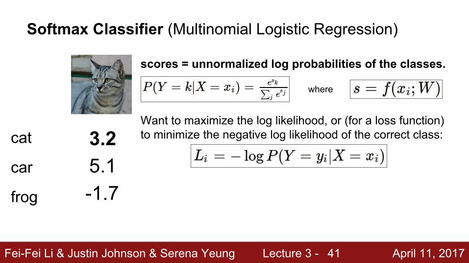
Softmax Classifier (Multinomial Logistic Regression)
scores = unnormalized log probabilities of the classes.
Want to maximize the log likelihood, or (for a loss function) to minimize the negative log likelihood of the correct class:cat
frog
car
3.25.1-1.7
where

Fei-Fei Li & Justin Johnson & Serena Yeung Lecture 3 - April 11, 201742
Softmax Classifier (Multinomial Logistic Regression)
scores = unnormalized log probabilities of the classes.
Want to maximize the log likelihood, or (for a loss function) to minimize the negative log likelihood of the correct class:cat
frog
car
3.25.1-1.7 in summary:
where

Fei-Fei Li & Justin Johnson & Serena Yeung Lecture 3 - April 11, 201743
Softmax Classifier (Multinomial Logistic Regression)
cat
frog
car
3.25.1-1.7
unnormalized log probabilities

Fei-Fei Li & Justin Johnson & Serena Yeung Lecture 3 - April 11, 201744
Softmax Classifier (Multinomial Logistic Regression)
cat
frog
car
3.25.1-1.7
unnormalized log probabilities
24.5164.00.18
exp
unnormalized probabilities

Fei-Fei Li & Justin Johnson & Serena Yeung Lecture 3 - April 11, 201745
Softmax Classifier (Multinomial Logistic Regression)
cat
frog
car
3.25.1-1.7
unnormalized log probabilities
24.5164.00.18
exp
unnormalized probabilities
normalize0.130.870.00
probabilities

Fei-Fei Li & Justin Johnson & Serena Yeung Lecture 3 - April 11, 201746
Softmax Classifier (Multinomial Logistic Regression)
cat
frog
car
3.25.1-1.7
unnormalized log probabilities
24.5164.00.18
exp
unnormalized probabilities
normalize0.130.870.00
probabilities
L_i = -log(0.13) = 0.89

Fei-Fei Li & Justin Johnson & Serena Yeung Lecture 3 - April 11, 201747
Softmax Classifier (Multinomial Logistic Regression)
cat
frog
car
3.25.1-1.7
unnormalized log probabilities
24.5164.00.18
exp normalize
unnormalized probabilities
0.130.870.00
probabilities
L_i = -log(0.13) = 0.89
Q: What is the min/max possible loss L_i?

Fei-Fei Li & Justin Johnson & Serena Yeung Lecture 3 - April 11, 201748
Softmax Classifier (Multinomial Logistic Regression)
cat
frog
car
3.25.1-1.7
unnormalized log probabilities
24.5164.00.18
exp normalize
unnormalized probabilities
0.130.870.00
probabilities
L_i = -log(0.13) = 0.89
Q2: Usually at initialization W is small so all s ≈ 0.What is the loss?
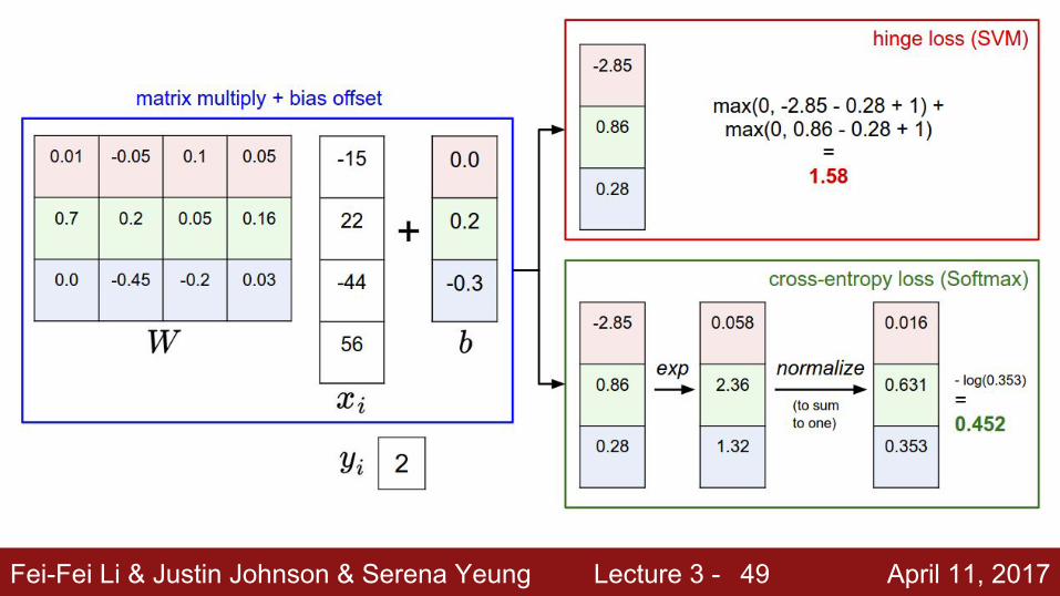
Fei-Fei Li & Justin Johnson & Serena Yeung Lecture 3 - April 11, 201749

Fei-Fei Li & Justin Johnson & Serena Yeung Lecture 3 - April 11, 201750
Softmax vs. SVM

Fei-Fei Li & Justin Johnson & Serena Yeung Lecture 3 - April 11, 201751
Softmax vs. SVM
assume scores:[10, -2, 3][10, 9, 9][10, -100, -100]and
Q: Suppose I take a datapoint and I jiggle a bit (changing its score slightly). What happens to the loss in both cases?

Fei-Fei Li & Justin Johnson & Serena Yeung Lecture 3 - April 11, 201752
Recap- We have some dataset of (x,y)- We have a score function: - We have a loss function:
e.g.
Softmax
SVM
Full loss

Fei-Fei Li & Justin Johnson & Serena Yeung Lecture 3 - April 11, 201753
Recap- We have some dataset of (x,y)- We have a score function: - We have a loss function:
e.g.
Softmax
SVM
Full loss
How do we find the best W?

Fei-Fei Li & Justin Johnson & Serena Yeung Lecture 3 - April 11, 201754
Optimization

Fei-Fei Li & Justin Johnson & Serena Yeung Lecture 3 - April 11, 201755
This image is CC0 1.0 public domain

Fei-Fei Li & Justin Johnson & Serena Yeung Lecture 3 - April 11, 201756Walking man image is CC0 1.0 public domain

Fei-Fei Li & Justin Johnson & Serena Yeung Lecture 3 - April 11, 201757
Strategy #1: A first very bad idea solution: Random search

Fei-Fei Li & Justin Johnson & Serena Yeung Lecture 3 - April 11, 201758
Lets see how well this works on the test set...
15.5% accuracy! not bad!(SOTA is ~95%)

Fei-Fei Li & Justin Johnson & Serena Yeung Lecture 3 - April 11, 201759
Strategy #2: Follow the slope

Fei-Fei Li & Justin Johnson & Serena Yeung Lecture 3 - April 11, 201760
Strategy #2: Follow the slope
In 1-dimension, the derivative of a function:
In multiple dimensions, the gradient is the vector of (partial derivatives) along each dimension
The slope in any direction is the dot product of the direction with the gradientThe direction of steepest descent is the negative gradient

Fei-Fei Li & Justin Johnson & Serena Yeung Lecture 3 - April 11, 201761
current W:
[0.34,-1.11,0.78,0.12,0.55,2.81,-3.1,-1.5,0.33,…] loss 1.25347
gradient dW:
[?,?,?,?,?,?,?,?,?,…]

Fei-Fei Li & Justin Johnson & Serena Yeung Lecture 3 - April 11, 201762
current W:
[0.34,-1.11,0.78,0.12,0.55,2.81,-3.1,-1.5,0.33,…] loss 1.25347
W + h (first dim):
[0.34 + 0.0001,-1.11,0.78,0.12,0.55,2.81,-3.1,-1.5,0.33,…] loss 1.25322
gradient dW:
[?,?,?,?,?,?,?,?,?,…]

Fei-Fei Li & Justin Johnson & Serena Yeung Lecture 3 - April 11, 201763
gradient dW:
[-2.5,?,?,?,?,?,?,?,?,…]
(1.25322 - 1.25347)/0.0001= -2.5
current W:
[0.34,-1.11,0.78,0.12,0.55,2.81,-3.1,-1.5,0.33,…] loss 1.25347
W + h (first dim):
[0.34 + 0.0001,-1.11,0.78,0.12,0.55,2.81,-3.1,-1.5,0.33,…] loss 1.25322

Fei-Fei Li & Justin Johnson & Serena Yeung Lecture 3 - April 11, 201764
gradient dW:
[-2.5,?,?,?,?,?,?,?,?,…]
current W:
[0.34,-1.11,0.78,0.12,0.55,2.81,-3.1,-1.5,0.33,…] loss 1.25347
W + h (second dim):
[0.34,-1.11 + 0.0001,0.78,0.12,0.55,2.81,-3.1,-1.5,0.33,…] loss 1.25353

Fei-Fei Li & Justin Johnson & Serena Yeung Lecture 3 - April 11, 201765
gradient dW:
[-2.5,0.6,?,?,?,?,?,?,?,…]
current W:
[0.34,-1.11,0.78,0.12,0.55,2.81,-3.1,-1.5,0.33,…] loss 1.25347
W + h (second dim):
[0.34,-1.11 + 0.0001,0.78,0.12,0.55,2.81,-3.1,-1.5,0.33,…] loss 1.25353
(1.25353 - 1.25347)/0.0001= 0.6

Fei-Fei Li & Justin Johnson & Serena Yeung Lecture 3 - April 11, 201766
gradient dW:
[-2.5,0.6,?,?,?,?,?,?,?,…]
current W:
[0.34,-1.11,0.78,0.12,0.55,2.81,-3.1,-1.5,0.33,…] loss 1.25347
W + h (third dim):
[0.34,-1.11,0.78 + 0.0001,0.12,0.55,2.81,-3.1,-1.5,0.33,…] loss 1.25347
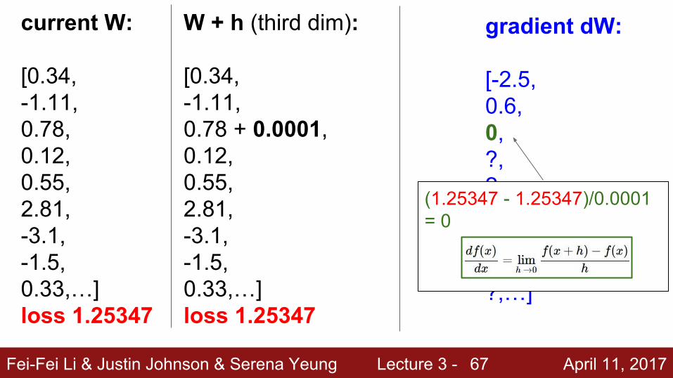
Fei-Fei Li & Justin Johnson & Serena Yeung Lecture 3 - April 11, 201767
gradient dW:
[-2.5,0.6,0,?,?,?,?,?,?,…]
current W:
[0.34,-1.11,0.78,0.12,0.55,2.81,-3.1,-1.5,0.33,…] loss 1.25347
W + h (third dim):
[0.34,-1.11,0.78 + 0.0001,0.12,0.55,2.81,-3.1,-1.5,0.33,…] loss 1.25347
(1.25347 - 1.25347)/0.0001= 0

Fei-Fei Li & Justin Johnson & Serena Yeung Lecture 3 - April 11, 201768
This is silly. The loss is just a function of W:
want

Fei-Fei Li & Justin Johnson & Serena Yeung Lecture 3 - April 11, 201769
This is silly. The loss is just a function of W:
want
This image is in the public domain This image is in the public domain

Fei-Fei Li & Justin Johnson & Serena Yeung Lecture 3 - April 11, 201770
This is silly. The loss is just a function of W:
want
This image is in the public domain This image is in the public domain
Calculus!
Hammer image is in the public domain
Use calculus to compute an analytic gradient

Fei-Fei Li & Justin Johnson & Serena Yeung Lecture 3 - April 11, 201771
gradient dW:
[-2.5,0.6,0,0.2,0.7,-0.5,1.1,1.3,-2.1,…]
current W:
[0.34,-1.11,0.78,0.12,0.55,2.81,-3.1,-1.5,0.33,…] loss 1.25347
dW = ...(some function data and W)

Fei-Fei Li & Justin Johnson & Serena Yeung Lecture 3 - April 11, 201772
In summary:- Numerical gradient: approximate, slow, easy to write
- Analytic gradient: exact, fast, error-prone
=>
In practice: Always use analytic gradient, but check implementation with numerical gradient. This is called a gradient check.

Fei-Fei Li & Justin Johnson & Serena Yeung Lecture 3 - April 11, 201773
Gradient Descent

Fei-Fei Li & Justin Johnson & Serena Yeung Lecture 3 - April 11, 201774
original W
negative gradient directionW_1
W_2

Fei-Fei Li & Justin Johnson & Serena Yeung Lecture 3 - April 11, 201775

Fei-Fei Li & Justin Johnson & Serena Yeung Lecture 3 - April 11, 2017
Stochastic Gradient Descent (SGD)
76
Full sum expensive when N is large!
Approximate sum using a minibatch of examples32 / 64 / 128 common

Fei-Fei Li & Justin Johnson & Serena Yeung Lecture 3 - April 11, 201777
Interactive Web Demo time....
http://vision.stanford.edu/teaching/cs231n-demos/linear-classify/

Fei-Fei Li & Justin Johnson & Serena Yeung Lecture 3 - April 11, 201778
Interactive Web Demo time....

Fei-Fei Li & Justin Johnson & Serena Yeung Lecture 3 - April 11, 2017
Aside: Image Features
79

Fei-Fei Li & Justin Johnson & Serena Yeung Lecture 3 - April 11, 2017
Image Features: Motivation
80
x
y
r
θ
f(x, y) = (r(x, y), θ(x, y))
Cannot separate red and blue points with linear classifier
After applying feature transform, points can be separated by linear classifier

Fei-Fei Li & Justin Johnson & Serena Yeung Lecture 3 - April 11, 2017
Example: Color Histogram
81
+1

Fei-Fei Li & Justin Johnson & Serena Yeung Lecture 3 - April 11, 2017
Example: Histogram of Oriented Gradients (HoG)
82
Divide image into 8x8 pixel regionsWithin each region quantize edge direction into 9 bins
Example: 320x240 image gets divided into 40x30 bins; in each bin there are 9 numbers so feature vector has 30*40*9 = 10,800 numbers
Lowe, “Object recognition from local scale-invariant features”, ICCV 1999Dalal and Triggs, "Histograms of oriented gradients for human detection," CVPR 2005

Fei-Fei Li & Justin Johnson & Serena Yeung Lecture 3 - April 11, 2017
Example: Bag of Words
83
Extract random patches
Cluster patches to form “codebook” of “visual words”
Step 1: Build codebook
Step 2: Encode images
Fei-Fei and Perona, “A bayesian hierarchical model for learning natural scene categories”, CVPR 2005

Fei-Fei Li & Justin Johnson & Serena Yeung Lecture 3 - April 11, 2017
Feature Extraction
Image features vs ConvNets
84
f10 numbers giving scores for classes
training
training
10 numbers giving scores for classes

Fei-Fei Li & Justin Johnson & Serena Yeung Lecture 3 - April 11, 2017
Next time:
Introduction to neural networks
Backpropagation
85