
Lecture 3: Loss functions and...
76
Lecture 3 - 11 Jan 2016 Fei-Fei Li & Andrej Karpathy & Justin Johnson Fei-Fei Li & Andrej Karpathy & Justin Johnson Lecture 3 - 11 Jan 2016 1 Lecture 3: Loss functions and Optimization
Transcript of Lecture 3: Loss functions and...
Lecture 3 - 11 Jan 2016Fei-Fei Li & Andrej Karpathy & Justin JohnsonFei-Fei Li & Andrej Karpathy & Justin Johnson Lecture 3 - 11 Jan 20161
Lecture 3:Loss functions and
Optimization

Lecture 3 - 11 Jan 2016Fei-Fei Li & Andrej Karpathy & Justin JohnsonFei-Fei Li & Andrej Karpathy & Justin Johnson Lecture 3 - 11 Jan 20162
AdministrativeA1 is due Jan 20 (Wednesday). ~9 days leftWarning: Jan 18 (Monday) is Holiday (no class/office hours)
Lecture 3 - 11 Jan 2016Fei-Fei Li & Andrej Karpathy & Justin JohnsonFei-Fei Li & Andrej Karpathy & Justin Johnson Lecture 3 - 11 Jan 20163
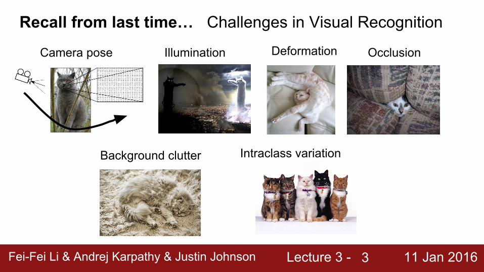
Recall from last time… Challenges in Visual Recognition
Camera pose Illumination Deformation Occlusion
Background clutter Intraclass variation
Lecture 3 - 11 Jan 2016Fei-Fei Li & Andrej Karpathy & Justin JohnsonFei-Fei Li & Andrej Karpathy & Justin Johnson Lecture 3 - 11 Jan 20164
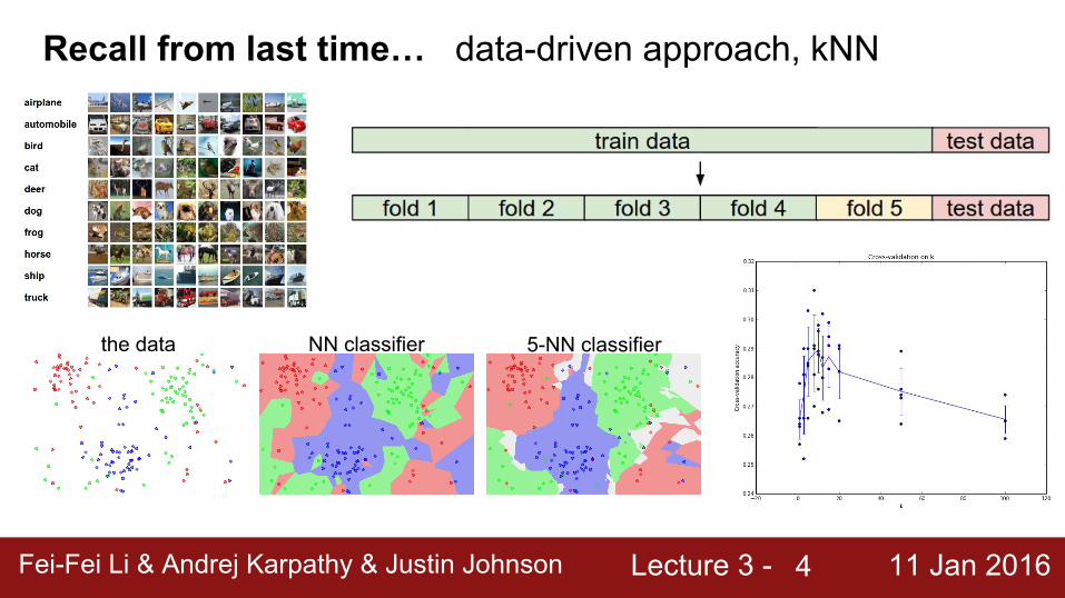
Recall from last time… data-driven approach, kNN
the data NN classifier 5-NN classifier
Lecture 3 - 11 Jan 2016Fei-Fei Li & Andrej Karpathy & Justin JohnsonFei-Fei Li & Andrej Karpathy & Justin Johnson Lecture 3 - 11 Jan 20165
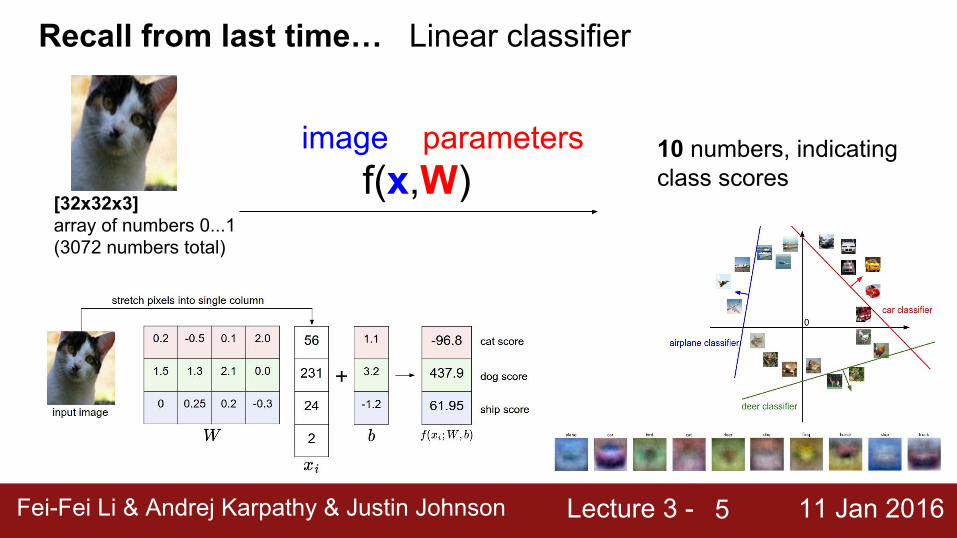
Recall from last time… Linear classifier
[32x32x3]array of numbers 0...1(3072 numbers total)
f(x,W)image parameters 10 numbers, indicating
class scores
Lecture 3 - 11 Jan 2016Fei-Fei Li & Andrej Karpathy & Justin JohnsonFei-Fei Li & Andrej Karpathy & Justin Johnson Lecture 3 - 11 Jan 20166
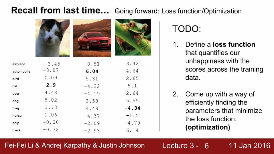
Recall from last time… Going forward: Loss function/Optimization
-3.45-8.870.092.94.488.023.781.06-0.36-0.72
-0.516.045.31-4.22-4.193.584.49-4.37-2.09-2.93
3.424.642.655.12.645.55-4.34-1.5-4.796.14
1. Define a loss function that quantifies our unhappiness with the scores across the training data.
2. Come up with a way of efficiently finding the parameters that minimize the loss function. (optimization)
TODO:
Lecture 3 - 11 Jan 2016Fei-Fei Li & Andrej Karpathy & Justin JohnsonFei-Fei Li & Andrej Karpathy & Justin Johnson Lecture 3 - 11 Jan 20167
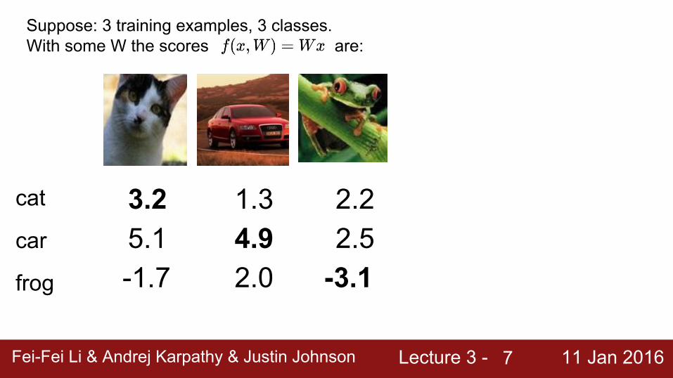
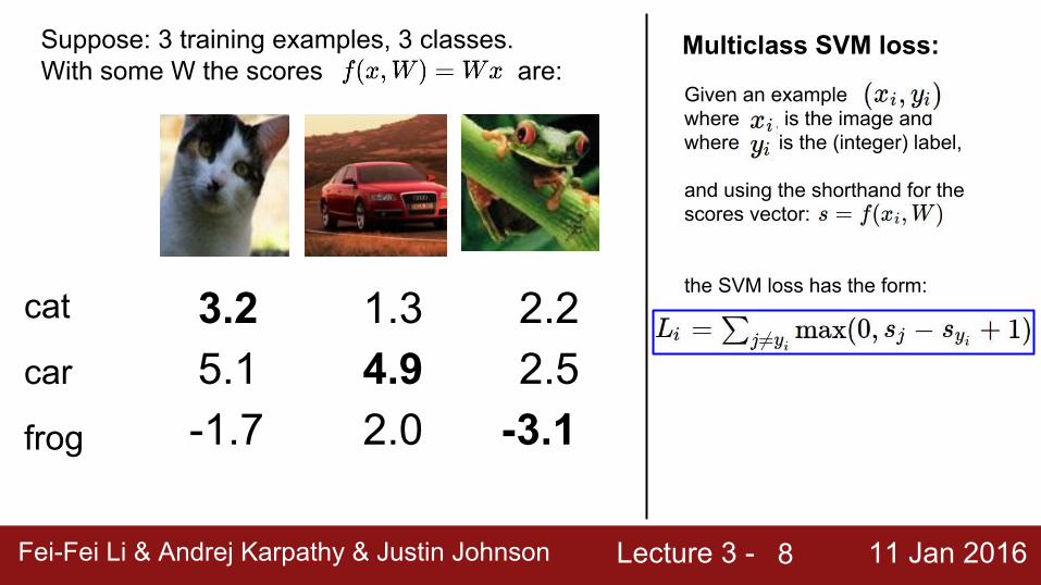
Suppose: 3 training examples, 3 classes.With some W the scores are:
cat
frog
car
3.25.1-1.7
4.91.3
2.0 -3.12.52.2
Lecture 3 - 11 Jan 2016Fei-Fei Li & Andrej Karpathy & Justin JohnsonFei-Fei Li & Andrej Karpathy & Justin Johnson Lecture 3 - 11 Jan 20168
Suppose: 3 training examples, 3 classes.With some W the scores are:
cat
frog
car
3.25.1-1.7
4.91.3
2.0 -3.12.52.2
Multiclass SVM loss:
Given an examplewhere is the image andwhere is the (integer) label,
and using the shorthand for the scores vector:
the SVM loss has the form:
Lecture 3 - 11 Jan 2016Fei-Fei Li & Andrej Karpathy & Justin JohnsonFei-Fei Li & Andrej Karpathy & Justin Johnson Lecture 3 - 11 Jan 20169
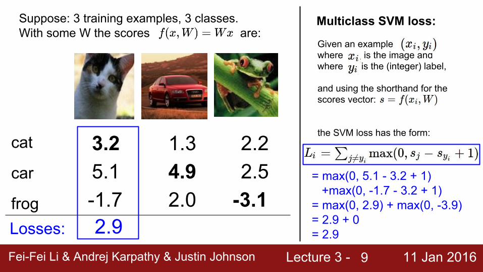
Suppose: 3 training examples, 3 classes.With some W the scores are:
cat
frog
car
3.25.1-1.7
4.91.3
2.0 -3.12.52.2
Multiclass SVM loss:
Given an examplewhere is the image andwhere is the (integer) label,
and using the shorthand for the scores vector:
the SVM loss has the form:
= max(0, 5.1 - 3.2 + 1) +max(0, -1.7 - 3.2 + 1)= max(0, 2.9) + max(0, -3.9)= 2.9 + 0= 2.92.9Losses:
Lecture 3 - 11 Jan 2016Fei-Fei Li & Andrej Karpathy & Justin JohnsonFei-Fei Li & Andrej Karpathy & Justin Johnson Lecture 3 - 11 Jan 201610
Suppose: 3 training examples, 3 classes.With some W the scores are:
cat
frog
car
3.25.1-1.7
4.91.3
2.0 -3.12.52.2
Multiclass SVM loss:
Given an examplewhere is the image andwhere is the (integer) label,
and using the shorthand for the scores vector:
the SVM loss has the form:
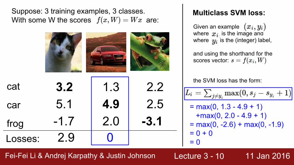
= max(0, 1.3 - 4.9 + 1) +max(0, 2.0 - 4.9 + 1)= max(0, -2.6) + max(0, -1.9)= 0 + 0= 00Losses: 2.9
Lecture 3 - 11 Jan 2016Fei-Fei Li & Andrej Karpathy & Justin JohnsonFei-Fei Li & Andrej Karpathy & Justin Johnson Lecture 3 - 11 Jan 201611
Suppose: 3 training examples, 3 classes.With some W the scores are:
cat
frog
car
3.25.1-1.7
4.91.3
2.0 -3.12.52.2
Multiclass SVM loss:
Given an examplewhere is the image andwhere is the (integer) label,
and using the shorthand for the scores vector:
the SVM loss has the form:
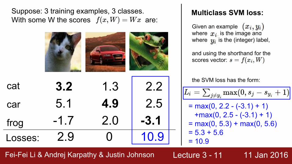
= max(0, 2.2 - (-3.1) + 1) +max(0, 2.5 - (-3.1) + 1)= max(0, 5.3) + max(0, 5.6)= 5.3 + 5.6= 10.90Losses: 2.9 10.9
Lecture 3 - 11 Jan 2016Fei-Fei Li & Andrej Karpathy & Justin JohnsonFei-Fei Li & Andrej Karpathy & Justin Johnson Lecture 3 - 11 Jan 201612
cat
frog
car
3.25.1-1.7
4.91.3
2.0 -3.12.52.2
0Losses: 2.9 10.9
Suppose: 3 training examples, 3 classes.With some W the scores are:
Multiclass SVM loss:
Given an examplewhere is the image andwhere is the (integer) label,
and using the shorthand for the scores vector:
the SVM loss has the form:
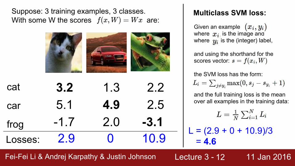
and the full training loss is the mean over all examples in the training data:
L = (2.9 + 0 + 10.9)/3 = 4.6
Lecture 3 - 11 Jan 2016Fei-Fei Li & Andrej Karpathy & Justin JohnsonFei-Fei Li & Andrej Karpathy & Justin Johnson Lecture 3 - 11 Jan 201613
cat
frog
car
3.25.1-1.7
4.91.3
2.0 -3.12.52.2
0Losses: 2.9 10.9
Suppose: 3 training examples, 3 classes.With some W the scores are:
Multiclass SVM loss:
Given an examplewhere is the image andwhere is the (integer) label,
and using the shorthand for the scores vector:
the SVM loss has the form:
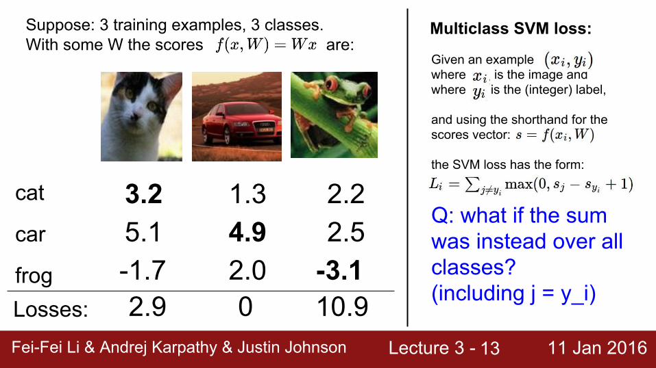
Q: what if the sum was instead over all classes? (including j = y_i)
Lecture 3 - 11 Jan 2016Fei-Fei Li & Andrej Karpathy & Justin JohnsonFei-Fei Li & Andrej Karpathy & Justin Johnson Lecture 3 - 11 Jan 201614
cat
frog
car
3.25.1-1.7
4.91.3
2.0 -3.12.52.2
0Losses: 2.9 10.9
Suppose: 3 training examples, 3 classes.With some W the scores are:
Multiclass SVM loss:
Given an examplewhere is the image andwhere is the (integer) label,
and using the shorthand for the scores vector:
the SVM loss has the form:
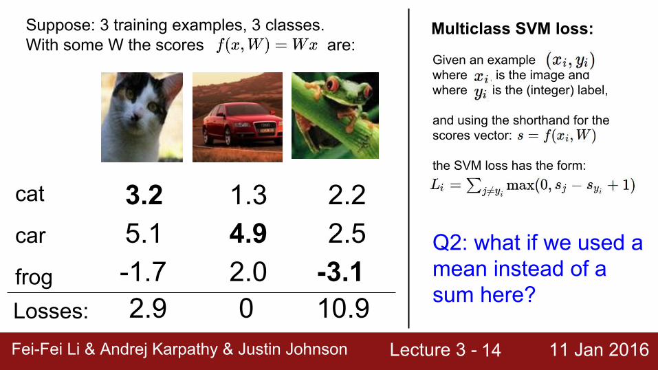
Q2: what if we used a mean instead of a sum here?
Lecture 3 - 11 Jan 2016Fei-Fei Li & Andrej Karpathy & Justin JohnsonFei-Fei Li & Andrej Karpathy & Justin Johnson Lecture 3 - 11 Jan 201615
cat
frog
car
3.25.1-1.7
4.91.3
2.0 -3.12.52.2
0Losses: 2.9 10.9
Suppose: 3 training examples, 3 classes.With some W the scores are:
Multiclass SVM loss:
Given an examplewhere is the image andwhere is the (integer) label,
and using the shorthand for the scores vector:
the SVM loss has the form:
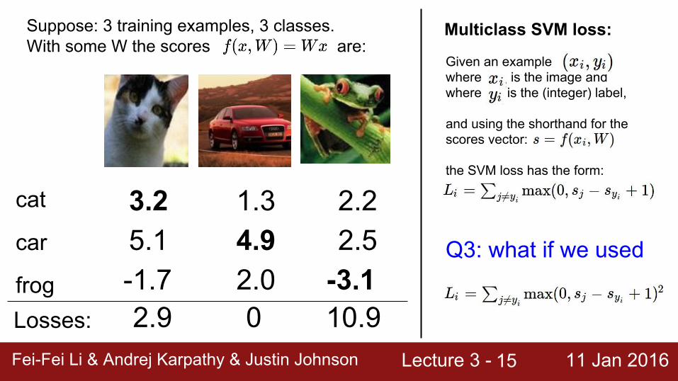
Q3: what if we used

Lecture 3 - 11 Jan 2016Fei-Fei Li & Andrej Karpathy & Justin JohnsonFei-Fei Li & Andrej Karpathy & Justin Johnson Lecture 3 - 11 Jan 201616
cat
frog
car
3.25.1-1.7
4.91.3
2.0 -3.12.52.2
0Losses: 2.9 10.9
Suppose: 3 training examples, 3 classes.With some W the scores are:
Multiclass SVM loss:
Given an examplewhere is the image andwhere is the (integer) label,
and using the shorthand for the scores vector:
the SVM loss has the form:
Q4: what is the min/max possible loss?
Lecture 3 - 11 Jan 2016Fei-Fei Li & Andrej Karpathy & Justin JohnsonFei-Fei Li & Andrej Karpathy & Justin Johnson Lecture 3 - 11 Jan 201617
cat
frog
car
3.25.1-1.7
4.91.3
2.0 -3.12.52.2
0Losses: 2.9 10.9
Suppose: 3 training examples, 3 classes.With some W the scores are:
Multiclass SVM loss:
Given an examplewhere is the image andwhere is the (integer) label,
and using the shorthand for the scores vector:
the SVM loss has the form:
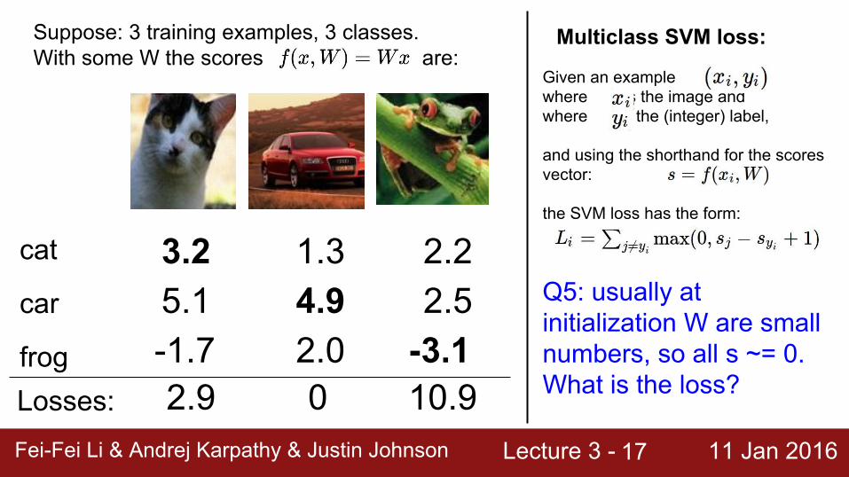
Q5: usually at initialization W are small numbers, so all s ~= 0. What is the loss?
Lecture 3 - 11 Jan 2016Fei-Fei Li & Andrej Karpathy & Justin JohnsonFei-Fei Li & Andrej Karpathy & Justin Johnson Lecture 3 - 11 Jan 201618
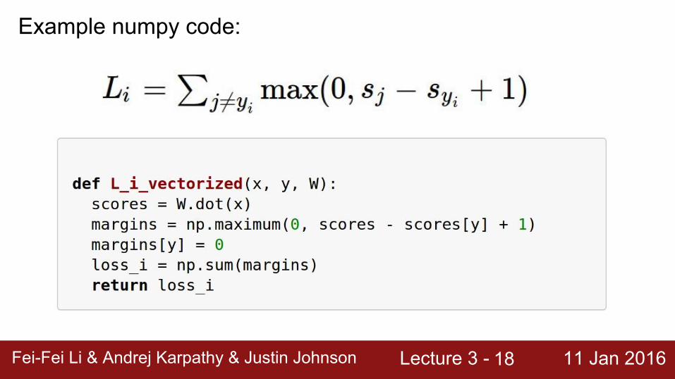
Example numpy code:
Lecture 3 - 11 Jan 2016Fei-Fei Li & Andrej Karpathy & Justin JohnsonFei-Fei Li & Andrej Karpathy & Justin Johnson Lecture 3 - 11 Jan 201619
Lecture 3 - 11 Jan 2016Fei-Fei Li & Andrej Karpathy & Justin JohnsonFei-Fei Li & Andrej Karpathy & Justin Johnson Lecture 3 - 11 Jan 201620
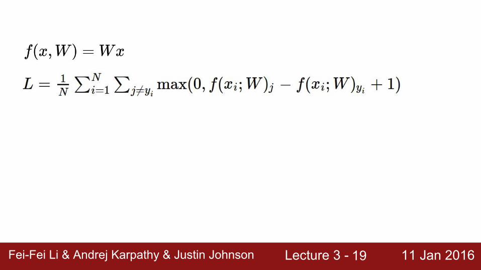
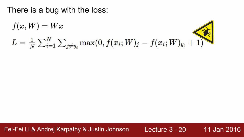
There is a bug with the loss:
Lecture 3 - 11 Jan 2016Fei-Fei Li & Andrej Karpathy & Justin JohnsonFei-Fei Li & Andrej Karpathy & Justin Johnson Lecture 3 - 11 Jan 201621
There is a bug with the loss:
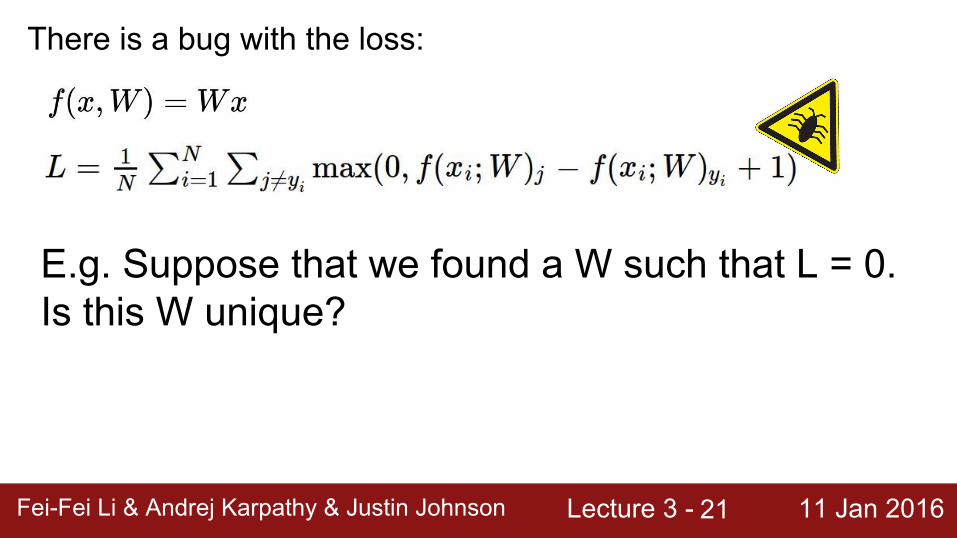
E.g. Suppose that we found a W such that L = 0. Is this W unique?
Lecture 3 - 11 Jan 2016Fei-Fei Li & Andrej Karpathy & Justin JohnsonFei-Fei Li & Andrej Karpathy & Justin Johnson Lecture 3 - 11 Jan 201622
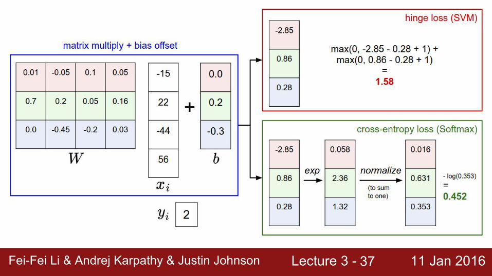
Suppose: 3 training examples, 3 classes.With some W the scores are:
cat
frog
car
3.25.1-1.7
4.91.3
2.0 -3.12.52.2
= max(0, 1.3 - 4.9 + 1) +max(0, 2.0 - 4.9 + 1)= max(0, -2.6) + max(0, -1.9)= 0 + 0= 0
0Losses: 2.9
Before:
With W twice as large:= max(0, 2.6 - 9.8 + 1) +max(0, 4.0 - 9.8 + 1)= max(0, -6.2) + max(0, -4.8)= 0 + 0= 0
Lecture 3 - 11 Jan 2016Fei-Fei Li & Andrej Karpathy & Justin JohnsonFei-Fei Li & Andrej Karpathy & Justin Johnson Lecture 3 - 11 Jan 201623
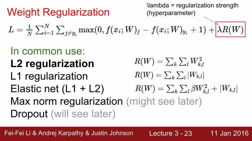
Weight Regularization\lambda = regularization strength(hyperparameter)
In common use: L2 regularizationL1 regularizationElastic net (L1 + L2)Max norm regularization (might see later)Dropout (will see later)
Lecture 3 - 11 Jan 2016Fei-Fei Li & Andrej Karpathy & Justin JohnsonFei-Fei Li & Andrej Karpathy & Justin Johnson Lecture 3 - 11 Jan 201624
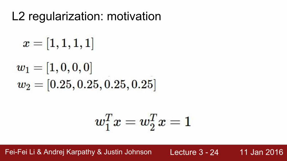
L2 regularization: motivation
Lecture 3 - 11 Jan 2016Fei-Fei Li & Andrej Karpathy & Justin JohnsonFei-Fei Li & Andrej Karpathy & Justin Johnson Lecture 3 - 11 Jan 201625
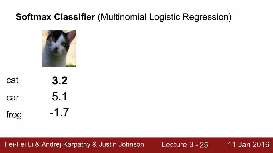
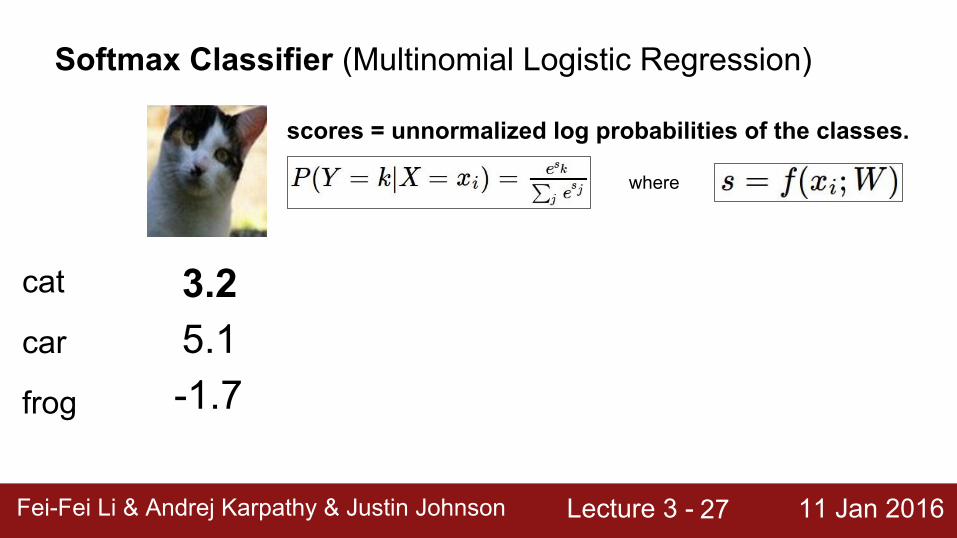
Softmax Classifier (Multinomial Logistic Regression)
cat
frog
car
3.25.1-1.7
Lecture 3 - 11 Jan 2016Fei-Fei Li & Andrej Karpathy & Justin JohnsonFei-Fei Li & Andrej Karpathy & Justin Johnson Lecture 3 - 11 Jan 201626
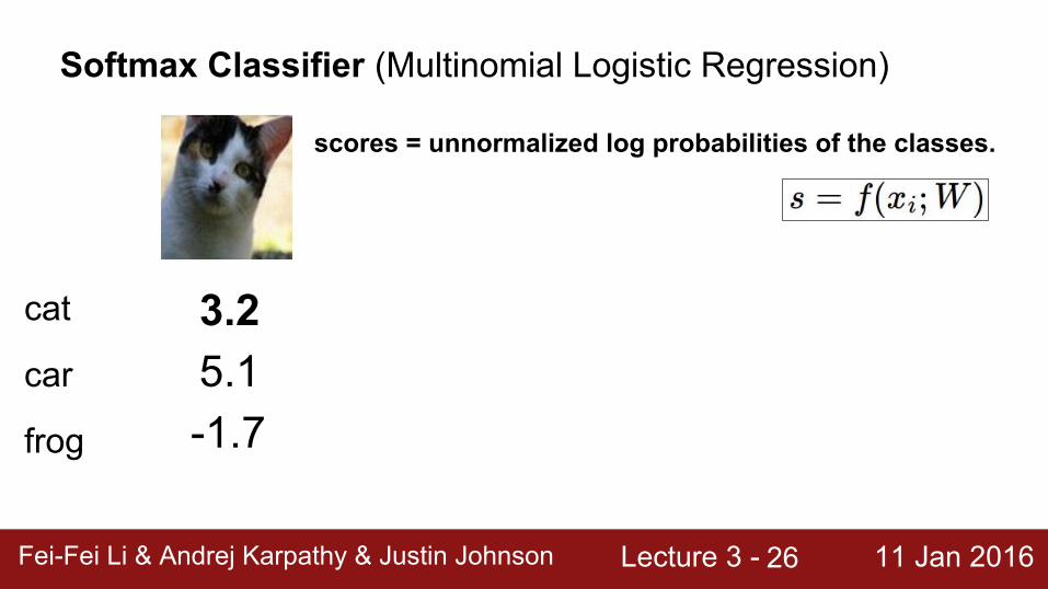
Softmax Classifier (Multinomial Logistic Regression)
scores = unnormalized log probabilities of the classes.
cat
frog
car
3.25.1-1.7
Lecture 3 - 11 Jan 2016Fei-Fei Li & Andrej Karpathy & Justin JohnsonFei-Fei Li & Andrej Karpathy & Justin Johnson Lecture 3 - 11 Jan 201627
Softmax Classifier (Multinomial Logistic Regression)
scores = unnormalized log probabilities of the classes.
cat
frog
car
3.25.1-1.7
where
Lecture 3 - 11 Jan 2016Fei-Fei Li & Andrej Karpathy & Justin JohnsonFei-Fei Li & Andrej Karpathy & Justin Johnson Lecture 3 - 11 Jan 201628
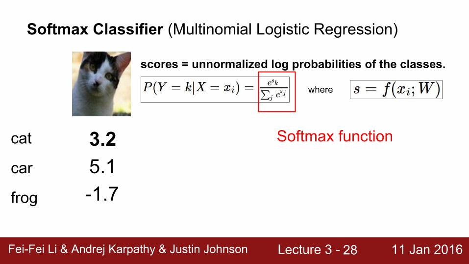
Softmax Classifier (Multinomial Logistic Regression)
scores = unnormalized log probabilities of the classes.
cat
frog
car
3.25.1-1.7
where
Softmax function
Lecture 3 - 11 Jan 2016Fei-Fei Li & Andrej Karpathy & Justin JohnsonFei-Fei Li & Andrej Karpathy & Justin Johnson Lecture 3 - 11 Jan 201629
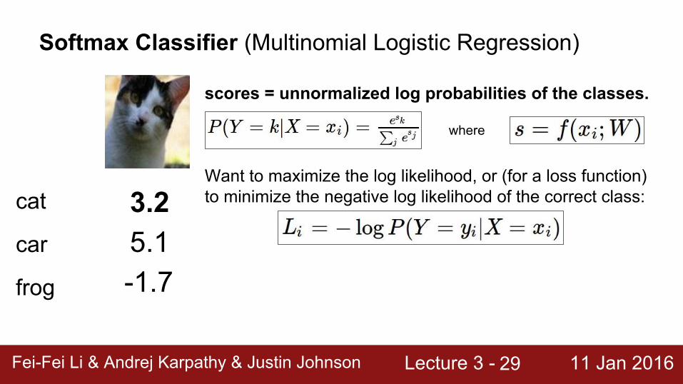
Softmax Classifier (Multinomial Logistic Regression)
scores = unnormalized log probabilities of the classes.
Want to maximize the log likelihood, or (for a loss function) to minimize the negative log likelihood of the correct class:cat
frog
car
3.25.1-1.7
where
Lecture 3 - 11 Jan 2016Fei-Fei Li & Andrej Karpathy & Justin JohnsonFei-Fei Li & Andrej Karpathy & Justin Johnson Lecture 3 - 11 Jan 201630
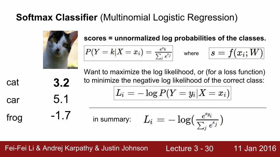
Softmax Classifier (Multinomial Logistic Regression)
scores = unnormalized log probabilities of the classes.
Want to maximize the log likelihood, or (for a loss function) to minimize the negative log likelihood of the correct class:cat
frog
car
3.25.1-1.7 in summary:
where
Lecture 3 - 11 Jan 2016Fei-Fei Li & Andrej Karpathy & Justin JohnsonFei-Fei Li & Andrej Karpathy & Justin Johnson Lecture 3 - 11 Jan 201631
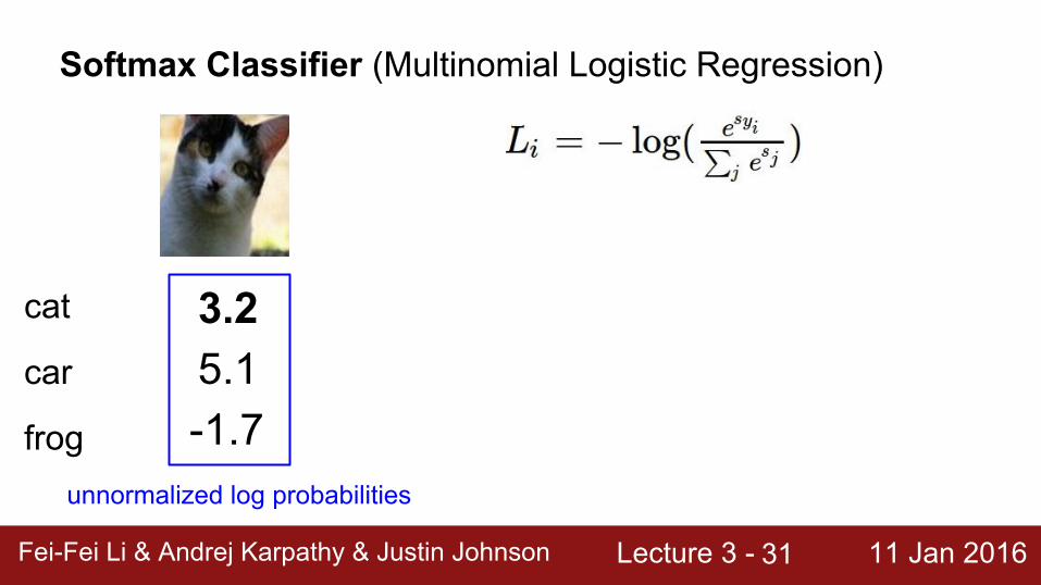
Softmax Classifier (Multinomial Logistic Regression)
cat
frog
car
3.25.1-1.7
unnormalized log probabilities
Lecture 3 - 11 Jan 2016Fei-Fei Li & Andrej Karpathy & Justin JohnsonFei-Fei Li & Andrej Karpathy & Justin Johnson Lecture 3 - 11 Jan 201632
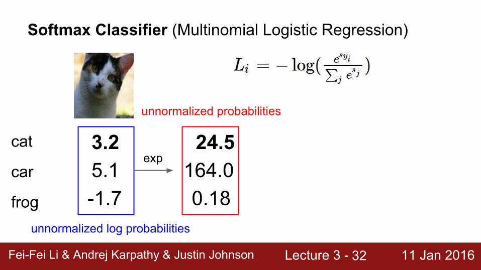
Softmax Classifier (Multinomial Logistic Regression)
cat
frog
car
3.25.1-1.7
unnormalized log probabilities
24.5164.00.18
exp
unnormalized probabilities
Lecture 3 - 11 Jan 2016Fei-Fei Li & Andrej Karpathy & Justin JohnsonFei-Fei Li & Andrej Karpathy & Justin Johnson Lecture 3 - 11 Jan 201633
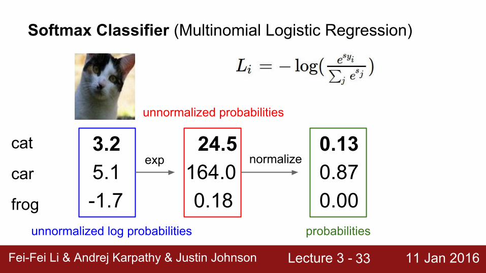
Softmax Classifier (Multinomial Logistic Regression)
cat
frog
car
3.25.1-1.7
unnormalized log probabilities
24.5164.00.18
exp normalize
unnormalized probabilities
0.130.870.00
probabilities
Lecture 3 - 11 Jan 2016Fei-Fei Li & Andrej Karpathy & Justin JohnsonFei-Fei Li & Andrej Karpathy & Justin Johnson Lecture 3 - 11 Jan 201634
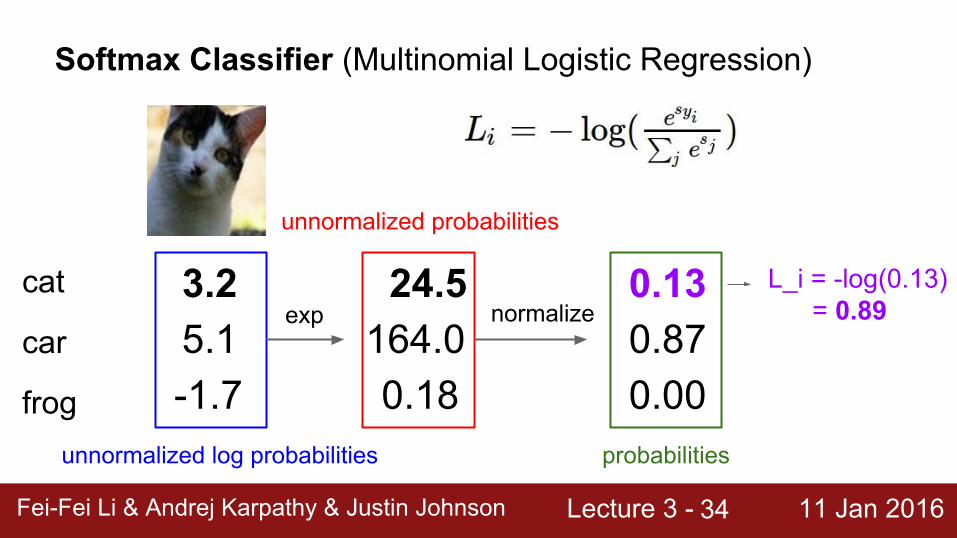
Softmax Classifier (Multinomial Logistic Regression)
cat
frog
car
3.25.1-1.7
unnormalized log probabilities
24.5164.00.18
exp normalize
unnormalized probabilities
0.130.870.00
probabilities
L_i = -log(0.13) = 0.89
Lecture 3 - 11 Jan 2016Fei-Fei Li & Andrej Karpathy & Justin JohnsonFei-Fei Li & Andrej Karpathy & Justin Johnson Lecture 3 - 11 Jan 201635
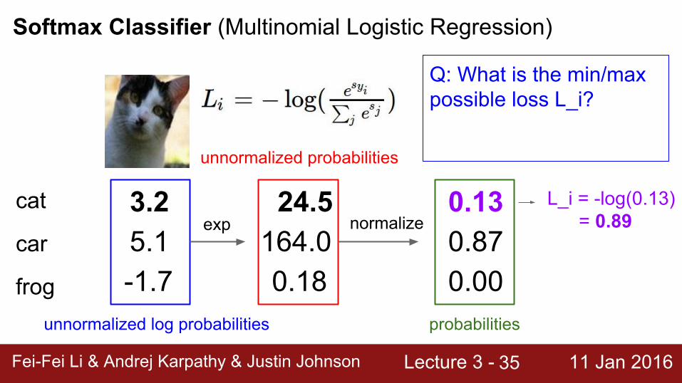
Softmax Classifier (Multinomial Logistic Regression)
cat
frog
car
3.25.1-1.7
unnormalized log probabilities
24.5164.00.18
exp normalize
unnormalized probabilities
0.130.870.00
probabilities
L_i = -log(0.13) = 0.89
Q: What is the min/max possible loss L_i?
Lecture 3 - 11 Jan 2016Fei-Fei Li & Andrej Karpathy & Justin JohnsonFei-Fei Li & Andrej Karpathy & Justin Johnson Lecture 3 - 11 Jan 201636
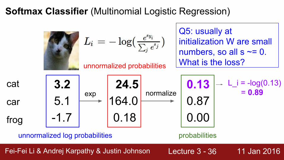
Softmax Classifier (Multinomial Logistic Regression)
cat
frog
car
3.25.1-1.7
unnormalized log probabilities
24.5164.00.18
exp normalize
unnormalized probabilities
0.130.870.00
probabilities
L_i = -log(0.13) = 0.89
Q5: usually at initialization W are small numbers, so all s ~= 0. What is the loss?
Lecture 3 - 11 Jan 2016Fei-Fei Li & Andrej Karpathy & Justin JohnsonFei-Fei Li & Andrej Karpathy & Justin Johnson Lecture 3 - 11 Jan 201637
Lecture 3 - 11 Jan 2016Fei-Fei Li & Andrej Karpathy & Justin JohnsonFei-Fei Li & Andrej Karpathy & Justin Johnson Lecture 3 - 11 Jan 201638
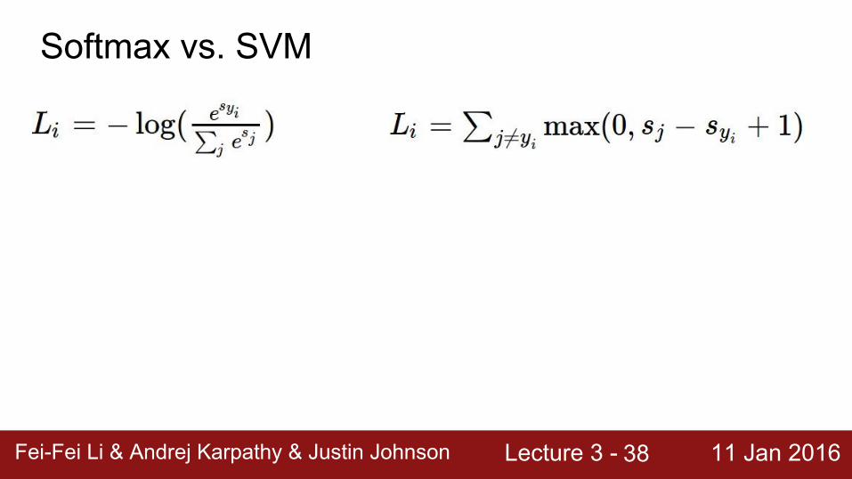
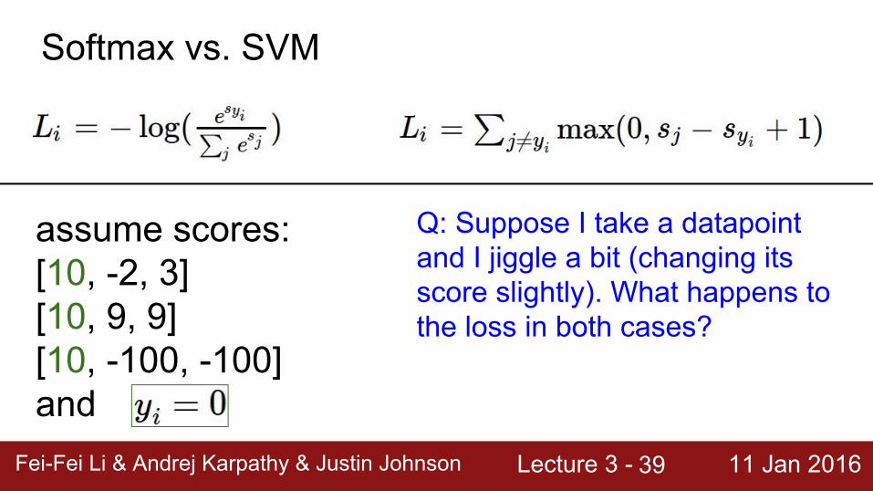
Softmax vs. SVM
Lecture 3 - 11 Jan 2016Fei-Fei Li & Andrej Karpathy & Justin JohnsonFei-Fei Li & Andrej Karpathy & Justin Johnson Lecture 3 - 11 Jan 201639
Softmax vs. SVM
assume scores:[10, -2, 3][10, 9, 9][10, -100, -100]and
Q: Suppose I take a datapoint and I jiggle a bit (changing its score slightly). What happens to the loss in both cases?
Lecture 3 - 11 Jan 2016Fei-Fei Li & Andrej Karpathy & Justin JohnsonFei-Fei Li & Andrej Karpathy & Justin Johnson Lecture 3 - 11 Jan 201640
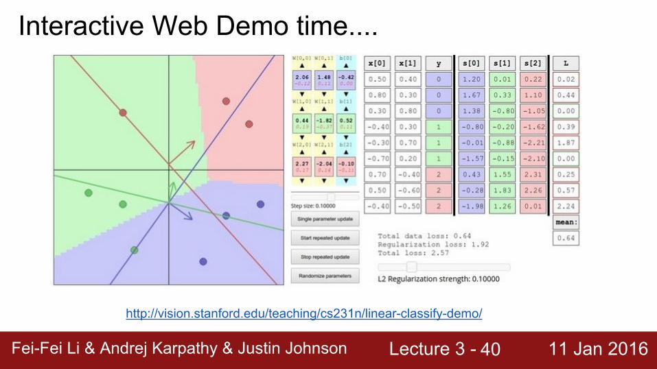
Interactive Web Demo time....
http://vision.stanford.edu/teaching/cs231n/linear-classify-demo/

Lecture 3 - 11 Jan 2016Fei-Fei Li & Andrej Karpathy & Justin JohnsonFei-Fei Li & Andrej Karpathy & Justin Johnson Lecture 3 - 11 Jan 201641
Optimization
Lecture 3 - 11 Jan 2016Fei-Fei Li & Andrej Karpathy & Justin JohnsonFei-Fei Li & Andrej Karpathy & Justin Johnson Lecture 3 - 11 Jan 201642
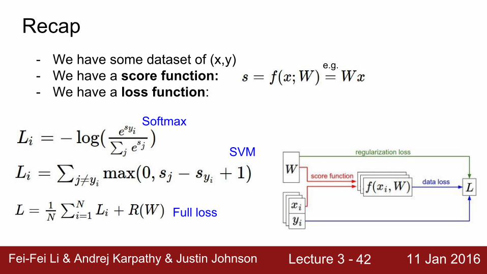
Recap- We have some dataset of (x,y)- We have a score function: - We have a loss function:
e.g.
Softmax
SVM
Full loss
Lecture 3 - 11 Jan 2016Fei-Fei Li & Andrej Karpathy & Justin JohnsonFei-Fei Li & Andrej Karpathy & Justin Johnson Lecture 3 - 11 Jan 201643
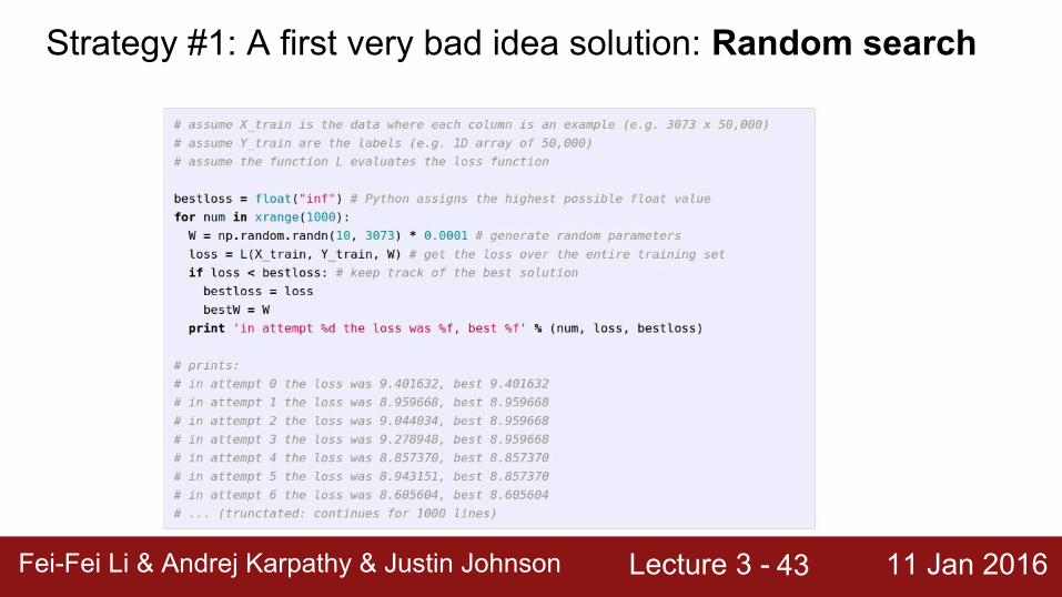
Strategy #1: A first very bad idea solution: Random search
Lecture 3 - 11 Jan 2016Fei-Fei Li & Andrej Karpathy & Justin JohnsonFei-Fei Li & Andrej Karpathy & Justin Johnson Lecture 3 - 11 Jan 201644
Lets see how well this works on the test set...
15.5% accuracy! not bad!(SOTA is ~95%)
Lecture 3 - 11 Jan 2016Fei-Fei Li & Andrej Karpathy & Justin JohnsonFei-Fei Li & Andrej Karpathy & Justin Johnson Lecture 3 - 11 Jan 201645
Lecture 3 - 11 Jan 2016Fei-Fei Li & Andrej Karpathy & Justin JohnsonFei-Fei Li & Andrej Karpathy & Justin Johnson Lecture 3 - 11 Jan 201646
Lecture 3 - 11 Jan 2016Fei-Fei Li & Andrej Karpathy & Justin JohnsonFei-Fei Li & Andrej Karpathy & Justin Johnson Lecture 3 - 11 Jan 201647
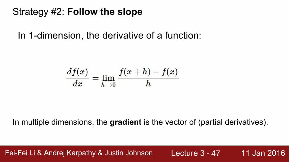
Strategy #2: Follow the slope
In 1-dimension, the derivative of a function:
In multiple dimensions, the gradient is the vector of (partial derivatives).
Lecture 3 - 11 Jan 2016Fei-Fei Li & Andrej Karpathy & Justin JohnsonFei-Fei Li & Andrej Karpathy & Justin Johnson Lecture 3 - 11 Jan 201648
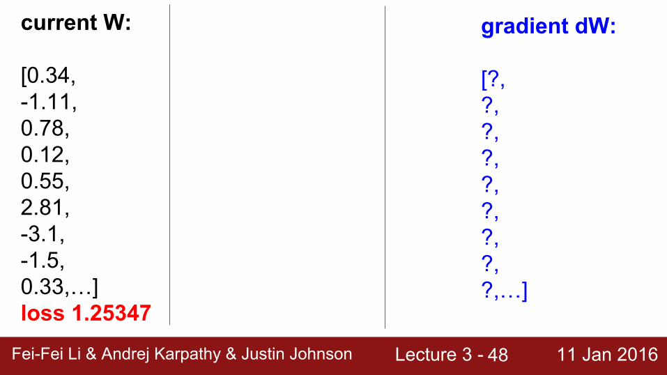
current W:
[0.34,-1.11,0.78,0.12,0.55,2.81,-3.1,-1.5,0.33,…] loss 1.25347
gradient dW:
[?,?,?,?,?,?,?,?,?,…]
Lecture 3 - 11 Jan 2016Fei-Fei Li & Andrej Karpathy & Justin JohnsonFei-Fei Li & Andrej Karpathy & Justin Johnson Lecture 3 - 11 Jan 201649
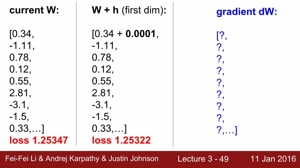
current W:
[0.34,-1.11,0.78,0.12,0.55,2.81,-3.1,-1.5,0.33,…] loss 1.25347
W + h (first dim):
[0.34 + 0.0001,-1.11,0.78,0.12,0.55,2.81,-3.1,-1.5,0.33,…] loss 1.25322
gradient dW:
[?,?,?,?,?,?,?,?,?,…]
Lecture 3 - 11 Jan 2016Fei-Fei Li & Andrej Karpathy & Justin JohnsonFei-Fei Li & Andrej Karpathy & Justin Johnson Lecture 3 - 11 Jan 201650
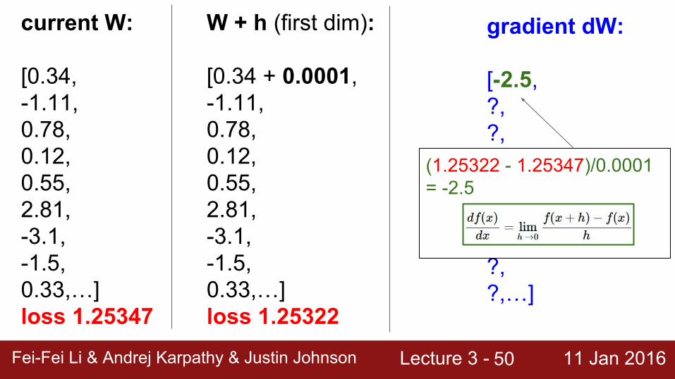
gradient dW:
[-2.5,?,?,?,?,?,?,?,?,…]
(1.25322 - 1.25347)/0.0001= -2.5
current W:
[0.34,-1.11,0.78,0.12,0.55,2.81,-3.1,-1.5,0.33,…] loss 1.25347
W + h (first dim):
[0.34 + 0.0001,-1.11,0.78,0.12,0.55,2.81,-3.1,-1.5,0.33,…] loss 1.25322
Lecture 3 - 11 Jan 2016Fei-Fei Li & Andrej Karpathy & Justin JohnsonFei-Fei Li & Andrej Karpathy & Justin Johnson Lecture 3 - 11 Jan 201651
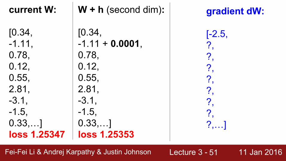
gradient dW:
[-2.5,?,?,?,?,?,?,?,?,…]
current W:
[0.34,-1.11,0.78,0.12,0.55,2.81,-3.1,-1.5,0.33,…] loss 1.25347
W + h (second dim):
[0.34,-1.11 + 0.0001,0.78,0.12,0.55,2.81,-3.1,-1.5,0.33,…] loss 1.25353
Lecture 3 - 11 Jan 2016Fei-Fei Li & Andrej Karpathy & Justin JohnsonFei-Fei Li & Andrej Karpathy & Justin Johnson Lecture 3 - 11 Jan 201652
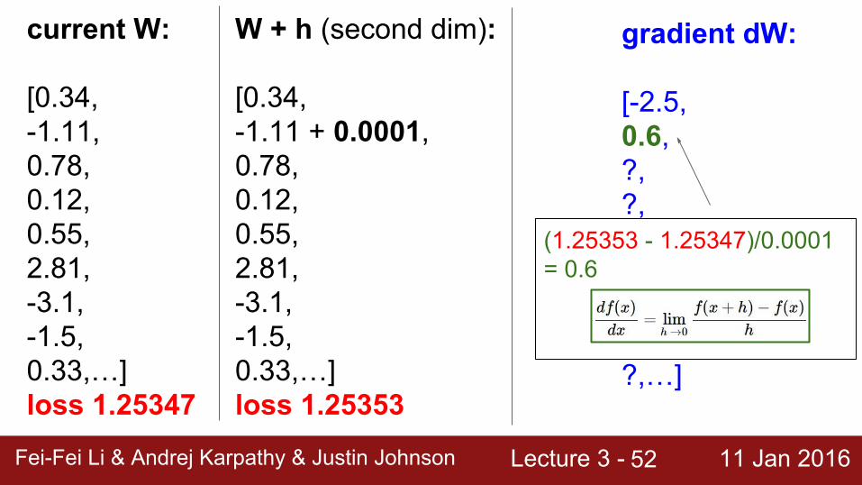
gradient dW:
[-2.5,0.6,?,?,?,?,?,?,?,…]
current W:
[0.34,-1.11,0.78,0.12,0.55,2.81,-3.1,-1.5,0.33,…] loss 1.25347
W + h (second dim):
[0.34,-1.11 + 0.0001,0.78,0.12,0.55,2.81,-3.1,-1.5,0.33,…] loss 1.25353
(1.25353 - 1.25347)/0.0001= 0.6
Lecture 3 - 11 Jan 2016Fei-Fei Li & Andrej Karpathy & Justin JohnsonFei-Fei Li & Andrej Karpathy & Justin Johnson Lecture 3 - 11 Jan 201653
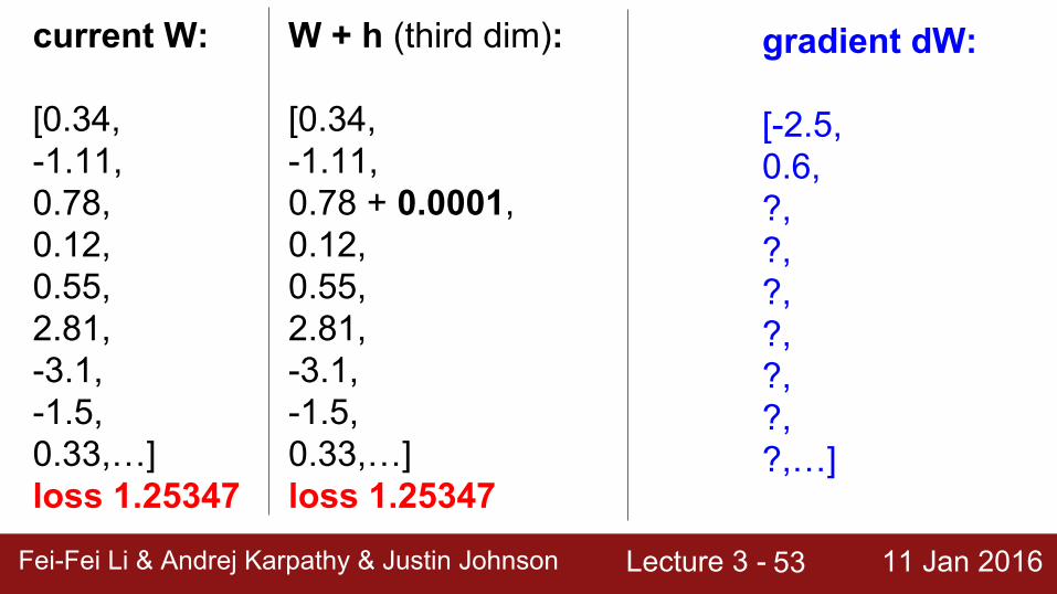
gradient dW:
[-2.5,0.6,?,?,?,?,?,?,?,…]
current W:
[0.34,-1.11,0.78,0.12,0.55,2.81,-3.1,-1.5,0.33,…] loss 1.25347
W + h (third dim):
[0.34,-1.11,0.78 + 0.0001,0.12,0.55,2.81,-3.1,-1.5,0.33,…] loss 1.25347
Lecture 3 - 11 Jan 2016Fei-Fei Li & Andrej Karpathy & Justin JohnsonFei-Fei Li & Andrej Karpathy & Justin Johnson Lecture 3 - 11 Jan 201654
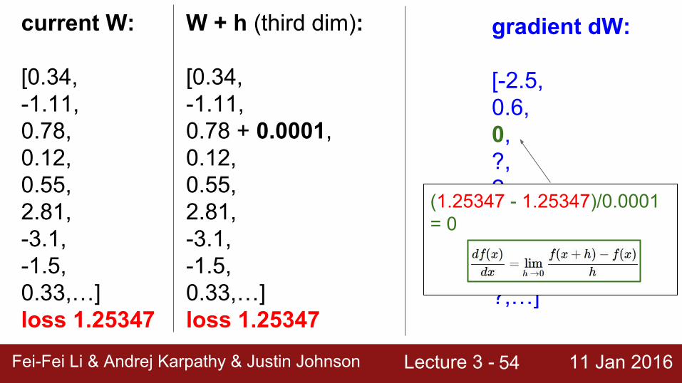
gradient dW:
[-2.5,0.6,0,?,?,?,?,?,?,…]
current W:
[0.34,-1.11,0.78,0.12,0.55,2.81,-3.1,-1.5,0.33,…] loss 1.25347
W + h (third dim):
[0.34,-1.11,0.78 + 0.0001,0.12,0.55,2.81,-3.1,-1.5,0.33,…] loss 1.25347
(1.25347 - 1.25347)/0.0001= 0
Lecture 3 - 11 Jan 2016Fei-Fei Li & Andrej Karpathy & Justin JohnsonFei-Fei Li & Andrej Karpathy & Justin Johnson Lecture 3 - 11 Jan 201655
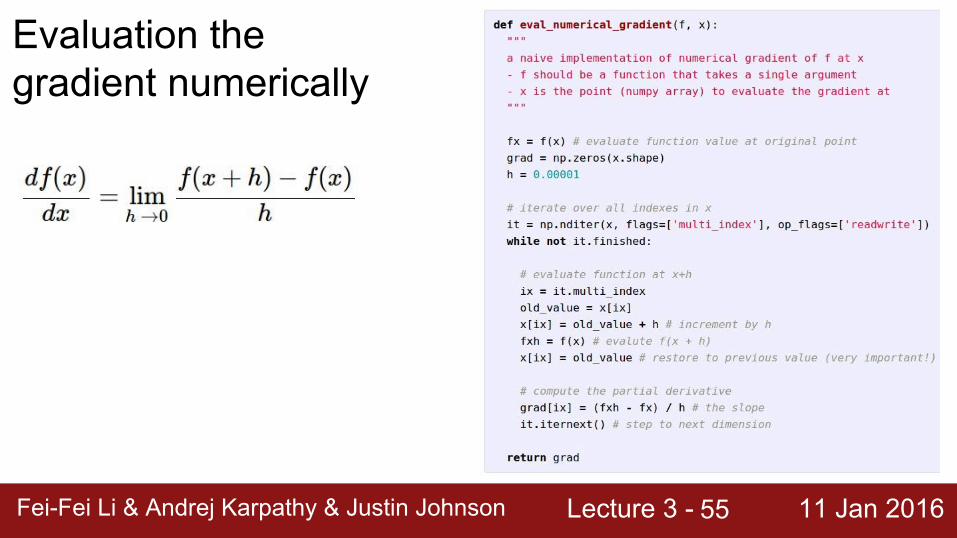
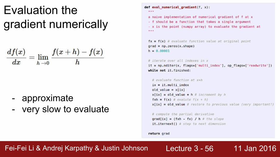
Evaluation the gradient numerically
Lecture 3 - 11 Jan 2016Fei-Fei Li & Andrej Karpathy & Justin JohnsonFei-Fei Li & Andrej Karpathy & Justin Johnson Lecture 3 - 11 Jan 201656
Evaluation the gradient numerically
- approximate- very slow to evaluate
Lecture 3 - 11 Jan 2016Fei-Fei Li & Andrej Karpathy & Justin JohnsonFei-Fei Li & Andrej Karpathy & Justin Johnson Lecture 3 - 11 Jan 201657
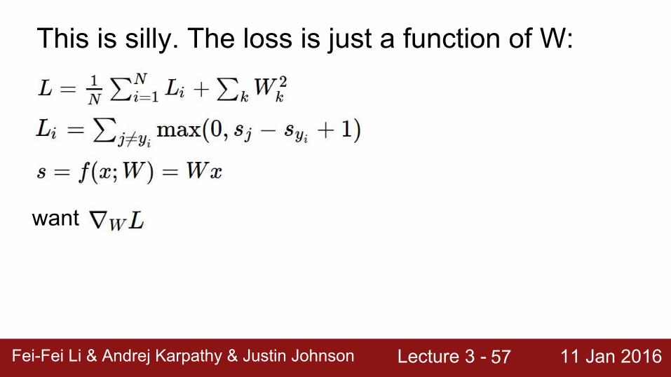
This is silly. The loss is just a function of W:
want
Lecture 3 - 11 Jan 2016Fei-Fei Li & Andrej Karpathy & Justin JohnsonFei-Fei Li & Andrej Karpathy & Justin Johnson Lecture 3 - 11 Jan 201658
This is silly. The loss is just a function of W:
want
Lecture 3 - 11 Jan 2016Fei-Fei Li & Andrej Karpathy & Justin JohnsonFei-Fei Li & Andrej Karpathy & Justin Johnson Lecture 3 - 11 Jan 201659
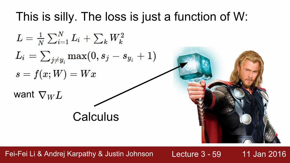
This is silly. The loss is just a function of W:
Calculus
want
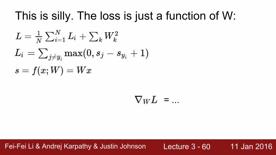
Lecture 3 - 11 Jan 2016Fei-Fei Li & Andrej Karpathy & Justin JohnsonFei-Fei Li & Andrej Karpathy & Justin Johnson Lecture 3 - 11 Jan 201660
This is silly. The loss is just a function of W:
= ...
Lecture 3 - 11 Jan 2016Fei-Fei Li & Andrej Karpathy & Justin JohnsonFei-Fei Li & Andrej Karpathy & Justin Johnson Lecture 3 - 11 Jan 201661
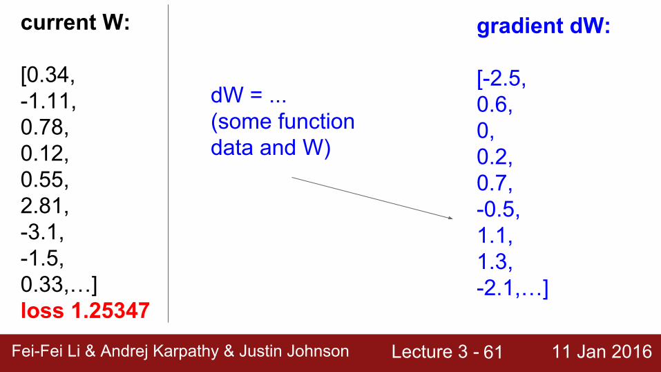
gradient dW:
[-2.5,0.6,0,0.2,0.7,-0.5,1.1,1.3,-2.1,…]
current W:
[0.34,-1.11,0.78,0.12,0.55,2.81,-3.1,-1.5,0.33,…] loss 1.25347
dW = ...(some function data and W)
Lecture 3 - 11 Jan 2016Fei-Fei Li & Andrej Karpathy & Justin JohnsonFei-Fei Li & Andrej Karpathy & Justin Johnson Lecture 3 - 11 Jan 201662
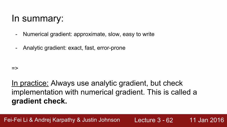
In summary:- Numerical gradient: approximate, slow, easy to write
- Analytic gradient: exact, fast, error-prone
=>
In practice: Always use analytic gradient, but check implementation with numerical gradient. This is called a gradient check.
Lecture 3 - 11 Jan 2016Fei-Fei Li & Andrej Karpathy & Justin JohnsonFei-Fei Li & Andrej Karpathy & Justin Johnson Lecture 3 - 11 Jan 201663
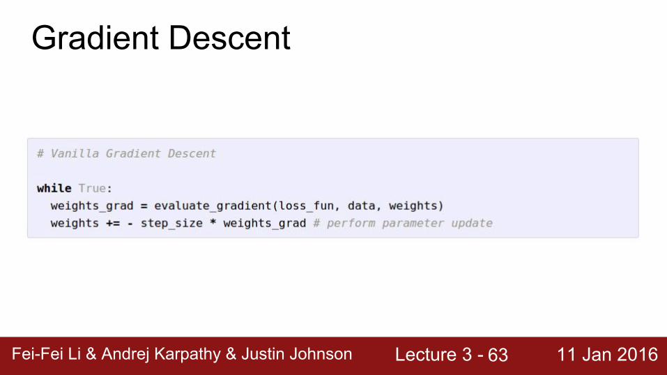
Gradient Descent

Lecture 3 - 11 Jan 2016Fei-Fei Li & Andrej Karpathy & Justin JohnsonFei-Fei Li & Andrej Karpathy & Justin Johnson Lecture 3 - 11 Jan 201664
original W
negative gradient directionW_1
W_2
Lecture 3 - 11 Jan 2016Fei-Fei Li & Andrej Karpathy & Justin JohnsonFei-Fei Li & Andrej Karpathy & Justin Johnson Lecture 3 - 11 Jan 201665
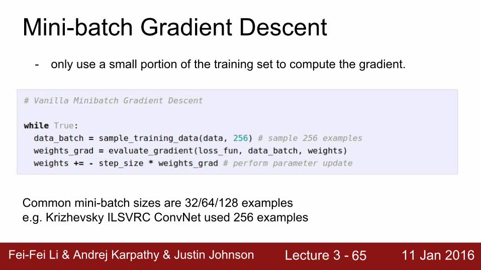
Mini-batch Gradient Descent- only use a small portion of the training set to compute the gradient.
Common mini-batch sizes are 32/64/128 examplese.g. Krizhevsky ILSVRC ConvNet used 256 examples
Lecture 3 - 11 Jan 2016Fei-Fei Li & Andrej Karpathy & Justin JohnsonFei-Fei Li & Andrej Karpathy & Justin Johnson Lecture 3 - 11 Jan 201666
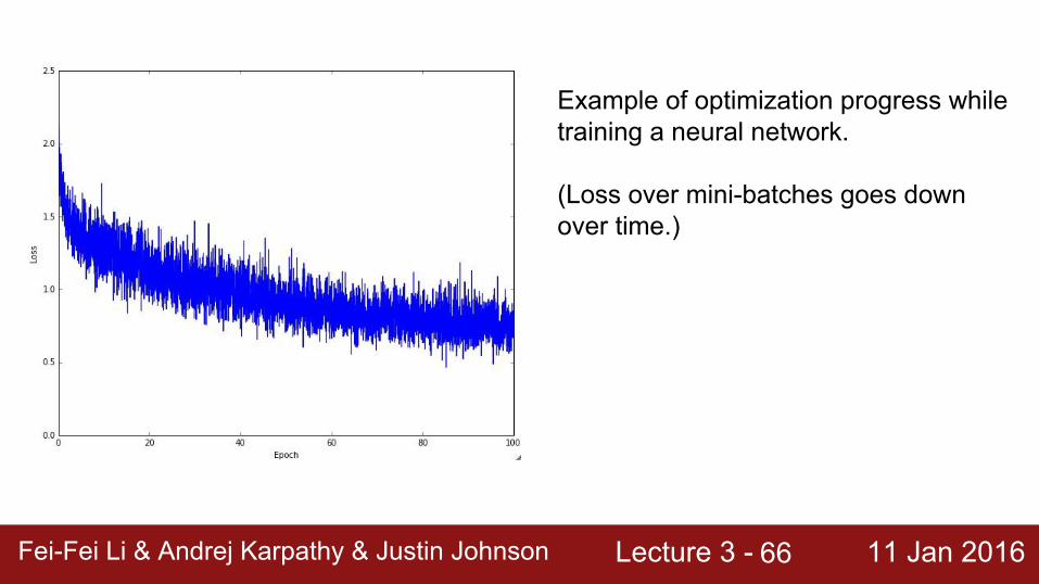
Example of optimization progress while training a neural network.
(Loss over mini-batches goes down over time.)
Lecture 3 - 11 Jan 2016Fei-Fei Li & Andrej Karpathy & Justin JohnsonFei-Fei Li & Andrej Karpathy & Justin Johnson Lecture 3 - 11 Jan 201667
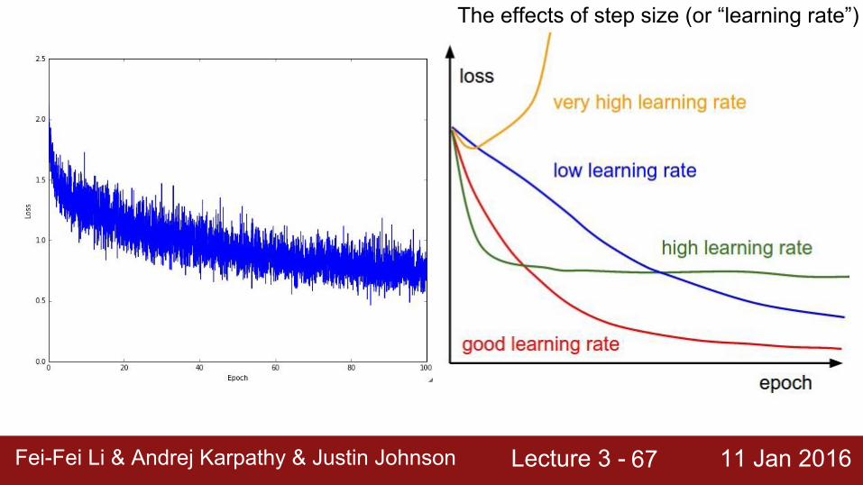
The effects of step size (or “learning rate”)
Lecture 3 - 11 Jan 2016Fei-Fei Li & Andrej Karpathy & Justin JohnsonFei-Fei Li & Andrej Karpathy & Justin Johnson Lecture 3 - 11 Jan 201668
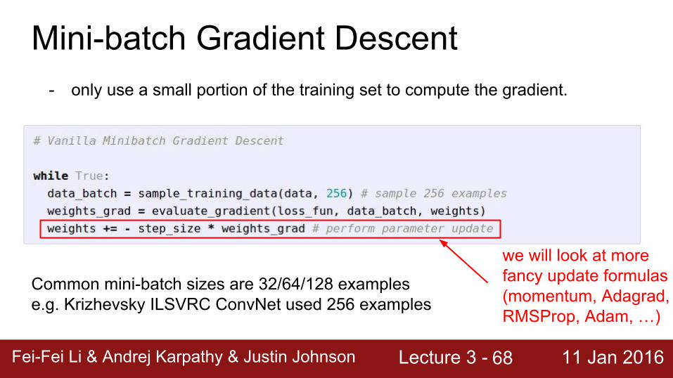
Mini-batch Gradient Descent- only use a small portion of the training set to compute the gradient.
Common mini-batch sizes are 32/64/128 examplese.g. Krizhevsky ILSVRC ConvNet used 256 examples
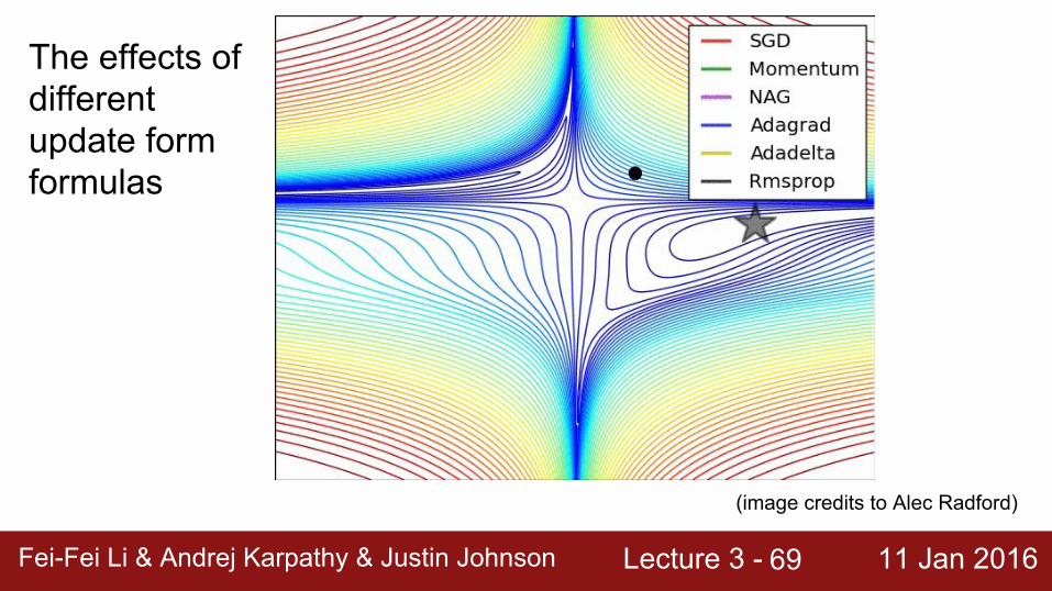
we will look at more fancy update formulas(momentum, Adagrad, RMSProp, Adam, …)
Lecture 3 - 11 Jan 2016Fei-Fei Li & Andrej Karpathy & Justin JohnsonFei-Fei Li & Andrej Karpathy & Justin Johnson Lecture 3 - 11 Jan 201669
(image credits to Alec Radford)
The effects of different update form formulas
Lecture 3 - 11 Jan 2016Fei-Fei Li & Andrej Karpathy & Justin JohnsonFei-Fei Li & Andrej Karpathy & Justin Johnson Lecture 3 - 11 Jan 201670
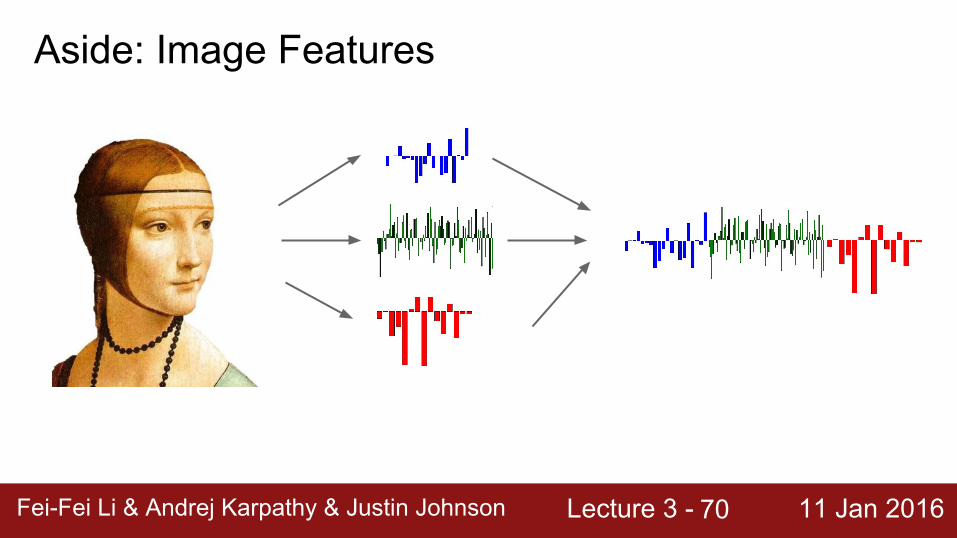
Aside: Image Features
Lecture 3 - 11 Jan 2016Fei-Fei Li & Andrej Karpathy & Justin JohnsonFei-Fei Li & Andrej Karpathy & Justin Johnson Lecture 3 - 11 Jan 201671
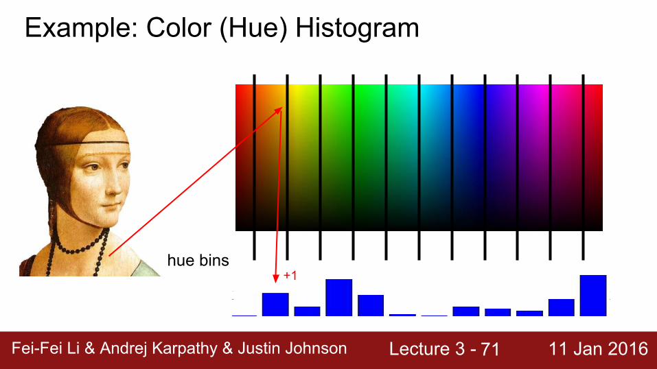
Example: Color (Hue) Histogram
hue bins+1
Lecture 3 - 11 Jan 2016Fei-Fei Li & Andrej Karpathy & Justin JohnsonFei-Fei Li & Andrej Karpathy & Justin Johnson Lecture 3 - 11 Jan 201672
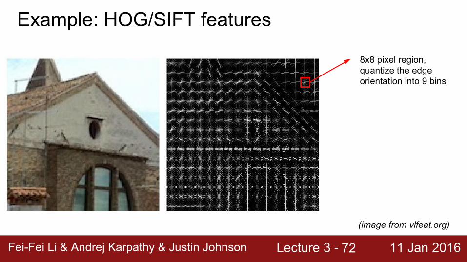
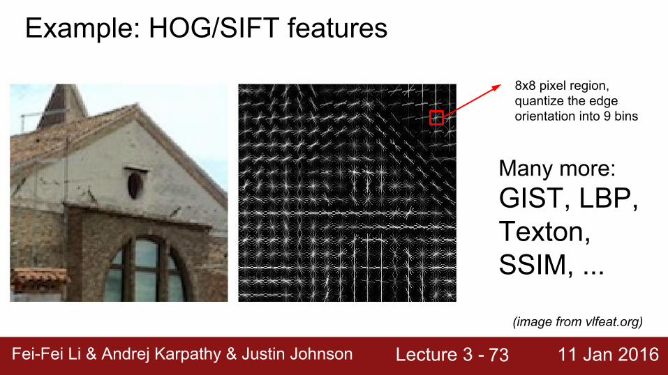
Example: HOG/SIFT features
8x8 pixel region,quantize the edge orientation into 9 bins
(image from vlfeat.org)
Lecture 3 - 11 Jan 2016Fei-Fei Li & Andrej Karpathy & Justin JohnsonFei-Fei Li & Andrej Karpathy & Justin Johnson Lecture 3 - 11 Jan 201673
Example: HOG/SIFT features
8x8 pixel region,quantize the edge orientation into 9 bins
(image from vlfeat.org)
Many more:GIST, LBP, Texton, SSIM, ...
Lecture 3 - 11 Jan 2016Fei-Fei Li & Andrej Karpathy & Justin JohnsonFei-Fei Li & Andrej Karpathy & Justin Johnson Lecture 3 - 11 Jan 201674
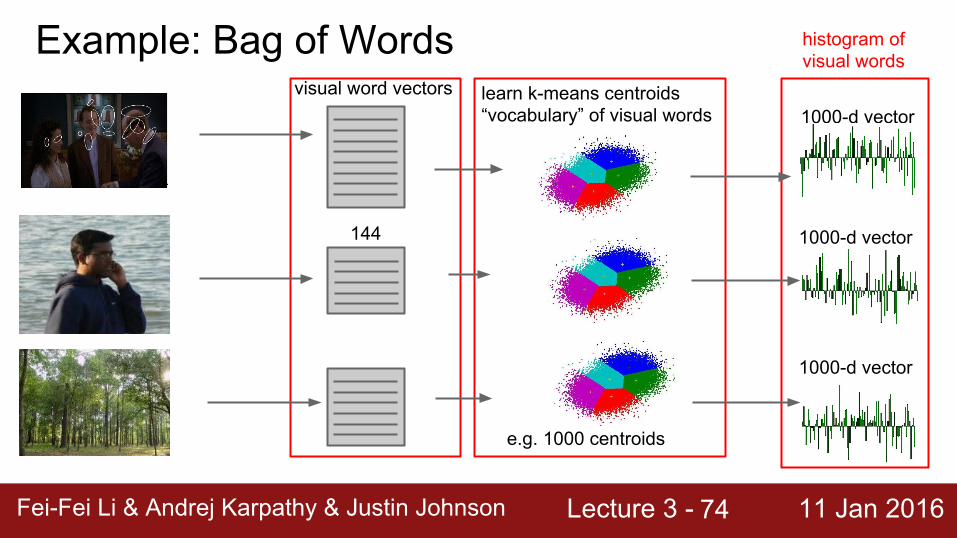
Example: Bag of Words
144
visual word vectors learn k-means centroids “vocabulary” of visual words
e.g. 1000 centroids
1000-d vector
1000-d vector
1000-d vector
histogram of visual words
Lecture 3 - 11 Jan 2016Fei-Fei Li & Andrej Karpathy & Justin JohnsonFei-Fei Li & Andrej Karpathy & Justin Johnson Lecture 3 - 11 Jan 201675
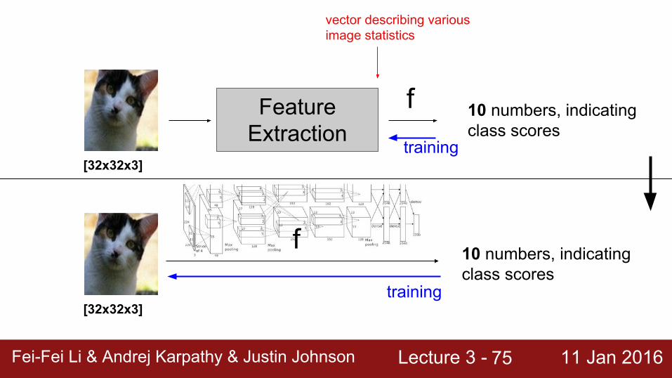
[32x32x3]
f 10 numbers, indicating class scores
Feature Extraction
vector describing various image statistics
[32x32x3]
f 10 numbers, indicating class scores
training
training
Lecture 3 - 11 Jan 2016Fei-Fei Li & Andrej Karpathy & Justin JohnsonFei-Fei Li & Andrej Karpathy & Justin Johnson Lecture 3 - 11 Jan 201676
Next class:
Becoming a backprop ninjaand
Neural Networks (part 1)


![Case Study: LeNet-5€¦ · Fei-Fei Li & Andrej Karpathy & Justin Johnson Lecture 7 -60 27 Jan 2016 Case Study: LeNet-5 [LeCun et al., 1998] Conv filters were 5x5, applied at stride](https://static.fdocuments.net/doc/165x107/60161c8688fe470c05059b01/case-study-lenet-5-fei-fei-li-andrej-karpathy-justin-johnson-lecture.jpg)
