Lect 1 Intro

Nonlinear Control

Lecture # 1

Introduction

Nonlinear Control Lecture # 1 Introduction

Nonlinear State Model

x1 = f1(t, x1, . . . , xn, u1, . . . , um)

x2 = f2(t, x1, . . . , xn, u1, . . . , um)...

...

xn = fn(t, x1, . . . , xn, u1, . . . , um)

xi denotes the derivative of xi with respect to the timevariable tu1, u2, . . ., um are input variablesx1, x2, . . ., xn the state variables


x =

x1

x2

...

...

xn

, u =

u1

u2

...

um

, f(t, x, u) =

f1(t, x, u)

f2(t, x, u)

...

...

fn(t, x, u)

x = f(t, x, u)


x = f(t, x, u)

y = h(t, x, u)

x is the state, u is the inputy is the output (q-dimensional vector)

Special Cases:Linear systems:

x = A(t)x+B(t)u

y = C(t)x+D(t)u

Unforced state equation:

x = f(t, x)

Results from x = f(t, x, u) with u = γ(t, x)


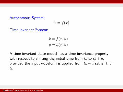
Autonomous System:x = f(x)

Time-Invariant System:

x = f(x, u)

y = h(x, u)

A time-invariant state model has a time-invariance propertywith respect to shifting the initial time from t0 to t0 + a,provided the input waveform is applied from t0 + a rather thant0


Existence and Uniqueness of Solutions

x = f(t, x)

f(t, x) is piecewise continuous in t and locally Lipschitz in xover the domain of interest

f(t, x) is piecewise continuous in t on an interval J ⊂ R if forevery bounded subinterval J0 ⊂ J , f is continuous in t for allt ∈ J0, except, possibly, at a finite number of points where fmay have finite-jump discontinuities

f(t, x) is locally Lipschitz in x at a point x0 if there is aneighborhood N(x0, r) = {x ∈ Rn | ‖x− x0‖ < r} wheref(t, x) satisfies the Lipschitz condition

‖f(t, x)− f(t, y)‖ ≤ L‖x− y‖, L > 0


A function f(t, x) is locally Lipschitz in x on a domain (openand connected set) D ⊂ Rn if it is locally Lipschitz at everypoint x0 ∈ D

When n = 1 and f depends only on x

|f(y)− f(x)|

|y − x|≤ L

On a plot of f(x) versus x, a straight line joining any twopoints of f(x) cannot have a slope whose absolute value isgreater than L

Any function f(x) that has infinite slope at some point is notlocally Lipschitz at that point


A discontinuous function is not locally Lipschitz at the pointsof discontinuity

The function f(x) = x1/3 is not locally Lipschitz at x = 0since

f ′(x) = (1/3)x−2/3 → ∞ a x → 0

On the other hand, if f ′(x) is continuous at a point x0 thenf(x) is locally Lipschitz at the same point because |f ′(x)| isbounded by a constant k in a neighborhood of x0, whichimplies that f(x) satisfies the Lipschitz condition with L = k

More generally, if for t ∈ J ⊂ R and x in a domain D ⊂ Rn,f(t, x) and its partial derivatives ∂fi/∂xj are continuous, thenf(t, x) is locally Lipschitz in x on D


Lemma 1.1

Let f(t, x) be piecewise continuous in t and locally Lipschitzin x at x0, for all t ∈ [t0, t1]. Then, there is δ > 0 such thatthe state equation x = f(t, x), with x(t0) = x0, has a uniquesolution over [t0, t0 + δ]

Without the local Lipschitz condition, we cannot ensureuniqueness of the solution. For example, x = x1/3 hasx(t) = (2t/3)3/2 and x(t) ≡ 0 as two different solutions whenthe initial state is x(0) = 0

The lemma is a local result because it guarantees existenceand uniqueness of the solution over an interval [t0, t0 + δ], butthis interval might not include a given interval [t0, t1]. Indeedthe solution may cease to exist after some time


Example 1.3

x = −x2

f(x) = −x2 is locally Lipschitz for all x

x(0) = −1 ⇒ x(t) =1

(t− 1)

x(t) → −∞ as t → 1

The solution has a finite escape time at t = 1

In general, if f(t, x) is locally Lipschitz over a domain D andthe solution of x = f(t, x) has a finite escape time te, thenthe solution x(t) must leave every compact (closed andbounded) subset of D as t → te


Global Existence and Uniqueness

A function f(t, x) is globally Lipschitz in x if

‖f(t, x)− f(t, y)‖ ≤ L‖x− y‖

for all x, y ∈ Rn with the same Lipschitz constant L

If f(t, x) and its partial derivatives ∂fi/∂xj are continuous forall x ∈ Rn, then f(t, x) is globally Lipschitz in x if and only ifthe partial derivatives ∂fi/∂xj are globally bounded, uniformlyin t

f(x) = −x2 is locally Lipschitz for all x but not globallyLipschitz because f ′(x) = −2x is not globally bounded


Lemma 1.2

Let f(t, x) be piecewise continuous in t and globally Lipschitzin x for all t ∈ [t0, t1]. Then, the state equation x = f(t, x),with x(t0) = x0, has a unique solution over [t0, t1]

The global Lipschitz condition is satisfied for linear systems ofthe form

x = A(t)x+ g(t)

but it is a restrictive condition for general nonlinear systems


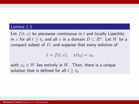
Lemma 1.3

Let f(t, x) be piecewise continuous in t and locally Lipschitzin x for all t ≥ t0 and all x in a domain D ⊂ Rn. Let W be acompact subset of D, and suppose that every solution of

x = f(t, x), x(t0) = x0

with x0 ∈ W lies entirely in W . Then, there is a uniquesolution that is defined for all t ≥ t0


Example 1.4

x = −x3 = f(x)

f(x) is locally Lipschitz on R, but not globally Lipschitzbecause f ′(x) = −3x2 is not globally bounded

If, at any instant of time, x(t) is positive, the derivative x(t)will be negative. Similarly, if x(t) is negative, the derivativex(t) will be positive

Therefore, starting from any initial condition x(0) = a, thesolution cannot leave the compact set {x ∈ R | |x| ≤ |a|}

Thus, the equation has a unique solution for all t ≥ 0


Change of Variables

Map: z = T (x), Inverse map: x = T−1(z)

Definitions

a map T (x) is invertible over its domain D if there is amap T−1(·) such that x = T−1(z) for all z ∈ T (D)

A map T (x) is a diffeomorphism if T (x) and T−1(x) arecontinuously differentiable

T (x) is a local diffeomorphism at x0 if there is aneighborhood N of x0 such that T restricted to N is adiffeomorphism on N

T (x) is a global diffeomorphism if it is a diffeomorphismon Rn and T (Rn) = Rn


Jacobian matrix

∂T

∂x=

∂T1

∂x1

∂T1

∂x2

· · · ∂T1

∂xn

......

......

......

......

∂Tn

∂x1

∂Tn

∂x2

· · · ∂Tn

∂xn

Lemma 1.4

The continuously differentiable map z = T (x) is a localdiffeomorphism at x0 if the Jacobian matrix [∂T/∂x] isnonsingular at x0. It is a global diffeomorphism if and only if[∂T/∂x] is nonsingular for all x ∈ Rn and T is proper; that is,lim‖x‖→∞ ‖T (x)‖ = ∞


Example 1.5

Negative Resistance Oscillator

x =

[

x2

−x1 − εh′(x1)x2

]

, z =

[

z2/εε[−z1 − h(z2)]

]

z = T (x) =

[

−h(x1)− x2/εx1

]

,∂T

∂x=

[

−h′(x1) −1/ε1 0

]

det(T (x) = 1/ε is positive for all x

‖T (x)‖2 = [h(x1) + x2/ε]2 + x2

1→ ∞ as ‖x‖ → ∞


Equilibrium Points

A point x = x∗ in the state space is said to be an equilibriumpoint of x = f(t, x) if

x(t0) = x∗ ⇒ x(t) ≡ x∗, ∀ t ≥ t0

For the autonomous system x = f(x), the equilibrium pointsare the real solutions of the equation

f(x) = 0

An equilibrium point could be isolated; that is, there are noother equilibrium points in its vicinity, or there could be acontinuum of equilibrium points


A linear system x = Ax can have an isolated equilibrium pointat x = 0 (if A is nonsingular) or a continuum of equilibriumpoints in the null space of A (if A is singular)

It cannot have multiple isolated equilibrium points,for if xa and xb are two equilibrium points, then by linearityany point on the line αxa + (1− α)xb connecting xa and xb

will be an equilibrium point

A nonlinear state equation can have multiple isolatedequilibrium points. For example, the state equation

x1 = x2, x2 = −a sin x1 − bx2

has equilibrium points at (x1 = nπ, x2 = 0) forn = 0,±1,±2, · · ·


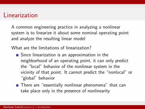
Linearization

A common engineering practice in analyzing a nonlinearsystem is to linearize it about some nominal operating pointand analyze the resulting linear model

What are the limitations of linearization?

Since linearization is an approximation in theneighborhood of an operating point, it can only predictthe “local” behavior of the nonlinear system in thevicinity of that point. It cannot predict the “nonlocal” or“global” behavior

There are “essentially nonlinear phenomena” that cantake place only in the presence of nonlinearity


Nonlinear Phenomena

Finite escape time

Multiple isolated equilibrium points

Limit cycles

Subharmonic, harmonic, or almost-periodic oscillations

Chaos

Multiple modes of behavior


Approaches to Nonlinear Control

Approximate nonlinearity

Compensate for nonlinearity

Dominate nonlinearity

Use intrinsic properties

Divide and conquer


Lect 1 Intro

Documents

Transcript of Lect 1 Intro