Lanczos Method for Eigensystems

Aiichiro Nakano Collaboratory for Advanced Computing & Simulations

Department of Computer Science Department of Physics & Astronomy

Department of Chemical Engineering & Materials Science Department of Biological Sciences University of Southern California

Email: anakano@usc.edu

B. N. Parlett!The Symmetric Eigenvalue Problem!

(Prentice-Hall, ’80) Secs. 11-13!

Rayleigh Quotient Theorem Let A be an n×n real symmetric matrix, λ1[A] ≤ … ≤ λn[A] its eigenvalues in ascending order, x ∈ Rn, & the Rayleigh quotient

then

Proof Let q(k) be the k-th orthonormalized eigenvector of A, , & orthogonal transformation matrix, , then €

ρ(x;A) =xTAxxTx

€

λ1[A] =x∈ℜnmin ρ(x;A)

λn[A] =x∈ℜnmax ρ(x;A)

⎧

⎨ ⎪

⎩ ⎪

€

Aqk = λkqk

€

Q = q1q2!qn[ ]

Let x = Qz (note QTQ = I), then

which is a weighted average of λ1, …, λn, & the minimum is when zT = (1,0,…,0) = e1 & x = Qe1 = q1.

€

QTAQ =

λ1!

λn

⎡

⎣

⎢ ⎢ ⎢

⎤

⎦

⎥ ⎥ ⎥

€

ρ(x;A) =zTQTAQzzTQTQz

=z12λ1 +!+ zn

2λnz12 +!+ zn

2

Rayleigh-Ritz Procedure Theorem Let {q1,…,qm} be an orthonormal set that spans Rm (m < n) ⊂ Rn, so that any vector x ∈ Rm is expressed as a linear combination of q1,…,qm:

or

then the best approximations for λ1[A] & λn[A] are obtained by diagonalizing

as λ1[H] & λm[H].

Proof Note

then

the minimum of which is λ1[H] (cf. proof in the previous page).

€

x = z1q1 +!+ zmqm

€

1

nx1!xn

⎡

⎣

⎢ ⎢ ⎢

⎤

⎦

⎥ ⎥ ⎥

=

m

n q1 " qm

⎡

⎣

⎢ ⎢ ⎢

⎤

⎦

⎥ ⎥ ⎥

1z1!zm

⎡

⎣

⎢ ⎢ ⎢

⎤

⎦

⎥ ⎥ ⎥

m =Qz

€

m ×mH =

m × nQT

n × nA

n ×mQ

€

ρ(x;A) =zTQTAQzzTQTQz

=zTHzzTz

=z12λ1(H )+!+ zm

2 λm (H )z12 +!+ zm

2

€

QTQ( ) ij = QkiQkjk=1

n∑ = qi • q j = δ ij 1≤ i, j ≤ m

Orthogonalization by QR Decomposition • Gram-Schmidt orthonormalization: The orthonormal set Q required for

the Rayleigh-Ritz procedure is obtained starting from an arbitrary set of m vectors, S = [s1…sm] (sj ∈ Rn) as:

€

q1 = s1 / | s1 |for i = 2 to m

ʹ′ q i = si − q j q j • si( )j=1

i−1∑

qi = ʹ′ q i / | ʹ′ q i |endfor

€

∵ si =| ʹ′ q i | qi + q j q j • si( )j=1

i−1∑

• The Gram-Schmidt amounts to QR decomposition, S = QR, where R is an m×m right-triangle matrix:

€

m

n s1 s2 s3 s4

⎡

⎣

⎢ ⎢ ⎢

⎤

⎦

⎥ ⎥ ⎥

=

m

n q1 q2 q3 q4

⎡

⎣

⎢ ⎢ ⎢

⎤

⎦

⎥ ⎥ ⎥

m| ʹ′ q 1 | q1 • s2 q1 • s3 q1 • s40 | ʹ′ q 2 | q2 • s3 q2 • s40 0 | ʹ′ q 3 | q3 • s40 0 0 | ʹ′ q 4 |

⎡

⎣

⎢ ⎢ ⎢ ⎢

⎤

⎦

⎥ ⎥ ⎥ ⎥

m

Projection!

Rayleigh-Ritz Algorithm

1. Start from S = [s1…sm] (sj ∈ Rn) & do Gram-Schmidt orthonormalization, S = QR, to obtain an orthonormal set Q = [q1…qm]

2. Form H = QTAQ

3. Diagonalize H to get λ1[H],…,λm[H]:

4. Approximations of λ1[A] & λn[A] are given by λ1[H] & λm[H] with the corresponding eigenvectors, yk = Qgk (k = 1 & m).

€

*

QTAQH

! " # gk = λk[H]gk

↓ Q ×

∴AQgky k$ ~ λk[H ]Qgk

y k$

€

Hgk = λk[H]gk (k = 1,…,m)

* QQT ≠ IN×N but spans a subspace of the N-dimensional space

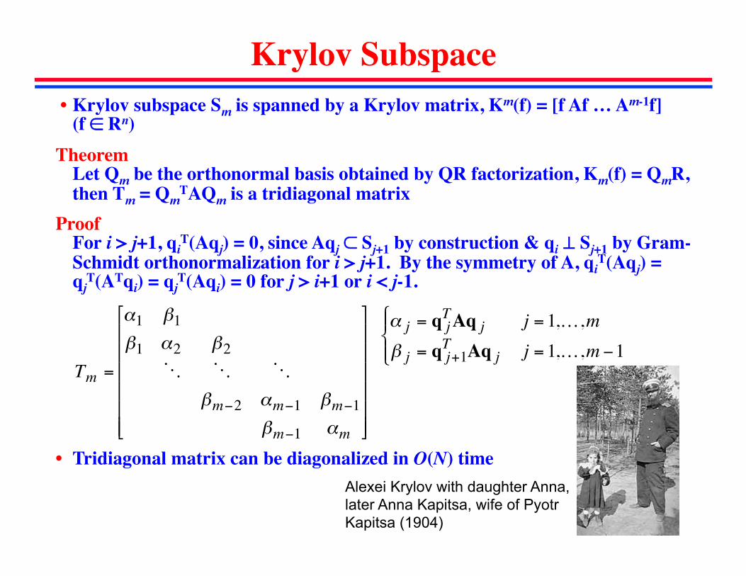
Krylov Subspace • Krylov subspace Sm is spanned by a Krylov matrix, Km(f) = [f Af … Am-1f]

(f ∈ Rn) Theorem Let Qm be the orthonormal basis obtained by QR factorization, Km(f) = QmR, then Tm = Qm

TAQm is a tridiagonal matrix Proof For i > j+1, qi

T(Aqj) = 0, since Aqj ⊂ Sj+1 by construction & qi ⊥ Sj+1 by Gram-Schmidt orthonormalization for i > j+1. By the symmetry of A, qi

T(Aqj) = qj

T(ATqi) = qjT(Aqi) = 0 for j > i+1 or i < j-1.

€

Tm =

α1 β1β1 α2 β2! ! !

βm−2 αm−1 βm−1βm−1 αm

⎡

⎣

⎢ ⎢ ⎢ ⎢ ⎢ ⎢

⎤

⎦

⎥ ⎥ ⎥ ⎥ ⎥ ⎥

€

α j = q jTAq j j = 1,…,m

β j = q j+1T Aq j j = 1,…,m −1

⎧ ⎨ ⎪

⎩ ⎪

Alexei Krylov with daughter Anna, later Anna Kapitsa, wife of Pyotr Kapitsa (1904)

• Tridiagonal matrix can be diagonalized in O(N) time

Recursion Formula

• Due to the tridiagonality, Aqi is a linear combination of qi-1, qi & qi+1:

If we define q0 = 0, the above equation is valid for i = 1 as well. Let ri ≡ βiqi+1 (ri is a component of Aqi orthogonal to qj for j ≤ i), then

• Lanczos algorithm:

€

Aqi = β i−1qi−1 +α iqi + β iqi+1 (2 ≤ i ≤ m −1)

€

ri = Aqi − β i−1qi−1 −α iqi (1≤ i ≤ m −1)

€

Given r0,β0 = r0 q0 = 0( )for i = 1,!,mqi ← ri−1 /β i−1ri ← Aqi − β i−1qi−1αi ← qi

Triri ← ri −αiqiβ i = ri only when i ≤ m −1( )

endfor

€

∵qiT (Aqi − β i−1qi−1) = qi

TAqi =α i (orthogonality)

Keep increasing m until λ1[Tm] converges

Application of Rayleigh-Ritz/Lanczos • Search for transition states (with a negative eigenvalue of the Hessian matrix, ∂2E/∂ri∂rj, by following the eigenvector with the smallest eigenvalue —Rayleigh-Ritz: Kumeda, Wales & Munro, Chem. Phys. Lett. 341, 185 (’01) ! —Lanczos: Mousseau et al., J. Mol. Graph. Model. 19, 78 (’01) !

Figure from Prof. H. B. Schlegel; http://chem.wayne.edu/schlegel!

Lanczos Algorithm for Hessian Calculation

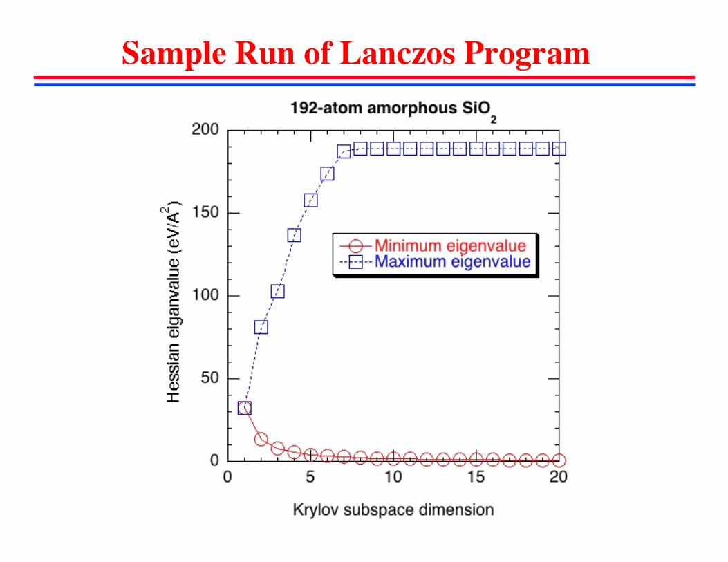
Sample Run of Lanczos Program

Electronic Energy Bands of GaAs

C. Pryor, Phys. Rev. B 57, 7190 (’98)

• 8-band k•p model

Lanczos Program in Fortran do s = 1,NWF! q(:,:,:,s) = v/bet(s-1)! call hamiltonian_op(q(:,:,:,s),hv) ! Operates Hamiltonian H on Q(S)! v = hv-bet(s-1)*q(:,:,:,s-1)! alp(s) = inner_product(q(:,:,:,s),v)! v = v-alp(s)*q(:,:,:,s)! bet(s) = sqrt(inner_product(v,v))! call tridiag(eval,s) ! Diagonalize the S by S tridiagonal matrix!end do ! Lanczos iteration S!

€

Given r0,β0 = r0 q0 = 0( )for i = 1,!,mqi ← ri−1 /β i−1ri ← Aqi − β i−1qi−1αi ← qi

Triri ← ri −αiqiβ i = ri only when i ≤ m −1( )

endfor

Band-edge Wave Functions • Band-edge states in an array of GaN quantum dots in AlN matrix

S. Sburlan, Ph.D. dissertation, USC (’13)

Valence-band top

Conduction-band states