Numerical evaluation of the Communication-AvoidingLanczos algorithm

Magnus Gustafsson∗ James Demmel† Sverker Holmgren∗

February 16, 2012

Abstract

The Lanczos algorithm is widely used for solving large sparse symmetric eigen-value problems when only a few eigenvalues from the spectrum are needed. Due tosparse matrix-vector multiplications and frequent synchronization, the algorithm iscommunication intensive leading to poor performance on parallel computers andmodern cache-based processors. The Communication-Avoiding Lanczos algorithm[Hoemmen; 2010] attempts to improve performance by taking the equivalence of ssteps of the original algorithm at a time. The scheme is equivalent to the originalalgorithm in exact arithmetic but as the value of s grows larger, numerical roundofferrors are expected to have a greater impact. In this paper, we investigate thenumerical properties of the Communication-Avoiding Lanczos (CA-Lanczos) algo-rithm and how well it works in practical computations. Apart from the algorithmitself, we have implemented techniques that are commonly used with the Lanczosalgorithm to improve its numerical performance, such as semi-orthogonal schemesand restarting. We present results that show that CA-Lanczos is often as accu-rate as the original algorithm. In many cases, if the parameters of the s-step basisare chosen appropriately, the numerical behaviour of CA-Lanczos is close to thestandard algorithm even though it is somewhat more sensitive to loosing mutualorthogonality among the basis vectors.

1 Introduction

Solving large sparse eigenvalue problems is an important and performance-critical taskin a wide range of application areas. For Hermitian problems, the symmetric Lanczosalgorithm [12] is often used, efficiently computing approximations to a few eigenvaluesof a matrix by projecting the original problem on a lower-dimensional Krylov subspace,Kk(A, v) = span

{v, Av,A2v, . . . , Ak−1v

}. In the iterative process, the Lanczos algorithm

repeatedly computes the product of the sparse matrix with a dense vector (SpMV) andinterleaves each of these SpMVs with BLAS 1 vector updates and inner products. On

∗Division of Scientific Computing, Department of Information Technology, Uppsala University, Upp-sala, Sweden (magnus.gustafsson@it.uu.se, sverker.holmgren@it.uu.se).†Department of Electrical Engineering and Computer Sciences, University of California, Berkeley,

CA, USA, (demmel@cs.berkeley.edu)

1

modern processor architectures, with deep cache hierarchies and limited memory band-width, the memory traffic incurred by the low utilization of data will be a performancebottleneck and the frequent global synchronization is a barrier for parallel scalability.

The Communication-Avoiding Lanczos algorithm (CA-Lanczos) [9] seeks to avoid thecommunication obstacles in the original Lanczos algorithm at several levels. One outeriteration of CA-Lanczos corresponds to a number of iterations (we denote it s) of theoriginal Lanczos algorithm. In one outer iteration, a block of s SpMVs are computedtogether, leaving the opportunity to reuse data in the matrix between the products. In-stead of orthogonalizing a single basis vector at a time using standard Gram-Schmidt,CA-Lanczos uses Block Gram-Schmidt (BGS) [20] and Tall Skinny QR (TSQR) [9], mini-mizing communication by sending as few messages as possible and by performing BLAS 3operations instead of the BLAS 1 operations that are used in standard Gram-Schmidtorthogonalization.

The Lanczos algorithm in its original form uses a three term recurrence relation suchthat every computed basis vector is orthogonalized against just the previous two vectors.An issue with this is that mutual orthogonality among the basis vectors is eventually lostin finite precision arithmetic, leading to slow convergence and inaccurately computedeigenvalues [19, 18, 14, 15]. The immediate fix to this problem is to extend the algorithmto include all previous basis vectors in the orthogonalization. However, as the numberof Lanczos iterations grows large, the computational effort to maintain full orthogonalityamong the basis vectors becomes increasingly demanding. To this end, several semi-orthogonal schemes have been developed that keep track of the loss of orthogonality andperform orthogonalization only when needed.

A related issue with the Lanczos algorithm is that the memory requirements grow withthe number of vectors that we need to keep. With any reorthogonalization scheme we areforced to keep all vectors and for some computations we need not only the eigenvaluesof the matrix but also the corresponding eigenvectors. For large matrices, we mightnot be able to store as many vectors as we need for the algorithm to converge. Byrestarting the method after a given number of iterations, discarding the vectors that donot contain the information we are after, we can alleviate these problems. We describeour implementation of an explicitly restarted Lanczos scheme, inspired by the methodproposed by [7], adjusted for use with CA-Lanczos.

The main objective of this paper is to evaluate the numerical performance of CA-Lanczos with explicit restart and different reorthogonalization schemes that are often usedwith the Lanczos algorithm. We use matrices from various applications (the Universityof Florida Matrix collection [4] and show that CA-Lanczos is able to compute eigenvaluesand eigenvectors to a given tolerance. We compare CA-Lanczos to the standard Lanczosalgorithm and conclude that for the most part, CA-Lanczos is almost as accurate asstandard Lanczos. We do not analyze the run time performance of CA-Lanczos in thispaper, although we address some key performance aspects that motivate the use of CA-Lanczos.

This paper is organized as follows. First, in section 2, we give an overview of theprevious work that has been done on the Lanczos algorithm in the light of communicationavoiding and s-step methods as well as restarted methods. In section 3 we briefly describethe Lanczos algorithm followed by a discussion of its well-studied numerical propertiesin Section 4. The Communication-Avoiding Lanczos algorithm (CA-Lanczos) is outlined

2

in section 5, followed by some details regarding the semi-orthogonal techniques that wehave implemented with the CA-Lanczos algorithm in section 6 and a discussion on explicitrestarting of CA-Lanczos in section 7. Finally, in section 8 we present some numericalresults, followed by concluding remarks in section 9.

2 Previous work

The Communication-Avoiding Lanczos algorithm was initially proposed by Hoemmen [9].In his thesis, he discusses communication avoiding Krylov subspace methods in generaland gives an in-depth analysis of a few chosen methods and their implementation. CA-Lanczos was derived and discussed in theory with regard to its expected numerical stabil-ity and performance. However, since eigenvalue problems were not the main focus of histhesis, CA-Lanczos was never implemented and analyzed in practical computations. Thispaper contributes to his work by assessing the numerical behaviour of the CA-Lanczosalgorithm in different application problems.

The idea of combining several iterations of Krylov subspace methods in order to im-prove performance is not new. Kim and Chronopoulos [11] introduced s-step Lanczosand s-step Arnoldi methods, as well as s-step Conjugate Gradient [3]. However, theirmethods have shown to have stability problems [22], in particular when s grows large.Furthermore, their s-step Lanczos algorithm requires s + 1 SpMVs in each outer iter-ation, as opposed to s SpMVs for an outer iteration of CA-Lanczos or s iterations ofstandard Lanczos. Thus, for large problems where the SpMV operation is the most timeconsuming part of the process, s-step Lanczos will loose much of its performance bene-fits. This is apparent in Gustafsson et al. [6], where the performance gains from avoidingsynchronization was entirely consumed by the additional SpMV in each outer iteration.

Several schemes have been proposed for explicit restart of the Lanczos algorithm (seee.g. [10], [21], [23] and [7]). The explicitly restarted schemes all have in common that therestart vector is chosen from one of the Ritz vectors in each step. In contrast, ImplicitlyRestarted Lanczos [1] iteratively applies a polynomial filter to refine the restart vector.In this work we have chosen to implement a simple explicit scheme, although ImplicitlyRestarted Lanczos is regarded to be more stable and robust.

3 The symmetric Lanczos algorithm

Given a Hermitian n × n matrix A and a starting vector v, the Lanczos method [12]successively builds a basis of the Krylov subspace

Kk(A, v) = span{v, Av,A2v, . . . , Ak−1v

}. (1)

Let Qm = [q1, q2, . . . , qm] be the orthonormal basis spanning Km(A, q1) after m steps ofthe Lanczos process, and let Tm denote the corresponding projection matrix of A ontoKm(A, q1) such that

AQm = QmTm + βm+1qm+1eTm. (2)

3

Algorithm 1 The Lanczos Algorithm

1: β1 = ‖v‖2, q0 = 0, q1 = v/β1

2: for j = 1 to convergence do3: w = Aqj − βjqj−1

4: αj = (w, qj)5: w = w − αjqj6: βj+1 = ‖w‖27: qj+1 = w/β+1

8: end for

Tm is a real, symmetric and tridiagonal m×m matrix

Tm =

α1 β2

β2 α2 β3

. . . . . . . . .

βm−1 αm−1 βm

βm αm

. (3)

Let θi denote the ith eigenvalue and si the corresponding eigenvector of Tm. Then (forall i) θi is an approximate eigenvalue (Ritz value) of A, and yi = Qmsi a correspondingapproximate eigenvector (Ritz vector) of A. Since m is usually much smaller than n,and since Tm is tridiagonal, we can compute θi and si cheaply. The Ritz vectors yi onthe other hand are much more expensive to compute since they involve the entire basismatrix Qm.

An outline of the symmetric Lanczos algorithm is presented in Algorithm 1. In ksteps, the method computes k matrix-vector products and O(k) BLAS 1 updates. Theruntime performance will normally be dominated by the SpMV on line 3. In a parallelenvironment, also the inner products on line 4 and 6 will be cumbersome since they requireglobal communication among the cores/processors. Furthermore, when the vectors aretoo large to fit in fast memory the BLAS 1 operations will generate excessive memorytraffic. On modern architectures, this will lead to poor overall performance, since off-chipmemory bandwidth is a scarce resource.

4 Orthogonality and convergence

A well-known and well-studied problem with the Lanczos algorithm is that mutual or-thogonality among the basis vectors is eventually lost in finite precision arithmetic.Paige [14, 15] showed that loss of orthogonality occurs as soon as an eigenpair is close toconvergence. If iterations are blindly continued with orthogonality lost, new Lanczos vec-tors will have components in the directions of already converged Ritz vectors and multiplecopies of previously computed Ritz values will appear [21]. Furthermore, approximationsof eigenvalues that are not true eigenvalues (spurious eigenvalues) of A may appear andmislead the results. For these reasons, lack of orthogonality among the basis vectors willslow down convergence and impair the accuracy.

Most practical computations using the Lanczos method require that the scheme isextended with some form of reorthogonalization of the basis vectors in addition to the

4

local orthogonalization of the three term recurrence. Which strategy is the most efficientwill depend on the nature of the problem at hand and the requirements on the computedeigenvalues and eigenvectors. The crudest approach, in which every new basis vector isorthogonalized against all previous basis vectors, is referred to as full orthogonalization.This is the computationally most expensive option but it is also the most accurate sinceit maintains full orthogonality among all the basis vectors at all times. We considerfull orthogonalization as the baseline result for accuracy but it is worth noting that fullorthogonalization is often not viable in practice since it incurs a significant performanceoverhead when the number of Lanczos vectors grows large. Furthermore, orthogonalityamong the basis vectors to machine precision is not required for the Lanczos algorithmto be accurate and stable. It was shown by Paige [14, 15], Simon [19, 18] and Grcar [5]that it is sufficient for the orthogonalization error to be kept below

√εM , where εM is the

machine roundoff error. This is further described in Section 6, where we discuss varioussemi-orthogonal techniques that are commonly used with the Lanczos algorithm.

5 The communication-avoiding symmetric

Lanczos algorithm (CA-Lanczos)

The Krylov subspace sequence of vectors, {v, Av,A2v, . . . , Asv}, gives good motivation fora scheme that breaks the data dependencies between iterations in the Lanczos algorithmand computes s SpMVs using a single kernel, potentially saving a factor of s reads of Afrom memory. The resulting method, referred to as the Communication-Avoiding Lanczosalgorithm (CA-Lanczos), was derived in detail in [9] so we will only give a summary of ithere.

5.1 Notation

We borrow the block-vector notation from [9], summarized as follows.

• Vectors and group of vectors:

– vk denotes a single vector

– Vk denotes a group of s vectors in outer iteration k;e.g. Vk = [vsk+1, vsk+2, . . . , vsk+s]

– Vk denotes a collection of groups of vectors at outer iteration k;e.g. Vk = [V1, V2, . . . , Vk]

• Groups of basis vectors:

– Consider the matrix of basis vectors

V k = [vsk+1, vsk+2, . . . , vsk+s+1].

– We use the following short hand notation for groups of basis vectors, whereunderline implies an additional vector at the end and the accent means a shift

5

one step to the right.

Vk = [vsk+1, vsk+2, . . . , vsk+s],

V k = [Vk, vsk+s+1],

Vk = [vsk+2, . . . , vsk+s],

V k = [Vk, vsk+s+1].

5.2 Computational kernels

In this section we describe the computational kernels on which the the CA-Lanczos algo-rithm relies.

5.2.1 Matrix powers kernel

The matrix powers kernel takes a sparse n× n matrix A, a dense vector of length n anda set of polynomials p0(z), p1(z), . . . , ps(z), where pj(z) is of degree j, and computes

V = [v1, v2, . . . , vs+1] = [p0(A)v, p1(A)v, . . . , ps(A)v], (4)

where the vectors in V form a basis for the Krylov subspace

Ks+1(A, v) = span{v,Av,A2v, . . . , Asv

}. (5)

Ideally, the matrix powers kernel requires just one message to be sent in parallel tocompute all the vectors in (4). Furthermore, the matrix A and the vector v only need tobe read once. This effectively leads to a factor of Θ(s) reduction in memory traffic anda factor of Θ(s) fewer messages in parallel.

By choosing the polynomial coefficients in (4), we can affect the numerical propertiesof the matrix powers kernel. The change of basis matrix B, which is s + 1 by s, shouldsatisfy

AV = V B. (6)

For a detailed derivation and analysis of the different bases for the matrix powerskernel and the Leja orderings we refer to Hoemmen [9] and Carson et al. [2].

Monomial basis The simplest basis for the matrix powers kernel, the monomial basis,directly corresponds to the Krylov vector sequence with pk(A) = Ak. We have

V =[v,Av,A2v, . . . , Asv

]. (7)

The corresponding change of basis matrix is

B = (e2, e3, . . . , es+1) . (8)

The monomial basis corresponds to taking s steps with the power method, which isinherently unstable since the basis vectors successively become more and more linearlydependent.

6

Newton basis The Newton basis applies polynomial shifts θi to the matrix powerskernel as follows

V =

[v, (A− θ1I)v, (A− θ2I)(A− θ1I)v, . . . ,

s∏i=1

(A− θiI)v

], (9)

with the change of basis matrix

B =

θ1

1 θ2

. . . . . .

1 θs

1

. (10)

The shifts can be obtained from a set of approximate eigenvalues of A, ordered accord-ing to the Leja ordering for complex arithmetic, or the modified Leja ordering for realarithmetic. The approximate eigenvalues can be generated by taking a few steps withthe original Lanczos algorithm if they are not available by other means.

5.2.2 Block Gram-Schmidt and Tall-Skinny QR

The original Lanczos algorithm uses Gram-Schmidt to orthogonalize the basis vectorsone at a time. CA-Lanczos on the other hand, treats a block of s vectors simultaneously,and uses block Gram-Schmidt (BGS) to orthogonalize those s vectors with respect tothe orthogonal basis of already computed Lanczos vectors [9, 20]. With a block size of svectors, BGS saves a factor of Θ(s) in the number of messages sent in parallel and a factorof Θ(s) in the number of words transferred between slow and fast memory compared tostandard Gram-Schmidt [9]. Throughout this work we have used Classical Gram-Schmidtin our implementation of BGS, although Modified Gram-Schmidt is considered to be moreaccurate. The motivation for this is that Classical Gram-Schmidt has more appealingparallel characteristics than Modified Gram-Schmidt [9, 20, 7]. However, both methodscan be used interchangeably in the BGS kernel [9].

Using BGS to orthogonalize a block of vectors Vk against an orthogonal basis Qk−1

makes the vectors in Vk orthogonal to those in Qk−1, but the vectors in Vk are not madeorthogonal to each other. We use Tall-skinny QR (TSQR) [9, 8] in order to obtain mutualorthogonality among the vectors in Vk, such that Vk = QkRkk, where Vk and Qk are n×mand Rkk is m ×m. TSQR has shown to be communication optimal for matrices wheren � m (i.e. many more rows than columns) [9, 13]. For an extensive discussion andanalysis of TSQR, c.f. [9, 8].

If BGS and TSQR are used as described above to orthogonalize Vk against Qk−1, it isnot guaranteed that the generated basis vectors in Qk are fully orthogonal to Qk−1 [9, 20].Those vectors for which the norm drops by more than a factor 2 in the orthogonalizationstep have to be reorthogonalized by doing a second pass of BGS [20]. If the vectors arestill not orthogonal, we declare an orthogonalization fault (c.f. [20] for details on how torecover from such a situation).

7

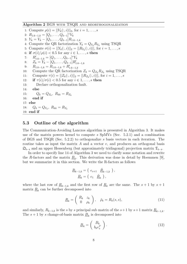
Algorithm 2 BGS with TSQR and reorthogonalization

1: Compute ρ(i) = ||Vk(:, i)||2, for i = 1, . . . , s2: R1:k−1,k = [Q1, . . . , Qk−1]

∗Vk

3: Yk = Vk − [Q1, . . . , Qk−1]R1:k−1,k

4: Compute the QR factorization Yk = QYkRYk

using TSQR5: Compute σ(i) = ||Yk(:, i)||2 = ||RYk

(:, i)||, for i = 1, . . . , s6: if σ(i)/ρ(i) < 0.5 for any i ∈ 1, . . . , s then7: R′1:k−1,k = [Q1, . . . , Qk−1]

∗Yk

8: Zk = Yk − [Q1, . . . , Qk−1]R′1:k−1,k

9: R1:k−1,k = R1:k−1,k +R′1:k−1,k

10: Compute the QR factorization Zk = QZkRZk

using TSQR11: Compute τ(i) = ||Zk(:, i)||2 = ||RZk

(:, i)||, for i = 1, . . . , s12: if τ(i)/σ(i) < 0.5 for any i ∈ 1, . . . , s then13: Declare orthogonalization fault.14: else15: Qk = QZk

, Rkk = RZk

16: end if17: else18: Qk = QYk

, Rkk = RYk

19: end if

5.3 Outline of the algorithm

The Communication-Avoiding Lanczos algorithm is presented in Algorithm 3. It makesuse of the matrix powers kernel to compute s SpMVs (Sec. 5.2.1) and a combinationof BGS and TSQR (Sec. 5.2.2) to orthogonalize s basis vectors in each iteration. Theroutine takes as input the matrix A and a vector v, and produces an orthogonal basisQt−1 and an upper Hessenberg (but approximately tridiagonal) projection matrix Tt−1.

In order to specify line 14 of Algorithm 3 we need to clarify some notation and rewritethe R-factors and the matrix Bk. This derivation was done in detail by Hoemmen [9],but we summarize it in this section. We write the R-factors as follows

Rk−1,k =(es+1 Rk−1,k

),

Rk =(e1 Rk

),

where the last row of Rk−1,k and the first row of Rk are the same. The s + 1 by s + 1matrix Rk can be further decomposed into

Rk =

(Rk zk

0 ρk

), ρk = Rk(s, s), (11)

and similarly, Rk−1,k is the s by s principal sub matrix of the s+1 by s+1 matrix Rk−1,k.The s+ 1 by s change-of-basis matrix Bk is decomposed into

Bk =

(Bk

bkeTs

). (12)

8

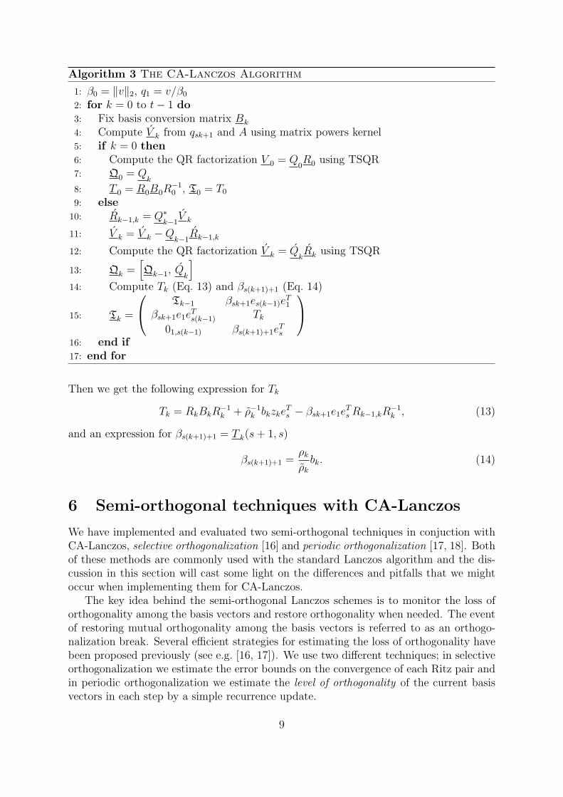
Algorithm 3 The CA-Lanczos Algorithm

1: β0 = ‖v‖2, q1 = v/β0

2: for k = 0 to t− 1 do3: Fix basis conversion matrix Bk

4: Compute V k from qsk+1 and A using matrix powers kernel5: if k = 0 then6: Compute the QR factorization V 0 = Q

0R0 using TSQR

7: Q0 = Qk

8: T 0 = R0B0R−10 , T0 = T0

9: else10: Rk−1,k = Q∗

k−1V k

11: V k = V k −Qk−1Rk−1,k

12: Compute the QR factorization V k = QkRk using TSQR

13: Qk =[Qk−1, Qk

]14: Compute Tk (Eq. 13) and βs(k+1)+1 (Eq. 14)

15: Tk =

Tk−1 βsk+1es(k−1)eT1

βsk+1e1eTs(k−1) Tk

01,s(k−1) βs(k+1)+1eTs

16: end if17: end for

Then we get the following expression for Tk

Tk = RkBkR−1k + ρ−1

k bkzkeTs − βsk+1e1e

Ts Rk−1,kR

−1k , (13)

and an expression for βs(k+1)+1 = T k(s+ 1, s)

βs(k+1)+1 =ρk

ρk

bk. (14)

6 Semi-orthogonal techniques with CA-Lanczos

We have implemented and evaluated two semi-orthogonal techniques in conjuction withCA-Lanczos, selective orthogonalization [16] and periodic orthogonalization [17, 18]. Bothof these methods are commonly used with the standard Lanczos algorithm and the dis-cussion in this section will cast some light on the differences and pitfalls that we mightoccur when implementing them for CA-Lanczos.

The key idea behind the semi-orthogonal Lanczos schemes is to monitor the loss oforthogonality among the basis vectors and restore orthogonality when needed. The eventof restoring mutual orthogonality among the basis vectors is referred to as an orthogo-nalization break. Several efficient strategies for estimating the loss of orthogonality havebeen proposed previously (see e.g. [16, 17]). We use two different techniques; in selectiveorthogonalization we estimate the error bounds on the convergence of each Ritz pair andin periodic orthogonalization we estimate the level of orthogonality of the current basisvectors in each step by a simple recurrence update.

9

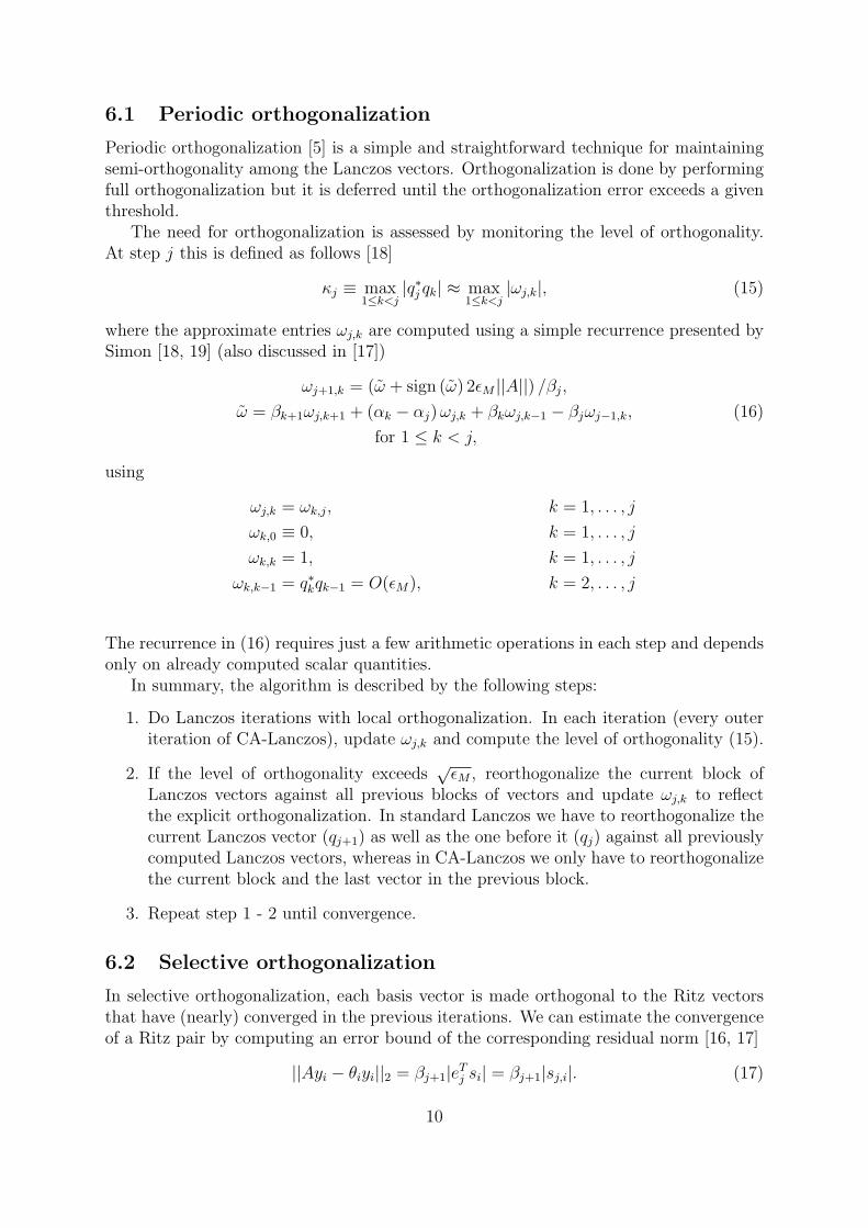
6.1 Periodic orthogonalization

Periodic orthogonalization [5] is a simple and straightforward technique for maintainingsemi-orthogonality among the Lanczos vectors. Orthogonalization is done by performingfull orthogonalization but it is deferred until the orthogonalization error exceeds a giventhreshold.

The need for orthogonalization is assessed by monitoring the level of orthogonality.At step j this is defined as follows [18]

κj ≡ max1≤k<j

|q∗j qk| ≈ max1≤k<j

|ωj,k|, (15)

where the approximate entries ωj,k are computed using a simple recurrence presented bySimon [18, 19] (also discussed in [17])

ωj+1,k = (ω + sign (ω) 2εM ||A||) /βj,

ω = βk+1ωj,k+1 + (αk − αj)ωj,k + βkωj,k−1 − βjωj−1,k, (16)

for 1 ≤ k < j,

using

ωj,k = ωk,j, k = 1, . . . , j

ωk,0 ≡ 0, k = 1, . . . , j

ωk,k = 1, k = 1, . . . , j

ωk,k−1 = q∗kqk−1 = O(εM), k = 2, . . . , j

The recurrence in (16) requires just a few arithmetic operations in each step and dependsonly on already computed scalar quantities.

In summary, the algorithm is described by the following steps:

1. Do Lanczos iterations with local orthogonalization. In each iteration (every outeriteration of CA-Lanczos), update ωj,k and compute the level of orthogonality (15).

2. If the level of orthogonality exceeds√εM , reorthogonalize the current block of

Lanczos vectors against all previous blocks of vectors and update ωj,k to reflectthe explicit orthogonalization. In standard Lanczos we have to reorthogonalize thecurrent Lanczos vector (qj+1) as well as the one before it (qj) against all previouslycomputed Lanczos vectors, whereas in CA-Lanczos we only have to reorthogonalizethe current block and the last vector in the previous block.

3. Repeat step 1 - 2 until convergence.

6.2 Selective orthogonalization

In selective orthogonalization, each basis vector is made orthogonal to the Ritz vectorsthat have (nearly) converged in the previous iterations. We can estimate the convergenceof a Ritz pair by computing an error bound of the corresponding residual norm [16, 17]

||Ayi − θiyi||2 = βj+1|eTj si| = βj+1|sj,i|. (17)

10

This is inexpensive to compute since for each i it only involves the scalars βj+1 and sj,i,where sj,i is the bottom element of eigenvector i of the projection matrix (Tj in Lanczos,Tk in CA-Lanczos). In the standard Lanczos algorithm, Tj is tridiagonal by definitionso we can compute its eigenvectors efficiently. In CA-Lanczos on the other hand, Tk isonly approximately tridiagonal and stored as a full matrix. This makes the eigenvaluedecomposition of Tk slightly more expensive to compute than that of Tj. The totalcost might be lower though, since we only need to compute the eigenvectors every outeriteration of CA-Lanczos. Furthermore, we might do as well with the eigendecompositionof just the tridiagonal part of Tk for computing (17). This performance aspect has notbeen studied in this work, since performance is not the main subject of this paper.

In summary, the Lanczos algorithm with selective orthogonalization proceeds as fol-lows [16]:

1. Do Lanczos iterations with local orthogonalization. In each iteration (every outeriteration of CA-Lanczos), estimate the convergence of each Ritz pair.

2. If there are newly converged Ritz pairs, compute all converged Ritz vectors (i.e.the previously computed Ritz vectors need to be recomputed).

3. In the subsequent Lanczos iterations, every new basis vector is orthogonalized lo-cally and made orthogonal to all converged Ritz vectors.

4. Repeat steps 2-3 until convergence.

6.3 Comparison of the cost of an orthogonalization break

Upon an orthogonalization break with periodic orthogonalization, orthogonality is re-stored by reorthogonalizing the current block of vectors against all the previous vectorsin the Krylov basis. This operation becomes increasingly expensive as the number ofLanczos vectors grows but no additional arithmetic operations are required on a break.On the other hand, when an orthogonalization break occurs with selective orthogonaliza-tion, a significant amount of extra arithmetic is introduced by the explicit regenerationof the set of converged Ritz vectors. As the number of converged Ritz vectors increases,the cost of computing the Ritz vectors increase, as does the orthogonalization against theconverged set that needs to be done in each step of the Lanczos algorithm.

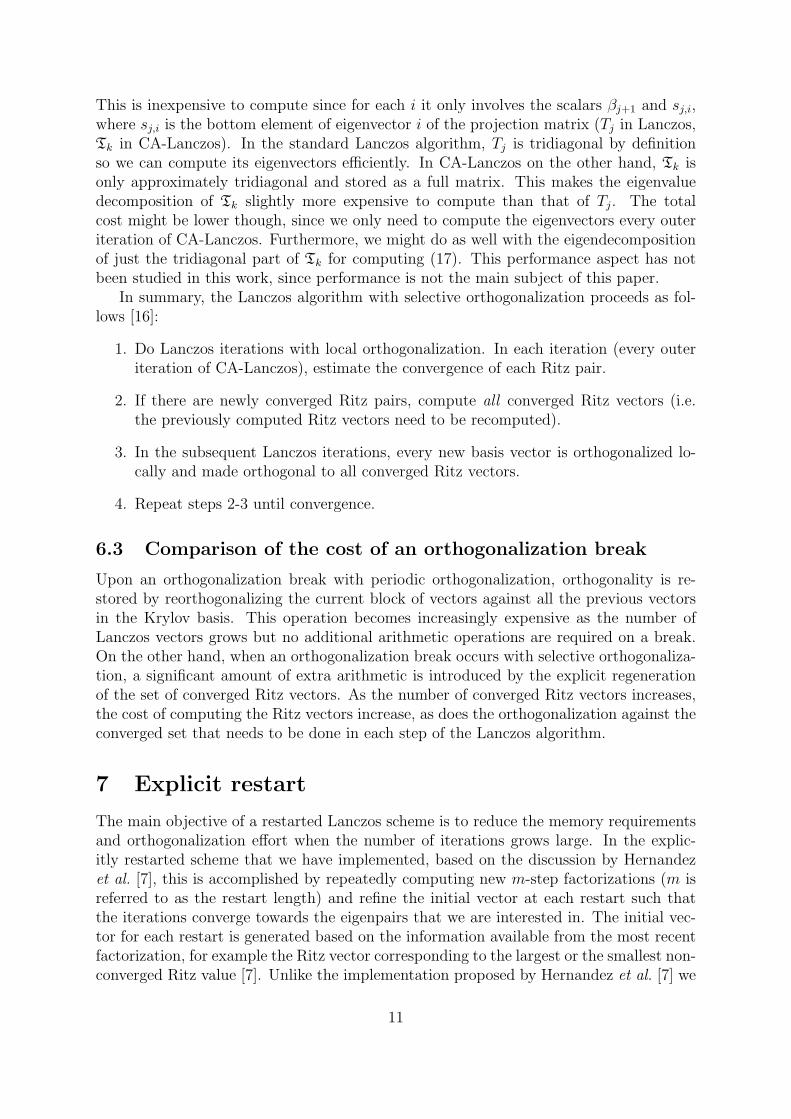
7 Explicit restart

The main objective of a restarted Lanczos scheme is to reduce the memory requirementsand orthogonalization effort when the number of iterations grows large. In the explic-itly restarted scheme that we have implemented, based on the discussion by Hernandezet al. [7], this is accomplished by repeatedly computing new m-step factorizations (m isreferred to as the restart length) and refine the initial vector at each restart such thatthe iterations converge towards the eigenpairs that we are interested in. The initial vec-tor for each restart is generated based on the information available from the most recentfactorization, for example the Ritz vector corresponding to the largest or the smallest non-converged Ritz value [7]. Unlike the implementation proposed by Hernandez et al. [7] we

11

Algorithm 4 Explictly Restarted CA-Lanczos

1: Let m: restart length (multiple of s for CA-Lanczos)2: k = 03: while k < number of wanted eigenvalues do4: Take m Lanczos steps (Algorithm 1 or 3) with initial vector vk+1, AVm = VmTm

5: Compute eigenpairs of Tm, Tmyi = yiθi

6: Compute residual norm estimates, τi = βm+1 |e∗myi|7: for each converged eigenpair θi, yi do8: k = k + 19: Ek = θi

10: Vk = Vmyi

11: end for12: end while

keep the restart length fixed between restarts. Otherwise, in particular for large valuesof s, there may be significant variances in the number of iterations for the inner Lanczoskernel to do which would lead to slow or unpredictible convergence properties. In ourimplementation, we need to keep a total of m+nw Lanczos vectors in memory, where nw

is the number of wanted eigenvalues specified by the user.At each restart, the approximate residual norm of every Ritz pair is computed and

those Ritz pairs for which the residual norm fulfills the tolerance are locked. In order tolock a Ritz pair, we compute the Ritz vector and save it together with its correspondingRitz value. After k Ritz pairs have been locked, we denote the full vector basis

Vk+m = [ Vk | Vm ] =[V

(l)1:k | V

(a)k+1:k+m

](18)

where the superscript (l) denotes the set of locked vectors and (a) the set of active vectorsthat have not yet converged [7]. In all subsequent restarts, the computed Lanczos vectorsare kept orthogonal against the k converged ones (the converged vectors are deflated)and no further modifications are done to the converged Ritz pairs. In every iteration ofthe restart loop, the inner Lanczos routine operates on the m− k active Ritz pairs

The choice of restart length is highly problem dependent and has a significant impacton the overall performance. If the restart length is too short, iterations will converge veryslowly (if at all) since we loose a little bit of information every time we throw vectors away.If it is too large, orthogonality may be lost or lead to severe performance degradation ifthe number of vectors to orthogonalize against is very large.

8 Numerical experiments

In this section, we assess the numerical behaviour of the CA-Lanczos algorithm withrespect to convergence, orthogonality and accuracy of the computed eigenvalues. Wecompare the efficiency of the orthogonalization techniques that were discussed in Section 6and evaluate the accuracy and stability of CA-Lanczos with explicit restart, described inSection 7.

Throughout the numerical experiments we have tracked the convergence of the Ritzpairs and the orthogonalization error. The convergence of a Ritz pair is described by its

12

residual norm, which (for Ritz pair i) is computed as ||Ayi − θiyi||2/||θiyi||2, where θi isthe ith eigenvalue and yi the corresponding Ritz vector of A. The orthogonalization erroris defined as the maximum of ||I −Q∗mQm||F . For the semi-orthogonal schemes we havealso tracked the number of times iterations are interrupted in order to reorthogonalizethe basis vectors, an event referred to as an orthogonalization break.

We have selected a few matrices with different properties for evaluation of our im-plementation, ranging from simple diagonal matrices to complex matrices from variousapplications. All matrices are symmetric positive definite and real but they differ instructure, condition number and eigenvalue distribution. For each matrix we have per-formed two experiments. In the first experiment we analyze the convergence behaviourof the CA-Lanczos algorithm, for different lengths of the s-step basis and for differentorthogonalization strategies. We let the iterations go way beyond the point where thelargest Ritz pair has converged, in order to see how well orthogonality is preserved. Inthe second experiment we evaluate the numerical performance of the explicitly restartedscheme. We iterate until the 10 largest eigenvalues have converged to a tolerance on therelative residual norm of 10−8, using a restart length of 60 iterations. In all experimentswe have used a vector of all ones as a starting vector.

8.1 Diagonal matrices

As a basic test case for verification and analysis, we use diagonal matrices with equallyspaced eigenvalues. By choosing the range over which we distribute the eigenvalues, wecan vary the condition numbers of the matrices. These simple matrices are also a goodstarting point since we can easily verify the correctness of the computed eigenvalues.

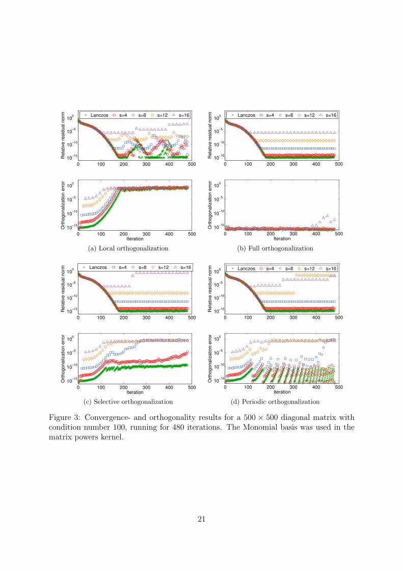
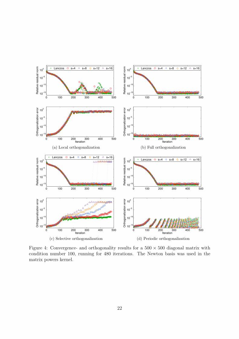
Convergence and orthogonality Convergence- and orthogonality results for a diago-nal matrix of size 500×500 with condition number 100 are shown in Figures 3 and 4 for themonomial basis and the Newton basis respectively. The relative errors in the computedeigenvalues are given in Table 1 and in Table 2 we list the number of orthogonalizationbreaks using selective and periodic orthogonalization for each basis. Comparing the re-sults for the two bases, it is immediately apparent that the Newton basis manages muchbetter than the monomial basis does in this case. For the monomial basis, the residualnorm and the orthogonalization error grows exponentially with s. For large values of s,the error in the largest eigenvalue grows out of control except with full orthogonaliza-tion where we still get an error of ∼ 10−7. With the Newton basis on the other hand,orthogonality is well preserved with full orthogonalization as well as periodic orthogo-nalization. With selective orthogonalization, orthogonality among the Lanczos vectorsslowly diminishes and for s ≥ 8 the final error in the largest eigenvalue is unacceptable.Local orthogonalization quickly loses orthogonality, but still maintains the accuracy ofthe converged eigenvalues.

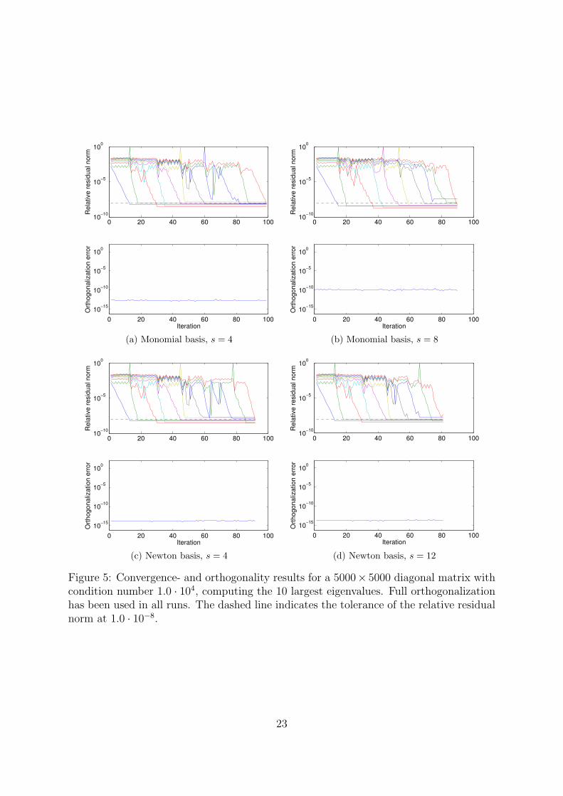
Restart In Figure 5 we present convergence- and orthogonality results for the explic-itly restarted scheme, computing the 10 largest eigenvalues of a diagonal matrix withcondition number 1.0 · 104. The dimension of this matrix is 5000. As a reference, we alsoplot the specified tolerance at 1.0 · 10−8. Clearly, the monomial basis suffers from badscaling since the orthogonalization error is significantly larger than for the corresponding

13

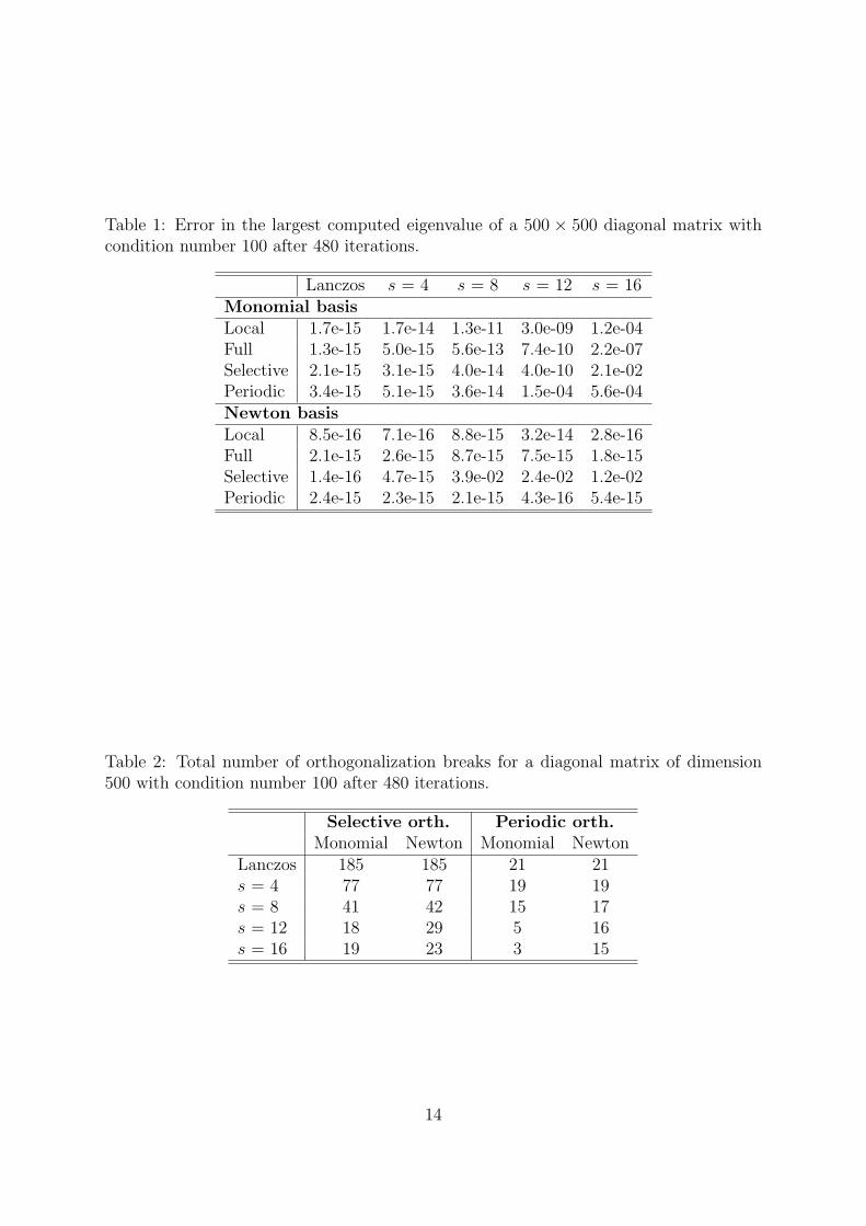
Table 1: Error in the largest computed eigenvalue of a 500 × 500 diagonal matrix withcondition number 100 after 480 iterations.

Lanczos s = 4 s = 8 s = 12 s = 16Monomial basisLocal 1.7e-15 1.7e-14 1.3e-11 3.0e-09 1.2e-04Full 1.3e-15 5.0e-15 5.6e-13 7.4e-10 2.2e-07Selective 2.1e-15 3.1e-15 4.0e-14 4.0e-10 2.1e-02Periodic 3.4e-15 5.1e-15 3.6e-14 1.5e-04 5.6e-04Newton basisLocal 8.5e-16 7.1e-16 8.8e-15 3.2e-14 2.8e-16Full 2.1e-15 2.6e-15 8.7e-15 7.5e-15 1.8e-15Selective 1.4e-16 4.7e-15 3.9e-02 2.4e-02 1.2e-02Periodic 2.4e-15 2.3e-15 2.1e-15 4.3e-16 5.4e-15

Table 2: Total number of orthogonalization breaks for a diagonal matrix of dimension500 with condition number 100 after 480 iterations.

Selective orth. Periodic orth.Monomial Newton Monomial Newton

Lanczos 185 185 21 21s = 4 77 77 19 19s = 8 41 42 15 17s = 12 18 29 5 16s = 16 19 23 3 15

14

0 50 100 150 200 250 300 35010

0

101

102

103

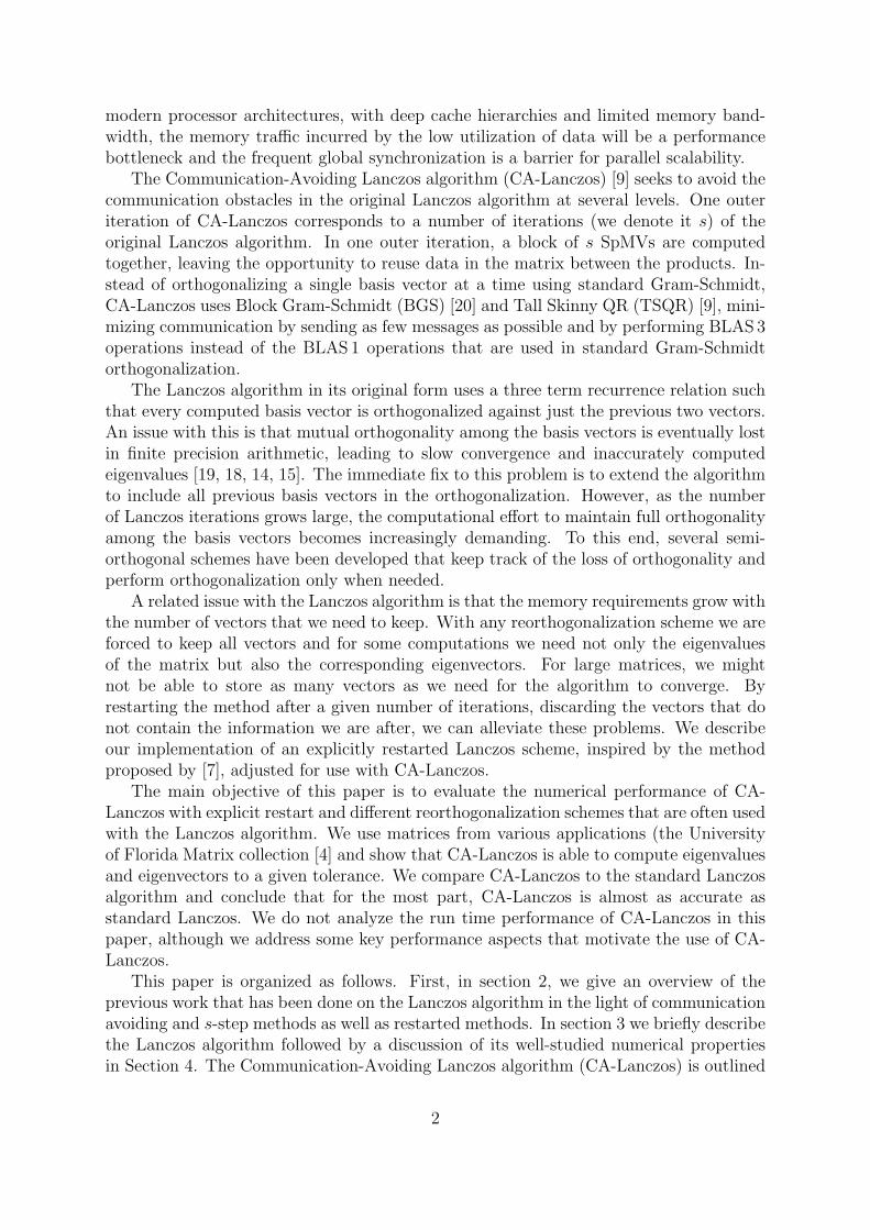
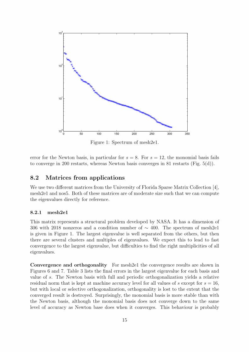
Figure 1: Spectrum of mesh2e1.

error for the Newton basis, in particular for s = 8. For s = 12, the monomial basis failsto converge in 200 restarts, whereas Newton basis converges in 81 restarts (Fig. 5(d)).

8.2 Matrices from applications

We use two different matrices from the University of Florida Sparse Matrix Collection [4],mesh2e1 and nos5. Both of these matrices are of moderate size such that we can computethe eigenvalues directly for reference.

8.2.1 mesh2e1

This matrix represents a structural problem developed by NASA. It has a dimension of306 with 2018 nonzeros and a condition number of ∼ 400. The spectrum of mesh2e1is given in Figure 1. The largest eigenvalue is well separated from the others, but thenthere are several clusters and multiples of eigenvalues. We expect this to lead to fastconvergence to the largest eigenvalue, but difficulties to find the right multiplicities of alleigenvalues.

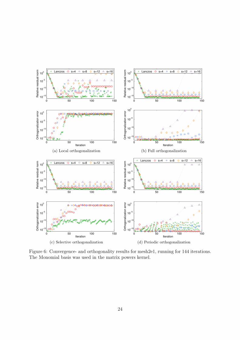
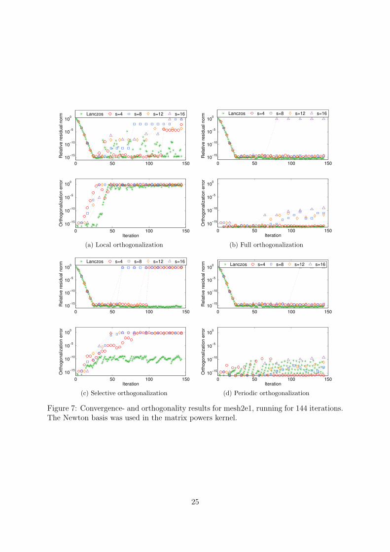
Convergence and orthogonality For mesh2e1 the convergence results are shown inFigures 6 and 7. Table 3 lists the final errors in the largest eigenvalue for each basis andvalue of s. The Newton basis with full and periodic orthogonalization yields a relativeresidual norm that is kept at machine accuracy level for all values of s except for s = 16,but with local or selective orthogonalization, orthogonality is lost to the extent that theconverged result is destroyed. Surprisingly, the monomial basis is more stable than withthe Newton basis, although the monomial basis does not converge down to the samelevel of accuracy as Newton base does when it converges. This behaviour is probably

15

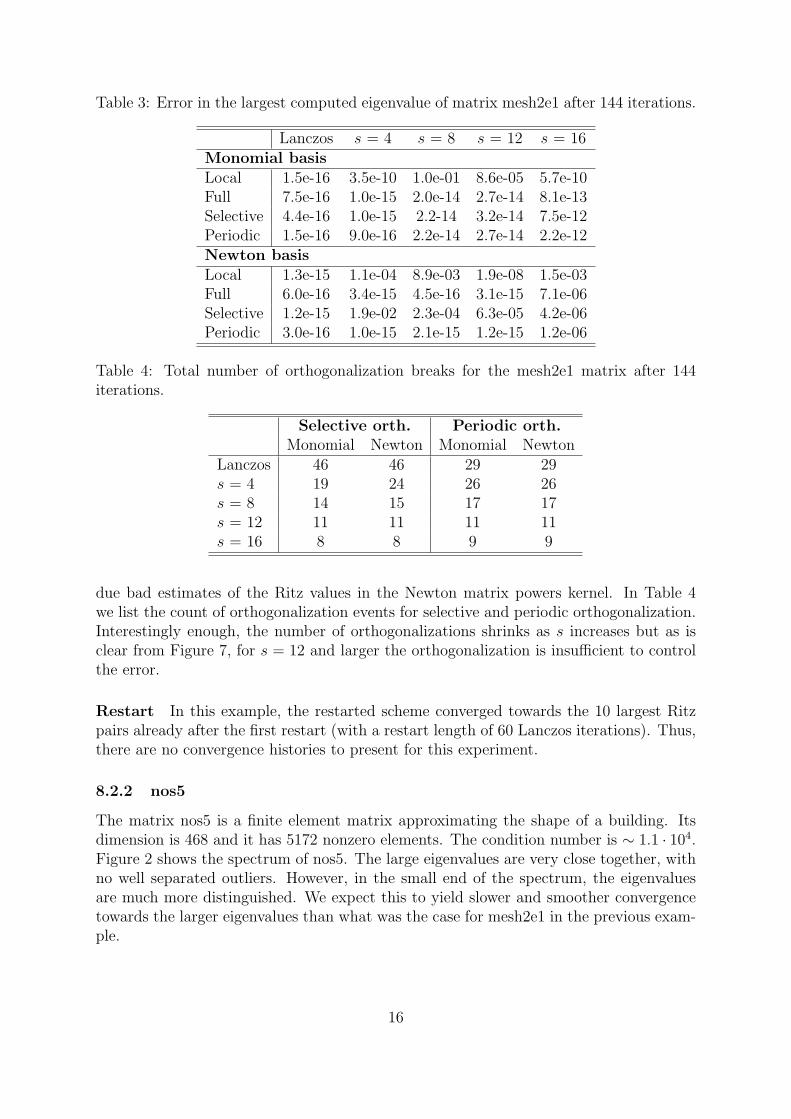
Table 3: Error in the largest computed eigenvalue of matrix mesh2e1 after 144 iterations.

Lanczos s = 4 s = 8 s = 12 s = 16Monomial basisLocal 1.5e-16 3.5e-10 1.0e-01 8.6e-05 5.7e-10Full 7.5e-16 1.0e-15 2.0e-14 2.7e-14 8.1e-13Selective 4.4e-16 1.0e-15 2.2-14 3.2e-14 7.5e-12Periodic 1.5e-16 9.0e-16 2.2e-14 2.7e-14 2.2e-12Newton basisLocal 1.3e-15 1.1e-04 8.9e-03 1.9e-08 1.5e-03Full 6.0e-16 3.4e-15 4.5e-16 3.1e-15 7.1e-06Selective 1.2e-15 1.9e-02 2.3e-04 6.3e-05 4.2e-06Periodic 3.0e-16 1.0e-15 2.1e-15 1.2e-15 1.2e-06

Table 4: Total number of orthogonalization breaks for the mesh2e1 matrix after 144iterations.

Selective orth. Periodic orth.Monomial Newton Monomial Newton

Lanczos 46 46 29 29s = 4 19 24 26 26s = 8 14 15 17 17s = 12 11 11 11 11s = 16 8 8 9 9

due bad estimates of the Ritz values in the Newton matrix powers kernel. In Table 4we list the count of orthogonalization events for selective and periodic orthogonalization.Interestingly enough, the number of orthogonalizations shrinks as s increases but as isclear from Figure 7, for s = 12 and larger the orthogonalization is insufficient to controlthe error.

Restart In this example, the restarted scheme converged towards the 10 largest Ritzpairs already after the first restart (with a restart length of 60 Lanczos iterations). Thus,there are no convergence histories to present for this experiment.

8.2.2 nos5

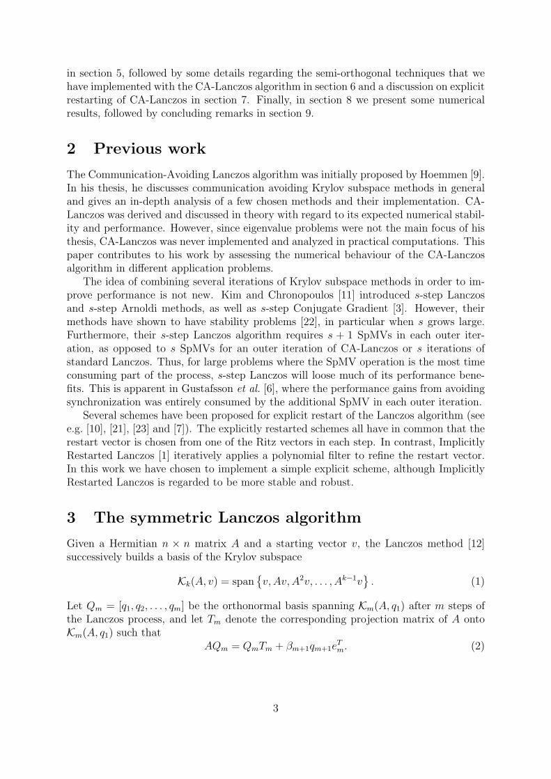
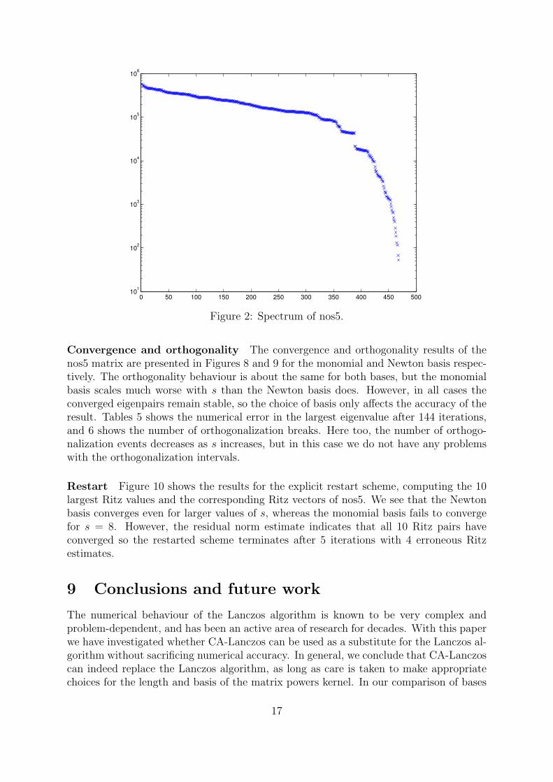
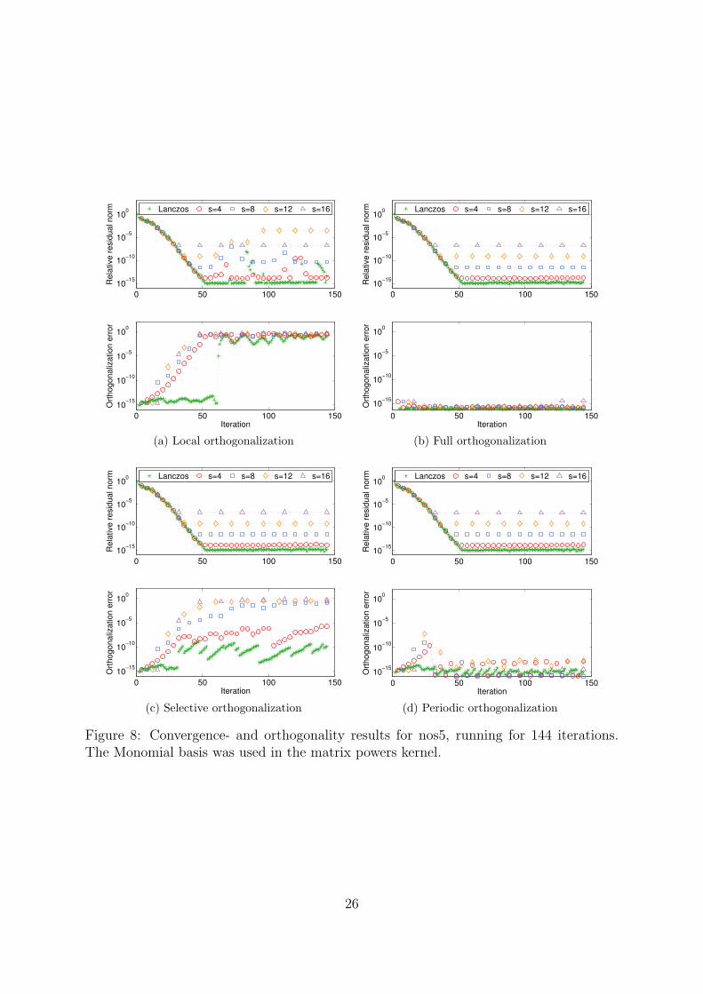
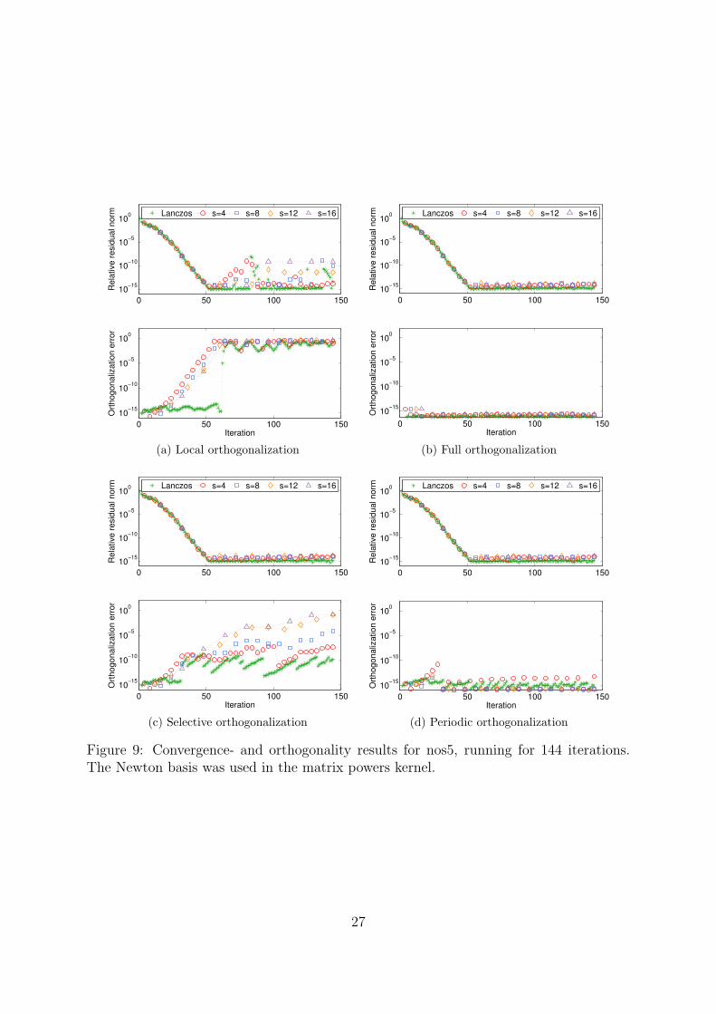
The matrix nos5 is a finite element matrix approximating the shape of a building. Itsdimension is 468 and it has 5172 nonzero elements. The condition number is ∼ 1.1 · 104.Figure 2 shows the spectrum of nos5. The large eigenvalues are very close together, withno well separated outliers. However, in the small end of the spectrum, the eigenvaluesare much more distinguished. We expect this to yield slower and smoother convergencetowards the larger eigenvalues than what was the case for mesh2e1 in the previous exam-ple.

16

0 50 100 150 200 250 300 350 400 450 50010

1

102

103

104

105

106

Figure 2: Spectrum of nos5.

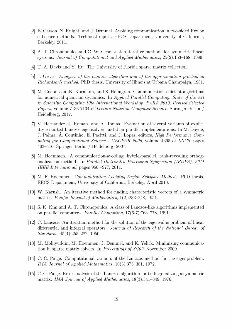
Convergence and orthogonality The convergence and orthogonality results of thenos5 matrix are presented in Figures 8 and 9 for the monomial and Newton basis respec-tively. The orthogonality behaviour is about the same for both bases, but the monomialbasis scales much worse with s than the Newton basis does. However, in all cases theconverged eigenpairs remain stable, so the choice of basis only affects the accuracy of theresult. Tables 5 shows the numerical error in the largest eigenvalue after 144 iterations,and 6 shows the number of orthogonalization breaks. Here too, the number of orthogo-nalization events decreases as s increases, but in this case we do not have any problemswith the orthogonalization intervals.

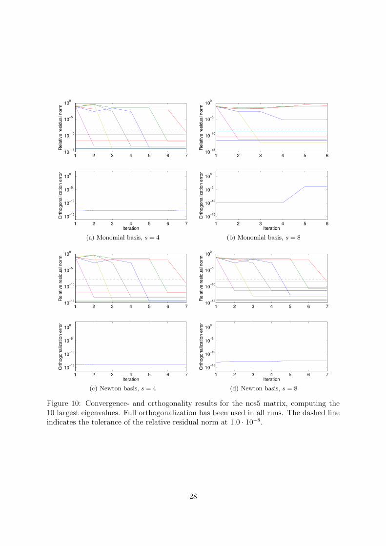
Restart Figure 10 shows the results for the explicit restart scheme, computing the 10largest Ritz values and the corresponding Ritz vectors of nos5. We see that the Newtonbasis converges even for larger values of s, whereas the monomial basis fails to convergefor s = 8. However, the residual norm estimate indicates that all 10 Ritz pairs haveconverged so the restarted scheme terminates after 5 iterations with 4 erroneous Ritzestimates.

9 Conclusions and future work

The numerical behaviour of the Lanczos algorithm is known to be very complex andproblem-dependent, and has been an active area of research for decades. With this paperwe have investigated whether CA-Lanczos can be used as a substitute for the Lanczos al-gorithm without sacrificing numerical accuracy. In general, we conclude that CA-Lanczoscan indeed replace the Lanczos algorithm, as long as care is taken to make appropriatechoices for the length and basis of the matrix powers kernel. In our comparison of bases

17

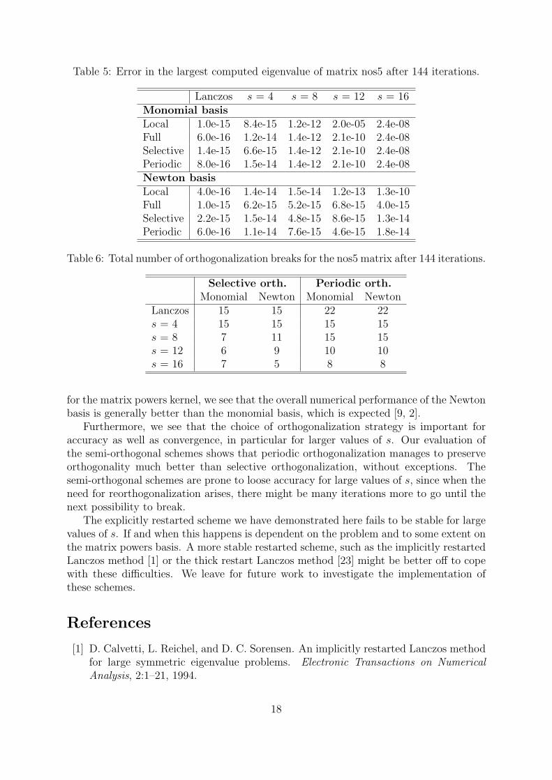
Table 5: Error in the largest computed eigenvalue of matrix nos5 after 144 iterations.

Lanczos s = 4 s = 8 s = 12 s = 16Monomial basisLocal 1.0e-15 8.4e-15 1.2e-12 2.0e-05 2.4e-08Full 6.0e-16 1.2e-14 1.4e-12 2.1e-10 2.4e-08Selective 1.4e-15 6.6e-15 1.4e-12 2.1e-10 2.4e-08Periodic 8.0e-16 1.5e-14 1.4e-12 2.1e-10 2.4e-08Newton basisLocal 4.0e-16 1.4e-14 1.5e-14 1.2e-13 1.3e-10Full 1.0e-15 6.2e-15 5.2e-15 6.8e-15 4.0e-15Selective 2.2e-15 1.5e-14 4.8e-15 8.6e-15 1.3e-14Periodic 6.0e-16 1.1e-14 7.6e-15 4.6e-15 1.8e-14

Table 6: Total number of orthogonalization breaks for the nos5 matrix after 144 iterations.

Selective orth. Periodic orth.Monomial Newton Monomial Newton

Lanczos 15 15 22 22s = 4 15 15 15 15s = 8 7 11 15 15s = 12 6 9 10 10s = 16 7 5 8 8

for the matrix powers kernel, we see that the overall numerical performance of the Newtonbasis is generally better than the monomial basis, which is expected [9, 2].

Furthermore, we see that the choice of orthogonalization strategy is important foraccuracy as well as convergence, in particular for larger values of s. Our evaluation ofthe semi-orthogonal schemes shows that periodic orthogonalization manages to preserveorthogonality much better than selective orthogonalization, without exceptions. Thesemi-orthogonal schemes are prone to loose accuracy for large values of s, since when theneed for reorthogonalization arises, there might be many iterations more to go until thenext possibility to break.

The explicitly restarted scheme we have demonstrated here fails to be stable for largevalues of s. If and when this happens is dependent on the problem and to some extent onthe matrix powers basis. A more stable restarted scheme, such as the implicitly restartedLanczos method [1] or the thick restart Lanczos method [23] might be better off to copewith these difficulties. We leave for future work to investigate the implementation ofthese schemes.

References

[1] D. Calvetti, L. Reichel, and D. C. Sorensen. An implicitly restarted Lanczos methodfor large symmetric eigenvalue problems. Electronic Transactions on NumericalAnalysis, 2:1–21, 1994.

18

[2] E. Carson, N. Knight, and J. Demmel. Avoiding communication in two-sided Krylovsubspace methods. Technical report, EECS Department, University of California,Berkeley, 2011.

[3] A. T. Chronopoulos and C. W. Gear. s-step iterative methods for symmetric linearsystems. Journal of Computational and Applied Mathematics, 25(2):153–168, 1989.

[4] T. A. Davis and Y. Hu. The University of Florida sparse matrix collection.

[5] J. Grcar. Analyses of the Lanczos algorithm and of the approximation problem inRichardson’s method. PhD thesis, University of Illinois at Urbana Champaign, 1981.

[6] M. Gustafsson, K. Kormann, and S. Holmgren. Communication-efficient algorithmsfor numerical quantum dynamics. In Applied Parallel Computing. State of the Artin Scientific Computing 10th International Workshop, PARA 2010, Revised SelectedPapers, volume 7133-7134 of Lecture Notes in Computer Science. Springer Berlin /Heidelberg, 2012.

[7] V. Hernandez, J. Roman, and A. Tomas. Evaluation of several variants of explic-itly restarted Lanczos eigensolvers and their parallel implementations. In M. Dayde,J. Palma, A. Coutinho, E. Pacitti, and J. Lopes, editors, High Performance Com-puting for Computational Science - VECPAR 2006, volume 4395 of LNCS, pages403–416. Springer Berlin / Heidelberg, 2007.

[8] M. Hoemmen. A communication-avoiding, hybrid-parallel, rank-revealing orthog-onalization method. In Parallel Distributed Processing Symposium (IPDPS), 2011IEEE International, pages 966 –977, 2011.

[9] M. F. Hoemmen. Communication-Avoiding Krylov Subspace Methods. PhD thesis,EECS Department, University of California, Berkeley, April 2010.

[10] W. Karush. An iterative method for finding characteristic vectors of a symmetricmatrix. Pacific Journal of Mathematics, 1(2):233–248, 1951.

[11] S. K. Kim and A. T. Chronopoulos. A class of Lanczos-like algorithms implementedon parallel computers. Parallel Computing, 17(6-7):763–778, 1991.

[12] C. Lanczos. An iteration method for the solution of the eigenvalue problem of lineardifferential and integral operators. Journal of Research of the National Bureau ofStandards, 45(4):255–282, 1950.

[13] M. Mohiyuddin, M. Hoemmen, J. Demmel, and K. Yelick. Minimizing communica-tion in sparse matrix solvers. In Proceedings of SC09, November 2009.

[14] C. C. Paige. Computational variants of the Lanczos method for the eigenproblem.IMA Journal of Applied Mathematics, 10(3):373–381, 1972.

[15] C. C. Paige. Error analysis of the Lanczos algorithm for tridiagonalizing a symmetricmatrix. IMA Journal of Applied Mathematics, 18(3):341–349, 1976.

19

[16] B. N. Parlett and D. S. Scott. The Lanczos algorithm with selective orthogonaliza-tion. Mathematics of Computation, 33(145):217–238, 1979.

[17] A. Ruhe. Lanczos method. In Z. Bai, J. Demmel, J. Dongarra, A. Ruhe, andH. van der Vorst, editors, Templates for the Solution of Algebraic Eigenvalue Prob-lems: A Practical Guide. SIAM, Philadelphia, 2000.

[18] H. D. Simon. Analysis of the symmetric Lanczos algorithm with reorthogonalizationmethods. Linear Algebra and its Applications, 61:101–131, 1984.

[19] H. D. Simon. The Lanczos algorithm with partial reorthogonalization. Mathematicsof Computation, 42(165):115–142, 1984.

[20] G. W. Stewart. Block Gram-Schmidt orthogonalization. SIAM Journal on ScientificComputing, 31(1):761–775, 2008.

[21] M. Szularz, J. Weston, and M. Clint. Explicitly restarted Lanczos algorithms in anMPP environment. Parallel Computing, 25(5):613–631, 1999.

[22] H. A. van der Vorst. Iterative Krylov Methods for Large Linear Systems. CambridgeUniversity Press, 2003.

[23] K. Wu and S. Horst. Thick-restart Lanczos method for large symmetric eigenvalueproblems. SIAM Journal on Matrix Analysis and Applications, 22(2):602–616, 2000.

20

0 100 200 300 400 500

10−15

10−10

10−5

100

Re

lative

re

sid

ua

l n

orm

Lanczos s=4 s=8 s=12 s=16

0 100 200 300 400 500

10−15

10−10

10−5

100

Ort

ho

go

na

liza

tio

n e

rro

r

Iteration

(a) Local orthogonalization

0 100 200 300 400 500

10−15

10−10

10−5

100

Re

lative

re

sid

ua

l n

orm

Lanczos s=4 s=8 s=12 s=16

0 100 200 300 400 500

10−15

10−10

10−5

100

Ort

ho

go

na

liza

tio

n e

rro

r

Iteration

(b) Full orthogonalization

0 100 200 300 400 500

10−15

10−10

10−5

100

Re

lative

re

sid

ua

l n

orm

Lanczos s=4 s=8 s=12 s=16

0 100 200 300 400 500

10−15

10−10

10−5

100

Ort

ho

go

na

liza

tio

n e

rro

r

Iteration

(c) Selective orthogonalization

0 100 200 300 400 500

10−15

10−10

10−5

100

Re

lative

re

sid

ua

l n

orm

Lanczos s=4 s=8 s=12 s=16

0 100 200 300 400 500

10−15

10−10

10−5

100

Ort

ho

go

na

liza

tio

n e

rro

r

Iteration

(d) Periodic orthogonalization

Figure 3: Convergence- and orthogonality results for a 500 × 500 diagonal matrix withcondition number 100, running for 480 iterations. The Monomial basis was used in thematrix powers kernel.

21

0 100 200 300 400 500

10−15

10−10

10−5

100

Re

lative

re

sid

ua

l n

orm

Lanczos s=4 s=8 s=12 s=16

0 100 200 300 400 500

10−15

10−10

10−5

100

Ort

ho

go

na

liza

tio

n e

rro

r

Iteration

(a) Local orthogonalization

0 100 200 300 400 500

10−15

10−10

10−5

100

Re

lative

re

sid

ua

l n

orm

Lanczos s=4 s=8 s=12 s=16

0 100 200 300 400 500

10−15

10−10

10−5

100

Ort

ho

go

na

liza

tio

n e

rro

r

Iteration

(b) Full orthogonalization

0 100 200 300 400 500

10−15

10−10

10−5

100

Re

lative

re

sid

ua

l n

orm

Lanczos s=4 s=8 s=12 s=16

0 100 200 300 400 500

10−15

10−10

10−5

100

Ort

ho

go

na

liza

tio

n e

rro

r

Iteration

(c) Selective orthogonalization

0 100 200 300 400 500

10−15

10−10

10−5

100

Re

lative

re

sid

ua

l n

orm

Lanczos s=4 s=8 s=12 s=16

0 100 200 300 400 500

10−15

10−10

10−5

100

Ort

ho

go

na

liza

tio

n e

rro

r

Iteration

(d) Periodic orthogonalization

Figure 4: Convergence- and orthogonality results for a 500 × 500 diagonal matrix withcondition number 100, running for 480 iterations. The Newton basis was used in thematrix powers kernel.

22

0 20 40 60 80 10010

−10

10−5

100

Re

lative

re

sid

ua

l n

orm

0 20 40 60 80 100

10−15

10−10

10−5

100

Iteration

Ort

ho

go

na

liza

tio

n e

rro

r

(a) Monomial basis, s = 4

0 20 40 60 80 10010

−10

10−5

100

Re

lative

re

sid

ua

l n

orm

0 20 40 60 80 100

10−15

10−10

10−5

100

Iteration

Ort

ho

go

na

liza

tio

n e

rro

r

(b) Monomial basis, s = 8

0 20 40 60 80 10010

−10

10−5

100

Re

lative

re

sid

ua

l n

orm

0 20 40 60 80 100

10−15

10−10

10−5

100

Iteration

Ort

ho

go

na

liza

tio

n e

rro

r

(c) Newton basis, s = 4

0 20 40 60 80 10010

−10

10−5

100

Re

lative

re

sid

ua

l n

orm

0 20 40 60 80 100

10−15

10−10

10−5

100

Iteration

Ort

ho

go

na

liza

tio

n e

rro

r

(d) Newton basis, s = 12

Figure 5: Convergence- and orthogonality results for a 5000× 5000 diagonal matrix withcondition number 1.0 · 104, computing the 10 largest eigenvalues. Full orthogonalizationhas been used in all runs. The dashed line indicates the tolerance of the relative residualnorm at 1.0 · 10−8.

23

0 50 100 150

10−15

10−10

10−5

100

Re

lative

re

sid

ua

l n

orm

Lanczos s=4 s=8 s=12 s=16

0 50 100 150

10−15

10−10

10−5

100

Ort

ho

go

na

liza

tio

n e

rro

r

Iteration

(a) Local orthogonalization

0 50 100 150

10−15

10−10

10−5

100

Re

lative

re

sid

ua

l n

orm

Lanczos s=4 s=8 s=12 s=16

0 50 100 150

10−15

10−10

10−5

100

Ort

ho

go

na

liza

tio

n e

rro

r

Iteration

(b) Full orthogonalization

0 50 100 150

10−15

10−10

10−5

100

Re

lative

re

sid

ua

l n

orm

Lanczos s=4 s=8 s=12 s=16

0 50 100 150

10−15

10−10

10−5

100

Ort

ho

go

na

liza

tio

n e

rro

r

Iteration

(c) Selective orthogonalization

0 50 100 150

10−15

10−10

10−5

100

Re

lative

re

sid

ua

l n

orm

Lanczos s=4 s=8 s=12 s=16

0 50 100 150

10−15

10−10

10−5

100

Ort

ho

go

na

liza

tio

n e

rro

r

Iteration

(d) Periodic orthogonalization

Figure 6: Convergence- and orthogonality results for mesh2e1, running for 144 iterations.The Monomial basis was used in the matrix powers kernel.

24

0 50 100 150

10−15

10−10

10−5

100

Re

lative

re

sid

ua

l n

orm

Lanczos s=4 s=8 s=12 s=16

0 50 100 150

10−15

10−10

10−5

100

Ort

ho

go

na

liza

tio

n e

rro

r

Iteration

(a) Local orthogonalization

0 50 100 150

10−15

10−10

10−5

100

Re

lative

re

sid

ua

l n

orm

Lanczos s=4 s=8 s=12 s=16

0 50 100 150

10−15

10−10

10−5

100

Ort

ho

go

na

liza

tio

n e

rro

r

Iteration

(b) Full orthogonalization

0 50 100 150

10−15

10−10

10−5

100

Re

lative

re

sid

ua

l n

orm

Lanczos s=4 s=8 s=12 s=16

0 50 100 150

10−15

10−10

10−5

100

Ort

ho

go

na

liza

tio

n e

rro

r

Iteration

(c) Selective orthogonalization

0 50 100 150

10−15

10−10

10−5

100

Re

lative

re

sid

ua

l n

orm

Lanczos s=4 s=8 s=12 s=16

0 50 100 150

10−15

10−10

10−5

100

Ort

ho

go

na

liza

tio

n e

rro

r

Iteration

(d) Periodic orthogonalization

Figure 7: Convergence- and orthogonality results for mesh2e1, running for 144 iterations.The Newton basis was used in the matrix powers kernel.

25

0 50 100 150

10−15

10−10

10−5

100

Re

lative

re

sid

ua

l n

orm

Lanczos s=4 s=8 s=12 s=16

0 50 100 150

10−15

10−10

10−5

100

Ort

ho

go

na

liza

tio

n e

rro

r

Iteration

(a) Local orthogonalization

0 50 100 150

10−15

10−10

10−5

100

Re

lative

re

sid

ua

l n

orm

Lanczos s=4 s=8 s=12 s=16

0 50 100 150

10−15

10−10

10−5

100

Ort

ho

go

na

liza

tio

n e

rro

r

Iteration

(b) Full orthogonalization

0 50 100 150

10−15

10−10

10−5

100

Re

lative

re

sid

ua

l n

orm

Lanczos s=4 s=8 s=12 s=16

0 50 100 150

10−15

10−10

10−5

100

Ort

ho

go

na

liza

tio

n e

rro

r

Iteration

(c) Selective orthogonalization

0 50 100 150

10−15

10−10

10−5

100

Re

lative

re

sid

ua

l n

orm

Lanczos s=4 s=8 s=12 s=16

0 50 100 150

10−15

10−10

10−5

100

Ort

ho

go

na

liza

tio

n e

rro

r

Iteration

(d) Periodic orthogonalization

Figure 8: Convergence- and orthogonality results for nos5, running for 144 iterations.The Monomial basis was used in the matrix powers kernel.

26

0 50 100 150

10−15

10−10

10−5

100

Re

lative

re

sid

ua

l n

orm

Lanczos s=4 s=8 s=12 s=16

0 50 100 150

10−15

10−10

10−5

100

Ort

ho

go

na

liza

tio

n e

rro

r

Iteration

(a) Local orthogonalization

0 50 100 150

10−15

10−10

10−5

100

Re

lative

re

sid

ua

l n

orm

Lanczos s=4 s=8 s=12 s=16

0 50 100 150

10−15

10−10

10−5

100

Ort

ho

go

na

liza

tio

n e

rro

r

Iteration

(b) Full orthogonalization

0 50 100 150

10−15

10−10

10−5

100

Re

lative

re

sid

ua

l n

orm

Lanczos s=4 s=8 s=12 s=16

0 50 100 150

10−15

10−10

10−5

100

Ort

ho

go

na

liza

tio

n e

rro

r

Iteration

(c) Selective orthogonalization

0 50 100 150

10−15

10−10

10−5

100

Re

lative

re

sid

ua

l n

orm

Lanczos s=4 s=8 s=12 s=16

0 50 100 150

10−15

10−10

10−5

100

Ort

ho

go

na

liza

tio

n e

rro

r

Iteration

(d) Periodic orthogonalization

Figure 9: Convergence- and orthogonality results for nos5, running for 144 iterations.The Newton basis was used in the matrix powers kernel.

27

1 2 3 4 5 6 710

−15

10−10

10−5

100

Rela

tive r

esid

ual norm

1 2 3 4 5 6 7

10−15

10−10

10−5

100

Iteration

Ort

hogonaliz

ation e

rror

(a) Monomial basis, s = 4

1 2 3 4 5 610

−15

10−10

10−5

100

Rela

tive r

esid

ual norm

1 2 3 4 5 6

10−15

10−10

10−5

100

Iteration

Ort

hogonaliz

ation e

rror

(b) Monomial basis, s = 8

1 2 3 4 5 6 710

−15

10−10

10−5

100

Rela

tive r

esid

ual norm

1 2 3 4 5 6 7

10−15

10−10

10−5

100

Iteration

Ort

hogonaliz

ation e

rror

(c) Newton basis, s = 4

1 2 3 4 5 6 710

−15

10−10

10−5

100

Rela

tive r

esid

ual norm

1 2 3 4 5 6 7

10−15

10−10

10−5

100

Iteration

Ort

hogonaliz

ation e

rror

(d) Newton basis, s = 8

Figure 10: Convergence- and orthogonality results for the nos5 matrix, computing the10 largest eigenvalues. Full orthogonalization has been used in all runs. The dashed lineindicates the tolerance of the relative residual norm at 1.0 · 10−8.

28