A Look-Ahead Lanczos Algorithm - AMS

MATHEMATICS OF COMPUTATIONVOLUME 44, NUMBER 169JANUARY 1985, PAGES 105-124

A Look-Ahead Lanczos Algorithm

for Unsymmetric Matrices

By Beresford N. Parlett, Derek R. Taylor and Zhishun A. Liu*

Abstract. The two-sided Lanczos algorithm sometimes suffers from serious breakdowns. These

occur when the associated moment matrix does not permit triangular factorization. We

modify the algorithm slightly so that it corresponds to using a 2 X 2 pivot in triangular

factorization whenever a 1 x 1 pivot would be dangerous. The likelihood of breakdown is

greatly reduced. The price paid is that the tridiagonal matrix produced by the algorithm now

has bumps whenever a 2 X 2 pivot is used. Experiments with several versions of the algorithm

on a variety of matrices are described, including some large problems arising in the study of

plasma instability.

1. The Lanczos Algorithm and Its Breakdown. The most popular way to obtain all

the eigenvalues of a nonsymmetric « X n matrix B is to use the QR algorithm which

is readily available in most computing centers. As the order n increases above 100

the QR algorithm becomes less and less attractive, especially if only a few of the

eigenvalues are wanted. This is where the Lanczos algorithm comes into the picture.

It does not alter B at all but constructs a tridiagonal matrix J gradually by adding a

row and column at each step. After several steps some of the eigenvalues 6¡ of / will

be close to some eigenvalues Xk of B and by the nth step, if nothing goes wrong,

6¡ = \¡, i = l,...,n. This description is correct in the context of exact arithmetic.

Unfortunately things can go wrong, even in the absence of rounding errors. The

relations between these troubles and orthogonal polynomials are developed in [2].

In order to discuss these troubles we must say more about the algorithm. Let Jk be

the k X k tridiagonal produced at step k of the algorithm. There are infinitely many

tridiagonal matrices similar to B and Jn is one of them. Thus for some matrix

Q„:= iqx,...,qn) we have

(1) Q;lBQn = J„.

It simplifies the exposition considerably to introduce a redundant symbol and write

P* instead of Q~l. The superscript * indicates conjugate transpose.

Let P„:= ipx,...,pn) and replace(1) by two separate relations

(2) p:q„ = /,

Received July 6, 1981; revised March 6, 1984.

1980 Mathematics Subject Classification. Primary 65F15.

The first and third authors gratefully acknowledge.support by the Office of Naval Research under

Contract N00014-76-C-0013. The second author thanks the Remote Sensing program at the University of

California, Berkeley, for use of its computer facility.

©1985 American Mathematical Society

0025-5718/85 $1.00 + $.25 per page

105

License or copyright restrictions may apply to redistribution; see https://www.ams.org/journal-terms-of-use

106 BERESFORD N. PARLETT, DEREK R. TAYLOR AND ZHISHUN A. LIU

(3) Pn*BnQn = Jn.

We mention in passing that when B* = B = A, then we can arrange that P„ = Qn.

The difficulty we are going to describe cannot occur when Pn = Q„.

By equating elements on each side of BQ„ = Q„J„ and P*B = JnP* in the natural

increasing order, we shall see that B, px and qx essentially determine all the other

elements of P„, Q„ and Jn. On writing

J-=

p\

Y2

03

Y3

AJn

a„

we find

and

p*Bqx = a,,

#4i - 9i«i + 92Ä, />*£ = a^ï + y2p^.

Hence #2 and/>* are> respectively, multiples of "residual" vectors

r2:= 5^ -?!«!, := p\B - axp*.

Furthermore, since p\q2 = 1 by (2), we have

s*r2 = yiPiQißi = yißi '■= «2.

If w2 ¥= 0 and /?2 is given any nonzero value, then y2, q2 and p* are all determined

uniquely. One good choice is ß2 = ^|<o2|.

The general pattern emerges at the next step, on equating the second columns on

each side of BQ„ = QnJn and P¿B = JnP„*,

p\Bq2 = a2,

Ba2 = 1lY2 + ?2«2 + ?303' P*B = ßiP* + a2P* + KP*-

At this point we can compute the " residual" vectors

r3 := Bq2 - qxy2 - q2a2, i3* := p\B - ß2p\ - a2p\

and

<o3:= s3*r3 = y3ß3.

If u3 ^ 0 and ß3 is given any nonzero value then y3, q3 and p* are all determined

uniquely. And so it goes on until some Oj vanishes.

Example 1 (No breakdown).

5 = diag(2,3,4), if-HLLI]. PÎ-H1.2.1].

Step I:

Step 2:

ax = 3, «2 = i

«î-H-i.0,1],

a2 = 3, w3 = i,

??-Hi.-i.i].

02=1. Y2 = ï-

PÎ-[-1,0,1].

03 = 1. Y3 = Í

i»í-Hi,-2,i].


A LANCZOS ALGORITHM FOR UNSYMMETRIC MATRICES 107

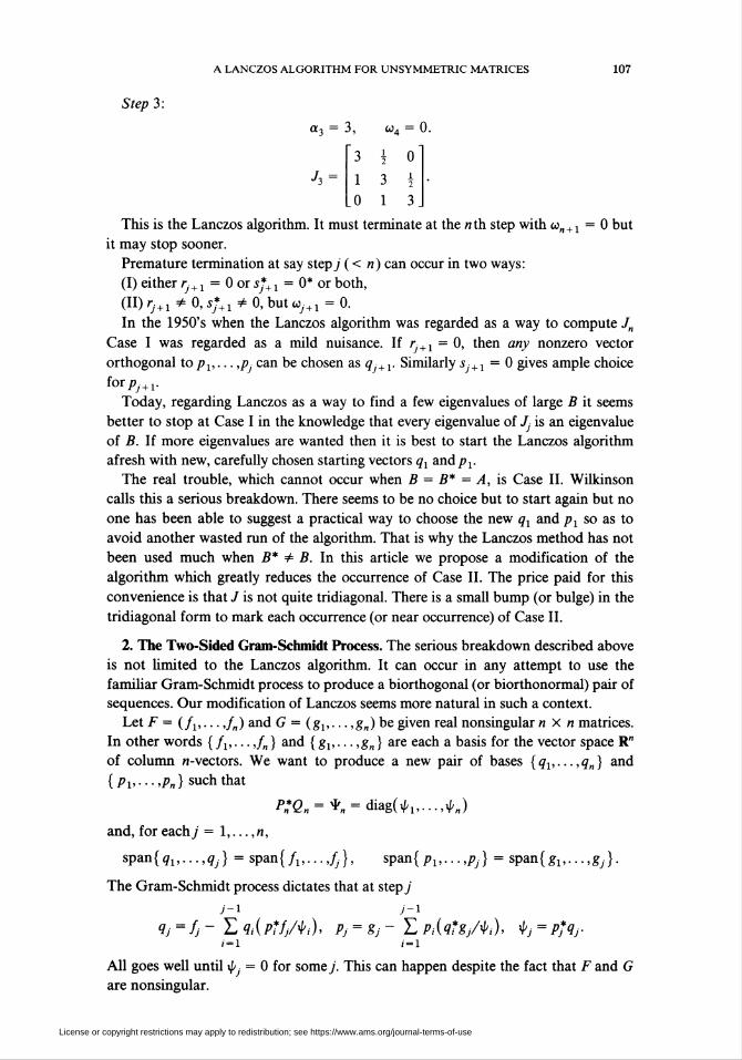
Step 3:

a3 = 3, «4 = 0'3 * (

J, 1 3 §

.0 1 3

This is the Lanczos algorithm. It must terminate at the nth step with w„+1 = 0 but

it may stop sooner.

Premature termination at say step y (< n) can occur in two ways:

(I) either rj+x = 0 or sj+x = 0* or both,

(II) rj+x ¥> 0, s*+x * 0, but oJ+1 = 0.

In the 1950's when the Lanczos algorithm was regarded as a way to compute Jn

Case I was regarded as a mild nuisance. If rj+x = 0, then any nonzero vector

orthogonal to />,,... ,pj can be chosen as qj+x. Similarly sJ+x = 0 gives ample choice

for pj+l.

Today, regarding Lanczos as a way to find a few eigenvalues of large B it seems

better to stop at Case I in the knowledge that every eigenvalue of Jj is an eigenvalue

of B. If more eigenvalues are wanted then it is best to start the Lanczos algorithm

afresh with new, carefully chosen starting vectors qx and/^.

The real trouble, which cannot occur when B = B* = A, is Case II. Wilkinson

calls this a serious breakdown. There seems to be no choice but to start again but no

one has been able to suggest a practical way to choose the new qx and px so as to

avoid another wasted run of the algorithm. That is why the Lanczos method has not

been used much when B* ± B. In this article we propose a modification of the

algorithm which greatly reduces the occurrence of Case II. The price paid for this

convenience is that J is not quite tridiagonal. There is a small bump (or bulge) in the

tridiagonal form to mark each occurrence (or near occurrence) of Case II.

2. The Two-Sided Gram-Schmidt Process. The serious breakdown described above

is not limited to the Lanczos algorithm. It can occur in any attempt to use the

familiar Gram-Schmidt process to produce a biorthogonal (or biorthonormal) pair of

sequences. Our modification of Lanczos seems more natural in such a context.

Let F = ifx,...,f„) and G = (g,,... ,g„) be given real nonsingular n X n matrices.

In other words { /,, ...,/„} and {gx,.--,g„} are each a basis for the vector space R"

of column «-vectors. We want to produce a new pair of bases {qx,...,qn} and

{Pv■•■>Pn) suchthat

and, for each y = 1,...,«,

span{qx,...,qj} = spm{fl,...,fj}, span{/>,,...,/>,} = span{gx,...,gy}.

The Gram-Schmidt process dictates that at step y

7-1 7-1

aj = fj- Z<i,{ptfj/ti), Pj = Sj- LPiiih/ti), tj = p*<ij-i=i /=i

All goes well until \pj = 0 for some/ This can happen despite the fact that F and G

are nonsingular.



Example 2.

F =1 12 11 2

1 1 10 0 10 1 0

Stepl:qx =fx,px = gx,i>x = 1.

Step 2: q* = [0,1,0], p* - [-1,0,1], *2 = 0.

Our remedy for the case i^ = 0 is quite natural. If pj =£ 0 then recompute qj using

fj+x in place of fj. If this fails too, then try fJ+2, and so on. If Fis nonsingular, there

must be some i > 0 such that^+, will yield a nonzero value for i^.

Here is a formai proof of the last remarks. Let qj(k) denote the vector obtained by

using/j. instead of fj, i.e.,

7-1

q)k) = fk- ZqÂPÎMi)-

Lemma. Ifpj =£ 0 andp*q{jk) = Ofor k = j, j + l,...,n, then F is singular.

Proof. By construction/^*^, = 0 for i <j.

Hence pj 1 span(/,,...,/,_,).

Thus 0 = p*q)k) = p*fk - 0, for all k > j.

Thus/»,. ± span(/,,...,/„).

Thus pj*F = 0 and F is singular. D

Now consider again the use of fj+x instead of fj. If the modification succeeds the

first time then only one property of Gram-Schmidt has been sacrificed, namely

span(?!,...,4y) # span(/j,...,/y).

Moreover, if no further breakdown occurs then

span(<?!,...,?,.) = span(/1;...,y;) for/ >y.

In many applications this price is well worth paying. Before describing our remedy

we must relate Gram-Schmidt to Lanczos.

The Lanczos algorithm can be regarded as the two-sided Gram-Schmidt process

applied to the columns of the special matrices

K=Kn:=[qx,Bqx,B2qx,...,B"-\\, and K* = K*n

P\

p\B

p*B2

p*xB-i

We will not establish this result but content ourselves with stating the key observa-

tion, namely

span(ft, q2,.. .,q}, Bq;) = span(^,.. .,qJt ßjqx).

The K matrices are called Krylov matrices and the pleasant fact is that most of the

work required for general Gram-Schmidt disappears in this case because

p*Bqj = 0 for/< y-1.



Thus, the general formula

7

ßj+iqj+i = Bjqx- Zl.ipfB^/^)i = l

collapses to the famous three-term recurrence

ßj+tfj+i = H - 1j«j - Ij-îtj-v

3. Triangular Factorization of Moment Matrices. Consider again the matrices K

and K* defined in the previous section. Note that the (/, j) element of K*K is

(pïB'-^iBJ-^), so

K*K=M = M(px,qx); where mi+hj+x = p\B'+Jqx.

In order to use this observation we need some basic facts about the Lanczos

algorithm (see [3], [5] or [12]). If it does not break down it produces matrices P and Q

such that

qJ+i = xj(B)qx/I rul pj+i = xj(b*)pi/in?,.

where

Xj+M = (t - aj)Xj(t) - UjXj-i(t),

and Xj is the characteristic polynomial of the tridiagonal matrix J}. In other words,

for eachy, q^ is a linear combination of the first j columns of K while pj is the same

linear combination of the columns of K, up to scaling. This can be expressed

compactly in matrix notation as

(4) Q = KL~*U-\ P = KL-*n-\

Here

IT = diag(l, ß2, ß2ß3,...), IT = diag(l, y2, y2y3,...),

and L is the unit lower triangular matrix such that L~* := (L-1)* has the coeffi-

cients of Xj above the diagonal in they th column.

Using (4) we can rewrite / = P*Q as

i = p*q = (ÜlL-1K*)(KL-*U~1),

i.e.,

(5) M = LQ.L*,

where

fi = Un = diag(l, w2, w2w3,..., <o2 • • • <o„ ).

This result is not new (see Householder [3]) but it is worth emphasizing that the

product <o2 • ■ • w, is the ith pivot used in performing Gaussian elimination on the

moment matrix M associated with B, qx and px.

When B ¥= B* the moment matrix M need not be positive definite and so

triangular factorization need not be stable, even when M is nonsingular. Even when

B* = B = A it is the condition qx = px which forces M to be positive definite.

The best known remedy when ||L|| » \\M|| is to use some form of row or column

interchange whenever an to, is too small. The standard " partial pivoting" strategy is



not available because a whole column of M is not available in the middle of the

Lanczos process. An alternative remedy is to enlarge the notion of a "pivot" to

include 2 X 2, or even larger submatrices. This idea is discussed in Parlett and

Bunch, 1971, [8]. It is the basis of our method. Whenever a 2 X 2 pivot is used the

tridiagonal J bulges outwards temporarily.

In the context of the Lanczos process, our remedy for a tiny Uj requires us to

compute qJ+x at the same time as qj, and pj+x at the same time as /»■. The formulas

for these " Lanczos" vectors are somewhat different from the standard ones. We call

our modification the "look-ahead Lanczos algorithm" because it computes at the

current step some quantities which are not usually needed until the next step in the

standard Lanczos process. However, no matrix-vector products Bq or p*B are ever

wasted.

4. The Next Pivot. The decomposition M = LQL* is never found explicitly. In

order to make use of the idea of using a 2 X 2 pivot it is necessary to determine the

top left 2x2 submatrix of what would be the reduced matrix in the triangular

factorization of M. These three numbers can be determined from the information

available in the Lanczos process.

After /' — 1 steps of the standard algorithm we have

ri:= Bq¡-i - ?,-i«,-i - î/-2Yi-i = X,-i(#)<7i/(02 • • • 0,-i),

s* := p*_xB - a^pU - ßi-1pt2=ptxi-i(B)/(y2 ■ ■ ■ y¡_x),

«,:= s*r¡.

Instead of normalizing r, and s* to get q¡ and p* we can look ahead not to the next

Lanczos vectors qi+x,pf+x but to any vectors ri+1, s*+x such that

the plane (r¡, rl+x) = the plane (q,, qi+x),

the plane (s*, sf+ x) = the plane ( p*, p*+ x).

The simplest choice for ri+x and si+ x is

ri+i '■= Br, - 9¿-r»/> 5*+i := stB - <*iP?-i-

The coefficient w, ensures that rj+x is orthogonal to all the known />'s, namely

px,... ,Pi_x, and also thats, + 1 is orthogonal to qx,.. .,q¡_x.

Note that if we choose as q¡ any vector in the plane (r„ ri+x) other than a multiple

of r¡ then q¡ will be of the form

q, = t(B)qx/(ß2--- ß.)

vith \¡> a monic polynomial of degree i instead of the usual x¡-i 0I degree / — 1.

Moreover, it will be possible to choose qi+x to be of the same form, using a different

\p but of the same degree /'. This is a mild generalization of the basic Lanczos

algorithm. The degrees of the new Lanczos polynomials are still nondecreasing but

they do not always go up by one at each step. Before making a choice for q¡, qi+x,pt,

pi+x we compute

||r,-||, ||i,||, and cosz(r,., S¡) = w,/||r,.|| • ||i*||.

Also,

wi + l = i/+lri+l> "i = si ri+\ = s/+lr/>

Ik+ill, Ikf+ill. cosZ(r,+1, si+x) = k+1|/||ri+1|| • ||jf+1||.



Our choice of q¡, etc., must be based on the matrix

"w, 6,W,= e, ui+i

It turns out that the top left 2x2 submatrix of the reduced matrix that occurs in

the associated triangular factorization of M is (co2 • • • co,.,)!^. The reduced matrix

is defined in [7, p. 198].

If both w, = 0 and W¡ is singular then more drastic measures are needed to salvage

the algorithm. We will pursue this case in Section 7. When w, = 0 then the standard

Lanczos algorithm breaks down. Yet, if Wi is invertible, it is easy to choose suitable

q 's and p 's so that the algorithm can proceed.

The equations above can be condensed into block form.

(r¡, ri+1) = B(q¡_x, r,) -(?,_!, r,)\*i-i

0 0 9/-2[Yí-i.0]>

(í/.í/ + l)* = (/>,-!> ■*,)*£-

0

w, ÍPt-u',)*-0,-1

0pr-2.

W,= (si,si+x)*(ri,ri+x)=:<o 6

0. a 1 + 1

Various factorizations of W¡ yield various selections for new q 's and p 's. These are

discussed below. We write cô for co,+1 and 0 for 6¡. Let us drop the subscript /' and

write

S*R= W= VU.

Rewrite the above equation as

/= V~lS*RU~l = (SV~*)*(RU1)

and recall that P*Q = I. We thus have

P = SV~*, Q = RU~l.

1. LU factorization

V =1 0

e/u iu =

w 6

0 w - 02/w

2. UL factorization

3. QR factorization

a - e2/û e

0 usu = 1 0

0/ù 1

(0 -f?v =

4. LU with interchange

V =

U =

us/6 1

1 0

t2 6(os + cô)

0 (coco-f?2)T"1, T = VV + ff2 .

i/'Ö CO

o ô - uCs/e

5. T/ie smallest angle. In order to determine the smallest angle between the planes

(r,, ri+x) and (s,, 5i+1) it is best to orthonormalize the bases. Let the result be

O/./i+i) a00 (j,.f/+i).



when the Gram-Schmidt process is used. The (matrix) angle between the two planes,

call it $, is defined, see [1], by

cos<D = (î,,g,+1)*(r„/ + 1).

Let the Singular Value Decomposition of cos 4> be

cos O = U1V*

where 2 = diag(a,, a2) and ox > a2. The appropriate definition of new Lanczos

vectors to ensure the smallest Z(q¡, p¡) is

(q„ ql+i) = in, /+1)K2-1/2, (p„ pi+x) = (s„ gi+1)U2-^2.

Comments on the Factorizations. No. 1 corresponds to the standard Lanczos

algorithm. No. 2 corresponds to simply swapping s* with s*B and r¡ with Brt in the

Lanczos algorithm. One consequence is that the J matrix will bulge out of tridiago-

nal form on both sides of the diagonal. No. 3 is always stable and keeps the bulge on

one side. The same advantage accrues from No. 4 and, as might be expected, is

somewhat simpler than No. 3.

We want to use No. 1 whenever this is a reasonable strategy but when co is zero or

very small it is vital to choose one of the other procedures. We have tentatively

chosen No. 4 on the grounds of simplicity. The interesting question which we now

address is when to use No. 4.

Initial success with No. 4 did not encourage us to implement No. 5. Then, in his

thesis [11], D. R. Taylor struck a fatal blow at the claims of No. 5. We summarize

the results in Section 3.5 here.

If Pj and q¡ are chosen to minimize z(p¡, q¡) then biorthonormality fixes pi+x and

qi+x and

cosz( Pi,qi) = ox = largest singular value of cos $,

cos z(pi+x,qi+x) = o2 — smallest singular value of cos O.

Now the best practical measure of the linear independence of the bases { px,... ,/>■}

and {qx,...,qj} is

max Z(pi,qi)i

or, more practically,

min cosZ( Pi, q¡).i

From this point of view the best choice at a double step is to maximize

ttán{cosz(pi,qi),cosz(pi+1,qí+í)}.

Clearly, No. 5 is a poor choice. Taylor proves (Theorem 3.1) that this maximum is

2oxo2/(ox + o2), the harmonic mean of ax and a2.

These results make precise the following intuitive picture. If Z(r¡, s¡) is large but

the planes spanned by (r¡, ri+x), (sitsi+1) are quite close to each other then our

modifications to Lanczos will pay off handsomely. If, however, one of the angles

between the planes is nearly a right angle then our device will not help.

Criterion for Choosing a 2 X 2 Pivot. When Factorization No. 4 is chosen then

(?/.9/+i) = (l. r,+i)i -<W4o i (PnPi+i) = (*<+!>■*/)

1 -«/*/

0 1



to within scalar multiples. Please note the interchange. Hence

0.cos49,, Pi) = cosZ(r,., i/+1) = -:+„

'i+ni

cosZ(qi+x,pi+x) =($i - co,co, + 1/0,.)

0, I -Q )i

= :4>i+V

Both these numbers are readily computable, without forming the new vectors,

provided that r*+xr¡ and s*+xs¡ are known. The choice between No. 1 and No. 4

reduces to a comparison of

</>! = |cosz(r,, s,)\ and <p2 = min{|i//,|, |i//,-+1|).

If <f>x < 100e and <p2 < lOOe then our algorithm stops and reports failure. Otherwise,

for a given bias factor we proceed as follows: if <¡>x > (bias factor)<>2 then use

standard Lanczos else use Factorization No. 4. When bias = 0 we recover the

standard algorithm. Currently bias = 2.

Sometimes the test declares that a standard Lanczos step is safe. In such cases, \¡/x

and \j/2 are not used and their computation may be regarded as an overhead of four

inner products. Fortunately no matrix-vector products are "wasted". The four inner

products arise as follows. We need

sr = SL f,H2-2Í|i|^ |ylK+il

w1+1

0,= \r<i+i |2-2M

i+i

0,r¡ r¡.

os;+i

0,

We may regard the second and third terms on the right-hand sides as the price to be

paid for knowing that a standard Lanczos step is safe. Observe that fi+l and s* are

not computed.

To summarize, let us write R¿ = (r,, rj+x), S¡ = (*„ si+x).

The look-ahead part of the algorithm comprises the computation of ri+x, si+x and

the unknown elements of S*R¡, R*R¡ and S*S¡. Before specifying the algorithm we

describe the bumpy tridiagonal matrix /.

5. /, The Projection of B. The standard (biorthogonal) Lanczos algorithm pro-

duces a tridiagonal matrix Jj by the end of step j. The look-ahead algorithm produces

a block tridiagonal matrix, also called J,, and written as

ax r2

B, r3

B,

B. AJ

The diagonal blocks are capital a's and the subdiagonal blocks are capital ß's. The

A i are either lxl or 2 X 2 and the B¡ and T, are shaped conformably. For



convenience in finding eigenvalues of J we have forced each 73, to have one of the

following four forms

[ + ]. [0 +],

where + stands for a positive quantity. It turns out that each T, also has rank one.

The left and right Lanczos vectors will be grouped by step and written as

Px*, P2*,.. .,Pj* and Qx,..., Qj, where sometimes Q¡ is « X 1 and sometimes n X 2.

We collect the vectors together in Q] = (Qx,. ..,Qj) and Pj = (i>1,...,P). The

matrix QjP* is the projector matrix onto the left and right Krylov subspaces and

B 's (oblique) projection into them is defined by

(Qjp;)b(QjP;) = QjjjP;.

Thus Jj is the representation of this projection with respect to the bases given by the

rows of P* and the columns of Q,.J x-7

Please note that y is not the order of Jj.

6. The Look-Ahead Lanczos Algorithm (called LAL hereafter). We have chosen our

notation to camouflage the complications caused by the fact that each step may be

either a single one or a double one. It turns out that quantities are computed in a

somewhat different order and way from the standard two-sided Lanczos algorithm

(called LAN) and the reader may find the differences loom larger than the

similarities. We have found it helpful to think that step /' takes certain residual

matrices Rt and S¡, decides how to modify them, then turns them into the new <2,

and P*, and finally computes part of the next set of residual matrices.

It is convenient to define the index / by

/= 1 + ordenó,..,).

Thus by the end of step /' we shall have

f q,, if step i is single,

' \(q¡,qi+i) if step / is double.

Similarly for P*. However, in all cases, #, = (/",, rl+x) and 5, = (s/, s/+x).

In describing LAL we call any computation involving n scalar multiplications or

divisions a vector operation and abbreviate it as 1 v.op. The algorithm requires that

the user supply a subroutine (or subroutines) for computing Bx and y*B from x and

y*. The cost of these operations will be problem dependent. We stress that this is the

only way in which B enters the process.

Step i of LAL. On hand are P*_x, Q¡ x (both are null when / = 1), and z, which is

a multiple of column 1 of T, (zx = 1), together with nonnull residual vectors r„ sf

and scalars co = co, = s*r„ \\r¡\\, \\s*\\.

1. Look-ahead:

(a)Compute R, = (r„ rl+x) and Sf = is,, sl+x)*.

ri+\ = Br>- Qi-iziu>

s*+i = sfB - ospf_x,

(2 matrix-vector products + 2 or 3 vector ops.)

0 +0 0



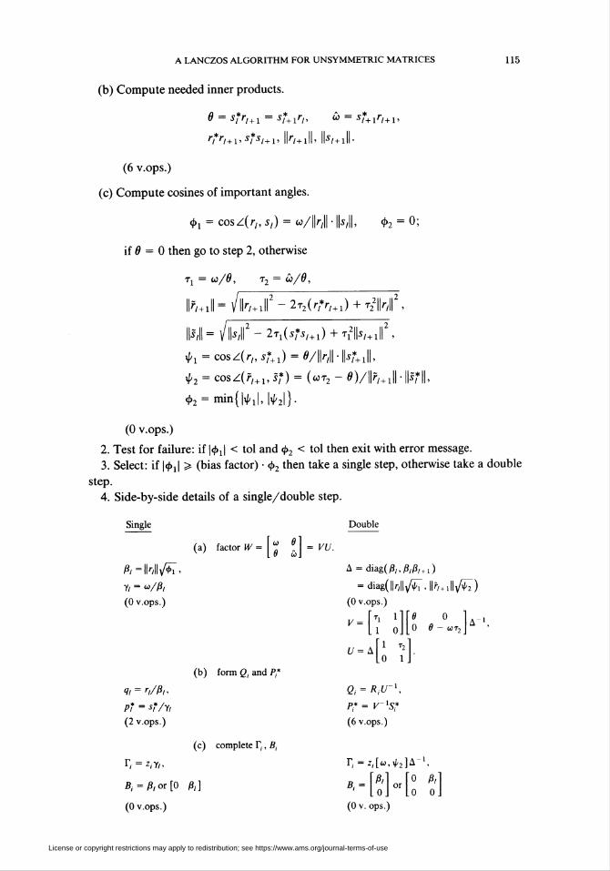
(b) Compute needed inner products.

9 = sfr,+i = sf+1r„ w = sf+1rl+1,

* * Il II II IIri r/+i> st si+i> llr/+ill' ll5/+ill-

(6 v.ops.)

(c) Compute cosines of important angles.

4>x = cosz(r„ s¡) = u/\\r,\\ ■ \\s,\\, <j>2 = 0;

if 0 = 0 then go to step 2, otherwise

Tx = CO/0, T2 = CÔ/0,

ll'mll = \/|k/+tl|2 - 2T2(r,*r/+1) + T2\\r\t,

P/ll = v IWI2 - 2ti(í*í/+i) + Ti2lk+ill2.

tx = cosz(rl,st+x) = 0/\\rl\\sT+x\\,

t2 = cosZ(fl+x, If) = (cot2 - 0)/||r/+1|| • ||s*||,

<¡>2 = miníj^l, \y¡i2\).

(0 v.ops.)

2. Test for failure: if |(p,| < toi and §2 < toi then exit with error message.

3. Select: if \<f>x\ > (bias factor) • <j>2 then take a single step, otherwise take a double

step.

4. Side-by-side details of a single/double step.

Single

¿8/Hk/IIV^i"'

Y/ = «/ft(0 v.ops.)

<& = n/ßi,

Pi = «*/»

(2 v.ops.)

r¡ = Z(Y/>

B, = ß, or [0

(0 v.ops.)

Double

(a) factor W = f " ? 1 = Kt/.

(b) form Qi and />,*

(c) complete T¡, B¡

A-diag(ft,ftft+1)

-diagdy^T.II^,!!^")(0 v.ops.)

V = îlllÖ 00 0 - UT,

Lo i

a-*,tr\/>,* = V 's*

(6 v.ops.)

rf-í(fi,^2]A-1,

"0 ft0 o

B, ft0

(0 v. ops.)


116 BERESFORD N. PARLETT, DEREK R. TAYLOR AND ZHISHUN A.LIU

Single

r,+ l =0+i/ft.

s/+i = i/+i/)7

(2 v.ops.)

a, = 1/t,

(0 v.ops.)

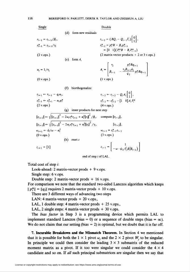
(d) form new residuals

Double

r,+2 = iBQ,-Q,-ir,)[°1

= [0 l](P*B - B,P*_X)

(2 matrix-vector products + 2 or 3 v.ops.)

(e) form/I,

A, -

PÎH+iTift+i^i

P*B1i+\

(f) biorthogonalize

ri+\ - ?/«/.

(1 v.ops.)

'1+2 '1+2 QA, i •«//>* [1 0] A,P,*

(2 v.ops.) (4 v.ops.)

(g) inner products for next step

Ik+ill *- Vll'V+tll2 - 2atr*rt+i + «¿hi /ft. compute ||r/+2||

*;+il «- Vll^+ill2 - 2ais*si+i + «?N|2/Y„

w/+i *~ "A0 — a/

(0 v.ops.)

h + x = [1]

(h) reset z

(3 v.ops.)

1

*,+1"[-«-M^/+i)

end of step i of LAL.

Total cost of step i:

Look-ahead: 2 matrix-vector prods + 9 v.ops.

Single step: 6 v.ops.

Double step: 2 matrix-vector prods + 16 v.ops.

For comparison we note that the standard two-sided Lanczos algorithm which keeps

ll/,*ll = 119/11 requires 2 matrix-vector prods + 10 v.ops.

There are 3 different ways of advancing two steps

LAN: 4 matrix-vector prods + 20 v.ops.,

LAL, 1 double step: 4 matrix-vector prods + 25 v.ops.,

LAL, 2 single steps: 4 matrix-vector prods + 30 v.ops.

The bias factor in Step 3 is a programming device which permits LAL to

implement standard Lanczos (bias = 0) or a sequence of double steps (bias = oo).

We do not claim that our setting (bias = 2) is optimal, but we doubt that it is far off.

7. Incurable Breakdown and the Mismatch Theorem. In Section 4 we mentioned

that it is possible for both the 1 X 1 pivot coy and the 2 X 2 pivot Wj to be singular.

In principle we could then consider the leading 3x3 submatrix of the reduced

moment matrix as a pivot. If it too were singular we could consider the 4x4

candidate and so on. If all such principal submatrices are singular then we say that



the breakdown at step y is incurable. In his thesis [11] Taylor proves the following

surprising consequence (Theorem 4.2) of this ultimate disaster.

Mismatch Theorem (Taylor). Let B have distinct eigenvalues and let Jj be the

block tridiagonal matrix produced by the Look-ahead Lanczos algorithm at step j. If

incurable breakdown occurs at step j + 1 then each eigenvalue of Jj is an eigenvalue of

B.

We add that neither span(P-) nor span(çV) is invariant under JS. The reason for

the name of the theorem becomes clear in the proof. Each starting vector must

contain components of eigenvectors that are not matched in the other starting

vector.

8. How to Monitor the Linear Independence of the Lanczos Vectors. In practice we

have found it convenient to normalize each Lanczos vector to have unit length,

II All = 119,-11 = 1- Consequently,

Pj*Qj =:% = diag(^,... Jj), *, > 0,

instead of the identity matrix. The formulas in both LAL and LAN must be changed

accordingly. Moreover, the "Ritz" values 0 at step j come from the generalized

eigenvalue problem

det(jj - 0%) = 0.

One incentive for making this change is that our technique for updating "Ritz"

values at each step (using the Hyman-Laguerre method [6]) extends without change

to the generalized eigenproblem.

Another advantage is that the elements of ^ indicate the quality of the Lanczos

bases {Pi,...,Pj), {qx,...,qj}. The standard measure of the linear independence of

the columns of a matrix is its condition number for inversion. Recall that

Pj-.= (px,...,pj) and

where Pj+ is the pseudo inverse of Pj. The normalization ||/>(.|| = 1, / = l,...,y,

ensures that

||p/:= ||P/Pj<||matrbcofl's||=y.

Similarly \\Qj\\2 <y. In exact arithmetic PfQj = Q*Pj ■ % = symmetric, and ¥, is

invertible. By checking the four Moore-Penrose conditions it can be verified that

(¿?)+-e,V, Q¡-*rx*r.So

For the regular Lanczos algorithm ||^._1|| = l/min1<i<y i|/,, and, in this case,

cond(P,) < ||Pj • ||e,-||/ min >,. < j/ min J,.



In practice, both ||P.|| and \\Qj\\ grow much more slowly than does jj. Eveny'1/4 is an

overestimate in the cases we have tried. However, for Lanczos runs limited to 200

steps the factory is not serious. With biorthogonalization maintained l/min1<;i< <//,

is a very good—and cheap—measure of the quality of the Lanczos bases.

However, without explicit biorthogonalization of the p¡ and qk the relation

Pj*Qj = ^fj fails completely as soon as an eigenvalue of the pair (Jj,^j) stabilizes

and after that point linear independence is lost for all practical purposes. There is no

point in monitoring the <//, after this point.

9. Numerical Examples. We give a few examples which contrast the performance

of the standard two-sided Lanczos algorithm and our Look-ahead variant. They

illustrate the stabilizing effect of the new variant.

All our computations were done on one of the VAX 11/780's of the Computer

Systems Research Group at the University of California, Berkeley.

The Look-ahead algorithm reduces to the regular algorithm when the bias

factor = 0. We kept the bias = 2 for all our examples.

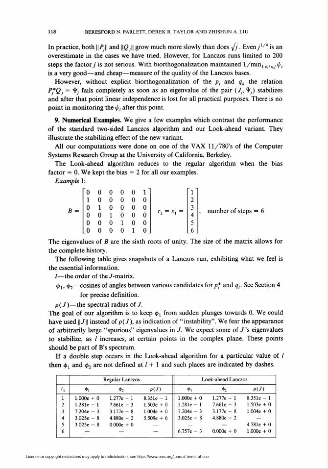
Example I:

B

001000

000100

000010

000001

number of steps = 6

The eigenvalues of B are the sixth roots of unity. The size of the matrix allows for

the complete history.

The following table gives snapshots of a Lanczos run, exhibiting what we feel is

the essential information.

/—the order of the /-matrix.

"Ei. 02—cosines of angles between various candidates for/»,* and q,. See Section 4

for precise definition.

piJ)—the spectral radius oiJ.

The goal of our algorithm is to keep <f>x from sudden plunges towards 0. We could

have used \\J\\ instead of piJ), as indication of "instability". We fear the appearance

of arbitrarily large "spurious" eigenvalues in J. We expect some of J's eigenvalues

to stabilize, as / increases, at certain points in the complex plane. These points

should be part of B's spectrum.

If a double step occurs in the Look-ahead algorithm for a particular value of /

then </>! and <f>2 are not defined at / + 1 and such places are indicated by dashes.

Regular Lanczos Look-ahead Lanczos

*i *> P(J) *1 h p(V)

l.OOOe + 0

1.281e - 1

7.204e - 3

3.025e - 8

3.025e - 8

1.277e - 1

7.661e - 3

3.177e - 8

4.880e - 2

0.000e + 0

8.351e - 1

1.503e + 0

1.004e + 0

5.509e + 6

l.OOOe + 0

1.281e - 1

7.204e - 3

3.025e - 8

6.757e - 3

1.277e - 17.661e - 3

3.177e - 8

4.880e - 2

0.000e + 0

8.351e - 1

1.503e + 01.004e + 0

4.781e + 0

l.OOOe + 0



Comment: Step 1-3 of both Regular and Look-ahead Lanczos are identical. At

step 4, Regular Lanczos normalizes s4 and r4 by factors of 10 "3, producing elements

in / of size 106. Step 5 Regular Lanczos is then aborted because the vectors are now

orthogonal to working precision.

The Look-ahead algorithm avoids the large element growth in /, by doing a

double step. The resulting /-matrix had eigenvalues identical to B to working

accuracy.

Example II: B is 12 X 12 block upper triangular with diagonal blocks shown

below. The other upper triangular elements Z»,7 were randomly distributed in [ - 5,5].

*i-

B6 =

B2 =95 2-2 95

25 -5050 25

rx = sx = [l,...,l]*.

Number of steps taken = 24.

2 -9595 2

, B3=[99], 2?4 = *s = [98],

, B7=[10-2], Bt50 -5050 50

Attributes. B is 12 X 12 and fairly far from normal. In particular, the five

eigenvalues near 97 form an ill-defined cluster because the off-diagonal elements in

the Schur form are all approximately the same magnitude as the separation between

Behavior of "Ritz" values approaching well separated eigenvalues

-30 .0 0.0 30.0 60.0 90.0 120.0

Figure 1

LAL with/without full rebiorthogonalization

A 7 well-isolated eigenvalues of B

D cluster of the remaining 5



these five eigenvalues. Only half the figures in the double eigenvalue 98 will be

significant and the other three eigenvalues are just a little better defined.

Results. 1. When full biorthogonalization was forced, the results from LAN and

LAL were essentially the same. The process halted at step 12 with the isolated

eigenvalues correct to at least 6 of the 7 decimals carried. The cluster was given as

95.001 ± 1.99921, 97.960 and 98.046, 98.991.Most of the ypi(= p*q¡) exceeded 0.1 (whereas i//, = 1 for symmetric matrices) but at

steps 9 and 10, i9 = 0.014 (for LAL), ̂ = 0.007 (for LAN).

2. When LAN and LAL were run with no biorthogonalization, they each lost

biorthogonality by step 10 but neither algorithm came close to breakdown. The

eigenvalue approximations were indistinguishable. By step 10 the 7 isolated eigenval-

ues were good to 6 decimals, in the neighborhood of the cluster of 5 each algorithm

produced 99.11 ± 3.26/ and 96.72. At step 12 the cluster of 5 is

95.14 ± 2.292/, 98.85 ± 0.604/, 91.75 according to LAL

but

94.96 ± 2.325/, 98.87 ± 0.577/, 45.6!! according to LAN.

However the residual error bounds do show that 45.6 is indeed spurious.

Neither algorithm halts at step 12, but step 24 exhibits a peculiar feature that we

cannot explain. Each algorithm has 12 Ritz values which are satisfactory approxima-

tions to the eigenvalues of B. Whereas the 12 extra Ritz values in LAN are very close

Behavior of "Ritz" values in the neighborhood of an ill defined cluster

4 .0

3.0

2 .0

1 .0

0 .0

1.0

10

12A

10--8 12012 1 2 A

-J_1_I_l_ ' ■ '

94.0 95.0 96.0 97.0 98.0 99.0 100.0

Figure 2

LAL with full rebiorthogonalization

A the 3 simple eigenvalues of B in the cluster

O the double eigenvalue 98.0



copies of the true eigenvalues, some extra Ritz values in LAL appear to be almost

random.

Figures 1 through 3 give some indication on how our LAL performs with or

without full rebiorthogonalization. The numerals show the first step at which the

Ritz value arrived at the indicated position. The dotted lines are an aid to

imagination but have no claim to be trajectories. An isolated a shows that the Ritz

value never wandered far from its first appearance. For well-isolated eigenvalues,

there was no essential difference with or without explicit rebiorthogonalization as

depicted in Figure 1.

Example III: Attributes. B is 15 X 15 upper triangular matrix with evenly-spaced

real eigenvalues ( - 65, - 55,..., - 5,0,5,..., 65). The superdiagonal elements were

randomly chosen numbers in the range ( -10,10). The diagonal elements were

[10/-75, y = l,...,7,

bjj- 0, y = 8,

\10y-85, y = 9,...,15.

'•! = *! = [1,1,...,1]*.

So this is an easy case from the point of view of the spectrum but it is, at the same

time, far from normal. The Lanczos vectors/», and q¡ are not close at all.

Behavior of "Ritz" values in the neighborhood of an ill defined cluster

4 .0

3 .0

2 .0

1 .0

0 .0

1 .0

12.

24

10--8

2 4' \

O 14

10

1.8 12,

2 4^-1!

J_,_

94 .0 95 .0 96.0 97 . 0 98 .0 99 .0 100 . 0

Figure 3

LAL without full rebiorthogonalization

a the 3 simple eigenvalues of B in the cluster

0 the double eigenvalue 98.0



Results. Excellent. No instability in LAN and consequently LAL used single steps

throughout and produced the same results. After 15 steps all eigenvalues were good

to 6 decimals (out of 7 carried) except for 0 which was represented by 3.4 X 10_5.

However, our stopping criterion was too strict to cause the algorithm to stop (the

off-diagonal elements only dropped by a factor of 1000). After step 15, the two

algorithms began to differ but by step 30 both had essentially obtained duplicates of

the 15 eigenvalues.

With any form of biorthogonalization both algorithms terminated at step 15 with

eigenvalues correct to at least 6 figures. The zero eigenvalue was given as 6 x 10 ~8

+ 1.1 x 10-10/.

Example IV: Attributes. B is 100 X 100, diagonal, with distinct eigenvalues.

B = diag(l, 2,..., 20,41,62,..., 440,481,522,..., 1260,1331,1382,...,

2480,2561,2642,... ,4019,4100).

The interest here was to start with px and qx different and random. In fact

ix=p*xqx = 0.06.

7=o iy=10-4 n=10-3

[io-3i]

30 -

20

10 -

1 --f *-

(22)Steps for

convergence

(20)

(17)

(13)

(9)

■4 f-0 0

Figure 4

Spectrum of ( F, M ), n = 94



Results. Disappointing at first. After 19 steps the largest eigenvalue was good to 4

figures (4099.8) but no others had converged recognizably. However, the gap ratio

(Aioo ~ A99)/(^ioo _ Ai)> which governs the convergence rate, is only 0.02 and

consequently even with px = qx convergence will not be much faster. See [12,

Chapter 12] for a fuller explanation. One interesting feature, not yet explained, is an

unbalanced loss of biorthogonality. For example,p*qX3 ~ e,p\*3q3 ~ 105e. At step 13

\px3 dropped to 5 X 10"4 and most \¡/¡ were less than 10"2.

We conclude that it is a mistake to begin with nearly orthogonal px and qx unless

they are known to be approximate eigenvectors of the same eigenvalue.

Example V: Attributes. The Max Planck Institute in Munich has supplied us with

programs to generate matrices of the form B = F~lM arising in the study of plasma

instability; of course, F is not inverted explicitly. There is a parameter rj (resistivity)

which can be varied. When tj = 0 all the eigenvalues are pure imaginary. Only the

largest few eigenvalues are of interest.

We have tried our codes on matrices of order n = 34, 94 and 598.

Results. Excellent. With a random starting vector (px = qx) the largest 8 eigenval-

ues converged to working accuracy in fewer than 30 steps. This phenomenon is

independent of n, the size of the matrix. The dominant eigenvalue usually converged

after 10 steps.

Figure 4 shows how the (reciprocals of) the eigenvalues leave the imaginary axis as

tí increases from 0.

10. Conclusion. The Look-ahead algorithm (LAL) is more complicated than the

standard two-sided Lanczos process (LAN). We have so far found only one case

(Example I) in which LAN fails while LAL succeeds. Often they both perform very

satisfactorily. Each can be used with rebiorthogonalization of the left and right

Lanczos vectors against each other. This safeguard increases the cost but makes the

results very close to those produced by exact arithmetic. For short runs (y < 30) on

vector computers this extra cost of explicitly forcing the Lanczos vectors to be

biorthogonal may be a small fraction of the cost of the other parts of the algorithm.

The principal reason for consenting to use two sequences of vectors (Py and Qf)

instead of one (as in Arnoldi's method, see [9]) is the expectation of convergence of

the dominant eigenvalues after a small number of steps. When both the column and

row subspaces contain, respectively, \/e approximations to the eigenvectors of X then

one of the Ritz values will be an e-approximation to X. This cannot happen with

one-sided approximations unless the matrix is normal.

LAL is an effective tool for extracting a few eigenvalues of large nonnormal

matrices. Whether it is better than its rivals remains to be seen. At such a time it will

be appropriate to discuss computable error estimates, efficient ways to monitor

convergence of the eigenvalues of /., and other practical details.

Center for Pure and Applied Mathematics

University of California

Berkeley, California 94720

1. C. Davis & W. Kahan, "The rotation of eigenvectors by a perturbation—III," SIAM J. Numer.

Anal., v. 7,1970, pp. 1-46.

2. W. Gragg, Notes from a "Kentucky Workshop" on the moment problem and indefinite metrics.

3. A. S. Householder, The Theory of Matrices in Numerical Analysis, Blaisdell, New York, 1964.



4. W. Kahan, B. N. Parlett & E. Jiang, "Residual bounds on approximate eigensystems of

nonnormal matrices," SIAM J. Numer. Anal., v. 19,1982, pp. 470-484.

5. C. Lanczos, "An iteration method for the solution of the eigenvalue problem of linear differential

and integral operators," J. Res. Nat. Bur. Standards, v. 45,1950, pp. 255-282. See pp. 266-270.

6. B. N. Parlett, "Laguerre's method applied to the matrix eigenvalue problem," Math. Comp., v. 18,

1964, pp. 464-487.7. B. N. Parlett, The Symmetric Eigenvalue Problem, Prentice-Hall, Englewood Cliffs, N. J., 1980.

8. B. N. Parlett & J. R. Bunch, "Direct methods for solving symmetric indefinite systems of linear

equations," SIAMJ. Numer. Anal., v. 8,1971, pp. 639-655.

9. Y. Saad, "Variations on Arnoldi's method for computing eigenelements of large unsymmetric

matrices," Linear Algebra Appl., v. 34,1980, pp. 269-295.

10. Y. Saad, "The Lanczos biorthogonalization algorithm and other oblique projection methods for

solving large unsymmetric eigenproblems," SIAMJ. Numer. Anal., v. 19,1982, pp. 484-500.

11. D. R. Taylor, Analysis of the Look Ahead Lanczos Algorithm, Ph.D. thesis, University of

California, Berkeley, 1982.

12. J. H. Wilkinson, 77i<? Algebraic Eigenvalue Problem, Oxford Univ. Press, Oxford, 1965.


A Look-Ahead Lanczos Algorithm - AMS

Documents

Transcript of A Look-Ahead Lanczos Algorithm - AMS